Multi-TRxPs for IndustrialAutomation with 5G URLLCRequirements

Farah Salah

School of Electrical Engineering

Thesis submitted for examination for the degree of Master ofScience in Technology.

Espoo 26.11.2018

Supervisor

Prof. Riku Jäntti

Advisor

Lauri Kuru

Copyright c⃝ 2018 Farah Salah

Aalto University, P.O. BOX 11000, 00076 AALTOwww.aalto.fi

Abstract of the master’s thesis

Author Farah Salah

Title Multi-TRxPs for Industrial Automation with 5G URLLC Requirements

Degree programme Electrical Engineering

Major Communications Engineering Code of major ELEC3029

Supervisor Prof. Riku Jäntti

Advisor Lauri Kuru

Date 26.11.2018 Number of pages 62 + 10 Language English

AbstractThe Fifth Generation (5G) Ultra Reliable Low Latency Communication (URLLC)is envisioned to be one of the most promising drivers for many of the emerginguse cases, including industrial automation. In this study, a factory scenario withmobile robots connected via a 5G network with two indoor cells is analyzed. Theaim of this study is to analyze how URLLC requirements can be met with the aid ofmulti-Transmission Reception Points (TRxPs), for a scenario which is interferencelimited. By means of simulations, it is shown that availability and reliability can besignificantly improved by using multi-TRxPs, especially when the network becomesmore loaded. In fact, optimized usage of multi-TRxPs can allow the factory tosupport a higher capacity while still meeting URLLC requirements. The resultsindicate that the choice of the number of TRxPs which simultaneously transmit toa UE, and the locations of the TRxPs around the factory, is of high importance. Apoor choice could worsen interference and lower reliability. The general conclusionis that it is best to deploy many TRxPs, but have the UE receive data from onlyone or maximum two at a time. Additionally, the TRxPs should be distributedenough in the factory to be able to properly improve the received signal, but farenough from the TRxPs of the other cell to limit the additional interference caused.

Keywords Industrial Automation, URLLC, Multi-TRxP, Spatial Diversity, 5G, NR

iv

Preface

I would like to offer my most sincere gratitude to my professor Riku Jäntti for hisvaluable feedback and guidance. I would also like to thank my advisor Lauri Kuruwho has been an unfaltering source of support throughout this experience. Manythanks to all my colleagues at Nokia who have inspired me, and readily offered theirhelp whenever it was needed. I have been provided with an excellent environmentin which I could grow, learn, and conduct my research, and for this I will remaineternally grateful. Additionally I would like to extend my deepest appreciation to allthe great teachers who have taught me both in Jordan and in Finland, for performingthe world’s most important job. Last but not least, I would like to thank my family,whom I owe all of my life’s successes to, and my friends everywhere, whom I am verylucky to have.

Otaniemi, 26.11.2018

Farah Salah

v

Contents

Abstract iii

Preface iv

Contents v

Symbols and abbreviations viii

1 Introduction 1

1.1 Motivation . . . . . . . . . . . . . . . . . . . . . . . . . . . . . . . . . 1

1.2 Objectives and Research Questions . . . . . . . . . . . . . . . . . . . 3

1.3 Thesis Structure . . . . . . . . . . . . . . . . . . . . . . . . . . . . . . 4

2 Background 5

2.1 Reliability Definitions in General . . . . . . . . . . . . . . . . . . . . 5

2.2 Reliability Definitions within Communication Systems . . . . . . . . . 6

2.3 Reliability, Latency, and Capacity Trade-offs . . . . . . . . . . . . . . 7

2.4 5G Architecture and Assumptions . . . . . . . . . . . . . . . . . . . . 8

2.5 Dual Connected Handover . . . . . . . . . . . . . . . . . . . . . . . . 9

2.6 MMIB-based L2S Interface and Link Adaptation . . . . . . . . . . . . 12

3 Factory Scenario 15

3.1 Use Case Selection . . . . . . . . . . . . . . . . . . . . . . . . . . . . 15

3.2 Characteristics . . . . . . . . . . . . . . . . . . . . . . . . . . . . . . 15

3.3 Requirements . . . . . . . . . . . . . . . . . . . . . . . . . . . . . . . 16

3.4 Propagation Environment . . . . . . . . . . . . . . . . . . . . . . . . 18

vi

4 Reliability Enhancement with Multi-TRxP Solution 20

4.1 Deployment and Setup . . . . . . . . . . . . . . . . . . . . . . . . . . 22

4.2 Multi-point Transmission/ Reception and Coordination Methods . . . 24

4.3 Simple Analytic Proof . . . . . . . . . . . . . . . . . . . . . . . . . . 27

5 Simulation Work 30

5.1 Simulation Assumptions and Main Parameters . . . . . . . . . . . . . 30

5.2 Defining URLLC KPIs . . . . . . . . . . . . . . . . . . . . . . . . . . 34

5.3 Development Methodology and Modifications to the Simulation Tool 38

6 Results and Analysis 40

6.1 Initial Observations . . . . . . . . . . . . . . . . . . . . . . . . . . . . 40

6.2 TRxP Cluster Size Sweep . . . . . . . . . . . . . . . . . . . . . . . . 41

6.2.1 With 50 factory UEs . . . . . . . . . . . . . . . . . . . . . . . 41

6.2.2 With 70 factory UEs . . . . . . . . . . . . . . . . . . . . . . . 43

6.2.3 With Variable Capacity . . . . . . . . . . . . . . . . . . . . . 45

6.3 Number of Existing TRxPs per cell Sweep . . . . . . . . . . . . . . . 45

6.3.1 With 50 factory UEs . . . . . . . . . . . . . . . . . . . . . . . 46

6.3.2 With 70 factory UEs . . . . . . . . . . . . . . . . . . . . . . . 46

6.4 TRxP Ring Radius Sweep . . . . . . . . . . . . . . . . . . . . . . . . 49

6.4.1 With 50 factory UEs . . . . . . . . . . . . . . . . . . . . . . . 49

6.4.2 With 70 factory UEs . . . . . . . . . . . . . . . . . . . . . . . 49

6.5 System Statistics and Confidence Intervals . . . . . . . . . . . . . . . 51

7 Conclusion 55

7.1 Summary . . . . . . . . . . . . . . . . . . . . . . . . . . . . . . . . . 55

7.2 Evaluation and Limitations . . . . . . . . . . . . . . . . . . . . . . . 56

vii

7.3 Future Work . . . . . . . . . . . . . . . . . . . . . . . . . . . . . . . . 58

References 59

viii

Symbols and abbreviations

Symbols

Tc Coherence Timefm Maximum Doppler Spreadfc Central Frequencyv Velocityc Speed of Light in a Vacuumd Distanced0 Reference Distancen Path Loss ExponentPs Desired Signal PowerPi Interference PowerN Noise PowerD DowntimeU UptimeT Total Time IntervalNU Number of Uptime EventsDU Number of Downtime Events

Abbreviations

3GPP Third Generation Partnership Project4G Fourth Generation Mobile Network5G Fifth Generation Mobile NetworkAS Active setAVG Automated Guided VehiclesBLEP Block Error ProbabilityBLER Block Error RateCBR Constant Bit RateCDF Cumulative Distribution FunctionC-JT Coherent Joint TransmissionCL Confidence LimitC-MTC Mission-Critical MTCCN Core NetworkC-plane Control PlaneCQI Channel Quality IndicatorC-RAN Cloud-RANCSI Channel State InformationCSI- RS Channel State Information Reference SignalCU Central UnitCW Code Word

ix

D2D Device to Device CommunicationDCHO Dual Connected HandoverDD Data DuplicationDL DownlinkDM-RS Demodulation Reference SignalDPS Dynamic Point SelectionDU Distributed UnitE2E End-to-EndFLS Fast Link SwitchinggNB Next Generation NodeBHO HandoverJT Joint TransmissionKPI Key Performance IndicatorL2S Link to SystemL1 Layer 1L3 Layer 3LA Link AdaptationLOS Line-of-SightLSF Large-Scale FadingLTE Long Term EvolutionLUT Look-up TableMAC Media Access ControlMCBF Mean Count Between FailuresMCS Modulation and Coding SchemeMI Mutual InformationMIMO Massive Input Massive OutputMIT Mobility Interruption TimeMMIB Mean Mutual Information per BitM-MTC Massive MTCMTBF Mean Time Between FailuresMTC Machine Type CommunicationMTTR Mean Time to RecoverNC-JT Non-Coherent Joint TransmissionNR New RadioNR-PDSCH New Radio-Physical Downlink Shared ChannelOBS Obstructed Line-of-SightPCI Physical Layer Cell IdentityPDCP Packet Data Convergence ProtocolPER Packet Error ProbabilityPHY Physical LayerPL Path LossPRB Physical Resource BlockQoS Quality of ServiceRAN Radio Access NetworkRBIR Received Bit Information Rate

x

RLC Radio Link ControlRLF Radio Link FailureRRC Radio Resource ControlRRM Radio Resource ManagementRS Reference SignalRSRP Reference Signal Received PowerRx Receiver AntennaSDAP Service Data Adaptation ProtocolSDU Service Data UnitSE Spectral EfficiencySI Symbol InformationSINR Signal to Interference and Noise RatioSNR Signal to Noise RatioSRB Signaling Radio BearerSRS Sounding Reference SignalTRxP Transmission Reception PointTTI Transmission Time IntervalTTT Time to TriggerTx Transmitter antennaUE User EquipmentUL UplinkUPF User Plane FunctionU-plane User PlaneURLLC Ultra-Reliable Low-Latency Communications

1 Introduction

The promises of what the Fifth Generation Mobile Network (5G) will enable hassparked innovation and created a vision of a new 5G-era with seemingly endlesspossibilities. It has caused the emergence of new paradigms of thought, new ways toconduct business, new technological solutions, services and products, and is expectedto transform the world as we know it. With the advent of some of those newtechnologies and use cases which deviate from the traditional human-centric, delaytolerant applications, the need for Ultra-Reliable Low-Latency Communications(URLLC) in the 5G wireless network has become incontrovertible. Within URLLC,mobility is a major concern as it increases systems’ vulnerability to interference,shadowing, and other hindrances which lower the signal quality and cause unreliablecommunication. This thesis studies how stringent URLLC requirements can bemet even when users are mobile, by using multiple Transmission Reception Points(multi-TRxP). In this chapter, the motivation towards adopting 5G networks withURLLC for industrial automation scenarios is given, followed by the objectives andresearch questions of this thesis work, and finally a brief outline of the thesis.

1.1 Motivation

One of the major differentiators of 5G from any of the previous generations ofmobile wireless systems is that it is natively addressing the needs of Machine-Type Communications (MTC). The Third Generation Partnership Project (3GPP)classifies MTC into two categories; Massive MTC (M-MTC), and Mission-CriticalMTC (C-MTC) [1]. M-MTC consists of a large number of low-cost, low-energydevices such as sensors and actuators, which communicate with low data volumes,and require networks with high coverage and energy efficiency. On the other hand,C-MTC involves scenarios that require ultra reliability, with very low latency and veryhigh availability. URLLC is one of the most promising innovation-driving featuresof 5G, as it enables such C-MTC applications as industrial automation, smart grid,remote surgery, self-driving cars and Vehicle to Vehicle (V2V) as well as Vehicleto Infrastructure (V2I) communication. A summary of MTC use cases is shown inFigure 1.

In this work, industrial automation is taken as an example target use case forpossibly very strict URLLC requirements. Automation within factories is continuouslyincreasing, as it increases productivity and operational efficiency, and reduces costsand manufacturing errors. Automation helps industries to efficiently monitor, manage,and control their processes. In fact, URLLC has been said to be "one of the enablingtechnologies in the fourth industrial revolution" [2].

Traditionally, wired networks have been used because the existing wireless tech-nologies were not capable of satisfying the required latency and reliability requirements.

2

Figure 1: Machine Type Communication Use Cases for 5G.[1]

However, wired communication also comes with a wide range of problems, includingwear and tear of the wires reducing long-term reliability, high costs of manufacturing,installing, and maintaining, as well as inherent inflexibility of deployment, whencompared to the wireless alternative. The advantages of wireless communication forindustrial automation applications are numerous. To begin with, production lineconfiguration is flexible and modular, there can be a rapid realization of differentproduction environments, and the communication between devices is flexible. Inaddition, mobility is easy since slip rings, cable carriers, etc., can be avoided formachines, robots or sensors. Installation and maintenance costs are also lower, due tothe absence of cable damages from moving machine parts, no protection and housingneeds, faster installation, and no interruptions by the personnel.

Therefore, wireless communication for industrial automation has been on a steeprise, and is expected to continue growing extensively. In fact, a research reportby Persistence Market Research predicts that the revenue from global markets forindustrial wireless sensor networks will reach approximately US$ 7,000 Million bythe end of 2026, due to increased demand from the growing implementation ofautomation technologies [3].

However, there are many challenges that arise from using wireless communication,due to the nature of electromagnetic wave propagation. Reflection, scattering,and diffraction which electromagnetic waves experience result in constructive ordestructive interference of different signal copies arriving at the receiver, causing ahigh fluctuation of the quality of wireless transmission channels. These problemsbecome even more prominent in industrial propagation environments which tendto have many metallic surfaces and moving objects. This is one of the reasonswhy the currently available wireless access technologies limit the possibility of usingwireless communication for automatic industries with high reliability constraints. Forinstance, connecting factory User Equipment (UE) via WiFi or any other technologywhich operates in the unlicensed band leads to many restrictions due to concerns

3

such as security, privacy, and potentially very high interference. The current fourth-generation (4G) wireless cellular network, also known as Long Term Evolution (LTE),is also not suitable, as it is unable to satisfy strict latency or reliability requirements.Simulation results in [4] show that LTE can indeed support factory scenarios but onlywhen relaxed reliability and delay requirements are targeted, however with stringentrequirements a new 5G radio-interface is needed. The nominal latency of LTE isaround 50 ms, and might even reach several seconds [5]. LTE is also designed toserve mostly mobile broadband traffic, which does not have very high reliability. Infact its target Block Error Rate (BLER) is approximately 10-1 before re-transmission.Meanwhile, Table 1 shows that factory reliability requirements can lead to BLERtarget of 10-9 and latency of as low as 1ms. This table is a result of a survey whichgathered first-hand information from notable industry players [6]. Therefore, there isa vital need for factories of the future to be able to operate their devices over the5G network, and potentially acquire their own frequency bands, benefiting from thegeneral advantages of a licensed band, in addition to the improved reliability, latency,and flexibility of 5G. For this reason, this work focuses on how industrial automationscenarios using 5G networks can meet stringent URLLC requirements.

Table 1: Machine Type Communication Use Cases for 5G.[6]

E2ELatency

Reliability Data Size Com.RangeBetweenDevices

No. ofDevicesperFactoryHall

MachineMobility(Indoors)

Summarized Results1 to 50 ms 1 − 10−6 to

1 − 10−910 to 300bytes

2 to 100 m 10 to 1000 0 to 10 m/s

Application Scenario: Manufacturing Processes< 10 ms 1 - 10−9 < 50 bytes < 100 m < 1000 1 m/s

Application Scenario: Automated Guided Vehicles10 to 50 ms 1 − 10−6 to

1 − 10−9< 300 bytes 2 m < 1000 < 10 m/s

1.2 Objectives and Research Questions

This work studies how stringent URLLC requirements can be met in industrialautomation scenarios by using multi-TRxPs, which provide spatial diversity gains.The work includes defining the most relevant and representative reliability Key

4

Performance Indicators (KPIs) for communication networks, quantifying those KPIs,and using them to study reliability by means of simulation. A Nokia internal systemlevel simulation tool is used, and support for the multi-TRxP solution is added to thecode. Factory automation with mobile robots as UEs is selected as a relevant use case,but results can be extended to a wide range of applications. Dual Connected Handover(DCHO) and Mean Mutual Information per Bit (MMIB)-based Link Adaptation(LA) are incorporated in the baseline, and the study focuses on how reliability canbe improved further, while also considering capacity issues.

The primary research question is therefore, "How can the Multi-TRxP so-lution be optimally utilized for reliability and availability enhancementin an industrial automation scenario with URLLC requirements?". Theperformance is analyzed under three main themes, namely, the effect of the numberof TRxPs in a UE cluster, the number of TRxPs existing per cell, and the placementof TRxPs around the factory, which are explained in more details in further sections.These themes are studied for factories with two different capacity conditions; alow-medium loaded factory with 50 UEs, and a slightly overloaded factory with 70UEs. This gives insight into the ability of the solution to address capacity concerns.

1.3 Thesis Structure

The thesis is organized as follows. The background given in Section 2 starts byproviding reliability definitions in the context of reliability engineering in general, andthen within communication systems specifically. This is followed by some backgroundon the trade-off between reliability and latency on one hand, and capacity on theother. Then, a brief description is given of some aspects of 5G architecture andassumptions that are most relevant for this work. The background section concludesby discussing the dual connected handover and MMIB-based link to system interfaceand link adaptation, which are to be used in the study. Then, Section 3 provides adescription of the factory automation scenario which is to be simulated and analyzed.A justification of the selected use case is given, in addition to the specific set ofcharacteristics, requirements, and propagation environment that the use case pertains.Next, Section 4 introduces the multi-TRxP solution which the thesis studies as apotential method for achieving URLLC requirements within the industrial automationscenario. Here, the possible options for network deployment and setup, as well asthe multi-point transmission methods are discussed, and the selected choices arejustified. A small analytic proof of how multi-TRxPs can actually improve reliabilityin a simplified scenario is also given. From here, the thesis transitions into Section5, which discusses the simulation work. It includes the assumptions and mainparameters, and the URLLC KPIs that will be used to analyze the simulation results.In addition, a brief description of the modifications that were done to the simulationtool is given. Finally, the results are presented and analyzed in Section 6, and thework is concluded in Section 7, which includes an evaluation of the limitations of thestudy and suggestions for future work.

5

2 Background

2.1 Reliability Definitions in General

Before attempting to analyze and improve reliability, it is vital that the respectivedefinitions of key terms are properly understood and distinguished. Three of themost commonly used terms in reliability engineering are reliability, availability, andmaintainability. Those terms are central elements of many application areas, frommanufacturing, transport, and process industries, to nuclear and space industries.Their general definitions are known, but they can have very different applicablemeanings depending on the application, which is why some ambiguity exists inmuch of the literature. For this reason, the general definitions of those terms withinreliability engineering are given in this section based on the glossary of the AmericanSociety for Quality (ASQ) [7], followed in the next section by their specific andapplied definitions within communication systems.

• Reliability: "The probability of a product performing its intended functionunder stated conditions without failure for a given period of time" [7]. Reliabilitythen denotes the probability of a failure occurring over a specified time interval.It gives an indication of how long correct operation continues. Within a certainapplication area, a precise definition of reliability would need to include acomprehensive description of what the environment is, what the time period is,and how failures are defined, which could prove to be quite challenging.

• Availability: "The ability of a product to be in a state to perform its desig-nated function under stated conditions at a given time" [7]. It represents theprobability that a system is operational at a given point in time. Availabilityconsists of both reliability and maintainability.

• Maintainability: "The probability that a given maintenance action for an itemunder given usage conditions can be performed within a stated time interval whenthe maintenance is performed under stated conditions using stated proceduresand resources." [7]. Maintainability indicates how the system can be restoredafter a failure.

Figure 2 shows the relationship between those terms. From the figure, twonew acronyms appear; MTBF and MTTR. Those are respectively the Mean TimeBetween Failures and Mean Time To Recover, and are commonly used to quantifyreliability and maintainability. MTBF excludes downtime, while MTTR representsthe mean downtime. Clearly, an unreliable system can have high availability if itfixes itself instantly.

The following is a numerical example. If a certain system has an availability of99,999% (commonly referred to as 5 nines), then its unavailability is 0,001%, or 5

6

Figure 2: Availability, Reliability and Maintainability.

minutes on average per year. If failures occur in the system four times a year onaverage, then reliability, quantified as the MTBF, would be three months.

2.2 Reliability Definitions within Communication Systems

In this section, network reliability, availability, and maintainability are defined withinthe context of communication systems. Precise and applicable definitions are neededin order to use them during this study and consequent simulation analysis.

• Communication Service Reliability: TR 22.804 [8] defines reliability ac-cording to its definition in IEC 61907 [9], which closely agrees with the abovegiven general definition of reliability. It states that reliability is "the abilityof the communication service to perform as required for a given time interval,under given conditions". Those given conditions would "include aspects thataffect reliability, such as: mode of operation, stress levels, and environmentalconditions" [9]. Appropriate measures of quantifying reliability, according toTR 22.804, include "mean time to failure, or the probability of no failure withina specified period of time" [8]. This definition focuses on the end-to-end experi-ence of functions consuming the network’s communication capabilities, insteadof the inner workings of the network. One or more re-transmissions of networklayer packets may take place in order to satisfy the reliability requirement.

• Communication Service Availability: TR 22.804 defines communicationservice availability as the "percentage value of the amount of time the end-to-endcommunication service is delivered according to an agreed Quality of Service(QoS), divided by the amount of time the system is expected to deliver theend-to-end service according to the specification in a specific area" [8]. Simplyput, it is the percentage of time during which a system operates correctly.The end point in the definition’s mention of "end-to-end" is assumed to be thecommunication service interface. Note that a communication service which doesnot meet the relevant QoS requirements is considered to be unavailable. Forexample, a system can be considered unavailable even if the expected messageis correctly delivered, but not within the required time. This specified timeinterval cannot be shorter than the sum of the end-to-end latency, the jitter, and

7

the survival time. The survival time is "the time that an application consuminga communication service may continue without an anticipated message." [8].

• Communication Service Maintainability: this can be quantified by suchindicators as the mean time to restoration, or the probability of restorationwithin a specified period of time [9].

2.3 Reliability, Latency, and Capacity Trade-offs

Redundancy methods have long been used in several application fields to enhancereliability. Within communication systems, redundant links that transmit the sameinformation over different paths can drastically enhance the probability of successfuldelivery, especially when the paths are in different locations, granting more spatialdiversity. Many propagation problems are location-specific, which means that themore TRxPs that are deployed and sending the same information to a UE, the morelikely that at least one of them does so successfully. However, this does not comewithout a cost. The main problem with any redundancy method is waste. If a certainnumber of connected TRxPs is enough to ensure the desired level of reliability to theUE, any additional connection is wasteful, and would better be utilized to transmitnew data. This creates capacity limitations for user traffic. Moreover, additionalTRxPs are also creating more interference to other cells, and the greater the load onthe cell, the more the interference it causes is. This limits capacity as well.

Capacity is an important aspect of this study due to its importance in industrialautomation. The available spectrum can be rather limited, especially for the privatenetworks which are envisioned for many of the URLLC scenarios, such as the factoryautomation scenario. Spectral scarcity is an even bigger concern for networksoperating in frequency ranges below 6 GHz. The following is an example to clarifythis, which is based on traffic assumptions taken from TR 22.804 [8]. Considera packaging machine with 50 sensors, message size of 40 Bytes, and 1 ms cycletime. This translates to 40 * 8 * 50 *1000 = 16 Mbits/s + overheads, which isapproximately 20 Mbits/s/machine at L1. Due to the strict reliability and latencyrequirements, Spectral Efficiency (SE) can be rather low. If 1bps/Hz is assumed,which can still be considered quite optimistic, this translates to approximately 20MHzper machine on average. In conclusion, even one machine is capable of approachingthe capacity limits of a single 20 MHz carrier. If the machine happens to be at celledge, the situation could be even worse.

Capacity can be quite limited due to interference concerns. Additional UEsand/or higher user traffic increases interference, and therefore is likely to be limitedin order to achieve a certain reliability target. In addition, increasing the numberof TRxPs connected to each UE also increases the interference to other cells. Thisis specific to the scenario’s own deployment and setup, which is properly detailedin Section 4.1. Capacity and Spectral Efficiency (SE) can be quite limited and a

8

trade-off between SE and reliability requirement is expected, subject to interferenceconditions. TR 22.804 specifies a number of use cases with varying requirements,and the selected use case for this work assumes a maximum limitation of 100 mobilerobots. Section 3.3 further discusses the use case requirements, and the associatedlimitations caused by the available technology.

In order to allow for more capacity, the number of TRxP connections cannot beindefinitely increased, and an optimal number of TRxP connections that sufficesfor a certain level of reliability target likely exists. In addition, capacity can beincreased by using proper link adaptation, which selects an appropriate Modulationand Coding Scheme (MCS), that is low enough to improve the Signal to Interferenceand Noise Ratio (SINR) to meet the reliability Block Error Probability (BLEP)target, without reserving too many excess resources for a single transmission. Thisis further discussed in section 2.6. If a fixed, low, MCS is used, it will cause plentyof unnecessary interference and the resulting capacity will not be realistic.

When evaluating capacity, the specific variables that affect it for the particularfactory scenario must be taken into account. Those variables include the applicationrequirements, such as the target reliability and delay, as well as the traffic. Thetraffic characteristics include the message length and interval, traffic density, anddistribution.

2.4 5G Architecture and Assumptions

The 5G New Radio (NR) interface provides for the growing needs for mobile con-nectivity. Two fundamental technological enablers include softwarization, such asvirtualisation of network functions, as well as software defined, programmable net-work functions and infrastructure resources. The Next Generation NodeB (gNB)functions are split between a Central Unit (CU) and a Distributed Unit (DU). TheCU controls the operation of DUs over front-haul (Fs) interface. The DU is a logicalnode which includes a subset of the gNB functions, depending on the functional splitoption. In 5G release 15, TS38.401 defines the CU and DU according to the chosenfunctional split as follows:

• CU: a logical node hosting the Radio Resource Control (RRC) protocol, ServiceData Adaptation Protocol (SDAP) and Packet Data Convergence Protocol(PDCP) of the gNBs. The CU terminates the F1 interface connected with theDU. [10]

• DU: a logical node hosting Radio Link Control (RLC), Media Access Control(MAC) and Physical (PHY) layers of the gNB, and its operation is partlycontrolled by the CU. The DU terminates the F1 interface connected with theCU. A gNB may consist of a gNB-CU and one or more gNB-DU(s). One DU

9

can support one or multiple cells, but one cell can be supported by only oneDU. A gNB-CU and a gNB-DU is connected via F1 interface. [10]

Figure 3 shows one possible architecture option for gNBs. The figure shows theUser Plane Function (UPF) as part of the 5G Core Nework (CN), with two gNBsconnected, each with a CU and DU, and each DU with multiple TRxPS. The UserPlane interfaces shown in the figure are the New Generation User Plane interface(NG-U), which is between NG-RAN and 5G CN, the F1 User Plane interface (F1-U),which is between gNB-CU and gNB-DU, and the Xn User Plane interface (Xn-U),which exists between gNBs. Because the TRxPs within one cell in this option arecontrolled by the same DU, they share common scheduling and Layer 1 (L1) signals.This option is sufficient for the purpose of this work, and therefore the entire systemarchitecture is omitted from the scope of this thesis.

Figure 3: 5G NR Protocol Stacks with Two Cells and Multiple TRxPs.

2.5 Dual Connected Handover

TR 38.913 defines Mobility Interruption Time (MIT) as "the shortest time durationsupported by the system during which a user terminal cannot exchange user planepackets with any base station during transitions" [11]. The technical report alsostates that the target for mobility interruption time should be 0 ms for NR. CurrentLTE systems’ intra-frequency handovers suffer from failure risks which can causesevere user plane interruptions. Interruptions can be caused by both successful andfailed handovers. Field measurements in [12] show that 4G handovers each have amedian interruption time of 50 ms, and some handovers can lead to interruption

10

times of 80 to 100 ms. This makes mobility a big concern for URLLC. UnderURLLC requirements, failures cannot be tolerated, and successful handovers need tobe completed without introducing any interruptions. From the reliability’s point ofview purely, the legacy HO may not be completely out of question, but this essentiallydepends on the network loading and interference. However, from a latency pointof view, the legacy handover is not capable of satisfying the strictest requirements.Some improvements have been specified in LTE to reduce the delay down to theorder of approximately 10 ms, but 1 ms cannot be achieved with only one RX/TXchain. For example, Rel.14 make-before-break and synchronous Random AccessChannel (RACH)-less HO have been claimed to improve interruption time down toapproximately 5 ms in good conditions [13][14]. RACH-less HO allows to save theRACH procedure, whereas make-before-break keeps the UE connected to the sourcecell until it fully accesses the target cell. It is important to further note that this isfor successful handovers, and failed ones lead to significantly longer interruptions.For example, Radio Link Failure (RLF) timers are in the order of several hundredsof milliseconds.

Consequently, URLLC requirements raise the need for a handover that causes0 ms interruption. The interruption time will always be non-zero if the UE canonly connect to one cell at a time, since before connecting to a target cell it willhave to detach from the source cell. Therefore, 3GPP has started discussions ofwhat shall be referred to as a Dual Connected Handover (DCHO) hereinafter. WithDCHO, the UE will be able to connect simultaneously to both the source as wellas the target cell during a handover, leading to zero interruption time. For thistype of dual connectivity, both U-plane and C-plane will be anchored in the mastergNB (MgNB), and data bearers are split in the master’s Packet Data ConvergenceProtocol (PDCP) layer, so that there is an Xn interface after the PDCP layers of boththe MgNB and the Secondary gNB (SgNB). Note that instead of dual connectivity,multi connectivity could be considered. However, the gains of having more than 2connected cells for the handover are yet to be shown, and there is a possibility ofthe additional interference from those additional links even reducing reliability. Forthis reason, combined with the fact that legacy handovers are incapable of meetingURLLC’s 0 ms interruption handover targets, DCHO is taken as the baseline for thisthesis. However, DCHO is not the main focus of this work, and therefore will not bethoroughly discussed. Further details can be found in [14]. A small illustration of theprotocol stack for dual connectivity, and for the basic concept of the DCHO can beseen in Figures 4 and 5 respectively. Those figures assume simple gNB architecture,but details of the architecture with TRxP support are given in Section 4.

As seen from the figures, the C-plane operation occurs with Signaling RadioBearer (SRB) duplication, meaning that control plane messages are sent throughboth cells. This is done so that the whole connection is not dependent on a singlegNB. Two options could be used for the U-plane, namely, Fast Link Switching(FLS) or Data Duplication (DD). Because of the mutual interference that existsbetween the source and target cells, aggregating capacity from both cells by using

11

them to send different data simultaneously is not an attractive option. Instead, FLScan be used to dynamically select the best cell for data transmission, which can bedone quickly and aggressively since an incorrect decision would not have a drasticnegative effect. Alternatively, DD can be used, where the configured gNBs are usedfor duplicating the data packets, granting further spatial diversity gains, but causingmore interference. With DD, the UE data is available in both cells, but chosen fromthe higher SINR link, ie. combined probability is not used.

Figure 4: Protocol Stack of Dual Connectivity [14]

Figure 5: Dual Connected Handover [14]

Simulation results in [14] show that RLFs could be entirely removed using DCHOunder certain assumptions. Outages are also significantly reduced, but are still abovethe ultra-reliable level. Data duplication could potentially decrease outages morethan fast link switching due to higher diversity gains. However, this occurs onlyunder certain circumstances, since in some situations the additional interferencecaused by data duplication can in fact make matters worse and even start causingRLFs.

The main residual problem for the legacy handover is the failed HO command.

12

This is a well known result from earlier 3GPP studies. However the main risk withDCHO seems to be the late addition of PSCell. Note that the PSCell cannot beadded arbitrarily early, as the PSCell needs to be a working link. If the PSCellis added too early, there will be a secondary link RLF. Much effort could go intooptimizing the DCHO, but for simplicity and because it is not the main focus ofthis thesis, some default values that showed good performance in other internalsimulations are re-used.

2.6 MMIB-based L2S Interface and Link Adaptation

Link to System (L2S) Interface with BLEP information can be used to keep trackof User Plane (U-Plane) and/or Control Plane (C-Plane) error rate performance inURLLC context. The link quality model which is based on Mutual-Information (MI)proposed by [15] is a simple, easy to apply and accurate method for obtaining BLEPinformation. The model is shown in Figure 6, which shows the separate modulationand coding models that exist. The modulation model works on each symbol andmaps the received Signal to Noise Ratio (SNR) to the mutual information, obtainingSymbol Information (SI) as output. Then, the coding model gets for every codingblock a decoding performance which it maps from either the sum or average of themutual information, ie. it performs quality mapping between the BLEP and theReceived Bit Information Rate (RBIR), which is the normalized mutual informationper coded bit.

Figure 6: MI-based quality model structure [15]

The inputs to MMIB-based L2S interface are the SINR per resource element,modulation, code rate, and codeword size, and the output is BLEP. It is possibleto generate frequency-dependent fast fading and then apply MMIB, but explicitlygenerating wideband fast fading response is quite heavy. A simpler approach is touse fast fading CDF only.

The MMIB based L2S interface is implemented in a way that suits the abstractionlevel of the simulation tool, and is applied in two steps as follows:

13

• Step 1: Offline calculation of the BLEP-performance for each MCS

• Step 2: Generation of SINR-BLEP LUT for runtime usage. During runtime,BLEP can be obtained with a single LUT check as a function of the currentSINR, after specifying the target BLER.

The offline calculation is done considering all 16 different MCS combinationsaccording to Table 5.2.2.1-4 of 3GPP TS 38.214 [16], shown in Table 2. The tablegives the modulation, code rate, and efficiency associated with each Channel QualityIndicator (CQI) index.

Table 2: 4-bit CQI Table (5.2.2.1-4 of 3GPP TS 38.214) [16]

CQI index Modulation Code rate x 1024 Efficiency0 Out of range1 QPSK 30 0.05862 QPSK 50 0.09773 QPSK 78 0.15234 QPSK 120 0.23445 QPSK 193 0.37706 QPSK 308 0.60167 QPSK 449 0.87708 QPSK 602 1.17589 16QAM 378 1.476610 16QAM 490 1.914111 16QAM 616 2.406312 64QAM 466 2.730513 64QAM 567 3.322314 64QAM 666 3.902315 64QAM 772 4.5234

Link adaptation chooses an MCS that meets the target BLER, but uses the mostspectral-efficient option. This is achieved by changing the mapping direction of theL2S-interface, ie. given the SINR distribution and target BLER, a suitable MCSis chosen. One of the results of the offline calculation is shown in Figure 7. Noticethat this particular set of curves is for a single target BLER and a single codeblocksize. The highlighted parts of the curves are the chosen combination of modulationorder and code rate. Notice that as the SINR gets lower, a different curve becomesnecessary in order to meet the BLER target. Therefore, a lower modulation orderand code rate are selected. This means that the target is almost always going to bemet as long as there are enough remaining resources. The lower the MCS, the morePhysical Resource Blocks (PRBs) that are assigned to each UE, which effectivelylimits the achievable capacity. For this reason, the results will focus on what theachievable capacity can be given a certain target BLER.

14

Figure 7: Mean BLEP per MCS

15

3 Factory Scenario

3.1 Use Case Selection

Before starting with the simulation work, a decision had to be made regardingwhich industrial automation use case would be most relevant for URLLC studies,to select as the simulated scenario. This is important for simulation purposes, butalso because the system characteristics and requirements for industrial automationare quite use-case specific. Application areas are numerous, and include augmentedreality, motion control, mobile robots, massive wireless sensor networks, and remoteaccess and maintenance.

After a thorough analysis of the different options, mobile robots in a factoryscenario was chosen to be the use case for this URLLC study. This is a fairly repre-sentative use case considering the capacity needs and latency requirements. Mobilerobots have numerous applications in industrial and intra-logistics environments andwill have a big role in the Factory of the Future. A mobile robot essentially is aprogrammable machine able to execute multiple operations, following programmedpaths to fulfill a large variety of tasks [8]. Tasks can for example be assistance in worksteps or transport of goods and materials. Mobile robots are monitored and controlledfrom a guidance control system. They can be track-guided by the infrastructurewith markers or wires in the floor or guided by their own surround sensors, such ascameras or laser scanners. One popular application of mobile robots is AutomatedGuided Vehicles (AGVs). AGVs are automatically steered, driver-less vehicles used tomove materials efficiently in a restricted facility, such as automated forklifts, towingvehicles, and load transporters. An interesting example is the Amazon warehouseswhich uses robots developed by Kiva systems, now purchased by Amazon. Thoserobots use sophisticated route planning to move items, for example when a costumerorders them. As of September 2018, Amazon deployed over 100,000 of such robots[17]. Another example is Ocado, which is an online-only supermarket with a fullyautomated warehouse, which uses modified LTE stack to coordinate the action ofthe robots. Mobile robots in industrial automation is on a steep rise worldwide.According to a report published by Allied Market Research, the value of the globalwarehouse robotics market was $2.47 billion in 2017, and is forecasted to reach $4.97billion by the end of 2023, with a compound annual growth rate of 12.09% [18].

3.2 Characteristics

Mobile robots can either be restricted to indoor movement, outdoor movement, or acombination of both. This study will focus on the indoor only scenario. Figure 8shows the communication stream for mobile robots, with AGVs as an example. Twotypes of Device to Device Communication (D2D) exists here: D2D between mobile

16

robots and D2D between a mobile robot and a peripheral device. Between mobilerobots, real-time control data is communicated to allow a collision-free operationof autonomous mobile robots and synchronized actions between multiple mobilerobots. As for communication between a mobile robot and a peripheral device, itcan be for example mobile robots which are able to open and close doors or gates.For this purpose, the mobile robots transmit the control data to the door or gatecontrol. Furthermore, mobile robots can be working together with fixed installationslike cranes or manufacturing machines. To this end, the robots exchange real-timecontrol data with cranes or manufacturing machines. In the figure, DL refers toDownlink Traffic and UL refers to Uplink Traffic.

Figure 8: Amazon Warehouse Robots [8]

3.3 Requirements

The mobile robots use case demands very high requirements on latency, communica-tion service availability, and determinism. This application can involve simultaneoustransmission of non-real time data, real-time streaming data (video) and highly-critical, real-time control data. The latter involves very high requirements in termsof latency and communication service availability over the same link and to thesame mobile robot. Good 5G coverage in indoor (from basement to roof), outdoor(plant/factory wide) and indoor/ outdoor environment is needed due to mobility ofthe robots. In addition, seamless mobility support for up to 50 km/h is required,such that there is no impairment of the application when the robot moves withina factory or plant. Some requirements for the "Factories of the Future" from TR22.804 [8] are summarized in Table 3.

The network would have to meet a set of characteristics and requirements whichare specified by 3GPP TR 22.804 “Study on Communication for Automation inVertical Domains" [8]. Those include:

• Reliability; as defined in Section 2.2 above.

17

Table 3: Factories of the Future Requirements from TR22.804 [8]

Index Requirements7.1 The 5G system shall support a cyclic data communication service, char-

acterized by at least the following parameters:cycle time of:1 ms for precise cooperative robotic motion control1–10 ms for machine control10–50 ms for cooperative driving10–100 ms for video operated remote control40 ms to 500 ms for standard mobile robot operation and traffic manage-mentJitter: < 50% of cycle timeCommunication service availability: > 99,9999%Max. number of mobile robots: 100

7.2 For certain applications, the 5G system shall support real-time streamingdata transmission (video data) from each mobile robot to the guidancecontrol system by at least the following parameter:Data transmission rate per mobile robot: > 10 Mb/sNumber of mobile robots: 100

7.3 The 5G system shall support seamless mobility such that there is noimpairment of the application in case of movements of a mobile robotwithin a factory or plant.

7.4 The 5G system shall support user equipment ground speeds of up to 50km/h

7.5 The 5G system shall support uniform and unequivocal parameters forinterfaces to allow dependability monitoring (see Section 4.3.4).

7.6 Communication complying with the above requirements shall be availableover a service area of 1 km2 and less.

• Availability; as defined in Section 2.2 above.

• Latency; "the time that takes to transfer a given piece of information from asource to a destination, measured at the communication interface, from themoment it is transmitted by the source to the moment it is successfully receivedat the destination" [8]

• Jitter ; the variation of a time parameter, such as end-to-end latency or updatetime, relative to a reference or target value.[8]

• Coverage; the geographical areas where there can be guaranteed reliability andlatency levels [20].

• Capacity; the number of bits that is transmitted or received in a cell, in some

18

time interval. This depends on the number of UEs, and the traffic cycle andmessage size.

• Node Density; the number of UEs per km2.

• Mobility; UE speed and UE movement patterns.

• Traffic; the update cycle and data size.

• Longevity; battery lifetime, etc.

3.4 Propagation Environment

The propagation conditions, deployment specifics, and traffic characteristics canbe very use-case specific, and those aspects on top of the latency and reliabilityrequirements should be considered for the factory automation use case [6]. For thissimulation, the adopted channel model is the Industrial Channel Model given in [21].This model has been recently been used as a base for simulations in various papers onwireless industrial automation, including [20], [22] and [23]. The measurements aredone in four different modern factory buildings, which have floors made of concreteand and ceilings with metal supported by steel truss work. All the facilities containedindustrial inventory consisting mostly of similar metal machinery. Transmittingantennas (Tx) were 6 m long, and receiving antennas (Rx) were 2 m long. Differentfrequencies and Large Scale Fading (LSF) topographies were considered, and theshadowing decorrelation distances were varied from 0.2 m to 5.3 m. The paperprovides a one-slope pathloss model which it concludes that it models the large scalefading well. The path loss model is shown in Equation 1.

PL(d) = PL(d0) + 10n · log(d/d0) (1)

Where PL(d) is the path loss in decibels, n is the path loss exponent, d is thedistance between the transmitter and the receiver, and d0 is some reference distance.Experimental measurements from [21] for those variables are given in Table 4. Theresults are different based on the Large-Scale Fading (LSF) topography. Those aresplit into three categories; Line-of-Sight (LOS), Obstructed line-of-sight (OBS) withlight clutter, and obstructed heavy clutter, specified as follows:

• Line-of-Sight (LOS): Line of sight exists for each point between Tx and Rx.

• Obstructed line-of-sight (OBS) path with light surrounding clutter: industrialinventory obscures the line of sight, at a similar height as the Rx, but wellbelow the Tx.

19

• Obstructed line-of-sight (OBS) path with heavy surrounding clutter: industrialinventory also obscures the line of sight, but at a similar height or even higherthan the Tx and well above the Rx.

Table 4: One-Slope Model Parameters [21]

Index f [MHz] Topography PL(d0) [dB] n[-] σ[dB]1 900 1 (LOS) 57.67 2.25 5.652 2 (OBS, light clutter) 64.42 1.94 4.973 3 (OBS, heavy clutter) 69.73 2.16 5.164 All LSF topographies 61.65 2.49 7.355 2400 1 (LOS) 67.43 1.72 4.736 2 (OBS, light clutter) 72.71 1.52 4.617 3 (OBS, heavy clutter) 80.48 1.69 6.628 All LSF topographies 71.84 2.16 8.139 5200 1 (LOS) 77.57 1.25 4.3210 2 (OBS, light clutter) 81.06 0.68 3.8711 3 (OBS, heavy clutter) 83.33 1.35 3.1612 All LSF topographies 81.01 0.91 4.79

As previously mentioned, fast fading is already incorporated in the MMIB-basedL2S interface, and is therefore not explicitly modeled anywhere else in the simulation.

20

4 Reliability Enhancement with Multi-TRxP So-lution

Due to the strict URLLC requirements of many of the envisioned 5G use cases,combined with the inability of current LTE systems to meet those requirements,much research has been dedicated towards investigating different solutions that couldenhance reliability and reduce latency for the upcoming NR releases. Fundamentally,high reliability can be achieved by increasing the diversity order of the system. Iflatency requirements are not very strict, very high levels of reliability can even beachieved by LTE, when any number of retransmissions at many protocol layers areallowed. However, with tight latency requirements very few retransmissions, if any,could be tolerated. [24] shows that diversity is the most vital method that can obtainhigh reliability, and it can be possibly achieved in combination with low latency evenin a fading channel using short transmission intervals and no retransmissions, howeverat the cost of a restriction on capacity and coverage area. The studies in [25] and[26] show that URLLC levels of signal quality outage probabilities can be achievedwith a combination of microscopic and macroscopic diversity. Microscopic diversityincludes massive MIMO, and macroscopic diversity includes multi-connectivity,which could be multi-RAT, multi-cell, or multi-node coordinated transmission andreception techniques. Multi-RAT multi-connectivity, such as NR-LTE interworking,is envisioned as a prominent solution for URLLC, especially in the first stages ofdeployment of 5G. Performance analysis of NR-LTE interworking is given in [27],with focus on the different factors that contribute to PDCP level delay.

Diversity is a method to make communication robust through the exploitationof channel variations in time, frequency, and space. Frequency diversity is achievedby using multiple resource blocks of independent fading coefficients, but this can beproblematic due to spectrum scarcity. Time diversity, on the other hand, utilizesdifferent time slots with different independent fading coefficients, but is difficult toexploit for URLLC due to tight latency requirements. This leaves spatial diversityas the most prominent solution, and justifies this study’s focus on the multi-TRxPsolution. A TRxP is defined in TR 38.913 as an "antenna array with one or moreantenna elements available to the network located at a specific geographical locationfor a specific area" [11]. When a UE combines the signal it receives from a numberof base stations which are all synchronously transmitting the same data to it, itreceives a higher total power and the effects of shadowing are reduced, which canenhance reliability significantly [28]. Figure 9 shows how the required SNR to achievea certain reliability target is reduced as the diversity order, in terms of the numberof antennas, is increased.

Within the scope of URLLC studies, especially with stringent requirements, theassumption is that the scenario should already not have any coverage holes in thedeployment area, and performance should be interference limited, not noise limited.Radio link failures cannot be tolerated, and handovers should be executed in a very

21

Figure 9: Required SNR for achieving a packet error rate of 10-9 in a Rayleigh fadingchannel [24]

short period of time, as discussed in Section 2.5. This means that the majority of usersat any time instance will likely enjoy medium to high SINR, and the main focus of thestudies will be on the tail of the achieved SINR distribution. This describes the fewusers who are in sub-optimal conditions, and pose a risk on reliability by potentiallyexperiencing errors and outages. Using multiple TRxPs for the transmission and/orreception of signals can be an effective method for achieving spatial diversity gainsthat can improve the tail of the SINR distribution, shrink the cell-edge, and reducethe BLEP so that it meets the target. Multi-TRxP support is expected to be avital part of NR, and a key enabler of URLLC. Details regarding this solution arediscussed in 3GPP technical report TR 38.802 [29].

The traditional method of achieving spatial diversity gains is to add more antennasto a cell in a fixed setup. The main advantage of the multi-TRxP solution, is that theserving TRxPs can be selected dynamically, which reduces the system’s interferencelevels compared to the case that all TRxPs would serve each user of the cell. Lowerinterference can be converted to either better reliability or capacity. In addition, theplacement of TRxPs would not need to be very close to each other, and they couldbe placed in completely different locations, as compared to the classical case.

Other solutions exist in the literature for improving reliability. For example,the Nokia white paper on 5G for Mission Critical Communication recommends avariety of improvements on the 5G radio access as well as programmable 5G multi-service architecture [28]. Those include interference management, such as selectiveblanking of the strongest interferers during retransmissions. In addition, user orservice optimized retransmission mechanisms, flexible frame structures, networkslicing, software defined networks, and mobile-edge computing are highlighted. H.Shariatmadari, et al. propose a flexible slot structure for the control channel which

22

would be able to perform early detection of a control information delivery failure,which could allow for timely retransmissions [30]. [31] demonstrates using stochasticgeometry analysis that the reliability of uplink transmissions can be enhanced throughdouble association, which involves a UE transmitting both to a macro base stationas well as a small base station. Those solutions are seen as very relevant, but are notconsidered for this study in order to limit the scope.

4.1 Deployment and Setup

The multi-TRxP solution could be applied with many potential Radio Access Network(RAN) architectures and deployment strategies, and in a private industrial scenarioone is free to decide what best suits its needs. For example, a small factory couldbe covered with one cell only, ie. one central gNB and one antenna location. Thedisadvantage is that reliability would decrease as a function of cell size due to distancedependent pathloss, interference from outside small cells, and UE self-noise.

A possible enhancement to the one cell scenario could be to indeed have one gNB,but deploy multiple TRxPs in different locations around the cell. In this case, RFand part of PHY will be located in the TRxPs, and the rest of the gNB functionswill be located in the central node. This could be a viable option for a small tomoderate size factory with fiber transport and moderate load. However, reliabilitycan be affected by the intra-cell interference, ie. interference from TRxPs of thefactory cell, depending on the chosen multi-point transmission method. It will alsobe affected by inter-cell interference, ie. interference from outside small cells, andTRxP density (pathloss and diversity order).

An alternative is to deploy multiple cells, ie. two or more gNBs. Reliability canstill be improved by deploying multiple TRxPs per cell. Multiple cells might beneeded in a factory for multiple reasons, including fiber connection limitations, todistribute the RAN processing and provide more processing power, in addition toproviding a sufficient number of cell specific identifiers or signals, such as ChannelState Information Reference Signal (CSI-RS) in some multi-point transmission cases.Another justification is that there will be a physical limitation on the number ofTRxPs that could be connected to a single DU, so they cannot be increased indefinitely.Multi-cells would also be needed in scenarios where UEs need to move from a factoryCloud-RAN (C-RAN) to another factory C-RAN, or even to an outside network.For example, a UE could need to connect to an outside network if it was carryingload from the factory to the parking lot or any place outside the factory walls, inwhich case it could be desirable to have it connect to the public cellular network, forinstance.

Since the multiple cell deployment could be necessary in some cases, and it isone that has many additional reliability concerns caused by handovers and inter-cellinterference, among others, it is an interesting and important candidate for this

23

study. A factory with two cells has been chosen, as it is reasonable consideringthe factory size limitations set for URLLC requirements (Communication should beavailable over a service area of 1 km2 and less according to Table 3). In addition,this allows for the analysis of one of the worst case scenarios, and can provideinsight into the applicability of the multi-TRxP solution in those difficult conditions.Therefore, the studied scenario shall be a factory with two cells each containingmultiple TRxPs, as shown in figure 10. In addition, the factory is assumed to haveacquired a single frequency band, due to costs and spectrum scarcity, especiallywhen higher frequencies are not used. Also note that omni-directional antennas areassumed, since multi-beam antennas would complicate the simulation and might notbe relevant when the focus is on increasing spatial diversity.

Figure 10: Illustration of the Factory Setup with TRxPs.

For this type of architecture, intra-frequency inter-cell interference is the dom-inating impairment. Intra-frequency intra-cell interference could also be present,depending on the specific chosen multi-point transmission method. This is the inter-ference between TRxPs within the same cell. In addition, inter-frequency inter-cellinterference could exist from the cells outside the factory. Accordingly, reliability canbe expected to depend heavily on the intra-cell and inter-cell mobility, and the TRxPdensity (pathloss and diversity order). Another constraint of this architecture is thatthe air interface capacity may not be sufficient to support the non-best effort trafficgenerated by factory devices. The achievable capacity will likely be highly depen-dent on the chosen multi-point transmission and/or inter-cell interference mitigationmethod.

24

4.2 Multi-point Transmission/ Reception and CoordinationMethods

In this section, the different methods in which UEs and the multiple TRxPs cancommunicate are analyzed, and the selected choice is justified. Those methods canbe categorized under multi-point transmission/reception and coordination methods.

A summary of multi-point coordination and transmission/reception methods isshown in Figure 11. In multi-point coordination, a single TRxP transmits datato the UE, but multiple TRxPs coordinate for link adaptation and/ or schedulingfunctions. Multi-point coordination is split into coordinated link adaptation andcoordinated scheduling. Coordinated link adaptation deals with the question “withwhat rate to transmit”, and aims to improve interference level predictions by sharinginformation about transmission decisions between TRxPs. On the other hand,coordinated scheduling deals with the question of “if and when to transmit”, andaims to lower the interference levels themselves by sharing information coordinatingbetween the TRxPS [32]. TR 38.802 [29] states that for NR, coordinated transmissionschemes involving both co-located as well as non-co-located TRxPs are considered.Additionally, support for both semi-static and dynamic network coordination schemesshall be available. To limit the scope of the work, multi-point coordination andinterference coordination are not considered.

Figure 11: Multi-point Transmission/Reception and Coordination.

According to TR 38.802, NR shall support downlink transmission of the sameNR-Physical Downlink Shared Channel (NR-PDSCH) data stream(s) from multipleTRxPs at least with ideal backhaul, and different NR-PDSCH data streams frommultiple TRxPs with both ideal and non-ideal backhaul [29]. Note that this workshall focus on downlink transmission, as the simulation tool to be used is onlycapable of modeling the downlink, and therefore this document shall omit discussionsconcerning uplink transmission. This limits the following discussion to multi-pointtransmission schemes only, instead of transmission and reception.

25

With multi-point transmission, a set of TRxPs transmit simultaneously to agiven UE. Two types exist; Joint Transmission (JT) and Dynamic Point Selection(DPS). With dynamic point selection, the UE does not receive signals from multipleTRxPs, but instead from one serving TRxP which is chosen based on the UE’schannel conditions. Switching between TRxPs can be done very quickly, even atevery subframe, and without needing a handover. This method is simple and providesselection diversity gain. It also has the advantage of not creating extra interferencefrom different transmitting TRxPs.

As for Joint Transmission (JT), it refers to the case when multiple TRxPs areactually involved in the transmission and reception of signals at the same time. ForCoherent Joint Transmission (C-JT), the network gets information about the channelsto the UE from the TRxPs it is connected to, and selects transmission pre-codingweights accordingly. Since signals will be received at the UE from antennas thatcould be on multiple sites, accurate Channel State Information (CSI) feedback isrequired. It also requires calibration of the transmit or receive chains for differentantennas, and very tight synchronization between the transmission points. C-JT canresult in very high combining gains, but because of those constraints, it may not bean appealing, or even feasible, method for the non-cosited TRxP deployments.

Finally, Non-Coherent Joint Transmission (NC-JT) aims to achieve diversitygains, and increase the power transmitted to the UE. This means that UE movementhas a smaller effect on it, and it causes a lower signaling overhead, when comparedto C-JT. With NC-JT, each TRxP transmits data individually to the UEs withoutadaptive pre-coding across the TRxPs. This can be split into the following cases:

• Case 1: Different Code Words (CW) are transmitted from different TRxPs.Each TRxP performs adaptive pre-coding independently.

• Case 2: The same CW and the same L1 waveform is transmitted synchronouslyfrom different TRxPs.

Case 2 can be considered as a diversity combining technique which improves thereceived signal quality, while case 1 aims at exploiting the Massive Input MassiveOutput (MIMO) capacity gains from spatial multiplexing. For this study, case 2 willbe analyzed as a potentially effective way to achieve ultra reliability for the factoryscenario, due to flexible control of the macro diversity order. Here, a UE will beable to receive the same CW from a group of TRxPs, and therefore the power fromthe signals that the UE receives will be combined additively and those signals willnot create any interference to each other. The achievable capacity will however belimited, and interference to other cells might increase.

For this case, the UE could be served by a cluster of TRxPs within the cell. Allthe TRxPs of a cell would be mapped to the same Physical Layer Cell Identity (PCI),which is signaled to UE as part of a common Synchronization Signal (SS) Block.

26

The UE would receive the same data from all TRxPs in its cluster, using the sameDemodulation Reference Signal (DM-RS). All TRxPs in a cluster would transmit thesame cell specific and UE specific CSI-RS, which allows for non-coherent combinationof signals at the UE. When the same scheduler is used, it can be designed so that nointra-TRxP interference would exist within a cell. Alternatively, the UE data couldbe made to be available at all TRxPs within a cluster, but would be transmittedto the UE by one TRxP only. The UE reports measurements and the best servingTRxP for the next frame is chosen based on the highest received SINR. Then, otherTRxPs shall mute the resources that the serving UE is going to use, in order to avoidinterference.

Downlink UE specific CSI-RS, or uplink Sounding Reference Signal (SRS) canbe used to create a TRxP cluster for a UE. In the downlink based case, all theTRxPs of a cell transmit the same cell specific CSI-RS, but each TRxP within thecell transmits its own UE-specific CSI-RS. In addition, all the TRxPs of a clustertransmit common DM-RS to a given UE. The clustering can be a very dynamic, asthe cluster selection can take place in as little as the granularity of the CSI reportingperiod. Interference between clusters can be mitigated by smart scheduling, basedon the interference reports. Downlink based clustering could provide a good andflexible balance between reliability and capacity, however with some potential issues.One issue is that the UE would need to be aware of the TRxPs in its cluster, butthis could be possible in the NR specifications. In addition, the finite number ofUE specific CSI-RS signals per cell could be a limitation. One way to overcome thisproblem could be to cluster based on the uplink, but this is not possible consideringthe simulation tool’s lack of modelling of the uplink, and therefore this is omittedfrom the discussion.

The cluster of serving TRxPs would then be selected for each UE based on thebest received signal power. For example, there could be 7 TRxPs in a cell, and theUE could be served by a cluster of 2 TRxPs at any time, as shown in Figure 12.So, the UE would report which of the 7 TRxPs it is getting the highest ReferenceSignal Received Power (RSRP) from, and the best 2 would be chosen as that UE’scluster. TRxPs of the same cell will have common scheduling and L1 signals whenconnected to a user. In the DL, a common L1 signal is transmitted by several TRxPs,and in the UL, multiple TRxPs receive the L1 waveform from the same UE andcombine it. This is only possible for TRxPs within the same cell. However, differentgNBs have independent scheduling. To clarify, let us consider an example shownin Figure 12. The figure shows a scenario with 2 users, where the serving cell forboth of them is gNB2. However, UE1 is close to the cell edge and is undergoing adual connected handover. Therefore, it is also connected to gNB1 as a secondary cell.Assuming data duplication for the DCHO, UE1 is going to receive the same data atthis time instance from TRP-3 and TRP-4 of the MgNB-1, and from TRP-7 andTRP-6 of SgNB-2. However, the TRxPs that belong to different gNBs cannot sendthe same codewords and L1 waveforms. The number of PRBs that UE1 requires tobe allocated to it will contribute to the load of TRxP 3, 4, 7 and 8.

27

Figure 12: Example of TRxP clusters

4.3 Simple Analytic Proof

In order to study the effectiveness of this solution in achieving reliability in themobile robots industrial automation scenario, a simulation campaign is needed. Thisaids in mimicking the actual environment, and modelling all of the complex factorsthat impact it, in order to gain accurate insight into which combination of solutionsis capable of meeting the reliability targets, while least compromising capacity andspectral efficiency. The complexity of the scenario makes it very difficult to studywith closed form expressions. However, a highly simplified model can first be analyzedas a basic proof of concept to display that mathematically, multi-TRxPs can indeedimprove the cell-edge SINR.

For a scenario involving one factory cell only, the situation is quite straightforward, as the only source of interference comes from cells outside the factory.Under the selected mutli-point transmission methods, adding more TRxPs to thefactory cell will only improve the received signal power, therefore improving SINR.The limitation on the number of TRxPs then only comes from the physical limitationof how many TRxPs can be accommodated by the DU itself. For a factory with twocells, however, the situation is more complicated. Adding TRxPs to both cells meansthat both the desired signal, as well as the interference, are stronger. This effectivelymeans that improved SINR can only be achieved if the increase in signal power isgreater than the increase in interference power. This is clear from the basic formulaof user SINR, shown in Equation 2. Here, Ps refers to the total desired signal power(Watt) coming from the user’s serving cell, while Pi is the total undesired signalpower arriving to the user from all cells except its serving cell (Watt), and N is thenoise power (Watt).

28

SINR = Ps

N + ∑i ̸=s Pi

(2)

This equation can be extended to properly describe the SINR in this work’smulti-TRxP scenario. Equation 3 shows that the SINR will be equal to the sum ofthe power received by the UE from all TRxPs that are within its serving cluster (A),divided by the noise power plus the sum of the power from all TRxPs that are notin the serving cell (SC). By this notation, SC contains all the TRxPs in the servingcell, and A is the subset of those TRxPs that are simultaneously serving the UE ata certain time. Here, we are assuming legacy handover (not DCHO).

SINR =∑

s∈A Ps

N + ∑i/∈SC Pi

(3)

The amount by which Ps and Pi each increase by adding more TRxPs dependson many aspects, including the relative distance between the UEs and each TRxP,shadowing, and the load on each TRxP. However, the main reason that allows theserving cell power to increase more than the interference in the cell edge comes fromthe exponential nature of pathloss. This can be shown by the following simplification.

Consider a two cell factory studied along one dimension only. Assume that thereis a TRxP on both ends of the factory, transmitting with equal power = 24 dB, noshadowing, and that the channel behaves similarly to the industrial channel modelwith index 11 from Table 4. This corresponds to PL(d0) = 83.33, n = 1.35 and σ= 3.16 dB. Figure 13 illustrates this simplified setup. The SINR along each pointbetween the factory walls can be calculated using pathloss Equation 1. The user willbe served by the cell it receives a stronger signal from, and handovers are assumedto be ideal. Also assume that the user height is equal to the antenna heights. Noiseis taken as a constant -114.45 dB.

Figure 13: Simplified Model for Theoretical Analysis

The SINR plot resulting from this simplified setup is shown in Figure 14. Theplot for the "1 TRxP" case refers to only TRxP 1.1 and TRxP 2.1 present in Figure

29

13, while the "2 TRxP" case refers to the presence of TRxP 1.1 and 1.2 in cell 1,and TRxP 2.1 and 2.2 in cell two. Finally, the "3 TRxP" case refers to the presenceof TRxP 1.1, 1.2, and 1.3 in cell 1 and TRxP 2.1, 2.2, and 2.3 in cell 2. The plotshows that increasing the number of TRxPs has a positive effect on the SINR whenthe user is close to the cell edge, and a negative effect otherwise. This is a purelymathematical effect, stemming from the exponential nature of pathloss (ie. n ̸= 1).Notice as well from the figure that adding more TRxPs is decreasing the width ofthe cell edge, if the cell edge is defined as the area over which the SNR is below acertain threshold. From this, it can be inferred that the simulation results will beexpected to show that adding TRxPs can improve reliability by improving the SINRof at-risk users, but under certain conditions only. The locations at which the TRxPsare added will probably be important, the mean SINR might actually be lower, andthe SINR of the best users (the leftmost and rightmost parts of the plot) should notbe decreased so heavily that they become the new threat to reliability.

Figure 14: SINR Along One Dimension for the Simplified Model

30

5 Simulation Work

5.1 Simulation Assumptions and Main Parameters

The Nokia internal simulation tool used is a system level simulator developed formobility studies of communication environments. The choice to use a system levelsimulator instead of a link level simulator, in spite of the fact that a link level simulatorcould more easily quantify reliability by simply tracing SDUs and calculating thefraction of them that were successfully delivered, stems from this study’s need formobility events and system level performance characteristics. The selected tool isnot a Transmission Time Interval (TTI) based simulator, and there are no individualpackets in the model. Instead, the frame structure and traffic have been abstractedto resource and traffic volumes, and KPIs such as SINR are based on models offading, interference, etc. The time step is larger than TTI, which is why a certainlevel of approximation and averaging exists. The advantage is that it allows forthe analysis of longer time periods, which include a sufficient amount of mobilityevents such as handovers. Those events are vital for this analysis, as they pose afundamental threat to reliability. Since it is the tail of the SINR distribution thatcorresponds with cell edge performance, and is therefore of vital interest, statisticsfrom many handover events should be collected from each simulation run.

The chosen time step for this simulation is 10ms, within which the channel isassumed to be constant. In order to be able to realistically make this assumption, thechannel coherence time, which is the time during which the channel impulse responseis non-varying, needs to be larger than 10ms. Therefore, the carrier frequency cannotbe too high, neither the UE speed. This is clearly visible from equation 4 of coherencetime (Tc), which is approximately equal to the inverse of the maximum doppler spread(fm). fm is in turn calculated as shown in equation 5, with fc being the centralfrequency, v being the velocity and c being the speed of light [33]. For this reason,the new 5G high frequency bands shall not be utilized in this simulation, and thecarrier frequency shall be set to 5200 MHz. Wide deployment of 5G are anywayexpected to be done first at frequency bands lower than 6GHz, and higher frequencybands will follow.

Tc ≈ 1/fm (4)

fm = v

cfc (5)

The main simulation parameters are displayed in Table 5. The simulated factoryis covered by two gNBs, and UE movement is restricted to indoor only. A briefjustification for some of the main choices is given below. First, in order to insurethe validity of using the measurement-based channel model in [21], the simulatedscenario has to largely match the conditions in the measured environment. The

31

distances between transmitter and receiver in the model were varied from 15 m upto 140 m. This means that the simulated factory should not be so large that the UEcan be at a much further distance than 140 m from a transmitter. Additionally, thefactory cannot be larger than what is specified by TR 22.804 for factories in Table3. Therefore, a factory with length 200 m and width 100 m is chosen. The channelmodel also assumes 6 m base station antenna height and 2 m UE antenna height,and therefore those values are selected for the simulation as well. The UE speed isset to 50 km/h, because it is the defined maximum in Table 3. The maximum ischosen here with the intention of studying the worst case mobility performance.

Table 5: Common Simulation Parameters

Parameter Value Parameter ValueNumber of steps varied Antenna height Tx 6m Rx 2mNumber of experi-ments

varied Shadowing decorrela-tion length

5 m

Number of factoryUEs

50 and 70 TRxP ring radius 30 m (or sweep)

Time step 10 ms Wall loss INFMobility model Random Factory size 100 m x 200 mUE speed 50 km/h Number of existing

TRxPs per cell5 (or sweep)

Number of cells 2 TRxP cluster size perUE

2 (or sweep)

Number of availablePRBs per TTI

100 Code Block Size 320 bits

Traffic Cycle 10 ms LA Target BLEP 1e-5L3 Filter K 4 L3 Filter sampling

time200 ms

Antenna gain 2 dB Antenna type OmnidirectionalTx Power 24 dBm Noise power -114.45 dBRAT 5G Traffic Model Cyclic URLLCSystem bandwidth 20 MHz Channel Model Statistical IndustrialL2S MMIB HO DCHO with DD

An isolated control environment is created for the factory by selecting an infinitewall loss. This is to ensure no interference from outside cells, and enable theevaluation to focus on the impacts of inter-cell interference inside the factory. As forthe traffic model, URLLC cyclic traffic and load generation is chosen, characterizedby a constant bit-rate (CBR) service, assuming that the cyclic load from each UE isevenly distributed in the time/frequency resource grid. Due to the study’s focus onstringent reliability and latency requirements, it will be assumed that even a singleretransmission pushes the delay out of the required limits. Therefore, the simulationand associated KPIs will assume that no retransmissions are allowed.

32

DCHO and MMIB-based LA are included in the baseline of all simulations. TheDCHO Replace trigger deals with replacing a cell in the Active Set (AS), and ’A35’is the optimized replace strategy from signaling point of view. The role swap is basedon sA3 trigger, and A34 is the remove trigger. Table 6 shows the values of some ofthe parameters and triggers related to the DCHO, selected as what is thought to bea reasonable compromise. Given fairly high mobile robots speed and the assumedknowledge of the UE speed, even more aggressive offset and/or Time To Trigger(TTT) settings could potentially be used, which could improve the HO timing fromthe SINR point of view. However, this will lead to more signaling traffic due toping-pong HOs for the legacy HO, or due to increased preparation signaling forDCHO.

Table 6: DCHO Parameters

Parameter Value Parameter ValueGeneral Setup

Maximum active set size 2 SRB duplication trueSCell survival true link scheduling DDPSCell replace strategy ’A35’ Role Swap ’sA3’

HO within active set (role swap)sA3.offset 2 dB sA3.TTT 0.2 s

Fast cell change within active setsA3.offset 1 dB sA3.TTT 0 s

Add cell to active setA33.offset 3 dB A33.TTT 0.2 s

Remove cell from active setA34.offset 6 dB A34.TTT 0.2 s

Replace cell in active setA35.offset 0 dB A35.TTT 0.1 s

The TRxP cluster for each UE is selected at each time step according to theTRxP cluster size, by selecting which TRxPs it receives the highest RSRP from. Theoverall power received at the UE is calculated as the linear sum of power from allTRxPs in its cluster. Cell resources are assumed to be shared among the TRxPs of acell, ie. TRxPs do not add extra resources. SINR is calculated based on equation 3.Interference at a UE is the sum of received signals from all TRxPs that are active andnot in the UE’s serving cell, adjusted by each TRxP’s fraction of resource elements.This is the fraction of PRBs the UEs which receive data from the TRxP require from

33

the scheduler, from the available PRBs per time step (with a maximum of 100%).TRxPs within the user’s serving cell are assumed not to cause any interference to it,even if it is not part of its cluster (ie. transmitting to other users in that cell).

Note that the simulator uses SINR values for BLEP calculation and LA whichdoes not contain any filtering, fast fading, or other impairment, i.e. it is the actualSINR at a given simulation step. However, the MMIB-based LA incorporates fastfading into its implementation. In addition, fast fading and L3 filtering are appliedto Radio Resource Management (RRM) measurements, such as RSRP for mobilitytriggering. For this, the real received power is filtered in the UE, and sampled atcertain measurement intervals. Fast fading is partially averaged out from this value,but there is some delay due to filtering and finite sampling interval. This meansthat the impact of fast fading and UE report delays is modelled and reflected on theresults.

By means of simulation, three themes are to be studied, namely:

• The impact of the TRxP cluster size: the number of TRxPs a UE can simulta-neously receive data from in a cell.

• The impact of the number of existing TRxPs per cell: the number of TRxPswhich actually exist in a cell.

• The impact of the position of TRxPs in the factory: a cell has a central TRxPin the middle, and a ring of TRxPs surrounding it. The impact of varying theradius of this ring is studied.

In order to avoid confusion, Figure 15 shows the difference between what willbe referred to as the "Number of Existing TRxPs per cell", and the "TRxP clustersize". Those themes are studied under two conditions, first a low to medium loadedfactory (50 UEs), then a factory with slightly high load (70 UEs). The choice ofthe number of UEs was made after running test simulations and observing thatvery high reliability is achievable up to 50 or slightly higher number of users, butwith 70 users, the interference and cell congestion problems increase and reliabilitybecomes more limited. Running with higher than 70 UEs gives similar conclusionsto 70, but with many more outages and discards. Hence 70 users were chosen asthis was found to be enough to observe the effects of a higher load in the factory.Regarding the length of the simulation run, it had to be quite long since the analysisis focusing on ultra reliability and outage events occur very infrequently. The lengthof a single simulation run was chosen to be longer for simulations involving a bettersetup (50 UEs), and shorter for worse setups which have more outage events (70UEs). Note that a warm-up period exists during which statistics are not collecteduntil the system stabilizes. This transient removal was done after visually examiningthe results, and finding a period which is safely large enough so that the transient hasno effect at all on any of the simulations. For each studied item, a certain number

34

of UEs exist in the factory, and move with random motion for the length of thesimulation. The exact same simulation is then repeated to create another experiment,while only varying the shadowing realization. Because the system is interferencelimited, it was shown that the shadowing actually has a very minimal impact, andtherefore not many experiments are needed. The results are shown by taking theaverage across the experiments. Regarding the case with 70 UEs, the results were notaffected by increasing experiments enough to justify the added complexity and time,and therefore were run with one experiment, but the 50 UEs cases were run with 5experiments each, and the KPIs were collected by averaging across the experiments.The similarity of the results regardless of the experiment shows that they could likelybe applicable to any factory, regardless of its own shadowing map.

Figure 15: Demonstrating Different Sweeps

5.2 Defining URLLC KPIs

This section aims to derive the most representative URLLC KPIs for this study.The KPIs must be closely related to the definitions of reliability and availability,and must be quantifiable with the system level simulator used. Within the scopeof communication systems, reliability is often quantified by means of the residualBLER at PHY or the Packet Error Rate (PER) at higher protocol layers [6]. Forthis study, the URLLC scenario assumes small packet sizes which are small enoughso that one packet can be assumed to fit into one codeblock, such that no splittingand reassembly is needed. Because retransmissions are excluded from the study, asimplification in this case can be to assume that PER becomes synonymous to BLER.

35

However, the BLEP output from the simulation cannot be readily used to indicatethe level of reliability. This is due to the MMIB-based link adaptation breakingthe direct correlation that would otherwise be expected between BLEP, SINR, andreliability. One would normally assume that the lower the SINR, the higher theBLEP, and the lower the reliability. However, a worsening of SINR could lead to verygood BLEP because LA was able to choose a lower MCS. Therefore, lower SINRmeans higher error probability only when there is no smaller MCS to switch to. Ifsuch MCS exists, the BLEP can have any value below the target, depending on theLUT.

Hence, the only obtainable indication of poor reliability is the case when theLA is not able to meet the BLER target. This could happen because low SINRtogether with low target BLER can lead to situations where the lowest MCS maynot be sufficient. Additionally, LA may not be able to select a lower MCS due tohigh load in the cell. In some cases, the cell could be overloaded, meaning thatthe required resources are higher than the available resources, leading to some UEsbeing discarded. Discarded UEs correspond to BLEP = 1 in this model. Finally awrong decision might be made by the reactive LA due to delays, including delayedUE reports. This is the delay between the channel measurement and the actualdata transmission. Delays are very problematic because the channel can changeunfavorably quite sharply, especially since interference from neighbours can be verydynamic [34]. Moreover, due to the spacing of the MCSs in the LA LUT, combinedwith the fact that LA is applied at every time step, the BLEP values might fluctuateheavily.

Therefore, the definitions of reliability and availability in the context of URLLCare re-visited. As mentioned in section 2.2, 3GPP TR 22.804 [8] has defined com-munication service availability as the percentage value of the amount of time theend-to-end communication service is delivered according to an agreed QoS, divided bythe amount of time the system is expected to deliver the end-to-end service accordingto the specification in a specific area. In the event that a TTI-based system levelsimulator that explicitly modeled SDUs is used, this definition could be applieddirectly. Instead, the chosen tool models data signals in each time step characterizedby a signal strength, interference level, and BLEP, among others. Because thetransmission cycle of the URLLC cyclic traffic model is set to 10 ms, each UE hasdata to receive during each time step. Accordingly, each time step for each usercan be assigned a QoS requirement based on the BLER target. In other words,if data transmitted to a user during a time step has a BLEP that does not meetthe target BLER, the QoS requirement is considered to be not met, the time stepis considered to be in outage and the system is considered unavailable. This isa very strict definition, as in reality the application might be able to tolerate anumber of time steps with a BLEP not meeting the target for a number of users, butfor simplicity and for the sake of simulating the most stringent requirements, thisdefinition is taken. It is essential to point out that with this definition, an outagedoes not necessarily mean that an actual error occurred.

36

Accordingly, TR 22.804 quantifies unavailability as shown in Equation 6, where∆Di is the length of the i-th downtime interval (outage) within the time period T [8].The communication service availability can then be calculated as shown in Equation7. Availability is often expressed in terms of the number of 9s, which is obtained asthe floor of the answer from Equation 8. In the results, the number of 9s will beshown without taking the floor function, in order to better reveal relative differences.

Unavailability =∑

i ∆Di

T(6)

Availability = 1 − Unavailability (7)

Availability(9s) = −log10(Unavailability) (8)

While availability gives an indication of how ready the system is for use at anygiven time, and is quantified by the percentage of time the system’s operation iscorrect, reliability gives an indication of how long correct operation continues. TR22.804 states that it "may be quantified using appropriate measures such as Meantimeto Failure (MTTF), or the probability of no failure within a specified period of time".MTTF is typically used within reliability engineering only for systems that arenon-repairable. However, bad quality of service periods in communication systemsonly exist for a period of time and then better QoS can be achieved, for examplewhen UEs move away from the cell edge. Therefore, the system is repairable andthe Mean Time Between Failures (MTBF) is a better suited metric. MTBF gives anindication of how long correct operation continues, until there is another failure. Ie.it is the mean of the uptime durations. Similarly, the Mean Time To Recover canbe obtained from the mean of the downtime durations, to give an indication of howlong outages last. MTBF and MTTR are calculated as shown in Equation 9 and10 respectively, where NU is the number of uptime events, Ui is the duration of theith uptime, ND is the number of downtime events, and Di is the duration of the ithdowntime.

MTBF =∑i=NU

i=1 Ui

NU

(9)

MTTR =∑i=ND

i=1 Di

ND

(10)

To give an example, if a system has an availability of 99,99%, its unavailabilityis 0,01%, ie. 53 min on average per year. However if the availability increases byone nine, ie. 99,999%, its outage is expected to be 5 minutes on average per year.

37

If system failures occur four times a year with a constant rate, then reliability, interms of the mean time between failures, is three months.

All three KPIs, namely Availability, MTBF and MTTR can be obtained froma system perspective, as well as UE perspective. Figure 16 and 17 demonstratehow those KPIs are collected for each of those cases. Figure 16 shows that from aUE’s perspective, each UE experiences certain downtimes and uptimes in the data itreceives. Aggregated statistics can be obtained by calculating the KPIs over all UEs.Durations are obtained by counting time steps, and multiplying by the durationof one time step, which is 10 ms. Similarly, Figure 17 shows the communicationsystem’s perspective, assuming that the system is in outage in a time step when anyUE is in outage. The figure demonstrates the situation assuming two UEs are in thesystem, for simplicity.

Figure 16: KPI Collection from UE Perspective

At this point, it is vital to point out that assessing how reliable a system is by meansof stochastic parameters obtained from abstracted models and simulations with manysimplifications and inaccuracies is inherently flawed. Another important note is thatwithin reliability engineering, the MTBF metric has gained notoriety, and using it as asole metric is thought to be flawed and misleading. First, MTBF assumes independentand identically distributed (iid) uptimes, which is not a realistic assumption incommunication systems. Its usage dates back to the fact that exponential distributionsare simple because they have one parameter only, a constant error rate. However,this is not a realistic assumption for most systems. Additionally, a specific MTBFcannot be valid indefinitely, and it is quite illogical that some systems report anMTBF figure without specifying a duration over which it is valid. Many recognizedreliability engineering specialists, such as P. O’Connor and R. Barnard [35] have

38

Figure 17: KPI Collection from System Perspective

argued that reliability parameters and estimation thereof are misleading and oftenunnecessary. Even predictions based on historic data can be inaccurate, becauseidentical conditions will not reappear, and even minor changes could have a majorimpact on reliability. [36] and [37] point out that much of the literature ignoresthat the uncertainty involved significantly invalidates the quantitative methods forpredicting reliability.

Therefore, the KPIs cannot and should not be used as an absolute assessment ofthe reliability of a real factory with similar parameters. The KPI outputs are notaccurate in an absolute sense, but can be very valuable as means to asses the relativedifferences in design alternatives, and this is precisely what they will be used for.

5.3 Development Methodology and Modifications to the Sim-ulation Tool

This section gives a brief summary of the author’s individual software-based contri-butions to the simulation tool, which constitutes a large part of the thesis work. Thecode was written and committed as part of the main branch of a large, long-timesimulation tool which is being developed by a team. The team uses continuousintegration development practices with a tight commit cycle and automatic test suitwhich executes for each commit. Multi-TRxP was a completely new feature of thetool, and the tasks of incorporating it included:

39

• Concept creation for multi-TRxP modeling

• Factory scenario creation

• Implementation

• Verification

• Following coding practices consistently

• Code optimization

• Statistics Collection

The simulation tool saves the majority of information in matrices of size n_cellsx n_ue. The chosen approach was to redesign those structures into 3 dimensionalmatrices of size n_cells x n_ue x n_trxp. This required substantial code modificationsto make all complex parts of the modelled functionality during all time steps workas expected with the new matrices.

40

6 Results and Analysis

6.1 Initial Observations

After running all simulation campaigns, the following observations are made. First,as expected, with DCHO and MMIB LA, none of the simulated cases suffered fromany RLFs. The study therefore demonstrates that bad QoS periods still exist evenwhen RLFs are not occurring, in terms of a failure to meet BLER target. It is alsovisible from the results that the scenario is indeed interference and congestion limited,since additional users have a big impact on reliability, while changing the shadowingmap has a minimal effect.

In order to demonstrate some of the main aspects of the simulation, Figure 18shows a trace of a small excerpt with only 1000 time steps, taken from the scenariowith no TRxPs. Here, the factory contained 70 UEs, and all other parameters wereset according to Table 5 and Table 6. The figure traces one UE as it moves from onecell to the other, and undergoes a DCHO. On the top of the figure, the RSRP afterL3 filtering is shown, which is the value used for handover decisions. The yellowhighlight in the figure represents the serving cell. The UE starts in primary cell 1,and as it approaches cell edge around time step 450, it dual connects with secondarycell 2 (blue highlight). Around step 700, cell 2 RSRP becomes strong enough sothat it is the new serving cell, and a role swap is performed, making cell 1 becomethe secondary cell in dual connection. Around time step 800, cell 2 RSRP is strongenough so that cell 1 is completely released.

Figure 18: UE Trace

The bottom left plot of the figure shows the SINR that the UE would get fromeither cell if it was its serving cell. The actual serving cell SINR it gets is the yellowhighlight. It is clear that around cell edge, the SINR is stopped from dropping andremains at the contour of the plot, as the UE SINR is the highest SINR from bothcells while it is dual connected to them. From the bottom right plot of the figure

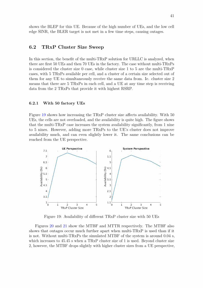
41

shows the BLEP for this UE. Because of the high number of UEs, and the low celledge SINR, the BLER target is not met in a few time steps, causing outages.

6.2 TRxP Cluster Size Sweep

In this section, the benefit of the multi-TRxP solution for URLLC is analyzed, whenthere are first 50 UEs and then 70 UEs in the factory. The case without multi-TRxPsis considered the cluster size 0 case, while cluster size 1 to 5 are the multi-TRxPcases, with 5 TRxPs available per cell, and a cluster of a certain size selected out ofthem for any UE to simultaneously receive the same data from. Ie. cluster size 2means that there are 5 TRxPs in each cell, and a UE at any time step is receivingdata from the 2 TRxPs that provide it with highest RSRP.

6.2.1 With 50 factory UEs

Figure 19 shows how increasing the TRxP cluster size affects availability. With 50UEs, the cells are not overloaded, and the availability is quite high. The figure showsthat the multi-TRxP case increases the system availability significantly, from 1 nineto 5 nines. However, adding more TRxPs to the UE’s cluster does not improveavailability much, and can even slightly lower it. The same conclusions can bereached from the UE perspective.

Figure 19: Availability of different TRxP cluster size with 50 UEs

Figures 20 and 21 show the MTBF and MTTR respectively. The MTBF alsoshows that outages occur much further apart when multi-TRxP is used than if itis not. Without multi-TRxPs the simulated MTBF of the system is around 0.04 s,which increases to 45.45 s when a TRxP cluster size of 1 is used. Beyond cluster size2, however, the MTBF drops slightly with higher cluster sizes from a UE perspective,

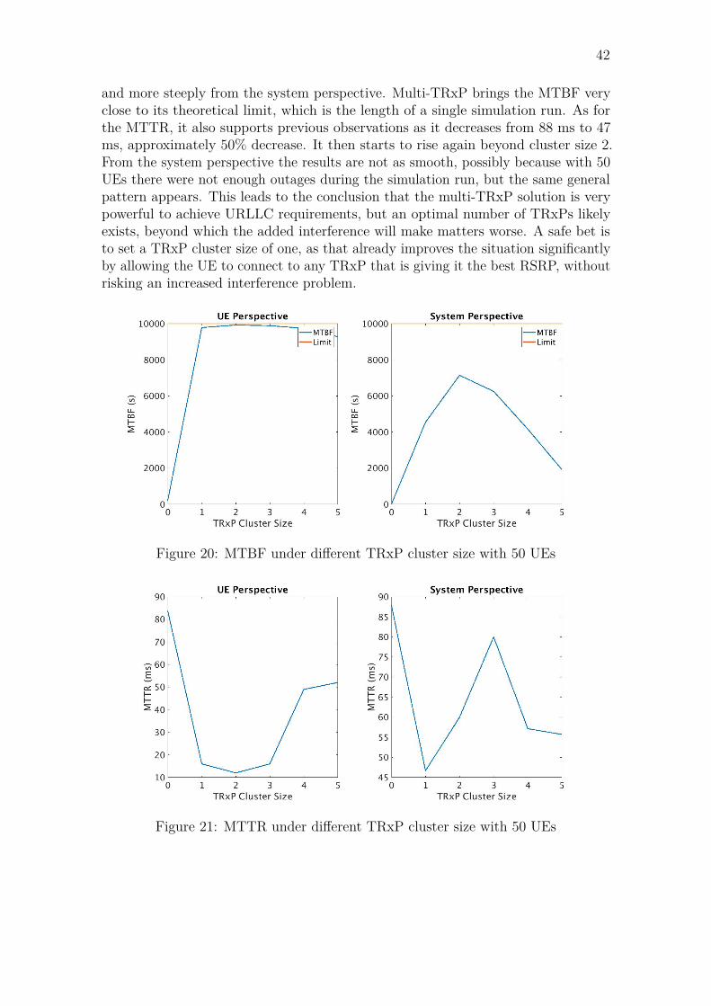
42

and more steeply from the system perspective. Multi-TRxP brings the MTBF veryclose to its theoretical limit, which is the length of a single simulation run. As forthe MTTR, it also supports previous observations as it decreases from 88 ms to 47ms, approximately 50% decrease. It then starts to rise again beyond cluster size 2.From the system perspective the results are not as smooth, possibly because with 50UEs there were not enough outages during the simulation run, but the same generalpattern appears. This leads to the conclusion that the multi-TRxP solution is verypowerful to achieve URLLC requirements, but an optimal number of TRxPs likelyexists, beyond which the added interference will make matters worse. A safe bet isto set a TRxP cluster size of one, as that already improves the situation significantlyby allowing the UE to connect to any TRxP that is giving it the best RSRP, withoutrisking an increased interference problem.

Figure 20: MTBF under different TRxP cluster size with 50 UEs

Figure 21: MTTR under different TRxP cluster size with 50 UEs

43

6.2.2 With 70 factory UEs

Figure 22 shows that the availability follows the same pattern as in the 50 UE case,but with a sharper drop in availability when more TRxPs than one are added to theUE cluster. This can be explained by the higher interference and lower availableresources, causing more outages. It is evident from the figure that receiving datafrom all available TRxPs is almost as bad as the situation when no TRxPs arepresent at all, when the cell is loaded. By comparing the availability from the 50 UEand 70 UE cases, it is clear that multi-TRxP can also allow for higher capacity in afactory, given a certain desired availability. From a UE perspective, for example, 3nines can be achieved even without TRxPs with a lower load (50 UEs), but with ahigher load (70 UEs), multi-TRxPs with a cluster size of 1 or 2 is needed to get thatlevel of availability.

Figure 22: Availability of different TRxP cluster size with 70 UEs

The results of the MTBF and MTTR show that the same affect occurs forreliability as in availability, as evident from Figure 23 and Figure 24 respectively.The system MTBF increases from 0.08 s to 76.82 s, when multi-TRxP is added withcluster size 1. However, it quickly drops to 4.51 s even as one more TRxP is addedto a cluster. Similarly, the system MTTR decreases from 9536 ms to 112 ms fromcase 0 and case 1, and then starts to rise again. The SINR plot in Figure 25 showsthat indeed, the overall SINR of all UEs improves significantly when multi-TRxPsare used, but then starts to decrease with each additional TRxP in the cluster, dueto the additional interference.

44

Figure 23: MTBF under different TRxP cluster size with 70 UEs

Figure 24: MTTR under different TRxP cluster size with 70 UEs

Figure 25: SINR for different TRxP cluster sizes with 70 UEs

45

6.2.3 With Variable Capacity

To further examine the effect of capacity on the factory’s performance, systemavailability for a range of number of UEs and over a range of TRxP cluster sizes isanalyzed. The results shown in Figure 26 support the previous observation that theavailability is highly dependant on the number of users. When the number of usersis lower than 50, outages are very rare. For instance, with 30 UEs, no outages wererecorded for any of the multi-TRxP cases. However without TRxPs, a few outageswere recorded even with 30 UEs, and the achieved system availability was close to 3nines. On the other hand, when 50 UEs are in the factory, the interference is largeenough so that better observations can be made by the study, while still having acomparatively decent level of availability. The 70 UEs case suffers from occasionalcongestion and discards, and therefore a significant drop in availability. This justifiedthe usage of 50 UEs and 70 UEs as the basis for analysis for most of the results, andreconfirms the ability of multi-TRxPs to improve availability and allow for largercapacity.

Figure 26: Availability of different TRxP cluster size with different number of UEs

6.3 Number of Existing TRxPs per cell Sweep

The second researched theme is whether or not the number of existing TRxPs inthe factory cell affects availability and reliability. For this part of the analysis, theTRxP cluster size is fixed to 2 TRxPs per UE, and number of existing TRxPs isswept from 2 to 7. Other parameters are kept the same.

46

6.3.1 With 50 factory UEs

Figure 27 shows that the with a fixed cluster size, the availability increases as thenumber of existing TRxPs in a cell increase. In fact, with 6 or 7 TRxPs, therewere no outages in the entire long simulation run, across any of the 5 experiments.Therefore, no results were added from those sweep values in the figure. This resultscan be justified when considering that the interference does not increase when thenumber of TRxPs increases, if the UE is only receiving data from a small numberof them. The additional existing TRxPs only help the UE select the two TRxPswhich can provide it with a higher signal, potentially because the increased numberof them means there is a higher likelihood of one being very close to the UE.

Figure 27: Availability under different number of available TRxPs per cell and 50UEs

Similar results can be observed from the MTBF in Figure 28, which also increasesand reaches the limit (the length of a single simulation run) with more existingTRxPs. The MTTR also generally decreases with more TRxPs, as shown in Figure29, eventually reaching 0 with 6 and 7 TRxPs as no outages are observed across anyof the simulation runs. Because the number of outages that could be obtained fromthe simulation was quite low, the decrease in MTTR is not consistent, and there aresome fluctuations. However with the available resources and time limitations, longenough simulations could not be run, as they might even require weeks of wall-clocktime in order to get a good statistical confidence with such a high availability, andseparate tools that are capable of analyzing such a massive amount of data.

6.3.2 With 70 factory UEs

Similar observations can be drawn from the 70 UE cases, but with a lower overallreliability and availability. Figure 30 shows that almost a linear relationship exists

47

Figure 28: MTBF under different number of available TRxPs per cell and 50 UEs

Figure 29: MTTR under different number of available TRxPs per cell and 50 UEs

between the number of existing TRxPs and availability as number of 9s. With 2existing TRxPs, and 70 UEs, the BLER target was not met by at least one UE in mosttime steps, corresponding to a system availability of as low as 1.72%. By increasingthe number of existing TRxPs per cell to 7, the system availability increases to99.95%, or 3 nines. This corresponds to a slope of (0.9995 − 0.0172)/(7 − 2) = 19.7%increase in system availability per added TRxP in a cell, on average. Similarly,increasing the number of existing TRxPs increases the MTBF and decreases theMTTR, as shown in Figure 31 and Figure 32 respectively.

48

Figure 30: Availability under different number of available TRxPs per cell and 70UEs

Figure 31: MTBF under different number of available TRxPs per cell and 70 UEs

Figure 32: MTTR under different number of available TRxPs per cell and 70 UEs

49

6.4 TRxP Ring Radius Sweep

In this section, the importance of where the TRxPs are placed around a cell isanalyzed. To simplify the analysis, the TRxPs are always placed as one in the middleof the cell, and others in a ring around it. The radius of this ring is varied in order toget an idea about whether or not an optimal placement exists. For those simulations,there were 5 existing TRxPs per cell, and a cluster size of 2 TRxPs per UEs, otherparameters are kept the same.

6.4.1 With 50 factory UEs

When the factory load is low, and outages are scarce, and the TRxP placementdoes not have a drastic effect on the KPIs. It appears that increasing the radius,which moves TRxPs of different cells closer together, slightly worsens the availability,MTBF and MTTR, as observed from Figure 33, Figure 34, and Figure 35 respectively.Even though this worsening is clear, it is important to properly inspect the axes,which clearly show that the reliability and availability remain quite high and the dropis not significant. Note that with radius 10 m there were no outages and thereforeno corresponding value in the availability plot.

Figure 33: Availability with different TRxP Ring Radius and 50 UEs

6.4.2 With 70 factory UEs

More meaningful results are observed from a more loaded cell, as there are moreoutages and the placement of TRxPs has a bigger impact on them. The resultsindicate that an optimal placement of TRxPs within the factory that results in thebest KPIs does likely exist. From Figure 36, it is clear that the best availability is

50

Figure 34: MTBF with different TRxP Ring Radius and 50 UEs

Figure 35: MTTR with different TRxP Ring Radius and 50 UEs

achieved when the surrounding TRxPs are 30 m away from the central TRxP. Thisfollows the conclusions made regarding the effects of interference on the scenario.When the TRxPs are too close to each other at the center of the cell, the benefitfrom their existance is minimal, as the spatial diversity gains are small. When theyare moved further apart, and cover more parts of the factory, they likelihood of aTRxP being close to a UE increases, and there is a higher chance that a UE’s SINRwill improve. However, when the TRxPs ring radius becomes higher than 30, thismeans that the TRxPs close to cell edge get very close to each other, keeping inmind that the linear distance between the center of the cells in the factory is 100 m.This increases the interference on users, causing more frequent and longer outages,as shown from the MTBF and MTTR in Figure 37 and 38 respectively.

51

Figure 36: Availability with different TRxP Ring Radius and 70 UEs

Figure 37: MTBF with different TRxP Ring Radius and 70 UEs

6.5 System Statistics and Confidence Intervals

Some statistics from the system perspective are displayed in Table 7. The tabledisplays the MTBF and MTTR with their corresponding 95% confidence intervalswith a normal distribution assumption, as the lower Confidence Limit (CL) andupper CL. The number of outage events is also shown. The results show that whenthe conditions are good and availability is high, the confidence intervals are quitelarge. This is expected, since the means are calculated from very few outage events.In some conditions there were no outages across the entire simulation run for any ofthe users across any of the experiments. For those cases a Not a Number (nan) ispresent in place of a confidence interval. Low statistical confidence is normal andexpected for high availability studies. For example, for the TRxP Cluster Size sweep,value 2, with 50 UEs, there were only 2 outage events from 5 different experiments,

52

Figure 38: MTTR with different TRxP Ring Radius 70 UEs

each with 50 users moving around the factory for 1 million time steps (plus 200 timesteps as a warmup period). The only way to achieve good statistical confidence insuch cases would be to have a different, faster simulation tool, less time limitation,as well as a better available tool for analyzing massive volumes of data. Alreadywith this data the post processing and plotting of figures took a very long time onMatlab, even after many code optimizations. The statistical confidence is howeverenough to compare results across different sweep values, and get valuable insight intohigh reliability studies and the optimal usage of the multi-TRxP solution. This isespecially true since the same overall conclusions were generally drawn from the 50UE and 70 UE cases, and the 70 UE cases generally have small confidence intervalsdue to more outages caused by the overloaded cells and increased interference.

53

Table 7: System Output StatisticsMTBF(s)

MTBFLowerCL

MTBFUpperCL

MTTR(ms)

MTTRLowerCL

MTTRUpperCL

OutageEvents

TRxPClusterSize

50 UEs

0 0.04 0.04 0.04 87.9 86.7 89.1 112041 45.45 19.42 71.49 46.7 13.7 79.6 62 71.43 32.34 110.52 60 -194.1 314.1 23 62.5 27.58 97.42 80 -82.9 242.9 34 41.67 17.04 66.29 57.1 0 114.3 75 19.23 10.59 27.87 55.7 33.1 78.4 21

TRxPClusterSize

70 UEs

0 0.08 0.05 0.11 9536.3 6121.1 12951.6 1041 76.82 5.5 148.14 111.7 42.9 180.4 122 4.51 3.09 5.94 139.7 101.8 177.7 2143 0.78 0.65 0.92 235.6 201.3 269.9 9804 0.37 0.31 0.42 478.2 406.8 549.6 11835 0.23 0.19 0.27 1053.5 852.8 1254.2 780

N.ExistingTRxPs

50 UEs

2 27.55 25.02 30.08 79.1 76.3 81.9 18053 746.23 243.92 1248.54 39.2 32.2 46.2 624 1515.11 935.65 2094.57 47.1 30.1 64.2 285 7142.84 3234 11051.68 60 -194.1 314.1 26 10000 10000 10000 0 nan nan 07 10000 10000 10000 0 nan nan 0

N.ExistingTRxPS

70 UEs

2 0.1 0.07 0.12 5552.3 3546.5 7558.1 1773 0.45 0.38 0.51 327.6 284.7 370.6 12944 1.77 1.39 2.14 148.5 123.9 173 5215 4.51 3.09 5.94 139.7 101.8 177.7 2146 58.67 11.58 105.77 160 7.2 312.8 167 124.94 11.99 237.88 74.3 40.2 108.4 7

54

MTBF(s)

MTBFLowerCL

MTBFUpperCL

MTTR(ms)

MTTRLowerCL

MTTRUpperCL

OutageEvents

TRxPRingRadius

50 UEs

10 10000 10000 10000 0 nan nan 020 7500 1995.94 13004.05 2 nan nan 130 5999.98 299.09 11700.86 6 -19.41 31.41 240 483.83 281.01 686.64 4.63 3.77 5.48 5945 576.86 413.49 740.23 6.43 5.04 7.82 49

TRxPRingRadius

70 UEs

10 0.34 0.29 0.4 24.95 21.47 28.42 107020 1.02 0.81 1.24 15.12 12.33 17.92 45530 2.26 1.54 2.97 13.97 10.18 17.77 21440 0.55 0.45 0.65 18.73 16.05 21.41 78050 0.2 0.17 0.23 40.54 34.9 46.18 1245

55

7 Conclusion

7.1 Summary

By means of simulations, a factory with mobile robots and two indoor cells isanalyzed, in order to observe how multi-TRxPs can be used to improve reliabilityand availability. First, the simulation shows that DCHO and MMIB-based LA can beused to eliminate successful HO interruption times, and reduce HO failures and RLFs.For all simulated cases, with medium (50 UEs) and slightly high (70 UEs) load on thefactory in terms of number of UEs, there were no recorded RLFs. However, outagesdefined by bad QoS periods still exist, and are quantified as the time steps when theLA cannot meet the BLER target for at least one UE. Outages occur mostly whenthe interference is high, and when the cell is too congested. Then, the ability to usemulti-TRxPs to decrease the outage durations and frequency is analyzed.

The simulation results show that for the case with multi-TRxPs, when a smallcluster size is chosen (1 or 2 TRxPs), availability, MTTR, and MTBF could besignificantly improved as compared to the case with no TRxPs. However, especiallywith a more loaded cell, further increasing the TRxP cluster size has a negativeeffect, due to the additional interference it causes. Regarding the number of TRxPsthat exist in a factory, it was shown that deploying more TRxPs generally improvesreliability and availability, for a fixed small TRxP cluster size. This is because theprobability of increasing the received power at a UE becomes higher when moreTRxPs exist, improving the SINR. Therefore, the general recommendation is todeploy many TRxPs, but have the UE receive data from only one or maximum twoat a time. This also allows a factory to increase its capacity, in terms of the numberof UEs, and still meet URLLC requirements.

Regarding the placement of TRxPs around the factory, it is found that it doesindeed have a large impact on reliability and availability, but only when the cellsare quite loaded and interference is already problematic. Then, an optimal positionexists where the TRxPs are distributed enough in the factory so that there is ahigher probability of them being near a UE at any time, thereby providing it with ahigher signal power, but still far enough from the TRxPs of the other cell so thatthe interference it causes is limited.

Finally, it is observed that the shadowing map does not have a significant impact onthe results, and simulation runs with different experiments corresponding to differentshadowing realizations produce very similar results with all other parameters keptconstant. Therefore, the displayed results have been averaged over the differentexperiments when present, and the results are therefore applicable to any factory,regardless of its associated shadowing realization.

56

7.2 Evaluation and Limitations

As with any simulation work, many limitations and sources of inaccuracies and errorscan exist, and it is vital to know what they are and how they affect the results.

To begin with, very strict requirements have been assumed, which might notactually be needed in a real application. Those strict requirements include not allowingany HARQ re-transmissions, which actually depends on the latency requirements ofthe application. Additionally, the outage definition is very strict. The applicationcould very likely tolerate a short time interval with few UEs having higher thantarget BLEP without any problems. This period of time during which the applicationwhich is consuming the communication service is able to continue its operation evenwithout an anticipated message is defined as survival time, according to TS 22.261[19]. Survival time has not been taken into account in this study, as it would havebeen difficult to come up with accurate values. Instead, a strict approach was takenwhere it is simply assumed to be zero. For this reason, the statistics for reliabilityand availability that were obtained are likely worse than what they actually wouldbe in reality.

Some limitations of the simulation tool includes that it does not model SDUsexplicitly, and therefore outage durations could not be observed from the SDUs thatwere not delivered correctly, in-time, and within QoS requirements. Instead, poorQoS has been linked to probability distributions, which is less accurate. Additionally,the tool’s timestep is 10 ms, which is quite large compared to TTI, and everythingwithin this time step is averaged, assuming a constant channel within it. This meansthat the smallest outage that could be recorded was 10 ms, when in fact it might bemuch shorter.

Overall, the simulation includes a large amount of abstraction, averaging, andsimplified models. One of the simplifications that likely had a large effect on theresults is the scheduling assumption. Any UE that cannot be served by its serving cellin a time step because all available PRBs are allocated, is considered ’discarded’, andremains so until a time step where the cell has enough resources after serving all otherUEs to serve it. The discarded UE is chosen randomly, when the available resourcesare lower than the required ones. Time steps for a discarded UE are considered tohave BLEP of 1, and are therefore in outage. This means that the outage durationfor a UE is much larger when it is discarded than what would realistically happen,where the UE would be served and another would be discarded in place of it. Thisaffects the UE perspective results, but not the system perspective ones, as thosewould be the same no matter which UE is in outage, as long as any is in outage.

Moreover, for all simulations, the fast fading standard deviation is taken as aconstant value, without taking into account the effect that the number of TRxPs wouldhave on it. Additionally, a global SINR standard deviation is assumed regardlessof the line of sight conditions. Additionally, the interference calculation is based on

57

load information from the previous time step, and is therefore not entirely accurate.BLEP values also fluctuate rapidly due to the spacing of the MCSs in the table, andthe fact that a new one can be selected at any time step. This affects the accuracyof the outage statistics. The LA is also reactive, and affected by the errors from UEreport delays, which are modelled.

The channel model used, which is a measurement-based industrial indoor channelmodel from [21] also introduces inaccuracies. Results from field measurements arealways at least partly specific to the conditions in which they were carried out.For a factory with different clutter or setup, the pathloss might be different. Themeasurements are also specific to the height difference between the transmitter andreceiver. The same difference has been used in the simulation as in the paper, butthe results are likely to differ for a different setup. Since the measurements are onlyvalid up to 140 m between Tx and Rx, the modeled factory size has been limited so asnot to exceed this distance. Additionally, human errors in making the measurementsare unavoidable, even when great care is taken. A cart was pushed forward at alow speed to gather samples of received power, and the person pushing the cartmust have varied his/her speed slightly and even moved slightly out of path at times.However, by having a large enough number of samples, this inaccuracy decreases,and the authors managed to achieve acceptable confidence intervals.

The paper provides both a path loss model with a fixed intercept as well as onewith a non-fixed intercept for the channel model. The authors point out that existingmodels from literature have usually used a fixed intercept path loss, such as [39] and[40]. Fixed intercepts assume that at the reference distance d0, path loss follows freespace propagation. This assumption does not fit the modeled scenario, as it is usuallyonly applicable in obstruction-free spacious areas with a very high Tx. Therefore,the non-fixed intercept pathloss, which has been adopted in this work, is moresuitable. The authors also verify their model by means of a Kolmogorov-Smirnov(K-S) goodness-of-fit test, and all the non-fixed intercept models passed the test atα = 0.5 level of significance. Additionally, the chosen pathloss exponent for this workis lower than the free space pathloss of n = 2, which is a good choice considering theheavy multipath propagation of the studied industrial environment. The authors alsomeasure the background radiation before starting their experiments, to guaranteethat machinery or other sources of noise does not disrupt their measurements.

Finally, an important limitation for this work is the time and resources limitation,which prevented the ability of running longer simulations and getting more precisestatistics. For all those reasons, as well as the inherent inaccuracy of reliabilitypredictions, and problems associated with the MTBF metric and its unrealisticunderlying assumptions, the absolute results should not be taken as an accurateassessment of the reliability level of a similar factory scenario in reality. Instead, theresults give valuable insight into the relative difference of the design choices.

58

7.3 Future Work

This work is seen as a starting point, on top of which many other aspects could beanalyzed if time permits. An important aspect to analyze would be the combinationof beamforming with the multi TRxP solution. Beamforming is a key feature of 5G,and an excellent method to reduce interference. Interference could also be reducedby means of interference coordination and mitigation techniques, such as eICIC.Another possibility is to utilize the scenario to study the impact of predictive mobility,where the HO decisions are made via a Machine Learning (ML) algorithm which istrained under similar industrial conditions. ML can be potentially used to optimizethe triggers and offsets, and to connect to the best cell in order to attempt to keepthe SINR high.

Further improvements could include modeling the control plane, and observinghow it performs. Control plane signals can tolerate higher delays and therefore HARQre-transmissions could potentially be used, which would improve the reliability. Itwould also be interesting to study the time distribution of errors, to see if outagesare occurring in bursts or more regularly, for example. Outages caused by a badhandover or multi-TRxP decision will probably be correlated in time. This wouldrequire a much longer simulation run in order to be properly analyzed. The spatialdistribution of errors can also be studied, to see if there are certain areas of thefactory where UEs are more likely to experience outages. Moreover, the factory’sperformance under mixed traffic models can be analyzed, with both best effort mobilebroadband background users, as well as the URLLC traffic.

In order to improve the errors caused by UE reports, the link adaptation canbe made to consider the CQI reporting delays while the MCS is being selected.This can be achieved by providing the scheduler with additional information, suchas the channel variations and delay [34]. Additionally, more accurate estimatesof the channel quality can be obtained if the UE is made to report the PUCCHmore frequently, which comes at the expense of higher signaling overhead and powerconsumption [38].

Longer simulation runs and more experiments can be conducted to improve thestatistical confidence, but could lead to an unreasonably long waiting time andunreasonably large collected data, which would require a separate tool that is capableof analyzing the data and producing the required plots. Different aspects couldalso be analyzed if time permits, such as having more simulations while sweepingthe number of factory UEs. The effect of the placement of TRxPs could also bestudied by considering all different locations around the factory, instead of assuminga circular placement and only varying the radius. Moreover, different multi-pointtransmission methods could also be compared, such as analyzing dynamic pointselection, as it might be a better method considering the large impact of interference.Additionally, for the DCHO, different TTT and offsets could be considered, andresults with FCS could also be observed and compared to DD.

59

References

[1] E. Dahlman, et al. "5G Wireless Access: Requirements and Realization". IEEECommunications Magazine, vol. 52, no. 12, pp.42 - 47, December 2014.

[2] M. Luvisotto, Z. Pang, and D. Dzung, "Ultra High Performance WirelessControl for Critical Applications: Challenges and Directions," IEEE Transactionson Industrial Informatics, vol. 13, no. 3, pp. 1448-1459, June 2017

[3] "Global Industrial Wireless Sensor Network Market to Reach Nearly US$ 7,000Mn in Revenues by 2026-end", Persistent Market Research, Mar 19, 2018.Available: https://www.persistencemarketresearch.com/mediarelease/industrial-wireless-sensor-network-market.asp

[4] S. A. Ashraf, I. Aktas, E. Eriksson, K. W. Helmersson and J. Ansari,“Ultra-reliable and low-latency communication for wireless factory automation:From LTE to 5G”, IEEE International Conference on Emerging Technologiesand Factory Automation (ETFA), Sept. 2016.

[5] N. Larson, et al., "Investigating Excessive delays in mobile broadband networks,"Proc. ACM Sigcom, 2015.

[6] B. Holfeld, et al. "Wireless Communication for Factory Automation: anopportunity for LTE and 5G systems," IEEE Communications Magazine, vol.54, no. 6, pp. 36-43, June 2016.

[7] American Society for Quality (ASQ). 2011. Glossary: Reliability. Accessed onAugust 01, 2018. Available at http://asq.org/glossary/r.html.

[8] 3GPP TR 22.804: "Technical Specification Group Services and System Aspects;Study on Communication for Automation in Vertical Domains", 2018.

[9] IEC 61907: "Communication network dependability engineering", 2009.

[10] 3GPP TS 38.401: "Technical Specification Group Radio Access Network; NG-RAN", 2018.

[11] 3GPP TR 38.913: "Study on Scenarios and Requirements for Next GenerationAccess Technologies", 2018.

[12] A. Elnashar and M. A. El-Saidny, "Looking at LTE in Practice: A PerformanceAnalysis of the LTE System Based on Field Test Results," in IEEE VehicularTechnology Magazine, vol. 8, no. 3, pp. 81-92, Sept. 2013.

[13] S. Barbera, et al. "Synchronized RACH-less handover solution for LTE het-erogeneous networks," International Symposium on Wireless CommunicationSystems (ISWCS), Brussels, 2015, pp. 755-759.

60

[14] I. Viering, H. Martikainen, A. Lobinger and B. Wegmann, "Zero-Zero Mobility:Intra-Frequency Handovers with Zero Interruption and Zero Failures," in IEEENetwork, vol. 32, no. 2, pp. 48-54, March-April 2018.

[15] L. Wan, S. Tsai and M. Almgren, "A Fading-Insensitive Performance Metric fora Unified Link Quality Model," IEEE Wireless Communications and NetworkingConference, 2006. WCNC 2006., Las Vegas, NV, 2006, pp. 2110-2114.

[16] 3GPP TS 38.214: "Technical Specification Group Radio Access Network; NR;Physical layer procedures for data", 2018.

[17] E. Ackerman, “Brad Porter, VP of Robotics at Amazon, on Ware-house Automation, Machine Learning, and His First Robot.” IEEE Spec-trum: Technology, Engineering, and Science News, IEEE Spectrum, 27 Sept.2018. Available at: ieee.org/automaton/robotics/industrial-robots/interview-brad-porter-vp-of-robotics-at-amazon.

[18] Allied Market Research, "Global Warehouse Robotics Market - Segmentedby Type, Function, End-user Industry (E-commerce, Automotive, Food andBeverage, Chemical, Electrical, Paper, Textile), and Region - Growth, Trends,and Forecast (2018 - 2023)", 14 May, 2018.

[19] 3GPP TS 22.261: "Technical Specification Group Services and System Aspects;Service requirements for the 5G system", 2018.

[20] N. Brahmi, O. N. C. Yilmaz, K. W. Helmersson, S. A. Ashraf and J. Torsner,"Deployment Strategies for Ultra-Reliable and Low-Latency Communication inFactory Automation," IEEE Globecom Workshops (GC Wkshps), San Diego,CA, 2015, pp. 1-6.

[21] E. Tanghe et al., "The industrial indoor channel: large-scale and temporal fadingat 900, 2400, and 5200 MHz," in IEEE Transactions on Wireless Communications,vol. 7, no. 7, pp. 2740-2751, July 2008.

[22] M. Deruyck, J. Hoebeke, et al., "Intelligent TDMA heuristic scheduling bytaking into account physical layer interference for an industrial IoT environment",Telecommunication Systems, 2017.

[23] X. Gong, D. Plets, E. Tanghe, et al., "An efficient genetic algorithm forlarge-scale transmit power control of dense and robust wireless networks in harshindustrial environments", Applied Soft Computing, 2018.

[24] N. A. Johansson, Y. -. E. Wang, E. Eriksson and M. Hessler, "Radio accessfor ultra-reliable and low-latency 5G communications," IEEE InternationalConference on Communication Workshop (ICCW), London, 2015, pp. 1184-1189.

61

[25] G. Pocovi, B. Soret, M. Lauridsen, K. I. Pedersen and P. Mogensen, “Signalquality outage analysis for ultra-reliable communications in cellular networks”,IEEE Globecom Workshops, Dec. 2015.

[26] F. Kirsten, D. Ohmann, M. Simsek and G. P. Fettweis, “On the utilityof macro- and microdiversity for achieving high availability in wireless net-works”, IEEE International Symposium on Personal, Indoor and Mobile RadioCommunications, Sept. 2015.

[27] F. Salah, M. Rinne, "Performance Analysis of User Plane Connectivity in the5G Non-Standalone Deployment", to appear in IEEE Globecom, Dec. 2018.

[28] “Nokia 5G for Mission Critical Communication” Nokia, Espoo, Finland,2016. Available: http://www.hit.bme.hu/~jakab/edu/litr/5G/Nokia_5G_for_Mission_Critical_Communication_White_Paper.pdf

[29] 3GPP TR 38.802: "Study on New Radio Access Technology Physical LayerAspects", 2017.

[30] H. Shariatmadari, S. Iraji, R. Jantti, P. Popovski, Z. Li, and M. Uusitalo"Fifth-Generation Control Channel Design: Achieving Ultrareliable Low-LatencyCommunications," IEEE Vehicular Technology Magazine, 2018, 13(2), 84-93.

[31] D.M. Kim, P. Popovski, "Reliable Uplink Communication Through DoubleAssociation in Wireless Heterogeneous Networks," IEEE Wireless Commun.Letters, 2016, 5.3: 312-315.

[32] E. Dahlman, S. Parkvall, and J. Skold "4G, LTE-advanced Pro and the Roadto 5G". Academic Press, 2016. Chapter 13: Multi-Point Coordination andTransmission.

[33] T. Rappaport, "Wireless Communications Principals and Practice" , chapter 5:Mobile Radio Propagation: Small-Scale Fading and Multipath, 2001.

[34] U. Oruthota, F. Ahmed, and O. Tirkkonen, “Ultrareliable link adaptation fordownlink MISO transmission in 5G cellular networks,” Inform., vol. 7, no. 1,pp. 1–18, Mar. 2016.

[35] P. O’Connor, "Practical Reliability Engineering (Fourth Ed.)", John Wiley andSons, New York. ISBN 978-0-4708-4462-5, 2002.

[36] RCM II, "Reliability Centered Maintenance, Second edition" 2008, page 250-260,the role of Actuarial analysis in Reliability.

[37] "Why You Cannot Predict Electronic Product Reliability" 2012 ARS, Europe.Warsaw, Poland.

[38] C. She, C. Yang, and T. Q. S. Quek, “Radio resource management forultra-reliable and low-latency communications,” IEEE Commun. Mag., vol. 55,no. 6, pp. 72–78, 2017.

62

[39] T. Rappaport and C. McGillem, “UHF fading in factories,” IEEE J. Select.Areas Commun, vol. 7, no. 1, pp. 40–48, Jan. 1989.

[40] S. Kjesbu and T. Brunsvik, “Radiowave propagation in industrial environments,”in Proc. 26th Annual Conference of the IEEE Industrial Electronics Society, vol.4, pp. 2425–2430, Oct. 2000.

[41] B. Singh, Z. Li, O. Tirkkonen, M. A. Uusitalo and P. Mogensen, "Ultra-reliablecommunication in a factory environment for 5G wireless networks: Link level anddeployment study," IEEE 27th Annual International Symposium on Personal,Indoor, and Mobile Radio Communications (PIMRC), Valencia, 2016, pp. 1-5.