Multi-tier Store Brands and Channel Pro ts Technical Appendixbear.warrington.ufl.edu/wshin/Woochoel_Shin/SB_appendix.pdf · A3 where IN i is the indicator function taking the value

Multi-tier Store Brands and Channel Profits

Technical Appendix

1

Table of Contents

Equilibrium Solutions

Bilateral Monopoly

Lemma A1 (Equilibrium without Store Brand) A1

Lemma A2 (Equilibrium with Store Brand) A4

Lemma A3 (Two-Part Tariff without Store Brand) A7

Lemma A4 (Two-Part Tariff with Store Brand) A8

Lemma A5 (Store Brand Procurement from Manufacturer) A9

Lemma A6 (Store Brand with Lower Perceived Quality) A10

Lemma A7 (Retailer Moving First) A11

Manufacturer Competition



Lemma A10 (Retailer Moving First) A15

Retailer Competition



Lemma A13 (Retailers Moving First) A20

Proof of Propositions and Claims

Lemma A14 A22

Proposition 1 A23

Lemma A15 A24

Corollary A1 A25

Claims in Footnote 2 A26

Claims below Proposition 1 A26

Proposition 2 A27

Proposition 3 A28

Proposition 4 A30

Proposition 5 A30

Claims below Proposition 5 A30

Claims in Footnotes 8 and 9 A31

Claims in Section 3.6.1 A33





Claims above Proposition 6 A40

Proposition 6 A41



A1

In this Appendix, we first establish a series of lemmas on the equilibrium solutions for bilateral

monopoly model, retailer competition model, and manufacturer competition model. Then using

these lemmas, we prove the five propositions and the related claims. To help follow the proof, we

provide the summary of notation in Table A1.

Table A1. Summary of Notation

Notation Explanation

θ Consumers’ sensitivity to quality

a, b Lower and upper support of the distribution of θ

Nj index of the jth product in the pq order among the national brands (j = 1, . . . , J)

Sk index of the kth product in the pq order among the store brands (k = 1, . . . ,K)

i index of the ith product in the pq order among all products in the market (i = 1, . . . , I)

N , S Total numbers of national brands and store brands in the market

pNj , pSk Prices of national brand j and store brand k

qNj , qSk Qualities of national brand j and store brand k

wNj Wholesale price of national brand j

W Fixed fee charged for the national brand under two-part tariff

zNj , zSk Demands of national brand j and store brand k

ci Marginal cost to the retailer for product i

πM , πR Gross profits of the manufacturer and the retailer

ΠM , ΠR Net profits of the manufacturer and the retailer

jNkS Indicator for the scenario with j national brands and k store brands introduced

SS Indicator for the scenario where the manufacturer supplies the store brand

RS, RB Indicators for the retailer competition scenario with and without store brand

MS, MB Indicators for the manufacturer competition scenario with and without store brand

jNkS(T ) Indicator for the two-part tariff scenario with j national brands and k store brands

φ Index of the subcases in each scenario (φ = 1, . . . ,Φ)

q(φ)S (qNj ,∀j) Local best response function of the retailer to national brand qualities in subcase φ

q̃N , q̃S Vectors of national brand qualities and store brand qualities

∆Xq , ∆X

p Ranges of qualities and prices of all products in the market in Scenario X

CWX Consumer welfare in Scenario X

Equilibrium Solutions

Lemma A1 (Bilateral Monopoly without Store Brands). Suppose there is one manufacturer and

one retailer. Further suppose that the retailer sells national brands and does not offer any store

brand. The equilibrium qualities, prices and profits corresponding to the cases where the manufac-

turer sells one, two, three, four, or five national brands are as follows:

A2

Case qN1 qN2 qN3 qN4 qN5 pN1 pN2 pN3 pN4 pN5 πM πR

N=1 0.3333b N/A N/A N/A N/A 0.2778b2 N/A N/A N/A N/A 0.0185b3

b−a0.0093b3

b−aN=2 0.4000b 0.2000b N/A N/A N/A 0.3400b2 0.1600b2 N/A N/A N/A 0.0200b3

b−a0.0100b3

b−aN=3 0.4286b 0.2857b 0.1429b N/A N/A 0.3673b2 0.2347b2 0.1122b2 N/A N/A 0.0204b3

b−a0.0102b3

b−aN=4 0.4444b 0.3333b 0.2222b 0.1111b N/A 0.3827b2 0.2778b2 0.1790b2 0.0864b2 N/A 0.0206b3

b−a0.0103b3

b−aN=5 0.4545b 0.3636b 0.2727b 0.1818b 0.0909b 0.3926b2 0.3058b2 0.2231b2 0.1446b2 0.0702b2 0.0207b3

b−a0.0103b3

b−a

Proof. We first derive the general solution and then obtain the specific equilibrium pertaining for

the four cases presented in the above table. Recall that the sequence of decisions in this game is

as follows:

1. The manufacturer sets the quality of the national brands, qNj .

2. The manufacturer decides the wholesale price of the national brands, wNj .

3. The retailer sets the retail price of the national brands, pNj .

We solve the game backwards. In the last stage of the game, the retailer sets the retail price to

maximize its profits. The retailer’s profits given in equation (3) of the main paper can be rewritten

more generally as follows:

πR =(

1b−a

){(b− p1−p2

q1−q2

)(p1−c1)+

(p1−p2q1−q2

− p2−p3q2−q3

)(p2−c2)+···+

(pi−1−piqi−1−qi

− pi−pi+1qi−qi+1

)(pi−ci)+···

+

(pI−2−pI−1qI−2−qI−1

− pI−1−pIqI−1−qI

)(pI−1−cI−1)+

(pI−1−pIqI−1−qI

− pIqI

)(pI−cI)

}, (A1)

where i indicates the ith product in the order of price per unit quality (i.e., piqi ). Note that ci is the

marginal cost of the retailer, and it is wi for a national brand and q2i for a store brand. Since πR

is a concave function of each retail price, it follows from the first-order condition ∂πR∂pi

= 0, that we

have the following I equations:

b = (2p1−c1)−(2p2−c2)q1−q2 = · · · = (2pi−1−ci−1)−(2pi−ci)

qi−1−qi = · · · = (2pI−1−cI−1)−(2pI−cI)qI−1−qI = 2pI−cI

qI. (A2)

On simultaneously solving these equations, we obtain,

pi(wi, ci) = bqi+ci2 =

{bqi+wi

2 if i is the national brandbqi+q

2i

2 if i is the store brand. (A3)

Using the above solution, the manufacturer’s profit given in equation (2) of the main paper can be

rewritten as

πM =(

1b−a

){(b2− w1−w2

2(q1−q2)

)(w1−q21)IN1 +

(w1−w22(q1−q2)

− w2−w32(q2−q3)

)(w2−q22)IN2 +···+

(wi−1−wi2(qi−1−qi)

− wi−wi+12(qi−qi+1)

)(wi−q2i )INi +···

+

(wI−2−wI−12(qI−2−qI−1)

− wI−1−wI2(qI−1−qI )

)(wI−1−q2I−1)INI−1+

(wI−1−wI2(qI−1−qI )

− wI2qI

)(wI−q2I )INI

}, (A4)

A3

where INi is the indicator function taking the value of one if i is the national brand, but zero

otherwise. Note that in this lemma, INi = 1, ∀i. Furthermore, πM is also a concave function of each

wholesale price. Hence, from the first-order condition ∂πM∂wi

= 0, we have the following I equations:

b =(2w1−q21+bq1)−(2w2−q22+bq2)

2(q1−q2) = · · · = (2wi−1−q2i−1+bqi−1)−(2wi−q2i+bqi)

2(qi−1−qi) (A5)

= · · · = (2wI−1−q2I−1+bqI−1)−(2wI−q2I+bqI)

2(qI−1−qI) =2wI−q2I+bqI

2qI.

Upon simultaneously solving these equations, we obtain,

wi(qi) =bqi+q

2i

2 . (A6)

Given these solutions, the manufacturer’s unit margin from each product is wi − q2i =

bqi−q2i2 .

Moreover, because pi−pi+1

qi−qi+1= 3b+qi+qi+1

4 , the demand for each product is given by,

zi(qi, i = 1, . . . , I) =

b−qi−qi+1

4 if i = 1qi−1−qi+1

4 if i = 2, 3, . . . , I − 1qi−1

4 if i = I

. (A7)

Now we can rewrite the manufacturer’s profit as a function of qualities in the following way:

πM =(

1b−a

){(b−q1−q2)(bq1−q

21)

8+

(q1−q3)(bq2−q22)

8···+ (qi−1−qi+1)(bqi−q

2i )

8+···

+(qI−2−qI )(bqI−1−q

2I−1)

8+qI−1(bqI−q

2I )

8

}(A8)

Since πM is a concave function of each product’s quality, we can use the first-order conditions

∂πM∂qi

= 0 to obtain the following I equations:

qi =

b+qi+1

3 if i = 1qi−1+qi+1

2 if i = 2, 3, . . . , I − 1qi−1

2 if i = I

. (A9)

By simultaneously solving these equations, we obtain,

qi = (I−i+1)b2I+1 . (A10)

On plugging (A10) back into (A6) and then into (A3), we obtain the equilibrium prices given below

wi = (I−i+1)(3I−i+2)b2

2(2I+1)2(A11)

pi = (I−i+1)(7I−i+4)b2

4(2I+1)2. (A12)

Then, by (A7), the equilibrium demand is

zi = b2(2I+1)(b−a) . (A13)

A4

Finally, plugging in these solutions into (A8) and (A1) respectively, we obtain,

πM = I(I+1)b3

12(2I+1)2(b−a)(A14)

πR = I(I+1)b3

24(2I+1)2(b−a). (A15)

Finally, by plugging in the relevant I and i to the above general solutions, we obtain the specific

equilibrium prices, qualities and profits given in the lemma. (Note that in this lemma, I = N .)

Lemma A2 (Bilateral Monopoly with Store Brands). Suppose there is one manufacturer and

one retailer. The equilibrium solution for the following cases where the number of national brands

j = {1, 2, 3, 4} and the number of store brands k = {1, 2, 3} are as follows:

Case qN1 qN2 qN3 qN4 qS1 qS2 qS3 qS4 πM

N=1,S=1 0.1785b N/A N/A N/A 0.3449b N/A N/A N/A 0.0013b3

b−aN=1,S=2 0.1132b N/A N/A N/A 0.4044b 0.2131b N/A N/A 0.0003b3

b−aN=1,S=3 0.0829b N/A N/A N/A 0.4309b 0.2926b 0.1543b N/A 0.0001b3

b−aN=1,S=4 0.0653b N/A N/A N/A 0.4458b 0.3375b 0.2292b 0.1209b 0.0001b3

b−aN=2,S=1 0.4426b 0.1638b N/A N/A 0.3307b N/A N/A N/A 0.0018b3

b−aN=2,S=2 0.3133b 0.1047b N/A N/A 0.4087b 0.2050b N/A N/A 0.0005b3

b−aN=2,S=3 0.2361b 0.0791b N/A N/A 0.4335b 0.3004b 0.1513b N/A 0.0002b3

b−aN=3,S=1 0.4444b 0.2222b 0.1111b N/A 0.3333b N/A N/A N/A 0.0021b3

b−aN=3,S=2 0.4653b 0.2967b 0.0988b N/A 0.3980b 0.1988b N/A N/A 0.0006b3

b−aN=4,S=1 0.4451b 0.2515b 0.1677b 0.0838b 0.3342b N/A N/A N/A 0.0021b3

b−aCase pN1 pN2 pN3 pN4 pS1 pS2 pS3 pS4 πR

N=1,S=1 0.1126b2 N/A N/A N/A 0.2320b2 N/A N/A N/A 0.0376b3

b−aN=1,S=2 0.0659b2 N/A N/A N/A 0.2840b2 0.1293b2 N/A N/A 0.0401b3

b−aN=1,S=3 0.0463b2 N/A N/A N/A 0.3082b2 0.1891b2 0.0890b2 N/A 0.0409b3

b−aN=1,S=4 0.0357b2 N/A N/A N/A 0.3223b2 0.2257b2 0.1409b2 0.0678b2 0.0412b3

b−aN=2,S=1 0.3256b2 0.1022b2 N/A N/A 0.2201b2 N/A N/A N/A 0.0380b3

b−aN=2,S=2 0.2083b2 0.0605b2 N/A N/A 0.2878b2 0.1235b2 N/A N/A 0.0403b3

b−aN=2,S=3 0.1473b2 0.0441b2 N/A N/A 0.3107b2 0.1953b2 0.0871b2 N/A 0.0409b3

b−aN=3,S=1 0.3272b2 0.1420b2 0.0679b2 N/A 0.2222b2 N/A N/A N/A 0.0381b3

b−aN=3,S=2 0.3432b2 0.1948b2 0.0568b2 N/A 0.2782b2 0.1192b2 N/A N/A 0.0403b3

b−aN=4,S=1 0.3278b2 0.1626b2 0.1049b2 0.0507b2 0.2230b2 N/A N/A N/A 0.0381b3

b−a

Proof. The sequence of events in this game is as follows:

1. The manufacturer sets the qualities of the national brands, qNj .

2. The retailer sets the qualities of the store brands, qSj .

3. The manufacturer sets the wholesale prices of the national brands, wNj .

A5

4. The retailer sets the retail prices of all products, pNj and pSj .

We solve the game using backward induction. In the last stage of the game, the retailer’s profit

remains the same as given in equation (A1) and hence the optimal retail prices are given as in

equation (A3). Consequently, the manufacturer’s profits are as given in equation (A4). Now focus

on i which is a national brand. From the first-order condition with respect to wi, we obtain the

following:

• if i = 1:

b =(2w1−q21+bq1)−(2w2−q22+bq2)

2(q1−q2) (A16)

• if i = I:

(2wI−1−q2I−1+bqI−1)−(2wI−q2I+bqI)


2qI(A17)

• if 1 < i < I and both i− 1 and i+ 1 are national brands:

(2wi−1−q2i−1+bqi−1)−(2wi−q2i+bqi)

2(qi−1−qi) =(2wi−q2i+bqi)−(2wi+1−q2i+1+bqi+1)

2(qi−qi+1) (A18)

• if 1 < i < I and i− 1 a national brand but i+ 1 is a store brand:

(2wi−1−q2i−1+bqi−1)−(2wi−q2i+bqi)

2(qi−1−qi) =(2wi−q2i+bqi)−(q2i+1+bqi+1)

2(qi−qi+1) (A19)

• if 1 < i < I and i− 1 a store brand but i+ 1 is a national brand:

(q2i−1+bqi−1)−(2wi−q2i+bqi)

2(qi−1−qi) =(2wi−q2i+bqi)−(2wi+1−q2i+1+bqi+1)

2(qi−qi+1) (A20)

• if 1 < i < I and both i− 1 and i+ 1 are store brands:

(q2i−1+bqi−1)−(2wi−q2i+bqi)

2(qi−1−qi) =(2wi−q2i+bqi)−(q2i+1+bqi+1)

2(qi−qi+1) (A21)

Denote the index of the highest-quality store brand by h, and that of the lowest-quality store brand

by l. Then, for all national brands i satisfying qi > qh (that is, i < h), we have

b =(2w1−q21+bq1)−(2w2−q22+bq2)

2(q1−q2) = · · · = (2wi−q2i+bqi)−(2wi+1−q2i+1+bqi+1)

2(qi−qi+1) = · · · (A22)

=(2wh−2−q2h−2+bqh−2)−(2wh−1−q2h−1+bqh−1)

2(qh−2−qh−1) =(2wh−1−q2h−1+bqh−1)−(q2h+bqh)

2(qh−1−qh) .

Simultaneously solving these (h− 1) equations, we obtain

wi =q2i+q2h+b(qi−qh)

2 , (i ≤ h− 1). (A23)

A6

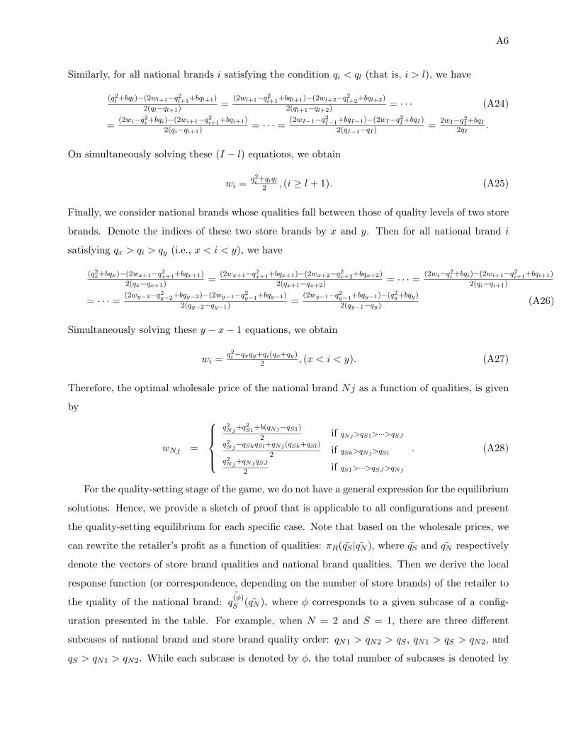
Similarly, for all national brands i satisfying the condition qi < ql (that is, i > l), we have

(q2l +bql)−(2wl+1−q2l+1+bql+1)

2(ql−ql+1) =(2wl+1−q2l+1+bql+1)−(2wl+2−q2l+2+bql+2)

2(ql+1−ql+2) = · · · (A24)

=(2wi−q2i+bqi)−(2wi+1−q2i+1+bqi+1)

2(qi−qi+1) = · · · = (2wI−1−q2I−1+bqI−1)−(2wI−q2I+bqI)


2qI.

On simultaneously solving these (I − l) equations, we obtain

wi =q2i+qiql

2 , (i ≥ l + 1). (A25)

Finally, we consider national brands whose qualities fall between those of quality levels of two store

brands. Denote the indices of these two store brands by x and y. Then for all national brand i

satisfying qx > qi > qy (i.e., x < i < y), we have

(q2x+bqx)−(2wx+1−q2x+1+bqx+1)

2(qx−qx+1) =(2wx+1−q2x+1+bqx+1)−(2wx+2−q2x+2+bqx+2)

2(qx+1−qx+2) = · · · = (2wi−q2i+bqi)−(2wi+1−q2i+1+bqi+1)

2(qi−qi+1)

= · · · = (2wy−2−q2y−2+bqy−2)−(2wy−1−q2y−1+bqy−1)

2(qy−2−qy−1) =(2wy−1−q2y−1+bqy−1)−(q2y+bqy)

2(qy−1−qy) (A26)

Simultaneously solving these y − x− 1 equations, we obtain

wi =q2i−qxqy+qi(qx+qy)

2 , (x < i < y). (A27)

Therefore, the optimal wholesale price of the national brand Nj as a function of qualities, is given

by

wNj =

q2Nj+q

2S1+b(qNj−qS1)

2 if qNj>qS1>···>qSJq2Nj−qSkqSl+qNj(qSk+qSl)

2 if qSk>qNj>qSlq2Nj+qNjqSJ

2 if qS1>···>qSJ>qNj

. (A28)

For the quality-setting stage of the game, we do not have a general expression for the equilibrium

solutions. Hence, we provide a sketch of proof that is applicable to all configurations and present

the quality-setting equilibrium for each specific case. Note that based on the wholesale prices, we

can rewrite the retailer’s profit as a function of qualities: πR(q̃S |q̃N ), where q̃S and q̃N respectively

denote the vectors of store brand qualities and national brand qualities. Then we derive the local

response function (or correspondence, depending on the number of store brands) of the retailer to

the quality of the national brand:˜q

(φ)S (q̃N ), where φ corresponds to a given subcase of a config-

uration presented in the table. For example, when N = 2 and S = 1, there are three different

subcases of national brand and store brand quality order: qN1 > qN2 > qS , qN1 > qS > qN2, and

qS > qN1 > qN2. While each subcase is denoted by φ, the total number of subcases is denoted by

A7

Φ. Now the best response function/correspondence is given by,

q̃S(q̃N ) =

˜q

(1)S (q̃N ) if πR(

˜q

(1)S (q̃N )) ≥ πR(

˜q

(φ)S (q̃N )),∀φ

˜q

(2)S (q̃N ) if πR(

˜q

(2)S (q̃N )) ≥ πR(

˜q

(φ)S (q̃N )),∀φ

· · ·˜q

(Φ)S (q̃N ) if πR(

˜q

(Φ)S (q̃N )) ≥ πR(

˜q

(φ)S (q̃N )),∀φ

(A29)

Given this best response function/correspondence as well as the prices derived above, the man-

ufacturer’s profits can be rewritten as a function of national brand qualities only: πM (q̃N ). On

maximizing this profit, we obtain the optimal qualities of national brands: q̃N∗. Depending on the

subcase that this solution falls on (say, it is Case φ), we plug in the optimal national brand qualities

into the relevant local best response function/correspondence and obtain the optimal qualities of

the store brands:˜q

(φ)S

∗=

˜q

(φ)S (q̃N

∗).

On plugging these optimal qualities into equation (A28), we obtain the optimal wholesale prices

of national brands: w∗Nj . Then we get the optimal retail prices of all products by plugging the

optimal wholesale prices into equation (A3). Finally, the optimal profits can be obtained using

equations (A1) and (A4).

Lemma A3 (Bilateral Monopoly: Two-Part Tariff with No Store Brand). Suppose there is one

manufacturer and one retailer in the channel offering one national brand. When the manufac-

turer charges both the per-unit wholesale price and the lump-sum fixed fee (W ) to the retailer, the

equilibrium solution for this case is given by:

q1N(T )N = 0.3333b, w

1N(T )N = 0.1111b2,W 1N(T ) = 0.0370b3

b−a , p1N(T )N = 0.2222b2, (A30)

z1N(T )N = 0.3333b

b−a , π1N(T )M = 0.0370b3

b−a , π1N(T )R = 0

Proof. The order of events in this game is as follows:

1. The manufacturer decides the quality of the national brand, qN .

2. The manufacturer sets the wholesale price wN and the fixed fee W , for the national brand.

3. The retailer sets the retail price of the national brand pN .

First, the gross profits of the two firms are given as,

πM =(

1b−a

)(b− pN

qN

)(wN − q2

N ) +W (A31)

πR =(

1b−a

)(b− pN

qN

)(pN − wN )−W. (A32)

A8

Since the fixed fee does not affect the first-order condition ( ∂πR∂pN= 0), the optimal retail price is

given as in (A3), by pN = bqN+wN2 . Given this, the profits are revised as,

πM (wN ,W ) =(bqN−wN )(wN−q2N )

2(b−a)qN+W (A33)

πR(wN ,W ) = (bqN−wN )2

4(b−a)qN−W. (A34)

Since ∂πM (wN ,W )∂W > 0, ∀wN and the retailer should earn non-negative profits (i.e., πR(wN ,W ) ≥ 0),

the optimal fixed fee is given as W ∗ = (bqN−wN )2

4(b−a)qN. Given this, the manufacturer sets wN from the

first-order condition ∂πM (wN ,W∗)

∂wN= 0. Thus we obtain wN = q2

N . Finally, the manufacturer sets

the optimal quality qN by maximizing the following profits:

πM (qN ) = qN (b−qN )2

4(b−a) . (A35)

Then it is easy to see that the optimal quality is given as qN = 0.3333b. Based on this, we have

wN = q2N = 0.1111b2 and pN = 0.2222b2, and the rest of the results follow.

Lemma A4 (Bilateral Monopoly: Two-Part Tariff with the Store Brand). Suppose there is one

manufacturer and one retailer in the channel offering one national brand and one store brand.

When the manufacturer charges both the per-unit wholesale price and the lump-sum fixed fee (W )

to the retailer, the equilibrium solution for this case is given by:

q1N1S(T )N = 0.2984b, q

1N1S(T )S = 0.0649b, w

1N1S(T )N = 0.0587b2,W 1N1S(T ) = 0.0459b3

b−a , (A36)

p1N1S(T )N = 0.1786b2, p

1N1S(T )S = 0.0345b2, z

1N1S(T )N = 0.3833b

b−a , z1N1S(T )S = 0.0843b

b−a ,

π1N1S(T )M = 0.0343b3

b−a , π1N1S(T )R = 0.0026b3

b−a



2. The retailer determines the quality of the store brand, qS .

3. The manufacturer sets the wholesale price wN and the fixed fee W , for the national brand.

4. The retailer sets the retail prices of both the national brand pN and the store brand pS .

Since the fixed fee does not affect the retailer’s decision on prices, the optimal retail price is given

as in (A3). Then the manufacturer’s profits can be rewritten as the following:

πM (wN ,W ) =

(wN−q2N ){b(qN−qS)−(wN−q2S)}

2(b−a)(qN−qS) +W if pNqN

> pSqS

(wN−q2N )qS(qN qS−wN )

2(b−a)qN (qS−qN ) +W if pNqN

< pSqS

. (A37)

A9

The retailer’s profits have two parts: the profits from selling the national brand and the profits

from selling the store brand. If we denote each of these profits by πR|N and πR|S , we have,

πR|N =

{(bqN−wN ){b(qN−qS)−(wN−q2S)}

4(b−a)(qN−qS) −W if pNqN

> pSqS

(bqN−wN )qS(qN qS−wN )4(b−a)qN (qS−qN ) −W if pN

qN< pS

qS

(A38)

πR|S =

{ qS(b−qS)(wN−qN qS)4(b−a)(qN−qS) if pN

qN> pS

qS(b−qS)qS{wN−q2S+b(qS−qN )}

4(b−a)(qS−qN ) if pNqN

< pSqS

. (A39)

Since ∂πM (wN ,W )∂W > 0,∀wN , the optimal fixed fee is the maximum the manufacturer can charge

to the retailer, which is the retailer’s gross profit from selling the national brand. Thus, from

πR|N ≥ 0, we derive the optimal fixed fee as

W = W ∗ ≡

{(bqN−wN ){b(qN−qS)−(wN−q2S)}

4(b−a)(qN−qS) if pNqN

> pSqS

(bqN−wN )qS(qN qS−wN )4(b−a)qN (qS−qN ) if pN

qN< pS

qS

. (A40)

Then based on the first-order condition ∂πM (wN ,W∗)

∂wN= 0, the manufacturer determines the optimal

wholesale price as,

wN =

{q2N −

qS(b−qS)2 if pN

qN> pS

qS

q2N −

qN (b−qS)2 if pN

qN< pS

qS

. (A41)

Now we can rewrite the retailer’s profits as follows:

πR(qS) =

{ (b−qS)qS{2qN (qN−qS)−qS(b−qS)}8(b−a)(qN−qS) if pN

qN> pS

qS(b−qS)qS(2bqS−3bqN+qN qS−2q2S+2q2N )

8(b−a)(qS−qN ) if pNqN

< pSqS

(A42)

Based on this profit function, we derive the retailer’s best response function as

qS(qN ) =

{qHS (qN ) if qN ≥ 0.2451bqLS (qN ) otherwise

, (A43)

where qHS (qN ) and qHS (qN ) are local response functions when pNqN

> pSqS

and pNqN

> pSqS

respectively (but

we omit their lengthy expressions here). Based on this best response, we obtain the manufacturer’s

profit as a function of its own quality πM (qN ). On maximizing this profit, we obtain the optimal

quality: qN = 0.2984b. On inserting this value into the relevant equations, we obtain the rest of

the solutions.

Lemma A5 (Bilateral Monopoly: Store Brand Procurement from Manufacturer). Suppose there

is one manufacturer and one retailer in the channel, and the manufacturer supplies the store brand

at marginal cost while reserving the right to select the quality of the store brand. The equilibrium

solution for this case is given by:

qSSN = 0.1733b, qSSS = 0.3465b, wSSN = 0.0450b2, pSSN = 0.1092b2, pSSS = 0.2333b2, (A44)

zSSN = 0.0866bb−a , zSSS = 0.2834b

b−a , πSSM = 0.0013b3

b−a , πSSR = 0.0376b3

b−a

A10

Proof. Note that the order of events in this game is as follows:

1. The manufacturer determines the qualities of both the national brand and the store brand,

qN and qS .

2. The manufacturer sets the wholesale price of the national brand, wN .

3. The retailer decides the retail prices of both products, pN and pS .

Since the pricing stage of the game is identical to that in Lemma A2, we focus on the quality-

setting stage of the game. Here, the manufacturer determines the quality of both the store brand

and the national brand, while ensuring the retailer’s profits are at least equal to π1N1SR

(= 0.0376b3

b−a

).

On plugging equation (A28) into equation (A3) and then plugging equation (A3) into the profit

function given in equation (3) in the main paper, we can rewrite the manufacturer’s profits as a

function of qualities:

πM (qN , qS) =

{(qN−qS)(b−qN−qS)2

8(b−a) if qN > qSqSqN (qS−qN )

8(b−a) if qN < qS(A45)

The manufacturer maximizes its profits by optimally setting both qN and qS , subject to

πM (qN , qS) ≥ 0.0013b3

b−a , and πR(qN , qS) ≥ 0.0376b3

b−a , (A46)

where

πR(qN , qS) =

q3N+q2N qS−qN q

2S+3q3S+b2(qN+3qS)−2b(q2N+3q2S)

16(b−a) if qN > qSqS{4(b−qs)2+qN (qS−qN )}

16(b−a) if qN < qS(A47)

By solving this constrained optimization problem, we obtain(qSSN = 0.1733b, qSSS = 0.3465b

).

Moreover, at this solution, the constraint is binding, implying πSSR = 0.0376b3

b−a . By plugging these

solutions back into (A28) and (A45), we have wSSN = 0.0450b2 and πSSM = 0.0013b3

b−a , respectively.

Also, we know that by assumption wSSS = (qSSS )2 = 0.1201b2. Then on inserting these values into

(A3), we have pSSN = 0.1092b2 and pSSS = 0.2333b2.

Lemma A6 (Bilateral Monopoly: Store Brand with Lower Perceived Quality). Suppose there is

one manufacturer and one retailer in the channel offering one national brand and one store brand,

and the perceived quality of the store brand is discounted by δ, while that of the national brand is

not discounted. When δ < 23 , the equilibrium solution is given by:

qQDN = 13b, q

QDS = δ

3b, wQDN = 2−δ2

9 b2, pQDN = 5−δ218 b2, pQDS = 2δ2

9 b2, (A48)

zQDN = b6(b−a) , z

QDS = b

6(b−a) , πQDM = (1−δ2)b3

54(b−a) , πQDR = (1−δ2)b3

108(b−a)

A11

Proof. First note that this game is identical to those of Lemma A2, except that δqS replaces qS in

Equation (1) of the main text. Note, however, that in Equation (3), the marginal cost is still given

as q2S . Then in the last stage, we have

pN (qN , qS) = bδqN+wN2 , pS(qN , qS) =

bδqS+q2S2 . (A49)

Substituting this result into the manufacturer’s profits and solving for the wholesale price, we obtain

wN (qN , qS) =

{q2N+q2S+b(qN−δqS)

2 if qN > δqSδq2N+qN qS

2δ otherwise.. (A50)

Then the profits can be rewritten as functions of qualities as follows:

πR(qN , qS) =

δq2N{b

2−2q2S+q2N+2δb(qS−qN )}−3δq2S(qS−bδ)+2qN qS(δ2b2−3δbqS+2q2S)

16(b−a)(qN−δqS) if qN > δqSqS{qN (4δ2b2+δ2q2N+2δqN qS−8δbqS+3q2S)−4δqS(bδ−qS)2}

16δ(b−a)(δqS−qN ) if qN < δqS ,(A51)

πM (qN , qS) =

{−q2N+q2S+b(qN−δqS)}2

8(b−a)(qN−δqS) if qN > δqSqN qS(qS−δqN )2

8δ(b−a)(δqS−qN ) if qN < δqS .(A52)

Based on the retailer’s profits in (A51) and the assumption that δ < 23 , we can easily obtain the best

response function qS(qN ) across the two cases (which we omit here due to its length). Now we can

rewrite the manufacturer’s profits only as a function of its own quality: πM (qN ). By maximizing

the profits, we obtain the optimal quality qN = 13b, regardless of the value of δ(< 2

3). Plugging this

quality back to the retailer’s best response, we obtain, qS = δ3b. The rest can be easily obtained by

plugging these values into the relevant equations.

Lemma A7 (Bilateral Monopoly: Retailer Moving First). Suppose there is one manufacturer and

one retailer and the retailer sets the qualities of the store brands before the manufacturer sets the

qualities of the national brands. The equilibrium solution for the following cases where the number

of national brands j = {1, 2, 3, 4} and the number of store brands k = {1, 2} are as follows:

A12

Case qN1 qN2 qN3 qN4 qS1 qS2 πM

N=1,S=1 0.1723b N/A N/A N/A 0.3446b N/A 0.0013b3

b−a

N=1,S=20.2979b N/A N/A N/A 0.4042b 0.1916b 0.0003b3

b−a0.1063b N/A N/A N/A 0.4042b 0.2126b 0.0003b3

b−aN=2,S=1 0.4436b 0.1654b N/A N/A 0.3309b N/A 0.0018b3

b−aN=2,S=2 0.3060b 0.1020b N/A N/A 0.4080b 0.2040b 0.0005b3

b−aN=3,S=1 0.4444b 0.2222b 0.1111b N/A 0.3333b N/A 0.0021b3

b−aN=4,S=1 0.4447b 0.2507b 0.1641b 0.0836b 0.3342b N/A 0.0021b3

b−aCase pN1 pN2 pN3 pN4 pS1 pS2 πR

N=1,S=1 0.1084b2 N/A N/A N/A 0.2371b2 N/A 0.0376b3

b−a

N=1,S=20.1962b2 N/A N/A N/A 0.2838b2 0.1142b2 0.0401b3

b−a0.0616b2 N/A N/A N/A 0.2838b2 0.1289b2 0.0401b3

b−aN=2,S=1 0.3266b2 0.1033b2 N/A N/A 0.2202b2 N/A 0.0380b3

b−aN=2,S=2 0.2024b2 0.0588b2 N/A N/A 0.2873b2 0.1228b2 0.0403b3

b−aN=3,S=1 0.3272b2 0.1420b2 0.0679b2 N/A 0.2222b2 N/A 0.0381b3

b−aN=4,S=1 0.3274b2 0.1620b2 0.1045b2 0.0505b2 0.2230b2 N/A 0.0381b3

b−a

Note that in the case of N = 1, S = 2, there exist multiple equilibria.

Proof. The sequence of events in this game is as follows:

1. The retailer sets the qualities of the store brands, qSj .

2. The manufacturer sets the qualities of the national brands, qNj .

3. The manufacturer sets the wholesale prices of the national brands, wNj .

4. The retailer sets the retail prices of all products, pNj and pSj .

Since the pricing stage of the game is identical to that in Lemma A2, we focus on the quality-

setting stage of the game. As in Lemma A2, we provide a sketch of the proof that is applicable to all

configurations. Based on the wholesale prices, we can rewrite the manufacturer’s profit as a function

of qualities: πM (q̃N |q̃S), where q̃N and q̃S respectively denote the vectors of store brand qualities

and national brand qualities. Then we derive the local response function (or correspondence,

depending on the number of store brands) of the manufacturer to the quality of the store brand:˜q

(φ)N (q̃S), where φ corresponds to a given subcase of a configuration presented in the table. While

each subcase is denoted by φ, the total number of subcases is denoted by Φ. Now the best response

function/correspondence is given by,

q̃N (q̃S) =

˜q

(1)N (q̃S) if πM (

˜q

(1)N (q̃S)) ≥ πM (

˜q

(φ)N (q̃S)), ∀φ

˜q

(2)N (q̃S) if πM (

˜q

(2)N (q̃S)) ≥ πM (

˜q

(φ)N (q̃S)), ∀φ

· · ·˜q

(Φ)N (q̃S) if πM (

˜q

(Φ)N (q̃S)) ≥ πM (

˜q

(φ)N (q̃S)),∀φ

(A53)

A13

Given this best response function/correspondence as well as the prices derived above, the retailer’s

profits can be rewritten as a function of store brand qualities only: πR(q̃S). On maximizing this

profit, we obtain the optimal qualities of store brands: q̃S∗. Depending on the subcase that this

solution falls on (say, it is Case φ), we plug in the optimal store brand qualities into the relevant

local best response function/correspondence and obtain the optimal qualities of the national brands:˜q

(φ)N

∗=

˜q

(φ)N (q̃S

∗).

On plugging these optimal qualities into equation (A28), we obtain the optimal wholesale prices

of national brands: w∗Nj . Then we get the optimal retail prices of all products by plugging the

optimal wholesale prices into equation (A3). Finally, the optimal profits can be obtained using

equations (A1) and (A4).

Lemma A8 (Manufacturer Competition: Baseline Model). Suppose two manufacturers sell their

products through a retailer. When the store brand is not introduced, the equilibrium solution is as

follows.

qMBN1 = 0.4098b, qMB

N2 = 0.1994b, wMBN1 = 0.2267b2, wMB

N2 = 0.0750b2, (A54)

pMBN1 = 0.3182b2, pMB

N2 = 0.1372b2, zMBN1 = 0.1396b

b−a , zMBN1 = 0.0723b

b−a ,

πMBM1 = 0.0082b3

b−a , πMBM2 = 0.0061b3

b−a , πMBR = 0.0235b3

b−a

Proof. Recall that the sequence of decisions in this game is as follows:

1. Manufacturers set the quality levels of their respective national brands, qN1 and qN2.

2. Manufacturers then decide the wholesale prices for their own national brands, wN1 and wN2.

3. The retailer sets the retail prices of all the national brands: pN1 and pN2.

The last stage of the game is identical to that in Lemma A1 and thus the retail prices are given

as in equation (A3): pNj =bqNj+wNj

2 . Substituting this result into the manufacturers’ profits and

solving for the wholesale prices, we obtain

wN1(qN1, qN2) =qN1{2q2N1+q2N2+2b(qN1−qN2)}

4qN1−qN2(A55)

wN2(qN1, qN2) =qN2{q2N1+2qN1qN2+b(qN1−qN2)}

4qN1−qN2. (A56)

Now the manufacturers’ profits can be rewritten as functions of quality levels:

πM1(qN1, qN2) =q2N1(qN1−qN2)(2b−2qN1−qN2)2

2(b−a)(4qN1−qN2)2(A57)

πM2(qN1, qN2) = qN1qN2(qN1−qN2)(b+qN1−qN2)2

2(b−a)(4qN1−qN2)2. (A58)

A14

Then, based on these profits, we solve the manufacturers’ quality-setting game and obtain the

equilibrium quality levels (qMSN1 = 0.4098b, qMS

N2 = 0.1994b). The equilibrium prices and profits

can in turn be easily obtained by plugging these solutions back to the relevant equations presented

above.

Lemma A9 (Manufacturer Competition: Store Brand Model). Suppose two manufacturers sell

their products through a retailer. If the retailer introduces a store brand, the equilibrium solution is

as follows.

qMSN1 = 0.4388b, qMS

N2 = 0.1717b, qMSS = 0.3310b, (A59)

wMSN1 = 0.2050b2, wMS

N2 = 0.0432b2, pMSN1 = 0.3219b2, pMS

N2 = 0.1074b2, pMSS = 0.2203b2,

zMSN1 = 0.0575b

b−a , zMSN2 = 0.0828b

b−a , zMSS = 0.2340b

b−a ,

πMSM1 = 0.0007b3

b−a , πMSM2 = 0.0011b3

b−a , πMSR = 0.0380b3

b−a


1. Manufacturers set the quality levels of their own national brands, qN1 and qN2.

2. The retailer sets the quality of the store brand qS .

3. Manufacturers set the wholesale prices of their own national brands, wN1 and wN2.

4. The retailer sets the retail prices of all products: pN1, pN2, and pS .

The last stage of this game is identical to that given in Lemma A1 and hence the retailer’s prices

are as given in equation (A3). Using these retail prices, we then solve the manufacturers’ wholesale

price-setting game and obtain the wholesale prices as functions of qualities. Note that depending

on the relative quality of store brand to the national brands, we need to consider three cases (Case

1: qS > qN1 > qN2, Case 2: qN1 > qS > qN2, and Case 3: qN1 > qN2 > qS) and we accordingly

derive different sets of wholesale prices for these three cases. Then using this solution, we rewrite

the retailer’s profit as a function of qualities: πR(qS |qN1, qN2) for each of the three cases, and

maximize it to derive the local response function of the retailer to the qualities of both national

brands: q(φ)S (qN1, qN2) (φ = 1, 2, 3). Now the best response function is given by,

qS(qN1, qN2) =

q

(1)S (qN1, qN2) if πR(q

(1)S (qN1, qN2)) ≥ πR(q

(φ)S (qN1, qN2)), ∀φ

q(2)S (qN1, qN2) if πR(q

(2)S (qN1, qN2)) ≥ πR(q

(φ)S (qN1, qN2)), ∀φ

q(3)S (qN1, qN2) if πR(q

(3)S (qN1, qN2)) ≥ πR(q

(φ)S (qN1, qN2)), ∀φ

(A60)

A15

Using the best response function, we obtain manufacturers’ profits as functions of qualities:

πMj(qN1, qN2) =

π

(1)Mj(qN1, qN2) if πR(q

(1)S (qN1, qN2)) ≥ πR(q

(φ)S (qN1, qN2)), ∀φ

π(2)Mj(qN1, qN2) if πR(q

(2)S (qN1, qN2)) ≥ πR(q

(φ)S (qN1, qN2)), ∀φ

π(3)Mj(qN1, qN2) if πR(q

(3)S (qN1, qN2)) ≥ πR(q

(φ)S (qN1, qN2)), ∀φ

, j = 1, 2.(A61)

Note that the profits of both manufacturers are different across the three cases. Thus we first derive

the local equilibria in all three cases and then check for the deviation across cases from each of

these local equilibria. The local equilibrium is indeed an equilibrium if there is no deviation of any

manufacturer to any other case. First, on solving for the local equilibria, we have: (q(1)N1 = 0.2369b,

q(1)N2 = 0.1394b) in Case 1, (q

(2)N1 = 0.4388b, q

(2)N2 = 0.1717b) in Case 2, and (q

(3)N1 = 0.4448b, q

(3)N2 =

0.3674b) in Case 3. On examining the deviation possibility, we find that Manufacturer 2 can deviate

from the Case 3 equilibrium by reducing qN2 below q(3)S = 0.2504b but above 0.0633b. However, we

do not find any profitable deviation from the equilibrium of Case 1 and Case 2. More specifically, in

Case 1, the only possible deviation is Manufacturer 1’s deviation to Case 2 by increasing qN1 above

q(1)S = 0.3699b but the maximum deviation profit is given as 0.00074b3

b−a at qN1 = 0.4382b, which is less

than the equilibrium profit 0.00076b3

b−a . In Case 2, both manufacturers can deviate from equilibrium

(Manufacturer 1 to Case 1 by decreasing qN1 below q(2)S = 0.3310b; Manufacturer 2 to Case 3

by increasing qN2 above q(2)S = 0.3310b). However, in Manufacturer 1’s deviation, its maximum

profit 0.0006b3

b−a (at qN1 = 0.2548b) is lower than the equilibrium profit 0.0007b3

b−a . In Manufacturer

2’s deviation, the maximum profit is given as 0.0006b3

b−a (at qN2 = 0.3642b) but it is lower than the

equilibrium profit 0.0011b3

b−a .

Therefore we have multiple equilibria in the manufacturers’ quality-setting game: (q(1)N1 =

0.2369b, q(1)N2 = 0.1394b) and (q

(2)N1 = 0.4388b, q

(2)N2 = 0.1717b). Further, on comparing these two

equilibria we note that

π(2)M1 + π

(2)M2 = 0.0018b3

b−a > π(1)M1 + π

(1)M2 = 0.0016b3

b−a . (A62)

Thus in the Pareto-superior equilibrium, qN1 = 0.4388b, and qN2 = 0.1717b. We obtain the

equilibrium prices, demand and profits by plugging the equilibrium quality back into the relevant

equations.

Lemma A10 (Manufacturer Competition: Retailer Moving First). Suppose two manufacturers

sell their products through a retailer. If the retailer sets the quality of a store brand before the

manufacturers set the qualities of their respective national brands, the equilibrium solution is as

A16

follows.

qMRN1 = 0.2327b, qMR

N2 = 0.1299b, qMRS = 0.3626b, (A63)

wMRN1 = 0.0634b2, wMR

N2 = 0.0261b2, pMRN1 = 0.1481b2, pMR

N2 = 0.0780b2, pMRS = 0.2470b2,

zMRN1 = 0.0807b

b−a , zMRN2 = 0.0807b

b−a , zMRS = 0.2380b

b−a ,

πMRM1 = 0.0007b3

b−a , πMRM2 = 0.0007b3

b−a , πMRR = 0.0385b3

b−a

Proof. The game goes in the following order:

1. The retailer sets the quality of the store brand qS .

2. Manufacturers set the quality levels of their own national brands, qN1 and qN2.

3. Manufacturers set the wholesale prices of their own national brands, wN1 and wN2.

4. The retailer sets the retail prices of all products: pN1, pN2, and pS .

The pricing stage of the game is identical to that in Lemma A9. We thus focus on the quality-setting

stage of the game. Note that, as in Lemma A9, we consider three cases depending on the relative

quality of the store brand to the national brands (Case 1: qS > qN1 > qN2, Case 2: qN1 > qS > qN2,

and Case 3: qN1 > qN2 > qS). In each case, we first derive the local equilibrium of the quality-

setting game among the manufacturers given the store brand quality, by simultaneously solving

∂π(φ)M1(qN1|qN2,qS)

∂qN1= 0 and

∂π(φ)M2(qN2|qN2,qS)

∂qN2= 0, where π

(φ)Mj represents Manufacturer j’s profit in case

φ (φ = 1, 2, 3). Each of these three local equilibria can be an equilibrium if there is no deviation

across cases. However, instead of checking for the deviation at this stage, we move on to derive the

optimal store brand quality for the retailer while assuming that all local equilibria are indeed the

subgame equilibria. Based on these equilibria, the retailer’s maximum profit π(φ)R (qS)(φ = 1, 2, 3)

is given as 0.0385b3

b−a at qS = 0.3626b in Case 1, 0.0380b3

b−a at qS = 0.3309b in Case 2, and 0.0383b3

b−a at

qS = 0.2846b in Case 3. Based on this, the retailer would prefer to choose qS = 0.3626b if it can

induce the Case 1 equilibrium in the manufacturers’ quality-setting subgame. This is possible when

the Case 1 equilibrium is the unique equilibrium at qS = 0.3626b.

To see this, we check for the deviation from each local equilibrium of the subgame when the

retailer chooses qS = 0.3626b. First, in the Case 1 equilibrium, the manufacturers choose qN1 =

0.2327b and qN2 = 0.1299b. From this equilibrium, Manufacturer 1 (offering the national brand of

quality qN1) has no incentive to deviate because the maximum deviation profit 0.0004b3

b−a is less than

its equilibrium profit 0.0007b3

b−a . Also note that by definition of Manufacturer 2 (offering the national

A17

brand of quality qN2), we do not have to consider its deviation from Case 1, since it cannot set its

quality higher than qN1. Thus, the local equilibrium in Case 1 is indeed an equilibrium. Next, in

Case 2, given qS = 0.3626b, the equilibrium quality choices of the manufacturers are qN1 = 0.4436b

and qN2 = 0.1654b. From this equilibrium, Manufacturer 1 has an incentive to unilaterally deviate

by decreasing qN1 such that 0.2172b < qN1 < 0.3085b because this improves its own profit beyond

its equilibrium profit 0.0004b3

b−a . Thus the local equilibrium in Case 2 cannot be an equilibrium

when qS = 0.3626b. Finally, in Case 3, given qS = 0.3626b, the equilibrium quality choices of the

manufacturers are qN1 = 0.4611b and qN2 = 0.3705b. From this equilibrium, Manufacturer 2 can

unilaterally deviate by decreasing qN2 such that 0.0058b < qN1 < 0.3555b, because this improves

its own profit beyond its equilibrium profit 0.0001b3

b−a . Thus the local equilibrium in Case 3 cannot be

an equilibrium when qS = 0.3626b. Therefore the Case 1 equilibrium is the unique equilibrium in

the manufacturers’ subgame when qS = 0.3626b and thus, the equilibrium of the game is given as

qN1 = 0.2327b, qN2 = 0.1299b, and qMRS = 0.3626b. The rest of the solution can be easily obtained

by plugging in these solutions into the relevant equations.

Lemma A11 (Retailer Competition: Baseline Model). Suppose a manufacturer sells its product

through two retailers. When the store brand is not introduced, the equilibrium solution is given by:

qRBN = 0.3333b, wRBN1 = 0.2222b2, wRBN2 = 0.2222b2, (A64)

pRBN1 = 0.2222b2, pRBN2 = 0.2222b2, zRBN1 = 0.1667bb−a , zRBN2 = 0.1667b

b−a ,

πRBM = 0.0370b3

b−a , πRBR1 = 0, πRBR2 = 0

Proof. First note that the retailers sell the same national brand product in their respective stores.

Yet to allow for the possibility that the retail prices could differ in different retail outlets, we treat

the national brand sold through Retailer 1 and Retailer 2 as if they are two distinct products,

N1 and N2 respectively. Thus, even though qN1 = qN2, for analytical tractability we assume

qN1 − qN2 = ε in the demand specification. Thus, the demand for the national brands are as

follows:

zN1 =(

1b−a

)(b− pN1−pN2

qN1−qN2

)(A65)

zN2 =(

1b−a

)(pN1−pN2qN1−qN2

− pN2qN2

). (A66)

Finally, in deriving equilibrium solution, we treat ε = 0.

The sequence of this game is as follows:


A18

2. The manufacturer sets the wholesale price of the national brand, wN1 (to Retailer 1) and

wN2 (to Retailer 2).

3. Retailers determines the retail prices of the national brand they sell: pN1 set by R1, and pN2

set by R2.

We solve the game backwards. To begin with, we focus on retailers’ pricing decision. As retailers’

profits are concave functions of their own retail prices for the national brand, we derive the retail

prices by simultaneously solving ∂πR1∂pN1

= 0 and ∂πR2∂pN2

= 0:

pN1(wN1, wN2, qN ) = 2wN1+wN23 (A67)

pN2(wN1, wN2, qN ) = wN1+2wN23 . (A68)

Given these retail prices, we derive the manufacturer’s profits as a function of the wholesale prices

and the quality: πM (wN1, wN2, qN ). Then we maximize the manufacturer’s profits with respect to

the wholesale price and obtain:

wN1(qN ) = wN2(qN ) = qN (b+qN )2 . (A69)

Now the manufacturer’s profits can be rewritten as a function of its quality:


4(b−a) . (A70)

It is straightforward to show that the optimal quality of the national brand is given by qN = 0.3333b.

Then by substituting qN (and the other solutions) into the relevant expressions, we obtain the

remaining equilibrium solutions.

Lemma A12 (Retailer Competition: Store Brand Model). Suppose a manufacturer sells its product

through two retailers. If both retailers introduce their store brands, the equilibrium solution is:

qRSN = 0.3779b, qRSS1 = 0.2678b, qRSS2 = 0.1559b, wRSN1 = 0.1758b2, wRSN2 = 0.1758b2, (A71)

pRSN1 = 0.1758b2, pRSN2 = 0.1758b2, pRSS1 = 0.0897b2, pRSS2 = 0.0382b2,

zRSN1 = 0.1089bb−a , zRSN2 = 0.1089b

b−a , zRSS1 = 0.3229bb−a , zRSS2 = 0.2139b

b−a ,

πRSM = 0.0072b3

b−a , πRSR1 = 0.0058b3

b−a , πRSR2 = 0.0030b3

b−a

Proof. First note that as in the baseline model, we treat the national brand sold through the two

retailers as two separate products N1 and N2 with the quality difference given as qN1 − qN2 = ε

for analytical tractability. We replace ε with zero in the equilibrium solution. In addition, as in the

A19

case of the manufacturer competition, we consider three different cases depending on the relative

quality of the store brands to the national brand (Case H: qN > qS1 > qS2, Case M: qS1 > qN > qS2,

and Case L: qS1 > qS2 > qN ). The order of events in this game is as follows:

1. The manufacturer sets the quality of the national brand, qN .

2. Retailers set the quality of their own store brand, qS1 and qS2 respectively.

3. The manufacturer sets the wholesale price of the national brand corresponding to each retailer,

wN1 and wN2.

4. Each retailer sets the retail prices of both the national brand and its store brand: pN1 and

pS1 are set by R1 (Retailer 1) whereas pN2 and pS2 are set by R2 (Retailer 2).

We start our analysis by examining the last stage of the game. First, it is easy to see that retail-

ers’ profits are concave functions of own prices. Thus, simultaneously solving ∂πR1∂pN1

= 0, ∂πR1∂pS1

= 0,

∂πR2∂pN2

= 0, and ∂πR2∂pS2

= 0, we obtain retail prices as functions of the wholesale prices and the qualities:

pN1(wN1, wN2, qN1, qN2, qS1, qS2), pN2(wN1, wN2, qN1, qN2, qS1, qS2), pS1(wN1, wN2, qN1, qN2, qS1, qS2),

and pS2(wN1, wN2, qN1, qN2, qS1, qS2). As these expressions are lengthy, we do not detail them here.

However, we provide a sketch of the proof.

Given the retail prices, the profits of the manufacturer in equation (2) of the main paper can

be rewritten as a function of the wholesale prices and the qualities: πM (wN1, wN2|qN1, qN2, qS1, qS2).

We maximize this profit function to derive the wholesale prices as functions of qualities: wN1(qN1, qN2, qS1, qS2)

and wN2(qN1, qN2, qS1, qS2). Using these results, we can rewrite the profits of the two retailers as

functions of qualities: πR1(qS1|qN , qS2) and πR2(qS2|qN , qS1). Here, we replace ε by zero so that

both qN1 and qN2 become qN . We repeat this process for each of the three cases (H, M, and L).

In each of these three cases, we first derive the local equilibrium of the quality-setting game

among the retailers given the national brand quality, by simultaneously solving∂π

(φ)R1 (qS1|qS2,qN )

∂qS1=

0 and∂π

(φ)R2 (qS2|qS2,qN )

∂qS2= 0, where π

(φ)Rj represents Retailer j’s profit in Case φ (φ = H,M,L).

Each of these three local equilibria can be an equilibrium if it is not possible for any retailer

to deviate to any of the other two cases. On examining the possibilities for deviation, we find

that in Case H equilibrium, Retailer 1 has an incentive to deviate to Case M by increasing qS1, if

qN < 0.3540. In Case M equilibrium, Retailer 1 has an incentive to deviate to Case H by decreasing

qS1, if qN > 0.3779b while Retailer 2 has an incentive to deviate to Case L by increasing qS2, if

qN < 0.2359b. Also, in Case L equilibrium, Retailer 2 has an incentive to deviate to Case M by

decreasing qS2, if qN > 0.2486b. These results imply that there can be multiple equilibria when

A20

0.2359b < qN < 0.2486b (M and L) and when 0.3540b < qN < 0.3779b (H and M). In these cases, we

determine the subgame equilibrium based on the joint profit of the two retailers. Since both when

0.2359b < qN < 0.2486b and when 0.3540b < qN < 0.3779b, the sum of their profits is higher in the

M equilibrium than the H equilibrium or the L equilibrium, the M equilibrium is Pareto superior

whenever there are multiple equilibria. Then in equilibrium, Case H is played when qN ≥ 0.3779b,

Case M is played when 0.2359b < qN < 0.3779b, and Case L is played when qN < 0.2359b.

Given this subgame equilibrium, the manufacturer will choose qN that can maximize its own

profit. When qN ≥ 0.3779b, π(H)M (qN ) is maximized at qN = 0.3779b with the maximum given as

0.0072b3

b−a ; when 0.2359b < qN < 0.3779b, the maximum of π(M)M (qN ) is given as 0.0062b3

b−a at qN =

0.2491b; and when qN < 0.2359b, the maximum 0.0037b3

b−a (of π(L)M (qN )) is achieved at qN = 0.2384b.

Therefore, the manufacturer chooses qN = 0.3779b as the optimal quality of the national brand.

Given this, the retailers respectively choose qS1 = 0.2678b and qS2 = 0.1559b. Finally, by plugging

this value back into the relevant equations, we derive the rest of the equilibrium results.

Lemma A13 (Retailer Competition: Retailers Moving First). Suppose a manufacturer sells its

product through two retailers. If both retailers introduce their store brands and set their respective

quality before the manufacturer sets the quality of the national brands, the equilibrium solution is:

qRRN = 0.1145b, qRRS1 = 0.3969b, qRRS2 = 0.1909b, wRRN1 = 0.0245b2, wRRN2 = 0.0245b2, (A72)

pRRN1 = 0.0245b2, pRRN2 = 0.0245b2, pRRS1 = 0.2096b2, pRRS2 = 0.0555b2,

zRRN1 = 0.0955bb−a , zRRN2 = 0.0955b

b−a , zRRS1 = 0.2524bb−a , zRRS2 = 0.3422b

b−a ,

πRRM = 0.0022b3

b−a , πRRR1 = 0.0131b3

b−a , πRRR2 = 0.0065b3

b−a


1. Retailers set the quality of their own store brand, qS1 and qS2 respectively.

2. The manufacturer sets the quality of the national brand, qN .

3. The manufacturer sets the wholesale price of the national brand corresponding to each retailer,

wN1 and wN2.

4. Each retailer sets the retail prices of both the national brand and its store brand: pN1 and

pS1 are set by R1 (Retailer 1) whereas pN2 and pS2 are set by R2 (Retailer 2).

Note that the pricing stage of this game is identical to that of Lemma A12. Thus we focus on

the quality-setting stage of the game. First, as in Lemma A12, we consider three cases, depending

A21

on the relative quality of the store brands to the national brand (Case H: qN > qS1 > qS2, Case

M: qS1 > qN > qS2, and Case L: qS1 > qS2 > qN ). In each of these cases, we rewrite the

manufacturer’s profit as a function of qualities: πM (qN |qS1, qS2). Then the best response function

of the manufacturer to the store brand qualities is given as,

qN (qS1, qS2) =

q

(H)N (qS1, qS2) if πM (q

(H)N (qS1, qS2)) ≥ πM (q

(φ)N (qS1, qS2)),∀φ

q(M)N (qS1, qS2) if πM (q

(M)N (qS1, qS2)) ≥ πM (q

(φ)N (qS1, qS2)),∀φ

q(L)N (qS1, qS2) if πM (q

(L)N (qS1, qS2)) ≥ πM (q

(φ)N (qS1, qS2)), ∀φ

, (A73)

where q(φ)N (qS1, qS2) is the local response function in Case φ(= H,M,L). Using the best response

function, we obtain retailers’ profits as functions of qualities:

πRj(qS1, qS2) =

π

(H)Rj (qS1, qS2) if πM (q

(H)N (qS1, qS2)) ≥ πM (q

(φ)N (qS1, qS2)), ∀φ

π(M)Rj (qS1, qS2) if πM (q

(M)N (qS1, qS2)) ≥ πM (q

(φ)N (qS1, qS2)),∀φ

π(L)Rj (qS1, qS2) if πM (q

(L)N (qS1, qS2)) ≥ πM (q

(φ)N (qS1, qS2)),∀φ

, j = 1, 2.(A74)

To derive the equilibrium in the retailers’ quality-setting game, we first derive the local equilibria

in all three cases and then check for the deviation across cases from each of these local equilibria.

First, the local equilibria are given as: (q(H)S1 = 0.3604b, q

(H)S2 = 0.1929b) in Case H, (q

(M)S1 = 0.3757b,

q(M)S2 = 0.2707b) in Case M , and (q

(L)S1 = 0.3969b, q

(L)S2 = 0.1909b) in Case L. On examining the

deviation possibility, we find that Retailer 2 can deviate from the Case M equilibrium by reducing

qS2 below q(3)S = 0.1832b but above 0.0014b. However, we do not find any profitable deviation

from the equilibrium of Case H and Case L: in Case H, the only possible deviation is Retailer 1’s

deviation to Case M by increasing qS1 above q(H)N = 0.4715b but the maximum deviation profit is

given as 0.0059b3

b−a at qS1 = 0.4715b, which is less than the equilibrium profit 0.0064b3

b−a . In Case L, the

only possible deviation is Retailer 2’s deviation to Case M by decreasing qS2 below q(L)N = 0.1145b

but the maximum deviation profit is given as 0.0032b3

b−a at qS1 = 0.1145b, which is less than the

equilibrium profit 0.0065b3

b−a .

Therefore we have multiple equilibria in the retailers’ quality-setting game: (q(H)S1 = 0.3604b,

q(H)S2 = 0.1929b) and (q

(L)S1 = 0.3969b, q

(L)S2 = 0.1909b). Since

π(L)R1 + π

(L)R2 = 0.0197b3

b−a > π(H)R1 + π

(H)R2 = 0.0116b3

b−a , (A75)

in the Pareto-superior equilibrium, qS1 = 0.3969b, and qS2 = 0.1909b. We obtain the equilibrium

prices, demand and profits by plugging the equilibrium quality back into the relevant equations.

Proof of Propositions and Claims

In establishing the propositions, for convenience, we denote the case where j national brands

compete with k store brands by jNkS. We start by proving one claim in Footnote 2, since it shows

A22

an important implications of our fixed cost assumption on the product configurations.

Lemma A14. When FM ≥ 0.0002b3

b−a holds, the manufacturer produces four national brands or less

when there is no store brand, three or less when there is only one store brand, and two or less when

there are two store brands.

Proof. First, recall that πM represents the profit before subtracting the fixed cost. Now, suppose

there is no store brand in the market. Then by Lemma A1, we have,

π2NM − π1N

M = 0.0015b3

b−a > π3NM − π2N

M = 0.0004b3


M = 0.0002b3


M = 0.0001b3

b−a .(A76)

This implies that the manufacturer produces two national brands if 0.0004b3

b−a < FM ≤ 0.0015b3

b−a , three

if 0.0002b3

b−a < FM ≤ 0.0004b3

b−a , and four if FM = 0.0002b3

b−a . Also, note that if 0.0015b3

b−a < FM ≤ 0.0185b3

b−a (=

π1NM ), it produces only one national brand. Thus when FM ≥ 0.0002b3

b−a , with no store brand in the

market, the manufacturer produces up to four national brands in equilibrium.

Now suppose there is one store brand. Similarly, by Lemma A2, we have,

π2N1SM − π1N1S

M = 0.0005b3

b−a > π3N1SM − π2N1S

M = 0.0003b3

b−a > 0.0002b3


M = 0.00008b3

b−a .(A77)


b−a < FM ≤ 0.0005b3

b−a , and

three if 0.0002b3

b−a ≤ FM ≤ 0.0003b3

b−a . If 0.0005b3

b−a < FM ≤ 0.0013b3

b−a (= π1N1SM ), it produces only one

national brand. Thus when FM ≥ 0.0002b3

b−a , with one store brand in the market, the manufacturer

produces up to three national brands in equilibrium.

Next suppose there are two store brands in the market. Again by Lemma A2,

π2N2SM − π1N2S

M = 0.0002b3


M = 0.0001b3

b−a . (A78)


b−a < FM ≤ 0.0002b3

b−a . In

addition, if 0.0002b3

b−a < FM ≤ 0.0003b3

b−a (= π1N2SM ), it produces only one national brand. Thus when

FM ≥ 0.0002b3

b−a with two store brands in the market, the manufacturer produces up to two national

brands in equilibrium.

The lemma implies that in equilibrium, we can observe no case but 1N , 2N , 3N , 4N , 1N1S,

2N1S, 3N1S, 1N2S, and 2N2S. Thus in proving Proposition 1, we confine our attention to these

cases.

A23

Proposition 1. Even if the manufacturer offers a side payment to the retailer and/or introduces

an additional national brand, the retailer can still choose to introduce a store brand unless the

retailer’s fixed cost of entry is too large. Moreover, in equilibrium, the retailer can provide a

portfolio of multi-tier store brands.

Proof. Note by definition, that

ΠjNkSM −Π

jN(k+1)SM = (πjNkSM −j·FM )−(π

jN(k+1)SM −j·FM )=πjNkSM −πjN(k+1)S

M , (A79)

ΠjN(k+1)SR −ΠjNkS

R = {πjN(k+1)SR −(k+1)·FR}−(πjNkSR −k·FR)=π

jN(k+1)SR −πjNkSR −FR. (A80)

We first examine whether the manufacturer can deter the entry of the store brand by introducing

additional national brands. From Lemmas A1 and A2, we have

π2N1SR − π2N

R = 0.0280b3

b−a (A81)

π3N1SR − π3N

R = 0.0279b3

b−a (A82)

π2N2SR − π2N1S

R = 0.0023b3

b−a . (A83)

Then based on (A80), we have

Π2N1SR −Π2N

R = 0.0280b3

b−a − FR ≥ 0 ⇔ FR ≤ 0.0280b3

b−a (A84)

Π3N1SR −Π3N

R = 0.0279b3

b−a − FR ≥ 0 ⇔ FR ≤ 0.0279b3

b−a (A85)

Π2N2SR −Π2N1S

R = 0.0023b3

b−a − FR ≥ 0 ⇔ FR ≤ 0.0023b3

b−a . (A86)

Thus unless FR is very large, the retailer earns positive net profits by introducing the store brand,

in the presence of multiple national brands (for all possible product configurations considered in

our model). Therefore introducing additional national brands cannot deter the entry of the store

brand.

Next note that the manufacturer with j national brands cannot deter the entry of an additional

store brand by offering a side payment to the retailer, if ΠjNkSM −Π

jN(k+1)SM ≤ Π

jN(k+1)SR −ΠjNkS

R ,

because then the manufacturer cannot afford to make enough side payment to compensate for the

retailer’s potential loss from not introducing an additional store brand. By (A79) and (A80), the

condition becomes equivalent to

FR ≤ (πjN(k+1)SR − πjNkSR )− (πjNkSM − πjN(k+1)S

M ). (A87)

A24

Now note from Lemmas A1 and A2,

(π1N1SR − π1N

R )− (π1N1SM − π1N

M ) = 0.0283b3

b−a − 0.0172b3

b−a = 0.0111b3

b−a (A88)

(π1N2SR − π1N1S

R )− (π1N2SM − π1N1S

M ) = 0.0025b3

b−a − 0.0010b3

b−a = 0.0015b3

b−a (A89)

(π1N3SR − π1N2S


M ) = 0.0008b3

b−a − 0.0002b3

b−a = 0.0006b3

b−a (A90)

(π2N1SR − π2N

R )− (π2N1SM − π2N

M ) = 0.0280b3

b−a − 0.0182b3

b−a = 0.0098b3

b−a (A91)

(π2N2SR − π2N1S


M ) = 0.0023b3

b−a − 0.0013b3

b−a = 0.0010b3

b−a (A92)

(π2N3SR − π2N2S


M ) = 0.0006b3

b−a − 0.0003b3

b−a = 0.0003b3

b−a (A93)

(π3N1SR − π3N

R )− (π3N1SM − π3N

M ) = 0.0279b3

b−a − 0.0183b3

b−a = 0.0096b3

b−a (A94)

(π3N2SR − π3N1S


M ) = 0.0022b3

b−a − 0.0015b3

b−a = 0.0007b3

b−a . (A95)

Then it is easy to see that πjN(k+1)SR −πjNkSR > πjNkSM −πjN(k+1)S

M holds for all the cases we consider

(i.e., k = 0 for j ≤ 4; k = 1 for j ≤ 3; and k = 2 for j ≤ 2). Therefore, if the retailer’s fixed cost

of entry (i.e., FR) is not too large, the manufacturer cannot deter the entry of a store brand and

thus, the retailer can choose to introduce a store brand. Note that this also holds for j greater

than one. This implies that even if the manufacturer introduces an additional national brand and

make a side payment at the same time, the retailer can still introduce a store brand.

Based on Proposition 1, the following lemma confirms that we can indeed observe the nine cases

we considered (1N , 2N , 3N , 4N , 1N1S, 2N1S, 3N1S, 1N2S, and 2N2S) in equilibrium. Thus,

in proving the rest of the propositions, we consider only these nine cases.

Lemma A15. When FR ≥ 0.0007b3

b−a holds, it is possible that the retailer produces two store brands

or less when there are one or two national brands, and one or zero when there are three national

brands.

Proof. First note from (A87) that the retailer cannot introduce the (k + 1)th store brand if FR >

(πjN(k+1)SR − πjNkSR )− (πjNkSM − πjN(k+1)S

M ).

Now suppose there is one national brand in the market. Then, by (A88), if FR > 0.0111b3

b−a ,

in equilibrium, the manufacturer can profitably make a large enough side payment and thus, the

retailer does not introduce any store brand. If 0.0015b3

b−a < FR ≤ 0.0111b3

b−a , by (A88) and (A89), the

manufacturer can profitably make a side payment to the retailer to discourage the entry of the

second store brand but not the first store brand. Thus, the retailer introduces one store brand.

If (0.0006b3

b−a <)0.0007b3

b−a ≤ FR ≤ 0.0015b3

b−a , by (A89) and (A90), the manufacturer can make a side

A25

payment enough to discourage the entry of the third store brand but not the first or the second

store brand. Thus in this case, the retailer introduces two store brands in equilibrium.

Next, suppose there are two national brands in the market. Again by (A91), if FR > 0.0098b3

b−a ,

the manufacturer can discourage the entry of the store brand by making a side payment and thus,

in equilibrium, the retailer does not introduce any store brand. If 0.0010b3

b−a < FR ≤ 0.0098b3

b−a , by

(A91) and (A92), the manufacturer can discourage the entry of the second store brand but not

the first store brand and thus, the retailer produces one store brand in equilibrium. If (0.0003b3

b−a <

)0.0007b3

b−a < FR ≤ 0.0010b3

b−a , by (A92) and (A93), the manufacturer can make a side payment enough

to discourage the entry of the third store brand but not the first or the second store brand. In this

case, the retailer introduces two store brands in equilibrium.

Finally, suppose there are three national brands in the market. By (A94), if FR >0.0096b3

b−a , the

manufacturer can profitably make a side payment that is large enough to discourage the entry of

a store brand, and thus, in equilibrium, the retailer does not introduce any store brand. However,

if 0.0007b3

b−a ≤ FR ≤ 0.0096b3

b−a , by (A94) and (A95), the manufacturer can discourage the entry of the

second store brand but not the first store brand by making a side payment and thus in equilibrium,

the retailer will produce one store brand.

Lemmas A14 and A15 lead to the following corollary, regarding the equilibrium product con-

figurations.

Corollary A1. Suppose both FM ≥ 0.0002b3

b−a and FR ≥ 0.0007b3

b−a hold. Depending on the fixed costs,

the equilibrium product configurations are given as follows:

• 1N when 0.0015b3

b−a < FM ≤ 0.0185b3

b−a and FR >0.0111b3

b−a

• 2N when 0.0004b3

b−a < FM ≤ 0.0015b3


b−a

• 3N when 0.0002b3

b−a < FM ≤ 0.0004b3


b−a

• 4N when FM = 0.0002b3


b−a

• 1N1S when 0.0005b3

b−a < FM ≤ 0.0013b3

b−a and 0.0015b3

b−a < FR ≤ 0.0111b3

b−a

• 2N1S when 0.0003b3

b−a < FM ≤ 0.0005b3

b−a and 0.0010b3

b−a < FR ≤ 0.0098b3

b−a

• 3N1S when 0.0002b3

b−a ≤ FM ≤ 0.0003b3

b−a and 0.0007b3

b−a ≤ FR ≤ 0.0096b3

b−a

• 1N2S when 0.0002b3

b−a < FM ≤ 0.0003b3

b−a and 0.0007b3

b−a ≤ FR ≤ 0.0015b3

b−a

A26

• 2N2S when FM = 0.0002b3

b−a and 0.0007b3

b−a ≤ FR ≤ 0.0010b3

b−a

Proof. The results directly follow the proofs of Lemmas A14 and A15.

Illustration of Claims in Footnote 2

As suggested by Corollary A1, in our original analysis, many equilibrium product configurations we

consider include the cases where FR > FM holds. However, our analysis is not limited to such cases.

To see this, note that if the marginal cost of the manufacturer is lower than that of the retailer,

then the fixed cost of the manufacturer could be higher than that of the retailer. We illustrate this

by proving the following claim.

Claim 1. If the manufacturer’s marginal cost is 70% of the retailer’s marginal cost, the configu-

ration of one national brand and one store brand can be observed in equilibrium when 0.0029b3

b−a <

FR ≤ 0.0093b3

b−a and FM = 0.0080b3

b−a .

Proof. First note that the profits in this case are given by:

πM =N∑j=1

zNj(wNj − 0.7q2Nj) (A96)

πR =

N∑j=1

zNj(pNj − wNj) +

S∑k=1

zSk(pSk − q2Sk). (A97)

Given that the game is identical to those in Lemmas A1 and A2 except the marginal cost, we can

easily derive the equilibrium using the same procedure as in these lemmas. Then the solutions for

the cases 1N , 1N1S, and 1N2S are given as,

Case qN1 qS1 qS2 pN1 pS1 pS2 πM πR

N=1, S=0 0.4762b N/A N/A 0.3968b2 N/A N/A 0.0265b3

b−a0.0132b3

b−aN=1, S=1 0.5115b 0.3250b N/A 0.3746b2 0.2153b2 N/A 0.0080b3

b−a0.0410b3

b−aN=1, S=2 0.5597b 0.4010b 0.2005b 0.4146b2 0.2809b2 0.1203b2 0.0079b3

b−a0.0440b3

b−a

As in Lemmas A14 and A15, we observe the configuration of 1N1S if and only if π2N1SM −π1N1S

M <

FM ≤ π1N1SM and (π1N2S

R − π1N1SR ) − (π1N1S

M − π1N2SM ) < FR ≤ (π1N1S

R − π1NR ) − (π1N

M − π1N1SM )

hold. Given the solutions above, these conditions become π2N1SM − 0.0080b3

b−a < FM ≤ 0.0080b3

b−a and

0.0029b3

b−a < FR ≤ 0.0093b3

b−a . Thus, if 0.0029b3

b−a < FR ≤ 0.0093b3

b−a and FM = 0.0080b3

b−a hold, 1N1S can be

observed in equilibrium.

Proof of Claims below Proposition 1

Claim 2. In the retailer monopoly, even if the retailer has all the pricing power, it has no incentive

to drive out any national brand by setting a high price for the national brand.

A27

Proof. Consider the retail price-setting stage where the qualities and the wholesale prices are fixed.

From (A3), it is easy to see that the optimal price of a product only depends on its own quality

and the marginal cost (which is the wholesale price in the case of the national brand but q2i in the

case of the store brand). Thus, given the qualities and wholesale prices, the optimal price does not

change with the configuration of the products in the market. Then, even if the retailer sets the

retail price of the national brand such that its demand is zero (i.e., zN = 0), the retailer’s profit-

maximizing price for its store brand(s) remains the same as when there still exists the national

brand. In general, when both the qualities and the prices are fixed, the retailer earns more profits

when it carries more products than less, because with less products, it cannot extract as much

surplus from consumers as it would with more products. Thus, the retailer is better off by carrying

the national brand rather than driving it out with a very high price.

Claim 3. Consider the bilateral monopoly where only one national brand is offered in the market.

In the absence of a store brand, the national brand manufacturer earns more profits than the re-

tailer. However, on introducing a store brand, the retailer can come to earn more profits than the

manufacturer.

Proof. From Lemma A1, it is easy to see that π1NM = 0.0185b3

b−a > π1NR = 0.0093b3

b−a . Further by Lemma

A2, we know that π1N1SM = 0.0013b3

b−a < π1N1SR = 0.0376b3

b−a .

Proposition 2. The top-quality position is taken by one of the store brands unless the national

brands outnumber the store brands. The lowest-quality position, however, is always taken by one of

the national brands. Furthermore, the retailer interlaces the quality levels of its store brands with

those of the national brands.

Proof. First, note by Lemmas A14 and A15, that based on the fixed cost conditions: FM ≥ 0.0002b3

b−a

and FR ≥ 0.0007b3

b−a , we consider only the following cases in equilibrium: 1N1S, 2N1S, 1N2S, 3N1S,

and 2N2S. By Lemma A2, the quality orders of the national brands and store brands in these

cases are as given below:

1N1S: q1N1SS > q1N1S

N (A98)

2N1S: q2N1SN1 > q2N1S

S > q2N1SN2 (A99)

1N2S: q1N2SS1 > q1N2S

S2 > q1N2SN (A100)


S > q3N1SN2 > q3N1S

N3 (A101)


N1 > q2N2SS2 > q2N2S

N2 (A102)

A28

From the above quality orders, it is easy to see that the lowest-quality position is taken by one of

the national brands in all of these cases. Furthermore, the top-quality position is taken by one of

the national brands in 2N1S and 3N1S where the national brands outnumber the store brands,

but by one of the store brands in 1N1S, 1N2S, and 2N2S, where the national brands do not

outnumber the store brands. Finally, given the top-quality and the lowest-quality positions, the

quality levels of the rest products are interlaced between the national brands and the store brands

store brands (See 3N1S and 2N2S; the interlacing pattern is meaningful only when there are more

than two remaining products other than the top- and the lowest-quality products). This completes

the proof.

Proposition 3. (a) As the proportion of store brands in a retail outlet increases, products may

become less differentiated in both qualities and prices. (b) Despite the decrease in product differen-

tiation, consumers can be better off and total channel profits can increase.

Proof. Our goal is to present a case where both Part (a) and Part (b) of the proposition holds.

Toward this goal, we prove for the cases where N +S = 2, N +S = 3, and N +S = 4. To facilitate

analyzing these cases, define ∆q and ∆p as the range of the qualities and the prices of all products

in the market.

First, consider the case where the total number of products is fixed at two (i.e., N + S = 2).

By Lemmas A1 and A2, it is easy to see that ∆2Nq = 0.2000b > ∆1N1S

q = 0.1664b and that

∆2Np = 0.1800b > ∆1N1S

p = 0.1194b. Thus, product differentiation decreases as the proportion of

store brands increases. By the same lemmas, we have π2NM + π2N

R = 0.0300b3

b−a and π1N1SM + π1N1S

R =

0.0389b3

b−a , which imply that the total channel profits increase. Finally, when there are two national

brands (namely, 2N), consumers with θ ≥ 0.9b buy the high-quality product, while those with

θ ∈ [0.8b, 0.9b) buy the low-quality product. Let Fθ denote the distribution function of consumers’

valuation of quality U [0, b]. Then the corresponding consumer welfare for this subcase is given by

CW 2N =

∫ 0.9b

0.8bθq2NN2 − p2N

N2dFθ +

∫ b

0.9bθq2NN1 − p2N

N1dFθ = 0.0050b3

b−a . (A103)

However, when the market is comprised of one national brand and one store brand (namely, 1N1S),

consumers with θ ≥ 0.7171b buy the high-quality product (i.e., store brand), while those with

θ ∈ [0.6725b, 0.7171b) buy the low-quality product (i.e., national brand). The consumer welfare in

this subcase is given by

CW 1N1S =

∫ 0.7171b

0.6725bθq1N1SN − p1N1S

N dFθ +

∫ b

0.7171bθq1N1SS − p1N1S

S dFθ = 0.0187b3

b−a (A104)

A29

Therefore, CW 2N < CW 1N1S , implying that consumer welfare also increases as the proportion of

the store brands increases.

Second, consider the case of N + S = 3. By Lemmas A1 and A2, it is easy to see that

∆3Nq = 0.2857b > ∆2N1S

q = 0.2788b and that ∆3Np = 0.2551b > ∆2N1S

p = 0.2234b. This proves part

(a).1 By the same lemmas, the following holds: π3NM +π3N

R = 0.0306b3

b−a < π2N1SM +π2N1S

R = 0.0398b3

b−a <

π1N2SM +π1N2S

R = 0.0404b3

b−a . In addition, the consumer welfare for these three subcases are as follows:

CW 3N =

∫ 0.8571b

0.7857bθq3NN3 − p3N

N3dFθ +

∫ 0.9286b

0.8571bθq3NN2 − p3N

N2dFθ +

∫ b

0.9286bθq3NN1 − p3N

N1dFθ (A105)

= 0.0051b3

b−a

CW 2N1S =

∫ 0.7063b

0.6737bθq2N1SN2 − p2N1S

N2 dFθ +

∫ 0.9433b


S dFθ +

∫ b

0.9433bθq2N1SN1 − p2N1S

N1 dFθ

= 0.0190b3

b−a

CW 1N2S =

∫ 0.6349b


N dFθ +

∫ 0.8088b

0.6349bθq1N2SS2 − p1N2S

S2 dFθ +

∫ b

0.8088bθq1N2SS1 − p1N2S

S1 dFθ

= 0.0201b3

b−a

Thus CW 3N < CW 2N1S < CW 1N2S . This proves Part (b).

Finally, consider the case of N + S = 4. By Lemmas A1 and A2, it is easy to see that

∆4Nq = 0.3333b ≥ ∆3N1S

q = 0.3333b > ∆2N2Sq = 0.3040b and that ∆4N

p = 0.2963b > ∆3N1Sp =

0.2593b > ∆2N2Sp = 0.2273b. By the same lemmas, the following holds: π4N

M + π4NR = 0.0309b3

b−a <

π3N1SM +π3N1S

R = 0.0402b3

b−a < π2N2SM +π2N2S

R = 0.0408b3

b−a . The consumer welfare for these three subcases

are:

CW 4N =

∫ 0.8333b

0.7777bθq4NN − p4N

N dFθ +

∫ 0.8889b

0.8333bθq4NN − p4N

N dFθ +

∫ 0.9444b

0.8889bθq4NN − p4N

N dFθ (A106)

+

∫ b

0.9444bθq4NS − p4N

S dFθ = 0.0051b3

b−a

CW 3N1S =

∫ 0.6667b


N dFθ +

∫ 0.7222b


N dFθ +

∫ 0.9444b


N dFθ

+

∫ b


S dFθ = 0.0190b3

b−a

CW 2N2S =

∫ 0.6287b


N dFθ +

∫ 0.7830b


N dFθ +

∫ 0.8339b


N dFθ

+

∫ b


S dFθ = 0.0201b3

b−a

Thus CW 4N < CW 3N1S < CW 2N2S . This completes the proof.

1Even though ∆1N2Sq = 0.2912b is greater than ∆2N1S

q , it suffices to show one case (i.e., between 3N and 2N1S)to prove part (a).

A30

Proposition 4. In the absence of a store brand, the two-part tariff can improve total channel

profits. However, in the presence of a store brand, the two-part tariff cannot improve total channel

profits.

Proof. In the absence of a store brand, from Lemmas A1 and A3, it is easy to see that under the

two-part tariff the total channel profits increase: Π1N(T )M +Π

1N(T )R = 0.0371b3

b−a > Π1NM +Π1N

R = 0.0278b3

b−a .

However, in the presence of a store brand, by Lemmas A2 and A4, we can see that the total channel

profit decreases with the two-part tariff: Π1N1S(T )M +Π

1N1S(T )R = 0.0273b3

b−a < Π1N1SM +Π1N1S

R = 0.0389b3

b−a .

This completes the proof.

Proposition 5. By procuring the store brand from the national brand manufacturer, the retailer

can weakly improve its own profits and facilitate channel coordination.

Proof. To prove this proposition, we compare the gross profits of the manufacturer and retailer

when the manufacturer supplies the store brand to that when the manufacturer does not supply

the store brand. From Lemmas A2 and A5, we know that the manufacturer’s incremental profits

are given by

πSSM − π1N1SM = 0.000019b3

b−a > 0, (A107)

and the corresponding retailer’s incremental profits are

πSSR − π1N1SR = 0. (A108)

Therefore, it follows that the total channel profits improve when the manufacturer supplies the

store brand.

Proof of Claims below Proposition 5

Claim 4. The quality difference between the products in the market increases when the retailer

procures its store brand from the national brand manufacturer.

Proof. From lemmas A2 and A5, we can easily see that

qSSS = 0.3465b > q1N1SS = 0.3449b > q1N1S

N = 0.1785b > qSSN = 0.1733b. (A109)

A31

Proof of Claims in Footnotes 8 and 9

Claim 5. Suppose the fixed cost includes only the cost of introducing the product and further

assume 0.0005b3

b−a < FM ≤ 0.0013b3

b−a and 0.0015b3

b−a < FR ≤ 0.0111b3

b−a (and thus consider the 1N1S case).

If FM ≤ 0.0012b3

b−a or FR ≥ 0.017b3

b−a , procuring the store brand from the national brand manufacturer

can facilitate channel coordination.

Proof. The structure of the game is identical to that described in Lemma A5. In this game, the

manufacturer maximizes its profit πM (qN , qS) − FM by optimally setting qN and qS , subject to

πR(qN , qS) ≥ π1N1SR − FR and πM (qN , qS) − FM ≥ π1N1S

M , where πM (qN , qS) and πR(qN , qS) are

respectively given in (A45) and (A47) and by Lemma A2, π1N1SM = 0.0013b3

b−a and π1N1SR = 0.0376b3

b−a .

Note that the the fixed cost of producing the national brand is canceled out across the two regimes

(i.e., procurement of the store brand from the fringe manufacturer vs. from the national brand

manufacturer) and that the fixed cost of producing the store brand is asymmetric depending on

who produces the store brand.

To show that it is feasible to coordinate the channel under the specified contract, we only need

to prove that there is an overlap in the (qN , qS) space between the two conditions:

πR(qN , qS) ≥ π1N1SR − FR (A110)

πM (qN , qS)− FM ≥ π1N1SM . (A111)

These conditions imply that given a certain FM , channel coordination is more likely with a larger

FR; and given FR, the channel coordination is more likely with smaller FM .

Now suppose FM = 0.0012b3

b−a . We show that even at the smallest FR (i.e., FR = 0.0015b3

b−a ), there

exists a pair of (qN , qS) satisfying both conditions: when qN = 0.2150b and qS = 0.4304, we have

πR(qN , qS)− (π1N1SR − FR) = 0.000012b3

b−a > 0 and πM (qN , qS)− FM − π1N1SM = 0.000010b3

b−a > 0. Since

(A110) is more likely to be satisfied with a larger FR, the procurement contract can facilitate

channel coordination for any FR ∈ (0.0015b3

b−a , 0.0111b3

b−a ] if FM = 0.0012b3

b−a . Because (A111) is more

likely to be satisfied with a smaller FM , it implies that if FM ≤ 0.0012b3

b−a , the procurement contract

can facilitate the channel coordination for any FR ∈ (0.0015b3

b−a , 0.0111b3

b−a ].

Next suppose FR = 0.0017b3

b−a . We show that even at the largest FM (i.e., FM = 0.0013b3

b−a ), there

exists a pair of (qN , qS) satisfying both conditions: when qN = 0.2150b and qS = 0.4362, we have

πR(qN , qS)− (π1N1SR − FR) = 0.000016b3

b−a > 0 and πM (qN , qS)− FM − π1N1SM = 0.000012b3

b−a > 0. Since

(A111) is more likely to be satisfied with a smaller FM , the procurement contract can facilitate

the channel coordination for any FM ∈ (0.0005b3

b−a , 0.0013b3

b−a ] if FR = 0.0017b3

b−a . Since (A110) is more

A32

likely to be satisfied with larger FR, it implies that if FR ≥ 0.0017b3

b−a , the procurement contract can

facilitate the channel coordination for any FM ∈ (0.0005b3

b−a , 0.0013b3

b−a ].

Therefore, if FM ≤ 0.0012b3

b−a or FR ≥ 0.017b3

b−a , channel coordination is enhanced upon procuring

the store brand from the national brand manufacturer.

Claim 6. Suppose the retailer can force the national brand manufacturer to supply the store brand

of the retailer’s chosen quality at the marginal cost. In this contract, if the manufacturer can reduce

its own marginal cost by a factor of α(< 1) due to economies of scale and keep the benefit to itself,

the channel profits increase by this contract if α ≤ 0.9336 or α ≥ 0.9994.

Proof. The game structure is identical to that described in Lemma A5, except that the manufac-

turer’s marginal cost of producing the two products are given as αq2S and αq2

N . In this case, the

profits are given by πM = zN (wN − αq2N ) + zS(q2

S − αq2S) and πR = zN (pN − wN ) + zS(pS − q2

S),

where zi is the demand for product i. Following the same procedure as in Lemma A5, we can derive

the profits of the manufacturer and the retailer as functions of qualities as follows:

πM (qN , qS) =

b2(qN−qS)−(2−α)2q3S+α2qN (q2N+qN qS−q2S)−2b{αq2N−(2−α)q2S}

8(b−a) if qN > qSqS{4(1−α)qS(b−qS)+α2qN (qS−qN )}

8(b−a) if qN < qS(A112)

πR(qN , qS) =

b2(qN+3qS)+(4−α2)q3S+α2qN (q2N+qN qS−q2S)−2b{αq2N+2(4−α)q2S}

16(b−a) if qN > qSqS{4(b−qS)2+α2qN (qS−qN )}

16(b−a) if qN < qS ..(A113)

To prove that the channel profits can increase, it suffices to show that there exists a pair (qN , qS)

that satisfies both πM (qN , qS) ≥ 0.0013b3

b−a and πR(qN , qS) ≥ 0.0376b3

b−a .

Now note that when qN > qS , the local maximum of πR(qN , qS) is given by:

πHR ≡{27−54α+188α2−176α3+32α4+2α

√(15−16α+8α2)3}b3

4α(27−8α2)2(b−a)(A114)

at(qHN = 9+6α−4α2−α

√15−16α+8α2

α(27−8α2)b, qHS = 2(9−2α)−3

√15−16α+8α2

27−8α2 b)

, and that πHR ≥0.0376b3

b−a holds if

and only if α ≤ 0.9336. In addition, at (qHN , qHS ), the manufacturer’s profit πM (qHN , q

HS ) is greater

than or equal to its baseline profit 0.0013b3

b−a , if and only if α ≤ 0.9902. Thus if α ≤ 0.9336, the

channel can be coordinated with (qN , qS) such that qN > qS .

Similarly, when qN < qS , the local maximum of πR(qN , qS) is:

πLR = 2(8−√

16−3α2){3α2+4(4+√

16−3α2)}b327(16+α2)2(b−a)

(A115)

which is obtained at(qLN = 4(8−

√16−3α2)

3(16+α2)b, qLS = 2(8−

√16−3α2)

3(16+α2)b)

and it satisfies the constraint in

(A150) if and only if α ≥ 0.9994. At the same time, the manufacturer’s profits at (qLN , qLS ) is greater

than or equal to 0.0013b3

b−a for all values of α. Thus if α ≥ 0.9994, the channel can be coordinated.

A33

Therefore, if α ≤ 0.9336 or α ≥ 0.9994, the channel can be coordinated by the contract specified

in the claim.

Proof of Claims in Section 3.6.1 (Store Brand with Lower Perceived Quality)

Claim 7. Consider a channel consisting of a manufacturer offering one national brand and a

retailer selling one store brand. If the perceived quality of the store brand is discounted by a factor

of δ(< 1) from its objective quality (qS), the retailer may give up taking the high-quality position

with its store brand.

Proof. Suppose the perceived quality of the store brand is discounted by δ less than 23 . Then by

Lemma A6, we have qQDN = 13b > qQDS = δ

3b in equilibrium. This completes the proof.

Claim 8. In a channel of a manufacturer and a retailer with one national brand and one store

brand, if the perceived quality of the store brand is only slightly discounted (more precisely, if

δ = 0.99), the retailer still takes the high-quality position with its store brand in equilibrium.

Proof. Suppose δ = 0.99. Then based on profits given in (A51) and (A52) and by the same

procedure described in Lemma A6, we have qQDN = 0.1829b < qQDS = 0.3420b. Note that in this

case, the maximum profit that the manufacturer can achieve under qN < δqS is 0.0011b3

b−a , which is

less than the equilibrium profit (under qN > δqS), 0.0013b3

b−a .

Proof of Claims in Section 3.6.2 (Decision Sequence)

Claim 9. Suppose the retailers set the qualities of the store brands before the manufacturers set

the qualities of the national brands. Then, in the bilateral monopoly, the top-quality position is

taken by one of the store brands unless the national brands outnumber the store brands and the

retailer interlaces the quality levels of its store brands with those of national brands. However, the

manufacturer may not always take the lowest-quality position when N = 1 and S = 2.

Proof. Suppose the store brand qualities are set before the national brand qualities. First by

Lemma A7, the quality orders of the national brands and store brands in these cases are as follows:

1N1S: qR:1N1SS > qR:1N1S

N (A116)

2N1S: qR:2N1SN1 > qR:2N1S

S > qR:2N1SN2 (A117)

1N2S: qR:1N2SS1 > qR:1N2S

S2 > qR:1N2SN or qR:1N2S

S1 > qR:1N2SN > qR:1N2S

S2 (A118)

3N1S: qR:3N1SN1 > qR:3N1S

S > qR:3N1SN2 > qR:3N1S

N3 (A119)

2N2S: qR:2N2SS1 > qR:2N2S

N1 > qR:2N2SS2 > qR:2N2S

N2 (A120)

A34

Simply inspecting the above solution will suggest that the first two statements of the claim hold

true. Finally, Lemma A7 suggests that in the case of N = 1 and S = 2 we have two equilibria with

the following two quality orders: q1N2S(1)S1 = 0.4042b > q

1N2S(1)N = 0.2979b > q

1N2S(1)S2 = 0.1916b

and q1N2S(2)S1 = 0.4042b > q

1N2S(2)S2 = 0.2126b > q

1N2S(2)N = 0.1063b. This proves the last part of the

claim.

Proof of Claims in Section 3.6.3 (Product Configuration)

Claim 10. When N + S = 5, the top-quality position goes to one of the store brands if and only

if S ≥ N , while the lowest-quality position always goes to one of the national brands. In addition,

the quality levels of the store brands are interlaced with those of the national brands.

Proof. There are four cases with N + S = 5: 4N1S, 3N2S, 2N3S, 1N4S. For each configuration,

by Lemma A2, we have


S > q4N1SN2 > q4N1S

N3 > q4N1SN4 (A121)


S1 > q3N2SN2 > q3N2S

S2 > q3N2SN3 (A122)


S2 > q2N3SN1 > q2N3S

S3 > q2N3SN2 (A123)


S2 > q1N4SS3 > q1N4S

S4 > q1N4SN . (A124)

Then it is easy to see that all the statements of the claim hold true with the above quality order.

Claim 11. When N + S = 5, as the number of store brands (i.e., S) increase from 1 to 4, the

products in the market may become less differentiated in both qualities and prices; yet, both consumer

welfare and channel profits always increase.

Proof. First by Lemma A2, we have ∆3N2Sq = 0.3665b > ∆2N3S

q = 0.3544b and ∆3N2Sp = 0.2864b >

∆2N3Sp = 0.2666b, which prove the first part of the claim. In addition, by the same lemma, we have

π4N1SM + π4N1S

R = 0.0402b3

b−a < π3N2SM + π3N2S

R = 0.0409b3

b−a < (A125)

π2N3SM + π2N3S

R = 0.0411b3

b−a < π1N4SM + π1N4S

R = 0.0413b3

b−a

Finally, the consumer welfare in each case can be derived as follows:

CW 4N1S =

∫ 0.6460b

0.6050bθq4N1SN4 − p4N1S

N4 dFθ +

∫ 0.6885b

0.6460bθq4N1SN3 − p4N1S

N3 dFθ +

∫ 0.7304b

0.6885bθq4N1SN2 − p4N1S

N2 dFθ

+

∫ 0.9450b


S dFθ +

∫ b

0.9450bθq4N1SN1 − p4N1S

N1 dFθ

= 0.0191b3

b−a (A126)

A35

CW 3N2S =

∫ 0.6240b

0.5749bθq3N2SN3 − p3N2S

N3 dFθ +

∫ 0.7722b

0.6240bθq3N2SS2 − p3N2S

S2 dFθ +

∫ 0.8233b

0.7722bθq3N2SN2 − p3N2S

N2 dFθ

+

∫ 0.9658b

0.8233bθq3N2SS1 − p3N2S

S1 dFθ +

∫ b

0.9658bθq3N2SN1 − p3N2S

N1 dFθ

= 0.0202b3

b−a (A127)

CW 2N3S =

∫ 0.5956b

0.5575bθq2N3SN2 − p2N3S

N2 dFθ +

∫ 0.7099b

0.5956bθq2N3SS3 − p2N3S

S3 dFθ +

∫ 0.7465b

0.7099bθq2N3SN1 − p2N3S

N1 dFθ

+

∫ 0.8670b

0.7465bθq2N3SS2 − p2N3S

S2 dFθ +

∫ b

0.8670bθq2N3SS1 − p2N3S

S1 dFθ

= 0.0205b3

b−a (A128)

CW 1N4S =

∫ 0.5773b

0.5467bθq1N4SN2 − p1N4S

N2 dFθ +

∫ 0.6750b

0.5773bθq1N4SS3 − p1N4S

S3 dFθ +

∫ 0.7830b

0.6750bθq1N4SN1 − p1N4S

N1 dFθ

+

∫ 0.8920b

0.7830bθq1N4SS2 − p1N4S

S2 dFθ +

∫ b

0.8920bθq1N4SS1 − p1N4S

S1 dFθ

= 0.0206b3

b−a (A129)

Thus CW 4N1S < CW 3N2S < CW 2N3S < CW 1N4S . This completes the proof.

Proof of Claims in Section 3.6.4 (Manufacturer with Pricing Power)

Claim 12. Suppose there is one manufacturer and one retailer in the channel offering one national

brand. When the manufacturer suggests the retail price and induces the retailer to implement it by

providing a lump-sum allowance (A), the market expands and channel profits improve compared to

those observed in the wholesale-price contract.

Proof. First, the order of events in this game is as follows:


2. The manufacturer sets the wholesale price wN for the national brand and suggest it as the

retail price. It also sets the allowance A.

3. The retailer sets the retail price of the national brand pN either at wN (taking the allowance)

or at any other number (giving up the allowance).

The gross profits of the two firms are given as,

πM =(

1b−a

)(b− pN

qN

)(wN − q2

N )−A (A130)

πR =(

1b−a

)(b− pN

qN

)(pN − wN ) +A. (A131)

A36

Using the backward induction, we first consider the retailer’s two options: if it sets the retail price

at the suggested price wN , it will earn A and the gross profits of the two firms will be,

πM (wN , A) =(

1b−a

)(b− wN

qN

)(wN − q2

N )−A (A132)

πR(wN , A) = A. (A133)

but if it does not follow the manufacturer’s suggestion, it will set its own optimal retail price

pN = bqN+wN2 from solving the first-order condition ∂πR

∂pN= 0. In this case, the profits are revised

as,

πDM =(bqN−wN )(wN−q2N )

2(b−a)qN(A134)

πDR = (bqN−wN )2

4(b−a)qN. (A135)

Since the manufacturer wants the retailer to follow its suggestion, in setting the allowance the man-

ufacturer makes sure that πR(wN , A) ≥ πDR . This implies that A ≥ (bqN−wN )2

4(b−a)qN. Since ∂πM (wN ,A)

∂A <

0,∀wN , the optimal allowance is the minimum feasible allowance: A∗ = (bqN−wN )2

4(b−a)qN. Given this,

the manufacturer sets wN from the first-order condition ∂πM (wN ,A∗)

∂wN= 0. Thus we obtain wN =

qN (3b+2qN )5 . Based on this, the manufacturer sets the optimal quality qN by maximizing the follow-

ing profits:


5(b−a) . (A136)

Then it is easy to see that the optimal quality is given as qN = 0.3333b. Based on this, we have

the following results:

q1N(A)N = 0.3333b, w

1N(A)N = p

1N(A)N = 0.2224b2, A1N(A) = 0.0059b3

b−a , (A137)

z1N(A)N = 0.2667b

b−a , π1N(A)M = 0.0296b3

b−a , π1N(A)R = 0.0059b3

b−a

Based on this, we can easily compare the equilibrium demand and the channel profits under the

allowance contract (1N(A)) with those under the wholesale-price contract (1N) (given in Lemma

A1) as following:

π1N(A)M + π

1N(A)R = 0.0356b3

b−a > π1NR + π1N

R = 0.0278b3

b−a

z1N(A)N = 0.2667b3

b−a > z1NN = 0.1667b3

b−a .

A37

Claim 13. Suppose there is one manufacturer and one retailer in the channel with one national

brand and one store brand. When the manufacturer suggests the retail price of the national brand

and induces the retailer to implement it by providing a lump-sum allowance (A), (1) the retailer

takes the higher-quality position with its store brand, (2) the market expands, (3) but the channel

profits decrease compared to those observed in the wholesale-price contract.



2. The retailer determines the quality of the store brand, qS .

3. The manufacturer sets the allowance A as well as the wholesale price wN for the national

brand and suggest wN as the retail price to the retailer.

4. The retailer sets the retail prices of both the national brand pN (either at wN or at any other

number) and the store brand pS .

We use backward induction to solve the game. Hence, we start by analyzing the retailer’s decision

about the retail prices. In setting the retail price of the national brand, the retailer has two options:

to follow the manufacturer’s suggestion (pN = wN ) and earn A, or to set its optimal price from

the first-order condition and give up the allowance. In the first option, the retailer sets the optimal

price for the store brand using the first-order condition, and we have pN = qS(qN qS+wN )2qN

. Based on

this price, the two firms’ profits are:

πM (wN , A) =

(wN−q2N )

b−a

{b+

qN q2S−2qNwN+qSwN2q2N−2qN qS

}−A if pN

qN> pS

qS(wN−q2N ){2qSwN−qN (q2S+wN−bqN+bqS)}

2(b−a)qN (qN−qS) −A if pNqN

< pSqS

(A138)

πR(wN , A) =

qS(wN−qN qS)2

4(b−a)qN (qN−qS) +A if pNqN

> pSqS

{q2S−wN+b(qN−qS)}24(b−a)(qS−qN ) +A if pN

qN< pS

qS

. (A139)

On pursuing the second option, the retailer simultaneously sets the optimal prices of the national

brand and the store brand and then the retailer’s profits are:

πDR =

(bqN−wN ){b(qN−qS)−(wN−q2S)}+qS(b−qS)(wN−qN qS)

4(b−a)(qN−qS) if pNqN

> pSqS

b2qN (qS−qN )−2bqSqN (qS−qN )+w2N+qN qS(q2S−2wN )

4(b−a)qN (qS−qN ) if pNqN

< pSqS

(A140)

Since the manufacturer wants the retailer to follow its suggestion, in setting the allowance, it will

set the allowance such that πR(wN , A) ≥ πDR holds. This inequality defines the lower bound of A.

A38

Since ∂πM (wN ,A)∂A < 0, ∀wN , the optimal allowance is given at the lower bound and we have:

A = A∗ ≡

{qN{2q2N+(2b−qS)(qN−qS)}

4qN−2qSif pN

qN> pS

qS(bqN−wN )2

4(b−a)qNif pN

qN< pS

qS

. (A141)

Then based on the first-order condition ∂πM (wN ,A∗)

∂wN= 0, the manufacturer determines the optimal

wholesale price as,

wN =

{qN{2q2N+q2S+3b(qN−qS)−qN qS}

5qN−3qSif pN

qN> pS

qSqN{q2S+2qN qS+2b(qS−qN )−q2N}

5qS−3qNif pN

qN< pS

qS

. (A142)

Then, we can rewrite the retailer’s profits as follows:

πR(qS) =

qN{b2(4q2N+9qN qS−9q2S)−8b(q3N−2q2N qS+5qN q

2S−3q3S)+4q4N−15q2N q

2S+30qN q

3S−15q4S}

4(b−a)(5qN−3qS)2if pN

qN> pS

qSqS{b2(5q2N−26qN qS+25q2S)−b(4q3N−2q2N qS−44qN q

2S+50q3S)−q4N+9q3N qS−15q2N q

2S−14qN q

3S+25q4S}

4(b−a)(5qS−3qN )2if pN

qN< pS

qS

(A143)

Based on this profit, we derive the retailer’s best response function as

qS(qN ) =

{qHS (qN ) if qN ≥ 0.3324bqLS (qN ) otherwise

, (A144)

where qHS (qN ) and qHS (qN ) are local response functions when pNqN

> pSqS

and pNqN

> pSqS

respectively (but

we omit their lengthy expressions here). Based on this best response, we obtain the manufacturer’s

profit as a function of its own quality πM (qN ). On maximizing this profit, we obtain the optimal

quality: qN = 0.0337b. On inserting this value into the relevant equations, we obtain the rest of

the solutions:

q1N1S(A)N = 0.0337b, q

1N1S(A)S = 0.3294b, w

1N1S(A)N = p

1N1S(A)N = 0.0157b2, p

1N1S(A)S = 0.2030b2,

z1N1S(A)N = 0.1905b

b−a , z1N1S(A)S = 0.3431b

b−a ,W 1N1S(A) = 0.0024b3

b−a , (A145)

π1N1S(A)M = 0.0004b3

b−a , π1N1S(A)R = 0.0372b3

b−a

Based on this, it is easy to see that q1N1S(A)N < q

1N1S(A)S . In addition, by comparing with the

equilibrium solutions under the wholesale-price contract (given in Lemma A2), we have

π1N1S(A)M + π

1N1S(A)R = 0.0376b3

b−a < π1N1SR + π1N1S

R = 0.0389b3

b−a

z1N1S(A)N + z

1N1S(A)S = 0.5336b3

b−a > z1N1SN + z1N1S

S = 0.3691b3

b−a .

A39

Proof of Claims in Section 3.6.5 (Asymmetric Marginal Costs)

Claim 14. Suppose the manufacturer’s marginal cost can be reduced by a factor of α(< 1) due

to economies of scale when supplying the store brand as well as the national brand. When the

manufacturer can keep the benefit from reduced marginal cost to itself, such a procurement contract

can facilitate the channel coordination if α ≤ 0.9336 or α ≥ 0.9994. Moreover, if α < 0.2578, the

contract can strictly improve the retailer’s profit.

Proof. First note that the game structure is identical to that described in Lemma A5, except that

the manufacturer’s marginal cost of producing the two products are given as αq2S and αq2

N . In this

case, the profits are given as πM = zN (wN−αq2N )+zS(q2

S−αq2S) and πR = zN (pN−wN )+zS(pS−q2

S),

where zi is the demand for product i. These profits are identical to those in Claim 6. Thus, the

first part of the proposition can be similarly proved.

First, following the same procedure as in Lemma A5, we can derive the optimal quality choices

of the manufacturer. Then based on the pricing stage equilibrium, the manufacturer maximizes its

profit

πM (qN , qS) =

b2(qN−qS)−(2−α)2q3S+α2qN (q2N+qN qS−q2S)−2b{αq2N−(2−α)q2S}

8(b−a) if qN > qSqS{4(1−α)qS(b−qS)+α2qN (qS−qN )}

8(b−a) if qN < qS(A146)

by optimally setting both qN and qS , subject to

πM (qN , qS) ≥ 0.0013b3

b−a , and πR(qN , qS) ≥ 0.0376b3

b−a , (A147)

where

πR(qN , qS) =

b2(qN+3qS)+(4−α2)q3S+α2qN (q2N+qN qS−q2S)−2b{αq2N+2(4−α)q2S}

16(b−a) if qN > qSqS{4(b−qS)2+α2qN (qS−qN )}

16(b−a) if qN < qS .(A148)

Now to prove the first part, it suffices to show that there exists a pair (qN , qS) that satisfies both

constraints in (A147). Since the profits and the constraints are identical to those in Claim 6, by

the same argument in the proof of Claim 6, we can easily show that the channel can be coordinated

by the manufacturer’s supplying the store brand if α < 0.9336 or α > 0.9994.

To prove the second part, we consider the interior solution of the manufacturer’s maximization

problem defined in (A146), because the interior solution implies that (A147) holds with strict

inequality and thus that the retailer can be strictly better off. First, when α < 0.9336, by the

above analysis (see the proof of Claim 6), the manufacturer’s action space is limited to qN > qS . In

this case, the solution is given as (qN ={α2+(

√α2−4α+3−6)α+9}

α(8α2−27α+27)b, qS =

(3√α2−4α+3−5α+9)8α2−27α+27

b), and at

A40

this solution, (A147) holds with strict inequality when α < 0.2578. Therefore the retailer can obtain

strictly greater profits than the benchmark if α < 0.2578. Next consider the case where α > 0.9993.

In this case, the manufacturer’s action space is limited to qN < qS and the interior solution of

the manufacturer’s maximization problem is given as (qN = 16(1−α)3(16−16α−α2)

b, qS = 32(1−α)3(16−16α−α2)

b).

However, at this solution, both qN ≥ 0 and qS ≥ 0 hold only when α < 0.9443, which contradicts

the condition: α > 0.9993. Thus there exists no interior solution in this case. In sum, across the

two cases, the interior solution exists when α < 0.2578. Therefore, the retailer can strictly better

off with this contract, if α < 0.2578 holds. This proves the second part.

Claim 15. Suppose the manufacturer’s marginal cost can be reduced by a factor of α(< 1) due

to economies of scale when supplying the store brand as well as the national brand. When the

manufacturer transfers the benefit from reduced marginal cost to the retailer, such a procurement

contract can facilitate the channel coordination for any α ∈ (0, 1).

Proof. First, the profits in this setting are given as πM = zN (wN −αq2N ) and πR = zN (pN −wN ) +

zS(pS − αq2S). Based on the pricing stage equilibrium, the manufacturer maximizes its profit

πM (qN , qS) =

{(qN−qS){b−α(qN+qS)}2

8(b−a) if qN > qSα2qN qS(qS−qN )

8(b−a) if qN < qS(A149)

by optimally setting both qN and qS , subject to

πM (qN , qS) ≥ 0.0013b3

b−a , and πR(qN , qS) ≥ 0.0376b3

b−a , (A150)

where

πR(qN , qS) =

(q3N+q2N qS−qN q

2S+3q2S)α2−2αb(q2N+3q2S)+b2(qN+3qS)

16(b−a) if qN > qSqS{4(b−αqS)2+α2qN (qS−qN )}

16(b−a) if qN < qS .(A151)

Then it suffices to find a pair (qN , qS) that weakly improves both the manufacturer’s and the

retailer’s profits from the respective baseline profits 0.0013b3

b−a and 0.0376b3

b−a . Consider q0N = 0.1733b

α and

q0S = 0.3465b

α . Then it is easy to see that both πM (q0N , q

0S) = 0.0013b3

α(b−a) ≥0.0013b3

b−a and πR(q0N , q

0S) =

0.0376b3

α(b−a) ≥0.0376b3

b−a hold for any α ∈ (0, 1). This completes the proof.

Proof of Claims above Proposition 6

Claim 16. In the absence of store brands, the channel profits increase with both retailer competition

and manufacturer competition.

A41

Proof. We know from Lemma A1 that the total channel profits in the bilateral monopoly are

π1NM +π1N

R = 0.0278b3

b−a . Lemma A11 suggests that the total channel profits when retailers compete are

πRBM + πRBR1 + πRBR2 = 0.0370b3

b−a . Finally, by Lemma A8, the total channel profits when manufacturers

compete are πMBM1 + πMB

M2 + πMBR = 0.0378b3

b−a . Therefore with both types of competition, the total

channel profits increase.

Proposition 6. In the presence of a store brand, the total channel profit increases with manufac-

turer competition but decreases with retailer competition.

Proof. First note that by Lemma A2 the total channel profits in the bilateral monopoly with a store

brand are given by π1N1SM + π1N1S

R = 0.0389b3

b−a . Lemma A12 suggests that the total channel profits

when retailers compete in the presence of store brands are πRSM + πRSR1 + πRSR2 = 0.0160b3

b−a . Finally, by

Lemma A9, the total channel profits when manufacturers compete in the presence of a store brand

are πMSM1 + πMS

M2 + πMSR = 0.0398b3

b−a . Therefore in the presence of the store brand, the total channel

profits increase with manufacturer competition but decrease with retailer competition.

Proof of Claims in Section 4.2.1 (Relative Quality of Store Brand)

Claim 17. In the presence of competition among national brand manufacturers, the retailer sets

the quality of its store brand between the quality levels of the two national brands.

Proof. From Lemma A9 we have qMSN1 = 0.4388b > qMS

S = 0.3310b > qMSN2 = 0.1717b.

Claim 18. In the presence of retailer competition, both retailers offer store brands that are of a

lower quality than that of the national brand.

Proof. From Lemma A12 we have qRSN = 0.3779b > qRSS1 = 0.2678b > qRSS2 = 0.1559b.

Claim 19. Suppose the retailers set the qualities of the store brands before the manufacturers set the

qualities of the national brands. Then, (a) under manufacturers’ competition, the retailer takes the

top-quality position; and (b) under retailers’ competition, the manufacturer takes the lowest-quality

position.

Proof. Suppose the store brand qualities are set before the national brand qualities. First note from

Lemma A10 that under manufacturer competition, the qualities are given as: qMRS = 0.3626b >

qMRN1 = 0.2327b > qMR

N2 = 0.1299b. This proves Part (a).

Next, Lemma A13 shows that under retailer competition, the equilibrium qualities are: qRRS1 =

0.3969b > qRRS2 = 0.1909b > qRRN = 0.1145b. This proves Part (b).

A42

Proof of Claims in Section 4.2.2 (Shelf-Space Constraint and Channel Profits)

Claim 20. Consider a channel where two manufacturers supply their own national brand to one

retailer who also carries a store brand. When the retailer replaces one of the national brands with

an additional store brand, both the retailer’s profits and the total channel profits increase compared

to the status quo.

Proof. Suppose the retailer provides two store brands and one national brand chosen from the two

offered by two distinct manufacturers. The game goes in the following order:

1. The manufacturers decide the quality of their own national brand, qN1 and qN2.

2. The retailer chooses only one of the two national brands to carry.

3. The retailer sets the qualities of its store brands, qS1 and qS2.

4. The chosen manufacturer sets the the wholesale price wN for its national brand.

5. The retailer sets the retail prices of both the national brand pN and the store brands pS1 and

pS2.

Note that this game is identical to that in Lemma A2 except for the first two stages. We use

backward induction to solve the game, and follow the same procedure described in the proof of

Lemma A2. When the retailer chooses which national brand to carry, it selects the one that yields

higher profits of the retailer. To be selected by the retailer, therefore, both manufacturers set the

quality of their national brand at the level that maximizes the retailer’s profits. Then, in equilibrium

the quality of both the national brands will be the same as the quality that would be set by the

retailer (by maximizing its own profits). Since both manufacturers set the same quality, one of them

will be randomly chosen by the retailer. Thus to derive the equilibrium solution of this game, we

can solve the game where the retailer sets the qualities of all three products in order: qN , and then

qS1 and qS2, given the pricing subgame equilibrium. To proceed further, we consider the following

three cases: [Case (1)] qS1 > qS2 > qN ; [Case (2)] qS1 > qN > qS2; and [Case (3)] qN > qS1 > qS2.

After separately solving for the optimal qualities for each of these cases, we choose the case where

the retailer’s profit is maximized. In Case (1), we have q(1)N = 0.1063b, q

(1)S1 = 0.4042b, q

(1)S2 =

0.2126b, which leads to π(1)M = 0.0003b3

b−a and π(1)R = 0.04014b3

b−a . In Case (2), we have q(2)N = 0.2979b,

q(2)S1 = 0.4042b, q

(2)S2 = 0.1916b, which leads to π

(2)M = 0.0003b3

b−a and π(2)R = 0.04014b3

b−a . Finally, in Case

(3), we have q(3)N = 0.4632b, q

(3)S1 = 0.3896b, q

(3)S2 = 0.1948b, which leads to π

(3)M = 0.0002b3

b−a and

A43

π(3)R = 0.04008b3

b−a . In all of these cases, the unselected manufacturer earns zero profit. Based on the

retailer’s profits, the retailer will choose the qualities in Case (1) or Case (2). In both cases, the

total channel profit will be πMS:1N2SM1 + πMS:1N2S

M2 + πMS:1N2SR = 0.0404b3

b−a , which is greater than the

channel profit under manufacturer competition: πMSM1 + πMS

M2 + πMSR = 0.0398b3

b−a , and these profits

are greater than the channel profits observed in the bilateral monopoly: π1N1SM + π1N1S

R = 0.0389b3

b−a .

Finally, in both Case (1) and Case (2), the retailer’s profits are given as πMS:1N2SR = 0.0401b3

b−a , which

is greater than πMSR = 0.0380b3

b−a , and thus, the retailer chooses to replace one of the national brands

with an additional store brand in equilibrium.

Documents

Multi-tier Store Brands and Channel Pro ts Technical Appendixbear.warrington.ufl.edu/wshin/Woochoel_Shin/SB_appendix.pdf · A3 where IN i is the indicator function taking the value