Multi-symplectic Runge-Kutta-Nystrom Methods

for Nonlinear Schrodinger Equations

Jialin Hong†1, Xiao-yan Liu†§2 and Chun Li†‡

†State Key Laboratory of Scientific and Engineering Computing,Institute of Computational Mathematics and Scientific/Engineering Computing,

Academy of Mathematics and Systems ScienceChinese Academy of Sciences,

P.O.Box 2719, Beijing 100080, P. R. China

‡Graduate School of the Chinese Academy of Sciences, Beijing 100080, P. R. China§Department of Mathematics, Northeast Normal University,

Changchun 130024, P.R. China

Abstract

In this paper, we investigate multi-symplectic Runge-Kutta-Nystrom (RKN) methods for non-linear Schrodinger equations. Concatenating symplecitc Nystrom methods in spatial direction andsymplecitc Runge-Kutta methods in temporal direction for nonlinear Schrodinger equations leadsto multi-symplecitc integrators, i.e. to numerical methods which preserve the multi-symplectic con-servation law (MSCL), we present the corresponding discrete version of MSCL. We show that themulti-symplectic RKN methods preserve not only the global symplectic structure in time, but alsolocal and global discrete charge conservation laws under periodic boundary conditions. Lower andhigher order multi-symplectic RKN methods are utilized in numerical experiments. The errors of nu-merical solutions, the numerical errors of discrete energy, discrete momentum and discrete charge areexhibited. The precise conservation of discrete charge under the multi-symplectic RKN discretizaitonsis attested numerically. By comparing with non-multi-symplectic methods, some numerical superior-ities of the multi-symplectic RKN methods are exhibited.

Keywords: Nonlinear Schrodinger equations, multi-symplectic methods, Runge-Kutta-Nystrommethods, charge conservation law.

1 Introduction

The nonlinear Schrodinger equation in its many versions is one of the most important models of mathe-matical physics, with applications to different fields such as plasma physics, nonlinear optics, water waves,bimolecular dynamics and many other fields. And many numerical methods have been investigated tosolve it (see [3, 4, 5, 6, 10, 11, 17] and references therein). In the last two decades, symplectic methodshave predominated over non-symplectic schemes for long-time numerical computations and nowadaysapplied to many fields of science which include celestial mechanics, quantum physics, statistics and soon [4, 9, 18]. The multi-symplectic integrators which preserve the discrete form of the multi-symplecticconservation law have been suggested by Bridges and Reich in [2, 17]. Some results on multi-symplecticmethods have been presented in [2, 5, 6, 7, 8, 10, 11, 13, 15, 16, 17] and references therein. Reich in[17] considered Hamiltonian wave equations, and showed that the Gauss-Legendre discretization appliedto the scalar wave equation (also to the nonlinear Schrodinger equation) both in temporal and spatialdirections, leads to a multi-symplectic integrator (also see [10]). For the general Hamiltonian partial differ-ential equations (HPDEs), some sufficient conditions for multi-symplecticity of partitioned Runge-Kutta(PRK) methods have been presented by Hong et al.[7]. In [7] it has been shown that concatenating sym-plectic PRK methods in temporal and spatial directions leads to the multi-symplectic integrators. Someconservative properties on charge, energy and momentum for multi-symplectic Gauss-Legendre methods,

1Supported by the Director Innovation Foundation of ICMSEC and AMSS, the Foundation of CAS, the NNSFC (No.19971089 and No. 10371128) and the National Basic Research Program under the Grant 2005CB321701.

2Supported by China Postdoctoral Science Foundation and the Tianyuan Mathematics Funds of China (201546000) andthe Funds of Northeast Normal University (11415000). The present address: School of Information, Renmin University ofChina, Beijing, P. R. China

multi-symplectic Runge-Kutta methods and multi-symplectic partitioned Runge-Kutta methods havebeen discussed in [6, 7, 8, 10, 11, 15, 17] and some references therein. One pays much more attention tothe special symplectic methods for special kinds of Hamiltonian ordinary differential equations. Nystrommethods for the second order differential equation y = g(y),

{li = g(y0 + cihy0 + h2

∑sj=1 aij lj),

y1 = y0 + hy0 + h2∑s

i=1 βili, y1 = y0 + h∑s

i=1 bili,

are very useful and important in applications to some practical situations. In [19, 20] (also see [4, 18]),Suris obtained the symplectic condition of Nystrom methods as follows

{βi = bi(1− ci) for i = 1, . . . , s,

bi(βj − aij) = bj(βi − aji) for i, j = 1, . . . , s,

that is very interesting, and guarantees the conservation of quadratic invariants ([12, 18]).Because the derivative in Schrodinger equations in spatial direction is of second order, we apply sym-

plectic Nystrom Methods in spatial direction and symplecitc Runge-Kutta methods in temporal direction.Naturally, one wonders whether such concatenation methods lead to the multi-symplectic integrators, andwhether they conserve classical conservation laws, such as the global symplecticity in time and the chargeconservation laws and so on. In this paper we give affirmative answers, such numerical methods pre-serve the multi-symplectic conservation law (thus called multi-symplectic Runge-Kutta-Nystrom (RKN)methods), moreover, some important properties, such as the global symplecticity in time and charge con-servation law are also conserved. The charge conservation law can be seen as a quadratic invariant whichis, in generical, not preserved by the symplectic integrators in the case of Hamiltonian ODEs ([12, 18]).Numerical experiments presented in this paper tell us more about the numerical variations of discreteenergy and discrete momentum under lower and higher order multi-symplectic RKN discretizations.

This paper is organized as follows. In section 2, based on the multi-symplectic structure of thenonlinear Schrodinger equations, we present the condition of multi-symplecticity of RKN methods, whichare given by concatenating the symplectic Nystrom methods in spatial direction and symplectic Runge-Kutta methods in temporal direction for the equations. In order to study the classical conservativeproperties of multi-symplectic RKN methods, we also discuss some local and global conservation laws,e.g., energy, momentum and charge, for the nonlinear Schrodinger equations. In section 3, we showthat the multi-symplectic RKN methods have the global symplectic conservation in time, and provethat they have the local discrete charge conservative property, thus have the global one which is veryimportant in the application to some physical problems. In section 4, in order to illustrate our theoreticalresults, we make use of lower and higher order multi-symplectic RKN methods to present some numericalexperiments, in which the errors of numerical solutions, the collision of solitons, the numerical variations ofdiscrete energy, discrete momentum and discrete charge are observed, the charge conservative propertiesare validated. The conclusion of this paper is presented in Section 5.

2 Conservation laws

2.1 Multi-symplectic conservation law

We consider the following nonlinear Schrodinger equation (NLSE)

i∂tψ = ∂xxψ + V ′(| ψ |2)ψ, (x, t) ∈ U ⊂ R2, (2.1)

where V : R → R is a smooth function. Let Ψ = q + ip. Then (2.1) can be written as

∂tq = ∂xxp + V ′(q2 + p2)p, (2.2a)∂tp = −∂xxq − V ′(q2 + p2)q. (2.2b)

We introduce a pair of conjugate momenta v = qx, w = px and obtain

M∂tz + K∂xz = ∇zS(z), (2.3)

2

where z = (q, p, v, w)T , M and K are skew-symmetric matrices,

M =

0 −1 0 01 0 0 00 0 0 00 0 0 0

, K =

0 0 −1 00 0 0 −11 0 0 00 1 0 0

,

and the smooth function S(z) = 12 (v2 + w2 + V (q2 + p2)). (2.3) has a multi-symplectic conservation law

(see [1, 2, 5, 6, 10, 11, 12])∂ω

∂t+

∂κ

∂x= 0, (2.4)

where ω and κ are pre-symplectic forms,

ω =12dz ∧ Mdz and κ =

12dz ∧ Kdz. (2.5)

The corresponding equations for the differential one forms da = (dq, dp, dv, dw)T are given by

∂tdq − ∂xdw = V ′(q2 + p2)dp + (2pqdq + 2p2dp)V′′(q2 + p2), (2.6a)

−∂tdp− ∂xdv = V ′(q2 + p2)dq + (2pqdp + 2q2dq)V′′(q2 + p2), (2.6b)

∂xdq = dv, (2.6c)∂xdp = dw, (2.6d)

where we use the fact that the exterior derivative operator d can commute with the partial derivativeoperators ∂t or ∂x. From (2.6a)-(2.6b) it follows that

∂tdq ∧ dp− ∂xdw ∧ dp = 2qpV′′(q2 + p2)dq ∧ dp, (2.7a)

−∂tdp ∧ dq − ∂xdv ∧ dq = 2qpV′′(q2 + p2)dp ∧ dq. (2.7b)

This leads the multi-symplectic conservation law

∂t(dp ∧ dq) + ∂x(dq ∧ dv + dp ∧ dw) = 0. (MSCL)

Now we rewrite (2.3) as the following form

∂xv = −∂tp− V ′(q2 + p2)q, (2.8a)∂xw = ∂tq − V ′(q2 + p2)p, (2.8b)∂xq = v, (2.8c)∂xp = w. (2.8d)

It has been shown that concatenating two symplectic RK (or PRK) methods in temporal and spatialdirections leads a multi-symplectic integrator for HPDEs, the discrete energy and the discrete momen-tum are preserved by the multi-symplectic integrator for the linear HPDEs [2, 7, 10, 12, 17]. In [8],authors discuss some properties of multi-symplectic Runge-Kutta (MSRK) methods for one-dimensionalnonlinear Dirac equations in relativistic quantum physics, in particular, the conservation of energy, mo-mentum and charge under MSRK discretization is investigated by means of numerical experiments andnumerical comparisons with non-MSRK methods. A remarkable advantage of MSRK methods appliedto the nonlinear Dirac equation is the precise preservation of charge conservation law. Let us considerthe multi-symplecticity of concatenating Nystrom methods in spatial direction and Runge-Kutta meth-ods in temporal direction for the nonlinear Schrodinger equations. In order to process the numericaldiscretizaiton, we introduce a uniform grid [9] (xj , tk) ∈ R2 with mesh-length ∆t in the t-directionand mesh-length ∆x in the x-direction, and denote the value of the function ψ(x, t) at the mesh point(xj , tk) by ψk

j . For (2.8a)-(2.8d), in x-direction applying an s-stage Nystrom method, with coefficients{am,j}, {bm}, {βm} and {cm}, and in t-direction applying an r-stage Runge - Kutta method with coeffi-cients {ak,i}, {bk} and dk =

∑sj=1 akj , it is concluded that

3

Qkl,m = qk

l + cm∆xvkl + ∆x2

sXj=1

amj(−∂tPkl,j − V ′((Qk

l,j)2 + (P k

l,j)2)Qk

l,j), (2.9a)

P kl,m = pk

l + cm∆xwkl + ∆x2

sXj=1

amj(∂tQkl,j − V ′((Qk

l,j)2 + (P k

l,j)2)P k

l,j), (2.9b)

vkl+1 = vk

l + ∆x

sXm=1

bm(−∂tPkl,m − V ′((Qk

l,m)2 + (P kl,m)2)Qk

l,m), (2.9c)

wkl+1 = wk

l + ∆x

sXm=1

bm(∂tQkl,m − V ′((Qk

l,m)2 + (P kl,m)2)P k

l,m), (2.9d)

qkl+1 = qk

l + ∆xvkl + ∆x2

sXm=1

βm(−∂tPkl,m − V ′((Qk

l,m)2 + (P kl,m)2)Qk

l,m), (2.9e)

pkl+1 = pk

l + ∆xwkl + ∆x2

sXm=1

βm(∂tQkl,m − V ′((Qk

l,m)2 + (P kl,m)2)P k

l,m), (2.9f)

Qkl,m = q0

l,m + ∆t

rXi=1

aki∂tQil,m, (2.9g)

P kl,m = p0

l,m + ∆t

rXi=1

aki∂tPil,m, (2.9h)

q1l,m = q0

l,m + ∆t

rX

k=1

bk∂tQkl,m, (2.9i)

p1l,m = p0

l,m + ∆t

rX

k=1

bk∂tPkl,m. (2.9j)

The notations above are in the following sense, Qkl,m ≈ q((l+cm)∆x, dk∆t), qk

l ≈ q(l∆x, dk∆t), ∂tQkl,m ≈

∂tq((l+cm)∆x, dk∆t), P kl,m ≈ p((l+cm)∆x, dk∆t), pk

l ≈ p(l∆x, dk∆t), ∂tPkl,m ≈ ∂tp((l+cm)∆x, dk∆t), vk

l ≈v(l∆x, dk∆t).

The following result is the characterization of multi-symplectic RKN methods for the nonlinearSchrodinger equations, it has a similar proof (therefore omitted) to the results in [11, 17].

Theorem 1. In the method (2.9a)-(2.9j), if

βm = bm(1− cm), bm(βj − amj) = bj(βm − ajm), for m, j = 1, 2, . . . s, (2.10)

andbk bi = bkaki + biaik, for i, k = 1, 2, . . . r, (2.11)

then the method (2.9a)-(2.9j) is multi-symplectic with the discrete multi-symplectic conservation law

∆t∑r

k=1 bk[dqkl+1 ∧ dvk

l+1 − dqkl ∧ dvk

l + dpkl+1 ∧ dwk

l+1 − dpkl ∧ dwk

l ]

+∆x∑s

m=1 bm[dq1l,m ∧ dp1

l,m − dq0l,m ∧ dp0

l,m] = 0.(2.12)

The equation (2.12) is the discrete multi-symplectic conservation law (in short, DMSCL) correspond-ing to the continuous version (MSCL). More general discrete multi-symplectic conservation laws formulti-symplectic RK (or PRK) methods of HPDEs corresponding to (2.4) can be found in [7].

2.2 Some important classical conservation laws

As a preparation of the further discussion, we present some classical conservation laws. For a multi-symplectic Hamiltonian system (2.3), it has a local energy conservation law (ECL)

∂E

∂t+

∂F

∂x= 0 (2.13)

4

with energy density E = S(z) − 12zT Kzx and energy flux F = 1

2zT Kzt. For the nonlinear Schrodingerequation here, it is easy to verify that

E(z) =12<(

ψ∂xxψ + V (|ψ|2)) and F (z) =12<(− ψ∂t(∂xψ) + ∂xψ∂tψ

),

where < denotes the real part of a complex number. The system has also a local momentum conservationlaw (MCL)

∂I

∂t+

∂G

∂x= 0 (2.14)

with momentum density I = 12zT Mzx and momentum flux G = S(z)− 1

2zT Mzt. Similarly, we can rewriteI(z) and G(z) as the following compact forms

I(z) =12=(

∂xψψ)

and G(z) =12=(|∂xψ|2 + V (|ψ|2)− ∂tψψ

),

where = denotes the imaginary part of complex number. The calculation process of the conservationlaws (2.13) and (2.14) are given in [17] (also see [1, 2]). Now we take a product with (2.3) by (Mz)T andnotice that (Mz)T∇zS(z) vanishes, it follows that (Mz)T Mzt + (Mz)T Kzx = 0. Since zT

x MT Kz = 0,the above equation can be written as

∂t

((Mz)T Mz

)+ ∂x

(2zT MT Kz

)= 0. (2.15)

Similarly, (2.15) is equivalent to a compact form ∂t

(|ψ|2) + ∂x

(iψ∂xψ − iψ∂xψ

)= 0, which is the local

charge conservation law. The above three local conservation laws (2.13), (2.14) and (2.15) can lead tothe global properties of the system under appropriate assumptions (e.g., suitable boundary conditions).

Throughout this context, we assume that the solution is smooth enough, the spatial interval weconsider is [xL, xR](xL and xR can be infinite). If ψ(x, t) and ∂xψ(x, t) are periodic, that means ψ(xL, t) =ψ(xR, t) and ∂xψ(xL, t) = ∂xψ(xR, t)(here requires that ψ(xL, t) and ∂xψ(xL, t) are finite) for any twhere is defined, then we will have three global conservation laws corresponding to the above three localconservation laws respectively,

d

dtE(z)(t) = 0, (2.16)

d

dtI(z)(t) = 0 (2.17)

andd

dtC(z)(t) = 0, (2.18)

where E(z)(t) ,∫ xR

xLE(z(x, t))dx is the total energy, I(z)(t) ,

∫ xR

xLI(z(x, t))dx is the total momentum,

C(z)(t) ,∫ xR

xL|ψ(x, t)|2dx is the charge, which is also called mass or plasmon number (or wave power) in

different scientific fields. For simplicity, we omit the proofs of the three global conservation laws here.Now we take τ = ∆t and h = ∆x, we integrate the energy conservation law (2.13) over the local

domain [0, τ ]× [0, h], namely

∫ h

0

[E(z(x, τ))− E(z(x, 0))]dx +∫ τ

0

[F (z(h, t))− F (z(0, t))]dt = 0. (2.19)

Corresponding to the discretization (2.9), we use a discrete form

Ele , hs∑

m=1

bm(E(z1m)− E(z0

m)) + τr∑

k=1

bk(F (zk1 )− F (zk

0 )) (2.20)

to approximate the left side of (2.13). Similarly, from (2.14) and (2.15) we have

∫ h

0

[I(z(x, τ))− I(z(x, 0))]dx +∫ τ

0

[G(z(h, t))−G(z(0, t))]dt = 0 (2.21)

5

and ∫ h

0

[C(z(x, τ))− C(z(x, 0))]dx +∫ τ

0

[J(z(h, t))− J(z(0, t))]dt = 0 (2.22)

respectively, where C(z) = (Mz)T Mz and J(z) = 2zT MT Kz are the charge density and the charge flowrespectively. Thus, we define

Mle , hs∑

m=1

bm(I(z1m)− I(z0

m)) + τr∑

k=1

bk(G(zk1 )−G(zk

0 )) (2.23)

and

Cle , hs∑

m=1

bm(C(z1m)− C(z0

m)) + τr∑

k=1

bk(J(zk1 )− J(zk

0 )) (2.24)

as the discrete form of the left side of (2.14) and (2.15) respectively.Besides the conservation laws of energy, momentum and charge, in our numerical experiments we will

investigate numerical behavior of another integral of the nonlinear Schrodinger equations

I5 =∫ xR

xL

[|ψxx|2 + 2|ψ|6 − 6|ψx|2|ψ|2 − ((|ψ|2)x)2]dx, (2.25)

which, after the total energy, is the next-most complicated global conservation law.

3 Total symplecticity and discrete charge conservation law

By using the complex-valued state variable z = (ψ, φ)T ∈ C2, ∂xψ = φ, we can rewrite the multi-symplectic formulation of the nonlinear Schrodinger equation in the following equivalent compact form

i∂tψ − ∂xφ = V ′(|ψ|2)ψ,

∂xψ = φ.

Now we make use of the symplectic Nystrom method in x-direction and the symplectic Runge-Kuttamethod in t-direction, a multi-symplectic method reads

Ψkl,m = ψk

l + cm∆xφkl + ∆x2

s∑

j=1

amj∂xxΨkl,j , (3.1a)

φkl+1 = φk

l + ∆xs∑

m=1

bm∂xxΨkl,m, (3.1b)

ψkl+1 = ψk

l + ∆xφkl + ∆x2

s∑m=1

βm∂xxΨkl,m, (3.1c)

Ψkl,m = ψ0

l,m + ∆tr∑

i=1

aki∂tΨil,m, (3.1d)

ψ1l,m = ψ0

l,m + ∆tr∑

k=1

bk∂tΨkl,m, (3.1e)

i∂tΨkl,m = ∂xxΨk

l,m + V ′(|Ψkl,m|2)Ψk

l,m. (3.1f)

The discrete conservation of multi-symplecticity as discussed in section 2 is a local property of themulti-symplectic Hamiltonian systems. The global symplecticity in time and the charge are the importantconservation quantities for the nonlinear Schrodinger equations (2.1), and the charge conservation plays animportant role in self-focusing of laser in dieletrics, propagation of signals in optical fibers, 1D Heisenbergmagnets and so on.

6

An important question is if the multi-symplectic RKN methods can conserve the discrete global sym-plecticity in time and the discrete charge under the appropriate boundary conditions.

To answer this question, firstly we aim to obtain the discrete global symplecticity conservation. Usethe same technique as in [7, 8] under the periodic boundary conditions we integrate the multi-symplecticconservation law (2.4) over the spatial interval [−L,L], which yields the following identity

0 =∫ L

−L

(∂

∂tω +

∂

∂xκ)dx =

d

dt

∫ L

−L

ωdx,

namely,

∫ L

−L

ω(x, t)dx =∫ L

−L

ω(x, 0)dx, (3.2)

which shows the global symplecticity is conserved in time in the continuous case. By summing the discretesymplectic conservation law over all spatial grid points, we have

0 = hN−1∑

l=0

s∑m=1

bm(ω1l,m − ω0

l,m) + τN−1∑

l=0

r∑

k=1

bk(κkl+1,0 − κk

l,0) = hN−1∑

l=0

s∑m=1

bm(ω1l,m − ω0

l,m),

where the last equality comes from the periodic boundary condition (or zero boundary condition) on thespatial domain. This implies the following discrete total symplectic conservation law in time

hN−1∑

l=0

s∑m=1

bmω1l,m = h

N−1∑

l=0

s∑m=1

bmω0l,m. (3.3)

Comparing (3.2) with (3.3), we find that (3.3) is the discrete approximation of (3.2) and we drawa conclusion that under appropriate boundary conditions, the multi-symplectic RKN methods have thediscrete global symplectic conservation law in time, that is, the local symplectic property implies theglobal one.

Now we show that the discrete (local and global) charge conservation laws are preserved by means ofthe multi-symplectic RKN methods for NLSEs with appropriate boundary conditions.

Theorem 2. In the method (3.1a)-(3.1f), assume that

βm = bm(1− cm), bm(βj − amj) = bj(βm − ajm), for m, j = 1, 2, . . . s,

andbk bi = bkaki + biaik, for i, k = 1, 2, . . . r,

then the discretization (3.1) has a discrete local charge conservation law

h

s∑m=1

bm

(|ψ1

l,m|2 − |ψ0l,m|2

)+ iτ

r∑

k=1

bk

[(φk

l+1ψkl+1 − ψk

l+1φkl+1)− (φk

l ψkl − ψk

l φkl )

]= 0. (3.4)

Proof. (3.1a)-(3.1f) imply

|ψ1l,m|2 − |ψ0

l,m|2 = ψ1l,mψ1

l,m − ψ0l,mψ0

l,m

= τr∑

k=1

bk(Ψkl,m∂tΨk

l,m + ∂tΨkl,mΨk

l,m) + τ2r∑

i,k=1

(bk bi − bkaki − biaik)∂tΨkl,m∂tΨi

l,m.

By making use of bk bi = bkaki + biaik, we have

s∑m=1

bm(|ψ1l,m|2 − |ψ0

l,m|2) = τr∑

k=1

bk

s∑m=1

bm(Ψkl,m∂tΨk

l,m + ∂tΨkl,mΨk

l,m). (3.5)

7

On the other hand, it follows that

(ψkl+1)φ

kl+1 − (ψk

l )φkl = hφk

l φkl + h

s∑m=1

bm(Ψkl,m)∂xxΨk

l,m

+h2s∑

m=1

βm(∂xxΨkl,m)φk

l + h2s∑

m=1

bm(1− cm)φkl ∂xxΨk

l,m

+h3s∑

m,j=1

bm(βj − amj)(∂xxΨkl,j)∂xxΨk

l,m.

By using βm = bm(1− cm), we have

(ψkl+1)φ

kl+1 − (ψk

l )φkl = h|φk

l |2 + hs∑

m=1

bm(Ψkl,m)∂xxΨk

l,m + 2h2s∑

m=1

βm<((∂xxΨkl,m)φk

l )

+ h3s∑

m,j=1

bm(βj − amj)(∂xxΨkl,j)∂xxΨk

l,m,

(3.6)

where <(u) denotes the real part of the complex u.Secondly, we can get

(ψkl+1)φk

l+1 − (ψkl )φk

l = (ψkl+1)φ

kl+1 − (ψk

l )φkl

= h|φkl |2 + h

s∑m=1

bm(Ψkl,m)∂xxΨk

l,m + 2h2s∑

m=1

βm<((∂xxΨkl,m)φk

l )

+ h3s∑

m,j=1

bj(βm − ajm)(∂xxΨkl,j)∂xxΨk

l,m.

(3.7)

Subtracting (3.7) from (3.6) and using the condition bj(βm − ajm) = bm(βj − amj), we obtain

(ψkl+1φ

kl+1 − ψk

l φkl )− (φk

l+1ψkl+1 − φk

l ψkl ) = h

s∑m=1

bm[(Ψkl,m)∂xxΨk

l,m − (∂xxΨkl,m)Ψk

l,m]. (3.8)

It follows from (3.1f) that

i(Ψkl,m)∂tΨk

l,m + i(∂tΨkl,m)Ψk

l,m = (Ψkl,m)∂xxΨk

l,m − (∂xxΨkl,m)Ψk

l,m. (3.9)

Combining (3.5), (3.8) and (3.9), we complete the proof.The above theorem tells us that the multi-symplectic RKN methods preserve the local charge conser-

vation law for the nonlinear Schrodinger equations. As well known, the global charge conservation lawplays an important role in quantum physics. A naturally question is: Do the multi-symplectic RKNmethods preserve the global charge conservation law? The following result based on Theorem 2gives an affirmative answer to the question under the appropriate boundary conditions.

Theorem 3. Under the assumptions of Theorem 2, if the periodic boundary condition or zero bound-ary conditions hold for (2.1), i.e. ψn

N = ψn,k0 , ∂xψn,k

N = ∂xψn,k0 , or ψn,k

N = ψn,k0 = 0, then the method

(3.1) satisfies the discrete charge conservation law, that is,

hN−1∑

l=0

s∑m=1

bm|ψnl,m|2 = constant,

where ψnl,m ≈ ψ((l + cm)h, nτ), ψn,k

l,m ≈ ψ((l + cm)h, (n + dk)τ) and so on. When n = 0 we always omitthe subscript n for simplicity, and n is a nonnegative integer here.

8

Proof. Due to Theorem 2, taking the sum of the equation (3.4) over the spatial grid points, itfollows that

hN−1∑

l=0

s∑m=1

bm(|ψ1l,m|2 − |ψ0

l,m|2) = −iτr∑

k=1

bk[(ψkNφk

N − ψk0φk

0)− (φkNψk

N − φk0ψk

0 )].

If the boundary conditions satisfy ψkN = ψk

0 , φkN = φk

0 , or ψkN = ψk

0 = 0, then

hN−1∑

l=0

s∑m=1

bm(|ψ1l,m|2 − |ψ0

l,m|2) = 0,

this completes the proof.

Theorem 2 and Theorem 3 are non-trivial extensions of results on the quadratic invariants of symplec-tic RKN methods for Hamiltonian ODEs to the multi-symplectic RKN methods for NLSEs. In numericalexperiments in the next section, in fact, the charge conservation law of NLSEs will be preserved precisely,in the round-off errors of computer, by means of the multi-symplectic RKN methods.

4 Numerical Experiments

In this section some numerical experiments are presented to illustrate the theoretical results in theprevious sections. Some lower and higher multi-symplectic RKN methods are implemented in severalscales of temporal and spatial mesh-lengths.

4.1 Experiment A

We consider the initial-value problem

iψt = ψxx + 2|ψ|2ψ, t > 0, (4.1)

ψ|t=0 =1√2

sech(1√2(x− 25)) · exp[−i

x

20]. (4.2)

The exact solution of (4.1)-(4.2) is

ψ(x, t) =1√2

sech(1√2(x− t

10− 25)) · exp[−i(

x

20+

199t

400)]. (4.3)

Since ψ(x, t) is exponentially small away from x = 0 for small t, we can make use of periodic boundaryconditions. In our numerical computation, we implement the following periodic condition

ψ|x=xL= ψ|x=xR

, (4.4)

which are added to the problem (4.1)-(4.2), where xL and xR are chosen to be large enough, so that thesolution of (4.1)-(4.2) with (4.4) approximately agrees with (4.3). Here we take xL = −60 and xR = 120,the temporal interval [0, 200] in the numerical experiments of this subsection. Now we take two-stagesymplectic Nystrom methods with coefficients c1 = 0, c2 = 1, a11 = a12 = a22 = 0, a21 = 1/2, β1 =1/2, β2 = 0, and b1 = b2 = 1/2 in spatial direction and implicit mid-point scheme in temporal direction(in short, denote by MN2).

Now we introduce some discrete variables which will be investigated in numerical experiments of thissection. We make use of

(E∗le)

nl =

s∑m=1

bm

(E(zn+1l,m )− E(zn

l,m))τ

+r∑

k=1

bk

(F (zn,kl+1)− F (zn,k

l ))h

,

to denote the error of the ECL, which is the general form of (2.20) in the rectangle

((xl, tn), (xl+1, tn), (xl+1, tn+1), (xl, tn+1)).

9

(E∗le)

nl doesn’t mean the local error at the mesh point (xl, tn), since (E∗

le)nl is derived from the local

integration Ele, and the local integration domain is the rectangle. Similarly, the error (M∗le)

nl of MCL

can be defined.The relative global error in the discrete charge is defined as Crg(n) = (Cd(n) − Cd(0))/|Cd(0)|. where

Cd(n) = h∑N−1

l=0

∑sm=1 bm|ψn

l,m|2.Due to the total energy defined as before, the relative global error in the discrete total energy is

defined as Erg(n) = (Ed(n)− Ed(0))/|Ed(0)|. where Ed(n) = h2

∑N−1l=0

∑sm=1 bm

(<(ψnl,m∂xφn

l,m) + |ψnl,m|4

),

for n = 1, 2, ..., N = T/τ.

The discrete momentum is defined as Id(n) = h2

∑N−1l=0

∑sm=1 bm=(φn

l,mψnl,m), the relative global error

in the discrete total momentum conservation law is given by Irg(n) = (Id(n)− Id(0))/|Id(0)|.The discrete form of the integral I5 is

(I5)d(n) = hN−1∑

l=0

s∑m=1

bm

(|∂xφn

l,m|2 + 2|ψnl,m|6 − 6|φn

l,m|2|ψnl,m|2 −

(ψn

l,mφnl,m + φn

l,mψnl,m

)2).

Similarly, we can define the relative global error of the discrete I5 as before.For the purpose of numerical comparisons, we apply an implicit second-order non-multi-symplectic

method, the mid-point scheme in time and the trapezoidal scheme in space (in short, denoted by MT2),to the nonlinear Schrodinger equation. Similarly, the above discrete variables can given for MT2, andthey are different from those for MN2. Note that the discretization of conservative properties investigatedmust be consistent with the numerical method considered.

All numerical comparisons between MM2 and MT2 are processed in the same numerical conditions.The time stepsize and space stepsize are taken as h = 0.2 and τ = 0.02 respectively, this means that thenumerical implementation in temporal direction will be 104 steps. Because both of schemes are implicit,the fixed point iteration method is utilized to solve the nonlinear algebraic systems generated by thenumerical scheme, each iteration will terminate when the maximum absolute error of the adjacent twoiterative values is less than 10−14 (this terminating condition is also utilized in 4.2 an 4.3). With thisinitial data, we find that the computation cost of the two methods MN2 and MT2 are almost the same.

Figure 1 shows that the absolute errors of the numerical solutions given by two schemes are inreasonable scale (match the 2-order accuracy), the errors curves are oscillating and in increasing trend,the accumulation of errors of MT2 is almost two times of MN2. This reveals that MN2 is superiorto MT2 in the errors of numerical solutions, indeed, in the preservation of the phase space structure.Both can present the correct evolution of the soliton in an appropriate time-space domain, our periodicboundary condition comports with the asymptotic behavior of the exact solution (4.3), the wave function,as x → ±∞.

Figure 2 displays the maximum errors of the local energy and momentum conservation laws by thetwo schemes utilized. For each n, let max0≤l<N |(E∗

le)nl | and max0≤l<N |(M∗

le)nl | denote the maximum

errors of the energy conservation law and the momentum conservation law, respectively. Comparing thetop two plots, it is observed that the local energy error of MN2 is in the scale of 10−7 and the errorof MT2 in the scale of 10−4, the error of MT2 is almost two times of MN2. This means that MN2 isascendant in the preservation of local energy. However, looking at the bottom two plots, an observationis that the local momentum errors by the two methods are in almost the same order.

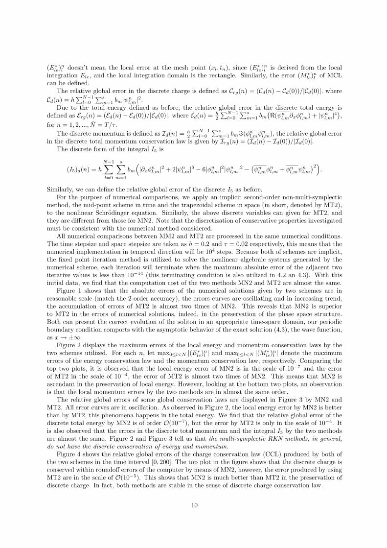
The relative global errors of some global conservation laws are displayed in Figure 3 by MN2 andMT2. All error curves are in oscillation. As observed in Figure 2, the local energy error by MN2 is betterthan by MT2, this phenomena happens in the total energy. We find that the relative global error of thediscrete total energy by MN2 is of order O(10−7), but the error by MT2 is only in the scale of 10−4. Itis also observed that the errors in the discrete total momentum and the integral I5 by the two methodsare almost the same. Figure 2 and Figure 3 tell us that the multi-symplectic RKN methods, in general,do not have the discrete conservation of energy and momentum.

Figure 4 shows the relative global errors of the charge conservation law (CCL) produced by both ofthe two schemes in the time interval [0, 200]. The top plot in the figure shows that the discrete charge isconserved within roundoff errors of the computer by means of MN2, however, the error produced by usingMT2 are in the scale of O(10−5). This shows that MN2 is much better than MT2 in the preservation ofdiscrete charge. In fact, both methods are stable in the sense of discrete charge conservation law.

10

0 20 40 60 80 100 120 140 160 180 2000

0.05

0.1

0.15

0.2

0.25

0.3

0.35

0.4

time0 20 40 60 80 100 120 140 160 180 200

0

0.1

0.2

0.3

0.4

0.5

0.6

0.7

time

Figure 1: The error of numerical solutions of ψ(x, t) by MN2 (left) and by MT2 (right) respectively.

4.2 Experiment B

In the previous subsection, the symplectic Nystrom method applied to the space is only of second order.In this subsection we implement a numerical experiment, which has been studied in [14] elaborately,by two 3-stage 4-order Nystrom schemes, one is symplectic and the other is non-symplectic for givinga comparison as that given between MN2 and MT2 in Experiment A. In [14], the initial condition isψ(x, 0) = a(1 − 0.1 cos x) + b sinx, where a = 0.5 and b = 0 or 10−8; b = 10−8 means that a tinyasymmetry is introduced to the initial condition, as the author pointed out, the asymmetry is a littlemore subtle to deal with in the investigation. Here, in our numerical experiment, the spatial intervalis taken as [0, L], where L = 4π, and we choose N as the number of the spatial grid points, that is,the spatial stepsize is determined by h = L/N . In [14] three cases N = 32, N = 64 and N = 128are considered for not only symmetric and asymmetric initial data, and the method utilized in [14] isthat the LF2 scheme (namely, the mid-point scheme in this paper) is applied to the temporal and thepseudo-spectral method to the spatial. Here we consider the case N = 32 and b = 10−8, and the initialdata for ψ(x, t) is taken ψ(x, 0) = a(1 − 0.1 cos x) + b sinx, the same one as in [14]; for the initial dataof φ(x, t), we adopt φ(x, 0) = d

dxψ(x, 0) = 0.1a sin(x) + b cos(x). And we apply the implicit mid-pointscheme to the temporal direction and the temporal stepsize we take is τ = 0.015. In this experiment, wealso implement the following periodic conditions

ψ|0 = ψ|L, φ|0 = φ|L (4.5)

and the time interval [0, 900] (6× 104 time steps).We construct the symplectic and non-symplectic 3-stage 4-order Nystrom schemes, which can be

formulated as the following Butcher’s tabulars

0 −1/4 1/4 01/2 7/48 −1/48 01 1/6 1/3 0

1/6 1/3 01/6 2/3 1/6

and

0 0 0 01/2 17/96 −1/6 11/961 1/24 2/3 −5/24

1/6 1/3 01/6 2/3 1/6

respectively. We denote the multisymplectic RKN method, i.e., the implicit mid-point scheme appliedto the temporal and the 3-stage 4-order symplectic Nestrom scheme to the spatial, by MS-MN3 in

11

0 20 40 60 80 100 120 140 160 180 2002.44

2.46

2.48

2.5

2.52

2.54

2.56

2.58x 10

−7

time0 20 40 60 80 100 120 140 160 180 200

2.3

2.4

2.5

2.6

2.7

2.8

2.9

3x 10

−4

time

0 20 40 60 80 100 120 140 160 180 2006

6.5

7

7.5

8

8.5

9x 10

−4

time0 20 40 60 80 100 120 140 160 180 200

1.1

1.2

1.3

1.4

1.5

1.6

1.7

1.8x 10

−3

time

Figure 2: The maximum errors of the discrete local conservation laws, ECL(top), MCL(bottom),MN2(left) and MT2(right).

short. Simultaneously, the non-multisymplectic one is denoted by nMS-MN3. All numerical comparisonsbetween MS-MN3 and nMS-MN3 are processed under the same numerical conditions, and the iterationmethod for solving the the nonlinear algebraic system and the stop criteria of the iteration are the same asintroduced in Experiment A. Figs.5-8 are given by means of the two methods, MS-MN3 and nMS-MN3.

Figure 5 shows the maximum errors of the discrete local energy and momentum conservation lawsby the two methods in the time interval [0, 900]. All the errors displayed in this figure are in the samescale of O(10−2). Compared with the ones showed in Figure 2, it seems that the higher-order schemespreserve the local invariants are not as good as the lower-order ones, and we will see the same phenomenadisplayed in Figure 6, the contrary result we can see in Figure 7. And, the same point between Figure5 and Figure 2 is that, the errors are oscillating near 0 even after the so long computations, thus thehigh-order schemes are stable with respect to the local conservation laws numerically.

Figure 6 shows the global errors of the two total invariants, the discrete total energy and the integralI5. As shown in Figure 5, all the errors in this figure are of order O(10−2) and it doesn’t produce any driftin the long computation and this guarantee the numerical stability with respect to the two conservationlaws, the total energy and I5.

The global errors of the discrete total momentum obtained by MS-MN3 and nMS-MN3 are displayedin Figure 7. It exhibits some interesting phenomena of the evolutions of the errors here, the error by MS-MN3 is in the scale of O(10−7), and it is two orders of magnitude better than the other one. Moreover,the error by the multisymplectic method doesn’t have any growth, it is in the reasonable oscillation, butthe error by non-multisymplectic one has a linear growth.

Figure 8 exhibits the global errors in the discrete charge conservation law by the two method. Ob-serving in the two plots, it can be found that the remarkable advantage of the multi-symplectic RKNmethods is the precise preservation of discrete charge conservation law. In the top plot, it shows thatthe involution of the global error of the discrete conservation law is conserved in the scale of O(10−12),almost the roundoff error of the computer; compare with the top plot in Figure 4, there is a very small

12

error but normal accumulation in such long numerical computation. As for nMS-MN3, the error is onlyof order O(10−6), and it is an interesting phenomenon that the shape of this error is similar to that inthe discrete total momentum obtained by MS-MN3, i.e. the first plot in Figure 7.

4.3 Experiment C

In order to investigate the collision of solitons, we consider the following form of the nonlinear Schrodingerequation (4.1)

iψt + ψxx + 2|ψ|2ψ = 0. (4.6)

As discussed in (2.1)-(2.3), the above equation can be written as the following form

M∂tz + K∂xz = ∇zS(z), (4.7)

where z is the state vector variable as introduced in §2, M = M , K = −K and S(z) = − 12

((q2 + p2)2 +

v2 + w2). The initial condition on two-soliton interaction is given as follows

ψ|t=0 =1√2

[sech

( x√2

)exp

(ix

2

)+ sech

(12(x− 25)

)exp

(i0.12

x)]

. (4.8)

In this experiment, we apply a high-order scheme, i.e. 3-stage 6-order Gauss-Legendre RK method,to the temporal direction and the symplectic 2-stage 2-order Nestrom method introduced in ExperimentA to the spatial direction, we denote this method by GL3-N2 in short. In the sequel, we make use ofGL3-N2 to exhibit the two-solition interaction, and the space mesh-length h = 0.2 and the time mesh-length τ = 0.01. The computation time interval we choose here is [0, 100]. The spatial interval is takenas [−60, 120].

Figure 9 shows the real part and imaginary part of numerical result of the two-soliton interactionrespectively. The numerical solution depicts two waves where the shape evolution both before and aftercollision do not change obviously. The figure displays the correct behavior of the two-soliton interaction,and implies the good preservation of the phase space structure.

Figure 10 shows the maximum errors of local conservation laws by GL3-N2 in the time interval [0, 100].The error of the discrete local energy conservation law displayed in this figure is in the same scale ofO(10−13). However for the local momentum conservation law, the error is of O(10−2). Numerical resultsare very interesting! From the observing, one can find that the errors get to the maximums at a certaintime between 20 and 30, namely at the collision time of two waves.

The global errors of the discrete charge and the discrete total energy are exhibited in Figure 11. Theerror in charge is of order O(10−14), it matches the theoretical analysis in §3 very well. The error inenergy arrives at the scale of O(10−15), it is out of our expectation. And it gets to a local maximum,which look likes a local shock, at the collision time, the shock reflects the collision effect.

Figure 12 shows the global errors of the discrete total momentum and the integral I5. The globalerror of the momentum is in the scale of O(10−3) and the error of I5 is only of O(10−1), but both ofthem reach the maximums at the collision time, and this reflects the collision mechanism at some degreenumerically.

Generally speaking, the multi-symplectic RKN methods may not preserve the discrete total energy,the discrete total momentum and the integral I5 exactly. In our numerical experiment, the evolutions ofthe errors of the local momentum, the integral I5 and the total momentum have a similar character, thatis, before and after the collision time, the errors vary much more slowly with oscillation.

5 Conclusions

The concatenation of symplectic Runge-Kutta methods in temporal direction and symplectic Nystrommethods in spatial direction for nonlinear Schrodinger equations leads to the multi-symplectic integrators(so called multi-symplectic RKN methods). The conclusions of this paper are listed as follows.

13

• It is shown theoretically that the discrete total symplecticity (3.3) in temporal direction is preservedprecisely by the multi-symplectic RKN methods for nonlinear Schrodinger equations. Numericalresults reveal the stability of multi-symplectic RKN methods in the sense of classical conservationlaws and the good preservation of phase space structure.

• Theoretical and numerical results show that the remarkable advantage of multi-symplectic RKNmethods is the precise preservation of discrete (local and global) charge conservation law for theequations.

• Numerical implementation shows that multi-symplectic methods, in general, do not preserve energyconservation law, the multi-symplectic RKN methods are superior to non-multi-symplectic methodsin the energy conservation for nonlinear Schrodinger equations. An interesting observation is thatthe numerical accuracy of global energy under the multi-symplectic RKN discretization may reacha higher order in contrast to the accuracy of numerical solutions.

• Multi-symplectic RKN schemes of higher order in spatial and temporal directions are implementedin numerical experiments. The two-soliton interaction can be depicted correctly by means of multi-symplectic RKN methods. Some interesting numerical results are exhibited, and they reveal thesuperiorities of multi-symplectic RKN methods not only in the conservation of multi-symplecticgeometric structure, but also in the preservation of some crucial conservative properties in physics.

AcknowledgementThe authors are grateful to the referees for their helpful comments and important suggestions.

References

[1] T.J. Bridges, Muti-symplectic structures and wave propagation, Math. Proc. Camb. Phil. Soc. 121(1997), 147-190.

[2] T. J. Bridges and S. Reich, Multi-symplectic integrators: numerical schemes for Hamiltonian PDEsthat conserve sysmplecticity, Phys. Lett. A 284 (2001) 184-193.

[3] Q. Chang, E. Jia, and W. Sun, Difference schemes for solving the generalized nonlinear Schrodingerequation, J. Comput. Phys. 148 (1999) 397-415.

[4] E. Hairer, C. Lubich and G. Wanner, Geometric Numerical Integration, Springer-Verlag BerlinHeidelberg, 2002.

[5] J. Hong and Y. Liu, A novel numerical approach to simulating nonlinear Schrodinger equation withvarying coefficients, Appl. Math. Lett. 16 (2003) 759-765.

[6] J. Hong, Y. Liu, Hans Munthe-Kaas and Antonella Zanna, Globally conservative properties anderror estimation of a multi-symplectic scheme for Schrodinger equations with variable coefficients,Appl. Numer. Math. 56 (2006) 814-843.

[7] J. Hong, H. Liu and G. Sun,The Multi-symplecticity of partitioned Runge-Kutta methods for Hamil-tonian PDEs, Math. Comp. 75 (2006) 167-181.

[8] J. Hong, C. Li, Multi-symplectic Runge-Kutta methods for nonlinear Dirac equations, J. Comput.Phys. 211 (2006) 448-472.

[9] A. Iserles, A First Course in the Numerical Analysis of Differential Equations, Cambridge UniversityPress, Cambridge 1996.

[10] A. L. Islas, D. A. Karpeev and C. M. Schober, Geometric integrators for the nonlinear Schrodingerequation, J. Comput. Phys. 173 (2001) 116-148.

14

[11] A. L. Islas and C. M. Schober, On the preservation of phase space structure under multisymplecticdiscretization, J. Comput. Phys. 197 (2004) 585-609.

[12] B. Leimkuhler and S. Reich, Simulating Hamiltonian Dynamics, Cambridge Monographs on Appliedand Computational Mathematics 14, Cambridge University Press, Cambredge 2004

[13] J. E. Marsden, S. Pekarsky, S. Shkoller and M. West, Variational methods, multisymplectic geometryand continuum mechanics, J. Geom. and Phys. 38 (2001) 253-284.

[14] R. McLachlan, Symplectic integration of Hamiltonian wave equations, Numer. Math. 66 (1994)465-492.

[15] B. Moore, S. Reich, Multisymplectic integration methods for Hamiltonian PDEs, Future Gener.Comput. Syst. 19 (2003) 395-402.

[16] B. Moore and S. Reich, Backward error analysis for multi-symplectic integration methods. Numer.Math. 95 (2003) 625-652.

[17] S. Reich, Multi-symplectic Runge-Kutta collocation methods for Hamiltonian wave equation, J.Comput. Phys. 157 (2000), 473-499.

[18] J. M. Sanz-Serna and M. P. Calvo, Numerical Hamiltonian Problems, Chapman & Hall, London1994.

[19] Y. B. Suris, On the conservation of the symplectic structure in the numerical solution of Hamiltoniansystems (in Russian), In: Numerical Solution of Ordinary Differential Equations, ed. S. S. Filippov,Keldysh Institute of Applied Mathematics, USSR Academy of Sciences, Moscow, 1988, 148-160.

[20] Y. B. Suris, The canonicity of mapping generated by Runge-Kutta type methods when integratingthe systems x = −∂U/∂x, Zh. Vychisl. Mat. i Mat. Fiz. 29 (1989) 138-144.

15

0 20 40 60 80 100 120 140 160 180 2000

0.5

1

1.5

2

2.5

3

3.5

4x 10

−7

time

0 20 40 60 80 100 120 140 160 180 200

−8

−6

−4

−2

0

x 10−4

time

0 20 40 60 80 100 120 140 160 180 200−7

−6

−5

−4

−3

−2

−1

0x 10

−5

time0 20 40 60 80 100 120 140 160 180 200

0

0.5

1

1.5

2

2.5

3x 10

−4

time

0 20 40 60 80 100 120 140 160 180 2000

0.5

1

1.5

2

2.5

3

3.5x 10

−3

time0 20 40 60 80 100 120 140 160 180 200

−6

−5

−4

−3

−2

−1

0x 10

−3

time

Figure 3: The relative global errors of the total conservation laws, the discrete total energy(top), thediscrete total momentum(middle) and the discrete conserved integral I5(bottom). The left figures areobtained by using MN2 and the right ones by MT2.

16

0 20 40 60 80 100 120 140 160 180 200−2

−1.5

−1

−0.5

0

0.5

1x 10

−12

time

0 20 40 60 80 100 120 140 160 180 2000

0.5

1

1.5

2

2.5

3

3.5

4

4.5x 10

−5

time

Figure 4: The relative global error of the discrete charge, MN2(top), MT2(bottom).

0 100 200 300 400 500 600 700 800 900−0.01

0

0.01

0.02

0.03

0.04

0.05

time0 100 200 300 400 500 600 700 800 900

−0.01

0

0.01

0.02

0.03

0.04

0.05

0.06

0.07

0.08

time

0 100 200 300 400 500 600 700 800 9000

0.005

0.01

0.015

time0 100 200 300 400 500 600 700 800 900

−0.01

0

0.01

0.02

0.03

0.04

0.05

0.06

0.07

0.08

time

Figure 5: The maximum errors of the discrete local conservation laws. Top: ECL; bottom: MCL. Theleft is obtained by using MS-MN3 and the right by nMS-MN3.

17

0 100 200 300 400 500 600 700 800 900−0.025

−0.02

−0.015

−0.01

−0.005

0

0.005

0.01

time0 100 200 300 400 500 600 700 800 900

−20

−15

−10

−5

0

5x 10

−3

time

0 100 200 300 400 500 600 700 800 900−0.045

−0.04

−0.035

−0.03

−0.025

−0.02

−0.015

−0.01

−0.005

0

time0 100 200 300 400 500 600 700 800 900

−0.045

−0.04

−0.035

−0.03

−0.025

−0.02

−0.015

−0.01

−0.005

0

time

Figure 6: The global errors of the discrete energy and I5. Top: the discrete total energy; bottom: I5.MS-MN3(left) and nMS-MN3(right).

0 100 200 300 400 500 600 700 800 900−8

−6

−4

−2

0

2

4

6

8x 10

−7

time0 100 200 300 400 500 600 700 800 900

−5

0

5

10

15

20x 10

−6

time

Figure 7: The global errors of the discrete total momentum, MS-MN3 (left) and nMS-MN3(right).

18

0 100 200 300 400 500 600 700 800 900−3

−2.5

−2

−1.5

−1

−0.5

0

0.5

1x 10

−12

time

0 100 200 300 400 500 600 700 800 900−2

−1.5

−1

−0.5

0

0.5

1x 10

−6

time

Figure 8: The global errors of the discrete charge, the top shows that by MS-MN3 and the bottom bynMS-MN3.

Figure 9: The numerical solutions of ψ(x, t) by GL3-N2, the left one is the real part q(x, t) and the rightis the imaginary part p(x, t).

19

0 10 20 30 40 50 60 70 80 90 1000

0.5

1

1.5

2

2.5

3

3.5x 10

−13

time0 10 20 30 40 50 60 70 80 90 100

0

0.01

0.02

0.03

0.04

0.05

0.06

0.07

0.08

0.09

0.1

time

Figure 10: The maximum errors of the local discrete energy (left) and momentum (right) conservationlaws.

0 10 20 30 40 50 60 70 80 90 100−1

0

1

2

3x 10

−14

time0 10 20 30 40 50 60 70 80 90 100

−1

−0.5

0

0.5

1

1.5

2

2.5

3

3.5x 10

−15

time

Figure 11: The global errors of the discrete charge and the discrete total energy.

0 10 20 30 40 50 60 70 80 90 100−1

0

1

2

3

4

5x 10

−3

time0 10 20 30 40 50 60 70 80 90 100

0

0.1

0.2

0.3

0.4

0.5

0.6

0.7

time

Figure 12: The global errors of the discrete conservation laws, the discrete momentum (top) and thediscrete conserved integral I5 (bottom).

20