Embed Size (px)
Citation preview

Multi-Stage Stochastic Programming with CVaR:Modeling, Algorithms and Robustness
Vaclav Kozmık
Faculty of Mathematics and PhysicsCharles University in Prague
December 11, 2014

Outline
Introduction Outline Original results
Structure of risk-averse multistage stochastic models Studied less than the risk-neutral case Risk measures bring multiple modeling possibilities
Nested models Multiperiod risk measures Sum of stage risks
Stochastic Dual Dynamic Programming Algorithm Originated in 1991 by Pereira & Pinto Well-studied for risk-neutral case Cut generation in risk-averse case is straightforward Upper bound estimation is challenging in risk-averse case
Outline
Variance reductions schemes Monte Carlo methods are widely applied, but they usually bring high
variance Many variance reduction schemes have been proposed: importance
sampling, stratified sampling, Quasi Monte Carlo, etc. Application of such schemes could be hard in practice, the proposals
usually focus on the method and toy examples, not on large-scale realworld applications
Contamination technique for multistage problems Captures various changes in the probability distribution First results applied to two-stage setups In multistage case, contamination was studied and applied for smaller
problems Extension to large-scale setups requires advanced algorithms
and techniques

Original results
New estimator for the policy value under the nested model setupwith CVaR Provides better results than the state-of-the-art estimators Can be used to build valid stopping rules for the SDDP algorithm General importance sampling scheme for mean-CVaR objectives
Closed-form solution provided for normal distribution Sampling algorithm presented for any general distribution to get the
suitable parameter of the variance reduction scheme
Contamination technique for large-scale multistage programs We provide an extension which accounts for the fact, that we can
never compute precise optimal solution Based on lower bounds from cutting-plane algorithms and upper
bounds from policy value estimators
Numerical study and comparison of two multi-stagemodels based on CVaR

Multistage stochastic optimization
Consider T stage stochastic program: Data process ξ = (ξ1, ξ2, . . . , ξT ) Decision process x = (x1, . . . , xT ) Stages should reflect the timing of decisions, steps can be unequal Filtration Ft generated by the projection Πtξ = ξ[t] := (ξ1, . . . , ξt) Probability distribution of ξ: P Pt denotes the marginal probability distribution of ξt Pt
[·|ξ[t−1]
]denotes the conditional probability distribution
The decision process is nonanticipative: Decisions taken at any stage of the process do neither depend on
future realizations of stochastic data nor on future decisions xt is Ft-measurable The sequence of decisions and observations is:
x1, ξ2, x2(x1, ξ2), . . . , xT (xT−1, ξ2, . . . , ξT )
its random outcome f (x, ξ)
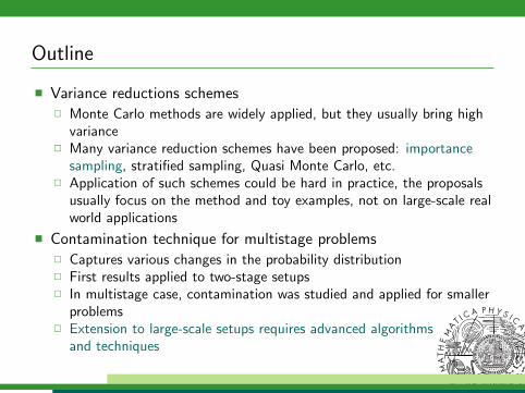
Scenario tree
stage 1 stage 2 stage 3 stage 4
x1
ξ1
x2(x1, ξ12)
ξ12
x2(x1, ξ22)
ξ22
x3(x2, ξ12, ξ
13)
ξ13
x3(x2, ξ12, ξ
23)
ξ23
x3(x2, ξ22, ξ
33)
ξ33
x3(x2, ξ22, ξ
43)
ξ43

Multistage stochastic optimization
Nested form of multistage stochastic linear program (MSLP):
minx1∈X1
c>1 x1 + EP [Q2(x1, ξ2)] with X1 := x1|A1x1 = b1, x1 ≥ 0
With Qt(xt−1, ξ[t]), t = 2, . . . ,T , defined recursively as
Qt(xt−1, ξ[t]) = minxt
ct(ξ[t])>xt + EPt+1[·|ξ[t]]
[Qt+1(xt , ξ[t+1])
] Xt(xt−1, ξ[t]): At(ξ[t−1])xt = bt(ξ[t−1])− Bt(ξ[t−1])xt−1, xt ≥ 0 a.s.,
In the case of stagewise independence the conditional distributionsboil down to marginal distributions Pt of ξt
We assume: Constraints involving random elements hold almost surely All optimal solutions exist, which is related with the
relatively complete recourse All conditional expectations exist
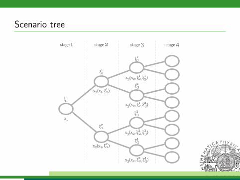
Risk-averse multistage programs
In the risk-neutral programs possible risks are not reflected
Risk measure is a functional which assigns a real value to therandom outcome f (x, ξ)
Risk measures depend on decisions and probability distribution P. Filtration F1 ⊂ · · · ⊂ Ft · · · ⊆ F should be taken into account
Risk monitoring in individual stages should be incorporated
minx1
c>1 x1+ρ2
(minx2
c2(ξ[1])>x2 + · · ·+ ρT
(minxT
cT (ξ[T−1])>xT
))
Different risk measures ρt can be applied in each stage
Coherence of ρ is mostly expected [Artzner et al., 2007]

Time consistency
Many different definitions
Need to distinguish between time consistency of the risk measureand time consistency of the model
TC1 [Carpentier, et al., 2012] The sequence of dynamicoptimization problems is dynamically consistent if the optimalstrategies obtained when solving the original problem remainoptimal for all subsequent problems.
TC2 [Shapiro, 2009] At each state of the system, optimality of adecision policy should not involve states which cannot happen inthe future.
Risk-neutral stochastic programs are time consistent
In general, time consistency for risk-averse stochastic programsdoes not hold true

Nested CVaR risk measure
Consider sequence of random costs Z = (Z1, . . . ,ZT )
Nested CVaR risk measure is given by:
ρn (Z) = CVaRα [·|F1] · · · CVaRα [·|FT−1]
(T∑t=1
Zt
)
The interpretation is not straightforward can be viewed as the cost we would be willing to pay at the first stage
instead of incurring the sequence of random costs Z1, . . . ,ZT
cf. Ruszczynski [2010]

Nested CVaR model
Risk measures are usually combined with expectation to getefficient solutions
Given risk coefficients λt and random loss variable Z we define:
ρt,ξ[t−1][Z ] = (1− λt)E
[Z |ξ[t−1]
]+ λt CVaRαt
[Z |ξ[t−1]
] Nested model can be written:
minA1x1=b1,x1≥0
c>1 x1 + ρ2,ξ[1]
[min
B2x1+A2x2=b2,x2≥0c>2 x2 + · · ·
· · ·+ ρT ,ξ[T−1]
[min
BT xT−1+AT xT =bT ,xT≥0c>TxT
]] Time consistent w.r.t. [TC1] and [TC2]

Nested CVaR model
Allows to develop dynamic programming equations, using:
CVaRα [Z ] = minu
[u +
1
αE [Z − u]+
] Denote Qt(xt−1, ξ[t]), t = 2, . . . ,T as the optimal value of:
Qt(xt−1, ξ[t]) = minxt ,ut
c>t xt + λt+1ut +Qt+1(xt , ut , ξ[t])
s.t. Atxt = bt − Btxt−1
xt ≥ 0,
Recourse function Qt+1(xt , ut , ξ[t]) is given by (QT+1(·) ≡ 0):
EPt+1[·|ξ[t]]
[(1− λt+1) Qt+1(xt , ξ[t+1]) +
λt+1
αt+1
[Qt+1(xt , ξ[t+1])− ut
]+
].

Multiperiod CVaR risk measure
Based on the following risk measure:
ρm (Z) =T∑t=2
µtE [CVaRαt [Zt |Ft−1]] .
The difference between this risk measure and the nested CVaR riskmeasure is that here we apply expectation instead of the nesting
Easier interpretation Averaging of the risks in future stages
Polyhedral risk measure Solution of a multi-stage stochastic linear program of a special form Optimization of the original problem can be combined with
the optimization problem which defines the risk measure

Multiperiod CVaR model
Stochastic programming model:
minx1,...,xT
c>1 x1 + µ2E[ρ2,ξ[1]
[c>2 x2
]]+ · · ·+ µTE
[ρT ,ξ[T−1]
[c>TxT
]]s.t. A1x1 = b1
A2x2 = b2 − B2x1
...
ATxT = bT − BTxT−1
xt ≥ 0, xt ∈ Lp (Ω,Ft ,P) t = 1, . . . ,T .
Time consistent w.r.t. [TC1] and [TC2]
Dynamic programming equations are developed,similarly to the nested case

Sum of CVaR model
The weighted sum of CVaR model is based on the following riskmeasure:
ρs (Z) =T∑t=2
µt CVaRαt [Zt ]
with∑T
t=2 µt = 1, µt ≥ 0 ∀t. No nesting or averaging is present Easy interpretation - weighted sum of CVaR for all stages Related to multi-criteria optimization
“We want to hedge against risk in all stages separately”
Dynamic programming equations show that all ut are decided inthe first stage
Corresponding model is time consistent w.r.t. [TC1],but not w.r.t. [TC2]

Asset allocation model
At stage t we observe the price ratio between the new price andthe old price rt
xt contains the optimal allocation (in USD, say)
The total portfolio value is tracked as a multiple of the initial value
Dynamic programming equations are very simple:
minxt ,ut
− 1>xt + λt+1ut +Qt+1(xt , ut)
s.t. r>t xt−1 − 1>xt = 0
xt ≥ 0
Transaction costs of ft1>|xt − xt−1| can be included
We solve problems up to 15 stages with 1024 scenarios,using SDDP with importance sampling
SDDP algorithm
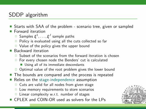
Starts with SAA of the problem - scenario tree, given or sampled Forward iteration
Samples ξ1, . . . , ξJ sample paths Policy is evaluated using all the cuts collected so far Value of the policy gives the upper bound
Backward iteration Subset of the scenarios from the forward iteration is chosen For every chosen node the Benders’ cut is calculated
Using all of its immediate descendants Optimal value of the root problem gives the lower bound
The bounds are compared and the process is repeated Relies on the stage-independence assumption
Cuts are valid for all nodes from given stage Low memory requirements to store scenarios Linear complexity w.r.t. number of stages
CPLEX and COIN-OR used as solvers for the LPs

Upper bound overview
Risk-neutral problems The value of the current optimal policy can be estimated easily Expectation at each node can be estimated by single chosen
descendant Risk-averse problems
To estimate the CVaR value we need more descendants in practice Leads to intractable estimators with exponential computational
complexity, denoted by Ue
Current solution (to our knowledge) Run the risk-neutral version of the same problem and determine the
number of iterations needed to stop the algorithm, then run the samenumber of iterations on the risk-averse problem
Inner approximation scheme proposed by Philpott et al. [2013] Works with different policy than the outer approximation Probably the best alternative so far Does not scale well with the dimension of x

Upper bound enhancements
State-of-the-art estimator runs with exponential complexity We need an estimator with linear complexity to build valid bounds Ideally it should be unbiased, or in practice, have small bias We start with the linear estimator from the risk-neutral case
and include: Importance sampling, with an additional assumption needed Further enhancements to reduce bias and volatility
Assumption
Let at(xt−1, ξt) approximate the recourse value of our decisions xt−1
after the random parameters ξt have been observed, and letat(xt−1, ξt) be cheap to evaluate.
For example in our portfolio model:at(xt−1, ξt) = −ξ>t xt−1 = −r>t xt−1
Importance sampling
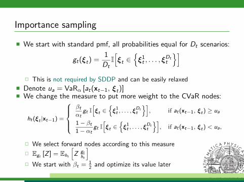
We start with standard pmf, all probabilities equal for Dt scenarios:
gt(ξt) =1
DtI[ξt ∈
ξ1t , . . . , ξ
Dtt
] This is not required by SDDP and can be easily relaxed
Denote ua = VaRα [at(xt−1, ξt)] We change the measure to put more weight to the CVaR nodes:
ht(ξt |xt−1) =
βtαt
gt I[ξt ∈
ξ1t , . . . , ξ
Dtt
], if at(xt−1, ξt) ≥ ua
1− βt1− αt
gt I[ξt ∈
ξ1t , . . . , ξ
Dtt
], if at(xt−1, ξt) < ua,
We select forward nodes according to this measure
Egt [Z ] = Eht
[Z gt
ht
] We start with βt = 1
2 and optimize its value later

Linear estimators
The nodes can be selected randomly from the standard i.i.d.measure or from the importance sampling measure
For stages t = 2, . . . ,T is given by:
vt(ξjt−1
t−1) = (1− λt)(
(cjtt )>xjtt + vt+1(ξjtt ))
+
+ λtujt−1
t−1 +λtαt
[(cjtt )>xjtt + vt+1(ξjtt )− u
jt−1
t−1
]+
vT+1(ξjTT ) ≡ 0
Along a single path for scenario j the cost is estimated by:
v(ξj) = c>1 x1 + v2
Linear estimators
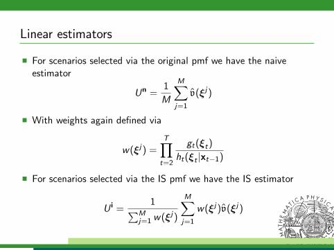
For scenarios selected via the original pmf we have the naiveestimator
Un =1
M
M∑j=1
v(ξj)
With weights again defined via
w(ξj) =T∏t=2
gt(ξt)
ht(ξt |xt−1)
For scenarios selected via the IS pmf we have the IS estimator
U i =1∑M
j=1 w(ξj)
M∑j=1
w(ξj)v(ξj)

Linear estimators - validity
Function U i provides an asymptotic upper bound estimator for theSAA version of the presented optimization problem.
Proposition
Assume finite optimal value, relatively complete recourse andinterstage independence. Let ϕ denote the optimal value. Let ξdenote a sample path selected under the empirical distribution, andlet v(ξ) be defined for that sample path. Then Eg [v(ξ)] ≥ ϕ.Furthermore if ξj , j = 1, . . . ,M, are i.i.d. and generated by the ISpmfs then U i → Eg [v(ξ)], w.p.1, as M →∞.

Upper bound enhancements
Linear estimator still degrades for problems with 10 or 15 stages The reason for the bias of the estimator comes from poor
estimates of CVaR Once the cost estimate for stage t exceeds ut−1 the difference is
multiplied by α−1t
When estimating stage t − 1 costs in the nested model we sum staget − 1 costs and stage t estimate which means that we usually end upwith costs greater than ut−2 so another multiplication occurs
This brings both bias and large variance
Assumption
For every stage t = 2, . . . ,T and decision xt−1 the approximationfunction at satisfies:
Qt ≥ VaRαt [Qt ] if and only if at ≥ VaRαt [at ] .
Improved estimator
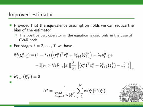
Provided that the equivalence assumption holds we can reduce thebias of the estimator The positive part operator in the equation is used only in the case of
CVaR node
For stages t = 2, . . . ,T we have
vat (ξjt−1
t−1) = (1− λt)(
(cjtt )>xjtt + vat+1(ξjtt ))
+ λtujt−1
t−1+
+ I[at > VaRαt [at ]]λtαt
[(cjtt )>xjtt + vat+1(ξjtt )− u
jt−1
t−1
]+
vaT+1(ξjTT ) ≡ 0
Ua =1∑M
j=1 w(ξj)
M∑j=1
w(ξj)va(ξj)

Improved estimator - validity
Function Ua provides an asymptotic upper bound estimator for theSAA version of the presented optimization problem.
Proposition
Assume finite optimal value, relatively complete recourse andinterstage independence. Let ϕ denote the optimal value Let ξ denotea sample path selected under the empirical distribution and let the“perfect ordering” assumption hold. Then Eg [va(ξ)] ≥ ϕ. If ξj ,j = 1, . . . ,M, are i.i.d. and generated by the IS pmfs thenUa → Eg [va(ξ)], w.p.1, as M →∞. Furthermore, if the subproblemsinduce the same policy for both v(ξ) and va(ξ) thenEg [v(ξ)] ≥ Eg [va(ξ)] .

Improved estimator results
Comparison with exponential estimator Ue from the literature:
T z Un (s.d.) U i (s.d.) Ua (s.d.) Ue (s.d.)
2 -0.9518 -0.9515 (0.0020) -0.9517 (0.0012) -0.9517 (0.0011) -0.9518 (0.0019)
3 -1.8674 -1.8300 (0.0145) -1.8285 (0.0108) -1.8656 (0.0060) -1.8013 (0.0302)
4 -2.7811 -2.4041 (0.1472) -2.3931 (0.1128) -2.7764 (0.0126) -2.6027 (0.0883)
5 -3.6794 -3.4608 (0.1031) -3.4963 (0.1008) -3.6731 (0.0303) -2.9031 (0.5207)
10 -7.6394 9.3× 10⁴ (1.4× 10⁴) 9.0× 10⁴ (8.7× 10⁴) -7.5465 (0.2562) 1.5× 10⁷ (1.3× 10⁶)
15 -11.5188 NA NA -11.0148 (0.6658) NA
For T = 2, . . . , 5 variance reduction of Ua relative to Ue:3 to 25 to 50 to 300.
Computation time for Un for T = 5, 10, 15:8.7 sec. to 31.6 sec. to 67.4 sec.
Computation time for Ua for T = 5, 10, 15:6.8 sec. to 30.0 sec. to 66.5 sec.
Can be extended to handle more complex models, forinstance asset allocation with transaction costs

Variance reduction
We consider a functional from our model:
Qα [Z ] = (1− λ)E [Z ] + λCVaRα [Z ]
We define:
Qs = (1− λ) Z + λ
(uZ +
1
α[Z − uZ ]+
)Q i =
g
h
((1− λ) Z + λ
(uZ +
1
α[Z − uZ ]+
)) It clearly holds Q = Eh
[Q i]
= Eg [Qs ]
Our aim is to find suitable parameter β for our importancesampling scheme, so that varh
[Q i]< varg [Qs ]

Example - normal distribution
beta
N(0,1)N(1,1)N(1,0.5)N(-1,1)
0.2 0.4 0.6 0.8 1.0
0.10
0.15
0.20
0.25
0.30
lambda

Other distributions
We can also estimate the suitable β by sampling We choose a mesh of possible values, e.g. B = 0.01, 0.02, . . . , 0.99 For each of them, we sample prescribed number of scenarios, Z j
We compute the mean and variance of the values Q j given by Z j
The lowest variance is selected as a suitable choice of β
Even though we start with log-normal distribution, convolution andnested structure of our model brings complex transformations
Different values of β should be selected for every stage, as theparameters of the distributions also vary
We have values β estimated by the algorithm for generaldistributions on 100, 000 scenarios
An alternative would be β = 0.3 which provideslow variance for most of our charts
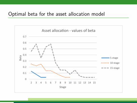
Optimal beta for the asset allocation model
0
0.1
0.2
0.3
0.4
0.5
0.6
0.7
2 3 4 5 6 7 8 9 10 11 12 13 14 15
Beta
Stage
Asset allocation - values of beta
5-stage
10-stage
15-stage

Results
Standard Monte Carlo setup Qs (βt = αt = 0.05)
Improved estimator Qi with variable βt based on our analysis
Lower bound z
T total scenarios z Qs (s.d.) Qi (s.d.)
5 6, 250, 000 -3.5212 -3.5166 (0.0168) -3.5170 (0.0111)
10 ≈ 1015 -7.3885 -7.2833 (0.2120) -7.2838 (0.0303)
15 ≈ 1024 -10.4060 -10.1482 (0.8184) -10.1245 (0.1355)
For T = 5, 10, 15 we achieved roughly 35%, 85% and 85%reduction of standard deviation
Negligible effect on computation times

Contamination for multistage risk-averse problems
Captures various changes in the probability distribution Assume that it’s possible to reformulate the stochastic program as:
minx∈X
F (x,P) := minx∈X
∫Ω
f (x, ξ)P(dξ)
Simplest case of contamination, we obtain global bounds It’s possible to reformulate our CVaR model with auxiliary variable u
in this way Let Q be another fixed probability distribution and define
contaminated distributions
Pk := (1− k)P + kQ, k ∈ [0, 1]
Suppose that the stochastic program has a solutionϕ(k) := minx∈X F (x,Pk) for all these distributions

Contamination for multistage risk-averse problems
Suppose nonempty, bounded set of optimal solutions X ∗(P) of theinitial stochastic program
Then the directional derivative is given by:
ϕ′(0+) = minx∈X ∗(P)
F (x ,Q)− ϕ(0)
ϕ(k) concave on [0, 1]
The contamination bounds follow:
(1− k)ϕ(0) + kϕ(1) ≤ ϕ(k) ≤ ϕ(0) + kϕ′(0+), k ∈ [0, 1]
Contamination for multistage risk-averse problems
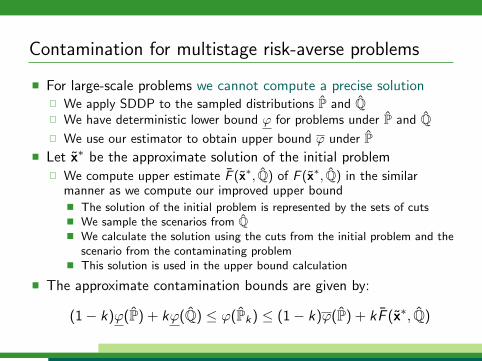
For large-scale problems we cannot compute a precise solution We apply SDDP to the sampled distributions P and Q We have deterministic lower bound ϕ for problems under P and Q We use our estimator to obtain upper bound ϕ under P
Let x∗ be the approximate solution of the initial problem We compute upper estimate F (x∗, Q) of F (x∗, Q) in the similar
manner as we compute our improved upper bound The solution of the initial problem is represented by the sets of cuts We sample the scenarios from Q We calculate the solution using the cuts from the initial problem and the
scenario from the contaminating problem This solution is used in the upper bound calculation
The approximate contamination bounds are given by:
(1− k)ϕ(P) + kϕ(Q) ≤ ϕ(Pk) ≤ (1− k)ϕ(P) + kF (x∗, Q)

Numerical results
Monthly data from Prague Stock Exchange, January 2009 toFebruary 2012
Risk aversion coefficients set to λt = 10%
Contaminating distribution Q was obtained by increasing thevariance by 20%
3 and 5 stage problems with 1, 000 descendants per node
We have calculated the derivative values for 10 times and usedtheir mean as well as empirical statistical upper bound

Results - 3 stages without transaction costs
-2.043
-2.042
-2.041
-2.040
-2.039
-2.038
-2.037
-2.036
0.00
0.05
0.10
0.15
0.20
0.25
0.30
0.35
0.40
0.45
0.50
0.55
0.60
0.65
0.70
0.75
0.80
0.85
0.90
0.95
1.00
Obj
ectiv
e fu
nctio
n
Contamination bounds for parameter k
upper b.
lower b.

Results - 5 stages without transaction costs
-4.15
-4.14
-4.13
-4.12
-4.11
-4.10
-4.09
-4.08
-4.07
-4.06
0.00
0.05
0.10
0.15
0.20
0.25
0.30
0.35
0.40
0.45
0.50
0.55
0.60
0.65
0.70
0.75
0.80
0.85
0.90
0.95
1.00
Obj
ectiv
e fu
nctio
n
Contamination bounds for parameter k
stat. upper b.
upper b. mean
lower b.

Model comparison
Monthly data from Prague Stock Exchange, January 2009 toFebruary 2012
asset mean std. deviationAAA 1.0290 0.1235
CETV 0.9984 0.2469
CEZ 0.9990 0.0647
ERSTE GROUP BANK 1.0172 0.1673
KOMERCNI BANKA 1.0110 0.1157
ORCO 1.0085 0.2200
PEGAS NONWOVENS 1.0221 0.0863
PHILIP MORRIS CR 1.0213 0.0719
TELEFONICA C.R. 0.9993 0.0595
UNIPETROL 1.0079 0.0843
VIENNA INSURANCE GROUP 1.0074 0.1100
Model comparison
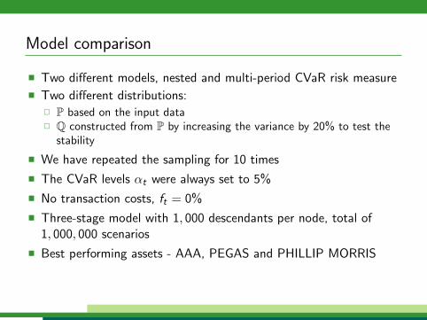
Two different models, nested and multi-period CVaR risk measure Two different distributions:
P based on the input data Q constructed from P by increasing the variance by 20% to test the
stability
We have repeated the sampling for 10 times
The CVaR levels αt were always set to 5%
No transaction costs, ft = 0%
Three-stage model with 1, 000 descendants per node, total of1, 000, 000 scenarios
Best performing assets - AAA, PEGAS and PHILLIP MORRIS

Model comparison
Both models relatively stable with respect to variance of theunderlying distribution
Nested model has more stable solutions and better diversification
When increasing λt , solutions become more stable in both models
λt model distr. AAA PEGAS PHILIP M.
0.1 nested P 0.2388 (0.1133) 0.3893 (0.1109) 0.3720 (0.1011)
0.1 nested Q 0.2718 (0.1600) 0.3582 (0.0902) 0.3700 (0.1565)
0.1 multiper. P 0.6034 (0.3681) 0.2262 (0.2084) 0.1704 (0.2000)
0.1 multiper. Q 0.6032 (0.3453) 0.1660 (0.1562) 0.2308 (0.2369)
0.2 nested P 0.1774 (0.0681) 0.4132 (0.0774) 0.4032 (0.0907)
0.2 nested Q 0.1730 (0.0541) 0.3471 (0.0566) 0.4545 (0.0429)
0.2 multiper. P 0.3081 (0.1472) 0.2993 (0.1757) 0.3926 (0.0990)
0.2 multiper. Q 0.3127 (0.1776) 0.3963 (0.0975) 0.2910 (0.1781)

Future research
Statistical properties of the proposed upper bound estimators
Approximation functions applicable in importance samplingschemes for various practical problems
Application in hydroelectric scheduling under inflow uncertainty Develop analogous schemes and estimators for other risk measures
Spectral risk measures based on CVaR
Scenario reduction techniques under stage-wise independence More general structures without the stage-wise independence
assumption Markov chains Additive dependence models
Implement parallel processing for SDDP

References
ARTZNER, P., DELBAEN, F., EBER, J.-M., HEATH, D. andKU, H. (2007): Coherent multiperiod risk adjusted values andBellman’s principle, Annals of Operations Research vol. 152, pp.2–22
CARPENTIER, P., CHANCELIER, J. P., COHEN, G., DELARA, M. and GIRARDEAU, P. (2012): Dynamic consistency forstochastic optimal control problems, Annals of OperationsResearch vol. 200, pp. 247–263
DUPACOVA, J. (1995): Postoptimality for multistage stochasticlinear programs, Ann. Oper. Res. vol. 56, pp. 65–78
PEREIRA, M. V. F. and PINTO, L. M. V. G. (1991): Multi-stagestochastic optimization applied to energy planning, MathematicalProgramming vol. 52, pp. 359–375.

References
PHILPOTT, A. B., DE MATOS, V. L., FINARDI, E. C. (2013):On Solving Multistage Stochastic Programs with Coherent RiskMeasures. Oper. Res. vol. 61, pp. 957–970
PHILPOTT, A. B. and GUAN, Z. (2008): On the convergence ofsampling-based methods for multi-stage stochastic linear programs,Operations Research Letters vol. 36, pp. 450–455.
ROCKAFELLAR, R. T. and URYASEV, S. (2002): Conditionalvalue at risk for general loss distributions, Journal of Banking &Finance vol. 26, pp. 1443–1471
RUSZCZYNSKI, A. (2010): Risk-averse dynamic programming forMarkov decision processes, Mathematical Programming, vol. 125,pp. 235–261.

References
RUSZCZYNSKI, A. and SHAPIRO, A. (2006): Conditional riskmappings, Mathematics of Operations Research vol. 31, pp.544–561.
SHAPIRO, A. (2011): Analysis of stochastic dual dynamicprogramming method, European Journal of Operational Research209, pp. 63-72.
SHAPIRO, A. (2009): On a time consistency concept in risk aversemultistage stochastic programming, Operations Research Lettersvol. 37, pp. 143–147

Publications
DUPACOVA, J. and KOZMIK, V. (2014): Stress Testing forRisk-Averse Stochastic Programs To appear in Acta Mathematica Universitatis Comenianae
KOZMIK, V. (2014): On Variance Reduction of Mean-CVaRMonte Carlo Estimators Accepted in Computational Management Science, doi:
10.1007/s10287-014-0225-7
DUPACOVA, J. and KOZMIK, V. (2014): Structure ofRisk-Averse Multistage Stochastic Programs Accepted in OR Spectrum, doi: 10.1007/s00291-014-0379-2
KOZMIK, V. and MORTON, D. (2014): Evaluating policies inrisk-averse multi-stage stochastic programming Accepted in Mathematical Programming Series A, doi:
10.1007/s10107-014-0787-8

Publications
KOZMIK, V. (2012): Multistage risk-averse asset allocation withtransaction costs, Proceedings of 30th International ConferenceMathematical Methods in Economics, pp. 455–460.
KOZMIK, V. and KOPA, M. (2011): Stability of Mean-RiskModels with Log-Normal Distribution of Returns, MathematicalMethods in Economics 2011 Proceedings, pp. 363–368
KOZMIK, V. (2010): Convergence of Approximate Solutions inMean-Risk Models, Proceedings of 47th EWGFM meeting pp.81–88

Citations
RUSZCZYNSKI, A. (2014): Dynamic risk-averse optimization,Safety, Reliability, Risk and Life-Cycle Performance of Structuresand Infrastructures, New York: CRC Press, ISBN 978-1138000865.
HOMEM-DE-MELLO, T. and BAYRAKSAN, G. (2014): MonteCarlo Sampling-Based Methods for Stochastic Optimization,Surveys in Operations Research and Management Science, vol. 19,pp. 56–85.
GUIGUES, V. (2014): Convergence analysis of sampling-baseddecomposition methods for risk-averse multi-stage stochasticconvex programs, Preprint
MACEIRA, M. E. P., et al. (2014): Application of CVaR RiskAversion Approach in the Expansion and Operation Planning andfor Setting the Spot Price in the Brazilian HydrothermalInterconnected System. In: Power Systems ComputationConference, Wroclav.

Citations
DUPACOVA, J. (2013): Ways and means with scenarios, Bulletinof the Czech Econometric Society, vol. 20, pp. 112–123.
RUSZCZYNSKI, A. (2013): Advances in Risk-Averse Optimization,Tutorials in Operations Research: Theory Driven by InfluentialApplication, Maryland: Informs, ISBN 978-0-9843378-4-2.
WERNER, A. S. , PICHLER, A., MIDTHUN, K. T., HELLEMO, L.and TOMASGARD, A. (2013): Risk Measures in Multi-HorizonScenario Trees, Handbook of Risk Management in EnergyProduction and Trading, New York: Springer, ISBN978-1461490340.
ZHANG, W. (2013): Water Network Design and Management viaStochastic Programming, PhD Thesis, The University of Arizona.