Multi-sensor Adaptive Control System for IoT-empowered

Multi-sensor Adaptive Control System for IoT-empoweredSmart Lighting with Oblivious Mobile Sensors∗

AREG KARAPETYAN,Masdar Institute, Khalifa University

SID CHI-KIN CHAU, Australian National University

KHALED ELBASSIONI,Masdar Institute, Khalifa University

SYAFIQ KAMARUL AZMAN,Masdar Institute, Khalifa University

MAJID KHONJI,Masdar Institute, Khalifa University

Internet-of-things (IoT) have created a new paradigm of integrated sensing and actuation systems for various

intelligent monitoring and controlling applications in smart homes and buildings. One viable application is

IoT-empowered smart lighting systems that utilize the interplay between smart light bulbs (equipped with

controllable LED devices and wireless connectivity) and mobile sensors (embedded in users’ wearable devices

such as smart watches, spectacles and gadgets) to provide automated illuminance control functions tailored to

users’ preferences (e.g., of brightness, color intensity and color temperature). Despite the usefulness of smart

lighting systems, practical deployment usually precludes the inclusion of sophisticated but costly location-

aware sensors that are capable of mapping out the details of a dynamic environment. Instead, cheap obliviousmobile sensors are often utilized, which are plagued with uncertainty in the locations of sensors and light bulbs.

The presence of oblivious mobile sensors impedes the design of effective smart lighting systems for uncertain

indoor environments with multiple sensors and multiple light bulbs under time-varying background light

sources. In this article, we shed light on the adaptive control algorithms of smart lighting systems based on

oblivious mobile sensors. We first formulate a general model capturing an oblivious multi-sensor illuminance

control problem, and a robust adaptive control framework agnostic to a dynamic surrounding environment

with unknown parameters. With this model, we devise efficient algorithms for an adaptive illuminance control

system that can minimize energy consumption of light bulbs and satisfy users’ preferences. Our algorithms

are then studied under extensive empirical evaluations in a proof-of-concept smart lighting testbed system

with programmable smart light bulbs and mobile light sensors in smartphones. Furthermore, we discuss the

potential improvements in hardware development and practical extensions for future work.

CCS Concepts: • Human-centered computing→ Ambient intelligence; Ubiquitous and mobile com-

puting; • Theory of computation → Stochastic control and optimization; Online learning algorithms; •Computing methodologies → Optimization algorithms; • Computer systems organization → Sen-

sors and actuators; •Mathematics of computing→ Simulated annealing; • Hardware→ Sensor devicesand platforms.

∗This is an extended version of a prior conference paper appeared in ACM BuildSys 2018 [9]. See Appendix for a list of

changes in this journal version as compared to the prior version.

Authors’ addresses: Areg Karapetyan, Masdar Institute, Khalifa University, Abu Dhabi, UAE, [email protected];

Sid Chi-Kin Chau, Australian National University, Canberra, Australia, [email protected]; Khaled Elbassioni, Masdar

Institute, Khalifa University, Abu Dhabi, UAE, [email protected]; Syafiq Kamarul Azman, Masdar Institute, Khalifa

University, Abu Dhabi, UAE, [email protected]; Majid Khonji, Masdar Institute, Khalifa University, Abu Dhabi,

UAE, [email protected].

Permission to make digital or hard copies of all or part of this work for personal or classroom use is granted without fee

provided that copies are not made or distributed for profit or commercial advantage and that copies bear this notice and the

full citation on the first page. Copyrights for components of this work owned by others than the author(s) must be honored.

Abstracting with credit is permitted. To copy otherwise, or republish, to post on servers or to redistribute to lists, requires

prior specific permission and/or a fee. Request permissions from [email protected].

© 2019 Copyright held by the owner/author(s). Publication rights licensed to ACM.

1550-4859/2019/0-ART00 $15.00

https://doi.org/000000.000000

ACM Trans. Sensor Netw., Vol. 0, No. 0, Article 00. Publication date: 2019.

https://doi.org/000000.000000

00:2 A. Karapetyan, S. Chau, K. Elbassioni, S. Azman, and M. Khonji

Additional Key Words and Phrases: Smart Lighting Control System, Oblivious Mobile Sensors, Internet-of-

Things, Illuminance Control Algorithm, Wearable Computing.

ACM Reference Format:

Areg Karapetyan, Sid Chi-Kin Chau, Khaled Elbassioni, Syafiq Kamarul Azman, and Majid Khonji. 2019.

Multi-sensor Adaptive Control System for IoT-empowered Smart Lighting with Oblivious Mobile Sensors∗.

ACM Trans. Sensor Netw. 0, 0, Article 00 ( 2019), 22 pages. https://doi.org/000000.000000

1 INTRODUCTIONThe popular trend of Internet-of-things (IoT) is bolstered by the increasing needs for ubiquitous

computational intelligence embedded in diverse facilities and infrastructures. A vivid example is

in the area of smart homes and buildings, whereby automated control and management systems,

using IoT frameworks, can regulate appliances and facilities for enhancing user comfort and energy

efficiency. In keeping with this trend, modern lighting systems are witnessing a departure from

conventional incandescent lighting to embrace the energy-efficient LED technology, which supports

a wider range of reconfigurable brightness levels and colors. These controllable LED devices are also

integrated with system-on-a-chip to provide local computation andwireless connectivity supporting

mainstream network protocols (e.g., WiFi, ZigBee), giving rise to a new class of IoT devices as

known as smart light bulbs, such as Philips Hue, LIFX. In future, the advances in OLED technology

enables smart light bulbs to support a more vibrant color spectrum in flexible form factors that can

be integrated with our environment seamlessly, such as being embedded in furniture, decorations

and sculptures, for supporting artistic interior designs and novel infotainment applications. Given

their increasing affordability and effectiveness in simulating natural light, smart light bulbs are

becoming an integral component of modern buildings and smart homes.

Meanwhile, an IoT device requires a close integration of sensing and controlling technologies

to support advanced applications in dynamic environments. In more sophisticated applications

of illuminance management, smart light bulbs will need to incorporate the sensing data from

various wearable/mobile devices, such as smartphones, smart watches, wristbands, smart clothes,

spectacles and gadgets. With the advances in sensing technology, there are light-weight, low-

powered and cost-effective mobile sensors that can be embedded in all forms of wearable devices.

Thus, the combination of smart light bulbs and mobile sensors can enable a broad spectrum of novel

interactive illuminance applications to support personalized preferences and dynamic environments

(e.g., a personalizable lighting system that synchronizes with events and activities).

Nevertheless, the novel illuminance management applications considering flexible configurability,

dynamic environments and heterogeneous users’ preferences present new challenges, rendering

the traditional user-operated approach ineffective [22, 23]. Therefore, IoT-empowered smart lightingsystems require a new kind of automated control algorithms that can adapt to dynamic surrounding

environments as well as cater for heterogeneous contexts and user preferences in real time. To

this end, it needs a tight interplay between wireless controllable smart light bulbs and mobile

sensors to continuously adjust the illuminance configurations (e.g., brightness, color intensity and

color temperature) in response to deviations in environmental parameters and users’ behavior. An

example scenario of desirable smart lighting system is illustrated in Fig. 1. On one hand, multiple

mobile sensors (embedded in wearable devices like smart watches and spectacles) are utilized to

measure the local illuminance close to end-users. On the other hand, there are multiple smart

light bulbs, upon receiving these measurements, that coordinate with each other to determine the

appropriate local illuminance configurations as to meet users’ preferences while minimizing the

overall energy consumption of lighting.

There are various approaches to enable automated illuminance control. For example, one can

rely on computer vision using cameras for estimating users’ positions and the required illuminance


https://doi.org/000000.000000

Multi-sensor Adaptive Control System for IoT-empowered Smart Lighting with Oblivious MobileSensors 00:3

Fig. 1. An example scenario of an IoT-empowered smart lighting system, where mobile sensors in smartwearable devices are broadcasting local illuminance measurements, and smart light bulbs are coordinatingwith each other to adjust the brightness based on illuminance measurements.

level. Yet, camera placement and maintaining its line-of-sight could be challenging in the presence

of obstacles. On the other hand, one can utilize advanced location-aware sensors, using indoor

localization technology, that can map out the illuminance distribution relative the locations of light

bulbs. However, practical deployment usually precludes the inclusion of sophisticated but costly

location-aware sensors. Also, location-aware sensors still face other challenges due to shadowing

by obstacles and influences of background light sources. In this work, we pursue a simple effective

solution for IoT-empowered smart lighting systems. The simplest setup will be only cheap obliviousmobile sensors that measure the perceived illuminance level, without further information about

locations, users and environments. The major challenges we solve in this article is how to provide

an effective smart lighting system with only oblivious mobile sensors. Particularly, we are interested

in the following desirable properties of smart lighting systems:

• Dynamic illuminance Without Localization: Oblivious mobile sensors cannot provide

sufficient information to model the detailed illuminance effects of light bulbs in the surround-

ing environment. The smart lighting system should be able to handle multiple light bulbs,

various sources of background light (e.g., the sun, outdoor light sources) and shadows of

obstacles that affect the perceived illuminance by users in a complicated manner.

• Ad-hoc Device Management: We expect the smart lighting system can operate smoothly

in ad hoc environments. It should be capable of coping with dynamic addition or removal

of devices, including smart light bulbs and mobile sensors. All smart light bulbs and mobile

sensors should be able to operate with minimal set-up process.

• Simple Computation and Control Algorithms: As typical in IoT devices, smart light

bulbs and mobile sensors are simple portable electronics, and thus do not possess sophis-

ticated computational power. Hence, desirable illuminance control algorithms should be

computationally efficient and easily implementable in these simple IoT devices.

Taking into consideration of these properties, we first formulate a general model capturing an

oblivious multi-sensor illuminance control problem with multiple sensors and multiple light bulbs

under unknown background light sources, requiring no further assumptions or apriori knowledge

of the operational environment. Importantly, this model serves as a unifying framework for a



number of oblivious multi-sensor control problems, such as environmental sensing and control forair quality, sound quality, temperature and indoor climate [1]. While the latter are interesting on

their own right, here we shall confine the scope of our study to the lighting control application.

Under this model, we devise efficient algorithms for an adaptive illuminance control system

that can minimize energy consumption of light bulbs and satisfy users’ preferences. The basic

idea is based on the notion of learning a dynamic environment by random sampling with only a

small number of measurements. Unlike standard sampling-based approaches (e.g., those covered

in [3, 8, 11, 12]), which require sizable sampling space and slow convergence rate, the proposed

technique rapidly arrives at near-optimal solutions by reducing the general problem to a sub-

problem with a simpler and well-defined sampling domain. As a proof-of-concept demonstration,

the proposed control algorithms are implemented in a prototype smart lighting testbed system,

consisting of programmable smart light bulbs and mobile light sensors in smartphones, deployed

in a real-world indoor environment. The empirical results, considering diverse realistic scenarios,

show the effectiveness and practicality of the proposed control algorithms.

Organization. The remainder of this article is structured as follows. In Sec. 2, we survey the

related literature. Sec. 3 formulates the model of oblivious multi-sensor lighting systems and defines

a robust adaptive control problem formally. Next, Sec. 4 elaborates on the devised control algorithms

and Sec. 5 describes the proof-of-concept smart lighting system testbed and experimental setup.

Finally, Sec. 6 presents the experimental results and Sec. 7 discusses the the potential improvements

in hardware development and practical extensions for future work.

2 RELATEDWORKContemporary research on smart cities and eco-conscious building design has generated consid-

erable interest in intelligent illuminance management systems. With enhanced functionalities

for energy-efficiency and adaptive control, these systems offer a broad spectrum of innovative

applications. As noted previously, such systems often take into account diverse aspects and practical

constraints, such as daylight harvesting, cross-illumination effects, time-varying background light

sources as well as external factors.

While a comprehensive model involving all aspects of illuminance behavior and surrounding

environment is ideal, it is often impractical, as it requires extensive computations and sophisticated

measurements for calibrating the models. Hence, most of the prior literature tackled this problem

from one angle or the other, relying on problem simplifications (by abstracting away some of the

constraints) and heuristic algorithms devoid of any performance guarantees.

For example, a centralized wireless networked lighting system is presented in [19, 20] with

the goal of maximizing user satisfaction and energy efficiency. However, the employed model

is static in nature and hinges upon the availability of apriori information on the environmental

parameters. The studies in [5, 18], consider static sensors placed on the desks and ceiling to measure

the overall lighting condition in a workplace. The ceiling-mounted sensors function as calibration

units by detecting occupancy and illuminance at specific spots. Overall, the systems meet user-

defined illumination requirements but do not efficiently maximize energy savings as they fix a

preset minimum average illuminance at a work area. A utility-based lighting control strategy was

proposed in [16], which trades user comfort for energy reduction. The presented model relies on

a simplifying assumption that a small number of users are affected by a single light source and

the problem is solved via a heuristic strategy. A similar work in [14] proposes a fast, distributed,

stochastic optimization method for achieving correct sensor illuminations but does not account for

further energy savings.



In comparison to the aforementioned studies, several other recent works attempted to attain user-

preferred lighting while minimizing power consumption. In [21], a wireless interior lighting system

with two satisfaction models is developed, which separately solve for user illuminance preferences

and energy expenditure minimization. Therein, an iterative algorithm is presented, which employs

linear and non-linear solvers for the two models. However, a simplified equation for lighting is

considered which relaxes the complex interplay of light bulbs and user-perceived illuminance.

Recently, in [10] a decentralized algorithm is introduced that balances the lighting while minimizing

the energy consumption. Wearable sensing technology was utilized in [23] featuring a context-

aware lighting system, which aims to improve user comfort, energy consumption and system

performance. In [15], a sensor system is developed that can monitor and control power usage

of appliances (including lights) without supervised training. Based on multi-sensor fusion and

unsupervised machine learning algorithms, the system classifies the appliance events of interest

and autonomously associates measured power usage with the respective appliances. However, this

study does not directly apply sensor data to lighting control.

3 MODEL AND PROBLEM FORMULATIONThis section formulates a mathematical general model for an oblivious multi-sensor illuminance

control problem, and a corresponding adaptive control framework.

3.1 Multi-sensor Illuminance ModelThe proposed model considers n sensors (indexed by the set N , {1, ...,n}) and m light bulbs

(indexed by the setM , {1, ...,m}) over a time horizon T , {1, ...,T } discretized into T equal

periods. Denote by x ti the brightness level1(which is parameterized by the input power) of the

i-th light bulb at time t ∈ T . We shall simply write xi , without referring to a particular time-slot.

Let f ti, j (xti ) be an abstract function mapping the input power of i-th light bulb to the recorded

illuminance measurement at the j-th sensor at time t . Note that a sensor can only detect the aggregateilluminance level from all the light bulbs and sources (i.e.,

∑mi=1 f

ti, j (x

ti )), unless otherwise they all

are intentionally switched off. Hence, f ti, j (xti ), in a sense, quantifies the portion i-th bulb contributes

to the cumulative illuminance level measured at the j-th sensor.

Note that the function f ti, j (·) depends on the locations of sensors and light bulbs, as well as

background light sources and external factors. However, we do not assume that every function

f ti, j (·) is known. In fact, we treat f ti, j (·) as a black box that is invoked via an evaluation oracle(namely, the function values are accessible at queried points only, while the exact function is not

known). But we suppose that f ti, j (·) should be a concave function. Note that the concavity conditionis assumed merely for theoretical tractability of the model and is sufficiently general to encompass

a wide range of functions.

From a modeling perspective, the general formulation of mapping functions allows significant

generality of the model and applicability of the algorithms in diverse settings, thereby eliminating

the major concerns presented in the literature. However, from an algorithmic perspective, this

general formulation also presents challenges in tractability.

3.2 Smart Lighting Control ProblemWith this model, the multi-sensor lighting control problem (LCP) is defined at time t ∈ T by the

following optimization problem

1Alternatively, one may consider other properties, such as color intensity or temperature of color.



(LCP) min

(x ti )i∈M

m∑i=1

x ti

subject to

m∑i=1

f ti, j (xti ) ≥ ctj , for ∀j ∈ N (1)

x ti ≥ 0, for ∀ i ∈ M, (2)

where (ctj )j ∈N are users’ heterogeneous illuminance preferences. and Const. (1) is determined only

by a membership oracle (that is, a procedure which, given any point, determines whether or not it

belongs to the feasible set). Without loss of generality, assume ctj = 1 for ∀ j ∈ N as Const. (1) can be

normalized to have 1 in the right hand side by scaling down its both sides by ctj . By a slight abuse of

notation, in what follows we shall occasionally refer to a vector of variables without subscript

(e.g.,

x t , (x ti )i ∈M)and denote the aggregate illuminance at the j-th sensor by f tj (x

t ) ,∑m

i=1 fti, j (x

ti ).

In the above problem formulation, LCP seeks to minimize the total brightness level (equivalently,

the energy consumption) of light bulbs, subject to the local illuminance requirements at each sensor.

Evidently, the standard optimization techniques are not amenable to LCP, as its constraints are

unknown (due to oblivious sensors). The plausible way to solve LCP is by measuring the aggregate

illuminance (

∑mi=1 f

ti, j (·)) to learn each function f ti, j (·), while making the control decisions (x ti )

simultaneously.

One viable solution is based on learning and random sampling by a subset of measurements.

However, when applied to LCP directly, such methods (e.g., Simulated Annealing algorithm [8])

will typically incur a large sampling space and slow convergence rate. Therefore, we present an

efficient reduction to transform LCP to an equivalent problem with a simpler feasibility region,

allowing a more efficient and rapid way of sampling.

In particular, LCP can be first decomposed into several sub-problems through the following

transformation. Let S(B) , {x |∑m

i=1 xi = B,xi ≥ 0} be a feasible solution with a total brightness

level equal to the value B. Then, the sub-problem defined for a given B is defined as follows.

(LCP2[B]) max

x t ,λλ

subject to

m∑i=1

f ti, j (xti ) ≥ λ, for ∀ j ∈ N (3)

x t ∈ S(B) . (4)

Denote by λ⋆[B] the optimal objective value of LCP2[B]. We observe that the original problem

LCP is equivalent to finding the smallest B such that λ⋆[B] = 1, and hence, one can solve LCP by

employing a binary search on the appropriate value of B for LCP2[B].Next, each sub-problem is further reduced to an easier problem, whose feasibility region is

limited to a simplex S(B). More concretely, we rely on the following well-known duality relation:

λ⋆[B] = max

x t ∈S(B)min

p∈P

n∑j=1

pj

m∑i=1

f ti, j (xti ) = min

p∈Pmax

x t ∈S(B)

n∑j=1

pj

m∑i=1

f ti, j (xti ) , (5)

where P , {p ∈ Rn+ |∑n

j=1 pj = 1}, LCP2[B] can be reduced to an equivalent max-min resourcesharing problem in the form of:

λ⋆[B] = min{Λ(p) | p ∈ P}, (6)



where Λ(p) , max

{ ∑nj=1 pj

∑mi=1 f

ti, j (x

ti ) | x

t ∈ S(B)}. Hence, if one can solve problem (6)

efficiently, then one can also solve LCP.

A significant advantage of this approach, as compared to tackling the original problem LCP, is

that the solution space in the former case (namely, S(B)) is a regular polytope, which is a well-

studied subject of optimization. Thus, this method is interesting by itself and can potentially lead

to development of efficient algorithms for other oracle-based optimization problems.

4 ADAPTIVE CONTROL ALGORITHMSThe proposed process for smart lighting control is consisted of two consecutive stages as follows.

(1) Bootstrapping: With limited available apriori knowledge on the environment (e.g., at the

start-up stage or after abrupt changes in environment), the sensors and light bulbs need to

solve problem (6) for setting up the initial configurations.

(2) Continual Adjustment: After setting up the initial configurations and sensors detecting only

minor changes in the environment, the light bulbs proceed to continual adaptive control

with small adjustments to the present configurations.

Before presenting the detailed algorithms for each stage in the subsequent sections, we first

briefly outline the basic ideas of each stage.

In the bootstrapping stage, the sensors and light bulbs are unable to rely on any apriori knowledge

of the environment. This owes to the uncertainty in the environment. The high-level concept of

the bootstrapping algorithm is illustrated in Fig. 2. First, a sequence of brightness levels {x ′,x ′′, ...}is generated according to a probability preference model and relayed to light bulbs. Then, the

aggregate illuminance at each sensor

{(f tj (x

′))j ∈N ,

(f tj (x

′′))j ∈N , ...

}is measured and broadcast to

all light bulbs. Lastly, the light bulbs adjust their brightness levels based on the inferred information

from the measurements. This process is applied iteratively until users’ illuminance preferences are

satisfied, as measured by the sensors.

Fig. 2. A conceptual illustration of the bootstrapping stage.

We note that minor changes in the environment often occur in practice more frequently than

abrupt ones, for example, when users make stationary movements, or background light sources

(e.g., the sun) gradually change the intensity. In such a scenario, employing the bootstrapping

control with random sampling to learn the resultant environment would be ineffective. Instead, a

simple heuristic tuning process, as elaborated in the sequent section, can be invoked to provide

more effective adjustments.



In the continual adjustment stage, let ∆f tj be the change detected in the illuminance measurement

of the j-th sensor at time instant t ∈ T . This may incur the violation of Const. (1), implying

∆f tj +m∑i=1

f ti, j (xti ) < 1.

To restore the feasibility, one can progressively adjust the brightness level of each light bulb by a

small amount ∆x , such that

∆f tj +m∑i=1

f ti, j (xti + ∆x) ≥ 1,

where ∆x commensurates with the value of the maximum component of (∆fj )j ∈N .

4.1 Bootstrapping AlgorithmThe bootstrapping stage aims at tackling LCP by determining the optimal brightness configurations

(x ti )i ∈M of light bulbs such that users’ heterogeneous illuminance preferences are satisfied. As

noted in Section 3, one computationally efficient approach would be to solve problem (6) iteratively

for each value of B returned by binary search on the interval [0,B], where B is the expected upper

bound on the objective value of LCP. This subsection presents an effective process, as described in

Algs. 1-2, which are capable of approximately producing close-to-optimal feasible solutions to LCP.

The proposed process starts with a standard binary search algorithm in Alg. 1, on the values of B.The latter as a subroutine invokes an adapted variant of the Lagrangian decomposition algorithm

introduced in [7]. The execution of this subroutine begins with a trivially feasible solution, then

iterates until the relative error µ between the current and previous objective values, defined in step 7,drops below the desired accuracy, characterized by the input parameter η. In a typical iteration, a set

of weights {pj }j ∈N corresponding to the set of inequalities in (3) is computed (step 4). These weights

are chosen carefully such that the weighted average of the left-hand sides of these inequalities(precisely,

∑nj=1 pj

∑mi=1 f

ti, j (x

ti )

)closely approximates minj ∈N

∑mi=1 f

ti, j (x

ti ). Based on the assigned

weights, the algorithm then in step 6 selects an x̂ , among the candidates sampled uniformly from

S(B), that approximately maximizes the mentioned objective. The rationale behind this is that

maximizing the minimum of these mapping functions is essentially equivalent to minimizing the

violations of users’ illuminance preferences. While the intuition has been described in the above, a

more theoretically rigorous analysis of the latter claim can be found in the Appendix.

Next, Alg. 2 computes the error µ and the step size τ (steps 7 and 8, respectively), then updates

the current solution x as described in step 9. This gives a new feasible solution, thereby concluding

the iteration. Note that the step size τ can be altered depending on the application.

An integral part of the above pipeline is the sampling stage in step 6, which entails generating

z points from them-dimensional simplex S(B) , {x |∑m

i=1 xi = B,xi ≥ 0} uniformly at random,

where z is an input parameter of Alg. 2. In a sense, this is analogous to sampling from a Dirichlet

distribution with normalization. As described in [17], this task can achieved in a different manner,

by generating z independent points E1,E2, ...,Ez from an exponential distribution2and then divide

each sample by their sum (i.e.,

∑zi=1 Ei ). The resultant vector is uniformly distributed over the

simplex. As compared to the alternative approaches listed in [17], the proposed procedure requires

only O(zm) running time. As with τ , the parameter z can also be adjusted depending on the

environment.

2By generating a random variable of a uniform distribution on [0, 1] and then computing the negative logarithm.



ALGORITHM 1: [ϵ,η,B, (f tj )j ∈N]

1 Bl ← 0

2 Bu ← B

3 x̂i ←Bm ∀ i ∈ M

4 while |λ − 1| >= ϵ do

5 B ←( Bl+Bu

2

)6 (λ, (xi )i ∈M) ← Alдorithm 2 [η,B, (f tj )j ∈N , x̂ , 2m]

7 x̂ ← x

8 if λ < 1 then

9 Bl ← B

10 end

11 else

12 Bu ← B

13 end

14 end

15 return (xi )i ∈M

ALGORITHM 2: [η,B, (f tj )j ∈N ,x , z]

1 µ ←η6+ 1

2 while µ >η6do

3 Compute θ such that

ηθ

6n

n∑j=1

1

f tj (x) − θ= 1.

4 pj ←η6n

θf tj (x )−θ

∀ j ∈ N

5 S(B) , {(xi )i ∈M |∑m

i=1 xi = B,xi ≥ 0}

6 Generate a uniformly random set ϕ , {(x ′i )i ∈M , (x ′′i )i ∈M , ...} with cardinality of z,where each item ∈ S(B). Find

(x̂i )i ∈M , argmaxy∈ϕ

{ n∑j=1

pj ftj (y)

}.

7 µ ←

∑nj=1 pj f

tj (x̂) −

∑nj=1 pj f

tj (x)∑n

j=1 pj ftj (x̂) +

∑nj=1 pj f

tj (x)

8 τ ←θµ

2n(∑n

j=1 pj ftj (x̂) +

∑nj=1 pj f

tj (x))

9 xi ← (1 − τ )xi + τ x̂i ∀ i ∈ M

10 end

11 λ← minj ∈N f tj (x)

12 return (λ, (xi )i ∈M )



An advantage of Alg. 2, over standard sampling-based methods, is scalability. While Simulated

Annealing algorithm requires O∗(m4.5) operations3 to terminate [8], the empirical evidence suggests

that, under judicious choice of input parameters, Alg. 2 runs notably faster. Observe that, when

setting z = O(m), each while loop iteration of Alg. 2 runs in time O(nm2). Nevertheless, we remark

that the convergence result in [7] for Lagrangian decomposition algorithm does not necessarily

hold for Alg. 2, which calls for a further analysis in future work.

4.2 Disturbance-Minimizing Bootstrapping AlgorithmWith Alg. 2 in place, the bootstrapping stage might incur momentary disturbance to users owing

to flickering of light bulbs during random sampling. For some applications (e.g., environmental

sensing for temperature, sound quality) these distractions are usually of less concern, as their effect

on users would be imperceptible. But for smart lighting systems, a desirable control algorithm

should thwart any intermittent drastic lighting fluctuations, mitigating potential discomfort to

users [4]. In light of this, we extend the sampling routine in Alg. 2 to minimize disturbances during

the bootstrapping control.

To this end, one feasible solution would be to amend the sampling distribution during each

iteration of the while loop in Alg. 2, as exemplified in Fig. 3 A. Specifically, to start with a uniform

distribution and alter it gradually to the target distribution (possibly an exponential one) concen-

trated around the optimum. In this way, the standard deviation of intermediate distributions, and

hence the magnitude of lighting fluctuations, is progressively reduced. However, the best known

method (in terms of computational complexity) for sampling from an exponential density over a

convex body, namely “hit-and-run” algorithm, requires O∗(m3) running time [13]. Compared to the

sampling routine employed in Alg. 2, the former is computationally prohibitive even for modest

input sizes, and hence is impractical.

x1

x2

x3

x1

x2

x3

A

x1

x2

x3

x1

x2

x3

B x1

x2

x3 x1

x2

x3

Fig. 3. A high-level illustration of two techniques for alleviating disturbance to users during the samplingroutine: A) Adapting the sampling distribution gradually over iterations. B) Shrinking the sampling spaceprogressively during each iteration. The red points trace the hypothetical trajectory of the bootstrappingalgorithm.

An alternative approach, as employed in this study and embodied in Alg. 3, is to truncate the

sampling space instead of the distribution itself as depicted in Fig. 3 B. That is, after partitioning

the feasibility region into a preset number k of roughly equal parts (in a way stated in step 2

of Alg. 3), in each iteration one of them is discarded, consequently reducing the overall size of

the sampling domain. This allows to retain the efficient uniform sampling technique (with only

slight modification) leveraged by Alg 2 and simultaneously diminish the magnitude of lighting

3The O

∗notation hides the polylogarithmic factor.



fluctuations. Indeed, in order to draw z points uniformly at random from the truncated simplex at

a given iteration of the while loop, it suffices to generate at most O(2kz) points and discard those

lying outside the region of interest. Considering k to be O(1), only a constant factor is added to the

computational complexity of the algorithm.

Furthermore, rather than probing the generated brightness levels in an arbitrary order, Alg. 3

chooses the sample nearest to the current one (step 8), thus minimizing the flashing effect between

each consecutive pair of samples.

ALGORITHM 3: [η,B, (f tj )j ∈N ,x , z,k]

1 µ ←η6+ 1; S(B) , {(xi )i ∈M |

∑mi=1 xi = B,xi ≥ 0}

2 Partition the simplex S(B) into k roughly equal regions γ1,γ2, ...,γk such that

S(B) = γ1 ∪ γ2 ∪ ... ∪ γk .

3 Γ , {γ1,γ2, ...,γk }

4 while µ >η6do

5 Compute θ such that

ηθ

6n

n∑j=1

1

f tj (x) − θ= 1.

6 pj ←η6n

θf tj (x )−θ

∀ j ∈ N

7 Generate a uniformly random set ϕ , {(x ′i )i ∈M , (x ′′i )i ∈M , ...} with cardinality of z,

where each item ∈ Γ.

8 Sort the vectors in ϕ by their distance from its first element ϕ1 in an ascending order.

9 Find (x̂i )i ∈M , argmaxy∈ϕ

{ ∑nj=1 pj f

tj (y)

}.

10 Compute the Euclidean distances from x̂ to the centroids of each region in Γ and find the

index v of the furthermost region.

11 if |Γ | > 1 then

12 Γ ← Γ \ γv13 end

14 µ ←

∑nj=1 pj f

tj (x̂) −

∑nj=1 pj f

tj (x)∑n

j=1 pj ftj (x̂) +

∑nj=1 pj f

tj (x)

15 τ ←θµ

2n(∑n

j=1 pj ftj (x̂) +

∑nj=1 pj f

tj (x))

16 xi ← (1 − τ )xi + τ x̂i ∀ i ∈ M

17 end

18 λ← minj ∈N f tj (x)

19 return (λ, (xi )i ∈M )

4.3 Continual Adjustment AlgorithmFollowing the bootstrapping stage, this stage ensures continual adaptive control by periodically

monitoring the environment and user preferences for minor deviations. In adapting to these changes,

a simple heuristic tuning process, explained below and formalized in Alg. 4, is adopted.



Given the sensor measurement data at time t , namely the aggregate illuminance before and after

environmental changes

(i.e.

(f t−1j (x

t−1))j ∈N and

(f tj (x

t−1))j ∈N , respectively

), Alg. 4 measures the

discrepancy by

∆f tj ← min

{f tj (x

t−1) − f t−1j (xt−1), 0

},

and discards positive ∆f tj (i.e., when illuminance constraint is satisfied).

Then, it updates the brightness levels based on a simple linear heuristic by

x ti ← x t−1i + α ·max

j|∆f tj |,

where α is a preset parameter characterizing the update step size. If the illuminance constraints

remain still unsatisfied (i.e., f tj (xt ) < 1 for some j ∈ N ), then the update rule is applied iteratively.

As deduced from Alg. 4, the continual adjustment step runs in time linear in n and m, since

maxj ∈N∆f tjα is expected to be O(1), and thus is computationally conducive. We remark that in Alg. 4,

other than linear update rule, non-linear ones (e.g., quadratic) can be utilized to modulate the pace

of updating. Additionally, instead of the parameter α , a specific αi can be set for each light bulb

i ∈ M.

ALGORITHM 4: [(f t−1j (x

t−1))j ∈N ,

(f tj (x

t−1))j ∈N]

1 for j ∈ {1, ...,n} do

2 ∆f tj ← min

{f tj (x

t−1) − f t−1j (xt−1), 0

}3 if ∆f tj + f tj (x

t ) ≥ 1 then

4 ∆f tj ← 0

5 end

6 end

7 x ti ← x t−1i ∀ i ∈ M

8 while maxj |∆ftj | , 0 do

9 for i ∈ {1, ...,m} do10 x ti ← x ti + α ·maxj |∆f

tj |

11 end

12 if f tj (xt ) ≥ 1 then

13 ∆f tj ← 0

14 end

15 end

16 return (x ti )i ∈M

5 EXPERIMENTAL SETUP AND SETTINGSTo validate the efficiency and practicality of the lighting control algorithms derived in Section 4, a

proof-of-concept smart lighting testbed is developed and deployed in a real-world indoor environ-

ment. This section elaborates on the testbed setup and implementation, scenarios of case studies

conducted and experimental settings.



Fig. 4. Components of the deployed smart lighting testbed: A) Graphical user interface of the developedsmartphone application. B) LIFX Color LED smart light bulbs. C) Laptop computer with the implementationof proposed control approach.

5.1 Testbed and Deployment EnvironmentThe deployed testbed system, illustrated in Fig. 4, comprises 8 LIFX LED programmable light bulbs

(6 model A19 and 2 model BR 30), 3 Google Nexus 5 smartphones (utilized as light sensors), and a

laptop computer. The light bulbs are capable of delivering up to 1100 lumens at a maximum power

output of 11W. Throughout the duration of the experiments, the light bulbs’ brightness is managed

remotely by the laptop controller via a wireless local network. The laptop hosts a Flask web server

written in Python providing a two-way communication channel, through Lifxlan Python library [6],

to acquire the illuminance readings from the smartphones and to relay instructions to the light

bulbs. It also performs the computations of the proposed algorithms, taking the smartphones’

sensor readings as an input. The latter is achieved through an Android application, which was

developed in Java programming language and installed on the smartphones.

The left panel of Fig. 4 illustrates the Android application at work. The sensor’s illuminance

reading is displayed at the top of the window along with other details regarding the hardware

parameters. Users can set their preferred illuminance level by moving the slider to the left or right

should they need a dimmer or brighter setting, respectively. The value of which (in lux) is displayed

in the edit box below the slider and, upon decision, the users should press the SET button to trigger

the execution of proposed control algorithm on laptop’s end. The bottom section of the application

consists of two inputs fields, namely the IP address of the laptop controller and the ID of the sensor.

To the right of the input fields is a toggle button to initiate the communication between the phone

and the controller. Once activated, the smartphone continually broadcasts its illuminance readings

every second.

The testbed environment, depicted in Fig. 5, occupies the second floor of a residential home,

where the light bulbs were installed in 3 semi-enclosed areas divided by open doors and short

hallways. Four light bulbs were installed in a living room area (left rectangle of the top-view in

Fig. 5) with dimensions of approximately 4m × 4m and a ceiling height of 3.5m. The area featured

a pyramid-shaped open ceiling window. Two light bulbs were installed in a bedroom (top left

rectangle of the top-view in Fig. 5) of dimensions equal to the living room and the remaining 2

bulbs were installed in a bathroom (bottom left rectangle of the top-view in Fig. 5) with a ceiling

height of 3m and area of 2m × 3m. This environment presents heterogeneous lighting conditions

in a sense that some light bulbs may cross-illuminate while others do not.



Fig. 5. 3D and 2D sceneries of the testbed environment. The locations of installed 8 LIFX smart light bulbsare marked with icons in the top-view plan. The bulb icon colored yellow was configured to simulate externallight disturbances.

To test the robustness of the derived algorithms, we simulated an external light disturbance

during some of the experiments. Particularly, one light bulb (yellow light bulb icon of the top-view

in Fig. 5) was randomly flickered at certain points during the course of these experiments while the

remaining time was kept on at full brightness. This setting captures abrupt changes in lighting

conditions, for example, when users draw the curtains during daytime.

5.2 Lighting Control ScenariosFor a comprehensive evaluation of the proposed algorithms, diverse settings and scenarios were

employed considering users’ mobility and illuminance preferences, number of sensors and light

bulbs. Particularly, the following list details the examined scenarios.

a) Scenario A [E1, E1S]: This scenario consists of 3 light bulbs in the living room with 2 users.

Users’ illuminance preferences were held constant while they moved randomly around the

room moving towards and away from light bulbs. This scenario also features the simulated

external light disturbance explained earlier.

b) Scenario B [E2, E2S]: Here, the experiments were carried out in the bedroom area. Two light

bulbs were controlled to meet 2 stationary users’ time-varying illuminance preferences.

c) Scenario C [E3S]: In this scenario all the 3 rooms described in the previous subsection were

involved. The experiment is similar to E1 but with 7 light bulbs and 3 sensors. Each sensor

was placed in a different room. Like Scenario A, this experiment is also subjected to the

simulated external light disturbance.

For scenarios A and B, during the bootstrapping stage we employ Algs. 2 and 3 as to compare

their effectiveness in identical settings. To discern between the results, the experiments with the

latter were labeled as E1S and E2S, while those with the former were labeled as E1 and E2. Forscenario C, the bootstrapping control is performed with Alg. 3 in order to test its scalability and

the experiment was labeled as E3S.

5.3 Experimental SettingsIn all the experiments performed, the smartphones were kept on a surface facing towards the

ceiling although not necessarily directly under a light bulb. We remark that using smartphones as

illuminance sensors were a matter of availability rather than a constraint of this experimental setup.

In fact, we argue that the setup would yield similar results, if not better, with wearable sensors

(e.g Google Glass, smartwatch, etc.) as such devices capture users’ illuminance preferences more

accurately.



The experiments were conducted close to sunset time, when sunlight can still be observed, and

at night. These two timings represent periods when artificial lighting is necessary, compared to the

daytime when natural sunlight was abundant in the testbed environment.

The controller unit in the proposed setup executes either the bootstrapping control to learn

the environment or the continuous adjustment algorithm to meet users’ lighting requirements

rapidly. A major change detected between user’s reported preference and the recorded illuminance

at the corresponding sensor will invoke the bootstrapping algorithm in order to re-learn the

environment. Conventionally, this threshold is defined to be strictly greater than 25 lux, below

which the continuous adjustment algorithm (Alg. 4) should be adequate.

For practical purposes, the update step size parameter τ in Algs. 2 and 3 was set constant; a

decision made under extensive empirical experimentation. Also, the parameter k in Alg. 3, which

indicates the number of regions, was set to 3.

6 EVALUATION STUDIESThis section evaluates the effectiveness of the proposed control algorithms through extensive

experiments in the deployed smart lighting testbed. The adopted experimental settings and testbed

setup reflect the specifications given in Section 5. In the subsections to follow, we present the

results, which appear in Figs. 6, 7 and 8.

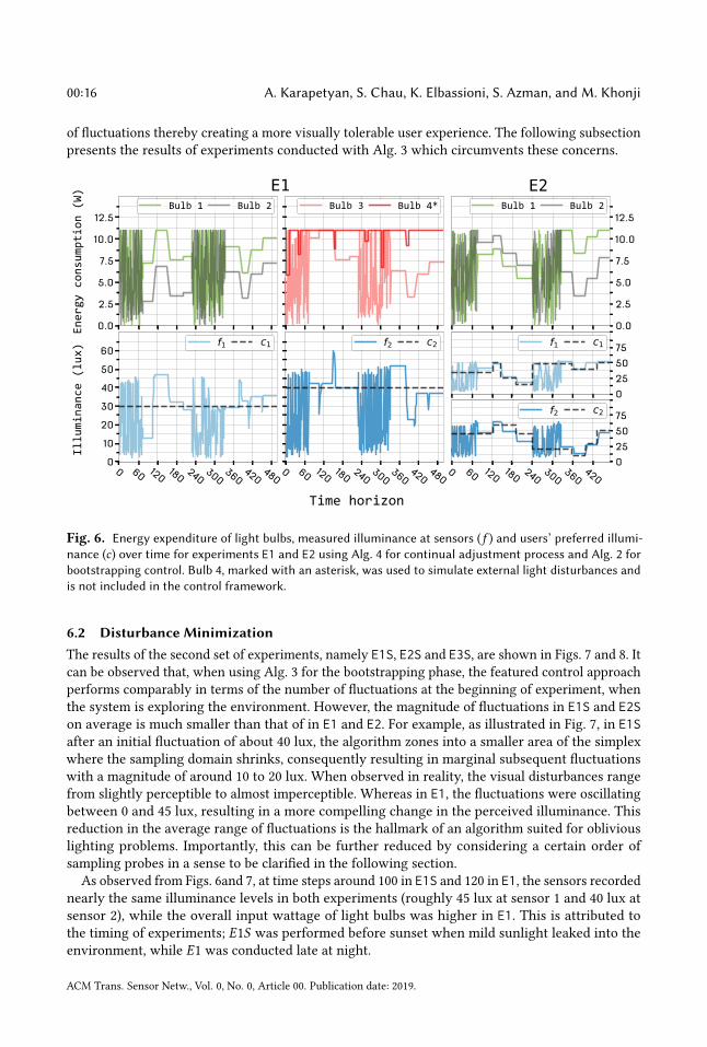
6.1 Smart Lighting with Oblivious SensorsThe results obtained from the first set of experiments, namely E1 and E2, are depicted in Fig. 6. As

can be inferred, the proposed approach, when Alg. 4 is invoked during the continual adjustment

stage and Alg. 2 for bootstrapping, proved successful at minimizing the total power consumption of

smart light bulbs without compromising users’ illuminance preferences. In E1, the system effectively

executed the continual adaptive adjustment algorithm to satisfy users’ preferences despite their

intensive mobility. Around time horizon 160 in E1, the sudden movement of user 2 towards a

light source resulted in a spike in the observed measurements, therein triggering the continual

adjustment routine, which rapidly modulated light bulbs’ input wattage as to meet the user’s

lighting requirements. Notice that the proposed approach prevailed despite the adversarial impact

of the simulated external light disturbances (the bulb marked with an asterisk in Fig. 6). Specifically,

subtly steeper descents are evident, as a result of the abrupt dimming, in E1 around time steps 160

and 375. Similarly, the employed approach also performed well throughout E2 by matching users’

heterogeneous requirements consistently without noticeably over- or under-illuminating.

Though Alg. 4 is expedient for small perturbations, it could fail to properly minimize the energy

wastage and meet users’ conflicting illuminance preferences in the events of significant illuminance

variations in the environment. Thus, in E1, when user 1 moved sufficiently far from a light source

at around time step 250, dropping the sensor readings from 28 lux to below 5 lux, the controller unit

initiated the bootstrapping phase. Also, the bootstrapping control served well in the beginning of the

experiments E1 and E2, when the system was completely oblivious to the deployment environment.

While the employed control strategy is commendable, it should be noted that the bootstrapping

stage is disconcerting as numerous large fluctuations of light bulbs accompany its sampling routine.

To the user, this translates to an unsettling period of random flashing of lights, even when smooth

lighting transitions are enabled. We remark that it is not necessarily the frequency of these fluctua-

tions but rather the sizable difference in the magnitude of these transitions that brings discomfort.

The culprit here is the design of Alg. 2, where sampling is performed over the entire simplex

domain, hence the frequent large changes in the light bulbs’ brightness (i.e., each bulb’s input

wattage takes values from 0% to 100%). As this questions practicality of the developed framework

in some applications, as is the case with smart lighting systems, it is vital to minimize the intensity



of fluctuations thereby creating a more visually tolerable user experience. The following subsection

presents the results of experiments conducted with Alg. 3 which circumvents these concerns.

0.0

2.5

5.0

7.5

10.0

12.5

E2Bulb 1 Bulb 2

0

25

50

75f1 c1

0 60 120180

240300

360420

0

25

50

75f2 c2

0.0

2.5

5.0

7.5

10.0

12.5

E1Bulb 1 Bulb 2 Bulb 3 Bulb 4*

0 60 120180

240300

360420

480

0

10

20

30

40

50

60f1 c1

0 60 120180

240300

360420

480

f2 c2

Time horizon

Ener

gy c

onsu

mpti

on (

W)Il

lumi

nanc

e (l

ux)

Fig. 6. Energy expenditure of light bulbs, measured illuminance at sensors (f ) and users’ preferred illumi-nance (c) over time for experiments E1 and E2 using Alg. 4 for continual adjustment process and Alg. 2 forbootstrapping control. Bulb 4, marked with an asterisk, was used to simulate external light disturbances andis not included in the control framework.

6.2 Disturbance MinimizationThe results of the second set of experiments, namely E1S, E2S and E3S, are shown in Figs. 7 and 8. It

can be observed that, when using Alg. 3 for the bootstrapping phase, the featured control approach

performs comparably in terms of the number of fluctuations at the beginning of experiment, when

the system is exploring the environment. However, the magnitude of fluctuations in E1S and E2Son average is much smaller than that of in E1 and E2. For example, as illustrated in Fig. 7, in E1Safter an initial fluctuation of about 40 lux, the algorithm zones into a smaller area of the simplex

where the sampling domain shrinks, consequently resulting in marginal subsequent fluctuations

with a magnitude of around 10 to 20 lux. When observed in reality, the visual disturbances range

from slightly perceptible to almost imperceptible. Whereas in E1, the fluctuations were oscillatingbetween 0 and 45 lux, resulting in a more compelling change in the perceived illuminance. This

reduction in the average range of fluctuations is the hallmark of an algorithm suited for oblivious

lighting problems. Importantly, this can be further reduced by considering a certain order of

sampling probes in a sense to be clarified in the following section.

As observed from Figs. 6and 7, at time steps around 100 in E1S and 120 in E1, the sensors recordednearly the same illuminance levels in both experiments (roughly 45 lux at sensor 1 and 40 lux at

sensor 2), while the overall input wattage of light bulbs was higher in E1. This is attributed to

the timing of experiments; E1S was performed before sunset when mild sunlight leaked into the

environment, while E1 was conducted late at night.



0.0

2.5

5.0

7.5

10.0

12.5

E2SBulb 1 Bulb 2

0

25

50

75f1 c1

0 40 80 120160

200240

280

0

25

50

75f2 c2

0.0

2.5

5.0

7.5

10.0

12.5

E1SBulb 1 Bulb 2 Bulb 3 Bulb 4*

0 40 80 120160

200240

280

0

10

20

30

40

50

60f1 c1

0 40 80 120160

200240

280

f2 c2

Time horizon

Ener

gy c

onsu

mpti

on (

W)Il

lumi

nanc

e (l

ux)

Fig. 7. Energy expenditure of light bulbs, measured illuminance at sensors (f ) and users’ preferred illumi-nance (c) over time for experiments E1S and E2S using Alg. 4 for continual adjustment process and Alg. 3 forbootstrapping control. Bulb 4, marked with an asterisk, was used to simulate external light disturbances andis not included in the control framework.

0.02.55.07.5

10.012.5 Bulb 1

0 90 180 270 3600.02.55.07.5

10.012.5 Bulb 2

Bulb 3

0 90 180 270 360

Bulb 4

Bulb 5

0 90 180 270 360

Bulb 6

Bulb 7

0 90 180 270 360

Bulb 8*

0 90 180 270 3600

25

50

75f1 c1

0 90 180 270 360

f2 c2

0 90 180 270 360

f3 c3

E3S

Time horizon

Ener

gy c

onsu

mpti

on (

W)Il

lumi

nanc

e (l

ux)

Fig. 8. Energy expenditure of light bulbs, measured illuminance at sensors (f ) and users’ preferred il-luminance (c) over time for experiment E3S using Alg. 4 for continual adjustment process and Alg. 3 forbootstrapping control. Bulb 8, marked with an asterisk, was used to simulate external light disturbances andis not included in the control framework.



The last experiment E3S, which results are pictured in Fig. 8, seeks to investigate the scalability

of the proposed approach on a larger scale instance with 7 light bulbs and 3 sensors. As in previous

experiments, the algorithm prevailed in meeting users’ heterogeneous illuminance preferences

while minimizing the net energy expenditure of smart light bulbs. Also, it displayed robustness

when presented with external abrupt light disturbances. In particular, the sharp drop in illuminance

brought by Bulb 8 was well handled at time step 280 along with the abrupt rise in illuminance at

time step 390. However, the bootstrapping phase witnessed a longer period of fluctuations in E3S ascompared to E2S and E1S, signifying that the algorithm explored a larger sampling space. Despite

this, the featured control algorithm managed to reach a solution within plausible time frame, thus

confirming its scalability in larger problem spaces.

7 DISCUSSIONSWhile the deployed testbed prototype demonstrates the empirical effectiveness of the proposed

smart lighting control approach, further improvement can be attained, for user comfort and perfor-

mance, through auxiliary hardware upgrades. This section elaborates on the latter aspect as well as

suggests promising directions for future work.

7.1 Hardware ImprovementsIn Section 3, an efficient strategy was introduced to attenuate the visual discomfort and disturbance

to users during the bootstrapping control phase. Below, we list several possible solutions, on the

hardware side, to further enhance user comfort and experience as well as expand the system’s

functionalities.

(1) Improved Sensors and Light Bulbs: The implemented testbed prototype relies on Android

smartphones and LIFX smart light bulbs connected through a wireless local network.Whereas,

it is possible to design specific wearable devices with improved light sensors and dedicated

communication network that have faster reaction time and refined communication capa-

bilities. This will minimize the latency in data transfer between sensors, smart light bulbs

and monitoring unit. Moreover, future smart light bulbs are expected to be equipped with

improved power electronics allowing rapid brightness adjustments, which will further reduce

the control lags.

(2) Wearable Sensors with Accelerometers: To improve the performance of control algorithm, we

can incorporate the accelerometer readings in mobile devices that are embedded with light

sensors. For example, if there are slower changes in the motion of sensors, then the control

system will execute the continual adjustment algorithm in a slow pace. If there are more

rapid changes in the motion of sensors, then the continual adjustment algorithm will be

executed in a faster pace. In general, it will be an interesting future study to integrate the

accelerometer readings in the control system for more effective smart lighting control.

7.2 Color AdjustmentsThe present study demonstrates the effectiveness of intelligent lighting control system empirically

in a real-world environment. However, the featured control approach can be also applied to a more

sophisticated setting ofmulti-color illuminance control [2]. For example, users can set heterogeneous

preferences on the color temperature. Different colors exhibit distinct radiation effects: reddish

colors create warmer effect to the human eye, while bluish ones colder. It is well-known that warmer

colors are more pleasant to humans in dim environment, whereas colder colors are better for bright

environment. Also, users may have different psychological preferences to color temperature. Hence,



given these heterogeneous preferences, the perceived objective would be to coordinate the color

and brightness adjustments of smart light bulbs at their lowest possible energy expenditure.

8 CONCLUDING REMARKSThis article studied a practical application of an IoT-empowered sensing and actuation system for

smart lighting control with oblivious mobile sensors, which enables adaptive control in real-time

without the complete knowledge of the dynamic uncertain environment. The featured system

has been implemented in a prototype testbed, using programmable smart light bulbs and light

sensors in smartphones, deployed in a real-world indoor environment. We presented a novel model

formulation, capturing general oblivious multi-sensor IoT applications by a generic framework,

yielding a robust control framework agnostic to deployment environment and the associated

parameters. With this model, we devised efficient algorithms that minimize the total energy

expenditure of smart light bulbs, while meeting users’ heterogeneous illuminance requirements. The

proposed algorithms were applied to the testbed and their effectiveness was validated extensively

under diverse settings and scenarios. Lastly, we discussed some potential improvements on the

hardware side along with promising directions for future work.

AcknowledgmentsWe gratefully acknowledge the valuable comments and suggestions provided by the ACM BuildSys

2018 program committee chairs (Polly Huang and Marta Gonzalez), shepherd (Romil Bhardwaj),

and anonymous reviewers.

APPENDIXThe appendix sketches the theoretical foundations for Algs. 2 and 3 followed by a detailed list of all

improvements and extensions upon the preliminary variant of this study in [9]. We also include

the theoretical proof for completeness.

Analytical Underpinnings of the Bootstrapping AlgorithmsRecall that Algs. 2 and 3, in producing close to optimal approximately feasible solutions to LCP2[B],seek to tackle its counterpart of the form of:

λ⋆[B] = min{Λ(p) | p ∈ P}, (7)

where Λ(p) = max

{ ∑nj=1 pj

∑mi=1 f

ti, j (x

ti ) | x

t ∈ S(B)}and P = {p ∈ Rn+ |

∑nj=1 pj = 1}. As

mentioned previously, both algorithms borrow from the Lagrangian decomposition scheme of [7].

Accordingly, the proceeding analysis follows closely the lines laid out therein.

The employed decomposition, put simply, is an iterative strategy that approaches LCP2[B] viaits Lagrangian dual by computing pairs of vectors p,x successively in the following manner. Given

the current x ∈ S(B), the algorithm generates a set of weights p ∈ P corresponding to the coupling

constraints (3). For this p, it then computes an approximate solution x̂ of Λ(p), and moves from xto (1 − τ )x + τ x̂ with a suitable step length τ ∈ (0, 1].

The cornerstone of this method relies on attributing to the covering constraints (3) a logarithmicpotential function of the form

Φ(θ , f ) = lnθ +ξ

n

n∑j=1

ln(f tj (xt ) − θ ) , (8)



where θ ∈ R, f = (f tj )j ∈N are variables and ξ is a fixed positive parameter proportionate to the

accuracy tolerance η in Algs. 2 and 3. Note that Φ is well defined for 0 < θ < λ(f ) , minj ∈N{ ftj }

and its maximizer θ (f ) emerges from the first-order optimality condition

ξθ

n

n∑j=1

1

f tj (xt ) − θ

= 1 , (9)

which has a unique solution as its left-hand side is a strictly increasing function of θ . Then the

logarithmic dual vector (weights) can be defined as

pj =ξ

n

θ (f )

f tj (xt ) − θ (f )

∀ j ∈ N , (10)

since now p ∈ P by (9). On these grounds, the following Lemma is formulated.

Lemma 1 ([7]). Let η ∈ (0, 1), ξ = η6and p be derived from (10) for a given x ∈ S(B). Suppose

an approximate solution x̂ ∈ S(B) to Λ(p) is computed such that∑n

j=1 pj ftj (x̂) ≥ (1 − ξ )Λ(p). If

µ =

∑nj=1 pj f

tj (x̂) −

∑nj=1 pj f

tj (x)∑n

j=1 pj ftj (x̂) +

∑nj=1 pj f

tj (x)

≤ ξ , then x is an approximately feasible solution to LCP2[B]

satisfying∑m

i=1 fti, j (x) ≥ (1 − η)λ

⋆[B] for ∀j ∈ N .

Proof. Rewrite the condition µ ≤ ξ as

(1 − ξ )n∑j=1

pj ftj (x̂) ≤ (1 + ξ )

n∑j=1

pj ftj (x) . (11)

Observe that

n∑j=1

pj ftj (x) =

n∑j=1

ξ

n

θ (f )f tj (x)

f tj (x) − θ (f )(12)

=ξθ (f )

n

n∑j=1

f tj (x)

f tj (x) − θ (f )(13)

=ξθ (f )

n

n∑j=1

(1 +

θ (f )

f tj (x) − θ (f )

)(14)

= ξθ (f ) + θ (f )n∑j=1

pj (15)

= (1 + ξ )θ (f ) . (16)

Since

∑nj=1 pj f

tj (x̂) ≥ (1 − ξ )Λ(p), from (11) and (16) it follows that

(1 − ξ )2Λ(p) ≤ (1 + ξ )2θ (f ) . (17)



This, in conjunction with the facts that θ (f ) < λ(f ), Λ(p) ≥ λ⋆[B], yields

λ⋆[B] ≤ Λ(p) (18)

≤(1 + ξ )2

(1 − ξ )2θ (f ) (19)

≤ (1 + η)λ(f ) (20)

≤λ(f )

(1 − η), (21)

(22)

thus concluding the proof. �

Remark. In approximating Λ(p), Algs. 2 and 3 resort to the sampling-based subroutine as a proxymeasure since direct approaches are computationally prohibitive. Though efficient, this samplingprocedure does not necessarily guarantee the assumption

∑nj=1 pj f

tj (x̂) ≥ (1 − ξ )Λ(p) of Lemma 1

holds. Yet, for the current application and settings, this condition tends to be oftentimes satisfied throughsufficiently large sample cohorts, hence the empirical success of Algs. 2 and 3.

Summary of ChangesThe following list presents the new enhancements and extensions added to the current version,

with respect to the preliminary version in [9]:

(1) Section 4, which presents the proposed smart lighting control algorithms, has been extended

with a completely new subsection (Subsection 4.2) that more thoroughly addressed the

potential visual disturbance to users during the bootstrapping phase. Also, a new lighting

control has been devised in Alg. 3. We have implemented the new algorithms in our testbed

prototype.

(2) The experimental setup and the deployed smart lighting testbed, laid out in Section 5, have

been improved in the followingways. To account for external light disruptions in the proposed

setup, one of the smart light bulbs was modeled to simulate abrupt light changes in the testbed

environment through random flickering at certain points during the course of experiments.

Additionally, the graphical interface of the developed smartphone application has been refined

to facilitate user experience.

(3) Section 6, which validates the featured smart lighting control approach empirically, has

been revised completely with the results of all new experiments performed in a different

deployment environment with an updated set of experimental scenarios using our new

testbed prototype implementation.

(4) For the sake of completeness, we have included an appendix explaining the theoretical

foundations behind the proposed bootstrapping control algorithms.

(5) We have conducted a more comprehensive literature review including several additional

related works in Section 2.

(6) Abstract, Introduction (Section 1) and Problem Formulation (Section 3) sections have been

also substantially revised.



REFERENCES[1] Muhammad Aftab, Chien Chen, Chi-Kin Chau, and Talal Rahwan. 2017. Automatic HVAC control with real-time

occupancy recognition and simulation-guided model predictive control in low-cost embedded system. Energy andBuildings 154 (2017), 141 – 156.

[2] Simon HA Begemann, Ariadne D Tenner, and Gerrit J Van Den Beld. 1998. Lighting system for controlling the color

temperature of artificial light under the influence of the daylight level. US Patent 5,721,471.

[3] Dimitris Bertsimas and Santosh Vempala. 2004. Solving convex programs by random walks. Journal of ACM 51, 4

(2004), 540–556.

[4] Peter Robert Boyce. 2014. Human factors in lighting. Crc Press.[5] D Caicedo, S Li, and A Pandharipande. 2017. Smart lighting control with workspace and ceiling sensors. Lighting

Research & Technology 49, 4 (2017), 446–460.

[6] Meghan Clark. 2018. Python Library for Accessing LIFX Devices Locally Using the Official LIFX LAN Protocol.

https://github.com/mclarkk/lifxlan.

[7] M. D. Grigoriadis, L. G. Khachiyan, L. Porkolab, and J. Villavicencio. 2001. Approximate Max-Min Resource Sharing

for Structured Concave Optimization. SIAM Journal on Optimization 11, 4 (2001), 1081–1091.

[8] Adam Kalai and Santosh Vempala. 2006. Simulated Annealing for Convex Optimization. Mathematics of OperationsResearch 31, 2 (2006), 253–266.

[9] Areg Karapetyan, Sid Chi-Kin Chau, Khaled Elbassioni, Majid Khonji, and Emad Dababseh. 2018. Smart Lighting

Control Using Oblivious Mobile Sensors. In Proceedings of the 5th Conference on Systems for Built Environments (BuildSys’18). ACM, New York, NY, USA, 158–167. https://doi.org/10.1145/3276774.3276788

[10] M. T. Koroglu and K. M. Passino. 2014. Illumination Balancing Algorithm for Smart Lights. IEEE Transactions onControl Systems Technology 22, 2 (March 2014), 557–567.

[11] László Lovász and Santosh Vempala. 2004. Hit-and-run from a corner. In ACM Symposium on Theory of Computing(STOC). 310–314.

[12] László Lovász and Santosh Vempala. 2006. Fast Algorithms for Logconcave Functions: Sampling, Rounding, Integration

and Optimization. In IEEE Annual Symposium on Foundations of Computer Science (FOCS). 57–68.[13] László Lovász and Santosh Vempala. 2006. Hit-and-run from a corner. SIAM J. Comput. 35, 4 (2006), 985–1005.[14] M. Miki, A. Amamiya, and T. Hiroyasu. 2007. Distributed optimal control of lighting based on stochastic hill climbing

method with variable neighborhood. In 2007 IEEE International Conference on Systems, Man and Cybernetics. 1676–1680.https://doi.org/10.1109/ICSMC.2007.4413957

[15] Dennis E. Phillips, Rui Tan, Mohammad-Mahdi Moazzami, Guoliang Xing, Jinzhu Chen, and David K. Y. Yau. 2013.

Supero: A Sensor System for Unsupervised Residential Power Usage Monitoring. In IEEE International Conference onPervasive Computing and Communications (PerCom).

[16] Vipul Singhvi, Andreas Krause, Carlos Guestrin, James H. Garrett, Jr., and H. Scott Matthews. 2005. Intelligent Light

Control Using Sensor Networks. In ACM Conference on Embedded Networked Sensor Systems (SenSys).[17] Noah A Smith and Roy W Tromble. 2004. Sampling uniformly from the unit simplex. Johns Hopkins University, Tech.

Rep 29 (2004).

[18] Niels van de Meugheuvel, Ashish Pandharipande, David Caicedo, and PPJ Van Den Hof. 2014. Distributed lighting

control with daylight and occupancy adaptation. Energy and Buildings 75 (2014), 321–329.[19] Yao-Jung Wen and A. M. Agogino. 2008. Wireless networked lighting systems for optimizing energy savings and user

satisfaction. In IEEE Wireless Hive Networks Conference. 1–7.[20] Y-J. Wen and A. M. Agogino. 2011. Control of wireless-networked lighting in open-plan offices. Lighting Research &

Technology 43, 2 (2011), 235–248.

[21] Lun-Wu Yeh, Che-Yen Lu, Chi-Wai Kou, Yu-Chee Tseng, and Chih-Wei Yi. 2010. Autonomous light control by wireless

sensor and actuator networks. IEEE Sensors Journal 10, 6 (2010), 1029–1041.[22] S. A. R. Zaidi, A. Imran, D. C. McLernon, and M. Ghogho. 2014. Enabling IoT empowered smart lighting solutions: A

communication theoretic perspective. In 2014 IEEE Wireless Communications and Networking Conference Workshops(WCNCW). 140–144. https://doi.org/10.1109/WCNCW.2014.6934875

[23] Nan Zhao, Matthew Aldrich, Christoph F. Reinhart, and Joseph A. Paradiso. 2015. A Multidimensional Continuous

Contextual Lighting Control System Using Google Glass. In ACM International Conference on Embedded Systems forEnergy-Efficient Built Environments (BuildSys). 235–244.


https://github.com/mclarkk/lifxlan

https://doi.org/10.1145/3276774.3276788

https://doi.org/10.1109/ICSMC.2007.4413957

https://doi.org/10.1109/WCNCW.2014.6934875

Documents

Multi-sensor Adaptive Control System for IoT-empowered