Multi Scale Color Coding of Fluid Flow Mixing Indicators

Multi Scale Color Coding of Fluid Flow Mixing Indicatorsalong Integration Lines

Sandeep Khurana

Department of Computer Science1

Center for Computation & Technology1

[email protected]

Nathan Brener

Bijaya Karki

Department of Computer Science1

[email protected]

[email protected]

Werner Benger

Center for Computation & Technology1

Institute for Astro- and Particle Physics2

[email protected]

[email protected]

Somnath Roy4

Sumanta Acharya1

Dept. of Mechanical Engineering

[email protected]

[email protected]

Marcel Ritter

Inst. of Basic Sciences in Civil Engineering2

[email protected]

S. Sitharama Iyengar

School of Computing & Info. Sciences3

[email protected]

ABSTRACT

This paper presents a multi scale color coding technique which enhances the visualization of scalar fields along integrationlines in vector fields. In particular, this multi scale technique enables one to see detailed variations in selected small rangesof the scalar field while at the same time allowing one to observe the entire range of values of the scalar field. This typeof visualization, observing small variations as well as the entire range of values, is usually not possible with uniform colorcoding. This multi scale approach, which is linear within each division of the scale (piecewise linear), is a general visualizationtechnique that can be applied to many different scalar fields of interest. As an example, in this paper we apply it to thevisualization of fluid flow mixing indicators along pathlines in computational fluid dynamics (CFD) simulations. Pathlinesare the trajectories of fluid particles over time in the CFD simulations, and applying multi scale color coding on the pathlinesbrings out quantities of interest in the flow such as curvature, torsion and specific measure of length generation, which areindicators of the degree of mixing in the fluid system. In contrast to uniform color coding, this multi scale scheme can displaysmall variations in the mixing indicators and still show the entire range of values of these indicators. In this paper, the mixingindicators are computed and displayed only along line structures (pathlines) in the flow field rather than at all points in the flowfield.

Keywords: transfer function generation, pathlines, nonlinear color map, computational fluid dynamics, vectorfield visualization, mixing indicators

1 INTRODUCTION1.1 MotivationThis paper proposes a multi scale color coding schemewhich can display nonuniform distributions of quanti-ties that have small variations in some ranges and larger

Permission to make digital or hard copies of all or part ofthis work for personal or classroom use is granted withoutfee provided that copies are not made or distributed for profitor commercial advantage and that copies bear this noticeand the full citation on the first page. To copy otherwise,or republish, to post on servers or to redistribute to lists,requires prior specific permission and/or a fee.

1 Louisiana State University, Baton Rouge, LA-70803, USA2 University of Innsbruck, Technikerstraße 25/8, A-6020 Innsbruck,

Austria3 Florida International University, Miami, FL-33199, USA4 Indian Institute of Technology, Patna, India

variations in other ranges. The paper shows the advan-tages of this multi scale technique compared to uniformcolor coding which usually cannot display both smalland large variations in the same image. In this multiscale approach, the overall scale is divided up into in-tervals specified by the user, with a different linear scaleinside each interval (i.e., it is piecewise linear). Thistechnique enables one to see small variations in selectedranges of the quantity of interest and also observe theentire range of values of this quantity. This multi scalescheme is a general technique that can be used to visu-alize any scalar quantity of interest. As an example ofthis method, we use it to visualize fluid mixing indica-tors along integration lines (pathlines) in computationalfluid dynamics simulations of fluid flow. In this paperthe mixing indicators are computed and displayed onlyalong the pathlines rather than at all points in the flowfield.

WSCG 2012 Communication Proceedings 357 http://www.wscg.eu

Computational fluid dynamics (CFD) uses numeri-cal methods and analysis techniques to study fluid flow.The computational results from numerical models canyield data which is on the order of hundreds of giga-bytes and consists of multiple blocks containing mil-lions of cells. Computation on such a grid can take asubstantial amount of time to trace the paths of fluidparticles over time (pathlines). But once these pathlineshave been calculated, fluid mixing indicators, such ascurvature and torsion, can then be quickly computedand visualized at every point on the pathlines. Cur-vature and torsion computations along pathlines in astirred tank CFD simulation were done earlier [3] anduniformly color coded, but the distribution of these val-ues is not uniform. In this paper the multi scale colorcoding technique is used to display the nonuniform dis-tributions of these quantities. The paper also adds an-other mixing indicator, the specific measure of lengthgeneration, to complement the curvature and torsion soas to better understand the mixing. In addition it useshigher order difference formulas to improve the accu-racy of the curvature and torsion calculations. As men-tioned above, the multi scale color coding scheme is ageneral method that can be used to visualize any scalarfield of interest, such as pressure, which is also shownin the paper.

1.2 Fluid Mixing IndicatorsIn order to develop an understanding of the mechani-cal macro mixing process, we investigate the motion ofthe fluid particles in the flow domain. The flow domainconsidered is a mechanically agitated turbulent stirredtank with down-pumping pitched blade impellers. Wa-ter is considered as the working fluid in which a blob ofa tracer is injected at a particular location. We look intothe pathlines of a number of points associated with theinjected tracer. These pathlines show exactly how tracerparticles move inside the stirred tank volume. Fromthe pathline visualizations, we try to qualitatively un-derstand the stretching and distortions on the fluid ele-ments by calculating the curvature and torsion at dif-ferent points along the pathlines. A higher value ofthe curvature indicates more straining of the fluid el-ement associated with it and also higher residence timeof the fluid particle in that particular region resulting inprolonged inter-diffusion of the fluids, which promotesmixing [12]. The torsion is a measure of twisting strainson the fluid elements which also promotes the break upof the clumps and enhances mixing. Torsion can be pos-itive or negative, but the degree of mixing in the stirredtank depends primarily on the magnitude of the torsionrather than its sign. Therefore, for visualizing torsion,we will show its absolute value (magnitude), neglectingwhether the twist is clockwise or counterclockwise.

The curvature κ and torsion τ are given by

κ =|q̈× q̇||q̇|3

. (1)

τ =

...q · (q̈× q̇)

|q̈× q̇|2. (2)

where q̇ is the velocity of the fluid (vector field) and q̈and

...q are the first and second derivatives of the vectorfield with respect to time. In our approach we com-pute pathlines from the vector field first, based on user-specified initially defined seeding points, and then cal-culate curvature and torsion along the pathlines as apost-processing step.

Another measure of fluid mixing is the specific mea-sure of length generation [13] defined as

d ln(λ )dt

(3)

where λ = δ

L , δ being the increase in path length (whichis proportional to the magnitude of the velocity) and Lbeing the total path length (before the δ increment) ata particular time t. The proportional change of the pathlength will be larger at the start of the pathlines andsmaller at their ends, thus this mixing indicator will bedominated by variations of the velocity as the pathlinesget longer. The greater the specific measure of lengthgeneration, the greater the mixing. This quantity is alsocalculated as a post-processing step on the pathlines. Itshould be noted that in addition to the mixing indicatorsdescribed above, there are also other principles that canbe used to investigate the mixing of fluids.

1.3 Related WorkAutomated generation of color maps has been the sub-ject of research in scientific visualization for decades.Yet, still many visualization tools rely on manual spec-ification of colors as the problem is highly applicationand problem specific. Taking over full control of colormap generation from the user is usually not even desir-able, leaving semi-automated assistance of color spec-ification as the best compromise. A well known ap-proach is the method of finding material boundaries byG. Kindlmann [8]. In this approach a Histogram Vol-ume Structure is created which measures the relation-ship between the data values and their derivatives. Inthis volume, the three axes are f , f ′ and f ′′ , each axisis divided into some number of bins which contains thenumber of voxels falling in the same combination ofranges of these variables. This information facilitates ahigh-level interface to opacity function creation. In thewinning entry of the IEEE Visualization 2004 Contest[6], the visualization system VisSym was highlighted,where the subset of data items were manually selectedusing techniques for information visualization such asscatter plots and histograms. These values were related


to the dataset, e.g., for detecting the eye of the hurri-cane area, cells which exhibit low velocity and pressureregions were brushed out.

Our main objective is the depiction of scalar-valuedfluid flow mixing indicators along pathlines. Fluid flowquantities such as curvature and torsion are commonsubjects of study. Weinkauf [15] demonstrated compu-tation of curvature and torsion as a field over the entiredata domain, allowing one to identify regions of interestwithin the full spatial domain. Due to the sheer amountof dynamic data in our application, which comprisesabout 300GB of binary data, this approach is not feasi-ble and we need to restrict ourselves to displaying suchfield quantities on precomputed pathlines. One methodfor doing this is to use a geometric object [5] to visual-ize the fluid fields along the pathlines, however, if thenumber of pathlines is large, this approach is not vi-sually appealing because the image is more clutteredand does not give global information about the flow. Inthe approach proposed here, we employ a simple butefficient way to display data values with a wide numer-ical range by specifying color mapping via histogrampercentage rather than absolute data values. Render-ing of these pathlines using the illuminated streamlinesmethod [17] gives a 3D view of the lines using PhongShading. The depth perception can be further enhancedby using the halos described in [7, 11] and we plan toimplement this halo feature in future work on color cod-ing line structures.

2 OUR APPROACHThe vector field in the stirred tank simulations producedscalar fields, such as curvature and torsion, which havea wide range of values in some parts of the stirred tank.The use of uniform color coding for the whole rangeof these scalar values often gives a single predominantcolor along most of the length of the pathlines, makingit impossible to visualize small variations in these val-ues. This paper describes the use of a multi scale colorcoding scheme which not only shows small variationsin the scalar field but also enables one to see the en-tire range of values of the scalar field by just looking atthe color coded pathlines. In this paper, the curvatureand torsion, and also a new mixing indicator, the spe-cific measure of length generation, are calculated for300 time steps using more accurate higher order differ-ence formulas and are then visualized using the multiscale color coding technique. Also another scalar quan-tity of interest, the pressure, is visualized using this ap-proach. This multi scale color coding scheme enablesone to easily draw conclusions about the behavior ofthe scalar fields without any uncertainty about the vari-ations in the small values.

2.1 Higher Order Differentiation SchemesThe formulas for the curvature, eqn. (1), and torsion,eqn. (2), contain the first and second derivatives ofthe velocity with respect to time, and the specific mea-sure of length generation is defined as the first deriva-tive of ln(λ ) with respect to time, eqn. (3). In thiswork we computed these derivatives with more accu-rate higher order difference formulas compared to pre-vious work [3, 4]. We used the following central differ-ence formulas with fourth order accuracy for the firstand second derivatives:

f ′(x0)≈

(1

12f (x−2)−

23

f (x−1)+

23

f (x1)−1

12f (x2)

)/hx (4)

f ′′(x0)≈

(− 1

12f (x−2)+

23

f (x−1)−52

f (x0)

+43

f (x1)−1

12f (x2)

)/h2

x (5)

2.2 Multi Scale Color CodingDesigning a multi scale for color coding depends onseveral parameters like the number of divisions in thescale, the range of the scalar values in each division andthe selection of the color range for each division. Gen-erally one needs to visualize the entire range of scalarfield values including small, medium and large values,but if the range of values is large, as in the case of cur-vature and torsion, uniform color coding often gives asingle predominant color for most of the pathline whichmakes it difficult to distinguish between these values.For the mixing indicators described in this paper, weneed to see the small and medium values in addition tothe large values in order to determine where the mixingspeed in the stirred tank is slow, intermediate and fast.Once the ranges of scalar values that need to be visual-ized in detail have been determined, one can then spec-ify the number of divisions in the multi scale and therange of values and the color range for each division.There are a few considerations for the colors [9,16] thatneed to be addressed, including the fact that the humaneye perceives more variation in the green than in theother colors. As an example of this, Figs. 6 and 7 con-tain a lot of green which enables one to readily see thevariations in the scalar values. Other than these consid-erations, the colors can generally be chosen as the userdesires.

Various techniques can be used to construct the multiscale. In the method presented here, the number of di-visions in the multi scale and the range of scalar values


in each division are determined manually so as to fa-cilitate the visualization of the scalar field variations ofinterest. A cumulative histogram of the scalar valuesis used to determine the boundaries of the divisions sothat each one contains the desired percentage of scalarvalues. In this paper, all of the multi scales have threedivisions and the same range of colors, but these arejust examples to illustrate the multi scale method. Ingeneral the user can choose any number of divisionsand specify any range of scalar values and any range ofcolors for each division in order to enhance the visual-ization of the scalar values of interest. Currently thisprocess is not automated but rather is done manually bythe user. There also exists other work in this area whichdescribes ways to come up with ranges of values fromthe scalar field. These involve automatic [10], semi-automatic [8] and manual generation of the functions todo this task [14].

Here, since we need to visualize small, medium andlarge values of the scalar field, three divisions were se-lected for the multi scale color coding. An example ofthese three divisions is given in Fig. 1, where the first,second and third divisions go from 0% to 10%, 10%to 30%, and 30% to 90% of the scalar values, and thethird division is capped at 90%, with values above 90%being set to the 90% value. Capping the third divisionat 90% enables one to see the variation of the valuesbetween 30% and 90% in greater detail, which is morerelevant to the mixing process than the variation of thelarge values between 90% and 100%. Each divisionhas linear color gradients of R, G and B going from theleft end point to the right end point of the division, butthe overall color variation over all three divisions is notuniform but rather is multi scale in order to better showthe variations in the small and medium scalar values.In the example shown in Figure 1, in the first division Rvaries linearly from 0 to 255, G=0, and B varies linearlyfrom 255 to 0, in the second division R=255, G varieslinearly from 0 to 255, and B=0, and in the third divi-sion R varies linearly from 255 to 0, G=255, and B=0.These color ranges for the three divisions were used tocolor code all four of the scalar fields shown in the pa-per, while the percents used for the boundaries betweenthe divisions were different for each scalar field.

Figure 1: An example of Multi Scale Color Codingwith different ranges of scalar values to distinguish re-gions of low values and medium values.

2.3 RenderingFor the final rendering step, we employ the method ofilluminated streamlines [17], which provides improveddepth perception as compared to homogeneously col-ored lines. While in its original form only monochromeillumination could be supported by OpenGL 1.0 hard-ware, modern OpenGL implementations support multi-texturing and thus allow an additional one-dimensionallighting model as proposed in [17]. Illumination oflines is done by using the Phong Reflection modelwhich defines the intensity (I) at any point as

I = Iambient + Idi f f use + Ispecular

= ka + kdL ·N + ks(V ·R)n (6)

where L denotes the light direction, V the viewing di-rection and R the unit reflection vector (the vector in theL-N-plane with the same angle to the surface normal asthe incident light). ka, kd and ks are the ambient, dif-fuse and specular reflection constants respectively. Forlines the normals and reflection vectors are undefined.So, intensity can be made dependent on the tangentialvector T instead as

L ·N = |LN |=√

1− (L ·T )2 (7)

and

V ·R =(L ·T )(V ·T )−√1− (L ·T )2

√1− (V ·T )2 . (8)

In order to enhance the color resolution, we use proce-dural color maps that are merely parametrized throughlinear functions between each key value. Generally,this linear mapping will be sufficient for each range ofscalar values, but if a particular range needs to be sub-divided, then that particular range can have more thanone linear scale and additional colors. In the approachwe have discussed, some idea of the scalar values canbe derived from the histogram where, if more pointsare biased to a single value in that range, then nonlinearfunctions can be applied to map values to color for thesingle range. Only at the rendering step is the color mapdiscretized into a texture, for instance one with 256 en-tries if sufficient, but a higher color resolution can beused if required.

3 RESULTSWe used the the multi scale color coding technique de-scribed above to color code the pathlines in the stirredtank. The main idea is to visualize the pathlines andcolor code them with different scalar quantities that in-dicate the mixing of the fluids. The quantities that werecolor coded are curvature, torsion, specific measure oflength generation, and pressure. These are shown inseparate sections which compare the uniform and multi


scale color coding methods for each quantity. The path-lines are generated by introducing 36 seeding points or516 seeding points on two spheres placed symmetri-cally about the z-axis in the stirred tank and traced for300 timesteps totaling about 1.8 secs.

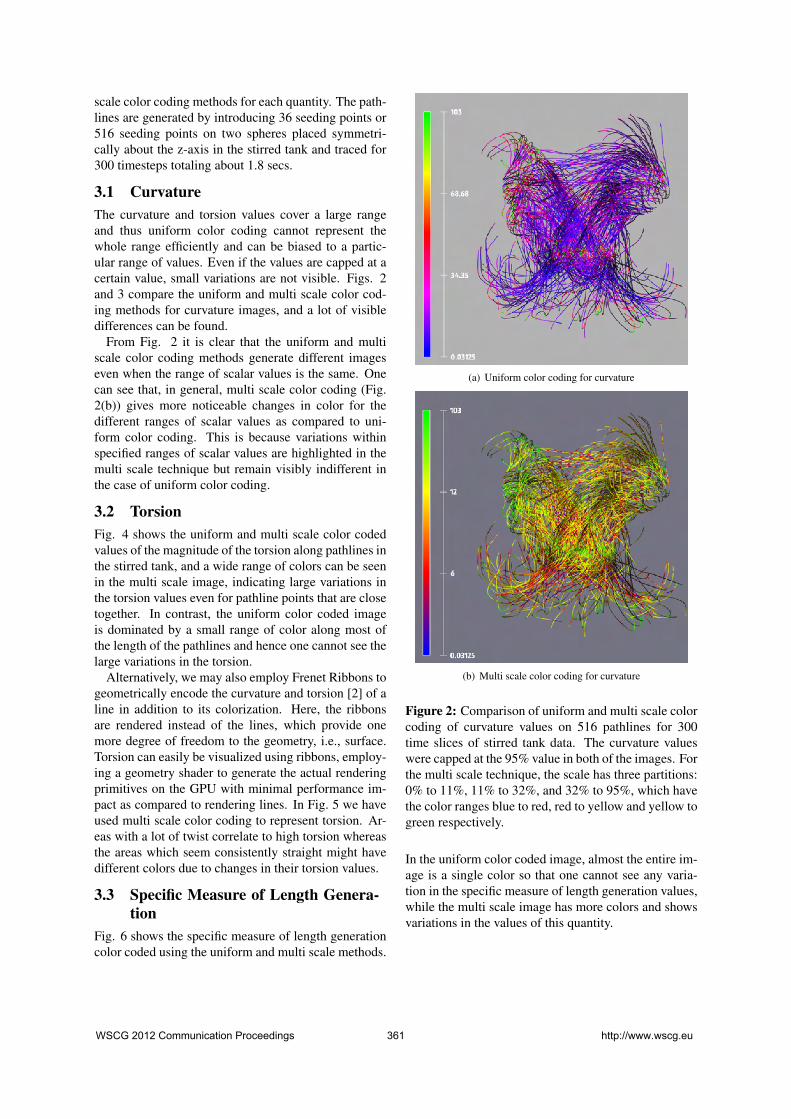
3.1 CurvatureThe curvature and torsion values cover a large rangeand thus uniform color coding cannot represent thewhole range efficiently and can be biased to a partic-ular range of values. Even if the values are capped at acertain value, small variations are not visible. Figs. 2and 3 compare the uniform and multi scale color cod-ing methods for curvature images, and a lot of visibledifferences can be found.

From Fig. 2 it is clear that the uniform and multiscale color coding methods generate different imageseven when the range of scalar values is the same. Onecan see that, in general, multi scale color coding (Fig.2(b)) gives more noticeable changes in color for thedifferent ranges of scalar values as compared to uni-form color coding. This is because variations withinspecified ranges of scalar values are highlighted in themulti scale technique but remain visibly indifferent inthe case of uniform color coding.

3.2 TorsionFig. 4 shows the uniform and multi scale color codedvalues of the magnitude of the torsion along pathlines inthe stirred tank, and a wide range of colors can be seenin the multi scale image, indicating large variations inthe torsion values even for pathline points that are closetogether. In contrast, the uniform color coded imageis dominated by a small range of color along most ofthe length of the pathlines and hence one cannot see thelarge variations in the torsion.

Alternatively, we may also employ Frenet Ribbons togeometrically encode the curvature and torsion [2] of aline in addition to its colorization. Here, the ribbonsare rendered instead of the lines, which provide onemore degree of freedom to the geometry, i.e., surface.Torsion can easily be visualized using ribbons, employ-ing a geometry shader to generate the actual renderingprimitives on the GPU with minimal performance im-pact as compared to rendering lines. In Fig. 5 we haveused multi scale color coding to represent torsion. Ar-eas with a lot of twist correlate to high torsion whereasthe areas which seem consistently straight might havedifferent colors due to changes in their torsion values.

3.3 Specific Measure of Length Genera-tion

Fig. 6 shows the specific measure of length generationcolor coded using the uniform and multi scale methods.

(a) Uniform color coding for curvature

(b) Multi scale color coding for curvature

Figure 2: Comparison of uniform and multi scale colorcoding of curvature values on 516 pathlines for 300time slices of stirred tank data. The curvature valueswere capped at the 95% value in both of the images. Forthe multi scale technique, the scale has three partitions:0% to 11%, 11% to 32%, and 32% to 95%, which havethe color ranges blue to red, red to yellow and yellow togreen respectively.

In the uniform color coded image, almost the entire im-age is a single color so that one cannot see any varia-tion in the specific measure of length generation values,while the multi scale image has more colors and showsvariations in the values of this quantity.


(a) Uniform color coding for curvature

(b) Multi scale color coding for curvature

Figure 3: Comparison of uniform and multi scale colorcoding of curvature values on 36 pathlines for 300 timeslices of stirred tank data. The curvature values werecapped at the 95% value in both of the images. For themulti scale technique, the scale has three partitions: 0%to 11%, 11% to 32%, and 32% to 95%, which have thecolor ranges blue to red, red to yellow and yellow togreen respectively.

3.4 PressureThe pressure field is a scalar quantity of interest whichis given at all of the grid points in the stirred tank simu-lation data set. Fig. 7 displays the values of the pressureusing the uniform and multi scale color coding meth-ods. As in Fig. 6, the uniform image is mostly a singlecolor and thus shows very little variation in the pres-

(a) Uniform color coding for torsion

(b) Multi scale color coding for torsion

Figure 4: Comparison of uniform and multi scale colorcoding of torsion values on 516 pathlines for 300 timeslices of stirred tank data. The values were capped atthe 90% value in both the images. For the multi scaletechnique, the scale has three divisions: 0% to 15%,15% to 40% and 40% to 90%, which have the colorranges blue to red, red to yellow and yellow to green.

sure, while the multi scale image has more colors andshows significant variations in the pressure.

4 DOMAIN EXPERT REVIEWImages for all of the fluid mixing indicators consid-ered here are generated using both the multi scale andthe uniform color coding techniques. The multi scaleimages can be observed for analysis of mixing perfor-mance as they are capable of displaying both the well


Figure 5: Multi scale color coding of torsion values onthe pathlines visualized as ribbons. Values used to colorcode are the same as in Fig. 4(b)

and poorly mixed zones. The larger values of the tor-sion, curvature or specific measure of length generationof the pathlines indicate the areas where the mixing isgreater. There are some lines which can be observedto have the same green color in all of the multi scaleimages, indicating high mixing along that particular lo-cus of the tracer particle. Similarly, certain lines canbe found which have low values for all three mixingfactors, indicating lower mixing in those regions of thestirred tank. These types of observations are not possi-ble in the corresponding uniformly color coded imagesas they are visually incapable of providing a definitiveanalysis of the scalar fields.

5 CONCLUSIONThe benefits of using a multi scale color coding schemefor the study of fluid flow, such as flows in large scalecomputational fluid dynamics simulations of a stirredtank, have been described in this paper. This techniqueallows one to identify areas of local variations in quan-tities of interest while also obtaining a global view ofthese quantities. Color coding of various mixing indi-cators along the fluid flow lines has been demonstrated.We provided a comparative study between the uniformand multi scale color coding methods for these path-line images, demonstrating that the mixing in the stirredtank can be visualized more clearly and effectively us-ing the multi scale technique. This method has beenimplemented in the VISH visualization system [1] andyields an interactive way to study the fluid system in3D.

(a) Uniform color coding for specific measure of length genera-tion

(b) Multi scale color coding for specific measure of length gen-eration

Figure 6: Comparison of uniform and multi scale colorcoding of specific measure of length generation on 516pathlines for 300 time slices of stirred tank data. Thevalues were capped at the 70% value in both of the im-ages. For the multi scale technique, the scale has threepartitions: 0% to 10%, 10% to 30%, and 30% to 70%,which have the color ranges blue to red, red to yellowand yellow to green respectively.

6 ACKNOWLEDGMENTSThis research employed resources of the Center forComputation & Technology at Louisiana State Univer-sity, which is supported by funding from the LouisianaLegislature’s Information Technology Initiative. Thiswork was supported by the Austrian Science Founda-tion FWF DK+ project Computational Interdisciplinary


(a) Uniform color coding for pressure

(b) Multi scale color coding for pressure

Figure 7: Comparison of uniform and multi scale colorcoding of pressure on 516 pathlines for 300 time slicesof stirred tank data. The values were capped at the 71%value in both of the images. For the multi scale tech-nique, the scale has three partitions: 0% to 11%, 11%to 30%, and 30% to 71%, which have the color rangesblue to red, red to yellow and yellow to green respec-tively.

Modeling (W1227) and grant P19300. It was also sup-ported by the Austrian Ministry of Science BMWFas part of the UniInfrastrukturprogramm of the For-schungsplattform Scientific Computing at LFU Inns-bruck. In addition it was supported by an Oil Spillgrant from BP through LSU, and by a grant from theLouisiana Board of Regents Post Katrina Support FundInitiative.

REFERENCES[1] W. Benger, G. Ritter, and R. Heinzl. The Con-

cepts of VISH. In 4th High-End VisualizationWorkshop, Obergurgl, Tyrol, Austria, June 18-21, 2007, pages 26–39. Berlin, Lehmanns Media-LOB.de, 2007.

[2] W. Benger and M. Ritter. Using Geometric Al-gebra for Visualizing Integral Curves. In E. M.Hitzer and V. Skala, editors, GraVisMa 2010 -Computer Graphics, Vision and Mathematics forScientific Computing. Union Agency - SciencePress, 2010.

[3] W. Benger, M. Ritter, S. Acharya, S. Roy, andF. Jijao. Fiberbundle-based visualization of a stirtank fluid. In 17th International Conference inCentral Europe on Computer Graphics, Visualiza-tion and Computer Vision, pages 117–124, 2009.

[4] B. Bohara, F. Harhad, W. Benger, N. Brener,B. Karki, S. Iyengar, M. Ritter, K. Liu, B. Ullmer,N. Shetty, V. Natesan, C. Cruz-Neira, S. Acharya,and S. Roy. Evolving time surfaces in a virtualstirred tank. Journal of WSCG, 18(1-3):121–128,2010.

[5] W. de Leeuw and J. van Wijk. A probe for localflow field visualization. In Visualization, 1993.Visualization ’93, Proceedings., IEEE Conferenceon, pages 39 –45, oct 1993.

[6] H. Doleisch, P. Muigg, and H. Hauser. IEEEVisualization 2004 Contest Entry - Interac-tive Visual Analysis of Hurricane Isabel withSimVis. http://vis.computer.org/vis2004contest/vrvis/, 2004.

[7] M. Everts, H. Bekker, J. Roerdink, and T. Isen-berg. Depth-dependent halos: Illustrative render-ing of dense line data. Visualization and ComputerGraphics, IEEE Transactions on, 15(6):1299 –1306, nov.-dec. 2009.

[8] G. Kindlmann and J. Durkin. Semi-automaticgeneration of transfer functions for direct volumerendering. In Volume Visualization, 1998. IEEESymposium on, pages 79 –86, oct. 1998.

[9] G. Kindlmann, E. Reinhard, and S. Creem. Face-based luminance matching for perceptual col-ormap generation. In Proceedings of the confer-ence on Visualization ’02, VIS ’02, pages 299–306, Washington, DC, USA, 2002. IEEE Com-puter Society.

[10] R. Maciejewski, A. Pattath, S. Ko, R. Hafen,W. Cleveland, and D. Ebert. Automated box-coxtransformations for improved visual encoding. Vi-sualization and Computer Graphics, IEEE Trans-actions on, PP(99):1, 2012.


[11] O. Mattausch, T. Theussl, H. Hauser, andE. Groller. Strategies for interactive exploration of3d flow using evenly-spaced illuminated stream-lines. In Proceedings of the 19th spring confer-ence on Computer graphics, SCCG ’03, pages213–222, New York, NY, USA, 2003. ACM.

[12] E. Nauman. Handbook of Industrial Mixing: Sci-ence and Practice. Wiley-Intersciences, 2003.

[13] J. M. Ottino. The Kinematics of Mixing: Stretch-ing, Chaos and Transport. Cambridge Texts inApplied Mathematics(No. 3). Cambridge Univer-sity Press, 1989.

[14] H. Pfister, B. Lorensen, C. Bajaj, G. Kindlmann,W. Schroeder, L. Avila, K. Raghu, R. Machiraju,and J. Lee. The transfer function bake-off. Com-puter Graphics and Applications, IEEE, 21(3):16–22, may/jun 2001.

[15] T. Weinkauf and H. Theisel. Curvature measuresof 3d vector fields and their applications. Journalof WSCG, 10(2):507–514, 2002.

[16] M. Wijffelaars, R. Vliegen, J. J. van Wijk, and E.-J. van der Linden. Generating Color Palettes usingIntuitive Parameters. Computer Graphics Forum,27(3):743–750, undefined.

[17] M. Zockler, D. Stalling, and H.-C. Hege. Interac-tive visualization of 3d-vector fields using illumi-nated stream lines. In Visualization ’96. Proceed-ings., pages 107 –113, 27 1996-nov. 1 1996.


Documents

Multi Scale Color Coding of Fluid Flow Mixing Indicators