HAL Id: hal-00993461https://hal-enac.archives-ouvertes.fr/hal-00993461

Submitted on 22 May 2014

HAL is a multi-disciplinary open accessarchive for the deposit and dissemination of sci-entific research documents, whether they are pub-lished or not. The documents may come fromteaching and research institutions in France orabroad, or from public or private research centers.

L’archive ouverte pluridisciplinaire HAL, estdestinée au dépôt et à la diffusion de documentsscientifiques de niveau recherche, publiés ou non,émanant des établissements d’enseignement et derecherche français ou étrangers, des laboratoirespublics ou privés.

Multi-Point Optimisation of a Propulsion Set as Appliedto a Multi-Tasking MAV

Murat Bronz, Jean-Marc Moschetta, Gautier Hattenberger

To cite this version:Murat Bronz, Jean-Marc Moschetta, Gautier Hattenberger. Multi-Point Optimisation of a PropulsionSet as Applied to a Multi-Tasking MAV. IMAV 2012, International Micro Aerial Vehicle Conferenceand Competition, Jul 2012, Braunschweig, Germany. pp xxxx. hal-00993461

Multi-Point Optimisation of a Propulsion Set as Applied

to a Multi-Tasking MAV

Murat Bronz ∗, Jean Marc Moschetta†, Gautier Hattenberger‡

Institut Superieur de l’Aeronautique et de l’Espace, Toulouse, France

and

Ecole Nationale de l’Aviation Civile, Toulouse, France

ABSTRACT

This study focus on optimisation of elec-

tric propulsion system for a given mission

with multiple working conditions. A pro-

gram called Qpoptimizer is developed and

presented which can analyse and couple nu-

merous motors and propellers from databases

for a specific mission. It can also design a

custom propeller by using the motor and air-

foil databases. Qpoptimizer uses Qprop and

Qmil opensource propeller analyses and de-

sign programs from Mark Drela. Motor and

propeller couples are simulated at each pre-

defined working condition and given a score

according to their total performance. This

methodology ensures the optimisation of the

selected motor and propeller couples to be

valid and optimum not only for one work-

ing condition (for example: cruise condition)

but for all of them (take-off,high speed,etc...).

Theoretical models and experimental mea-

surements are explained in order to generate

the required databases for the existing motors,

propellers and airfoils. Finally, an application

of the Qpoptimizer program on a real mission

is also presented where a custom propeller is

optimised according to the weighted mission

working conditions.

1 INTRODUCTION

For an electric powered UAV, the motor consumes

the biggest percentage of the total energy consumption.

This clearly states the importance of optimisation of

it. The system approach is the key point on propulsion

system optimisation, that is, not only finding the best

motor or the best propeller separately, but determining

∗PhD Student, muratbronz@gmail.com,murat.bronz@isae.fr

†Professor in Aerodynamics, jean-marc.moschetta@isae.fr

‡Lecturer in Flight Dynamics, gautier.hattenberger@enac.fr

the best motor plus propeller combination.

The mission requirements plays a big role on the

selection and optimisation of the propulsion system.

These usually consists more than one condition that

needs to be satisfied such as take-off and cruise flight.

Previous works from T.J.Mueller et al. presents a good

example of motor and propeller selection for a MAV

[1], but it lacks the identification of each motor and

propeller combination’s performance evaluation during

different phases of the flight since this information can

be used as a selection criteria. So in this work, the

selection and the optimisation criteria will consider

all of the prescribed flight phase (working conditions)

requirements.

This paper focuses on the optimisation of the propul-

sion system selection process, for a specific mission

with multiple conditions. The new developed QPOPTI-

MIZER program will be presented, which is a motor and

propeller coupling program for a large number of input

motors and propellers. It uses a set of mission defined

working conditions with weighted functions in order to

select the best motor and propeller couple for the spe-

cific mission. Then the open source programs used in

QPOPTIMIZER will be explained. Following that, the

matching process of motor and propeller couple will be

explained including the basics of the electric motor, pro-

peller theoretical models and experimental characterisa-

tion test processes.

2 PROBLEM DEFINITION

2.1 Elements of Propulsion System

Electric propulsion system mainly consists of four

sub-elements, shown in figure 1; the battery, the mo-

tor controller (also called as electronic speed controller,

ESC), electric motor and the propeller. A gear system

can also be found between the motor and the propeller

but mainly it is included in the motor sub-element. Mod-

elisation of the motor and propeller will be explained

further in section 4.

1

Propeller

ΩQM

+

_

R

i

i

v vm

+

_1/4ESCBattery

BATTERYElectronic Speed

ControllerMOTOR Gear-Box

Figure 1: Elements of a generic electric propulsion system.

The electronic speed controller design is out of scope

of this thesis, therefore its design will not be included

into the optimisation routine, however an efficiency co-

efficient is included as there exists an effect coming

from different brands and types of speed controllers.

The same is true for the battery, it is not included in

the optimisation routine as they do not have a direct ef-

fect on the propulsion system as long as an appropriate

type is selected taking into account of its continuous dis-

charge rate. The weight of each element is disregarded

in this stage as this makes sense if only when the com-

plete aircraft optimisation is done with the propulsion

system included. A conceptual design program, as pre-

sented in [2, 3, 4], has to be used as it takes into account

the weight of each element while calculating the perfor-

mance of the aircraft. On this study, the main interest is

going to be on the motor and propeller selection.

2.2 Mission Definition

The most important part in the optimisation of the

propulsion system is the definition of the mission re-

quirements. Generally it is only the cruise flight con-

ditions which are taken into account while selecting and

optimising the motor and propeller selections. In reality,

there exists other phases of the flight which the propul-

sion system has to satisfy additional requirements.

Figure 2 shows several flight phases of an aircraft

such as take-off, climb to an altitude, loiter at a con-

stant altitude for surveillance and finally go from point

A to B and return at a higher speed for an emergency sit-

uation. In each phase of the flight, the aircraft operates

at different velocity (V) and thrust (T), the altitude can

also be different so that the density will be different (ρ)

and the duration of the phase (t) varies according to the

mission definition.

Such a flight envelope clearly shows that optimising

the propulsion system only for cruise conditions can not

be optimum for the overall performance of the aircraft

for that given mission. Each phase (will be called as

Working Condition) has to be taken into account in the

optimisation with its specific variables (Tn,Vn,ρn,tn) in

order to achieve an optimum selection for the propulsion

system.

Finally, the Mission Definition will be described by

the Working Conditions and their duration time (t). The

duration time is only taken as a weight factor here and

can be modified if one of the working conditions needs

more priority than its duration time compared to the

whole mission time.

3 QPOPTIMIZER PROGRAM

QPOPTIMIZER Program is developed in order to se-

lect a motor and propeller couple for a given mission

definition with multiple conditions as described previ-

ously. Numerous motors and propellers from databases

can be numerically tested and given a score according

to their performance on the defined mission. The mis-

sion definition is not only limited with one working con-

ditions, the user can define several working conditions

such as in table 1 as previously shown in the figure 2.

Unit WC#1 WC#2 WC#3 ... WC#n

Thrust [N ] 1.2 1.8 4.5 ... ...

Power [W ] 0 0 0 ... ...

Speed [m/s] 15.0 20.0 3.5 ... ...

ρ [kg/m3] 1.225 1.225 1.225 ... ...

WeightFactor [−] 900 150 30 ... ...

Table 1: Example of mission working conditions.

These Working Conditions mainly act as an objective

and also as a constraint in the optimisation process. One

can define a WC with a weight factor of only 1, rela-

tively low compared to a working condition representing

cruise flight with 900 weight factors, so that the program

makes sure that the propulsion system satisfies the WC

but does not give a big score for its performance.

A

B

Take-Off

(T1,V1, ρ1,t1)

Climb

(T2,V2, ρ2,t2)

Loiter

(T3,V3, ρ3,t3) Dash

(T4,V4, ρ4,t4)

tn : Duration

Tn : Thrust

Vn : Velocity

ρn : Density

for each

Working Condition

WC#n

Figure 2: A generic mission definition with multiple flight phases which are called Working Conditions (WC).

The program uses QPROP and QMIL as its main

analyser core and gather their outputs in order to define

a score for each motor and propeller couple. This score

represents the performance of each motor and propeller

couple for the selected mission.

3.1 QPROP and QMIL

QPROP is an open source analysis program for pre-

dicting the performance of propeller-motor or windmill-

generator combinations. QMIL is the companion pro-

peller and windmill design program which is also open

source. Both programs are written by Mark Drela from

MIT.

The theoretical aerodynamic formulation is explained

in [5]. There, the author remarks that QPROP and

QMIL use an extension of the classical blade-element

/ vortex formulation, developed originally by Betz[6],

Goldstein[7], and Theodorsen[8], and reformulated by

Larrabee[9]. The extensions include

• Radially varying self-induction velocity which

gives consistency with the heavily-loaded actuator

disk limit

• Perfect consistency of the analysis and design for-

mulations

• Solution of the overall system by a global Newton

method, which includes the self-induction effects

and powerplant model

• Formulation and implementation of the Maximum

Total Power (MTP) design condition for windmills

QPROP uses three motor specification coefficients

(Kv, R, i0) as an input in order to model the electric

motor. For modelling the propeller, it requires the ge-

ometry of the propeller which is defined by chord length

(cn)and the pitch angle (βn) of each spanwise location

(rn) and the airfoil properties which is approximated by

a polynomial curve fit as shown in figure 3. This method

results with an extremely rapid analyses of motor pro-

peller couples for various conditions.

CL max

CL min

CLCL

αCL

αCD

CD!

CL!

Fitted

Calculated

α

CL

!/CD

!2

CD2=

!/CL

= !

(radians)

CL0

CD0

CL

β n

c n

r n

CD0

Figure 3: Propeller airfoil coefficients used in QPROP

program.

Likewise QMIL requires the working conditions of

the propeller that is going to be designed and optimised

for. These information include the aerodynamic prop-

erties of the airfoil (CD0, CLCD0

, CLmin, CLmax

, CLα,

CL0, CD2upper

, CD2bottom) that is planned to be used,

lift distibution along the span, operating flight speed,

desired RPM, diameter and the desired thrust or power

generated.

3.2 QPOPTIMIZER Program Flow

QPOPTIMIZER program has two main capabili-

ties. First is to match the most appropriate motor

and propeller combination among the motor and pro-

peller databases according to the defined mission re-

quirements. Second is to design the best probable pro-

peller while matching it to the motors from the database.

In both cases the final selection is done while taking into

account the working conditions and their weight factors.

Figure 4 shows the main flow of the program.

The existing motors and propellers are defined with

their characteristic coefficients in the corresponding

databases. If a custom propeller is going to be de-

signed, then the possible geometry (min and max radius)

and RPM envelope has to be defined by the minimum

and maximum values that they can get. The mission

is mainly defined in the INPUT with the working con-

ditions. These working conditions are both used while

determining the propeller design conditions and also in

the SIMULATION phase.

In the DESIGN phase, the input file for QMIL is

generated according to the mission definition, required

working condition specifications and the design enve-

lope which was defined by possible geometry and the

RPM minimum and maximum limits. Then QMIL out-

puts the custom propeller specifications with optimised

chord and twisting law.

The MATCH phase simply generates different cases

for each possible combination of motor and propeller

out of the given propeller and motor databases.

Most important phase is the SIMULATION phase,

where each of the motor propeller combination is anal-

ysed by QPROP for each of the defined working con-

ditions. After the analyses, each working condition’s

result is multiplied with its weight factor and finally by

summing out all of the working conditions score, a to-

tal weighted score is obtained for the motor propeller

couple.

An additional FILTER is also defined in order to can-

cel certain candidates, such as propellers with too low

or too high aspect ratios (limited between 3 and 15 as a

default) or a maximum weight limit can also be defined

(which has to be defined in the INPUT otherwise there

is no limitation as a default) for the motor and propeller

couple.

An example use of QPOPTIMIZER is explained in

section 6 including all the design, manufacturing and

test phases. As a brief information, the efficiency of

the custom designed propeller was %71 at the defined

cruise conditions (Vcruise = 15 m/s and Tcruise =1.3 N ) while matching the electric motor’s high effi-

ciency working regime (> %75). The total propul-

sion system efficiency resulted as %50 including the

electronic speed controller and the miscellaneous losses

(such as cables, connectors...).

4 MODELLING ELECTRIC MOTOR AND

PROPELLER

4.1 Electric Motor

Basically, electric motors are electromechanical ma-

chines that converts electrical input power into mechan-

ical output power. The general power supply used in

the UAVs is DC (Direct Current) so DC motors will

be investigated in this chapter. Most common types are

brushed and brushless motors. Brushed motors use me-

chanical and brushless motors use electronic commu-

tation in order to change the direction of electric cur-

rent and generate a pulling magnetic force between the

stator and the magnets.Brushless motors have numer-

ous advantages such as having a higher efficiency than

brushed motors, longer lifetime, generating less noise,

having higher power to weight ratio. Therefore they are

more reliable for the UAV applications. And also they

have become more available with the increased inter-

est on radio controlled model aircraft world. Two types

of brushless motors exists , In-runner and Out-runner.

In the in-runner configuration, the magnets are placed

on the shaft of the motor and the windings are at the

outer part of the motor. Whereas the out-runner config-

uration has the magnets turning around the stator. The

low inertia of in-runner motor shaft makes them reach

to higher rotation speeds compared to out-runner mo-

tors. However the out-runner motors commonly pre-

ferred for their cooler running and high torque specifi-

cations which eliminates the use of additional gear-box.

The important task is to choose the suitable motor for

the specified mission requirements. In order to be able

to select the correct motor, the characterisation is a must.

First order simplified model using three motor con-

stants, and experimentally obtained characteristics of

DC motors will be explained in this section. Figure 5

shows an equivalent circuit model of an electric motor.

As described in [10], the resistance R of the motor

is assumed to be constant and the motor shaft torque

Qm is proportional to the current i according to motor

torque constant KQ. The friction based losses can be

Motor Database

INPUT

Propeller

Database

QPROP

QMIL

Propeller Design

Parameters-Geometry

-RPM

Mission Working

Conditions

Generate

input

file

Optimized

Propeller

SIMULATION

DESIGN

MATCH

WC#1

WC#2

WC#3

QPROP

QPROP

Vflight

Thrust

Each propeller is matched with

each motor one by one

Weight Factors

* Each working condition and the

weight factor is defined by the user

x WF#1 =

x WF#2 =

x WF#3 =

Weighted

Score

S1

S2

S3

...

QPOPTIMIZER

FILTER* Chord or Aspect Ratio Limit

Figure 4: Main flow chart of the QPOPTIMIZER program.

ΩQM

+

_

R

i

i

vvm

+

_

Figure 5: Equivalent circuit for a DC electric motor[10].

represented by the no load current i0 as a substraction.

Qm(i) = (i − i0)/KQ (1)

Internal voltage vm is assumed to be proportional to

the rotation rate Ω according to the speed constant Kv

of the motor.

vm(Ω) = Ω/Kv (2)

Then the motor terminal voltage can be obtained by

adding the internal voltage and the resistive voltage

drop.

v(i,Ω) = vm(Ω) + iR = Ω/Kv + iR (3)

The above model equations can be rewritten in order

to give power, torque, current and efficiency as a func-

tion of terminal voltage and rotation rate of the motor.

Firstly, the current function is obtained from equation 3.

i(Ω, v) =(

v −Ω

Kv

) 1

R(4)

Then the others follow ;

Qm(Ω, v) = [i(Ω, v)−i0]1

KQ

=[(

v−Ω

Kv

) 1

R−i0

] 1

KQ

(5)

Pshaft(Ω, v) = QmΩ (6)

ηm(Ω, v) =Pshaft

iv=

(

1−i0i

) Kv

KQ

1

1 + iRKv/Ω(7)

As a reminder, Kv is usually given in RPM/Volt

in motor specifications, however here it is taken as

rad/s/Volt and KQ is taken in Amp/Nm. It should be

also noted that KQ ≈ Kv.

By knowing the first order motor constants

(Kv, KQ, i0,R) of any off the shelf motor, the

theoretical characteristic plots can be obtained by using

above equations. General view of the motor outputs are

shown in figure 6.

4.2 Experimental Motor Characterisation

In order to characterise the electric motors experi-

mentally, the test bench which is shown in figure 7 is

used. The motor is fixed on a free turning axe supported

with ball bearings, and a torque sensor limits the turning

of this axe in order to measure the torque generated by

the motor while running. The calibration of the thrust

Ω

Ω

Ω

Qm

Pshaft

ηm

v3v

2v1

v3

v2

v1

v3

v2v

1

Figure 6: Theoretical motor outputs versus motor rota-

tion rate for different input voltages.

and torque load-cells are done by using traditional pul-

leys with known loads attached on to them with thin

rigid ropes. The load sensor(V018-113) that is used for

the torque measurements was limited to 0.5 N where the

load arm was applied from 8 cm from the centre of the

rotation axis of the motor resulting with a 4 Ncm limit.

The thrust axis uses a 20 N limited load cell and cali-

brated by using 50 gr increments with the pulley. An

optical speed sensor located near the motor measures

the rotation speed. The power supply that is connected

can directly record the voltage and the current consumed

by the motor. Finally, all these sensors are integrated in

a synchronised way in Labview1 program.

The key point is to generate variable resistance for

the motor while running on a constant voltage. Figure 8

shows the wheel that is used for this purpose. Simply, an

air supply is used in order to generate a breaking force

on the motor and the flow rate of the air supply is in-

creased in order to cover all of the working envelope of

the motor. By this way the whole characteristics of the

motor for a given voltage input can be viewed. The pro-

cedure is repeated for different voltages and the whole

performance characteristics are extracted.

The characterisation of the motor can also be done by

other methods such as using a second motor connected

to the shaft of the first one in order to generate and vary

1http://www.ni.com/labview/

Figure 7: Motor test bench.

the resistance load or a magnetic breaking system can

be implied which will result with a higher precision on

the resistance change. However the simplicity of using

an air break at the moment of the tests outweighed all of

the possible the disadvantages.

Figure 8: The wheel that is used in motor characterisa-

tion.

Figure 9 and 10 shows the comparison of perfor-

mance curves that are measured experimentally and cal-

culated with the previously explained theoretical model

for AXI 2212-20 motor.

It can be seen that the simple model has an error of

approximately 5% on average. As a conclusion, this

theoretical and experimental match shows that in the

absence of experimental testing of the electric motors,

the characteristic specifications which are given by the

manufacturer can be used for the initial selection of the

motor.

Figure 9: AXI 2212-20 Theoretical and experimental

mechanical efficiency curves versus rotation rate for var-

ious input voltages.

Figure 10: AXI 2212-20 Theoretical and experimental

shaft torque curves versus rotation rate for various input

voltages.

4.3 Propeller

The propeller is a rotating wing which utilises the me-

chanical power input in order to accelerate the air parti-

cles to generate thrust.

The basics of characterisation of the propeller is go-

ing to be explained here, however a deeper explanation

can be found in [11]. The thrust and power coefficients

are used to characterise a propeller, which depend on

the advance ratio λ, the average blade Reynolds number

Re, and the geometry of the propeller.

CT = CT (λ, Re, geometry) (8)

CP = CP (λ, Re, geometry) (9)

Reynolds number of the propeller is defined accord-

ing to its average chord length cave

Re =ρ ΩRcave

µ(10)

Advance ratio λ is also well known as J in most of

the literature.

λ(Ω, V ) =V

ΩR(11)

λ(Ω, V ) = J(Ω, V ) =V

nD(12)

where n is,

n =Ω

2π(13)

Thrust and torque of the propeller as a function of

rotation speed and the velocity,

T (Ω, V ) =1

2ρ(ΩR)2 πR2 CT =

1

2ρV 2 πR2

CT (λ, Re)

λ2

(14)

Q(Ω, V ) =1

2ρ(ΩR)2 πR3 CP =

1

2ρV 2 πR3

CP (λ, Re)

λ2

(15)

Finally, the efficiency of the propeller is,

ηpropeller(Ω, V ) =T (Ω, V )V

Q(Ω, V )Ω=

CT

CP

λ (16)

4.4 Typical Propeller Performance Curves

Typical propeller performance plots η, CT and CP

versus advance ratio are shown in figures 11,12 and 13

[12]. The curves in the figures are for the same chord

distribution and twisting law but with various root pitch

angle, which is commonly seen on variable pitch pro-

pellers.

Figure 11: Typical propeller efficiency curves as a func-

tion of advance ratio J.

4.5 Experimental Propeller Characterisation

The same test bench which has been shown in sec-

tion 4.2 is also used for the experimental characterisa-

tion of the propellers. Instead of the resistance generat-

ing wheel, the propellers that are going to be tested, are

mounted to the test bench. Rotational speed, torque and

the thrust of the propeller is measured at different wind

tunnel speeds. Test bench is shown in figure 14.

Figure 12: Typical propeller thrust curves as a function

of advance ratio J.

Figure 13: Typical propeller power curves as a function

of advance ratio J.

Figure 14: Propeller test bench.

5 MOTOR AND PROPELLER MATCHING

Regardless of its maximum efficiency of an electric

motor or a propeller, if they are not matched correctly

for the given mission specifications, the resultant

total efficiency will be poor. The theoretical and the

experimental characterisation of the electric motors and

the propellers have to be used in order to match the

motor and propeller couples. Figure 15 explains the

matching process with steps.

The mission requirements states the Thrust (Tp)

(Step 1) needed at a certain flight speed V for the

propeller, according to propeller’s thrust versus rotation

speed characteristic curve , the corresponding rotation

speed (Ω) is found (Step 2). The rotation speed at the

given flight speed V will determine the efficiency of the

propeller (ηp) (Step 3). In optimal case, the efficiency

peak of the propeller should roughly correspond to the

given rotation speed. Then the torque of the propeller

Qp defined for the given flight speed is plotted and

the torque value corresponding to the rotation speed

(Ω) is found (Step 4). In order to match the motor

and the propeller’s torques (Qm = Qp) , the required

voltage of the motor is calculated (v) (Step 5). The

resultant voltage and the rotation speed of the motor

gives the efficiency point, ηm, where the motor works

(Step 6). Finally, the multiplication of the motor and

the propeller efficiencies gives the total propulsion

set efficiency(speed controller efficiency has to be

added separately). If the motor’s efficiency is on the

peak region, then the matching can be defined as

good. Otherwise, a gear can be used to shift the peak

efficiency region of the motor in order to match with

the propeller’s rotation speed. The explained method

has already been built-in the QPROP program.

6 APPLICATION OF QPOPTIMIZER

As explained in section 3.2 the most important input

is the working conditions which is defined by the mis-

sion itself. The final performance criteria is also going

to be evaluated according to these working conditions

and their weight factor which implies the importance of

each working condition.

6.1 Working Conditions

The first calculations and later the wind tunnel test

of the aircraft, SPOC, that is designed for the long

range mini UAV project showed that the thrust needed at

cruise speed is around 1.3 N . This condition created the

first working condition and as the main flight is going to

Ω

Ω

Ω

Qm

=Qp

Tp

Propeller thrust at a given V

Ω

ηm

ηp

Qp

Propeller efficiency at a

given V

Required thrust

Propeller torque at

a given V

Required motor voltage that

corresponds to the torque and

rotation speed

Corresponding

motor efficiency

curve

3

1 2

45

6

!1

!2

!3

!3

!2

!1

Propeller

Motor

Figure 15: Motor and propeller matching procedure as

explained in [11].

be almost flown in this condition, the weight factor has

been selected to be 70 for it. In the time of this custom

propeller design phase, the first flight tests of the SPOC

was already accomplished. There, the need of an in-

stant climbing ability has seen to be required. Constant

climb with 2 m/s vertical speed requires 3 N of thrust at

15 m/s flight speed for SPOC, this condition created the

second working condition. The weight factor is selected

to be 10 as it is not that much significant for the final

mission performance, the important thing is to be able

to achieve that condition. As the last condition, the stall

phase has been selected, from the wind tunnel tests, it is

known that the stall speed for SPOC is around 11 m/sand the required equilibrium thrust is 1.4 N , given with

a really small weight factor of 5, the third working con-

dition has been created. The sum of the weight factors

do not necessarily need to be 100, they are normalised

within the program. The table 2 show all of the selected

working conditions for QPOPTIMIZER.

Unit WC#1 WC#2 WC#3

Thrust [N ] 1.3 3.0 1.4

Speed [m/s] 15.0 15.0 11.5

WeightFactor [−] 70 10 5

Table 2: Mission working conditions of the SPOC UAV.

6.2 Motor Database

The ability of using a big motor database in QPOP-

TIMIZER gives a big freedom on choosing motors but

in the content of the project there was only two mo-

tors to be used while designing the optimised propeller.

These motors are selected according to their experi-

mental bench test results and finally the fuselage of the

SPOC is optimised according to the use of these mo-

tors. They are AXI 2212-26 and AXI 2217-12. Another

important reason why these motors were chosen for the

project is the rapid availability of them for the school.

6.3 Airfoil Selection

The airfoils that are going to be used in the propeller

design needs to be defined in the inputs for QPOPTI-

MIZER. The definition is simply done by a polynomial

curve fit to the aerodynamic characteristics plot of the

airfoil, which are drag coefficient versus lift coefficient

and lift coefficient versus angle of attack plots.

Some off the shelf propellers were already experi-

mentally tested previously at the cruise speed and re-

quired thrust. These tests gave an approximate value

about the average chord reynolds number of the pro-

peller which is around 60000. Additionally, the domi-

nance of thin cambered airfoils in the low reynolds con-

ditions is shown in several work [?]. Firstly, some ex-

isting thin airfoils have been searched through the in-

ternet databases 2 and M.Selig’s books [13, 14, 15].

The comparison is made between 60000 and 100000

reynolds number regime, also a smooth stall and con-

sistent drag change versus lift is considered as selection

criterias. After some investigation, five airfoils are se-

lected as candidates, BE-50, GOE-417a, BW-3, CR-001

and GM-15.

One of the most important criteria while airfoil selec-

tion was the manufacturability. As we already selected a

computer assisted numerically driven CNC milling ma-

chine manufacturing with moulds, controlled variation

of thickness along the chord was achievable. This gives

the opportunity of selecting better performing airfoils

2UIUC, http://www.ae.illinois.edu/m-selig/ads.html

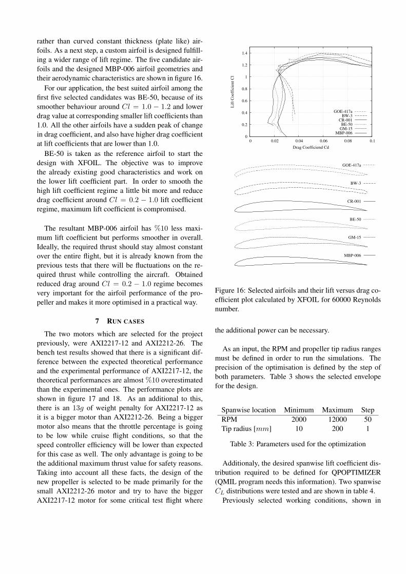
rather than curved constant thickness (plate like) air-

foils. As a next step, a custom airfoil is designed fulfill-

ing a wider range of lift regime. The five candidate air-

foils and the designed MBP-006 airfoil geometries and

their aerodynamic characteristics are shown in figure 16.

For our application, the best suited airfoil among the

first five selected candidates was BE-50, because of its

smoother behaviour around Cl = 1.0 − 1.2 and lower

drag value at corresponding smaller lift coefficients than

1.0. All the other airfoils have a sudden peak of change

in drag coefficient, and also have higher drag coefficient

at lift coefficients that are lower than 1.0.

BE-50 is taken as the reference airfoil to start the

design with XFOIL. The objective was to improve

the already existing good characteristics and work on

the lower lift coefficient part. In order to smooth the

high lift coefficient regime a little bit more and reduce

drag coefficient around Cl = 0.2 − 1.0 lift coefficient

regime, maximum lift coefficient is compromised.

The resultant MBP-006 airfoil has %10 less maxi-

mum lift coefficient but performs smoother in overall.

Ideally, the required thrust should stay almost constant

over the entire flight, but it is already known from the

previous tests that there will be fluctuations on the re-

quired thrust while controlling the aircraft. Obtained

reduced drag around Cl = 0.2 − 1.0 regime becomes

very important for the airfoil performance of the pro-

peller and makes it more optimised in a practical way.

7 RUN CASES

The two motors which are selected for the project

previously, were AXI2217-12 and AXI2212-26. The

bench test results showed that there is a significant dif-

ference between the expected theoretical performance

and the experimental performance of AXI2217-12, the

theoretical performances are almost %10 overestimated

than the experimental ones. The performance plots are

shown in figure 17 and 18. As an additional to this,

there is an 13g of weight penalty for AXI2217-12 as

it is a bigger motor than AXI2212-26. Being a bigger

motor also means that the throttle percentage is going

to be low while cruise flight conditions, so that the

speed controller efficiency will be lower than expected

for this case as well. The only advantage is going to be

the additional maximum thrust value for safety reasons.

Taking into account all these facts, the design of the

new propeller is selected to be made primarily for the

small AXI2212-26 motor and try to have the bigger

AXI2217-12 motor for some critical test flight where

MBP-006

GM-15

BE-50

CR-001

BW-3

GOE-417a

0

0.2

0.4

0.6

0.8

1

1.2

1.4

0 0.02 0.04 0.06 0.08 0.1

Lif

t C

oef

fici

ent

Cl

Drag Coefficiend Cd

GOE-417aBW-3

CR-001BE-50

GM-15MBP-006

Figure 16: Selected airfoils and their lift versus drag co-

efficient plot calculated by XFOIL for 60000 Reynolds

number.

the additional power can be necessary.

As an input, the RPM and propeller tip radius ranges

must be defined in order to run the simulations. The

precision of the optimisation is defined by the step of

both parameters. Table 3 shows the selected envelope

for the design.

Spanwise location Minimum Maximum Step

RPM 2000 12000 50

Tip radius [mm] 10 200 1

Table 3: Parameters used for the optimization

Additionaly, the desired spanwise lift coefficient dis-

tribution required to be defined for QPOPTIMIZER

(QMIL program needs this information). Two spanwise

CL distributions were tested and are shown in table 4.

Previously selected working conditions, shown in

Figure 17: AXI 2217-12 theoretical and experimental

mechanical efficiency curves versus rotation rate for var-

ious input voltages, showing the significant difference

between the theoretical and experimental test results.

Figure 18: AXI 2217-12 theoretical and experimental

shaft torque curves versus rotation rate for various input

voltages, showing the significant difference between the

theoretical and experimental test results.

table 2, used for every run case. As a common result in

every run case, the higher CL distribution gave better

performances. The table 5 shows the best results of all

the run cases. CL1 distribution is selected to be used

for the final design.

The resultant global efficiency is higher using the

bigger AXI2217-12 motor as expected. As it is already

known that the AXI2217-12 is over estimated for the

efficiency and also heavier, the small AXI2212-26

motor fits more appropriately for our application.

A monoblade propeller was also designed using the

same approach. Demanding the same thrust with only

one blade created a propeller with wider chords. This

improved the overall airfoil efficiencies along the span

because of increased Reynolds number. The best esti-

mated overall efficiency for the motor and monoblade

Spanwise location 0.10 0.50 1.00

CL distribution 1 0.75 0.65 0.40

CL distribution 2 0.60 0.45 0.40

Table 4: Lift coefficients distributions

Cruise efficiency RPM Tip radius

[cm]

AXI2212-26 CL1 59.5% 5800 11

AXI2212-26 CL2 58.9% 5700 11.5

AXI2217-12 CL1 63% 5000 12.5

AXI2217-12 CL2 61.9% 5000 12

Table 5: Best global efficiencies of the motor and pro-

peller couples for the cruise conditions are shown (note

that the speed controller losses are not included).

propeller couple is calculated as 62.6% by QPOPTI-

MIZER. Unfortunately, because of the limited time span

of the project and the expected possible problems that

could come with a monoblade propeller cancelled the

investigation of the monoblade concept and the manu-

facturing continued with the bi-blade propeller design.

8 MANUFACTURING

The manufacturing of the propeller is decided to be

done in house, in composite laboratory of ISAE. Think-

ing about each landing phase of the tests flights and hav-

ing no landing gear on the SPOC plane, the propeller

was in danger of breaking while landing. In order to

prevent this, the hub of the propeller is designed for a

folding root, and finally a custom spinner is also build

in the exact needs of SPOC plane. Figure 19 shows the

integration of the folding blade with the spinner.

Figure 19: Designed propeller and its spinner’s CATIA

drawing.

Moulds are designed in Catia V5 and manufactured

with CNC milling machines in order to achieve the nec-

essary precision. Each blade is build out of three piece

of moulds, top, bottom and the folding axis pin. The

spinner cone is build by using six pieces of moulds, two

sides, two folding axe pins and two prop blade root in-

serts. Finally the base of the cone is build by using three

moulds, top bottom and the rotation axis pin. The spin-

ner cone and the base moulds are designed to fit each

other in order to maintain the base to the cone in the

same rotation axis perfectly to prevent any possible bal-

ance problems.

The propeller was made of carbon fibre. The material

was chosen because of its low weigh and its high

strength. The required pieces are first cut into shape

and then wet lay-up is done by hand into the moulds.

Different orientations (45 and 90) of carbon fibre

woven were used on the skin for the torsional strength

of the propeller. Additionally, unidirectional carbon

fibre mesh were placed in order to sustain the bending

forces of the blade. As the propeller blade has a specific

airfoil, a certain amount of material should have filled

the thickness. The exact required material quantity is

found by trial and error as the weight of each blade was

only 1.5 g. There was no need to use vacuum bagging

process as the two mould halves completely fits onto

each other.

The spinner cone is also build by wet lay-up by hand,

in order to achieve a smooth surface and fix the layer

on the skin of the cone, a balloon is inflated inside the

cone. A silicon insert should have given better results

but this method is used because of the time restrictions.

The figure 20 shows the resulting cone and its molds.

Figure 20: The cone and its molds

Finally after manufacturing two blades, spinner cone

and the base, they are integrated into each other to form

the custom designed propeller. The figure 21 shows

the resulting propeller. The fixation of the spinner to

the motor shaft is done internally. First the two blades

should have removed and then the inner fixation screws

that are placed on the spinner base plate can be reached.

This method makes the fixation a little bit complex but

once it is fixed there will not be any gap between the

spinner and the nose of the plane or any protruding

screws that can create additional drag.

Figure 21: The resulting custom propeller

9 TEST RESULTS

The propeller test bench which is shown in section 4.3

figure 14 is used for the tests. The main point of inter-

est was to measure the performance at cruise conditions

which are 15 m/s of flight speed and 1.3 N of thrust

generation. Additionally, as expected from the theoreti-

cal calculations, the propeller has to have more than 4 Nof thrust at this flight speed at full throttle. Figures 22

and 23 show the global efficiency (speed controller +

motor + propeller) and propeller efficiency alone versus

thrust generated at 15 m/s flight speed condition. It can

be seen that the propeller efficiency is around 71% at

cruise condition thrust, and the final global efficiency is

around 50% which includes the speed controller, motor

and the propeller. The maximum thrust measured at full

throttle was 4.25 N at 15 m/s speed.

Expected global efficiency was 59.5% however, the

measured efficiency was only 50%. The assumptions

and the simplifications that is done in theoretical calcu-

lations will cause a difference between the real world

and the calculations, but there are also several reasons

that cause difference. First of all the theoretically

assumed 59.5% efficiency does not take into account

the speed controller, which usually have around 95%of maximum efficiency. Additionally, the designed

spinner could not have used in the wind tunnel tests

because of the additional pressure drag that it generates

without having the real fuselage behind it. Instead of

spinner, an aluminium piece is manufactured in order

to hold the two folding propeller blades together in

the wind tunnel, there is additional drag coming from

this piece resulting with lower efficiency. Finally the

manufactured airfoil shape and the propeller geometry

could have differ from the designed and analysed

one which results normally reduction on the expected

efficiency as well.

0 0.5 1 1.5 2 2.5 3 3.5 40.2

0.25

0.3

0.35

0.4

0.45

0.5

0.55Custom Propeller at V=15 m/s

Thrust [N]

Glo

bal E

ffic

iency [

]

Figure 22: The global efficiency versus Thrust [N] plot

for the custom designed propeller at 15 m/s speed.

0 0.5 1 1.5 2 2.5 3 3.5 4

0.35

0.4

0.45

0.5

0.55

0.6

0.65

0.7

0.75

0.8Custom Propeller at V=15 m/s

Thrust [N]

Pro

pelle

r E

ffic

iency [

]

Figure 23: The propeller efficiency versus Thrust [N]

plot for the custom designed propeller at 15 m/s speed.

10 CONCLUSION

A multi-point optimisation methodology and a de-

voted program called QPOPTIMIZER is introduced for

matching and designing electric propulsion system. The

importance of the mission definition and optimisation

of the propulsion system according to multiple working

conditions is highlighted. The modelling of the motor

and propeller is described stating the importance of the

accuracy of the models. The motor and propeller match-

ing procedure is explained deeply.

Finally, the proposed program is used in designing a

custom propeller for a real life application for a mini-

UAV that has to fly a long range mission. The results

showed that the program correctly matches the motor

and propeller’s individual peak efficiency regions opti-

mised while taking into account every working condi-

tions. This leads to an optimum selection of the propul-

sion system. However, the resultant performance val-

ues are a little bit optimistic (%5 − 10 for the complete

propulsion system) compared to the experimental mea-

surements which has been previously expected.

ACKNOWLEDGEMENT

The authors would like to thank Prof. Mark Drela

for sharing his great work QPROP and QMIL within the

GNU v2 licence which makes it possible to use them as

the core aerodynamic analyser programs of the QPOP-

TIMIZER. Also we would like to thank a lot Xavier

Foulquier and Guy Mirabel for their precious helps and

advices for the composite manufacturing.

The realisation of the custom propeller would not be

possible without the work that has been done by Miguel

Morere Y Van Begin, Guillaume Soete, Pierre Joachim

and Benjamin Fragniere(aka. The Belgium Beatles). Fi-

nally, this study has been co-funded by the European

Union. Europe is involved in Midi-Pyrenee with Euro-

pean Fund for regional development.

REFERENCES

[1] Thomas J. Mueller, James C. Kellogg, Peter G.

Ifju, and Sergey V. Shkarayev. Introduction to the

Design of Fixed-Wing Micro Air Vehicles. Ameri-

can Institute of Aeronautics and Astronautics,Inc.,

Virginia,VA, 2007.

[2] Murat Bronz, Jean-Marc Moschetta, Pascal Bris-

set, and Michel Gorraz. Towards a Long En-

durance MAV. In EMAV2009, Delft, Netherlands,

September 2009.

[3] Murat Bronz, Jean-Marc Moschetta, Pascal Bris-

set, and Michel Gorraz. Towards a Long En-

durance MAV. International Journal of Micro Air

Vehicles, 1(4):241–254, 2009.

[4] Murat Bronz, Jean-Marc Moschetta, and Pascal

Brisset. Flying Autonomously to Corsica : A Long

Endurance Mini-UAV System. In IMAV2010,

Braunschweig, Germany, July 2010.

[5] Mark Drela. QPROP Formulation. MIT Aero and

Astro, June 2006.

[6] A.Betz. Airscrews with minimum energy loss.

Technical report, Kaiser Wilhelm Institute of Flow

Research, 1919.

[7] S.Goldstein. On the vortex theory of screw pro-

pellers. In Proceedings of the Royal Society, vol-

ume 123, 1929.

[8] Theodore Theodorsen. Theory of Propellers.

McGraw-Hill, New York, 1948.

[9] E.E Larrabee and S.E. French. Minimum induced

loss windmills and propellers. Journal of Wind En-

gineering and Industrial Aerodynamics, 15:317-

327:317–327, 1983.

[10] Mark Drela. First-order dc electric motor model.

Technical report, MIT, Aero and Astro, February

2007.

[11] Mark Drela. Dc motor and propeller matching ,

lab 5 lecture notes. Technical report, MIT, March

2005.

[12] McCormick B.W. Aerodynamics, Aeronautics &

Flight Mechanics. John Wiley & Sons, Inc., 1979.

[13] Michael Selig. Summary of Low-Speed Airfoil

Data, volume 1. SoarTech Publications, Virginia

Beach, VA, 1995.

[14] Michael Selig. Summary of Low-Speed Airfoil

Data, volume 2. SoarTech Publications, Virginia

Beach, VA, 1996.

[15] Michael Selig. Summary of Low-Speed Airfoil

Data, volume 3. SoarTech Publications, Virginia

Beach, VA, 1997.