MULTI-PHYSICS MODELLING AND SIMULATION: … 2006 - Keynote.pdf · ANSYS/Multi-physics ... -single database & memory map so that no data transfer & efficient memory use ... use the

Multi-Physics 2006, MariborDecember 2006

MULTI-PHYSICS MODELLING AND SIMULATION:

CHALLENGES AND OPPORTUNITIES

M. Cross, T.N. Croft, D. McBride, A.K. Slone, and A.J. Williams

Centre for Civil and Computational Engineering

School of EngineeringUniversity of Wales, Swansea

[email protected]

mailto:[email protected]

Multi-Physics 2006, Maribor

Why Multi-Physics?

Large number of real-world problems are multi-physics.

Castings ComponentsElectronic Packaging


CAE analysis tools market history

FEA started mid 60’s with NASTRAN, Abaqus, ANSYS, etc as major players

CFD started 1980 with FLUENT,CFX, PHOENICS and STAR-CD as major players

MDA started mid 1990’sCoupling codes MDICE, Spectrum, PHYSICA

1965 008575 95 05

10

10K

1K

100

100K

FEA CFD

MDA

Licenses


Why Multi-physics Modelling ?Large number of real world problems require multi-physics simulation tools.Examples

Solidification problems – Solder JointsFluid-Structure interaction – Flutter in aircraft wings

Need to solve for integrated physicsEnsure two-way coupling

Fluid Flow

Stress Analysis

Electromagnetics

Heat Transfer


Commercial Software – Multi-physics

Number of products claiming to be multi-physicsANSYS/Multi-physics

http://www.ansys.com/PHYSICA

http://www.physica.co.uk/COMSOL

http://www.comsol.com/Algor

http://www.algor.com/DYNA- http://www.lsc.comADINA- http://www.adina.comFlomerics

http://www.flomerics.com/

Airflow Temperature

Stress

http://www.ansys.com/

http://www.physica.co.uk/

http://www.comsol.com/

http://www.algor.com/

http://www.lsc.com/

http://www.adina.com/

http://www.flomerics.com/


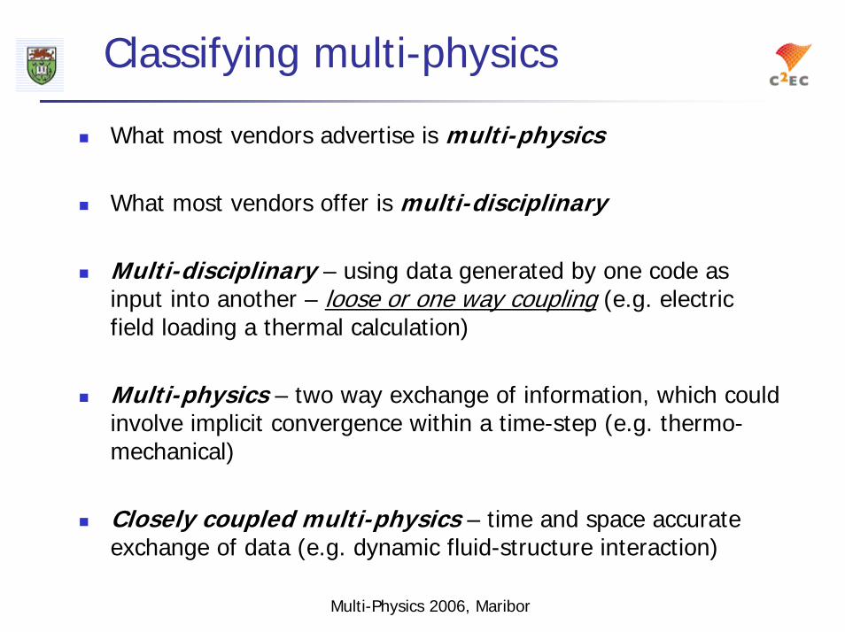
Classifying multi-physics

What most vendors advertise is multi-physics

What most vendors offer is multi-disciplinary

Multi-disciplinary – using data generated by one code as input into another – loose or one way coupling (e.g. electric field loading a thermal calculation)

Multi-physics – two way exchange of information, which could involve implicit convergence within a time-step (e.g. thermo-mechanical)

Closely coupled multi-physics – time and space accurate exchange of data (e.g. dynamic fluid-structure interaction)


MDA vs. MULTI-PHYSICSMust distinguish between MDA and multi-physics:

one loosely coupled, other tightly coupledone significant challenge, other major new technology development

Multi-physics analysis always involves challenging flow analysis, so must be designed to compete well with leading edge CFD tools

Limited CFD => limited multi-physics

Limited parallel scalability => limited multi-physics

Fluid Flow Stress

Heat Transfer Electromagnetics

Fluid Flow Stress

Heat Transfer Electromagnetics


Multi-physics Modelling

Physics RequirementsFluid FlowHeat transferSolidification/phase changeStressElectro-magnetics

Geometry Complex

Large simulations

MULTI-PHYSICS

UNSTRUCTURED

PARALLEL

Key issue: CFD capability


Simulation technologies

Key players for thermo-fluid based models:- CFX - FLUENT- STAR-CDKey players for thermo-mechanical models:- ANSYS- ABAQUS- NASTRANKey player for electro-magnetics:- OPERA & CONCERTO, Vector fields


Computational approaches

Most ‘leading’ CFD codes use FV methods on unstructured meshAll CSM codes based upon FE methods with a wide variety of element typesCEM usually based on FE (and sometimes BE) methodsHandling the physics interaction –the challenge!


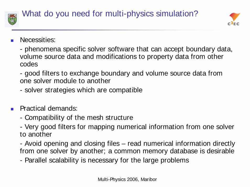
What do you need for multi-physics simulation?

Necessities:- phenomena specific solver software that can accept boundary data, volume source data and modifications to property data from othercodes- good filters to exchange boundary and volume source data from one solver module to another- solver strategies which are compatible

Practical demands:- Compatibility of the mesh structure- Very good filters for mapping numerical information from one solver to another- Avoid opening and closing files – read numerical information directly from one solver by another; a common memory database is desirable - Parallel scalability is necessary for the large problems


Key issues in closely coupled multi-physics simulation

Phys-A Phys-B

• Good numerical filters to map data from one solver into another

•Interpolation from one setof variables to another =>compatibility of mesh

• Single database of mesh data & simulation variables

• Solver strategy- Direct vs Iterative- Eulerian vs Lagrangian

•Is coupling strategy compatiblewith scalable parallelism, EVEN if software components are parallel?

Practicalities of multi-physics simulation


MpCCI – a tool for code interoperability

Coupled physics implies coupling of separate phenomena codes:- without opening/closing files- operate in a parallel contextEmerged from an EU project – public domain OPEN SOURCE toolswww.scai.fraunhofer.de/mpcci.0.htmlApplications to fluid-structure interaction:- ABAQUS + FLUENT for DFSI- STAR-CD + NASTRAN for DFSIBUT exchanging data does NOT necessarily mean coupling of the physics that is time or space accurate

http://www.scai.fraunhofer.de/mpcci.0.html


Key route to closely coupled multi-disciplinary (multi-physics) simulationBasic requirements of a SSF:- consistency of mesh for all phenomena- compatibility in the solution approaches to each of the phenomena

- single database & memory map so that nodata transfer & efficient memory usebetween programs

- facility to enable accurate exchange ofboundary or volume sources (e.g. body force)

- enables scalable parallel operation for all physics interactions

Alternative approach:Single Software Framework


Attempts at SSF for multi-physics

COMSOL – FEMLAB- Originally based on MATLAB as a suite of FE discretisation routinesOEFELE – Open Engineering- An FE based solver frameworkFOAM- solver framework for FE and FV discretisationsPHYSICA- FV based tools for multi-physics


PHYSICA – Multi-physics Framework

- Work started in late 1980s at University of Greenwich- Based upon FV methods on unstructured mesh (FV-UM)- Conservative approach:

**FV-UM discretisation used for everything**- Flow/ electro-magnetics/ heat transfer procedures from FV-SM -> FV-UM - Solid mechanics developed from scratch - Prototypes moved from:

a) 2 ->3D and b) scalar -> parallel

- Key issue was to ensure FLOW worked well in all contexts- Solidification processes a key target


Spatial Discretisation in PHYSICA

Vertex Based

MeshElement

GaussPoint

Finite VolumeCell Centred

ControlVolume

ControlVolume

Integration Point

x

Finite Element

x

Node

Finite Volume

x

x

x

x

x

xx

xxx

x

Unstructured meshCSM

Vertex basedFV

CFDCell centredFV


Finite Volume Method

Domain divided into a number of finite size control volumes (CV)Conservation equation integrated over each CV and timeApproximations to each term yields a linear system in the unknown values of the variable φ,

( ) ( ) ( ) φφρφρφ St

+∇Γ⋅∇=⋅∇+∂

∂ u


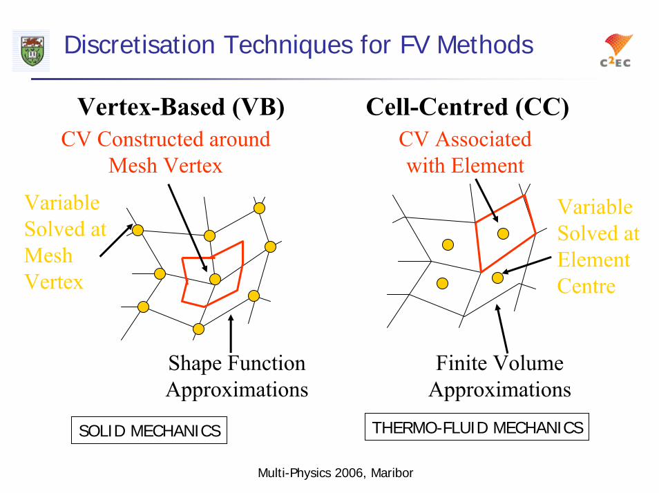
Discretisation Techniques for FV Methods

Vertex-Based (VB)CV Constructed around

Mesh Vertex

Variable Solved at Mesh Vertex

Shape Function Approximations

Cell-Centred (CC)CV Associated with Element

Variable Solved at Element Centre

Finite Volume Approximations

THERMO-FLUID MECHANICSSOLID MECHANICS


Continuous casting process: example of CFD based multi-physics

B.G. Thomas

Mixture of liquid steel and argon injected into rectangular mould

Liquid metal flux sits on top of mould

Water cooled mould extracts energy forming a solid steel shell

Continuous withdrawal


Multi-phase equations

Mass and momentum

Energy

Density

( ) ( ) ( )

( ) 0)(ln

.

=⋅∇+

+∇−∇∇=⋅∇+

u

Suuuu

tDD

pt

ρ

µρρ∂∂

( ) ( ) ( ) hTkhht

Su +∇∇=⋅∇+ .ρρ∂∂

fluxgasmetal or ( ρρφφρρ == ),


Free surface (SEA)Solves:

where φ is the fraction of metal in a cell

van Leer scheme used to reduce smearing of interfacecontinuity equation solved for volume not massproperties a linear combination of phases present

0. =∇+∂∂ φφ u

t


Solidification

Release of energy due to phase change

Darcy source for momentum equations

( ) ( )

⎪⎪⎩

⎪⎪⎨

⎧

<

≤≤⎟⎟⎠

⎞⎜⎜⎝

⎛−−

>

=

⋅∇−∂∂

−=

tempsolidustheTT

zonemushytheinTTTTTTT

templiquidustheTT

f

LfLft

S

S

LSSL

S

L

L

LmLmh

, 0

,

, 1

uφρφρ


Argon Bubbles

CFD - a mixed Lagrangian – Eulerian calculation:calculate the flow field using CFD procedureuse the flow field to influence the particle movement

B/D/P equations (Argon bubbles in this case) are solved explicitly in Lagrangian framework.New position of each particle at given time-step computed from the particle equation of motion. Particle is subjected to a drag force Cd and buoyancy but no turbulence feedback.Drag force is an empirical function of the "slip" Reynolds number between particle and surrounding fluid. Account is taken of

the particles entering and leaving each computational cell the time taken between entry and exit.

Giving the instantaneous volume fraction of Argon in each cell, which is used to adjust the average density or other cell properties


Argon bubble injection:closely coupled L-E approach

Evalintegrated

path

L particlesEmbed withmass flux

effects

Incorp in contCFD code


Solution domain


z

Solid regions appear in blue

EndView

Top view

Solidification Strand


Clustering of argon bubbles

Solved using PHYSICA


Coupled EM-flow calculations

For most practical calculations in metals processing:The EM field influences the flow and thermal fieldsBUT the thermo-fluid phenomena has little influence of the EM fieldsHence, essentially one way coupling So calculate the EM field and calculate the thermal and flow loads in the CFD calculation


Example: Electromagnetic brake simulations

Computations were also performed to estimate the effects of EMB on the free surface . For this the Maxwell equations were solved, which with the usual MHD assumptions, lead to:

0 = B.∇Continuity of magnetic flux:

Ohm's Law for conducting metals φσ ∇× - = E where),BU + E( = J

µσηη

m

2 1 = where,B + )BU( = t

∇××∇∂∂BMagnetic Transport, or

Induction equation

BJFL ×=Lorentz force:

Note: Terms containing the velocity U, are only important when Rm (=LU/η)> 1


Brake arrangement

S N

Two electromagnets of opposite polarity (By=±0.4T ) placed in the jet region to reduce velocity and hence, surface deformation


Fluid behaviour under EMB conditions

Flow suppressedhere

B=0.4T B=0T


Welding processes simulation -natural multi-physics

Processes involve:— free surface flow— electromagnetic forces— heat transfer with solidification/melting— development of non-linear stress

Ideal candidate for multi-physics modelling


T-Junction arc weld simulation


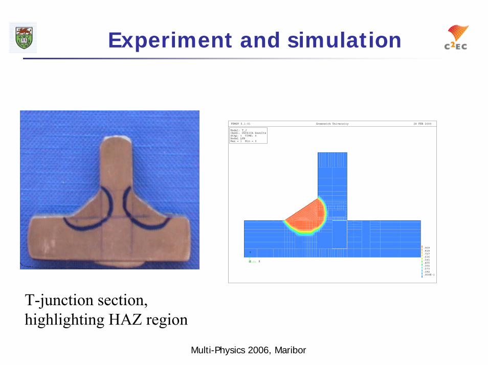
Experiment and simulation

X

Y

Z

Model: T_JCASE1: PHYSICA ResultsStep: 1 TIME: 0Nodal LFNMax = 1 Min = 0

.909E-1

.182

.273

.364

.455

.545

.636

.727

.818

.909

FEMGV 5.1-01 28 FEB 2000Greenwich University

T-junction section, highlighting HAZ region


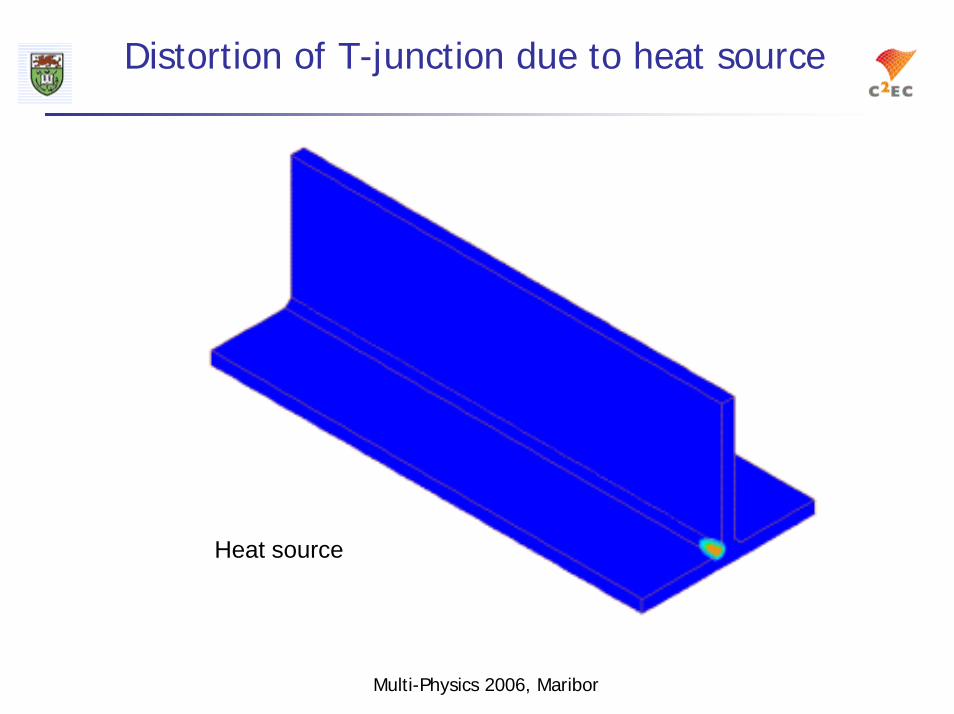
Distortion of T-junction due to heat source

Heat source


Weld pool dynamics

Velocity vectors in crossectionLorentz force distribution in the weld-pool


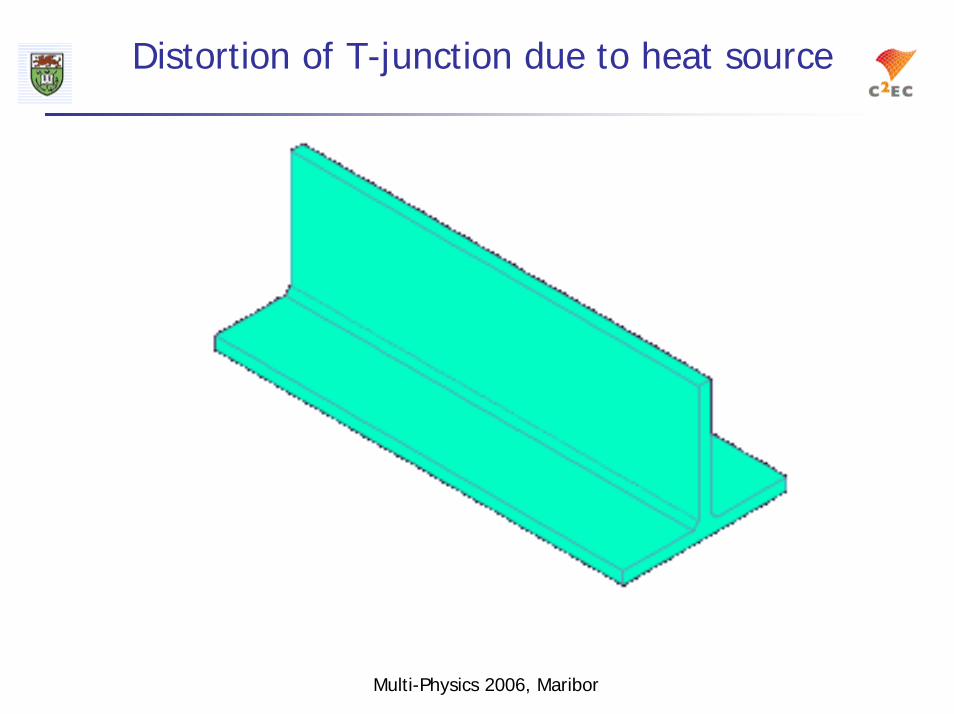
Distortion of T-junction due to heat source

Distortion


Welding – multi-physics BUT . .

Welding involves:- free surface fluid flowheat transfer and solidification/melting- electro-magnetic fields- non-linear stress

BUT . . no coupling back:- from thermo-fluids to EM field- from stress calculation to thermo-fluids

SO . . reasonably loosely coupled


Generic Dynamic Fluid Structure Interaction

Closely coupled multi-disciplinary problemTime & space accurateVery challenging in every respect.Issue of GCL

Implementation of boundary conditions.

Features of single software framework:Consistency of mesh.Single database & memory map.Compatibility in the solution approaches FV-UM.

Traction boundary condition

CFD CSM

DeformationMeshadaptation


Three Phase Approach

CMD

1+⇒ nn tt

mmm FdK =CSD

( )tsFKddCdM =++ &&&

fsm Γon u

fsfsp Γ= on σt

fsΓon d

Generalised Newtonian Continuity

CFD


Spatial Discretisation for closely coupled multi-physics

Vertex Based

MeshElement

GaussPoint

Finite VolumeCell Centred

ControlVolume

ControlVolume

Integration Point

x

Finite Element

x

Node

Finite Volume

x

x

x

x

x

xx

xxx

x

Unstructured mesh

CFDCell centredOr mixed CC- VBFV

CSMVertex basedFV/FE


Structural Dynamics

Equilibrium Equation

Method of Weighted ResidualsGreens 1st theorem

where evaluated at nodes

( ) 02

2

=−+ dbLt

dtdρσ

jjdN ˆ≈d

( )

( ) Γ−Ω+Γ+Ω=

Γ−Ω+Ω

∫∫∫∫

∫∫∫

ΓΩΓΩ

ΓΩΩ

ddd

dd

TT0

T2

2

idit

d

i

T

ipiT

i

jij

T

ijT

i

dt

dNddNdt

ddN

00 TWLWWbW

TDLWDLLWW

σσ

ρ


Dynamic Structural Mechanics

Compact matrix form of equilibrium equation

where C is the damping matrix

traction boundary condition on fluid – structure boundary

( ) ( ) fdKdCdM =++ ˆˆdtdˆ

dtd

2

2

( )

( ) Γ−Ω+Γ+Ω=

Γ−Ω=

Ω=

∫∫∫∫

∫∫

∫

ΓΩ

ΓΩ

ΓΩ

Ω

dddd

dNdN

dN

idi

idi

idi

i

Ti

Tip

Ti

T

jT

ijT

iij

jTiij

000 TσWσLWtWbWf

TDLWDLLWK

WM

i

ρ

sijj

ijp xu

pt Γ⋅∇⎟⎟⎠

⎞⎜⎜⎝

⎛

∂

∂+

∂∂

+−= on - xu 3

2i δµµδ uij


CSM Spatial Formulation

Essential difference between FE & FV Weighting Functions

FE FVdirect association between within cvNi & element zero elsewhere

Mass matrixFE

FV

ii N=W IW =i

∫

∫

Ω

Ω

Ω=

Ω=

i

i

jij

jT

iij

N

NN

d

d

ρ

ρ

M

M


CSM Spatial Formulation

Stiffness matrixFE

FV

Load vectorFE

FV

( ) Ω= ∫Ω

dNN j

T

jij

i

DLLK

( ) Ω+Γ+Ω= ∫∫∫ΩΓΩ

dd T0 0Lbf σ

T

ipiT

i NdtNNit

Γ−Γ+Ω= ∫∫∫ΓΓΩ

dd0

idit

dt p 0Tbf σ

∫Γ

Γ−=i

djij NTDLK


Comparison of FE and FV performance

3D cantilever

L = 20m , b = d = 2mν = 0.2, ρ = 2600 kg m-3 , E = 10 GPaF = 2000 N

Mesh 80x8x85120 elements and 6561 nodes

Analytic 2d solution Fenner ν = 0

F

Fixed Free

db

L


Comparison of FE and FV performance

3D cantilever, static results on Dec Alpha 466 MHz processor

Iterations Run times, second

ν FE JCG

0.3 539 540 544 48 95 98

483

438

FE-BICG FV-BICG FE JCG FE-BICG FV-BICG

0.2 483

438

44 85 88

0.0

483

437 38 78 80


Cantilever Dynamic Displacement


Fluid velocity & pressure fields

Re 4000


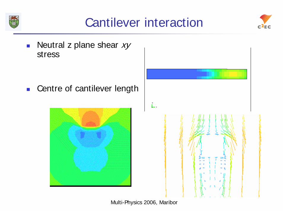
Cantilever interaction

Neutral z plane shear xystress

Centre of cantilever length


Dynamic fluid-structure interaction

Wind directionFlow induced vibrations

Targeted at problems involving flow induced vibrations

Use dynamic structural equations and Navier-Stokes flow equationsObjective: move to VB flow and FE based dynamics


Dynamic response of structure without flow


Fluid Velocity and Pressure Movies

At tip of wing


Shear Stress σxy Movie

Multi-Physics 2006, MariborDecember 2006

Parallel Multi-Physics Modelling


Multi-physics compute demands: secs per node(elt)/time step per problem class

Unstructured Mesh analysis = 3* Structured mesh analysisPerformance on a Compaq alpha 466Mhz- Heat Transfer (HT) + Solidification (Sol) = 2. 10-3- Fluid Flow (FF) + HT + Sol = 6.10-3- HT + Sol + Stress = .09- FF + HT + Sol + Stress = .14

=> a casting simulation with 100K nodes, and 100 time steps is 300+hrs!We need simulation times 100x faster

PARALLEL – WITH CHANGING PHYSICS


Parallel Strategy -PHYSICA

Single Program Multiple Data (SPMD)

Program resident on each processorMesh Partitioned across processors.Minimise communication times.


Parallel Multi-Physics Framework

Simulations very Time Consuming – need Parallel capability

CAPlib JOSTLE

PHYSICAPDE Solver

Generic Parallel Calls Lib Mesh Partition


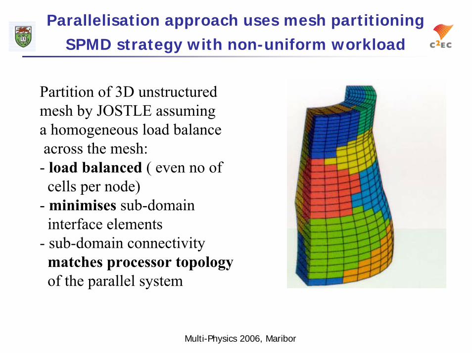
Parallelisation approach uses mesh partitioning SPMD strategy with non-uniform workload

Partition of 3D unstructuredmesh by JOSTLE assuminga homogeneous load balanceacross the mesh:- load balanced ( even no of cells per node)

- minimises sub-domain interface elements

- sub-domain connectivitymatches processor topologyof the parallel system


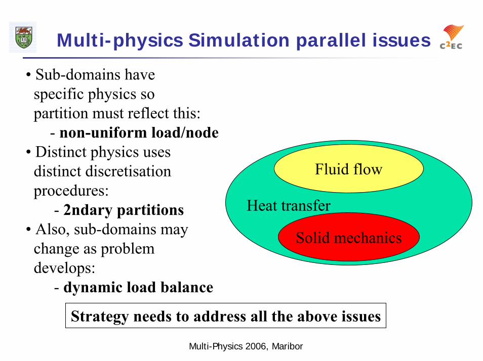
Multi-physics Simulation parallel issues

Solid mechanics

Fluid flow

Heat transfer

• Sub-domains havespecific physics sopartition must reflect this:

- non-uniform load/node• Distinct physics uses distinct discretisationprocedures:

- 2ndary partitions• Also, sub-domains may change as problem develops:

- dynamic load balance

Strategy needs to address all the above issues


Primary & secondary partitions

Primary & secondarymeshes

Good primary & poorSecondary partition

Good primary &Secondary partitionsfrom JOSTLE


Parallel multi-physics: two level approach

Implement a generic parallel version of Multi-physics code/ MDA codes

- without regard to in-homogeneity of the computational work over the mesh(es) defining the analysis domain

Dump the load balancing into the mesh (re)partitioning task -JOSTLE_DLBProcess as straightforward as possible

JOSTLE

PHYSICAPDE Solver

Mesh Partition


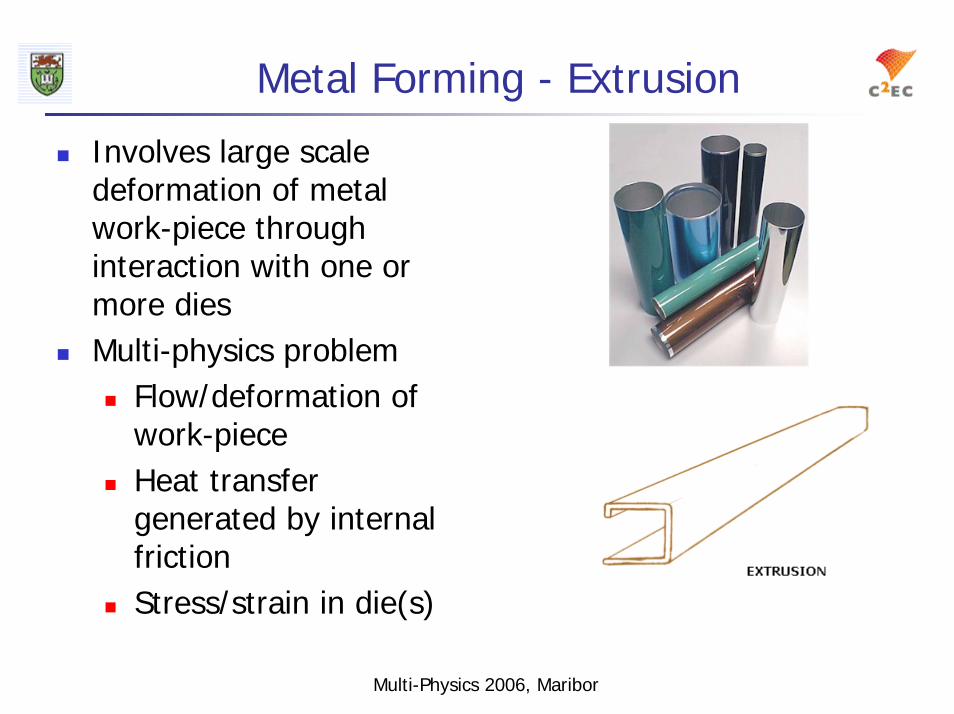
Metal Forming - Extrusion

Involves large scale deformation of metal work-piece through interaction with one or more diesMulti-physics problem

Flow/deformation of work-pieceHeat transfer generated by internal friction Stress/strain in die(s)


Mixed Eulerian-Lagrangian Approach

WorkpieceEulerian mesh

Free-surface algorithm to track deformation

Non-Newtonian material model

Heat transfer plus energy generated by internal friction

DieLagrangian mesh

Mechanical behaviour coupled with:

Thermal behaviour in workpiece

Fluid traction load from workpiece


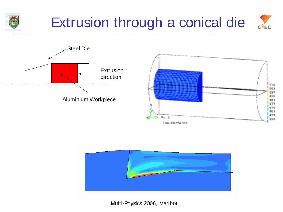
Extrusion through a conical die

Extrusion direction

Steel Die

Aluminium Workpiece


Governing Equations - Extrusion

Coupled Thermo - mechanical problemHeat transfer significant factor in deformation process

CFDNon-Newtonian viscosity model – Plastic Norton Hoff lawHeat Transfer - Friction between die and workpiece.Free Surface - Van Leer method

CSMStatic equilibrium equation – linear elastic solid.

Coupling at the workpiece/die boundary:Die subject to fluid traction boundary condition.Workpiece subject to a die velocity boundary condition.Dynamic meshes – GCL. Fluid velocity relative to mesh movement.


Governing EquationsFree Surface

Scalar Equation Method ~ marker φ used to track free surface

Advection Scheme - Van-Leer

∆φ/∆n dependant on value of φ for upwind-upwind elementDensity Gradients – GALA algorithm

Coupled thermo-mechanical problem Heat transfer significant factor in deformation process.Energy entered into thermal equation as:

Temperature development dependant on energy dissipation at rate:

β is proportion of plastic deformation energy dissipated as heat in solid material.

( ) 0=⋅∇+∂∂ φφ u

t

( )( )tdn faceuduface ∆⋅−

∆∆

+= ||21 nuφφφ

( ) ( ) ( ) rTkTcTct pp &+∇⋅∇=⋅∇+

∂∂ uρρ

ijijijr εβσ && =


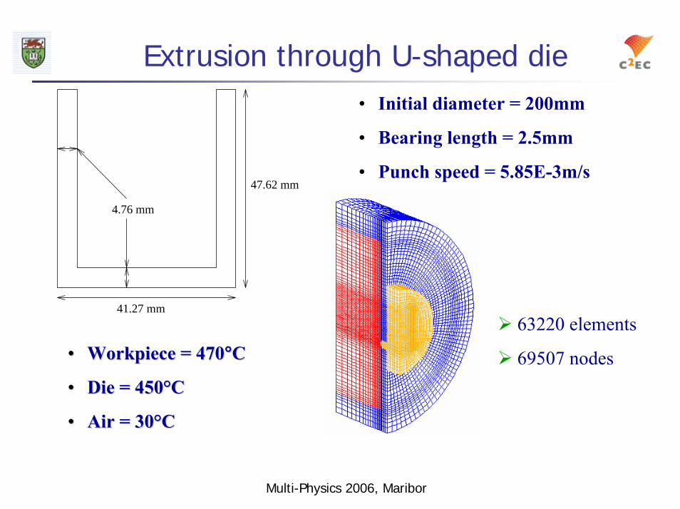
Extrusion through U-shaped die

4.76 mm

41.27 mm

47.62 mm

• Initial diameter = 200mm

• Bearing length = 2.5mm

• Punch speed = 5.85E-3m/s

63220 elements

69507 nodes•• Workpiece = 470Workpiece = 470°°CC

•• Die =Die = 450450°°CC

•• Air = 30Air = 30°°CC


Temperature contours in extruding work-piece


Effective stress contours and deformation of die


Parallel results

ProcessorsRun time(hours)

Speed-up

1 81.9 14 18.3 4.488 10.2 8.0312 7.5 10.9216 6.1 13.43 Single phase mesh partitions on 16 processors

Itanium IA 64 cluster running Linux OSEight nodes, two 733MHz processors per nodeEach node with 2 Gb memory & 2Gb swap space


Finite Volume Methods for CFD: CC

Strengths and weaknesses:

Cell centred methods:memory efficientfast

BUTaccuracy fades rapidly as mesh quality degradesfails to converge with poor quality meshescorrection terms help

slows convergencestability

Cell-Centred (CC)CV Associated with Element

Variable Solved at Element Centre

Finite Volume Approximations


FV Methods for CFD: VB assessment

Vertex-Based (VB)CV Constructed around

Mesh Vertex

Variable Solved at Mesh Vertex

Shape Function Approximations

Strengths and weaknesses:

Vertex centred methods:heavy on memoryrelatively compute intensivegood accuracy as mesh quality degradesconverges with almost any kind of mesh, no matter how poor its quality


Concept Of Approach for VB CFD

Solution of Flow Variables

Vertex-Based

All Other CFD Variables

Solved

Cell-Centred

Good Resolution of Flow Field

Enables Solutions on Distorted Meshes

Handles Skewed Meshes

with EaseFast & EfficientComputationally

Expensive

Motivation - physics rich CFD module using CC methods for all transport variables


Increasingly skewed meshes for VB

Beltrami problem – 3D benchmark with analytical solution


Measured numerical errors for VB, CC and combinations


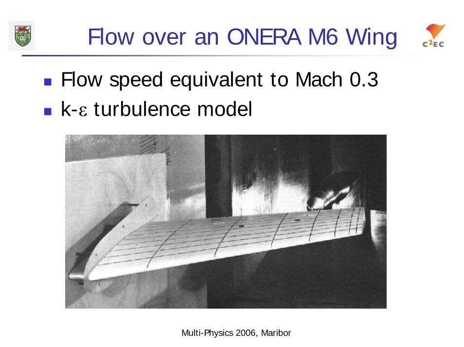
Flow over an ONERA M6 Wing

Flow speed equivalent to Mach 0.3k-ε turbulence model


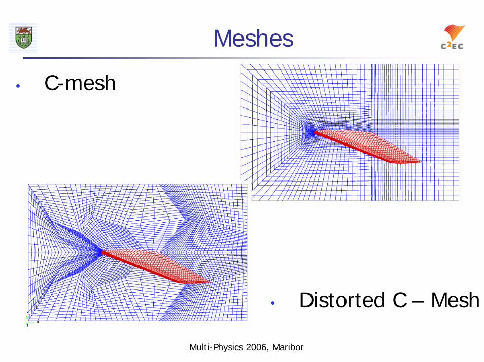
Meshes

• C-mesh

• Distorted C – Mesh


Mesh element quality

Angle: Below 30o : Above 150o


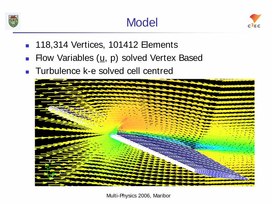
Model

118,314 Vertices, 101412 ElementsFlow Variables (u, p) solved Vertex BasedTurbulence k-e solved cell centred


Results

Mach Number Turbulent Viscosity

a) C-mesh results b) distorted C-mesh results


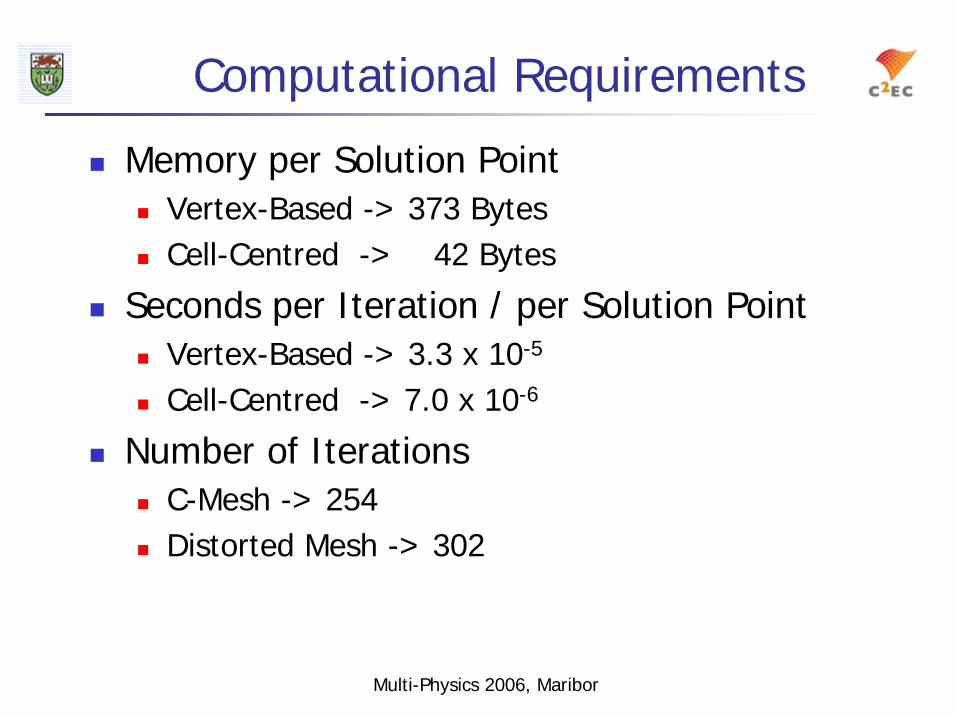
Computational Requirements

Memory per Solution PointVertex-Based -> 373 BytesCell-Centred -> 42 Bytes

Seconds per Iteration / per Solution PointVertex-Based -> 3.3 x 10-5

Cell-Centred -> 7.0 x 10-6

Number of IterationsC-Mesh -> 254 Distorted Mesh -> 302


Example of VB-CC calculation:free surface capture

SEA solves for the whole domain as a two component fluid and tracks the free surface developmentUses D-A and van Leer schemes to sharpen surface captureImplemented using CC discretisationProcedure re-implemented using VB velocity components which are interpolated onto cell faces, and then hooked into conventional SEA


Simple test problem:collapsing liquid column

Liquid

(Φ = 1)

Air

(Φ = 0)

Key issue here is to test free surface procedure as the mesh quality is reduced

Mesh quality – non orthogonality ranges from 7 to 175 deg

CC has no chance of converging – question how does VB-CC method converge & how does accuracy degrade?


Simple test application:2D collapsing column


Comparison with cartesian mesh

Key issues:

• Convergence-Good

• Accuracy degradation- localised


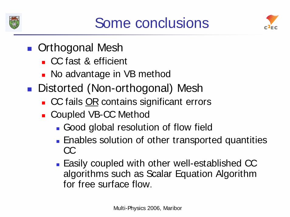
Some conclusions

Orthogonal MeshCC fast & efficientNo advantage in VB method

Distorted (Non-orthogonal) MeshCC fails OR contains significant errorsCoupled VB-CC Method

Good global resolution of flow fieldEnables solution of other transported quantities CCEasily coupled with other well-established CC algorithms such as Scalar Equation Algorithm for free surface flow.


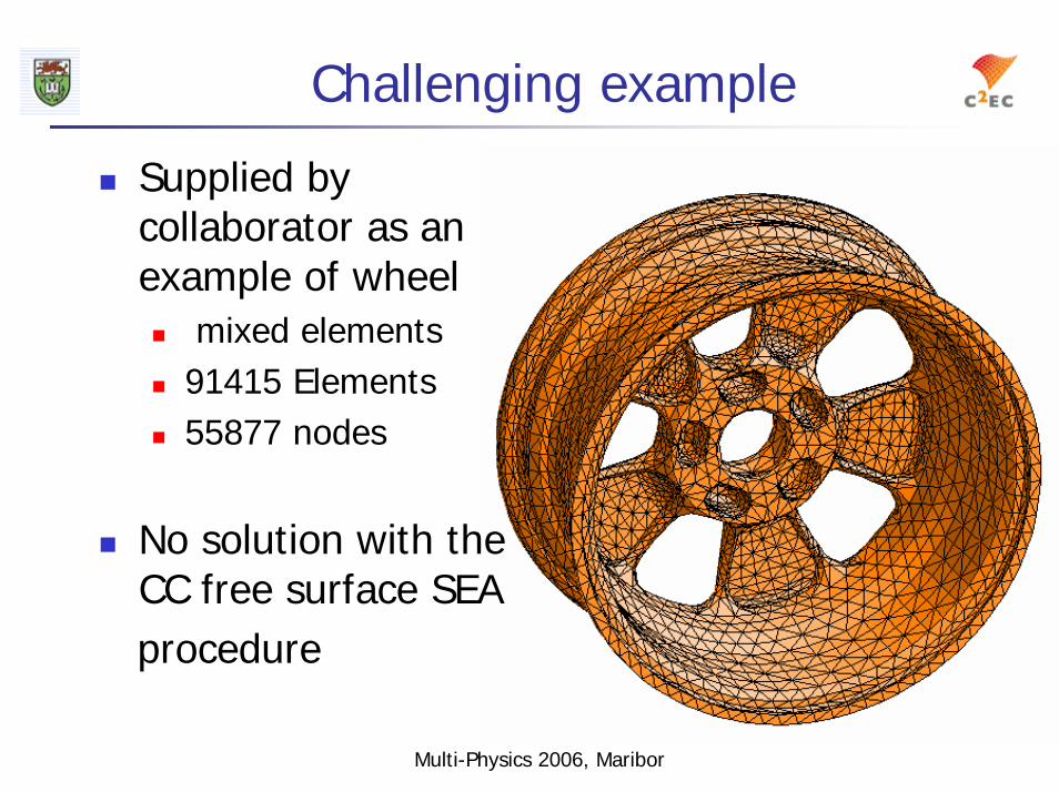
Challenging example

Supplied by collaborator as an example of wheel

mixed elements91415 Elements55877 nodes

No solution with the CC free surface SEA procedure


Application to a real case: the wheel

116.3 mm

207 mm

424 mm

69.8 mm

38.4 mm


Mesh element types and complexity

36296 Pyramids24013 Tetrahedrals11390 Pentahedrals19716 Hexahedrals

• 55877 Vertices

• 91415 Elements


Problems with mesh quality


Boundary conditions & flows

Inlet at Rim

Outlet

Inlet velocity 100 mm/s


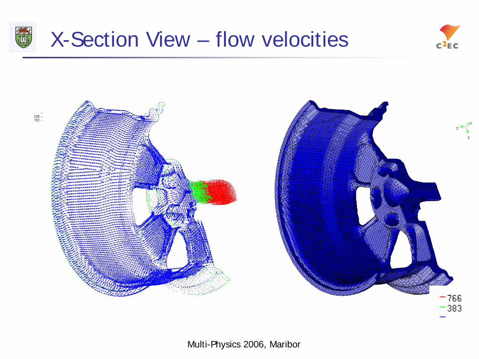
X-Section View – flow velocities


The filling process


Run time data

Velocity is solved using a variant of SIMPLE with outer time stepFree surface marker is tracked explicitly using smaller time stepsSolved for 460 outer time steps to capture 8 seconds of real timeRun on an Intel Pentium 4 2.53 Ghzprocessor with 83.62 MB memoryScalar run time - 12 HoursNow implemented in parallel.


ConclusionsMulti-physics simulation demanding of compatibility in specific phenomena solvers

Key features of multi-physics simulation:- CFD capability- Fluid –Structure Interaction (FSI)- Parallel framework

Our initial work very conservative in its initial – FV methods on unstructured meshes for all phenomena

- FV-CC for flow has limitations on mesh quality – use VB-CC hybrid methods- FV for stress means reinvention of all FE stress solvers – why?

Key challenges- coupling complex flow physics into multi-physics solvers- coping with extreme deformation with DFSI (e.g. parachute opening)- coupling distinct physics (e.g. DEM with CFD)

Documents

MULTI-PHYSICS MODELLING AND SIMULATION: … 2006 - Keynote.pdf · ANSYS/Multi-physics ... -single database & memory map so that no data transfer & efficient memory use ... use the