Multi-period portfolio selection with drawdown control · multi-period framework, di erences in short- and long-term forecasts as well as trading and holding costs can be properly

General rights Copyright and moral rights for the publications made accessible in the public portal are retained by the authors and/or other copyright owners and it is a condition of accessing publications that users recognise and abide by the legal requirements associated with these rights.

Users may download and print one copy of any publication from the public portal for the purpose of private study or research.

You may not further distribute the material or use it for any profit-making activity or commercial gain

You may freely distribute the URL identifying the publication in the public portal If you believe that this document breaches copyright please contact us providing details, and we will remove access to the work immediately and investigate your claim.

Downloaded from orbit.dtu.dk on: Apr 15, 2020

Multi-period portfolio selection with drawdown control

Nystrup, Peter; Boyd, Stephen; Lindström, Erik; Madsen, Henrik

Published in:Annals of Operations Research

Link to article, DOI:10.1007/s10479-018-2947-3

Publication date:2019

Document VersionPeer reviewed version

Link back to DTU Orbit

Citation (APA):Nystrup, P., Boyd, S., Lindström, E., & Madsen, H. (2019). Multi-period portfolio selection with drawdown control.Annals of Operations Research, 282(1-2), 245-271. https://doi.org/10.1007/s10479-018-2947-3

https://doi.org/10.1007/s10479-018-2947-3

https://orbit.dtu.dk/en/publications/eb9557d4-f23c-40ee-9c2c-935d4d2e5f1e

https://doi.org/10.1007/s10479-018-2947-3

Noname manuscript No.(will be inserted by the editor)

Multi-Period Portfolio Selection with Drawdown

Control

Peter Nystrup · Stephen Boyd ·Erik Lindström · Henrik Madsen

Received: date / Accepted: date

Abstract In this article, model predictive control is used to dynamically optimizean investment portfolio and control drawdowns. The control is based on multi-periodforecasts of the mean and covariance of �nancial returns from a multivariate hiddenMarkov model with time-varying parameters. There are computational advantages tousing model predictive control when estimates of future returns are updated everytime new observations become available, because the optimal control actions are re-considered anyway. Transaction and holding costs are discussed as a means to addressestimation error and regularize the optimization problem. The proposed approach tomulti-period portfolio selection is tested out of sample over two decades based on avail-able market indices chosen to mimic the major liquid asset classes typically consideredby institutional investors. By adjusting the risk aversion based on realized drawdown,it successfully controls drawdowns with little or no sacri�ce of mean�variance e�-ciency. Using leverage it is possible to further increase the return without increasingthe maximum drawdown.

This work was supported by Sampension and Innovation Fund Denmark under Grant No.4135-00077B.

P. Nystrup · H. MadsenDepartment of Applied Mathematics and Computer Science, Technical University of Denmark,Asmussens Allé, Building 303B, 2800 Kgs. Lyngby, DenmarkE-mail: [email protected] / [email protected]

P. NystrupANNOX, Svanemøllevej 41, 2900 Hellerup, Denmark

S. BoydDepartment of Electrical Engineering, Stanford University, 350 Serra Mall, Stanford, CA 94305,USAE-mail: [email protected]

E. LindströmCentre for Mathematical Sciences, Lund University, Box 118, 221 00 Lund, SwedenE-mail: [email protected]

2 Peter Nystrup et al.

Keywords Risk management · Maximum drawdown · Dynamic asset allocation ·Model predictive control · Regime switching · Forecasting

1 Introduction

Financial risk management is about spending a risk budget in the most e�cient way.Generally speaking, two di�erent approaches exist. The �rst approach consists of di-versi�cation, that is, reducing risk through optimal asset allocation on the basis ofimperfectly correlated assets. The second approach consists of hedging, that is, reduc-ing risk by giving up the potential for gain or by paying a premium to retain somepotential for gain. The latter is also referred to as insurance, which is hedging onlywhen needed.

The 2008 �nancial crisis clearly showed that diversi�cation is not su�cient to avoidlarge drawdowns (Nystrup et al, 2017a). Diversi�cation fails, when needed the most,because correlations between risky assets tend to strengthen during times of crisis (see,e.g., Pedersen, 2009; Ibragimov et al, 2011). Large drawdowns challenge investors' �-nancial and psychological tolerance and lead to fund redemption and �ring of portfoliomanagers. Thus, a reasonably low maximum drawdown (MDD) is critical to the suc-cess of any portfolio. As pointed out by Zhou and Zhu (2010), drawdowns of similarmagnitude to the 2008 �nancial crisis are more likely than a �once-in-a-century� event.Yet, if focusing on tail events when constructing a portfolio, the portfolio will tend tounderperform over time (Lim et al, 2011; Ilmanen, 2012; Downing et al, 2015).

As argued by Goltz et al (2008), portfolio insurance can be regarded as the mostgeneral form of dynamic�as opposed to static�asset allocation. It is known from Mer-ton's (1973) replicating-argument interpretation of the Black and Scholes (1973) for-mula that nonlinear payo�s based on an underlying asset can be replicated by dynamictrading in the underlying asset and a risk-free asset. As a result, investors willing andable to engage in dynamic asset allocation (DAA) can generate the most basic form ofrisk management possible, which encompasses both static diversi�cation and dynamichedging (Goltz et al, 2008).

Although DAA is a multi-period problem, it is often approximated by a sequence ofmyopic, single-period optimizations, thus making it impossible to properly account forthe consequences of trading, constraints, time-varying forecasts, etc. Following Mossin(1968), Samuelson (1969), and Merton (1969), the literature on multi-period portfo-lio selection is predominantly based on dynamic programming, which properly takesinto account the idea of recourse and updated information available as a sequence oftrades is chosen (see Gârleanu and Pedersen, 2013; Cui et al, 2014, and referencestherein). Unfortunately, actually carrying out dynamic programming for trade selec-tion is impractical, except for some very special or small cases, due to the �curse ofdimensionality� (Bellman, 1956; Boyd et al, 2014). As a consequence, most studies in-clude only a limited number of assets and simple objectives and constraints (Mei et al,2016).

The opportunity to select portfolio constituents from a large universe of assetscorresponds with a large potential to diversify risk. Exploiting such potential can bedi�cult, however, as the presence of error increases when the number of assets increasesrelative to the number of observations, often resulting in worse out-of-sample perfor-mance (see, e.g., Brodie et al, 2009; Fastrich et al, 2015). Transaction and holding costs

Multi-Period Portfolio Selection with Drawdown Control 3

not only have great practical importance but are also a means to address estimationerror and regularize the optimization problem.

Multi-period investment problems taking into account the stochastic nature of �-nancial markets are usually solved in practice by scenario approximations of stochasticprogramming models, which is computationally challenging (see, e.g., Dantzig andInfanger, 1993; Mulvey and Shetty, 2004; Gülp�nar and Rustem, 2007; P�nar, 2007;Zenios, 2007). Herzog et al (2007) proposed the bene�t of model predictive control(MPC) for multi-period portfolio selection (see also Meindl and Primbs, 2008; Bempo-rad et al, 2014; Boyd et al, 2014). The idea is to control a portfolio based on forecastsof asset returns and relevant parameters. It is an intuitive approach with potentialin practical applications, because it is computationally fast. This makes it feasible toconsider large numbers of assets and impose important constraints and costs (see Boydet al, 2017).

This article implements a speci�c case of the methods of Boyd et al (2017), withan additional mode that controls for drawdown by adjusting the risk aversion basedon realized drawdown. The proposed approach to drawdown control is a practicalsolution to an important investment problem and demonstrates the theoretical linkto DAA. A second contribution is the empirical implementation based on availablemarket indices chosen to mimic the major liquid asset classes typically consideredby institutional investors. The testing shows that the MPC approach works well inpractice and indeed makes it computationally feasible to solve realistic multi-periodportfolio optimization problems and search over hyperparameters in backtests. Whencombined with drawdown control and use of leverage, it is possible to increase returnssubstantially without increasing the MDD.

The implementation is based on forecasts from a multivariate hidden Markov model(HMM) with time-varying parameters, which is a third contribution. The combinationof an adaptive forecasting method and MPC is a �exible framework for incorporatingnew information into a portfolio, as it becomes available. Compared to Nystrup et al(2018), it is an extension from a single- to a multi-asset universe, which requires a dif-ferent estimation approach. The HMM could be replaced by another return-predictionmodel, as model estimation and forecasting are treated separately from portfolio selec-tion. Obviously, the better the forecasts, the more value can be added. The choice of anHMM is motivated by numerous studies showing that DAA based on regime-switchingmodels can add value over rebalancing to static weights and, in particular, reduce po-tential drawdowns (Ang and Bekaert, 2004; Guidolin and Timmermann, 2007; Bullaet al, 2011; Kritzman et al, 2012; Bae et al, 2014; Nystrup et al, 2015a, 2017a, 2018).

The article is structured as follows: Section 2 outlines the MPC approach to multi-period portfolio selection with drawdown control. Section 3 describes the HMM, itsestimation, and use for forecasting. The empirical results are presented in Sect. 4.Finally, Sect. 5 concludes.

2 Multi-period portfolio selection

Multi-period portfolio selection is a well-established research �eld since the work ofMossin (1968), Samuelson (1969), and Merton (1969). Since then, it is well understoodthat short-term portfolio optimization can be very di�erent from long-term portfoliooptimization. For su�ciently long horizons, however, it is not possible to make betterpredictions than the long-term average. Hence, it is really about choosing a sequence


of trades to carry out over the next days and weeks (Gârleanu and Pedersen, 2013;Boyd et al, 2017). Looking only a limited number of steps into the future is not just anapproximation necessary to make the optimization problem computationally feasible;it also seems perfectly reasonable.

Recent work has shown the importance of the frequency of the input estimates tothe portfolio optimization being consistent with the time-horizon that performance isevaluated over (Kinlaw et al, 2014, 2015; Chaudhuri and Lo, 2016). Even for long-term investors, though, performance is evaluated continually. The problem is that riskpremiums and covariances do not remain invariant over long periods. In a single-periodsetting, the only way of taking this time variation into account is by blending short-and long-term estimates or the resulting allocations together, which is not optimal. In amulti-period framework, di�erences in short- and long-term forecasts as well as tradingand holding costs can be properly modeled. Multi-period optimization, naturally, leadsto a dynamic strategy.

2.1 Stochastic control formulation

The formulation of the multi-period portfolio selection problem as a stochastic controlproblem is based on Boyd et al (2017). Every day a decision has to be made whether ornot to change the current portfolio, knowing that the decision will be reconsidered thenext day with new input. Possible bene�ts from changing allocation should be tradedo� against risks and costs.

Let wt ∈ Rn+1 denote the portfolio weights at time t, where (wt)i is the fraction ofthe total portfolio value Vt invested in asset i, with (wt)i < 0 meaning a short positionin asset i. It is assumed that the portfolio value is positive. The weight (wt)n+1 is thefraction of the total portfolio value held in cash, i.e., the risk-free asset. By de�nition,the weights sum to one, 1Twt = 1, where 1 is a column vector with all entries one,and are unitless.

A natural objective is to maximize the present value of future, risk-adjusted ex-pected returns less transaction and holding costs over the investment horizon T invest,

E

[T invest−1∑t=0

ηt+1(rTt+1wt+1 − γt+1ψt+1 (wt+1)

)

− ηt(φtradet (wt+1 − wt) + φhold

t (wt+1))],

(1)

where the expectation is over the sequence of returns r1, . . . , rT invest ∈ Rn+1 condi-tional on all past observations, ψt : Rn+1 → R is a risk function (described in Sect.2.3), γt is a risk-aversion parameter used to scale the relative importance of risk andreturn, φtrade

t : Rn+1 → R is a transaction-cost function (described in Sect. 2.5),φholdt : Rn+1 → R is a holding-cost function (described in Sect. 2.5), and η ∈ (0, 1) is

a discount factor (typically equal to the inverse of one plus the risk-free rate).

2.2 Model predictive control

MPC is based on the simple idea that in order to determine the trades to make, allfuture (unknown) quantities are replaced by their forecasted values over a planning


horizon H. For example, future returns are replaced by their forecasted mean valuesµ̂τ |t, τ = t + 1, . . . , t + H, where µ̂τ |t is the forecast made at time t of the returnat time τ . This turns the stochastic control problem into a deterministic optimizationproblem:

maximize∑t+Hτ=t+1

(µ̂Tτ |twτ − φ̂

tradeτ |t (wτ − wτ−1)

− φ̂holdτ |t (wτ )− γτ ψ̂τ |t (wτ )

)subject to 1Twτ = 1, τ = t+ 1, . . . , t+H,

(2)

with variables wt+1, . . . , wt+H (see Boyd et al, 2017, for a detailed derivation). Notethat wt is not a variable, but the known, current portfolio weights. In formulation (2),φ̂trade and φ̂hold can be estimates of actual transaction- and holding-cost functions orarbitrary functions found to give good performance in backtest (see Sect. 2.5).

2.2.1 Suboptimal control

Solving the optimization problem (2) yields an optimal sequence of weights w?t+1, . . . ,w?t+H . The di�erence of this sequence is a plan for future trades over the planninghorizonH under the highly unrealistic assumption that all future (unknown) quantitieswill be equal to their forecasted values. Only the �rst trade w?t+1 −wt in the plannedsequence of trades is executed. At the next step, the process is repeated, starting fromthe new portfolio wt+1. The planning horizonH can typically be much shorter than theinvestment horizon, without a�ecting the solution. This is why discounting is ignoredin formulation (2) compared to (1).

In the case of a mean�variance objective function, Herzog et al (2007) showed thatfuture asset allocation decisions do not depend on the trajectory of the portfolio, butsolely on the current tradeo� between satisfying the constraints and maximizing theobjective. MPC for stochastic systems is a suboptimal control strategy; however, ituses new information advantageously and is better than pure open-loop control. Theopen-loop policy would be to execute the entire sequence of trades based on the initialportfolio without recourse.

While the MPC approach can be criticized for only approximating the full dynamicprogramming trading policy, the performance loss is likely very small in practical prob-lems. Boyd et al (2014) developed a numerical bounding method that quanti�es the lossof optimality when using simpli�ed approaches, such as MPC, and found it to be verysmall in numerical examples. In fact, the dynamic programming formulation is itselfan approximation, based on assumptions�like independent and identically distributedreturns�that need not hold well in practice, so the idea of an �optimal strategy� itselfshould be regarded with some suspicion (Boyd et al, 2017).

2.2.2 Computation

Algorithm 1 summarizes the four steps in the MPC approach to multi-period portfolioselection (Herzog et al, 2007; Meindl and Primbs, 2008; Bemporad et al, 2014; Boydet al, 2014, 2017; Nystrup et al, 2018). There are computational advantages to usingMPC in cases when estimates of future return statistics are updated every time anew observation becomes available, since the optimal control actions are reconsideredanyway.


Algorithm 1 (MPC approach to multi-period portfolio selection.)

1. Update model parameters based on the most recent observation2. Forecast future values of all unknown quantities H steps into the future3. Compute the optimal sequence of weights w?t+1, . . . , w

?t+H based on the current

portfolio wt4. Execute the �rst trade w?t+1 − wt and return to step 1

Formulation (2) is a convex optimization problem, provided the risk function andthe transaction and holding costs and constraints are convex (Boyd and Vandenberghe,2004). Computing the optimal sequence of trades for H = 15 with n = 10 assets bysolving the optimization problem (2) with the risk-function and transaction and holdingcosts and constraints described in Sections 2.3 and 2.5, respectively, takes less than 0.02seconds using CVXPY (Diamond and Boyd, 2016) with the open-source solver ECOS(Domahidi et al, 2013) on a standard Windows laptop.

Using a custom solver, or a code generator such as CVXGEN (Mattingley andBoyd, 2012), would result in an even faster solution time. These solvers are more thanfast enough to run in real-time. The practical advantage of the high speed is the abilityto carry out a large number of backtests quickly. For example at 0.02 seconds per solve,each year of a backtest with daily trading can be carried out in around �ve seconds.In one hour, a 32-core machine can carry out �ve-year backtests with 4,000 di�erentcombinations of hyperparameters.

2.3 Risk-averse control

The traditional risk-adjustment charge is proportional to the variance of the portfolioreturn given the portfolio weights, which corresponds to

ψt (wt) = wTt Σtwt. (3)

Note that Σt is an estimate of the return covariance under the assumption that thereturns are stochastic. It can be interpreted as a cost term that discourages holdingportfolios with high variance.

Objective function (1) with risk function (3) corresponds to mean�variance prefer-ences over the changes in portfolio value in each time period (net of the risk-free return).If the returns are independent random variables, then the objective is equivalent to themean�variance criterion of Markowitz (1952).1 It is a special case of expected utilitymaximization with a quadratic utility function. While the utility approach was the-oretically justi�ed by von Neumann and Morgenstern (1953), in practice few, if any,investors know their utility functions; nor do the functions which �nancial engineersand economists �nd analytically convenient necessarily represent a particular investor'sattitude toward risk and return (Dai et al, 2010; Markowitz, 2014). The mean�variancecriterion remains the most commonly used in portfolio selection (Kolm et al, 2014).

There is keen interest in other risk measures beyond the quadratic risk (3), formany good reasons (see, e.g., Zenios, 2007; Scutellà and Recchia, 2013). Many of theseare convex and thus would work in this framework. A popular alternative is expectedshortfall, also known as conditional value-at-risk, de�ned as the expected loss in the

1 When H = 1, the multi-period problem (2) with risk function (3) reduces to the single-period mean�variance problem studied by Markowitz (1952).


worst q% of cases. It is a coherent measure of risk and a convex function of the port-folio weights (Artzner et al, 1999; Rockafellar and Uryasev, 2000; Bertsimas et al,2004). Unlike the quadratic measure (3), it only penalizes down-side risk.2 In practice,portfolios constructed to minimize expected shortfall often realize a higher shortfallout of sample than minimum-variance portfolios because of forecast uncertainty (Limet al, 2011; Stoyanov et al, 2012; Downing et al, 2015). The lower the quantile levelq, the larger the uncertainty. For investors concerned with tail risk, drawdown controlis an appealing alternative since it, unlike expected-shortfall optimization, prevents aportfolio from losing more than a given limit.

2.4 Drawdown control

A portfolio is often subject to a maximum drawdown constraint, meaning that, at eachpoint in time, it cannot lose more than a �xed percentage of the maximum value ithas achieved up to that time. If the maximum value achieved in the past�sometimesreferred to as a high-water mark�is

Mt = maxτ≤t

Vτ , (4)

then the drawdown at time t is de�ned as

Dt = 1− VtMt

. (5)

Controlling drawdown through DAA may appear similar to the constant-proportionportfolio insurance (CPPI) policy introduced by Black and Jones (1987); Black andPerold (1992). However, they considered the problem of portfolio selection under theconstraint that the portfolio value never falls below a �xed �oor, rather than a �xedfraction of its maximum-to-date. The CPPI procedure dynamically allocates total as-sets to a risky asset in proportion to a multiple of the di�erence between the portfoliovalue and the desired protective �oor. This produces an e�ect similar to owning a putoption (under the assumption that it is possible to trade continuously when asset pricesfall), which is the idea behind option-based portfolio insurance (OBPI), proposed byLeland (1980); Rubinstein and Leland (1981).

Grossman and Zhou (1993) were �rst to study portfolio selection under the con-straint that the portfolio value never falls below a �xed fraction of its maximum-to-date.They extended the CPPI policy of Black and Jones (1987); Black and Perold (1992)to a stochastic �oor in a frictionless �nancial market comprised of a risky asset withrandom-walk return dynamics and a risk-free asset with constant return. They showedthat, for constant relative risk aversion utility functions, the optimal allocation to riskyassets at time t is in proportion to the cushion Dmax−Dt, where Dmax ∈ (0, 1) is themaximum acceptable drawdown. This is implemented by adjusting the risk-aversionparameter in response to changes to the cushion.

Let γ0 be the risk aversion when the drawdown Dt = 0, i.e., when Vt =Mt. Thisis the initial risk aversion, since V0 =M0, and it is the minimum risk aversion at anylater point in time, because the drawdown can never be negative. When Dt = Dmax,

2 If the underlying return distribution is Gaussian with known parameters, then the portfoliothat minimizes expected shortfall for a given expected return is equivalent to the portfolio thatminimizes variance with the same expected return (Rockafellar and Uryasev, 2000).


then the allocation to risky assets should be zero, meaning that the risk aversion shouldbe in�nite. This leads to

γt = γ0Dmax

Dmax −Dt. (6)

In practice, the cushion in the denominator is replaced by max (Dmax −Dt, ε),where ε is some small number, to avoid division by zero or negative numbers in casethe drawdown limit is breached. Moreover, γτ is only adjusted based on the realizeddrawdown, which means keeping γτ = γt for τ = t + 1, . . . , t +H when solving (2).Note that it is straight forward to implement another relationship between γt and γ0

than (6).Drawdown control is a reactive mechanism that seeks to limit losses as they evolve

(Pedersen, 2015). It will, by construction, increase risk aversion in the domain of losses,implying a path-dependent utility function (see, e.g., Dohi and Osaki, 1993). If thedrawdown gets too close to the limit, it can be impossible to escape it (dependingon the risk-free rate). The lower the drawdown limit Dmax and initial risk-aversionparameter γ0, the larger the risk of getting trapped at the limit. In practice, a portfoliomanager that gets trapped at a drawdown limit will need to contact the client or theboard to get a new limit�or a dismissal.

2.5 Forecast-error risk

Data-driven portfolio optimization involves estimated statistics that are subject to esti-mation errors (Merton, 1980). Practitioners tend to trust history for input estimation,because it is objective, interpretable, and available, but the nonstationary nature of�nancial returns limits the number of relevant observations obtainable. As a result, thebene�ts of diversi�cation often are more than o�set by estimation errors (Jorion, 1985;Michaud, 1989; Black and Litterman, 1992; Broadie, 1993; Chopra and Ziemba, 1993;Garlappi et al, 2006; Kan and Zhou, 2007; Ardia et al, 2017). Including transaction andholding costs and constraining portfolio weights are ways to regularize the optimizationproblem and reduce the risk due to estimation errors.

2.5.1 Transaction costs

Transaction costs are important when comparing the performance of dynamic andstatic strategies, as frequent trading can o�set a dynamic strategy's potential excessreturn. In order to regularize the optimization problem and reduce the risk of tradingtoo much, a penalty for trading,

φtradet (wt − wt−1) = κT1 |wt − wt−1|+ κT2 (wt − wt−1)

2 , (7)

should be included in the objective function, where κ1 and κ2 are vectors of penaltyfactors and the absolute and squared value are elementwise. This could re�ect actualtransaction costs or a conservatism toward trading, for example, due to the uncertaintyrelated to the parameter estimates and forecasts.

The weighted elastic-net penalty (7) is a convex combination of `1- and squared`2-norm penalties. It reduces the number of trades like the `1 penalty and the size oftrades like the squared `2 penalty. The `1 penalty is similar to the standard proportionaltransaction cost and is a convex relaxation of constraining the number of trades. The


squared `2 penalty is used to model price impact (Almgren and Chriss, 2001; Boydet al, 2017); it shrinks together trades in correlated assets and splits trades over multipledays.3

Many alternative formulations are possible. Popular models of transaction costsinclude |wt − wt−1|3/2, which is another convex function, possibly scaled by the as-set standard deviations and volumes (Grinold and Kahn, 2000; Boyd et al, 2017).Grinold (2006) and Gârleanu and Pedersen (2013) argued for a cost of the type(wt − wt−1)

T Σt (wt − wt−1)�closely related to the risk-adjustment charge (3)�-which captures the increased cost of trading when volatility rises.

2.5.2 Holding costs

Holding the portfolio wt over the t'th period can incur a holding-based cost. A basicholding-cost model includes a charge for borrowing assets when going short, which hasthe form

φholdt (wt) = sTt (wt)− , (8)

where (st)i ≥ 0 is the borrowing fee for shorting asset i in period t, and (w)− =max {−w, 0} denotes the negative part of (the elements of) w. This is a fee for shortingthe assets over one investment period. A cash borrow cost can easily be included ifneeded, in which case (st)n+1 > 0. This is the premium for borrowing, and not theinterest rate. When short positions are implemented using futures, the holding cost is(at least) equal to the risk-free rate.

Another option is to include a holding cost similar to

φholdt (wt) = ρT1 |wt|+ ρT2 w

2t , (9)

where ρ1 and ρ2 are vectors of penalty factors and the absolute and squared value areelementwise. For su�ciently large holding costs (8) and (9), the portfolio will be longonly, because the weights always sum to one (see (2)). Hence, including holding costsis a means of controlling portfolio leverage.

The weighted elastic-net penalty (9) can be justi�ed by reformulating the mean�-variance criterion as a robust optimization problem (Ho et al, 2015; Boyd et al, 2017).It reduces the number of holdings like the `1 penalty and the size of holdings like thesquared `2 penalty. The `1 penalty is a convex relaxation of constraining the numberof holdings. It can be regarded as a shrinkage estimator of the expected return (Stein,1956; Fabozzi et al, 2010). The squared `2 penalty shrinks together holdings in corre-lated assets; it corresponds to adding a diagonal matrix to the forecasted covariancematrix in (3), similar to a Stein-type shrinkage estimator (Ledoit and Wolf, 2004).

2.5.3 Constraints

Another way to improve the out-of-sample performance is to impose constraints on theportfolio weights, which is equivalent to shrinking the covariance matrix (Jagannathanand Ma, 2003; Ledoit and Wolf, 2003, 2004; DeMiguel et al, 2009a; Li, 2015). Di�erentconstraints correspond to di�erent prior beliefs about the asset weights. The portfolio

3 Price impact is the price movement against the trader that tends to occur when a largeorder is executed.


may be subject to constraints on the asset weights, such as minimum and maximumallowed positions for each asset:

−wmin ≤ wt ≤ wmax, (10)

where the inequalities are elementwise and wmin and wmax are nonnegative vectorsof the maximum short and long allowed fractions, respectively. A long-only portfoliocorresponds to wmin = 0.

Portfolio leverage can be limited with a constraint∥∥(wt)1:n

∥∥1≤ Lmax, (11)

which requires the leverage to not exceed Lmax. Refer to Boyd et al (2017) for examplesof many other convex holding and trading costs and constraints that arise in practicalinvestment problems and can easily be included.

3 Data model

The volatility of asset prices forms clusters, as large price movements tend to be followedby large price movements and vice versa, as noted by Mandelbrot (1963).4 The choiceof a regime-switching model aims to exploit this persistence of the volatility, sincerisk-adjusted returns, on average, are substantially lower during turbulent periods,irrespective of the source of turbulence (Fleming et al, 2001; Kritzman and Li, 2010;Moreira and Muir, 2017).

Clustering asset returns into time periods with similar behavior is di�erent fromother types of clustering, such as k-means, due to the time dependence (Dias et al,2015). In machine learning, the task of inferring a function to describe a hidden struc-ture from unlabeled data is called unsupervised learning. The data is unlabeled, be-cause the regimes are unobservable. When the transition between di�erent regimes iscontrolled by a Markov chain, the regime-switching model is called a hidden Markovmodel.

The HMM is a popular choice for inferring the hidden state of �nancial markets,because it is well suited to capture the stylized behavior of many �nancial time seriesincluding volatility clustering and leptokurtosis, as shown by Rydén et al (1998). Inaddition, it can match the tendency of �nancial markets to change their behaviorabruptly and the phenomenon that the new behavior often persists for several periodsafter a change (Ang and Timmermann, 2012).

3.1 The hidden Markov model

In an HMM, the probability distribution that generates an observation depends onthe state of an unobserved Markov chain. A sequence of discrete random variables{st : t ∈ N} is said to be a �rst-order Markov chain if, for all t ∈ N, it satis�es theMarkov property:

Pr (st+1| s1, . . . , st) = Pr (st+1| st) .

4 A quantitative manifestation of this fact is that while returns themselves are uncorrelated,absolute and squared returns display a positive, signi�cant, and slowly decaying autocorrelationfunction.


The conditional probabilities Pr (st+1 = j| st = i) = γij are called transition proba-bilities. A Markov chain with transition probability matrix Γ = {γij} has stationarydistribution π, if πTΓ = πT and 1Tπ = 1.

Future (excess) returns and covariances are forecasted using a model with multi-variate Gaussian conditional distributions:

ot| st ∼ N (µst , Σst) .

When the current state st is known, the distribution of the observation ot depends onlyon st and not on previous states or observations. The sojourn times are implicitly as-sumed to be geometrically distributed, implying that the time until the next transitionout of the current state is independent of the time spent in the state.

3.2 Estimation

Using the online version of the expectation�maximization algorithm proposed by Stengeret al (2001), estimates of the model parameters are updated after each sample value.5

The idea is that forward variables αt are updated in every step. These variables givethe probability of observing o1, . . . , ot and being in state i ∈ S at time t:

(αt)i = Pr (st = i, o1, . . . , ot) , i ∈ S.

In the �rst step, the forward variables are set to

(α1)i = (δ)i Pr (o1| s1 = i) , i ∈ S,

where δ is the initial state distribution, i.e., (δ)i = Pr (s1 = i).With every observation, the α values are updated by summing the probabilities

over all possible paths which end in the new state j ∈ S:

(αt)j =

[∑i∈S

(αt−1)i γij

]Pr (ot| st = j) , j ∈ S.

The �ltering probability of being in a particular state i ∈ S at time t, given theobservations, is

(ξt)i = Pr (st = i| o1, . . . , ot) =Pr (st = i, o1, . . . , ot)

Pr (o1, . . . , ot)=

(αt)i1Tαt

.

The probability of a certain state transition i to j, given the observations, is

(ζt)ij = Pr (st−1 = i, st = j| o1, . . . , ot)

=Pr (st−1 = i, o1, . . . , ot−1) Pr (st = j| st−1 = i) Pr (ot| st = j)

Pr (o1, . . . , ot)

=(αt−1)i γijPr (ot| st = j)

1Tαt.

5 See also the survey by Khreich et al (2012).


These formulas provide the re-estimation scheme. At every time step t, the proba-bilities ξt and ζt are computed and used to update the model parameters (∀i, j ∈ S):

γ̂tij =

∑tτ=2 Pr (sτ−1 = i, sτ = j| o1, . . . , oτ )∑t

τ=2 (ξτ )i

=

∑t−1τ=2 (ξτ )i∑tτ=2 (ξτ )i

γ̂t−1ij +

(ζt)ij∑tτ=2 (ξτ )i

(12)

µ̂ti =

∑tτ=1 (ξτ )i oτ∑tτ=1 (ξτ )i

=

∑t−1τ=1 (ξτ )i∑tτ=1 (ξτ )i

µ̂t−1i +

(ξt)i ot∑tτ=1 (ξτ )i

(13)

Σ̂ti =

∑tτ=1 (ξτ )i

(oτ − µ̂ti

) (oτ − µ̂ti

)T∑tτ=1 (ξτ )i

=

∑t−1τ=1 (ξτ )i∑tτ=1 (ξτ )i

Σ̂t−1i +

(ξt)i(ot − µ̂ti

) (ot − µ̂ti

)T∑tτ=1 (ξτ )i

.

(14)

The sums in these equations are computed by storing the values and adding the newterms at each time step. This can be seen as continually updating the su�cient statis-tics, which are used to compute the new parameters.

3.2.1 Exponential forgetting

A problem with this method is that all values from t = 1 to the current time instantare used to compute the su�cient statistics. If the initial parameter values are faraway from the true values, this will slow down the convergence process. Moreover,nonstationary data are not well handled. As a solution to these problems, Stenger et al(2001) proposed to compute the su�cient statistics using exponential forgetting, bywhich estimates prior in time receive less weight.

The idea is to replace the sums in the re-estimation formulas (12)�(14) by variableswhich are updated recursively. For example, the term

∑tτ=1 ξτ is replaced by variables

Sξt which are updated as

Sξt = λSξt−1 + (1− λ) ξt,

where λ ∈ (0, 1) is the forgetting factor. This approach discounts old observationsexponentially, such that an observation that is τ samples old carries a weight thatis equal to λτ times the weight of the most recent observation. Hence, the e�ectivememory length is T eff = 1/ (1− λ).

Exponential forgetting is a natural choice when parameters are believed to follow arandom walk (Smidl and Gustafsson, 2012). The choice of memory length is a tradeo�between adaptivity to parameter changes and sensitivity to noise. With an HMM themean and covariance are free to jump from one state to another at every time step�orinstantaneously, if a continuous-time model is employed (Nystrup et al, 2015b)�evenwhen the time variation of the underlying parameters is assumed to be smooth. In thisway, the adaptively-estimated HMM combines abrupt changes and smooth variations(Nystrup et al, 2017b).


3.2.2 Shrinkage estimation

The usual issues when estimating a high-dimensional covariance matrix also arise inthe context of HMMs, causing unstable estimates of the transition matrix and of thehidden states, as shown by Fiecas et al (2017). In fact, the problem is even morepronounced, as some regimes could be seldom visited, in which case the e�ective sam-ple size for estimating the covariance matrix will be very small. Furthermore, whenapplying exponential forgetting, the sample size is bounded by the e�ective memorylength.

One possible solution, as proposed by Fiecas et al (2017), is to apply a Stein-typeshrinkage estimator

Σ̂shrinki = (1− νi) Σ̂i + νitr

(Σ̂i)n−1In, (15)

where νi ∈ [0, 1] is the shrinkage factor and In is the n×n identity matrix. In order tofurther stabilize the state classi�cation, it can be necessary to consider only a subsetof the indices when estimating the state probabilities (see Sect. 4.2).

3.3 Forecasting

The �rst step toward calculating the forecast distribution is to estimate the currentstate probabilities given the past observations and parameters. This is the ξt that isestimated as part of the online algorithm. Once the current state probabilities areestimated, the state probabilities h steps ahead can be forecasted by multiplying thestate estimate ξ̂t|t with the transition probability matrix h times:

ξ̂Tt+h|t = ξ̂Tt|tΓht . (16)

The parameters are assumed to stay constant in the absence of a model describingtheir evolution.

The density forecast is the average of the state-dependent conditional densitiesweighted by the forecasted state probabilities. When the conditional distributionsare distinct Gaussian distributions, the forecast distribution will be a mixture withnon-Gaussian distribution (Frühwirth-Schnatter, 2006). Using Monte Carlo simula-tion, Boyd et al (2014) found that the results of dynamic portfolio optimization arenot particularly sensitive to higher-order moments. For the present application, onlythe �rst and second moment of the forecast distribution are considered.

The �rst two unconditional moments of a multivariate mixture distribution are

µ =∑i∈S

(ξ)i µi, (17)

Σ =∑i∈S

(ξ)iΣi +∑i∈S

(ξ)i (µi − µ) (µi − µ)T , (18)

with (ξ)i denoting the forecasted state probabilities.Before calculating the unconditional moments of the mixture distribution, the con-

ditional means and covariances of the returns rt are calculated based on the estimated


moments of the log-returns. Within each state, the log-returns are assumed to be in-dependent and identically distributed with Gaussian distribution:

log (1+ rt) ∼ N(µlogst , Σ

logst

),

where µlogst and Σlog

st are the conditional mean and covariance of the log-returns. Thus,the conditional mean and covariance of the returns rt are given by

(µs)i = exp

{(µlogs

)i+

1

2

(Σlogs

)ii

}− 1, (19)

(Σs)ij = exp

{(µlogs

)i+(µlogs

)j+

1

2

{(Σlogs

)ii+(Σlogs

)jj

}}·{exp

{(Σlogs

)ij

}− 1

}.

(20)

Note that i and j in (19) and (20) refer to elements of the conditional mean andcovariance, i.e., speci�c assets, whereas s refers to a state.

The forecasted mean and covariance will be mean-reverting as the forecast hori-zon extends and the state probabilities converge to the stationary distribution of theMarkov chain. The more persistent the states are, the slower the rate of convergence.

4 Empirical results

The empirical testing is divided into two parts. The purpose of the in-sample train-ing is to determine the optimal number of regimes, memory length in the estimation,shrinkage factors, and values of the hyperparameters in the MPC problem (2). In theout-of-sample test, the performance of the MPC approach to multi-period portfolio se-lection with drawdown control is evaluated for the particular choice of hyperparametersand compared to various benchmarks.

4.1 Data

4.1.1 In sample

The choice of time period is a tradeo� between historical data availability and assetuniverse coverage. The in-sample asset universe consists of developed market (DM)and emerging market (EM) stocks, listed DM real estate, DM high-yield bonds, gold,oil, corporate bonds, and U.S. government bonds.6 All indices measure the total netreturn in USD with a total of 2,316 daily closing prices per index covering the periodfrom 1990 through 1998.7 The �rst two years are used for initialization and the lastseven years are used for training.

6 The eight indices are MSCI World, MSCI Emerging Markets, FTSE EPRA/NAREITDeveloped Real Estate, BofA Merrill Lynch U.S. High Yield, S&P GSCI Crude Oil (fundedfutures roll), LBMA Gold Price, Barclays U.S. Aggregate Corporate Bonds, and BloombergBarclays U.S. Government Bonds.7 Days on which more than half of the indices had zero price change (27 days in total) have

been removed. In the few months where only monthly prices are available for DM high-yieldbonds, linear interpolation with Gaussian noise has been used to �ll the gaps.


100

200

300

400

500

600

Year

Index

EM HY bonds

Real estate

DM HY bonds

DM stocks

IFL bonds

CORP bonds

Gold

EM stocks

GVT bonds

Oil

1997 1999 2001 2003 2005 2007 2009 2011 2013 2015 2017

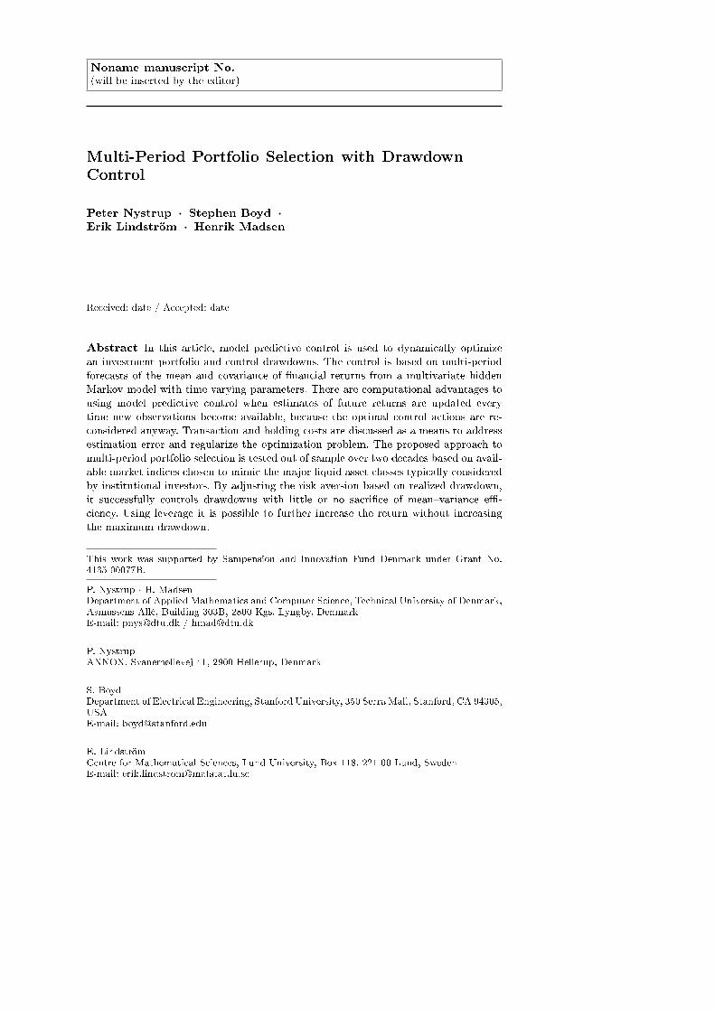
Figure 1: Development of the ten indices over the 20-year out-of-sample period.

This is only a subset of the indices considered in the out-of-sample test, as historicaldata is not available for EM high-yield bonds and in�ation-linked bonds. Furthermore,U.S. government bonds are a substitute for the Citi G7 government-bond index insample.

4.1.2 Out of sample

The asset universe considered in the out-of-sample test consists of DM and EM stocks,listed DM real estate, DM and EM high-yield bonds, gold, oil, corporate bonds, in�ation-linked bonds, and government bonds.8 All indices measure the total net return in USDwith a total of 5,185 daily closing prices per index covering the period from 1997through 2016.9 The �rst two years are used for initialization and the last 18 years areused for out-of-sample testing.

Figure 1 shows the ten indices' development over the 20-year out-of-sample period.There are large di�erences in the asset classes' behavior. The �nancial crisis in 2008stands out, in that respect, as the majority of the indices su�ered large losses in thisperiod.

Table 1 summarizes the indices' annualized excess return, excess risk, Sharpe ratio(SR)10, maximum drawdown11, and Calmar ratio (CR)12. The risk-free rate is assumed

8 The ten indices are MSCI World, MSCI Emerging Markets, FTSE EPRA/NAREIT De-veloped Real Estate, BofA Merrill Lynch U.S. High Yield, Barclays Emerging Markets HighYield, S&P GSCI Crude Oil (funded futures roll), LBMA Gold Price, Barclays U.S. Aggre-gate Corporate Bonds, Barclays World In�ation-Linked Bonds (hedged to USD), and Citi G7Government Bonds (hedged to USD).9 Days on which more than half of the indices had zero price change (19 days in total) have

been removed.10 The Sharpe ratio is the excess return divided by the excess risk (Sharpe, 1966, 1994).11 The maximum drawdown is the largest relative decline from a historical peak in the indexvalue, as de�ned in Sect. 2.4.12 The Calmar ratio is the annualized excess return divided by the maximum drawdown.


Table 1: Annualized performance of the ten indices over the 20-year out-of-sampleperiod in excess of the risk-free rate.

IndexExcess Excess Sharpe Maximum Calmarreturn risk ratio drawdown ratio

1. DM stocks 0.042 0.18 0.24 0.57 0.072. EM stocks 0.035 0.28 0.12 0.65 0.053. Real estate 0.054 0.22 0.24 0.72 0.074. DM high-yield bonds 0.050 0.12 0.42 0.35 0.145. EM high-yield bonds 0.077 0.13 0.61 0.36 0.216. Oil -0.046 0.42 -0.11 0.94 -0.057. Gold 0.038 0.16 0.23 0.45 0.098. Corporate bonds 0.040 0.06 0.68 0.16 0.259. In�ation-linked bonds 0.041 0.04 0.99 0.10 0.4010. Government bonds 0.032 0.03 1.17 0.05 0.65

to be the daily equivalent of the yield on a one-month U.S. treasury bill. The reportedexcess risks have been adjusted for autocorrelation using the procedure outlined byKinlaw et al (2014, 2015).13

The di�erences in performance are substantial. The oil price index is the only indexthat has had a negative excess return. The EM high-yield bond index realized thehighest excess return while in�ation-linked and government bonds realized the highestSharpe and Calmar ratios. Fixed income bene�ted from falling interest rates over theconsidered period.

4.2 In-sample training

In the in-sample training, the risk-aversion parameter is �xed at γ = 5 and portfolioperformance is evaluated in terms of SR, excess return, and annual turnover. Thechoice of γ = 5 results in portfolios with an excess risk similar to that of the equally-weighted 1/n portfolio (in Sect. 4.4 results are shown for a range of values of therisk-aversion parameter). Training is carried out solely for a long-only (LO) portfoliowith no leverage. Realized transaction costs, including bid�ask spread, are assumed tobe 10 basis points, and there is no transaction cost associated with the risk-free asset.The assets are assumed to be liquid enough compared to the total portfolio value thatprice impact can be ignored.14 Further, it is assumed that there are no holding costs.

Many of the hyperparameters are mutually dependent, which makes the in-sampletraining more challenging. For example, if the MPC planning horizon is doubled, trans-action costs also have to be doubled in order to maintain an approximately similarturnover.15 In addition, the optimal values of the MPC hyperparameters depend onthe choice of forecasting model.

13 The adjustment leads to the reported excess risks being higher than had they been annu-alized under the assumption of independence, as most of the indices display positive autocor-relation. The largest impact was on the excess risk of EM stocks that went from 0.20 to 0.28and the excess risk of DM high-yield bonds that went from 0.05 to 0.12.14 A transaction cost of 10 basis points is within the range of values estimated in empiricalstudies (see Pedersen, 2015, Chapter 5). It could be argued that transaction costs should belower for some indices and higher for others. This could easily be implemented as the elementsof κ1 and κ2 in (7) need not all be the same.15 See Grinold (2006); Boyd et al (2017) for more on amortization of transaction and holdingcosts.


To simplify the training task, it is divided into two steps. First, reasonable values ofthe MPC parameters are chosen and then used when testing di�erent forecasting mod-els. Second, the optimal MPC hyperparameters are found for the selected forecastingmodel. A �nal check is done to ensure that the model is still optimal for that choice ofMPC hyperparameters.

4.2.1 Forecasting model

Number of regimes and indices. At �rst, a multivariate HMM is �tted to all indicesat once. This results in a state sequence with low persistence and frequent switches,leading to excessive portfolio turnover and poor results. This is surprising given thelarge number of studies showing the value of DAA based on regime-switching models,in particular Nystrup et al (2017a) who used a univariate HMM of daily stock returnsto switch between prede�ned risk�on and risk�o� multi-asset portfolios. Inspired bythis approach, the states are instead estimated based on the two stock indices (DMand EM). The mean vector and covariance matrix in each state is still estimated basedon all indices, but the underlying state is estimated solely based on the two stockindices. This leads to a more persistent state sequence with fewer switches and betterportfolio performance. There is no bene�t to including additional indices in the stateestimation, as it increases the uncertainty. The stock indices appear to be su�cient inorder to capture important changes in risk and return. Models with two, three, andfour regimes are tested. There is no bene�t in going from two to three regimes and itis very hard to distinguish between four regimes out of sample.

E�ective memory length. E�ective memory lengths of T eff = 65, 130, 260, 520 daysare tested. The shorter the memory length used in the estimation, the higher the riskof having states with no visits and, consequently, probabilities converging to zero andnever recovering. This happens with memory lengths shorter than 100 days. The moreregimes, the longer the optimal memory length. With only two regimes, 130 days appearto be optimal.

Shrinkage factors. The shorter the memory length, the higher the optimal shrinkagefactor. Shrinkage factors of νi = 0.1, 0.2, . . . , 0.5 are tried in each of the two regimes.A shrinkage factor of 0.2 in the most frequent regime and 0.4 in the least visited regimeperforms best. The use of shrinkage signi�cantly improves the results, although theyare not overly sensitive to the speci�c choice of shrinkage factor within the tested range.

4.2.2 MPC parameters

Planning horizon. Planning horizons of H = 10, 15, . . . , 30 days are tested. 10 daysare found to be too few, while it appears that there is no bene�t in going beyond 15days.

Maximum holding constraint. Maximum holding constraintswmax = 0.2, 0.3, . . . , 0.5are tried. A maximum holding constraint ensures a minimum level of diversi�cation, butwith wmax = 0.2 there is limited possibility for deviating from the equally-weightedportfolio. As a compromise, a value of wmax = 0.4 is selected, but results are notsensitive to the particular choice within this range of values.


Transaction costs. Transaction costs (κ1)1:n = 0.0005, 0.001, . . . , 0.0055 are tested,while there is no transaction cost associated with the risk-free asset, i.e., (κ1)n+1 =

0. The term κT1 |wt − wt−1| is very e�ective at reducing portfolio turnover. Whenthis penalty is included, there is no additional bene�t from including a second termκT2 (wt − wt−1)

2. This squared term reduces the size of trades, but it appears thatit simply means that trades are split over multiple days and therefore delayed. Thisis not bene�cial given the assumption that there is no realized price-impact cost. Thevalue (κ1)1:n = 0.004 is selected.

Holding costs. Holding costs ρ2 = 0, 0.0005, . . . , 0.002 are tested. The holding costρT2 w

2t has a similar e�ect as the weight constraint (10): it encourages diversi�cation and

reduces the risk due to uncertainty in the covariance forecasts. Increasing ρ2 leads to amore diversi�ed and stable portfolio. If (ρ2)n+1 = 0, this will at the same time increasethe allocation to cash, which is undesirable. The value ρ2 = 0.0005 is selected. Thereis no bene�t to including an `1 term ρT1 |wt|, which leads to a more sparse portfolio.

4.3 Out-of-sample test results for γ0 = 5

Below, the performance of the MPC approach is evaluated for the above choice ofhyperparameters and compared to various benchmarks. First, results when γ0 = 5 arereported, and then in Sect. 4.4 results are analyzed for a range of values of γ0. In allcases it is assumed that assets can be bought and sold at the end of each trading day,subject to a 10 basis point transaction cost, and the fee for shorting assets is assumedto be equal to the risk-free rate. It is assumed that there are no price-impact or holdingcosts.

4.3.1 Allocations

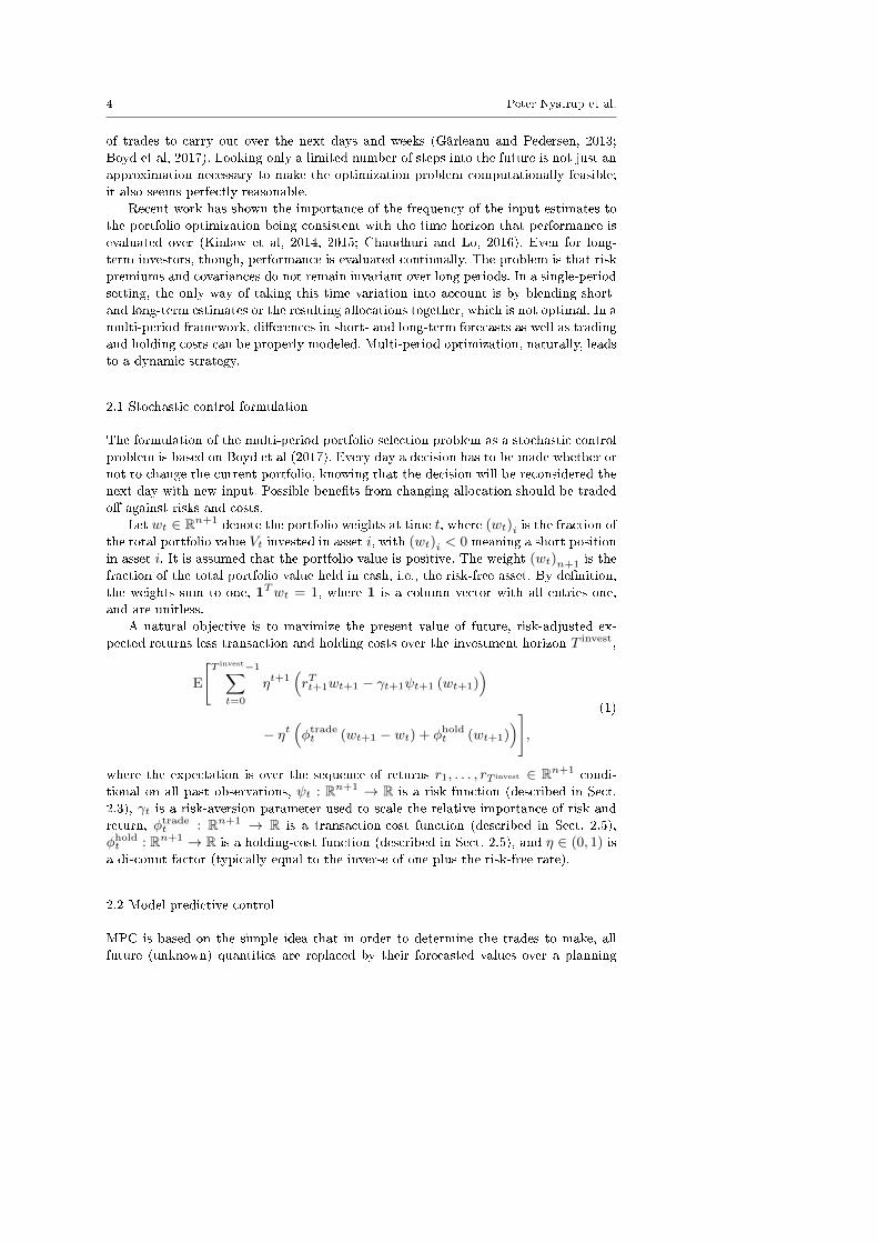
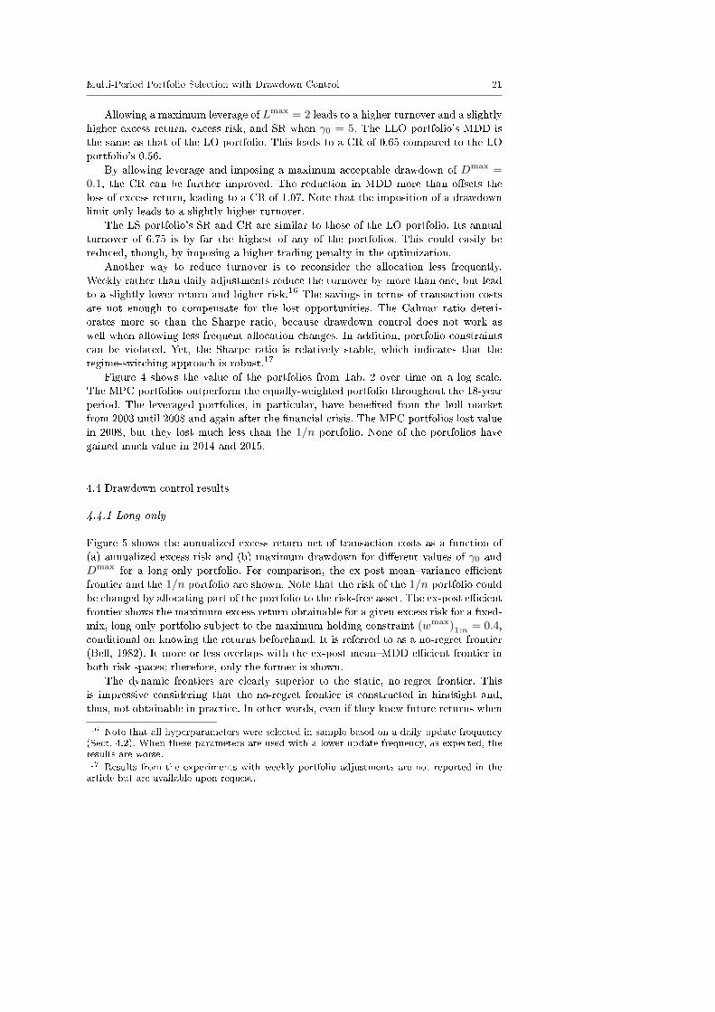
Figures 2 and 3 show the asset weights over time for a long-only and a long�short (LS)portfolio and for a leveraged long-only (LLO) portfolio without and with drawdowncontrol, respectively. The cost and weight parameters not mentioned in the �gure cap-tions are equal to zero. The portfolios always include multiple assets at a time due tothe imposed maximum holding (wmax)1:n = 0.4. The allocations change quite a bitover the test period, especially in the LS portfolio.

Leverage is primarily used between 2003 and mid-2006 and again from 2010 untilmid-2013. With the exception of these two periods, the four portfolios include holdingsin the risk-free asset most of the time in addition to some short positions in the LSportfolio. The impact of drawdown control on the allocation is most evident during the2008 crisis, where the LLO portfolio subject to drawdown control is fully allocated tocash.

4.3.2 Performance compared to �xed mix and 1/n

In Tab. 2, the MPC portfolios' annualized performance in excess of the risk-free ratewhen γ0 = 5 is compared to a �xed-mix (FM) portfolio and an equally-weighted (1/n)portfolio. The FM portfolio is rebalanced monthly to the average allocation of the LOportfolio over the entire 18-year test period. This means that the LO and the FM


Year

Assetweight

2000 2002 2004 2006 2008 2010 2012 2014 2016

0.0

0.2

0.4

0.6

0.8

1.0

TBill

IFL bonds

CORP bonds

GVT bonds

EM HY bonds

DM HY bonds

Oil

Gold

Real estate

EM stocks

DM stocks

(a) γ = 5, (κ1)1:n = 0.004, ρ2 = 0.0005, (wmax)1:n = 0.4, (wmax)n+1 = 1.

Year

Assetweight

2000 2002 2004 2006 2008 2010 2012 2014 2016

-1.0

-0.5

0.0

0.5

1.0

1.5

2.0

TBill

IFL bonds

CORP bonds

GVT bonds

EM HY bonds

DM HY bonds

Oil

Gold

Real estate

EM stocks

DM stocks

(b) γ = 5, (κ1)1:n = 0.004, ρ2 = 0.0005,(wmin

)1:n

= (wmax)1:n = 0.4,(wmin

)n+1

=

(wmax)n+1 = 1, Lmax = 2.

Figure 2: Asset weights over time for a long-only and a long�short portfolio.

Table 2: Annualized performance of MPC portfolios with γ0 = 5 compared to �xedmix and 1/n.

LO LLO LLODmax=0.1 LS FM 1/nExcess return 0.10 0.13 0.11 0.12 0.06 0.06Excess risk 0.11 0.12 0.11 0.12 0.12 0.11Sharpe ratio 0.97 1.01 1.00 1.01 0.51 0.52Maximum drawdown 0.19 0.19 0.10 0.23 0.38 0.37Calmar ratio 0.56 0.65 1.07 0.54 0.16 0.16Annual turnover 2.93 3.22 3.24 6.75 0.16 0.16

Notes: The �xed-mix portfolio is rebalanced monthly to the average allocation of the long-only

portfolio. The 1/n portfolio is rebalanced monthly. Transaction costs of 10 basis points per

transaction have been deducted. A borrowing fee equal to the risk-free rate has been deducted

for short positions.


Year

Assetweight

2000 2002 2004 2006 2008 2010 2012 2014 2016

-1.0

-0.5

0.0

0.5

1.0

1.5

2.0

TBill

IFL bonds

CORP bonds

GVT bonds

EM HY bonds

DM HY bonds

Oil

Gold

Real estate

EM stocks

DM stocks

(a) γ = 5, (κ1)1:n = 0.004, ρ2 = 0.0005, (wmax)1:n = 0.4,(wmin

)n+1

= (wmax)n+1 = 1.

Year

Assetweight

2000 2002 2004 2006 2008 2010 2012 2014 2016

-1.0

-0.5

0.0

0.5

1.0

1.5

2.0

TBill

IFL bonds

CORP bonds

GVT bonds

EM HY bonds

DM HY bonds

Oil

Gold

Real estate

EM stocks

DM stocks

(b) γ0 = 5, (κ1)1:n = 0.004, ρ2 = 0.0005, (wmax)1:n = 0.4,(wmin

)n+1

= (wmax)n+1 = 1,

Dmax = 0.1.

Figure 3: Asset weights over time for a leveraged long-only portfolio without and withdrawdown control.

portfolios have the same average allocation. Thus, di�erences in performance can onlybe attributed to timing and transaction costs. The 1/n portfolio is rebalanced monthlyto an equal allocation across all risky assets. The performance of FM and 1/n is fairlysimilar.

The LO portfolio's excess return is 445 basis points higher than that of the FMportfolio. This, combined with a slightly lower excess risk, leads to a SR of 0.97 com-pared to 0.51. DAA, even without drawdown control, leads to a MDD of 0.19 comparedto the FM portfolio's 0.38. This leads to a CR that is more than three times as high(0.56 compared to 0.16). The LO portfolio's annual turnover of 2.93 is a lot higherthan that of the FM portfolio, but the reported results are net of transaction costs of10 basis points per one-way transaction.


Allowing a maximum leverage of Lmax = 2 leads to a higher turnover and a slightlyhigher excess return, excess risk, and SR when γ0 = 5. The LLO portfolio's MDD isthe same as that of the LO portfolio. This leads to a CR of 0.65 compared to the LOportfolio's 0.56.

By allowing leverage and imposing a maximum acceptable drawdown of Dmax =0.1, the CR can be further improved. The reduction in MDD more than o�sets theloss of excess return, leading to a CR of 1.07. Note that the imposition of a drawdownlimit only leads to a slightly higher turnover.

The LS portfolio's SR and CR are similar to those of the LO portfolio. Its annualturnover of 6.75 is by far the highest of any of the portfolios. This could easily bereduced, though, by imposing a higher trading penalty in the optimization.

Another way to reduce turnover is to reconsider the allocation less frequently.Weekly rather than daily adjustments reduce the turnover by more than one, but leadto a slightly lower return and higher risk.16 The savings in terms of transaction costsare not enough to compensate for the lost opportunities. The Calmar ratio deteri-orates more so than the Sharpe ratio, because drawdown control does not work aswell when allowing less frequent allocation changes. In addition, portfolio constraintscan be violated. Yet, the Sharpe ratio is relatively stable, which indicates that theregime-switching approach is robust.17

Figure 4 shows the value of the portfolios from Tab. 2 over time on a log scale.The MPC portfolios outperform the equally-weighted portfolio throughout the 18-yearperiod. The leveraged portfolios, in particular, have bene�ted from the bull marketfrom 2003 until 2008 and again after the �nancial crisis. The MPC portfolios lost valuein 2008, but they lost much less than the 1/n portfolio. None of the portfolios havegained much value in 2014 and 2015.

4.4 Drawdown control results

4.4.1 Long only

Figure 5 shows the annualized excess return net of transaction costs as a function of(a) annualized excess risk and (b) maximum drawdown for di�erent values of γ0 andDmax for a long-only portfolio. For comparison, the ex-post mean�variance e�cientfrontier and the 1/n portfolio are shown. Note that the risk of the 1/n portfolio couldbe changed by allocating part of the portfolio to the risk-free asset. The ex-post e�cientfrontier shows the maximum excess return obtainable for a given excess risk for a �xed-mix, long-only portfolio subject to the maximum holding constraint (wmax)1:n = 0.4,conditional on knowing the returns beforehand. It is referred to as a no-regret frontier(Bell, 1982). It more or less overlaps with the ex-post mean�MDD e�cient frontier inboth risk spaces; therefore, only the former is shown.

The dynamic frontiers are clearly superior to the static, no-regret frontier. Thisis impressive considering that the no-regret frontier is constructed in hindsight and,thus, not obtainable in practice. In other words, even if they knew future returns when

16 Note that all hyperparameters were selected in sample based on a daily update frequency(Sect. 4.2). When these parameters are used with a lower update frequency, as expected, theresults are worse.17 Results from the experiments with weekly portfolio adjustments are not reported in thearticle but are available upon request.


100

200

500

1000

Year

Index

1999 2001 2003 2005 2007 2009 2011 2013 2015 2017

LLO

LS

LLODmax=0.1

LO

1/n

Figure 4: Performance over time of MPC portfolios with γ0 = 5 compared to anequally-weighted portfolio.Notes: Transaction costs of 10 basis points per transaction have been deducted. A borrowing

fee equal to the risk-free rate has been deducted for short positions.

choosing their benchmark, investors who insist on rebalancing to a static, diversi�edbenchmark could not have outperformed the dynamic strategies net of transactioncosts over the 18-year test period in terms of SR nor CR. The opportunity for DAAsigni�cantly expands the investment opportunity set; even so, this is a noteworthyresult.

The 1/n portfolio is ine�cient regardless of whether risk is measured by standarddeviation or MDD. This is no surprise given that it is based on a naive prior assumptionof equal returns, risks, and correlations across all assets. Yet, equally-weighted portfo-lios are often found to outperform mean�variance optimized portfolios out of sample(DeMiguel et al, 2009b; López de Prado, 2016). This suggests that the no-regret fron-tier would likely be closer to the 1/n portfolio than to the dynamic frontiers, had itnot bene�ted from hindsight.

Looking at the frontiers with and without drawdown control in Fig. 5a, it appearsthat drawdown control can be implemented with little loss of mean�variance e�ciency.By increasing the risk-aversion parameter as the drawdown approaches the maximumacceptable drawdown Dmax, a larger fraction of the portfolio is allocated to the risk-free asset, cf. Fig. 3b. Except for the transaction costs involved, this does not lead toa worse SR per se, but reduced risk-taking in periods with above-average SRs would.This is clearly not the case. Drawdown control simply leads to a higher average riskaversion.

From Fig. 5b it can be seen that the drawdown limit is breached�although not bymuch�when γ0 = 1. The success of the proposed approach to drawdown control is notvery sensitive to the choice of initial risk-aversion parameter γ0. Essentially, any valueγ0 ≥ 3 will work with a drawdown limit as tight as Dmax = 0.1. Drawdown controlis more sensitive to the allocation-update frequency, since optimal drawdown control


0.06 0.08 0.10 0.12 0.14

0.06

0.08

0.10

0.12

0.14

Annualized excess risk

Annualizedexcess

return

1/n

LO

LODmax=0.15

LODmax=0.1

No regret

(a)

0.10 0.15 0.20 0.25 0.30 0.35 0.40

0.06

0.08

0.10

0.12

0.14

Maximum drawdown

Annualizedexcess

return

1/n

LO

LODmax=0.15

LODmax=0.1

No regret

(b)

Figure 5: E�cient frontiers for di�erent values ofDmax compared to a no-regret frontierand an equally-weighted portfolio, when no leverage is allowed.Notes: The points, from right to left, correspond to γ0 = 1, 3, 5, 10, 15, 25. The 1/n portfolio is

rebalanced monthly. Transaction costs of 10 basis points per transaction have been deducted.

requires continuous trading. Yet, daily allocation updates are su�cient for it to workfor reasonable values of γ0 and Dmax.

4.4.2 Long�short

Figure 6 shows the annualized excess return net of transaction costs as a function of (a)annualized excess risk and (b) maximum drawdown for di�erent values of γ0 and Dmax


0.06 0.08 0.10 0.12 0.14

0.06

0.08

0.10

0.12

0.14

Annualized excess risk

Annualizedexcess

return

1/n

LS

LLO

LLODmax=0.15

LLODmax=0.1

No regret

(a)

0.10 0.15 0.20 0.25 0.30 0.35 0.40

0.06

0.08

0.10

0.12

0.14

Maximum drawdown

Annualizedexcess

return

1/n

LS

LLO

LLODmax=0.15

LLODmax=0.1

No regret

(b)

Figure 6: E�cient frontiers for di�erent values ofDmax compared to a no-regret frontierand an equally-weighted portfolio, when leverage and short positions are allowed.Notes: The points, from right to left, correspond to γ0 = 1, 3, 5, 10, 15, 25. The 1/n portfolio is

rebalanced monthly. Transaction costs of 10 basis points per transaction have been deducted.

The maximum leverage allowed is Lmax = 2.

for LS and LLO portfolios. For comparison, the ex-post mean�variance e�cient frontierand the 1/n portfolio are shown. The ex-post e�cient frontier gives the maximumexcess return obtainable for a given excess risk for a �xed-mix, long�short portfoliosubject to the same holding and leverage constraints,

(wmin

)1:n

= (wmax)1:n = 0.4and Lmax = 2, conditional on knowing the returns beforehand.


In Fig. 6a, the possibility of using leverage or taking short positions extends thee�cient frontier. Leverage can be applied to increase risk while maintaining diversi�-cation, rather than concentrating the portfolio in a few assets. This reduces the gapbetween the dynamic frontiers and the no-regret frontier.

In Fig. 6b, the di�erence between the dynamic frontiers and the no-regret frontieris still substantial. Again, the ex-post mean�variance e�cient frontier more or lessoverlaps with the ex-post mean�MDD e�cient frontier; therefore, only the former isshown. By taking a dynamic approach, the maximum drawdown can be reduced by0.25, while maintaining the same excess return.

The combination of leverage and drawdown control is powerful. Compared to Fig.5b, it is possible to increase the excess return by several hundred basis points withoutsu�ering a larger MDD by combining the use of leverage with drawdown control. Thepossible excess return is bounded by the drawdown limit. Seeking excess return beyondthis boundary by removing the drawdown limit and lowering γ0 comes at the cost of asigni�cantly increased MDD. This is true regardless of whether leverage can be applied.

5 Conclusion

By adjusting the risk aversion based on realized drawdown, the proposed approach tomulti-period portfolio selection based on MPC successfully controlled drawdowns withlittle or no sacri�ce of mean�variance e�ciency. The empirical testing showed thatperformance could be signi�cantly improved by reducing realized risk and MDD usingthis dynamic approach. In fact, even if they knew future returns when choosing theirbenchmark, investors who insisted on rebalancing to a static benchmark allocationcould not have outperformed the dynamic approach net of transaction costs over the18-year out-of-sample test period. The combination of leverage and drawdown controlwas particularly successful, as it was possible to increase the excess return by severalhundred basis points without su�ering a larger MDD.

The MPC approach to multi-period portfolio selection has potential in practical ap-plications, because it is computationally fast. This makes it feasible to consider a largeuniverse of assets and implement important constraints and costs. When combined withan adaptive forecasting method it provides a �exible framework for incorporating newinformation into a portfolio as it becomes available. This should de�nitely be useful infuture research, when evaluating the performance of return-prediction models.

Acknowledgements The authors are thankful for the helpful comments from the responsibleeditor Stavros A. Zenios and two anonymous referees.

References

Almgren R, Chriss N (2001) Optimal execution of portfolio transactions. Journal ofRisk 3(2):5�39

Ang A, Bekaert G (2004) How regimes a�ect asset allocation. Financial Analysts Jour-nal 60(2):86�99

Ang A, Timmermann A (2012) Regime changes and �nancial markets. Annual Reviewof Financial Economics 4(1):313�337


Ardia D, Bolliger G, Boudt K, Gagnon-Fleury JP (2017) The impact of covariancemisspeci�cation in risk-based portfolios. Annals of Operations Research 254(1-2):1�16

Artzner P, Delbaen F, Eber JM, Heath D (1999) Coherent measures of risk. Mathe-matical Finance 9(3):203�228

Bae GI, Kim WC, Mulvey JM (2014) Dynamic asset allocation for varied �nancial mar-kets under regime switching framework. European Journal of Operational Research234(2):450�458

Bell DE (1982) Regret in decision making under uncertainty. Operations Research30(5):961�981

Bellman R (1956) Dynamic programming and Lagrange multipliers. Proceedings of theNational Academy of Sciences 42(10):767�769

Bemporad A, Bellucci L, Gabbriellini T (2014) Dynamic option hedging via stochas-tic model predictive control based on scenario simulation. Quantitative Finance14(10):1739�1751

Bertsimas D, Lauprete GJ, Samarov A (2004) Shortfall as a risk measure: properties,optimization and applications. Journal of Economic Dynamics & Control 28(7):1353�1381

Black F, Jones RW (1987) Simplifying portfolio insurance. Journal of Portfolio Man-agement 14(1):48�51

Black F, Litterman R (1992) Global portfolio optimization. Financial Analysts Journal48(5):28�43

Black F, Perold AF (1992) Theory of constant proportion portfolio insurance. Journalof Economic Dynamics & Control 16(3�4):403�426

Black F, Scholes M (1973) The pricing of options and corporate liabilities. Journal ofPolitical Economy 81(3):637�654

Boyd S, Vandenberghe L (2004) Convex Optimization. Cambridge University Press,New York

Boyd S, Mueller MT, O'Donoghue B, Wang Y (2014) Performance bounds and subop-timal policies for multi-period investment. Foundations and Trends in Optimization1(1):1�72

Boyd S, Busseti E, Diamond S, Kahn RN, Koh K, Nystrup P, Speth J (2017) Multi-period trading via convex optimization. Foundations and Trends in Optimization3(1):1�76

Broadie M (1993) Computing e�cient frontiers using estimated parameters. Annals ofOperations Research 45(1):21�58

Brodie J, Daubechies I, Mol CD, Giannone D, Loris I (2009) Sparse and stableMarkowitz portfolios. Proceedings of the National Academy of Sciences of the UnitedStates of America 106(30):12267�12272

Bulla J, Mergner S, Bulla I, Sesboüé A, Chesneau C (2011) Markov-switching assetallocation: Do pro�table strategies exist? Journal of Asset Management 12(5):310�321

Chaudhuri SE, Lo AW (2016) Spectral portfolio theory. Available at SSRN 2788999 pp1�44

Chopra VK, Ziemba WT (1993) The e�ect of errors in means, variances, and covari-ances on optimal portfolio choice. Journal of Portfolio Management 19(2):6�11

Cui X, Gao J, Li X, Li D (2014) Optimal multi-period mean�variance policy underno-shorting constraint. European Journal of Operational Research 234(2):459�468


Dai M, Xu ZQ, Zhou XY (2010) Continuous-time Markowitz's model with transactioncosts. SIAM Journal on Financial Mathematics 1(1):96�125

Dantzig GB, Infanger G (1993) Multi-stage stochastic linear programs for portfoliooptimization. Annals of Operations Research 45(1):59�76

DeMiguel V, Garlappi L, Nogales F, Uppal R (2009a) A generalized approach to port-folio optimization: Improving performance by constraining portfolio norms. Manage-ment Science 55(5):798�812

DeMiguel V, Garlappi L, Uppal R (2009b) Optimal versus naive diversi�cation: Howine�cient is the 1/N portfolio strategy? Review of Financial Studies 22(5):1915�1953

Diamond S, Boyd S (2016) CVXPY: A Python-embedded modeling language for convexoptimization. Journal of Machine Learning Research 17(83):1�5

Dias JG, Vermunt JK, Ramos S (2015) Clustering �nancial time series: New insightsfrom an extended hidden Markov model. European Journal of Operational Research243(3):852�864

Dohi T, Osaki S (1993) A note on portfolio optimization with path-dependent utility.Annals of Operations Research 45(1):77�90

Domahidi A, Chu E, Boyd S (2013) ECOS: An SOCP solver for embedded systems.In: Proceedings of the 12th European Control Conference, pp 3071�3076

Downing C, Madhavan A, Ulitsky A, Singh A (2015) Portfolio construction and tailrisk. Journal of Portfolio Management 42(1):85�102

Fabozzi FJ, Huang D, Zhou G (2010) Robust portfolios: contributions from operationsresearch and �nance. Annals of Operations Research 176(1):191�220

Fastrich B, Paterlini S, Winker P (2015) Constructing optimal sparse portfolios usingregularization methods. Computational Management Science 12(3):417�434

Fiecas M, Franke J, von Sachs R, Kamgaing JT (2017) Shrinkage estimation for mul-tivariate hidden Markov models. Journal of the American Statistical Association112(517):424�435

Fleming J, Kirby C, Ostdiek B (2001) The economic value of volatility timing. Journalof Finance 56(1):329�352

Frühwirth-Schnatter S (2006) Finite Mixture and Markov Switching Models. Springer,New York

Garlappi L, Uppal R, Wang T (2006) Portfolio selection with parameter and modeluncertainty: A multi-prior approach. Review of Financial Studies 20(1):41�81

Gârleanu N, Pedersen LH (2013) Dynamic trading with predictable returns and trans-action costs. Journal of Finance 68(6):2309�2340

Goltz F, Martellini L, Simsek KD (2008) Optimal static allocation decisions in thepresence of portfolio insurance. Journal of Investment Management 6(2):37�56

Grinold RC (2006) A dynamic model of portfolio management. Journal of InvestmentManagement 4(2):5�22

Grinold RC, Kahn RN (2000) Active Portfolio Management: A Quantitative Approachfor Providing Superior Returns and Controlling Risk, 2nd edn. McGraw�Hill, NewYork

Grossman SJ, Zhou Z (1993) Optimal investment strategies for controlling drawdowns.Mathematical Finance 3(3):241�276

Guidolin M, Timmermann A (2007) Asset allocation under multivariate regime switch-ing. Journal of Economic Dynamics and Control 31(11):3503�3544

Gülp�nar N, Rustem B (2007) Worst-case robust decisions for multi-period mean�variance portfolio optimization. European Journal of Operational Research183(3):981�1000


Herzog F, Dondi G, Geering HP (2007) Stochastic model predictive control andportfolio optimization. International Journal of Theoretical and Applied Finance10(2):203�233

Ho M, Sun Z, Xin J (2015) Weighted elastic net penalized mean�variance portfoliodesign and computation. SIAM Journal on Financial Mathematics 6(1):1220�1244

Ibragimov R, Ja�ee D, Walden J (2011) Diversi�cation disasters. Journal of FinancialEconomics 99(2):333�348

Ilmanen A (2012) Do �nancial markets reward buying or selling insurance and lotterytickets? Financial Analysts Journal 68(5):26�36

Jagannathan R, Ma T (2003) Risk reduction in large portfolios: Why imposing thewrong constraints helps. Journal of Finance 58(4):1651�1683

Jorion P (1985) International portfolio diversi�cation with estimation risk. Journal ofBusiness 58(3):259�278

Kan R, Zhou G (2007) Optimal portfolio choice with parameter uncertainty. Journalof Financial and Quantitative Analysis 42(3):621�656

Khreich W, Granger E, Miri A, Sabourin R (2012) A survey of techniques for incre-mental learning of HMM parameters. Information Sciences 197:105�130

Kinlaw W, Kritzman M, Turkington D (2014) The divergence of high- and low-frequency estimation: Causes and consequences. Journal of Portfolio Management40(5):156�168

Kinlaw W, Kritzman M, Turkington D (2015) The divergence of high- and low-frequency estimation: Implications for performance measurement. Journal of Port-folio Management 41(3):14�21

Kolm P, Tütüncü R, Fabozzi F (2014) 60 years of portfolio optimization: Practical chal-lenges and current trends. European Journal of Operational Research 234(2):356�371

Kritzman M, Li Y (2010) Skulls, �nancial turbulence, and risk management. FinancialAnalysts Journal 66(5):30�41

Kritzman M, Page S, Turkington D (2012) Regime shifts: Implications for dynamicstrategies. Financial Analysts Journal 68(3):22�39

Ledoit O, Wolf M (2003) Improved estimation of the covariance matrix of stock returnswith an application to portfolio selection. Journal of Empirical Finance 10(5):603�621

Ledoit O, Wolf M (2004) A well-conditioned estimator for large-dimensional covariancematrices. Journal of Multivariate Analysis 88(2):365�411

Leland HE (1980) Who should buy portfolio insurance? Journal of Finance 35(2):581�594

Li J (2015) Sparse and stable portfolio selection with parameter uncertainty. Journalof Business & Economic Statistics 33(3):381�392

Lim AE, Shanthikumar JG, Vahn GY (2011) Conditional value-at-risk in portfoliooptimization: Coherent but fragile. Operations Research Letters 39(3):163�171

Mandelbrot B (1963) The variation of certain speculative prices. Journal of Business36(4):394�419

Markowitz H (1952) Portfolio selection. Journal of Finance 7(1):77�91Markowitz H (2014) Mean�variance approximations to expected utility. European Jour-nal of Operational Research 234(2):346�355

Mattingley J, Boyd S (2012) CVXGEN: a code generator for embedded convex opti-mization. Optimization and Engineering 13(1):1�27

Mei X, DeMiguel V, Nogales FJ (2016) Multiperiod portfolio optimization with multi-ple risky assets and general transaction costs. Journal of Banking & Finance 69:108�


120Meindl PJ, Primbs JA (2008) Dynamic hedging of single and multi-dimensional optionswith transaction costs: a generalized utility maximization approach. QuantitativeFinance 8(3):299�312

Merton RC (1969) Lifetime portfolio selection under uncertainty: The continuous-timecase. Review of Economics and Statistics 51(3):247�257

Merton RC (1973) Theory of rational option pricing. Bell Journal of Economics andManagement Science 4(1):141�183

Merton RC (1980) On estimating the expected return on the market: An exploratoryinvestigation. Journal of Financial Economics 8(4):323�361

Michaud RO (1989) The Markowitz optimization Enigma: Is 'optimized' optimal? Fi-nancial Analysts Journal 45(1):31�42

Moreira A, Muir T (2017) Volatility-managed portfolios. Journal of Finance72(4):1611�1644

Mossin J (1968) Optimal multiperiod portfolio policies. Journal of Business 41(2):215�229

Mulvey JM, Shetty B (2004) Financial planning via multi-stage stochastic optimiza-tion. Computers & Operations Research 31(1):1�20

von Neumann J, Morgenstern O (1953) Theory of Games and Economic Behavior, 3rdedn. Princeton University Press, Princeton

Nystrup P, Hansen BW, Madsen H, Lindström E (2015a) Regime-based versus staticasset allocation: Letting the data speak. Journal of Portfolio Management 42(1):103�109

Nystrup P, Madsen H, Lindström E (2015b) Stylised facts of �nancial time series andhidden Markov models in continuous time. Quantitative Finance 15(9):1531�1541

Nystrup P, Hansen BW, Larsen HO, Madsen H, Lindström E (2017a) Dynamic al-location or diversi�cation: A regime-based approach to multiple assets. Journal ofPortfolio Management 44(2):62�73

Nystrup P, Madsen H, Lindström E (2017b) Long memory of �nancial time seriesand hidden Markov models with time-varying parameters. Journal of Forecasting36(8):989�1002

Nystrup P, Madsen H, Lindström E (2018) Dynamic portfolio optimization acrosshidden market regimes. Quantitative Finance 18(1):83�95

Pedersen LH (2009) When everyone runs for the exit. International Journal of CentralBanking 5(4):177�199

Pedersen LH (2015) E�ciently ine�cient: how smart money invests and market pricesare determined. Princeton University Press, Princeton

P�nar MÇ (2007) Robust scenario optimization based on downside-risk measure formulti-period portfolio selection. OR Spectrum 29(2):295�309

López de Prado M (2016) Building diversi�ed portfolios that outperform out of sample.Journal of Portfolio Management 42(4):59�69

Rockafellar RT, Uryasev S (2000) Optimization of conditional value-at-risk. Journal ofRisk 2(3):21�42

Rubinstein M, Leland HE (1981) Replicating options with positions in stock and cash.Financial Analysts Journal 37(4):63�72

Rydén T, Teräsvirta T, Åsbrink S (1998) Stylized facts of daily return series and thehidden Markov model. Journal of Applied Econometrics 13(3):217�244

Samuelson PA (1969) Lifetime portfolio selection by dynamic stochastic programming.Review of Economics and Statistics 51(3):239�246


Scutellà MG, Recchia R (2013) Robust portfolio asset allocation and risk measures.Annals of Operations Research 204(1):145�169

Sharpe WF (1966) Mutual fund performance. Journal of Business 39(1):119�138Sharpe WF (1994) The Sharpe ratio. Journal of Portfolio Management 21(1):49�58Smidl V, Gustafsson F (2012) Bayesian estimation of forgetting factor in adaptive�ltering and change detection. In: Proceedings of the 2012 IEEE Statistical SignalProcessing Workshop, pp 197�200

Stein C (1956) Inadmissibility of the usual estimator for the mean of a multivariatenormal distribution. In: Proceedings of the Third Berkeley Symposium on Mathe-matical Statistics and Probability, University of California Press, Berkeley, vol 1, pp197�206

Stenger B, Ramesh V, Paragios N, Coetzee F, Buhmann JM (2001) Topology freehidden Markov models: Application to background modeling. In: Proceedings of theEighth IEEE International Conference on Computer Vision, vol 1, pp 294�301

Stoyanov SV, Rachev ST, Fabozzi FJ (2012) Sensitivity of portfolio VaR and CVaR toportfolio return characteristics. Annals of Operations Research 205(1):169�187

Zenios SA (2007) Practical Financial Optimization: Decision Making for FinancialEngineers. Blackwell, Malden

Zhou G, Zhu Y (2010) Is the recent �nancial crisis really a "once-in-a-century" event?Financial Analysts Journal 66(1):24�27

Documents

Multi-period portfolio selection with drawdown control · multi-period framework, di erences in short- and long-term forecasts as well as trading and holding costs can be properly