Embed Size (px)
Citation preview
Multi-period Mean-Variance Portfolio Optimization basedon Monte-Carlo Simulation
F. Cong ∗1 and C.W. Oosterlee1,2
1TU Delft, Delft Institute of Applied Mathematics, Delft, The Netherlands2CWI-Centrum Wiskunde & Informatica, Amsterdam, The Netherlands
November 26, 2015
Abstract
We propose a simulation-based approach for solving the constrained dynamic mean-variance portfolio management problem. For this dynamic optimization problem, we firstconsider a sub-optimal strategy, called the multi-stage strategy, which can be utilizedin a forward fashion. Then, based on this fast yet sub-optimal strategy, we proposea backward recursive programming approach to improve it. We design the backwardrecursion algorithm such that the result is guaranteed to converge to a solution, whichis at least as good as the one generated by the multi-stage strategy. In our numericaltests, highly satisfactory asset allocations are obtained for dynamic portfolio managementproblems with realistic constraints on the control variables.
Keywords: Dynamic portfolio management · Mean-variance optimization · Constrainedoptimization · Simulation method · Least-square regression
1 Introduction
Since Markowitz’s pioneering work [Mar52] on a single-period investment model, themean-variance portfolio optimization problem has become a cornerstone of investmentmanagement in both academic and industrial fields. An interesting topic, extendingMarkowitz’s work, is to consider the mean-variance target for a continuous or multi-periodoptimization problem. Along with introducing dynamic control into the optimizationprocess, constraints on the controls can be included.
In some situations, the constrained dynamic mean-variance optimization problem canbe solved analytically. For example, [LZL02] solves this portfolio management problemwith no-shorting of stock allowed and [BJPZ05] solves the problem with bankruptcyprohibition. In [FLLL10], the authors investigate the mean-variance problem with aborrowing constraint, where the investor faces a borrowing rate different from the risk-free saving rate. However, all this research is performed in the framework of continuousoptimization. In fact, as mentioned in [CGLL14], the continuous constrained optimizationproblem is usually easier than the discrete one. In general, an elegant analytic mean-variance formulation can be derived in case of a complete market, where re-balancing can
∗Corresponding author. Email: [email protected]
1
be performed continuously and there are no constraints on the controls and no jumps inasset dynamics. If we consider a realistic problem which is designed in an incompletemarket, it will be difficult to obtain analytic solutions and thus utilizing computationaltechniques to calculate numerical solutions is our preferred choice.
The nonlinearity of conditional variance is the main obstacle for solving the dynamicmean-variance optimization problem. In [ZL00] and [LN00], an embedding technique, bywhich the mean-variance problem is transformed into a stochastic linear-quadratic (LQ)problem, is introduced. For the linear-quadratic problem, an investor does not need tochoose a trade-off parameter between mean and variance. Instead, she decides a finaloptimization target of her investment. In [ZL00] and [LN00], it is proved that varying thefinal investment target traces out the same efficient frontier as varying the mean-variancetrade-off parameters. To generate the efficient frontier of the mean-variance optimizationproblem, we can thus solve the LQ problem with different target parameters.
To solve the constrained target-based problem, the Hamilton-Jacobi-Bellman partialdifferential equation (HJB PDE) is often considered. Accurate results can be generatedby solving the HJB PDEs for a one-dimensional scenario. For example, [WF10] solvesthe continuous constrained mean-variance optimization problem with various constraintsand the risky asset following geometric Brownian motion. The authors of [DF14b] solve asimilar problem with the risky asset following jump-diffusion dynamics. In both papers,realistic constraints are cast on the control variables. However, it is rather expensive toimplement the algorithm, which is based on solving the HJB PDE, for a problem withseveral risky assets. Reducing the dimensionality of such a problem is a potential solution.However, when constraints are introduced, the assumption for establishing the well-knownmutual fund theory is not valid and the ratio between the different risky assets is notconstant any more. A general multi-dimensional problem can hardly be transformed intoa one-dimensional problem.
To deal with the curse of dimensionality, using Monte-Carlo simulation constitutes apossible solution. A well-known simulation-based dynamic portfolio management algo-rithm is proposed in [BGSCS05]. However, they discuss a problem where the investor hasconstant relative risk aversion. For such problems, the investor’s optimal asset allocationis only influenced by the dynamics of the risky asset, so dynamic programming can beperformed after the (forward) simulation of the risky assets. For an investor with othertypes of risk aversion, her optimal intermediate decisions usually do not only depend onthe dynamics of the risky asset but also on the amount of wealth at that time. The simu-lation approach proposed in [BGSCS05] is therefore not feasible for a general investmentproblem. Solving the constrained dynamic mean-variance problem based on Monte-Carlosimulation is the focus of our work.
Our methods depend on transforming the mean-variance problem into the LQ prob-lem, which is a target-based problem. In [BC10], the investment strategy for solving theLQ problem is named the pre-commitment strategy, which however does not guaranteetime consistency. As mentioned in [WF11], a time-consistent strategy can be formulatedas a pre-commitment strategy plus time consistent constraints on the asset allocations.Thus, the pre-commitment strategy generally yields an efficient frontier which is superiorto the one generated by a time consistent strategy. In this paper, we will contributeto pre-commitment strategies and propose two solutions for the dynamic mean-varianceproblem, one is performed in a forward manner and the other in a backward manner.
In the forward approach, we decompose the dynamic optimization problem into sev-eral static optimization problems by specifying intermediate investment targets at allre-balancing time steps. A reasonable approximation for the optimal controls can bedetermined at each single stage and solving the problems at all stages provides us asub-optimal strategy called the “multi-stage strategy”. We prove that the multi-stage
2

strategy is the optimal strategy when there are no constraints on the asset allocations.Although the multi-stage strategy becomes sub-optimal in case of constrained controls,it is straight-forward to implement the multi-stage strategy for either high dimensionalproblems or problems with complicated constraints. While experimenting, we observethat the multi-stage strategy can yield highly satisfactory results compared to the refer-ence solutions.
The main challenge to perform backward programming for a constrained optimiza-tion problem is that the value function at each time step is non-smooth and thus theoptimality cannot be computed efficiently by solving the corresponding first order con-ditions. To tackle this problem, we utilize the idea of differential dynamic programming[JM70], by which a stochastic control problem is solved by a local optimization strategy,and we come up with a backward recursive approach. Our backward recursive program-ming algorithm is an iterative method. With special design of the algorithm, we canguarantee that the outcome converges to a solution, which is not worse than the solutiongenerated by the multi-stage strategy. In the backward process, conditional expectationsare calculated recursively via cross-path least-squares regression. To make this numericalapproach stable, we implement the “bundling” and “regress-later” techniques, proposedin [JO15]. The idea of “bundling” is highly compatible with the local optimization in dif-ferential dynamic programming. The backward recursive programming is initiated witha reasonable guess for the asset allocations, which can be, but is not restricted to, theone generated by the multi-stage strategy. In our tests with the initial allocation gener-ated by the multi-stage strategy, we achieve highly satisfactory results after at most fourbackward iterations. Like the multi-stage strategy, the backward recursive programmingcan be performed highly efficiently. In our numerical tests, one iteration of the backwardrecursive programming only takes a few seconds.
This paper is organized as follows. In Section 2, we introduce the formulation ofthe dynamic mean-variance problem and the embedding into a stochastic LQ problem.Section 3 describes the multi-stage strategy. The optimality of the multi-stage strategyin the unconstrained case is proved in Section 3.1. In Section 4, the backward dynamicprogramming method is presented. Section 5 displays several realistic constraints for theportfolio management problems and in Section 6 numerical tests are performed for bothone- and two-dimensional problems. We conclude in Section 7.
2 Problem Formulation
This section describes the dynamic portfolio optimization problem for a defined contribu-tion pension plan. We assume that the financial market is defined on a probability space(Ω,F , Ft0≤t≤T ,P) with finite time horizon [0, T ]. The state space Ω is the set of allrealizations of the financial market within the time horizon [0, T ]. F is the sigma algebraof events at time T , i.e. F = FT . We assume that the filtration Ft0≤t≤T is generatedby the price processes of the financial market and augmented with the null sets of F .Probability measure P is defined on F .
For convenience, we consider a portfolio consisting of two assets, one risk-free and onerisky. To extend the analysis to a problem with more than one risky asset is feasible. Weconsider a portfolio, which can be traded at discrete opportunities1, t ∈ [0,∆t, . . . , T−∆t],before terminal time T . At each trading time t, an investor decides her trading strategyto maximize the expectation of the terminal wealth and to minimize the investment risk.
1We assume that the re-balancing times are equidistantly spread and the total number of re-balancingopportunities before terminal time T is M . The time step ∆t between two re-balancing days is T
M .
3
Formally, the investor’s problem is given by
vt(Wt) = maxxsT−∆t
s=t
E[WT |Wt]− λ ·Var[WT |Wt]
, (1)
subject to the wealth restriction:
Ws+∆t = Ws · (xsRes +Rf ) + C ·∆t, s = t, t+ ∆, . . . , T −∆t.
Here xs denotes the asset allocation of the investor’s wealth in the risky asset in the period[s, s+ ∆t). It is assumed that the admissible investment strategy xt is an Ft-measurableMarkov control, i.e. xt ∈ Ft. Rf is the return of the risk-free asset in one time step,which is assumed to be constant for simplicity, and Res is the excess return of the riskyasset during [s, s + ∆t). We assume that the excess returns RetT−∆t
t=0 are statisticallyindependent2. C · ∆t stands for a contribution of the investor in the portfolio during[s, s+ ∆t), and a negative C can be interpreted as a constant withdrawal of the investorfrom the portfolio. The risk aversion attitude of the investor is denoted by λ, which is atrade-off factor between maximizing the profit and minimizing the risk. vt(Wt) is termedthe value function, which measures the investor’s investment opportunities at time t withwealth Wt.
Remark 2.1. When the mean-variance optimization problem proposed by Equation (1)is convex, then solving Equation (1) is equivalent to determination of the Pareto optimalpoints, i.e. solving
minxsT−∆t
s=t
Var[WT |Wt]
s.t. E[WT |Wt] ≥ d,
with a suitable choice of d. However, when the problem is not convex, solving Equation(1) generates Pareto optimal points, but not all of them.
The difficulty of solving this mean-variance optimization problem is caused by thenonlinearity of conditional variances, namely Var[Var[WT |Ft]|Fs] 6= Var[WT |Fs], s ≤ t,which makes the well-known dynamic programming valuation approach not applicable.To tackle this problem, the original mean-variance equations can be transformed intoanother framework as done in [ZL00, LN00, WF10]. The following theorem supports thetransformation.
Theorem 2.2. If x∗sT−∆ts=t is the optimal control for the problem defined in Equation
(1), then x∗sT−∆ts=t is also the optimal control for the following problem:
minxsT−∆t
s=t
E[(WT −
γ
2)2|Wt]
(2)
where γ = 1λ + 2Ex∗ [WT |Wt]. Here the operator Ex∗ [·] denotes the expectation of the
investor’s terminal wealth if she invests according to the optimal strategy x∗sT−∆ts=t .
Proof. See [LN00].
2For a risky asset with dynamics following geometric Brownian motion or a Levy process, the independencestructure is valid. For some problems where the asset returns are directly defined, for example, as model-freedata, the independence assumption is also correct. For a VAR or GARCH model, this assumption is, however,not satisfied.
4
Based on this theorem, the original mean-variance problem can be embedded intoa tractable auxiliary LQ problem. The investment strategy corresponding to this LQproblem is called the pre-commitment strategy. This technique can also be interpreted astransforming the original mean-variance problem into a target-based optimization prob-lem, which has been discussed in [HV02, GHV04]. For numerical computation, the pre-commitment optimization problem as shown in Equation (2) is usually formulated as anHJB PDE and realistic constraints on either controls or state variables can be corre-spondingly established as boundary conditions. In this manner, [WF10] solves the mean-variance problem numerically and derives a solution to the constrained pre-commitmentstrategy.
However, even for the LQ problem, casting constraints in the numerical approach isin general not trivial. Imposing constraints on the controls will substantially change theformulation of the problem and make it nontrivial to solve the problem efficiently. Thereasoning is as follows. For the unconstrained problem, the value function at each timestep forms a smooth function and thus the optimality can be obtained by solving thefirst-order conditions associated to this smooth function. Adding constraints will removethe smoothness of the value function. Derivative-based optimization techniques cannotbe applied in this situation and the optimality has to be computed by grid-searching onthe whole domain of possible controls, for example, as in [WF10].
In the following section, we propose a sub-optimal yet highly efficient strategy for themean-variance portfolio management problem. In this strategy, we avoid dealing withnon-smooth value functions even if there are constraints on the controls. It is possibleto extend this sub-optimal strategy to high-dimensional problems and to problems withcomplicated asset dynamics.
3 A Forward Solution: the Multi-stage Strategy
When we prescribe constraints on the allocations, neither the original mean-variancestrategy associated to solving Equation (1) nor the pre-commitment strategy associatedto solving Equation (2) is easy to obtain.
Here we treat the mean-variance optimization problem from a different angle. Afterwriting it into the pre-commitment form, or equivalently into the target-based form, theobjective of the reformulated optimization problem is to minimize the difference betweenthe final wealth and a predetermined target. Hence the optimization problem at time treads:
J∗pct (Wt) := minxsT−∆t
s=t
E[(WT −
γ
2)2|Wt]
, (3)
or, in a recursive fashion,
J∗pct (Wt) = minxt
E[J∗pct+∆t(Wt+∆t)|Wt]
, (4)
with J∗pcT (WT ) = (WT − γ2 )2.
At the state (t,Wt), i.e. time t and wealth Wt, the value function Jt(Wt) dependson all optimal allocations at subsequent time steps. That is why generally this kind ofoptimization problem has to be solved in a backward recursive fashion via, for exam-ple, solving the HJB PDEs or backward stochastic differential equations (BSDEs) withconditions at the terminal time.
Solving this dynamic programming problem numerically in a backward recursive fash-ion suffers from two problems. First, solving the optimality, especially for constrainedcases, at each time step may be difficult or computationally expensive. Secondly, since
5
we use the value function to transmit information between two recursive steps, the erroraccumulates as the recursion proceeds.
Reflection on these two issues leads us to define a sub-optimal strategy, which doesnot involve these two types of errors, which we call the multi-stage strategy.
Notice that at the terminal time, our target is γ2 . Then, at state (t,Wt), in the
multi-stage strategy we choose xt to be:
x∗mst := arg minxt
E[(Wt · (xtRet +Rf ) + C ·∆t− δt+∆t
)2∣∣∣Wt
], (5)
where
δt =
γ2 − C ·∆t ·
1−(Rf )(T−t)/∆t
1−Rf(Rf )(T−t)/∆t . (6)
So, here we do not consider the optimality in the future, but perform a single-stage, orstatic, optimization with respect to a given target value.
Equation (6) is straightforward. We set an intermediate target at time t such that oncewe achieve this target, we can put all the money in the risk-free asset and at the terminaltime the wealth reaches the final target. Therefore, this intermediate target is computedby discounting the final target while taking into account the constant contribution.
Considering an intermediate wealth target is not a new idea. In [GHV06], the authorsstudy the target-based optimization problem for a defined-contribution pension plan andmake use of intermediate targets mainly for calculating the cumulative losses throughoutthe management period. In [CLWZ12], the authors consider an intermediate thresh-old. Once the portfolio wealth exceeded this threshold, they proved that withdrawing asuitable amount of money from the portfolio will not influence the performance of theportfolio in the sense of mean-variance optimization.
Since our multi-stage method merely depends on solving a single-stage optimizationproblem at each time point, the problem can be solved in a forward fashion:
• First, we generate the intermediate target values at each time step.
• Then, starting at the initial state we compute the optimal allocation step by stepuntil the terminal time.
If we consider no periodic contributions, i.e. C = 0, we can rewrite the optimalallocation for the pre-commitment problem in Equation (3) as:
x∗pct (Wt) = arg minxt
E[(Wt · (xtRet +Rf ) ·
T−∆t∏s=t+∆t
(x∗pcs Res +Rf )− γ
2
)2∣∣∣Wt
], (7)
where x∗pcs T−∆ts=t+∆t denote the optimal allocations at times s = t+ ∆t, . . . , T −∆t.
In this scenario the multi-stage optimization problem can be formulated as:
x∗mst (Wt) = arg minxt
E[(Wt · (xtRet +Rf ) ·
T−∆t∏s=t+∆t
(Rf )− γ
2
)2∣∣∣Wt
]. (8)
We see that the objective of the multi-stage optimization is indeed different from thatof the original optimization. Instead of considering the true optimization x∗pcs T−∆t
s=t+∆t,
we “specify” x∗mss T−∆ts=t+∆t to be zero. That is why we call the multi-stage solution sub-
optimal. However, by sacrificing the possibility to pursue the optimality, we also gainsome profits which are discussed in the next section.
Remark 3.1. The multi-stage strategy can be treated as a “greedy strategy” for thestochastic optimization problem [BMOW13]. In each stage, we minimize the distancebetween our wealth and the target of the current stage.
6
Remark 3.2. One crucial restriction for constructing the multi-stage strategy is that thereshould be a risk-free asset in the market. Regarding the wealth-to-income case discussedin [WF10], we cannot find a risk-free part in the market and therefore cannot derive theintermediate optimization target for our multi-stage approach.
Gains and Losses
By the multi-stage strategy, we avoid the backward recursive programming by construct-ing determined intermediate targets. Since there is no error accumulation in the recursion,the optimization problem solved at the intermediate time step is unbiased3 to what wedesigned it to be.
On the other hand, casting constraints on this sub-optimal strategy is trivial. Since atevery time step we deal with a quadratic optimization problem in the multi-stage strategy,solving the constrained optimization problem can usually be performed efficiently. Inthe one-dimensional case, for example, solving the constrained quadratic optimizationproblem is equivalent to first solving the unconstrained problem to generate the optimalcontrol and then truncating this optimal control by the constraints.
The drawback of the multi-stage strategy is also obvious: instead of tackling theoriginal optimization problem, we work on a tailored one. The optimal control for thesub-optimal problem may differ from that for the original problem, so the mean-variancepair corresponding to this sub-optimal strategy may be located below the optimal efficientfrontier. However, in the next section we will prove that in some situations the optimalallocation for the multi-stage strategy is exactly the same as that for the original pre-commitment strategy.
3.1 Equivalence In the Unconstrained Case
In this section, we restrict ourselves to the situation where there is no periodic contribu-tion, i.e. C = 0. Extending the analysis to the case where C 6= 0 is however possible.Under the following condition, we can prove that the multi-stage strategy and the pre-commitment strategy are equivalent for generating the optimal asset allocations.
Condition 3.3. The asset allocations at each time step are unconstrained.
In this case, we can obtain the analytic form of the value function at intermediatetime steps for the pre-commitment problem.
Lemma 3.4. For the pre-commitment problem shown in Equation (3), the value functionJt(Wt) can be formulated as:
Jt(Wt) = Lt ·(Wt · (Rf )(T−t)/∆t − γ
2
)2, (9)
where Lt =∏Ts=t ls with lt defined as follows:
lt = 1− E[Ret ]2
E[(Ret )2], t = 0,∆t, . . . , T −∆t,
lT = 1.
Proof. At time step T , the value function is known as:
JT (WT ) = (WT −γ
2)2,
3In the traditional backward programming approach, since numerical errors cumulate alongside the recursiveprocedure, biases in the intermediate optimization problems exist.
7
which satisfies Equation (9). At time step T −∆t, the value function reads:
JT−∆t(WT−∆t)
= maxxT−∆t
E[JT (WT−∆t · (xT−∆tR
eT−∆t +Rf ))|WT−∆t]
= maxxT−∆t
E[(WT−∆t · (xT−∆tR
eT−∆t +Rf )− γ
2
)2∣∣∣WT−∆t
]. (10)
To obtain the analytic form of JT−∆t(WT−∆t), we first need to determine the optimalasset allocation x∗T−∆t, which satisfies:
x∗T−∆t = arg minxT−∆t
E[(WT−∆t · (xT−∆tR
eT−∆t +Rf )− γ
2
)2∣∣∣WT−∆t
].
Solving the first-order conditions of the optimality problem gives us that x∗T−∆t is thesolution to the following equation:
E[(WT−∆t · (xT−∆tR
eT−∆t +Rf )− γ
2
)·WT−∆tR
eT−∆t
∣∣∣WT−∆t
]= 0.
So, the optimal allocation x∗T−∆t can be calculated as:
x∗T−∆t =(γ2 −WT−∆tRf ) · E[ReT−∆t]
WT−∆t · E[(ReT−∆t)2]
. (11)
Inserting Equation (11) into Equation (10) yields:
JT−∆t(WT−∆t)
=E[(
1−E[ReT−∆t] ·ReT−∆t
E[(ReT−∆t)2]
)2]·(WT−∆tRf −
γ
2
)2
=(
1−E[ReT−∆t]
2
E[(ReT−∆t)2]
)·(WT−∆tRf −
γ
2
)2.
It is clear that the value function at time step T −∆t has the same form as in Equation(9). For the remaining time steps, we can formulate the value functions by backwardinduction.
Assume that at time step t+ ∆t we have:
Jt+∆t(Wt+∆t) = Lt+∆t ·(Wt+∆t · (Rf )(T−t)/∆t−1 − γ
2
)2.
Then at time step t, the value function can be formulated as:
Jt(Wt)
= maxxt
E[Jt+∆t(Wt · (xtRet +Rf ))|Wt]
= max
xt
E[Lt+∆t ·
(Wt · (xtRet +Rf ) · (Rf )(T−t)/∆t−1 − γ
2
)2∣∣∣Wt
]=E[Lt+∆t] ·max
xt
E[(Wt · (xtRet +Rf ) · (Rf )(T−t)/∆t−1 − γ
2
)2∣∣∣Wt
].
Here the last equality is based on the independence of the excess returns. Solving thefirst-order condition yields:
x∗t =(γ2 −Wt · (Rf )(T−t)/∆t) · E[Ret ]
Wt · (Rf )(T−t)/∆t−1 · E[(Ret )2]. (12)
8

and the corresponding value function reads:
Jt(Wt)
=Lt+∆t ·(
1− E[Ret ]2
E[(Ret )2]
)·(Wt · (Rf )(T−t)/∆t − γ
2
)2
=Lt ·(Wt · (Rf )(T−t)/∆t − γ
2
)2.
Thus we finalize the proof.
Remark 3.5. The optimal asset allocation shown in Equation (12) is exactly the sameas the one proposed in [LN00] for the one-dimensional case.
With Lemma 3.4, we can prove the equivalence between our multi-stage strategyand the pre-commitment strategy. Formally, the equivalence is shown in the followingtheorem.
Theorem 3.6. For a mean-variance portfolio management problem, where Condition 3.3is satisfied, the optimal control for the multi-stage strategy and for the pre-commitmentstrategy are identical. That is, x∗pct and x∗mst , as respectively shown in Equations (7) and(8), are equal at each time step t.
Proof. For the pre-commitment problem, the optimal control x∗pct reads:
x∗pct = arg minxt
E[Jt+∆t(Wt · (xtRet +Rf ))|Wt]
.
Using the form of the value function Jt+∆t(·) as shown in Lemma 3.4, we find:
x∗pct = arg minxt
E[Lt+∆t ·
(Wt · (xtRet +Rf ) · (Rf )(T−t)/∆t−1 − γ
2
)2∣∣∣Wt
].
Because of the independence of the excess returns, we can treat Lt+∆t as a constant factorand thus the minimization problem turns out to be:
x∗pct = arg minxt
E[(Wt · (xtRet +Rf ) · (Rf )(T−t)/∆t−1 − γ
2
)2∣∣∣Wt
], (13)
Since the right-hand-sides of Equations (8) and (13) have the same form, the proof isfinished.
Notice that we only establish the equivalence between the multi-stage problem and thepre-commitment problem when the excess returns are independent and the allocationsare unconstrained. If we equip the excess returns with path-dependent dynamics or castconstraints on the allocations, the equivalence may be lost. However, based on numericalresults in [WF12], we know that the efficient frontiers for different investment strategiesmay differ significantly in the unconstrained case but the differences are relatively smallerwhen constraints are introduced. In our numerical approach we only apply the multi-stage strategy to generate asset allocations and then the mean-variance pair is calculatedby combining the simulated trajectories and the corresponding “sub-optimal” allocations.As spotted in [WF10], small errors in asset allocations may not influence the accuracy ofthe mean-variance pair dramatically.
Even though the multi-stage strategy may be not equivalent to the pre-commitmentstrategy in some situations, it can serve as a sub-optimal solution to the constraineddynamic mean-variance portfolio optimization problem. If some other accurate solutionsexist, the corresponding efficient frontiers should be at least above that of the multi-stage
9
strategy. Moreover, for some numerical methods that depend on iteratively updating theasset allocations, a reasonable initial guess can be provided by the multi-stage method,see Section 4.
The authors of [SB08] proposed a similar technique to the multi-stage strategy forthe quadratic convex optimization problem. Our research differs in two aspects. First,instead of dealing with one optimization problem which can yield one point on the ef-ficient frontier, we consider a series of optimization problems which generate results toconstruct the whole efficient frontier. We find that the multi-stage strategy is particularlysatisfactory when the investor is highly risk averse. However, in case the investor is lessrisk averse, the sub-optimal strategy turns out to be problematic. For this, we propose abackward dynamic programming approach, which is different from the forward strategy.
Remark 3.7. As discussed in [CLWZ12, DF14a], a semi-self-financing strategy existswhich is better than the pre-commitment strategy. In that strategy, a positive amount ofmoney is withdrawn from the portfolio when the wealth in the portfolio is above a deter-mined value. Similarly, the multi-stage strategy can be adjusted in this respect. However,since the improvement achieved by breaking the self-financing is not significant, we willnot deal with the semi-self-financing multi-stage strategy in this paper.
4 Backward Recursive Programming
In the preceding sections, we considered the “greedy policy” for the dynamic optimizationproblem, and therefore the constrained dynamic mean-variance problem can be solved in aforward fashion via Monte-Carlo simulation. Except for the unconstrained case, the multi-stage strategy allocation is generally not the optimal solution to the dynamic optimizationproblem. In order to get the optimal solution, we have to consider a backward dynamicprogramming solution. In this section, we present an approach to perform backwardrecursive calculation based on the solution of the multi-stage strategy.
Benefit from the Constraints
In general, constraints complicate dynamic optimization problems. For an unconstrainedoptimization problem, the value functions are smooth, so the optimality can be obtainedby solving the first-order conditions. When constraints are introduced, the smoothnessof the value functions is destroyed and derivative-based optimization is thus no longerfeasible. However, if we treat the constraints differently, they can also be “helpful”.
Consider an optimization problem at the state (t,Wt):
Jt(Wt) = minxt∈A
E[Jt+∆t(Wt+∆t)|Wt]
, (14)
where A is the admissible set for the asset allocation xt. Jt(·) is the value function attime t. When A 6= R, this is a constrained problem, which may not be easy to solve.However, if we consider a special case where A = xt|xt = K, i.e. xt is restricted to bea constant, the constrained problem becomes trivial. In fact, since we know that xt hasto be constant, the “optimal” solution in the admissible set is known immediately.
Using the multi-stage strategy, we obtain x∗mst , which may be a reasonable approx-imation of x∗t , which denotes the real optimal allocation. If we construct a truncatedadmissible control set, Aη = [x∗mst − η, x∗mst + η], the solution to the following optimiza-tion problem
Jt(Wt) = minxt∈Aη
E[Jt+∆t(Wt+∆t)|Wt]
,
10
should be the same as that of the problem shown in Equation (14). Assuming that theoptimal allocations for the state (t,Wt) are in an interval [x∗mst −η, x∗mst +η], the investor’soptimal wealth Wt+∆t should be located in the domain4:
Dt+∆t := Wt+∆t|Wt+∆t = Wt · (xt ·Ret +Rf ) + C ·∆t, xt ∈ Aη.
We further transform the original optimization problem shown in Equation (14) to be:
Jt(Wt) = minxt∈A
E[Jt+∆t(Wt+∆t)|Wt,Wt+∆t ∈ Dt+∆t]
, (15)
where an additional condition is introduced into the conditional expectation. Insteadof considering the optimization problem on the whole domain of Wt+∆t, we restrict theoptimization problem to a finite domain Dt+∆t and thus establish a local optimizationproblem. For solving the stochastic optimization problem at state (t,Wt), we focus onthe value function Jt+∆t(Wt+∆t) on a finite interval Dt+∆t.
Benefit from bundling
By means of the constraints, the original problem in Equation (14) is simplified to atruncated problem in Equation (15). To solve this truncated problem, we first need todetermine the value function Jt+∆t(Wt+∆t) on domain Dt+∆t. A common simulation-based approach is that we vary xt around x∗mst and perform sub-simulation, which ishowever involved and costly. One way to avoid sub-simulation is by plain Monte-Carlosimulation combined with bundling. Using the bundling technique, the domain Dt+∆t
can be approximated by:
Dt+∆t = Wt+∆t|Wt+∆t = Wt · (x∗mst ·Ret +Rf ) + C ·∆t, Wt ∈ Bδ,
where Bδ = [Wt − δ,Wt + δ]. So, instead of varying xt, we vary Wt by considering thepaths whose states are around (t,Wt). For more details about bundling, we refer thereaders to [JO15].
4.1 Backward Programming Algorithm
Now we formally describe the algorithm for the backward programming stage.
• Step 1: Initiation:Generate an initial guess of optimal asset allocations xtT−∆t
t=0 and simulate thepaths of optimal wealth values Wt(i)Ni=1, t = 0, . . . , T . At the terminal time T , wehave the determined value function JT (WT ).The following three steps are subsequently performed, recursively, backward in time,at t = T −∆t, . . . ,∆t, 0.
• Step 2: SolvingBundle paths into B partitions, where each bundle contains a similar number ofpaths and the paths inside a bundle have similar values at time t. Denote thewealth values associated to the paths in the bundle by W b
t (i)NBi=1, where NB isthe number of paths in the bundle. Within each bundle, we perform the followingprocedure.
4This domain is much smaller than the domain obtained without restricting xt. To avoid unnecessarytechnicalities, we assume that the wealth process is locally bounded.
11
– For paths in the bundle, we have the corresponding wealth values W bt+∆t(i)
NBi=1
and the continuation values Jbt+∆t(i)NBi=1 at time t+∆t. So, a function f bt+∆t(·),
which satisfies Jbt+∆t = f bt+∆t(Wbt+∆t) on the local domain, can be determined
by regression5.
– For all paths in the bundle, since the value function f bt+∆t(Wbt+∆t) has been
approximated, we solve the optimization problem by calculating the first-orderconditions. In this way, we get new asset allocations xbt(i)
NBi=1.
– Since the wealth values W bt (i)NBi=1 and the allocations xbt(i)
NBi=1 are known,
by regression we can also compute the new continuation values Jbt (i)NBi=1. Here
Jbt (i) is the expectation of Jt+∆t(Wt+∆t) conditional on W bt (i) and xbt(i), that
is,Jbt (i) = E[Jt+∆t(Wt+∆t)|Wt = W b
t (i), xt = xbt(i)].
• Step 3: UpdatingFor the paths in a bundle, since we have an old guess xbt
NBi=1 for the asset allocations,
by regression we can also calculate the old continuation values Jbt (i)NBi=1. For the
i-th path, if Jbt (i) > Jbt (i), we choose xbt(i) as the updated allocation. Otherwise weretain the initial allocation. We denote the updated allocations by xbt(i)
NBi=1.
• Step 4: EvolvingOnce the updated allocations xbt(i)
NBi=1 are obtained, again by regression we can
calculate the “updated” continuation values Jbt (i)NBi=1 and proceed with the back-
ward recursion.
In the algorithm, at each time step and inside each bundle, four regression steps areperformed. Especially, the last three regression steps are added for calculating valuefunctions. Since the value function is used to evolve information between time steps, anerror in calculating them will accumulate due to recursion. In general, we can settle thisproblem by using a very large number of simulations, which is however expensive. In ournumerical approach we always use the “regress-later” technique as applied in [CO15].
When we use the regression, polynomials up to order two are considered as basisfunctions. For the unconstrained problem, the value function is a quadratic function, sothis choice of basis functions is sufficient. In the constrained case, although the valuefunction is non-smooth, it is still piecewise quadratic as stated in [FLLL10]. Since theregression is performed with respect to paths in the same bundle, it is a local regression,i.e. local polynomial fitting. In all, our algorithm, which adopts second order localpolynomial fitting to approximate piecewise quadratic functions, should yield satisfactoryresults.
After one iteration of the algorithm, we will obtain an “updated” asset allocation ateach time step. The algorithm can be performed iteratively. In the remaining part of thissection, we will prove that these iterations will lead to a convergent result.
Remark 4.1. In the engineering field, this type of dynamic programming is called dif-ferential dynamic programming. For more details, we refer the reader to [JM70] and[TES08].
5Here regression refers to the technique of approximating the target function by a truncated basis functionexpansion, where the expansion coefficients are determined by minimizing the approximation error in the leastsquares sense.
12

4.2 Convergence of the Backward Recursive Programming
For the dynamic backward recursive programming, we have
Jt(Wt) = minxt
E[Jt+∆t(Wt · (xtRet +Rf ) + C ·∆t)|Wt]
, t = T −∆t, . . . , 0,
where the expectation is taken over the return Ret . This recursion can be written as:
Jt = ΨtJt+∆t, t = T −∆t, . . . , 0,
where Ψt is the Bellman operator, defined as
(Ψth)(Wt) = minxt
E[h(Wt · (xtRet +Rf ) + C · t)|Wt]
. (16)
According to [Ber95], the Bellman operator has the monotonicity property, which isdescribed by the following lemma.
Lemma 4.2 (Monotonicity). For any f : R → R and g : R → R,
f ≤ g ⇒ Ψtf ≤ Ψtg,
where the inequalities are interpreted pointwise, and Ψt is as in (16).
We can prove the following proposition:
Proposition 4.3. The backward recursive updating process, as explained in Section 4.1,converges. That is: there exists a function J∗0 (·) satisfying
J∗0 (W0) = limk→+∞
J(k)0 (W0),
where J(k)0 (W0) denotes the value function at initial state after k iterations of the algo-
rithm in Section 4.1.
Proof. The proof is directly based on the design of the backward recursive programmingalgorithm and the Monotonicity Lemma 4.2. Since at each iteration, we compare theprevious and the new allocations and retain the one which generates a smaller valuefunction and since the Bellman operator preserves monotonicity, we get:
J(1)0 (W0) ≥ J (2)
0 (W0) ≥ · · · ≥ J (k)0 (W0), k = 1, . . . , kmax.
Since the value function is positive, according to the Monotone Convergence Theorem,we can finalize the proof.
Whereas the convergence can be proved, the convergence rate is not determined. Theconvergence rate depends on the smoothness of the value functions and the initial guessof the allocations. For example, for a smooth quadratic value function, any initial guessshould give the correct result after one iteration. On the other hand, if we choose zeroas the initial guess for all the asset allocations, the solution can never depart from thestationary point, which is generated by the risk-free investment strategy. In our numericaltests, we always achieve satisfactory results using the initial guess of the asset allocationsgenerated by the multi-stage strategy.
On the other hand, the solution of our backward recursive approach is not guar-anteed to be the optimal one. We call this algorithm “sub-optimal” because a bias isintroduced when we approximate the non-smooth value function by piecewise quadraticpolynomials. Although the numerical tests indicate that our algorithm generates highlysatisfactory solutions, we expect that in case the value function is highly non-smooth theapproximation bias in our algorithm will be large and the accuracy of our algorithm maybe unsatisfactory.
13
5 Constraints on the Asset Allocations
From the perspective of real-life applications, introducing constraints on the asset allo-cations is important. For example, when an investor goes bankrupt, she should not beallowed to manage her portfolio any more. Besides, according to regulations for banks,the leverage ratio should be bounded. In this section, we will formulate controls on theasset allocations.
5.1 No Bankruptcy constraint
In this paper, the “no bankruptcy” constraint implies that there is zero probability ofbankruptcy when the constraint is cast on the asset allocations. To ensure that theallocation at time t does not lead to bankruptcy at time t+ ∆t, we need:
Wt · (xtRet +Rf ) + C∆t ≥ 0. (17)
Note that if there is a “no bankruptcy” constraint, definitely we have Wt > 0. Therefore,to guarantee that Equation (17) is valid, we need:
xtRet ≥ −Rf −
C∆t
Wt. (18)
Since Ret = exp(ret )−Rf , where re is a a random variable, we require
−Rf ≥ −Rfxt− C∆t
Wt · xtand xt ≥ 0.
to ensure Equation (18) to be valid. Reformulating these equations, we have:
0 ≤ xt ≤ 1 +C∆t
Wt ·Rf. (19)
The “no bankruptcy” constraint given by Equation (19) implies limWt→0(xt ·Wt) = 0, asgiven in [WF10, WF11] for the continuous portfolio optimization problem. Our version ofthe “no bankruptcy” constraint for the multi-period case is stronger than the constraintin [WF10, WF11]. Rather than specifying that wealth should not be invested in therisky asset when the total wealth amount is close to zero, our constraint also indicatesthat special consideration to the asset allocation should be given even though the wealthamount is far above zero. This is due to the difference between continuous and discretere-balancing. In the latter case, since we cannot manage the portfolio between two re-balancing opportunities, it is possible that the investor goes bankrupt after an extrememarket movement. To avoid this situation, we need to impose more strict constraintson the asset allocations, which is however not necessary for a continuous re-balancingproblem.
5.2 No Bankruptcy constraint with 1− 2α% Certainty
When the wealth in a portfolio is large, according to the discussion in the last subsection,the upper bound for “no bankruptcy” constraint (19) will be close to 1, which is quiterigorous. Using this as the upper bound protects an investor from bankruptcy only in therare case that the risky asset yields zero return. A possible way to relieve this constraintis to take the possibility of bankruptcy into account.
Assume that the α- and the (1−α)- quantiles of the excess return Ret are respectivelyRe,αt and Re,1−αt . Then with certainty 1− 2α% and the constraints shown below, we can
14
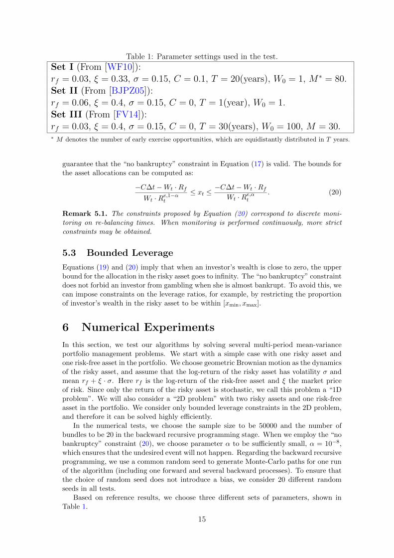
Table 1: Parameter settings used in the test.
Set I (From [WF10]):rf = 0.03, ξ = 0.33, σ = 0.15, C = 0.1, T = 20(years), W0 = 1, M ∗ = 80.Set II (From [BJPZ05]):rf = 0.06, ξ = 0.4, σ = 0.15, C = 0, T = 1(year), W0 = 1.Set III (From [FV14]):rf = 0.03, ξ = 0.4, σ = 0.15, C = 0, T = 30(years), W0 = 100, M = 30.∗ M denotes the number of early exercise opportunities, which are equidistantly distributed in T years.
guarantee that the “no bankruptcy” constraint in Equation (17) is valid. The bounds forthe asset allocations can be computed as:
−C∆t−Wt ·RfWt ·Re,1−αt
≤ xt ≤−C∆t−Wt ·Rf
Wt ·Re,αt. (20)
Remark 5.1. The constraints proposed by Equation (20) correspond to discrete moni-toring on re-balancing times. When monitoring is performed continuously, more strictconstraints may be obtained.
5.3 Bounded Leverage
Equations (19) and (20) imply that when an investor’s wealth is close to zero, the upperbound for the allocation in the risky asset goes to infinity. The “no bankruptcy” constraintdoes not forbid an investor from gambling when she is almost bankrupt. To avoid this, wecan impose constraints on the leverage ratios, for example, by restricting the proportionof investor’s wealth in the risky asset to be within [xmin, xmax].
6 Numerical Experiments
In this section, we test our algorithms by solving several multi-period mean-varianceportfolio management problems. We start with a simple case with one risky asset andone risk-free asset in the portfolio. We choose geometric Brownian motion as the dynamicsof the risky asset, and assume that the log-return of the risky asset has volatility σ andmean rf + ξ · σ. Here rf is the log-return of the risk-free asset and ξ the market priceof risk. Since only the return of the risky asset is stochastic, we call this problem a “1Dproblem”. We will also consider a “2D problem” with two risky assets and one risk-freeasset in the portfolio. We consider only bounded leverage constraints in the 2D problem,and therefore it can be solved highly efficiently.
In the numerical tests, we choose the sample size to be 50000 and the number ofbundles to be 20 in the backward recursive programming stage. When we employ the “nobankruptcy” constraint (20), we choose parameter α to be sufficiently small, α = 10−8,which ensures that the undesired event will not happen. Regarding the backward recursiveprogramming, we use a common random seed to generate Monte-Carlo paths for one runof the algorithm (including one forward and several backward processes). To ensure thatthe choice of random seed does not introduce a bias, we consider 20 different randomseeds in all tests.
Based on reference results, we choose three different sets of parameters, shown inTable 1.
15
0 1 2 3 4 5 6 7 8 9 10
5
10
15
20
25
30
std0[W
*
T]
E0[W
* T]
allow bankruptcy
no bankruptcy
bounded control
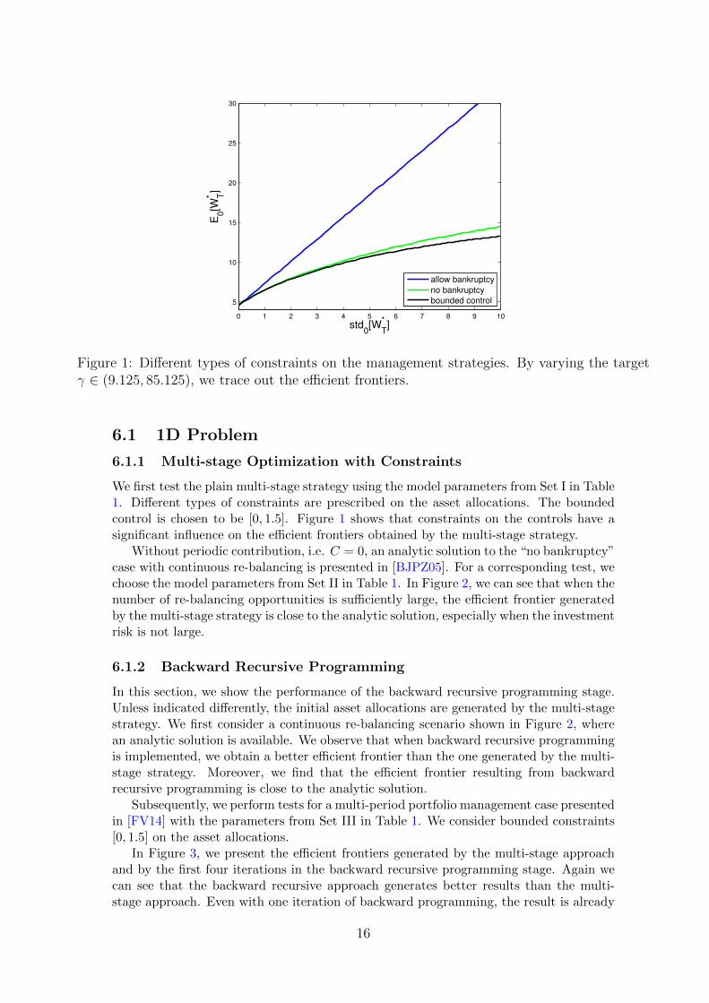
Figure 1: Different types of constraints on the management strategies. By varying the targetγ ∈ (9.125, 85.125), we trace out the efficient frontiers.
6.1 1D Problem
6.1.1 Multi-stage Optimization with Constraints
We first test the plain multi-stage strategy using the model parameters from Set I in Table1. Different types of constraints are prescribed on the asset allocations. The boundedcontrol is chosen to be [0, 1.5]. Figure 1 shows that constraints on the controls have asignificant influence on the efficient frontiers obtained by the multi-stage strategy.
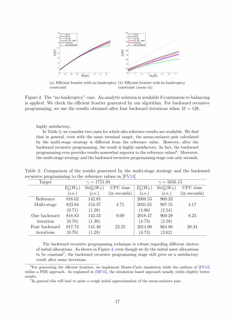
Without periodic contribution, i.e. C = 0, an analytic solution to the “no bankruptcy”case with continuous re-balancing is presented in [BJPZ05]. For a corresponding test, wechoose the model parameters from Set II in Table 1. In Figure 2, we can see that when thenumber of re-balancing opportunities is sufficiently large, the efficient frontier generatedby the multi-stage strategy is close to the analytic solution, especially when the investmentrisk is not large.
6.1.2 Backward Recursive Programming
In this section, we show the performance of the backward recursive programming stage.Unless indicated differently, the initial asset allocations are generated by the multi-stagestrategy. We first consider a continuous re-balancing scenario shown in Figure 2, wherean analytic solution is available. We observe that when backward recursive programmingis implemented, we obtain a better efficient frontier than the one generated by the multi-stage strategy. Moreover, we find that the efficient frontier resulting from backwardrecursive programming is close to the analytic solution.
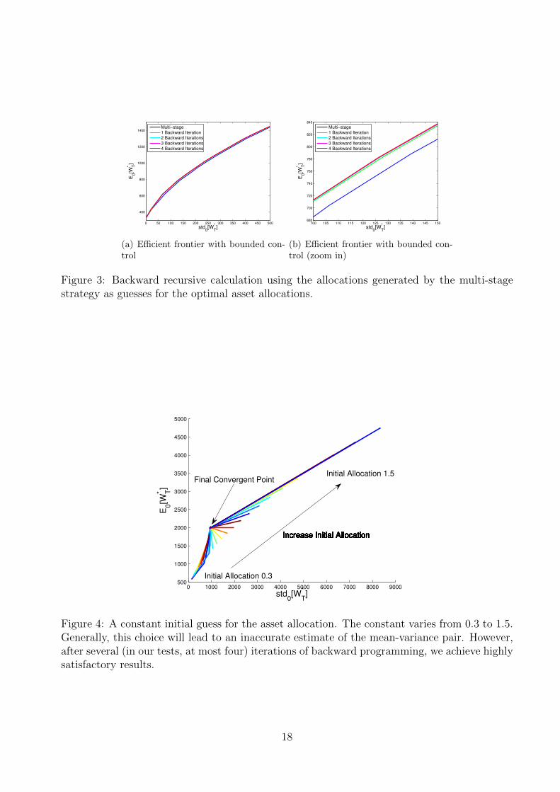
Subsequently, we perform tests for a multi-period portfolio management case presentedin [FV14] with the parameters from Set III in Table 1. We consider bounded constraints[0, 1.5] on the asset allocations.
In Figure 3, we present the efficient frontiers generated by the multi-stage approachand by the first four iterations in the backward recursive programming stage. Again wecan see that the backward recursive approach generates better results than the multi-stage approach. Even with one iteration of backward programming, the result is already
16
0 0.2 0.4 0.6 0.8 1 1.2 1.4 1.61
1.1
1.2
1.3
1.4
1.5
1.6
1.7
1.8
std0[W
*
T]
E0[W
* T]
M=32
M=64
M=128
M=128 + BRP
Analytical
No Constraints
(a) Efficient frontier with no bankruptcyconstraint
1 1.1 1.2 1.3 1.4 1.5 1.6 1.71.4
1.45
1.5
1.55
1.6
1.65
1.7
1.75
1.8
1.85
std0[W
*
T]
E0[W
* T]
M=32
M=64
M=128
M=128 + BRP
Analytical
No Constraints
(b) Efficient frontier with no bankruptcyconstraint (zoom in)
Figure 2: The “no bankruptcy” case. An analytic solution is available if continuous re-balancingis applied. We check the efficient frontier generated by our algorithm. For backward recursiveprogramming, we use the results obtained after four backward iterations when M = 128.
highly satisfactory.In Table 2, we consider two cases for which also reference results are available. We find
that in general, even with the same terminal target, the mean-variance pair calculatedby the multi-stage strategy is different from the reference value. However, after thebackward recursive programming, the result is highly satisfactory. In fact, the backwardprogramming even provides results somewhat superior to the reference values6. Moreover,the multi-stage strategy and the backward recursive programming stage cost only seconds.
Table 2: Comparison of the results generated by the multi-stage strategy and the backwardrecursive programming to the reference values in [FV14].
Target γ = 1751.94 γ = 5856.15E∗0(WT ) Std∗0(WT ) CPU time E∗0(WT ) Std∗0(WT ) CPU time
(s.e.) (s.e.) (in seconds) (s.e.) (s.e.) (in seconds)Reference 816.62 142.85 2008.55 969.33
Multi-stage 823.84 154.37 4.71 2031.65 987.55 4.17(0.71) (1.28) (4.86) (2.54)
One backward 818.83 143.33 9.09 2018.47 969.29 8.23iteration (0.70) (1.30) (4.73) (2.58)
Four backward 817.74 141.40 22.25 2014.90 964.80 20.34iterations (0.70) (1.28) (4.73) (2.62)
The backward recursive programming technique is robust regarding different choicesof initial allocations. As shown in Figure 4, even though we fix the initial asset allocationsto be constant7, the backward recursive programming stage still gives us a satisfactoryresult after some iterations.
6For generating the efficient frontiers, we implement Monte-Carlo simulation while the authors of [FV14]utilize a PDE approach. As explained in [MF15], the simulation based approach usually yields slightly betterresults.
7In general this will lead to quite a rough initial approximation of the mean-variance pair.
17
0 50 100 150 200 250 300 350 400 450 500
400
600
800
1000
1200
1400
std0[W
*
T]
E0[W
* T]
Multi−stage
1 Backward Iteration
2 Backward Iterations
3 Backward Iterations
4 Backward Iterations
(a) Efficient frontier with bounded con-trol
100 105 110 115 120 125 130 135 140 145 150680
700
720
740
760
780
800
820
840
std0[W
*
T]
E0[W
* T]
Multi−stage
1 Backward Iteration
2 Backward Iterations
3 Backward Iterations
4 Backward Iterations
(b) Efficient frontier with bounded con-trol (zoom in)
Figure 3: Backward recursive calculation using the allocations generated by the multi-stagestrategy as guesses for the optimal asset allocations.
0 1000 2000 3000 4000 5000 6000 7000 8000 9000500
1000
1500
2000
2500
3000
3500
4000
4500
5000
Initial Allocation 0.3
Increase Initial AllocationIncrease Initial AllocationIncrease Initial AllocationIncrease Initial AllocationIncrease Initial AllocationIncrease Initial AllocationIncrease Initial AllocationIncrease Initial AllocationIncrease Initial AllocationIncrease Initial AllocationIncrease Initial AllocationIncrease Initial AllocationIncrease Initial AllocationIncrease Initial AllocationIncrease Initial AllocationIncrease Initial AllocationIncrease Initial AllocationIncrease Initial AllocationIncrease Initial AllocationIncrease Initial AllocationIncrease Initial AllocationIncrease Initial AllocationIncrease Initial AllocationIncrease Initial Allocation
Initial Allocation 1.5
Increase Initial Allocation
std0[W
*
T]
E0[W
* T]
Final Convergent Point
Figure 4: A constant initial guess for the asset allocation. The constant varies from 0.3 to 1.5.Generally, this choice will lead to an inaccurate estimate of the mean-variance pair. However,after several (in our tests, at most four) iterations of backward programming, we achieve highlysatisfactory results.
18

6.2 2D Problem with Box Constraints
To tackle dynamic portfolio management problems with either the forward or the back-ward strategy proposed, we essentially need to deal with a constrained convex optimiza-tion problem. Some fast numerical solvers exist for this kind of problems in high dimen-sional scenarios. In this section, we will consider a simple 2D case where box constraintsare cast on the asset allocations. In this case, bounded controls are prescribed for theallocations of both risky assets. Solving this constrained 2D convex optimization prob-lem is therefore equivalent to solving five simple optimization problems and choosing thebest results from them. The reason is that for a quadratic optimization problem withbox constraints the optimal solution lies either at the boundary or in the interior of theadmissible set. These five optimization problems include one unconstrained 2D problem8
and four 1D problems with bounded constraints.We use the parameters displayed in Set III from Table 1 and for the other risky asset
we use the same market price of risk but a higher volatility, σb = 0.4. The correlation ρbetween these two risky assets is fixed at ρ = 0.4, unless mentioned otherwise. For bothassets, we prescribe bounded constraints [0, 0.75] on their asset allocations.
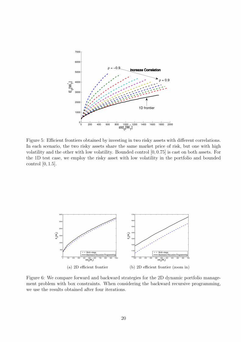
First, we test the influence of adding another risky asset to the portfolio. Here wesimply implement the multi-stage strategy for generating the mean-variance efficient fron-tier. As shown in Figure 5, increasing diversification in the portfolio has a significantimpact on the solution of the dynamic optimization problem. When the correlationbetween the two risky assets is close to −1, an optimal efficient frontier can be ob-tained. This is intuitive, because a large part of the volatility can be hedged in thecase of two negatively correlated risky assets. When their correlation gets larger, theefficient frontier gets worse. However, in most cases two risky assets in the portfolioyield better results than having one risky asset in the portfolio. For example, when wechoose the correlation to be 0.4 and the final target to be 5856.15, as used in Section6.1.2, we obtain [E0[W ∗T ], Std0[W ∗T ]] = [2501.41, 893.87] which is significantly better than[E0[W ∗T ],Std0[W ∗T ]] = [2031.65, 987.55] as acquired in the 1D case.
In Figure 6, we compare the multi-stage strategy and the backward recursive pro-gramming approach. The outcome is similar to that observed in the 1D tests. When weimplement the backward recursive programming stage, a significant improvement is ob-tained. For example, when the standard deviation is around 200, an almost 10% higherexpected return can be obtained if we consider the backward recursive programmingapproach rather than the multi-stage approach.
Remark 6.1. In the 2D case, we also observe that satisfactory results can be obtainedafter several iterations of backward recursive programming even if we start with an inac-curate initial guess of the asset allocations.
7 Conclusion
In this paper, we propose simulation-based approaches for solving the dynamic mean-variance portfolio management problem. To deal with the nonlinearity of the conditionalvariance, we use the embedding technique introduced in [LN00] to transform the mean-variance optimization problem into a linear-quadratic problem, which has a determinedfinal optimization target. To tackle this target-based dynamic optimization problem, alsoknown as “the pre-commitment problem”, we propose two approaches, one in a forwardfashion and the other in a backward fashion.
8First, we solve the unconstrained 2D problem. Then we penalize the optimal solution when the constraintsare not satisfied.
19
0 200 400 600 800 1000 1200 1400 1600 1800 20000
1000
2000
3000
4000
5000
6000
7000
ρ = −0.9Increase CorrelationIncrease CorrelationIncrease CorrelationIncrease CorrelationIncrease CorrelationIncrease CorrelationIncrease CorrelationIncrease CorrelationIncrease Correlation
ρ = 0.9
Increase Correlation
std0[W
*
T]
E0[W
* T]
1D frontier
Figure 5: Efficient frontiers obtained by investing in two risky assets with different correlations.In each scenario, the two risky assets share the same market price of risk, but one with highvolatility and the other with low volatility. Bounded control [0, 0.75] is cast on both assets. Forthe 1D test case, we employ the risky asset with low volatility in the portfolio and boundedcontrol [0, 1.5].
0 100 200 300 400 500 600 700 800 900 10000
500
1000
1500
2000
2500
3000
std0[W
*
T]
E0[W
* T]
Multi−stage
Backward Recursive Programming
(a) 2D efficient frontier
200 220 240 260 280 300 320 340 360 380 4001000
1100
1200
1300
1400
1500
1600
1700
std0[W
*
T]
E0[W
* T]
Multi−stage
Backward Recursive Programming
(b) 2D efficient frontier (zoom in)
Figure 6: We compare forward and backward strategies for the 2D dynamic portfolio manage-ment problem with box constraints. When considering the backward recursive programming,we use the results obtained after four iterations.
20

The forward approach, called the “multi-stage strategy”, is based on determining anintermediate investment target at each re-balancing time. The intermediate target ischosen as the amount of wealth, which, if obtained, an investor can invest with a risk-freestrategy and still reach the final investment target. Although it is generally believed thatbackward programming is essential for solving a dynamic optimization problem, we provethat the multi-stage strategy yields optimal controls when no constraints are involved. Inthe case that there are constraints on the controls, the multi-stage strategy can only yielda sub-optimal solution. However, since it is a forward and thus highly efficient approach,it is always feasible even when the dimensionality of the problem increases.
Although the forward approach is fast and easy-to-implement, in general it is notoptimal for a dynamic optimization problem. Therefore, we propose another simulation-based approach which involves backward recursive programming. The main idea of thebackward recursive approach is that we consider local quadratic optimization insteadof global optimization. By tailoring the numerical algorithm, the backward recursiveprogramming is guaranteed to yield convergent results after several iterations. In thenumerical tests, it is shown that, although the backward approach is also sub-optimal, italways generates better efficient frontiers than the multi-stage strategy.
In the backward approach, we need to calculate conditional expectations associated toeach simulated path recursively by least-squares regression. To make this regression-basednumerical approach stable, we implement “bundling” and the “regress-later” techniques,as introduced in [JO15]. We find that our backward recursive approach is very robust.Even if it is initiated by an inaccurate guess for the allocation, highly satisfactory resultscan be obtained after several iterations.
As both the forward and backward approaches are based on simulation, it is feasibleto implement them for high-dimensional problems. Moreover, since at each single stageor recursive step we consider a constrained quadratic optimization problem, it is possibleto solve them efficiently with suitable quadratic optimization algorithms. Combining thealgorithms with these quadratic optimization algorithms for a general high-dimensionalcase will be our future work. Another research direction is to implement our backwardrecursive programming approach to generate a time-consistent strategy.
References
[BC10] Suleyman Basak and Georgy Chabakauri. Dynamic mean-variance assetallocation. Review of Financial Studies, 23(8):2970–3016, 2010.
[Ber95] Dimitri P Bertsekas. Dynamic programming and optimal control, volume 1.Athena Scientific Belmont, MA, 1995.
[BGSCS05] Michael W Brandt, Amit Goyal, Pedro Santa-Clara, and Jonathan R Stroud.A simulation approach to dynamic portfolio choice with an application tolearning about return predictability. Review of Financial Studies, 18(3):831–873, 2005.
[BJPZ05] Tomasz R Bielecki, Hanqing Jin, Stanley R Pliska, and Xunyu Zhou.Continuous-time mean-variance portfolio selection with bankruptcy prohi-bition. Mathematical Finance, 15(2):213–244, 2005.
[BMOW13] Stephen Boyd, Mark Mueller, Brendan O’Donoghue, and Yang Wang. Per-formance bounds and suboptimal policies for multi-period investment. Foun-dations and Trends in Optimization, 1(1):1–69, 2013.
21
[CGLL14] Xiangyu Cui, Jianjun Gao, Xun Li, and Duan Li. Optimal multi-periodmean-variance policy under no-shorting constraint. European Journal of Op-erational Research, 234(2):459–468, 2014.
[CLWZ12] Xiangyu Cui, Duan Li, Shouyang Wang, and Shushang Zhu. Better than dy-namic mean-variance: Time inconsistency and free cash flow stream. Math-ematical Finance, 22(2):346–378, 2012.
[CO15] Fei Cong and Cornelis W Oosterlee. Accurate and robust numerical methodsfor the dynamic portfolio management problem. Available at SSRN 2563049,2015.
[DF14a] Duy-Minh Dang and Peter A Forsyth. Better than pre-commitment mean-variance portfolio allocation strategies: A semi-self-financing Hamilton-Jacobi-Bellman equation approach. Available at SSRN 2368558, 2014.
[DF14b] Duy-Minh Dang and Peter A Forsyth. Continuous time mean-variance opti-mal portfolio allocation under jump diffusion: An numerical impulse controlapproach. Numerical Methods for Partial Differential Equations, 30(2):664–698, 2014.
[FLLL10] Chenpeng Fu, Ali Lari-Lavassani, and Xun Li. Dynamic mean-variance port-folio selection with borrowing constraint. European Journal of OperationalResearch, 200(1):312–319, 2010.
[FV14] Peter A Forsyth and Kenneth R Vetzal. Long term asset allocation for thepatient investor. 2014.
[GHV04] Russell Gerrard, Steven Haberman, and Elena Vigna. Optimal investmentchoices post-retirement in a defined contribution pension scheme. Insurance:Mathematics and Economics, 35(2):321–342, 2004.
[GHV06] Russell Gerrard, Steven Haberman, and Elena Vigna. The management ofdecumulation risks in a defined contribution pension plan. North AmericanActuarial Journal, 10(1):84–110, 2006.
[HV02] Steven Haberman and Elena Vigna. Optimal investment strategies and riskmeasures in defined contribution pension schemes. Insurance: Mathematicsand Economics, 31(1):35–69, 2002.
[JM70] David H Jacobson and David Q Mayne. Differential dynamic programming.American Elsevier Pub. Co., 1970.
[JO15] Shashi Jain and Cornelis W Oosterlee. The stochastic grid bundling method:Efficient pricing of Bermudan options and their Greeks. Applied Mathematicsand Computation, 269(1):412–431, 2015.
[LN00] Duan Li and Wan-Lung Ng. Optimal dynamic portfolio selection: Multi-period mean-variance formulation. Mathematical Finance, 10(3):387–406,2000.
[LZL02] Xun Li, Xunyu Zhou, and Andrew EB Lim. Dynamic mean-variance port-folio selection with no-shorting constraints. SIAM Journal on Control andOptimization, 40(5):1540–1555, 2002.
[Mar52] Harry M Markowitz. Portfolio selection. The Journal of Finance, 7(1):77–91,1952.
[MF15] Kai Ma and Peter A Forsyth. Numerical solution of the Hamilton-Jacobi-Bellman formulation for continuous time mean variance asset allocation un-der stochastic volatility. Journal of Computational Finance, Forthcoming,2015.
22
[SB08] Joelle Skaf and Stephen Boyd. Multi-period portfolio optimization with con-straints and transaction costs. Technical report, Citeseer, 2008.
[TES08] Yuval Tassa, Tom Erez, and William D Smart. Receding horizon differen-tial dynamic programming. In Advances in neural information processingsystems, pages 1465–1472, 2008.
[WF10] Jian Wang and Peter A Forsyth. Numerical solution of the Hamilton-Jacobi-Bellman formulation for continuous time mean variance asset allocation.Journal of Economic Dynamics and Control, 34(2):207–230, 2010.
[WF11] Jian Wang and Peter A Forsyth. Continuous time mean variance asset alloca-tion: A time-consistent strategy. European Journal of Operational Research,209(2):184–201, 2011.
[WF12] Jian Wang and Peter A Forsyth. Comparison of mean variance like strategiesfor optimal asset allocation problems. International Journal of Theoreticaland Applied Finance, 15(02), 2012.
[ZL00] Xunyu Zhou and Duan Li. Continuous-time mean-variance portfolio selec-tion: A stochastic LQ framework. Applied Mathematics & Optimization,42(1):19–33, 2000.
23