HAL Id: hal-02651214https://hal.archives-ouvertes.fr/hal-02651214

Submitted on 29 May 2020

HAL is a multi-disciplinary open accessarchive for the deposit and dissemination of sci-entific research documents, whether they are pub-lished or not. The documents may come fromteaching and research institutions in France orabroad, or from public or private research centers.

L’archive ouverte pluridisciplinaire HAL, estdestinée au dépôt et à la diffusion de documentsscientifiques de niveau recherche, publiés ou non,émanant des établissements d’enseignement et derecherche français ou étrangers, des laboratoirespublics ou privés.

Multi-element analysis of plant and soil samplesS. Ayrault

To cite this version:S. Ayrault. Multi-element analysis of plant and soil samples. Trace and Ultratrace Elements in Plantsand Soils, 2005. �hal-02651214�

Multi-element analysis of plant and soil

samples

S. Ayrault Laboratoire Pierre Süe, CEA-CNRS, France

Abstract

This chapter is dedicated to the application of six methods of trace element

analysis to environmental studies: Instrumental Neutron Activation Analysis

(INAA), Synchrotron X-ray Fluorescence (SXRF), Proton Induced X-ray

Emission (PIXE), Atomic Absorption Spectrometry (AAS), Inductively Coupled

Plasma - Atomic Emission Spectrometry (ICP-AES), Inductively Coupled

Plasma - Mass Spectrometry (ICP-MS). These methods are categorised into (i)

direct techniques, and (ii) destructive techniques. INAA, SXRF and PIXE belong

to the first category, while AAS, ICP-AES and ICP-MS are destructive methods.

The advantages and disadvantages of each method for a particular application are

described. The detection limits are given in the cases of soil and/or plants

analysis. The comparison of methods on their optimal detection limits, usually

provided by manufacturers, is not correct. In this chapter, the practical point of

view is privileged. An emphasis is put on the definition of the problem before

choosing the method and on the data evaluation. Means of defining the analytical

problem to choose the most convenient analytical procedure and of evaluating the

data are proposed.

1 Introduction

In this chapter, six different techniques to determine trace elements in plants and

soils will be described.

In order of appearance:

Instrumental Neutron Activation Analysis (INAA)

Synchrotron X-ray Fluorescence (SXRF)

Proton Induced X-ray Emission (PIXE)

Atomic Absorption Spectrometry (AAS)

Inductively Coupled Plasma - Atomic Emission Spectrometry (ICP-AES)

Inductively Coupled Plasma - Mass Spectrometry (ICP-MS) They are among the most used environmental analytical techniques, but the

world of environmental analysis is not restricted to these six methods. Three of

the six methods described here are direct methods: the samples can be analysed

in their natural state. The AAS, ICP-MS and ICP-AES are destructive methods

that imply, in the case of these solid samples, digestion and dissolution

processes. Each method has its own capabilities in terms of range of elements

and detection limits. But all of them are able to measure elements at trace level.

The aim of this description is not to be exhaustive about each method, but to give

a clear idea of their potential use in environmental studies.

To illustrate the trace analysis at ppb level, let us take a rather practical

example (Fig 1). Mix one milligram of salt with one ton of coal. Mix it well.

Grind the coal and take one hundred milligrams of this powder. In this aliquot,

the trace of the salt grain (equivalent to 1.10-12 gram) will be found.

Figure 1: Trace analysis at ppb (ng.g-1) level.

The incorrect use of the modern, powerful methods of trace analysis results in

a “data cemetery” mentioned by Markert [1]. When these false data are not used,

the cost of such errors is high, because all of these methods are rather expensive

to buy and use. When they are used, they lead to misinterpretation of elements in

the environment, and can impact on political decisions.

2 Formulating the question

Before undertaking an environmental study, implying the use of financial and

human means, the problem has to be clearly stated. This is not only true for

environmental studies. Several questions have to be addressed to define the

overall analytical procedure that will be the most convenient.

The first question is the matrix. What samples will be analysed? The nature of

the samples (its matrix) and the number of samples to analyse will partly define

Determination

the analytical procedure.

The second question is the number of elements to determine. Only one? Or a

wide range?

The third question is the sensitivity required. In the case of several “trace

elements” to be determined, the range of concentrations to explore is large. In

plants, the concentration levels may vary from less than one microgram per

kilogram (e.g. Sc) to hundreds milligrams per kilogram (e.g. Zn). In Table 1, the

concentration may vary over one or more orders of magnitude for a given

element. The As median value is 0.2 mg/kg, but the minimum value is 0.04

mg/kg and maximum value is 3.1 mg/kg. Literature data (Table 2) and target

concentrations for a good quality soil (Vegter [2]) can be used to evaluate the

levels of concentrations for an element that will be determined in soils. The trace

element contents of soils are higher by a factor of 10 than in plants.

The last question is the accuracy level needed for the study, taking into

account that the turnover of the procedure and the level of accuracy are usually

opposites.

If speciation information is requested, special sampling strategies are required

(Markert [3]). In this case, some recommendations could be false. Speciation is a

specific area, and will not be discussed here.

3 The steps of the analysis and associated errors

From the definition of the problem to the evaluation of the results, all the steps

have their own error potential (Fig 2). Among all the steps of the study, the

analytical step is not the more fragile.

The sample preparation consists of several physicochemical procedures

through which the field samples will become analysed samples: Sampling

Cleaning

Drying, homogenisation and storage

Each of these steps is a potential error source. Time-consuming, they have to

be designed in relation with the problem. During preparation, the main error

source is the contamination. This risk increases exponentially when the element

concentration decreases. When handling the samples, one has to keep in mind

that the goal of all this work is to measure very low concentrations. The

cleanliness of the working area and the tools used as well as the reagents used to

clean them has to be a constant preoccupation. The contamination risk has to be

eliminated at all stages of the sample handling. White paper may contain

whiteners made of metal oxides and marker pen inks may contain heavy metals.

Cleaning, drying and homogenisation of plant matrices have been described

by Markert [5]. Sampling may be considered as a source of measurement

uncertainty. Techniques for quantification and comparison with analytical

sources have been proposed (Ramsey [6]).

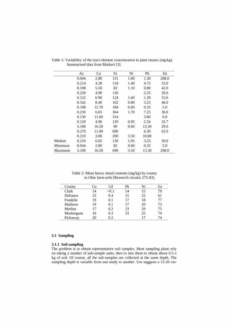
Table 1: Variability of the trace element concentration in plant tissues (mg/kg).

Summarised data from Markert [3].

As Cu Fe Ni Pb Zn

0.044 2.80 131 1.00 1.30 208.0

0.214 4.28 118 1.40 4.75 53.0

0.108 5.50 82 1.10 0.80 42.0

0.220 4.90 130 2.25 20.0

0.122 6.90 124 1.60 1.29 53.6

0.542 8.40 102 0.80 3.25 46.0

0.198 12.70 184 0.60 0.35 5.0

0.230 6.65 364 1.70 7.25 36.0

0.150 11.60 314 3.80 6.0

0.120 4.90 120 0.95 2.54 32.7

3.100 16.50 90 0.60 13.30 29.0

0.270 11.00 690 6.30 62.0

0.210 3.00 200 3.50 10.80

Median 0.210 6.65 130 1.05 3.25 39.0

Minimum 0.044 2.80 82 0.60 0.35 5.0

Maximum 3.100 16.50 690 3.50 13.30 208.0

Table 2: Mean heavy metal contents (mg/kg) by county

in Ohio farm soils [Research circular 275-83].

County Cu Cd Pb Ni Zn

Clark 14 <0.1 14 15 79

Defiance 23 0.4 15 22 61

Franklin 19 0.1 17 18 77

Madison 19 0.1 17 20 73

Medina 17 0.2 23 20 75

Muskingum 16 0.3 33 25 74

Pickaway 20 0.2 17 74

3.1 Sampling

3.1.1 Soil sampling

The problem is to obtain representative soil samples. Most sampling plans rely

on taking a number of sub-sample units, then to mix them to obtain about 0.5-1

kg of soil. Of course, all the sub-samples are collected at the same depth. The

sampling depth is variable from one study to another. Ure suggests a 15-20 cm-

depth for arable soil and 7.5-10 cm for grassland (Ure [7]). Stainless steel, PVC

(polyvinylchloride) and rusty tools have to be avoided. Aluminium and PTFE

(polytetrafluoroethylene, Teflon®) are recommended. The soil is then put in a

polyethylene bag or box, labelled outside with a permanent mark.

Figure 2: Simplified flow chart for the instrumental multi-element analysis

of environmental samples. From Markert [1], with permission.

Analytical steps Estimation of errors

Defining the scientific problem

Discussion by experts

Benefit / Use of calculation

Planning of analysis

Representative sampling

Sample preparation

I. Physical

washing

drying

homogenization

II. Chemical

ashing

decomposition

enrichment

speciation

Instrumental measurement

Data evaluation

Solving the scientific problem

Production of

‘data cemetery’

Up to 100%

Between 100

and 300%

Normally between

2 and 20%

Up to 50%

Analytical steps Estimation of errors

Defining the scientific problem

Discussion by experts

Benefit / Use of calculation

Planning of analysis

Representative sampling

Sample preparation

I. Physical

washing

drying

homogenization

II. Chemical

ashing

decomposition

enrichment

speciation

Instrumental measurement

Data evaluation

Solving the scientific problem

Production of

‘data cemetery’

Up to 100%

Between 100

and 300%

Normally between

2 and 20%

Up to 50%

3.1.2 Plant sampling

For plants sampled in the field, the species determination is a hard point. An

Italian study on lichen biodiversity showed that, if the quantitative data were

satisfactory, the taxonomic assignment was less than 50 % on average (Brunalti

et al [8]).

To avoid contamination during sampling, the use of powder-free gloves is

recommended. When cutting is necessary, the use of ceramic scissors is

necessary (such scissors are available from Kyocera®).

But many others factors can affect the bioconcentration: climatic conditions,

seasonal variations, and age of the plant. The heterogeneity of the trace element

content in between the different parts of the plants (roots, leaves - old and young,

seeds…) has to be taken into account.

If the samples can not be prepared immediately, they should be stored in a

fridge (4°C) in polyethylene bags or boxes.

3.2 Cleaning

For soils, this question is solved by sieving after air drying at ambient

temperature (Ure [7]) with a 2-mm aluminium sieve.

For plants, it depends on the specific problem of the study. In the case of

atmospheric fall-out study, the samples must not be cleaned. But in the case of

soil-to-plant transfer, the surface contamination may interfere with the results.

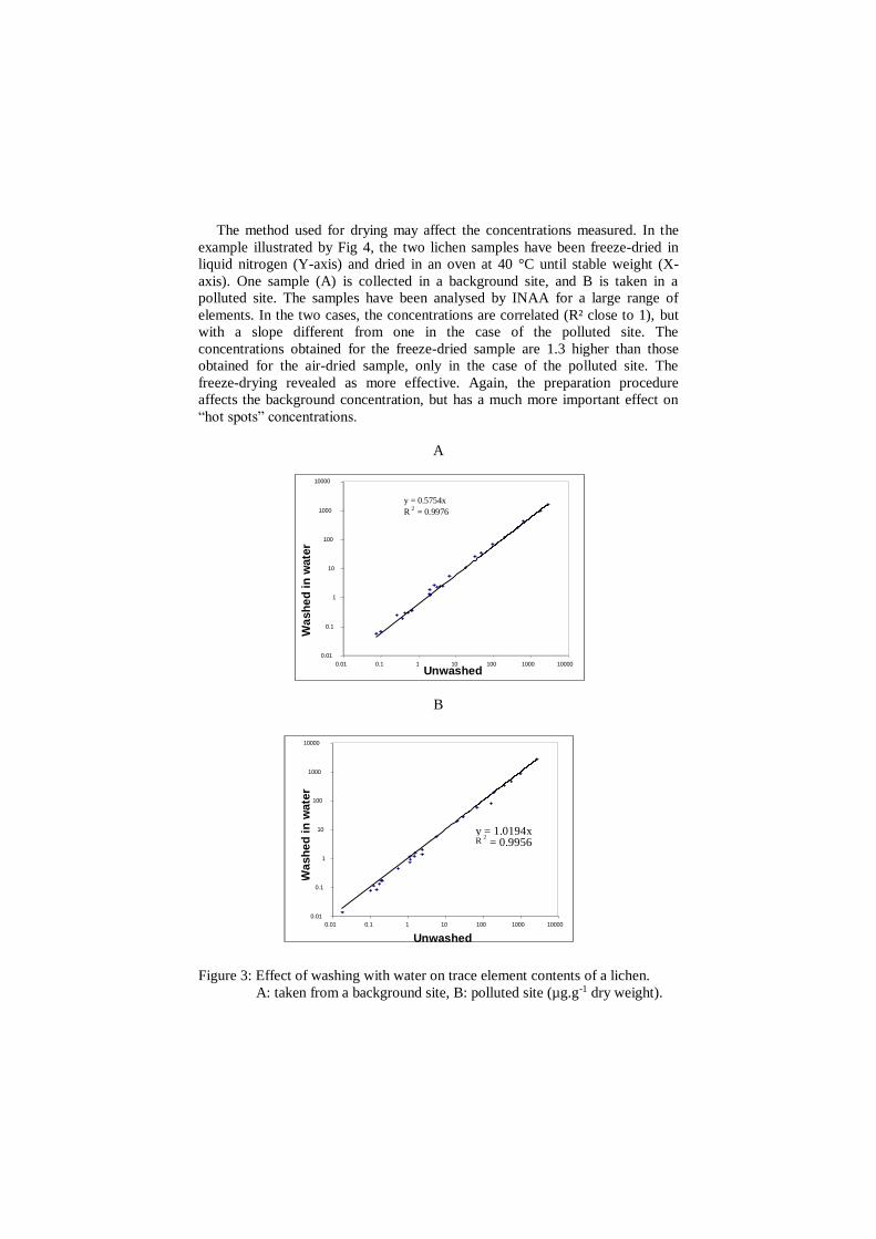
The effect of washing with water on trace element content is illustrated by

Fig 3. Two lichen samples, taken in a background site (A) and in a polluted site

(B), have been divided into two subsamples. One is immersed in bi-distilled

water. The samples have been analysed by INAA for a wide range of elements

and the results (µg.g-1) compared. If the washing results in no effect for the less

polluted site, the content of the lichen collected from the polluted area is greatly

affected. Forty percent of the content are lost.

To remove the outer wax layer of some vegetable samples (e.g. pine needles),

Wyttenbach and Tobler [9] recommended washing thoroughly the samples. This

treatment allows obtaining intrinsic (biologically active) concentrations. The

fluid used for washing is a mixture of tetrahydrofurane and toluol. This drastic

procedure will damage the cell walls and has to be strictly reserved to waxy

plants.

3.3 Drying, homogenisation and storage

3.3.1 Plants

To avoid losses of volatile compounds (e.g. arsenic species), a temperature lower

than 80°C is recommended. Temperatures of 40°C and 65°C are currently used,

for duration approx. 24 hours, to reach a stable weight. For mercury analysis, the

samples are analysed without drying or freeze-dried (Sloan et al [10]). When the

samples are analysed without drying, the analytical results are reported to the dry

weight. The dry/wet ratio is measured using separate fractions of the samples.

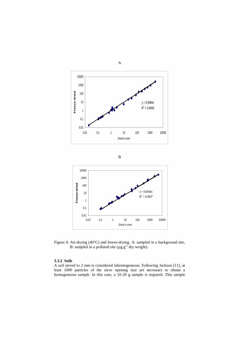
The method used for drying may affect the concentrations measured. In the

example illustrated by Fig 4, the two lichen samples have been freeze-dried in

liquid nitrogen (Y-axis) and dried in an oven at 40 °C until stable weight (X-

axis). One sample (A) is collected in a background site, and B is taken in a

polluted site. The samples have been analysed by INAA for a large range of

elements. In the two cases, the concentrations are correlated (R² close to 1), but

with a slope different from one in the case of the polluted site. The

concentrations obtained for the freeze-dried sample are 1.3 higher than those

obtained for the air-dried sample, only in the case of the polluted site. The

freeze-drying revealed as more effective. Again, the preparation procedure

affects the background concentration, but has a much more important effect on

“hot spots” concentrations.

A

B

Figure 3: Effect of washing with water on trace element contents of a lichen.

A: taken from a background site, B: polluted site (µg.g-1 dry weight).

y = 1.0194xR

2

= 0.9956

0.01

0.1

1

10

100

1000

10000

0.01 0.1 1 10 100 1000 10000

Unwashed

Wa

sh

ed

in

wate

r

y = 0.5754x

R2 = 0.9976

0.01

0.1

1

10

100

1000

10000

0.01 0.1 1 10 100 1000 10000

Unwashed

Wa

sh

ed

in

wate

r

A

y = 0,9994x

R2 = 0,9945

0,01

0,1

1

10

100

1000

10000

0,01 0,1 1 10 100 1000 10000

Dried in oven

Freeze-d

rie

d

B

Figure 4: Air-drying (40°C) and freeze-drying. A: sampled in a background site,

B: sampled in a polluted site (µg.g-1 dry weight).

3.3.2 Soils

A soil sieved to 2 mm is considered inhomogeneous. Following Jackson [11], at

least 1000 particles of the sieve opening size are necessary to obtain a

homogeneous sample. In this case, a 10-20 g sample is required. This sample

y = 0,6044x

R2 = 0,9847

0,01

0,1

1

10

100

1000

10000

0,01 0,1 1 10 100 1000 10000

Dried in oven

Fre

eze

-drie

d

size is often too large for the analysis. If a dissolution is used, a finely ground

soil is required. Such finely ground soils are prepared by grinding in non-

metallic mortar. The powder is then stored in a dark, cool place. The soil has to

be shaken before sub-sampling for analysis.

4 Trace element determination

Analytical techniques are commonly categorised into two schemes:

(i) single / multi-element techniques

(ii) wet / dry techniques

Both samples under interest, plants and soils, are solid samples. The second

categorisation will be further used.

The principle of the analytical methods will be described briefly. For further

insight, handbooks are recommended for each method.

4.1 Direct measurements

Several methods allow the determination of trace elements without any special

digestion of solid samples. Three of them are described in following text.

Instrumental Neutron Activation Analysis (INAA)

Synchrotron X-ray Fluorescence (SXRF)

Proton Induced X-ray Emission (PIXE)

4.1.1 Sample preparation

To analyse plant and soil samples with non-destructive methods, these samples

have to be dried and homogenised. Usually 100 to 500 mg should be taken for

analysis. Smaller amounts can be analysed, if the sample homogeneity is

demonstrated.

4.1.2 Methods

4.1.1.1 Instrumental neutron activation analysis INAA allows the

determination of trace elements at very low levels. The principle of this method

is the production of radioactive isotopes in a neutron flux.

General reviews on neutron activation analysis can be found in De Soete et al

[12], Kruger [13] and Alfassi [14]. For direct gamma spectrometry of

radionuclides occurring in the environment due to nuclear weapons tests and

accidental situations (e.g. 137Cs), the Practical Gamma-ray Spectrometry

handbook of Gilmore and Hemingway is useful [15].

INAA has several advantages. Among them, its reliability makes INAA the

reference method for solid samples analysis. But INAA suffers from the

drawbacks common to nuclear techniques. To benefit from all the potential of

INAA, a nuclear reactor is necessary.

Due to the penetration of the neutron and the energy of the monitored gamma

emission, the sample irradiated is totally analysed. This idea has to be corrected

if high volume samples are analysed. Because of radiolysis, the irradiation of

humid samples is prohibited. The detection limits and range of elements depend

on available neutron fluxes and background due to major elements. Alternative

reactions and isotopes can be used to obtain better detection limits and more

accurate determination, but only if the convenient fluxes are available.

The Table 3 gives an example of available fluxes in a laboratory provided

with access to two experimental reactors. This situation allows numerous

experimental conditions, and thus covers a wide range of elements and matrixes.

Table 3: Neutron irradiation facilities at the Pierre Süe Laboratory,

CEA Saclay, France (n.cm-2.s-1).

Nuclear Reactor OSIRIS (70 MW) ORPHEE (14 MW)

Channel H1 H2 P1 and P2 P3 P4

Thermal

neutrons

(E = 0.025 eV)

0.77 1014 1.2 1014 1.23 1013 1.65 1013 2.5 1013

Epithermal

neutrons

(E > 0.1 eV)

1.9 1012 4 1012 6.15 109 8.25 109 4.5 1010

Fast neutrons

(E > 0.5 MeV) 9.6 1012 2.3 1013 3.5 109 8.2 109 1.2 1010

The practical devices available in the INAA laboratory impact on the

performance of the method. For example, the determination of selenium using

short-live isotopes is possible if only the decreasing time between irradiation and

gamma counting does not exceed 30 seconds. If such a facility is not available,

selenium determination can be done using a long-life isotope, but its gamma ray

is interfered with U. In this case, the detection limits are not so low.

Economic and political reasons may reduce the access to such facilities.

Another drawback is that the half-life of radioisotopes cannot be changed. A

multi-element analysis may require successive irradiation and counting times.

The INAA turnover is sometimes considered too low for large numbers of

samples. Also, the discontinued availability of nuclear reactors may result in

missing data (Schleppi et al [16]).

The Slowpoke and MSN reactors (Kay et al [17], Ryan et al [18], Kennedy et

al [19]), that are easier to use, cheaper to install and allowing higher turnover,

may be a good alternative to classical experimental reactors. In theory, the

detection limits of the Slowpoke technique are lower than those reached with

classical reactors, due to lower neutron fluxes. This implies the analysis of larger

samples, and limits its interest for very small samples. Nevertheless, this

technique is widely used for environmental survey study(Siddiqui et al [20],

Normandin et al [21], St-Pierre and Kennedy [22], Lin et al [23]).

It is also possible to use nonreactor neutron sources, but they are so lacking in

intensity that they may be used only for determination of major elements. An

alternative source is the neutron generator that, by the deuteron excitation of a

tritium target, produces 14 MeV neutrons from the H(d,n)He reaction. Because

of its characteristic, the neutron generator is more suitable for low atomic

number elements determination. It could be a good complement to classical

NAA (Senhou et al [24]).

The development of high-resolution germanium detectors for -spectrometry

has made possible a complex mixture of -emitters, but it has been recognised

that a purification step is sometimes required. Radiochemical procedures, called

radiochemical neutron activation analysis RNAA, of environmental samples

have been reviewed by Pietra et al. [25]. In this work, 32 separation schemes are

described for groups of elements (up to 50 elements) and single elements.

To separate the element from the interfering -emitters, the analyst can choose

among several procedures, keeping in mind that the radioisotopes have the same

chemical behaviour as the stable isotopes. Thus, liquid-liquid extraction,

precipitation and ion exchange are possible separation techniques. To avoid the

specific problems of manipulating trace amounts (e.g. sorption on glassware or

colloids), a macro-amount of stable isotope, the chemical carrier, can be added,

providing the stable and radioactive isotopes are in the same valence state and

uniformly mixed. To complete this last requirement, the sample passes through

an oxidation-reduction cycle.

Applications of INAA and RNAA to environmental studies are numerous and

can be found, in particular, in the Nuclear Analytical Methods in Life Science

conference proceedings (NAMLS) and in the Journal of Radioanalytical Nuclear

Chemistry.

4.1.1.2 Synchrotron X-ray fluorescence The principle of SXRF technique is to

produce X-ray emission with an X-ray beam issued from a synchrotron. This

capability brought about by the use of a synchrotron source to perform XRF

analysis has been evaluated in the mid 1970s (Sparks [26]). Applications of

synchrotron radiation in environmental sciences have been recently reviewed

(Fenter et al [27]).

During irradiation, an inner shell electron is ejected, thereby creating a

vacancy. A higher energy electron drops onto the lower energy orbital and

releases a fluorescent X-ray. The emitted X-rays are detected by a Si(Li)

detector. The released energy is characteristic of the emitted element. The

intensity of the fluorescent X-ray peak is proportional to the number of atoms of

the element in the samples. The concentrations are determined through

comparison with a standard. The elements with atomic number higher than 14

(Na) are commonly determined by SXRF.

The analysed area is reduced to the beam size. The beam size varies from one

to one hundred micrometers, depending on line and synchrotron technologies.

The scrutinised depth depends on the X-ray penetration in the matrix under

analysis. For example, a leaf is completely analysed, but not a 1 mm-thick pellet

of soil.

SXRF operates at ambient pressure, and microscopic beams are available.

This allows the measurement of the metal content along a plant shoot (Amblard-

Gross et al [28]. The non-destructive characteristic of SXRF is inversely

proportional to the quantity of energy deposed during irradiation. The 3rd

generation synchrotrons (e.g. European Synchrotron Research Facility,

Grenoble, France and ALS, Berkeley, CA) provide energetic beams, and thus

give access to high sensitivity, but the damage to plant cells is no more

negligible.

Synchrotron X-ray microfluorescence can be used in combination with

microdiffraction, and microabsorption spectrometry in characterising the

distribution and the speciation of metals in soils (Juillot et al [29]) and plants

(Sarret et al [30]).

4.1.1.3 Proton induced X-ray emission Proton induced X-ray emission or

PIXE became popular as an analytic tool in the nuclear physic laboratories in the

mid 1970s. General reviews on PIXE can be found in Johansson et al [31] and

Cohen and Clayton [32]. The analysis of biological samples with charged

particle accelerators has been described by Yagi [33]. Proton induced X-ray

emission is based on the fact that irradiation of a material with protons or other

charged particles of a few megaelectron volts per nucleon gives an emission of

characteristic X-rays of the present elements (Fig 5). These X-rays are usually

detected by using a solid-state detector such as Si(Li) detector, and the spectrum

can provide both qualitative and quantitative information.

Application of PIXE analysis to the environmental studies may be

characterised by the following advantages and disadvantages.

Figure 5: Scheme of the analysis of a leaf using the PIXE technique.

X-ray

emission

Incoming

ion beam

Advantages:

PIXE analysis is multielemental and mostly insensitive to the chemical

state of the element.

Elements with atomic number between 13 (Al) and 92 (U) can be

determined in a single run. The sensitivity is fairly constant over this

range.

The theoretical sensitivity is high (between 10-12 and 10-15 g).

The duration of analysis (for punctual determination) is short.

Theoretically, the PIXE analysis is non-destructive.

Very small samples can be analysed.

The PIXE analysis is resolutive in space and thus chemical maps can be

obtained.

Disadvantages:

Interferences can take place between K and L X-rays of light and heavy

elements, and between K and K peaks of neighbouring elements. It may

result in lower performances. This could be overcome by using detectors

with improved resolution.

PIXE analysis is well suited for thin analysis. Thick samples can be

analysed, but the analysis of resulting spectra is considerably complicated

and the accuracy will be reduced.

To illustrate the data that can be obtained with this punctual method, the

chemical maps of five elements in a transversal cut of a lichen thallus are shown

in Fig 6. The correlation between the physiological structure of the lichen and

the partition of elements (e.g. Cl in the algae layer) is clearly demonstrated.

4.2 Destructive methods

Some techniques offer low detection limits but a digestion step prior to the

measurement is necessary.

Three of the most commonly used destructive techniques are described here: Atomic Absorption Spectrometry (AAS)

Inductively Coupled Plasma - Atomic Emission Spectrometry (ICP-AES)

Inductively Coupled Plasma - Mass Spectrometry (ICP-MS).

4.2.1 Sample preparation

Plant and soil samples have to be digested prior to analysis. Different digestion

techniques are available: drying ashing, acid digestion, assisted or not by

microwave. The latter, microwave assisted digestion, is the most commonly used

in laboratory.

Because uncompleted digestion, losses and contamination can affect the

accuracy of the final results, the digestion procedures are widely discussed in

literature (Wu et al [34], Roduskin et al [35], Pöykiö et al [36]). There are a

number of possible mechanisms during digestion that may result in loss of

elements, including volatilisation, adsorption onto surfaces, precipitation and

persistence of non dissolved compounds. In some cases, certain reagents can not

be used because they would produce interfering compounds. For ICP-MS

technique (see below for description), nitric media are preferred. Many studies

have reported good recoveries in various biological matrixes by using

concentrated HNO3 at an elevated temperature and pressure. Addition of H2O2

enhances the digestion of the organic matrix, but this procedure is still not

powerful enough to dissolve siliceous materials. Addition of HF may be needed.

The reagents added directly influence the final detection limits. The adopted

digestion procedure is a compromise between low detection limits and

achievement of the digestion.

Figure 6: Maps of K, Ca, Cl, Fe and Pb in a section of lichen thallus. The higher

concentrations are shown with white and black dashes for major and

minor elements (Ca, K, Fe, Cl) and trace element (Pb), respectively.

These maps were obtained at Laboratory Pierre Süe microprobe, CEA-

Saclay, France.

K

Cl

Ca

Fe

Pb

The environmental concentrations of some elements of interest (e.g. As, Cd,

Pt) are sometimes very low (less than one nanogram per gram of dry sample).

Instead of the sensitivity of the analytical tools used for the trace elements

determination, it is sometimes necessary to concentrate the element to be

determined to make the determination possible and/or accurate. Preconcentration

by solvent- and ultrasound-assisted extraction have been explored. These

extractions are time-consuming and this fact explains why techniques with better

signal-to-background ratio are still being researched, even if the methods

presented in this chapter attain amazing theoretical detection limits.

One rarely used technique to obtain data on ultra-trace elements is to digest

larger samples. While the analysed sample mass usually does not exceed 500

mg, Niemelä et al [37] digested samples of up to 2 g in a microwave oven to

determine arsenic in mosses.

4.2.2 Methods

4.2.2.1 Atomic Absorption Spectrometry Atomic absorption spectrometry

(AAS) is the older method of the three described here. Cheap and easy to use, it

is still often used in environmental studies. The AAS method has been widely

described (Haswell [38]). The application of AAS to soil analysis has been

discussed by Ure [39].

AAS is a typical mono-element method, with a rather limited dynamic range.

The sensitivity of AAS has been greatly increased by the use of a graphite oven

(GF-AAS). There are several variants of AAS, with the introduction of hydrid

generation (HG -AAS) and cold vapour (CV-AAS) technologies. Among them,

CV-AAS is still the best method to analyse mercury in plants and soils.

Free atoms of an element absorb light at wavelengths characteristic of that

element, and the absorption is a measure of the concentration of these atoms in

the light path. The production of atoms from the sample requires a source of

energy. In the case of AAS, a flame provides the energy. This flame can vaporise

and dissociate the elements into their gaseous state in which the atomic

absorption takes place. The wavelengths of interest are selected by the

monochromator and a photomultiplier produces an output current, proportional

to the incident light intensity. The atomic concentration in the flame is

proportional to the measured absorbance and from this the element concentration

in the sample solution can be found by standardisation.

Five error sources can be listed for AAS: spectral, physical, ionisation,

background and chemical effects. The spectral effects are low. The physical

effects, due to viscosity, presence of solvents or high salt concentrations, can be

overcome by dilution or matrix-matching standard solutions. The ionisation

effects depend on the flame temperature and the ionisation potential of the

element. Addition of an element with low ionisation potential, or decreasing the

flame temperature, reduce the ionisation effects. The background effect is most

pronounced at short wavelengths. The interference arises with the increase of

concentration of major elements in solution. The background effects can be

removed by separating the element from the interfering elements, or

alternatively, by calculating the interference using a non-absorbing line. The

most frequently encountered interference effects in AAS are due to chemical

effects. The formation of refractory compounds with Al, P and Si in the flame

may reduce the absorption of calcium. These effects can be overcome by the

addition of agents such as EDTA.

Limitations to the sensitivity of atomic absorption spectrometry analysis

using flame atomisers (FAAS), and the need to analyse samples too small for

continuous nebulisation, have encouraged the use of electrically heated furnace

atomisers (ETA-AAS, for electrothermal atomisation or GF-AAS, for graphite

furnace). The technique involves pipetting a small volume (1 - 100 µL) into the

furnace where the sample is gradually heated up to 1200°C by passing an electric

current through the furnace material, to atomise the components. All operations

are performed in an inert gas atmosphere, usually argon.

The sensitivity reached by ETA-AAS is better than the sensitivity obtained by

F-AAS (Table 4), but ETA-AAS requires more sophisticated background

correction, since the smoke and molecular species produced during heating are

retained on furnace walls. Reliable analysis can be carried out with some

cautions (L’vov [40]).

4.2.2.2 Inductively coupled plasma - atomic emission spectrometry

Inductively coupled plasma - atomic emission spectrometry (ICP-AES) was

introduced nearly thirty years ago, and has become an advanced and very

popular technique (Montaser and Godlightly [41]). Several authors (Zyrnicki and

Prusisz [42], Hoenig et al [43]) have described applications of ICP-AES to plants

and environmental sample analysis.

The plasma provides the energy necessary for the emission of atomic spectra,

characteristic of the element. The energy required for the emission of atomic

spectra increases as the wavelength decreases. Conventional AAS flames

(air/acetylene and even nitrous oxide/acetylene) are of little values for elements

whose analytical wavelengths are less than 250 nm. In this case, the power of

plasma allows the multielement analysis of solutions. High-energy sources more

readily decompose compounds into their constituent atoms and provide more

complete atomisation. Thus, they reduce the chemical interference. However, the

spectra are more complicated, due to a higher number of lines, and thus

expensive high-resolution spectrometers are required. Spectral interferences in

ICP-AES are more severe than in AAS.

For complex solutions, e.g. dissolved soil solutions, major elements can

introduce large background errors due to high scattered lights levels consequent

on the high intensity emitted by these elements. This background interference

can often be overcome by choosing an alternative line or using a correction

procedure. There are two correction procedures: the blank subtraction (only if the

interfering element concentration is constant from one sample to another) and the

measured contribution of the interfering element. Physical effects due to

viscosity, solvent volatility, can affect sample transport and nebulisation

efficiency. The use of matrix-match standard solutions can overcome these

effects.

Table 4: Detection limits by AAS (from Ure [39] with permission).

Element Detection limit

(µg ml-1 in solution)

Flame a ETA

b

Ag

As

B

Ba

Be

Cd

Co

Cr

Cu

Ga

Ge

Hg

Li

Mn

Mo

Ni

Pb

Rb

Sc

Sn

Sr

Ti

V

Y

Zn

Zr

0.002

0.11

2.0

0.02

0.0007

0.0007

0.007

0.005

0.002

0.038

0.038

0.16

0.0015

0.002

0.03

0.008

0.15

0.002

0.025

0.031

0.002

0.05

0.05

0.11

0.001

1.0

0.000005

0.00006

0.00004

0.000001

0.000004

0.00003

0.000005

0.000008

0.000004

0.00006

0.000025

0.00003

0.00006

0.00001

0.00033

0.00015

0.000001

a: Varian Techtron AA6. Manufacturer’s data.

b: Instrumentation Laboratory 555 Furnace atomiser.

Manufacturer’s data.

4.2.2.3 Inductively coupled plasma - mass spectrometry Inductively coupled

plasma - mass spectrometry (ICP-MS) was “discovered” in 1982 and promptly

arrived in the laboratory. Several types of device are now available. Careful

attention was paid to sample introduction, mass spectrometer, and interference

reduction all over the last decade and ICP-MS changed its status from “very

promising” to a commonly used technique. Several handbooks about ICP-MS

can be recommended (Jarvis et al [44], Montaser [45]). ICP-MS instruments are

commonly designed to analyse liquid samples. A classical quadrupole ICP-MS

apparatus scheme is shown in Fig 7.

Figure 7: Schematic diagram of a quadrupole ICP-MS apparatus.

The liquid is converted to an aerosol. A nebuliser achieves the aerosol

formation. A peristaltic pump at a flow rate usually between 0.5 and 2.0 ml min-1

pumps the liquid sample to the nebuliser. A stream of argon (‘nebuliser gas’)

enters an opening in the bottom of the nebuliser (Fig 8). The sample and argon

both exit the nebuliser through the small orifice at the nebuliser tip. The aerosol

enters the spray chamber. The large droplets collide with the spray chamber

walls and exit through the drain, a plastic tube connected with the peristaltic

pump. The nebuliser gas transports the very fine droplets to the torch. Less than

2 % of the sample solution actually reaches the plasma. The quartz torch consists

of three concentric tubes. The inner tube directs the aerosol to the plasma.

The plasma is formed by coupling the energy from a radiofrequency magnetic

field (1-3 kW power at 27-50 MHz) to free electrons of argon (‘plasma gas’).

The magnetic field is produced from a 2- or 3-turn water-cooled copper coil. The

initial free electrons are provided by a spark Telsa discharge. The electrons are

accelerated by a magnetic field oscillation. The electron collisions allow the

charge transfer. A steady-state plasma is formed while equilibrium between the

production of electrons and the losses by recombination and diffusion is rapidly

reached. A flow of argon (‘cool gas’) protects the torch from fusion and gives to

Argon

Sample

Quadripole

RF Supply

Plasma

TorchIon Lenses

Turbo

Pump

Mech

Pump

Turbo

Pump

Mech

Pump

DetectorComputer

system

Argon

Sample

Quadripole

RF Supply

Plasma

TorchIon Lenses

Turbo

Pump

Mech

Pump

Turbo

Pump

Mech

Pump

DetectorComputer

system

the plasma its doughnut shape. The aerosol brought by the nebuliser gas is

exposed to a temperature of ca. 6000-8000 K for a few milliseconds and the

sequence desolvation-vaporisation-atomisation-excitation takes places in the

plasma.

Figure 8: Scheme of a concentric nebuliser for ICP apparatus.

Once ions are formed in the plasma, they enter the mass spectrometer through

the sampler and skimmer cones. Each cone has a small aperture. The regions

behind the cones are kept at very low pressure. The ions are pumped by the

pressure differential. The cones are usually made of nickel. This may have an

impact on nickel background when the cones become old and used. More

expensive platinum cones are available.

After passing through the cones, the ions are focused into a linear path by a

set of lens. The focused ions enter the mass analyser, which acts as a filter

allowing only ions of one mass to charge ratio to be transmitted at a time to the

detector. All other ions collide with the mass analyser rods. The detector

converts the ion signal into an amplified electron pulse. The detector is protected

from too a high pulse, and the apparatus will promptly change from pulse

counting (PC) mode to analogue mode if the concentration of an element is too

high. The limit between pulse counting and analogue modes is variable from one

apparatus to another. The concentrations that could be measured in PC mode are

higher for light elements (e.g. Be) than for heavy elements (e.g. Pb), and become

lower with the improvements of the technology. This implies an analysis of more

diluted samples than in the past or a careful calibration between PC and analogue

modes.

Solid samples can be analysed via laser ablation (LA-ICP-MS). The problems

due to the use of a laser to sample a solid (homogeneity at micrometer scale,

reproducibility of ablation, calibration standards) are still pertinent for a number

of solids. Applications of LA-ICP-MS for the determination of major, minor and

trace elements in bark samples was described by Narewski et al. [46].

The ICP-MS precision and accuracy, especially for elements of atomic mass

40-80, can be perturbed by interferences due to combinations in the plasma. To

overlap these interferences, the technology of the mass spectrometers was

improved to produce the “high-resolution” apparatus. The potential use of such

Argon

apparatus for plant analysis was promptly tested (Roduskin [47], Townsend

[48]).

ICP-MS analysis can also be used in its semiquantitative mode to obtain a

rapid overview of trace element content in numerous samples (Montès Bayon et

al [49]). This could be useful to get an image of the contamination level over a

large area.

The ability of ICP-MS to analyse small environmental samples was evaluated

using reference materials (Domboravi [50]). Their results showed that, in the

case of very homogeneous samples, it is possible to use amounts as low as 1-5

mg for method development and quality control purposes.

ICP-MS performances depend on the type of apparatus used. Its price remains

high (from 100 kE to 1 ME, depending on the mass spectrometer technology and

accessories), but its ability to determine almost all the elements at very low

concentrations is its great advantage. The apparatus are now “plug and play”,

easy to use and their sample throughput is tremendous. A few minutes are

necessary for each analytical run. Analytical data are thus quickly available. The

main drawback of ICP-MS analysis of plant and soil samples is the preparation

step. As stated above, the digestion is time-consuming and may be the cause of

several analytical errors.

It is interesting to note that the use of a so sophisticated and expensive

technique is contested for soil analysis by some authors (Ure [51]). Few soil

laboratories need so low detection limits and are usually concerned by less than a

dozen elements. The number and costs of reagents used for dissolution as well as

the time required for the preparation reduces the use of this powerful technique

for soil analysis.

5 Choosing the analytical method

The choice of the method should depend on the question to solve. If the problem

is the heavy metals content of a sample, a global method (e.g. INAA, AAS, ICP-

AES or ICP-MS) must be chosen. If the elements of interest are numerous, a

multi-elemental technique is required (e.g. INAA, ICP-AES, ICP-MS). The

behaviour of the sample against digestion is also a matter of choice between

direct and destructive methods.

The sensitivity and accuracy of the methods are also factors of choice. The

elements under interest may also define the method to use. Lead is not attainable

by INAA. Tantalum and hafnium are not easy to solubilise and they are hardly

stable in solution: a direct method could be more adapted to their determination.

Mercury analysis is difficult. CVAAS remains the most sensitive and

reproducible technique for such analysis. On-site techniques have also been

developed to evaluate the quality of a soil (Gerlach et al [52]). When one wants

to know where the leaf accumulates the metals, a punctual method has to be

selected (e.g. SXRF or PIXE). In practice, cost and access may dominate the

choice of the methods.

5.1 Optimal detection limits

The detection limits displayed by handbooks and manufacturers are often

optimal limits. They may be reached only in best conditions (e.g. pure fresh

water for ICP-MS). As stated in 4.1.1.1, INAA detection limits vary with the

facilities. The detection limits displayed in Table 5 were obtained with the

following conditions: neutron flux 1.1014 n.cm-2.s-1, decreasing time not shorter

than 5 minutes, optimised decreasing and counting times. Optimal ICP-MS

detection limits range between ng.L-1 and fg.L-1. The theoretical detection limits

of three destructive methods are compared in Fig 9.

5.2 Detection limits in environmental samples

The real detection limits in environmental samples are often of one to several

order of magnitudes higher, because these samples are often complex. For

destructive methods, a digestion is necessary, followed by dilution to reach a

matrix concentration (e.g. not higher than 2 g.L-1 for ICP-MS analysis of plants).

If soils have to be analysed, the final solution has to be not more than 1 g.L-1, to

avoid clogging. The impurities of the reagents and the contamination due to the

digestion enhance the blank values.

Figure 9: Optimal detection limit ranges of ICP-AES, GF-AAS and ICP-MS.

To compare ICP-MS and INAA detection limits, both methods must be used

to analyse the same samples. Two samples, even very similar (e.g. two plant

species), can behave very differently during digestion.

mg.L-1

ICP-MS

ICP-AES

GF-AAS

ng.L-1 µg.L-1

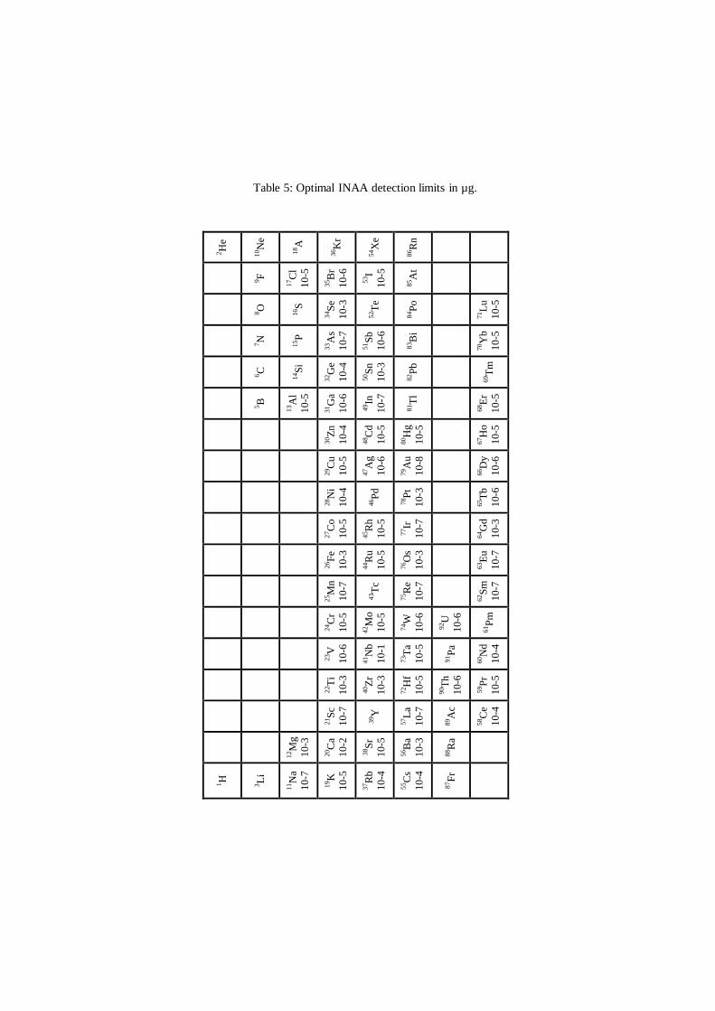
Table 5: Optimal INAA detection limits in µg.

1H

2H

e

3L

i

5B

6C

7N

8O

9F

1

0N

e

1

1N

a

10

-7

12M

g

10

-3

13A

l

10

-5

14S

i 1

5P

1

6S

1

7C

l

10

-5

18A

1

9K

10

-5

20C

a

10

-2

21S

c

10

-7

22T

i

10

-3

23V

10

-6

24C

r

10

-5

25M

n

10

-7

26F

e

10

-3

27C

o

10

-5

28N

i

10

-4

29C

u

10

-5

30Z

n

10

-4

31G

a

10

-6

32G

e

10

-4

33A

s

10

-7

34S

e

10

-3

35B

r

10

-6

36K

r

3

7R

b

10

-4

38S

r

10

-5

39Y

4

0Z

r

10

-3

41N

b

10

-1

42M

o

10

-5

43T

c 4

4R

u

10

-5

45R

h

10

-5

46P

d

47A

g

10

-6

48C

d

10

-5

49In

10

-7

50S

n

10

-3

51S

b

10

-6

52T

e 5

3I

10

-5

54X

e

5

5C

s

10

-4

56B

a

10

-3

57L

a

10

-7

72H

f

10

-5

73T

a

10

-5

74W

10

-6

75R

e

10

-7

76O

s

10

-3

77Ir

10

-7

78P

t

10

-3

79A

u

10

-8

80H

g

10

-5

81T

l 8

2P

b

83B

i 8

4P

o

85A

t 8

6R

n

8

7F

r 8

8R

a 8

9A

c 9

0T

h

10

-6

91P

a 9

2U

10

-6

5

8C

e

10

-4

59P

r

10

-5

60N

d

10

-4

61P

m

62S

m

10

-7

63E

u

10

-7

64G

d

10

-3

65T

b

10

-6

66D

y

10

-6

67H

o

10

-5

68E

r

10

-5

69T

m

70Y

b

10

-5

71L

u

10

-5

The following study-case is issued from the Mosses - Heavy Metals

Deposition program. More than 500 mosses were sampled all over France in

1996 (Galsomiès et al [53]) to participate in a European program (Rülhing and

Steinnes [54]). Each sample was prepared in triplicate. For ICP-MS, the first

aliquot was digested in a microwave oven, with a mixture of HNO3 + H2O2 +

HF. The solution analysed with a quadrupole ICP-MS (Plasma Quad 2+, VG

Elemental) has been diluted to obtain a final concentration of 3.5 g.L-1. This high

concentration is only possible to use in the case of light matrix (plants consisting

mainly of C, H, N, O). The latter aliquots were analysed by INAA. This allowed

the determination of detection limits for 39 elements (Table 6). One can see that

practical detection limits may be very different as compared to theoretical values.

5.3 Comparative evaluation

Keeping in mind the features of the analytical methods, several works stress the

comparative evaluation of the modern analytical techniques for the trace

elements analysis. The first one deals with environmental samples, defined as

water, soil and plant (Table 7) and compares only two techniques: ICP-MS and

INAA. The second column of the table gives the method(s) that can be

reasonably proposed. In the last column, the reasons for the choice of one

method in particular are discussed (Revel and Ayrault [56]). In second example,

the range of environmental samples studied is larger (water, soil, plant and

aerosol). More than five methods are compared (INAA, XRF, ICP-MS, ICP-

AES, electrochemical methods, radiometric method) (Djingova and Kuleff [57]).

Table 8 gives the recommended method for 48 elements.

By comparing these two tables, some conclusions may be drawn. For some

elements, the choice of the “recommended” method is obvious: INAA for Sc,

Au, Hf and Ta. In these cases, the problem due to digestion is the preponderant

criterion. For many other elements, the “sensibility” of the authors may differ. In

practice, the choice of the best method depends on many factors, including range

of elements, expected concentration, accuracy level needed, but also cost, and

availability. It has to be defined in each case. The choice has to be supported by a

quality control investigation, using convenient reference materials.

6 Quality control

To develop a sample preparation process and to validate the data obtained, the

use of certified reference materials is recommended. These materials, named as

CRM, are currently available from several organisations. Three of them are:

National Institute of Standard Technologies (NIST, USA http://ts.nist.gov/srm),

Bureau Communautaire de Référence (BCR, Belgium

http://www.irmm.jrc.be/mrm.html) and International Agency of Atomic Energy

(IAEA, Austria http://www-naweb.iaea.org/nahu/external/e4/nmrm/). These

institutes, and some others, provide a large range of matrixes and elements.

Table 6: Detection limits (µg.g-1 dry weight) in French moss analyses

for ICP-MS and INAA. n.d.: the element was not determined

(Ayrault et al [55]).

INAA ICP-MS INAA ICP-MS

Al 1 - 5 n.d. La 0.01 - 0.07 0.01 - 0.1

As 0.03 - 0.05 0.03 - 0.05 Mg 150 - 200 n.d.

Au 0.0005 - 0.001 n.d. Mn 1 - 5 n.d.

Ba 3 - 14 0.1 - 5 Mo 0.2 - 1 0.01 - 0.08

Bi n.d. 0.05 - 0.08 Na 5 - 10 n.d.

Br 0.03 - 0.1 n.d. Ni n.d. 0.8 - 5.0

Ca 50 - 200 n.d. Pb n.d. 0.1 - 2

Cd 0.2 - 1.0 0.02 - 0.1 Rb 0.3 - 2 0.1 - 0.6

Ce 0.1 - 0.4 0.01 - 0.1 Sb 0.01 - 0.01 0.02 - 0.1

Cl 8 - 13 n.d. Sc 0.001 - 0.006 3 - 5

Co 0.005 - 0.1 0.01 - 0.5 Se 0.1 - 0.5 n.d.

Cr 0.1 - 0.4 0.4 - 1.1 Sm 0.001 - 0.006 0.01 - 0.03

Cs 0.01 - 0.06 0.001 - 0.09 Sr 7 - 24 0.02 - 0.2

Cu 4 - 15 0.2 - 1.7 Th 0.01 - 0.03 0.01 - 0.06

Eu 0.01 - 0.05 0.002 - 0.01 Ti 30 - 70 2 - 10

Fe 10 - 30 10 - 70 U 0.1 - 1 0.003 - 0.02

Hg 0.005 - 0.1 0.03 - 0.07 V 0.2 - 0.8 0.06 - 0.1

I 1 - 10 n.d. W 0.05 - 0.1 0.03 - 0.4

K 50 - 100 n.d. Zn 1.5 - 3 n.d.

Zr 5 - 22 n.d.

It is worth noting that the very first environmental CRM was a cabbage,

prepared by H. J. M Bowen [59] and usually known as the Bowen’s kale. This

cabbage was the first of a long and diversified series of CRM applied to

environmental analytical chemistry. Several certified reference materials now

available and issued from the institutes cited above are listed in Table 9 and

Table 10. Nevertheless, some elements are hardly certified. This is the case for

platinum group elements (PGE) emitted from auto catalysts. Today, no vegetable

CRM is available for PGE (Pt, Pd and Rh) environmental concentrations (ng.g-1).

The use of CRM with matrix and concentration ranges similar to the samples

to be analysed is recommended. In particular, the digestion process performances

may differ strongly from one sample type to another. A soil digestion cannot be

certified using a geological CRM. A soil contains inorganic fractions (sand,

granite, sediments), and organic compounds. All of them have their own

behaviour against digestion and dissolution.

Valuable information about environmental CRM can be found in the

Biological and Environmental Reference Materials (BERM) conference

proceedings.

Table 7: Comparison of INAA and ICP-MS for the determination of elements in

environmental samples. From Revel and Ayrault [56] with permission.

Element Method Comments Li, B, Y,

Nb, Tl, Pb,

Gd, Ho, Er, Tm

ICP-MS NAA not applicable

Mg, Al, Ti,

V, Dy

INAA and ICP-MS Short time irradiation required for INAA

Oxide dissolution (Al2O3) difficult for ICP-MS

Ca INAA and ICP-MS Poor sensitivity by INAA: ray at 1297 keV interferes with the rays of 59Fe, 60Co, 182Ta.

Sc INAA Ca and Ti concentrations conceal Sc concentrations

in ICP-MS. -ray at 889,3 KeV very selective in INAA

Cr, Fe INAA and ICP-MS Oxide dissolution difficult and mass interference for

ICP-MS.

Ni ICP-MS Poor sensitivity using (n,) reaction. Better results obtained by (n,p) reaction which requires a special

irradiation.

Cu ICP-MS Poor sensitivity in INAA. Radiochemical separation

required.

Zn INAA and ICP-MS Blank value difficult to control in ICP-MS

As INAA and ICP-MS Loss risks during the dissolution in ICP-MS. Rb, Th, Ag,

Th, Ce

INAA and ICP-MS

Sr ICP-MS Poor selectivity of 514 keV -ray in INAA Zr INAA Interference risk with uranium fission in INAA

Oxide dissolution (ZrO2) difficult in ICP-MS Mo ICP-MS Interference with uranium fission and poor

sensitivity in INAA

Cd INAA and ICP-MS Poor sensitivity in INAA

Sn ICP-MS Poor sensitivity in INAA Co, Sb, Cs,

Au, Sm, Eu,

Tb, Yb, Lu

INAA and ICP-MS Determination accurate and sensitive by INAA

Ba INAA and ICP-MS Poor selectivity of 496 keV -ray in INAA Hf, Ta INAA Oxide dissolution difficult for ICP-MS W, Pr INAA and ICP-MS INAA not convenient for samples having a high

sodium concentration.

U INAA and ICP-MS Possibility to use delayed neutrons to increase the

INAA sensitivity La INAA and ICP-MS Interference risk with uranium fission in INAA

Nd INAA and ICP-MS Poor selectivity of 531 keV -ray in INAA

Table 8: Recommended methods for determination of selected elements at

background levels in environmental materials. From [57], with

permission.

Element Recommended method Element Recommended method

Al INAAa, ICP-AES, ETAAS,

EDXRF

Na INAA, ICP-AES, EDXRF

As INAA, ICP-MS, HGETAAS,

TXRF

Nd INAA

Au INAA Ni ICP-AES, ETAAS, TXRF

(63Ni- liquid scintilation)

Ba ICP-MS, ICP-AMS, EDXRF,

INAA

P ICP-AES, EDXRF

Br INAA Pb ETAAS, ICP-MS, TXRF

(210Pb- counting)

Ca INAA, ICP-MS, ICP-AES,

ETAAS, FAAS, EDXRF,

TXRF

Pd ETAASc, INAAc

Cd ETAAS Pt ETAASc, INAAc

Ce INAA, ICP-AESb Rb INAA, ICP-MS, ICP-AES,

TXRF, EDXRF

Co INAA, ICP-AES

(60Co- spectrometry)

Sb INAA (125Sb- spectrometry)

Cr INAA, ICP-AES, ETAAS Sc INAA

Cs INAA, TXRF Se ETAAS, INAA

Cu FAAS, ETAAS, ICP-AES,

ICP-MS, TXRF

Si EDXRF

Dy INAAa, ICP-AESb Sm INAA, ICP-AES

Eu INAA, ICP-AESb Sn ETAA, ICP-MS

Fe INAA, ICP-MS, ICP-AES,

ETAAS, FAAS, EDXRF,

TXRF

Sr INAA, ICP-MS, ICP-AES,

ETAAS, FAAS, EDXRF,

TXRF (89-90Sr- counting)

Hf INAA Ta INAA

Hg CVAAS, ICP-MS, INAA Tb INAA, ICP-AESb

K INAA, ICP-MS, ICP-AES,

ETAAS, FAAS, EDXRF,

TXRF

Th INAA, delayed neutron

counting, spectrometry,

spectrometry

La INAA, ICP-AESb, TXRF Ti INAAa, ICP-MS

Li ICP-MS U INAA, delayed neutron

counting, spectrometry,

spectrometry

Lu INAA, ICP-AESb V INAAa, ICP-AES

continued overleaf

Mg INAA, ICP-MS, ICP-AES,

ETAAS, FAAS, EDXRF,

TXRF

Yb INAA, ICP-AESb

Mn INAA, ICP-MS, ICP-AES,

ETAAS, FAAS, EDXRF,

TXRF

(54Mn- spectrometry)

Zn INAA, ICP-MS, ICP-AES,

ETAAS, FAAS, EDXRF,

TXRF

Mo ICP-MS, AAS, TXRF Zr EDXRF

(95Zr- spectrometry) a Short irradiation at the reactor site. b ICP-MS after chemical separation and preconcentration (Markert [58]). c After chemical separation and preconcentrations.

Table 9: Some reference materials for trace element analysis in plant tissues.

Type Species / Variety CRM code Provider

Aquatic plant Lagarosiphon major CRM060 BCR

Lichen Evernia prunastri IAEA-336 IAEA

Lichen CRM482 BCR

Olive leaves Olea europaea CRM062 BCR

Pine needles SRM1575a NIST

Peach leaves Coronet SRM1547 NIST

Sea lettuce Ulva lactuca CRM279 BCR

Tomato leaves SRM1573a NIST

Hay powder CRM129 BCR

Rye grass CRM281 BCR

Cotton cellulose IAEA-V-9 IAEA

Table 10: Some reference materials for trace element analysis of soil.

Type CRM code Provider

San Joaquin soil SRM2709 NIST

Soil containing lead paint SRM2586 NIST

Montana soil SRM2710 NIST

Peruvian soil SRM4355 NIST

Calcareous loam soil BRC141R BCR

Light sandy soil BCR142R BCR

Sewage amended soil BCR143R BCR

Calcareous soil BCR690 BCR

The analyst is now assisted in his work by computers. Among other numerous

advantages, computers allow an easy data release, avoiding reprints errors. But it

is so exciting to draw the first conclusions from the trace element determination

results that sometimes the data check is not complete. The optimisation of the

analytical method by using certified reference materials as described above

displays target values for the CRMs used and blank values. These figures will be

useful for further data control. Before considering data for unknown samples as

final figures, the results must be scrutinised, by comparison with the data bank

constituted during the optimisation process. This implies that CRMs are included

in each series. A checklist of the points to verify can be useful to the analyst:

(1) Check the blank values

(2) Check the CRMs values

(3) Look for data under the detection limits and notify them as ‘<DL’

values

(4) Calculate the median for the series and extract the extreme values

(5) For low values, verify if they cannot be interpreted as ‘<DL’ data

(6) Verify whether high values are real or artefact, and if real, whether

the sample would not contaminate the series.

7 Concluding comments

AAS and ICP techniques are the most used techniques for trace element analysis

in environmental studies. In particular, ICP-MS and its capability for isotopic

analysis showed important potential for improved analytical performance. For

solid sample analysis, the digestion step is still a hard point in environmental

analysis. INAA, that can be considered as a reference method, has a key-role to

play in the development of a new analytical procedure for routine analysis. The

use of certified reference materials is encouraged. In addition to the global

techniques, methods able to determine the elemental location at the micrometer-

scale, like SXRF and PIXE, have proven themselves in the environmental

sample analysis.

References

[1] Markert, B. (ed.). Instrumental element and multielement analysis of plant

samples, Wiley: Chichester, pp. 112-113, 1996a.

[2] Vegter, J. J. Soil protection in the Netherlands. Heavy Metals, Problems and

Solutions, eds. W. Salomons, U. Förstner & P. Mader, Springer: Berlin, pp.

93-95, 1995.

[3] Markert, B. (ed.). Instrumental element and multielement analysis of plant

samples, Wiley: Chichester, pp. 230, 1996b.

[4] Caruso, J. A., Sutton, K. L. & Ackley, K. L. Elemental speciation - New

approaches for trace element analysis, ed. D. Barcelo, Comprehensive

Analytical Chemistry, Wilson & Wilson’s, Elsevier: Amsterdam, 2000.

[5] Markert, B. Quality assurance of plant sampling and storage, Quality

Assurance in Environmental Monitoring - Sampling and Sample

Pretreatment, ed. Ph. Quevauviller, VCH-Publisher: Weinheim, New York,

Tokyo, pp. 215-254, 1995.

[6] Ramsey, M. H. Sampling as a source of measurement uncertainty:

techniques for quantification and comparison with analytical sources, JAAS,

13, pp. 97-104, 1998.

[7] Ure, A. M. Methods for analysis of heavy metals in soils, Heavy Metals in

Soils, 2nd edition, ed. B. J. Alloway, Blackie Academic & Professionnal,

Chapman and Hall: Glasgow, pp. 59-61, 1995.

[8] Brunalti, G., Giordani, P., Isocrono, D. & Loppi, S. Evaluation of data

quality in lichen biomonitoring studies: the Italian experience. Env. Monitor.

Assessment, 75(3), pp. 271-280, 2002.

[9] Wyttenbach, A. & Tobler, L. Effect of surface contamination on results of

plant analysis. Commun. Soil Sci. Plant Anal., 29(7&8), pp. 809-823, 1998.

[10] Sloan, J. J., Dowdy, R. H., Balogh, S. J. & Nater, E. Distribution of mercury

in soil and its concentration in runoff from biosolids amended agricultural

watershed. J. Environ. Qual. 30(6), pp. 2173-2179, 2001.

[11] Jackson, M.L. (ed.) Soil Chemical Analysis, Prentice-Hall: Englewoods

Cliffs, NJ, pp. 30, 1958.

[12] De Soete D., Gijbels, R. & Hoste, J. Neutron Activation Analysis, eds. P.J.

Elving & M. Kolthoff, Wiley-Interscience: London, 1972.

[13] Kruger, P. (ed.), Principle of activation analysis, Wiley-Interscience: New

York, 1971.

[14] Alfassi, Z. (ed.) Activation analysis, 2 v., CRC Press Boca Raton: Fla, 1990.

[15] Gilmore, G. & Hemingway, J (eds.). Practical gamma-ray spectrometry,

John Wiley & Sons, 2002.

[16] Schleppi, P, Tobler, L, Bucher, J. B. & Wyttenbach, A. Multivariate

interpretation of the foliar chemical composition of Norway spruce (Picea

abies). Plant and Soil, 219, pp. 251-262, 2000.

[17] Kay, R.E., Stevens-Guille, P.D., Hilborn J.W. & Jervis R.E. SLOWPOKE:

A new low-cost laboratory reactor. Int. J. Appl. Radiation Isotopes, 24, pp.

509, 1973.

[18] Ryan, D.E., Stuart, D.C. & Chattopadhyay, A. Rapid multielement neutron

activation analysis with a Slowpoke reactor. Analytica Chimica Acta, 100,

pp. 87-93, 1978.

[19] Kennedy G., St-Pierre, J., Wang, K., Zhang, Y., Preston, J., Grant C. &

Vutchkov, M. Activation constants for Slowpoke and MNS reactors

calculated from the neutron spectrum and k0 and Q0 values. J. Radioanal.

Nucl. Chem. 245, pp.167-172, 2000.

[20] Siddiqui M.F.R., Loranger S., Courchesne F., Kennedy G. & Zayed, J.

Manganese contamination in organic soil, bean and oat plants as related to

traffic volume. Bangladesh J. Botany. 30, pp. 43-51, 2001.

[21] Normandin, L., Kennedy, G. & Zayed J. Potential of dandelion (Taraxacum

officinale) as a bioindicator of manganese arising from the use of

metylcyclopentadienyl manganese tricarbonyl in unleaded gasoline. The

Science of the Total Environment, 239, pp. 165-171, 1999.

[22] St-Pierre, J. & Kennedy, G. Effects of Reactor Temperature and Sample

Mass on the Activation of Biological and Geological Materials with a

SLOWPOKE Reactor. Biological Trace Element Research, 7, pp. 481-487,

1999.

[23] Lin, Z.-Q., Schemenauer, R. S., Schuepp, P. H., Barthakur, N. N. &

Kennedy, G.G. Airborne metal pollutants in high elevation forests of

southern Quebec, Canada, and their likely source regions, Agricultural and

Forest Meteorology, 87, pp. 41-54, 1997.

[24] Senhou, A., Chouak, A., Cherkaoui, R. et al. Comparison of NAA-14 MeV,

NAA-k0 and ED-XRF for biomonitoring study in Morocco. J. Radioanal.

Nucl. Chem., 253(2), pp. 247-252, 2002.

[25] Pietra, R., Sabionni, E., Gallorini, M. & Orvini, E. Environmental,

toxicological and biomedical research on trace metals: radiochemical

separations for neutron activation analysis. J. Radioanal. Nucl. Chem. 102,

pp. 69-98, 1986.

[26] Sparks, C.J. Phys. Rev. Lett., 38, pp. 205-208, 1975.

[27] Fenter, P., Rivers, M., Sturchio, N. & Sutton, S. (eds.) Applications of

synchrotron radiation in low-temperature geochemistry and environmental

science. Reviews in Mineralogy & Geochemitry, 49, 2003.

[28] Amblard-Gross, G., Ferard, J. F., Carrot, F., Bonnin-Mosbah, M., Maul, A.,

Ducruet, J. M., Codeville, P., Beguinel, P. & Ayrault, S. Biological fluxes

conversion and SXRF experiment with a new biomonitoring tool for

atmospheric metals and trace element deposition. Environmental Pollution,

120, pp. 47-58, 2002.

[29] Juillot, F., Morin, G., Ildefonse, P., Trainor, T., Benedetti, M., Galoisy, L.,

Calas, G. & Brown Jr, G. Occurrence of Zn/Al hydrotalcite in smelter-

impacted soils from Northern France: Evidence from EXAFS spectrometry

and chemical extractions. Americ. Mineral, 88, pp. 509-526, 2003.

[30] Sarret, G., Saumitou-Laprade, P., Bert, V., Proux, O., Hazemann, J. L.,

Traverse, A., Marcus, M. A. & Manceau, A. Forms of zinc accumulated in

the hyperaccumulator Arabidopsis halleri, Plant Physiology, 130, pp. 1815-

1826, 2002.

[31] Johansson, S. A. E., Campbell, J. L. & Malmqvist, K. G. (eds.) Particle-

Induced X-ray emission spectrometry (PIXE), volume 133 Chemical

Analysis; a Series of Monographs on Analytical Chemistry and its

Application, ed. J. D. Winefordner, John Wiley & Sons: New York, 1995.

[32] Cohen, D. D. & Clayton, E. PIXE, Ion beams for materials analysis, eds. J.

R. Bird & J. R. Williams, Academic Press: New York, 1989.

[33] Yagi, M. Analysis of biological samples with charged particle accelerators.

Elemental Analysis by Particle Accelerators, eds. Z. B. Alfassi & M.

Peisach, CRC Press, pp. 415-447, 1992.

[34] Wu, S., Feng, X & Wittmeier, A. Microwave digestion of plant and grain

reference materials in nitric acid or a mixture of nitric acid and hydrogen

peroxide for the determination of multi-elements by ICP-MS. JAAS, 12, pp.

797-806, 1997.

[35] Roduskin, I., Ruth, T. & Hurrasaari, A. Comparison of two digestion

methods for elemental determinations in plant material by ICP techniques.

Analytica Chimica Acta, 378, pp. 191-200, 1999.

[36] Pöykiö, R., Torvela, H., Perämaki, P., Kuokkanen, T. & Rönkkömaki, H.

Comparison of dissolution methods for multi-element analysis of some plant

materials used as bioindicator of sulphur and heavy metal deposition

determined by ICP-AES and ICP-MS. Analusis, 28, pp. 850-854, 2000.

[37] Niemelä, M., Perämaki, P. & Piispanen, J. Microwave sample-digestion

procedure for determination of arsenic in moss samples using electrothermal

atomic absorption spectrometry and inductively coupled plasma mass

spectrometry. Anal Bioanal Chem, 375, pp. 673-678, 2003.

[38] Haswell, S. J. (ed.) Atomic Absorption Spectrometry, Theory, Design and

Applications, Elsevier, 1991.

[39] Ure, A. M. Atomic absorption and flame emission spectrometry, Soil

Analysis Modern Instrumental Techniques, 2nd edition, ed. K. A. Smith,

Marcel Dekker: New York, pp. 20-21, 1991b.

[40] L’vov, B. V. Electrothermal atomization - the way toward absolute methods

of atomic absorption analysis. Spectrochim. Acta, 33B, pp. 153-193, 1978.

[41] Montaser, A. & Godlightly, D. W. (eds.) Inductively Coupled Plasma in

Analytical Atomic Spectrometry, VCH-Publisher, Inc.: New York, 1987.

[42] Zyrnicki, W. & Prusisz, B. Study of variations in element concentrations in

horse chestnut leaves. Environmental Protection Engineering. 23(3-4), pp.

13-23, 1997.

[43] Hoenig, H., Docekalova, H. & Baeten, H. Study of matrix interferences in

trace element analysis of environmental samples by ICP-AES with

ultrasonic nebulization, JAAS, 13, pp. 195-199, 1998.

[44] Jarvis, K. E., Gray, A. L., Houk, R. S. (eds.) Handbook of Inductively

Coupled Plasma Mass Spectrometry. Blackie Academic & Professional,

Chapman and Hall: New York, 1992.

[45] Montaser, A (ed.). Inductively Coupled Plasma Mass Spectrometry, Wiley-

VCH, 1998.

[46] Narewski, U., Wenner, G., Schulz, H. & Vogt, C. Applications of LA-ICP-

MS for the determination of major, minor and trace elements in bark

samples. Fresenius J Anal Chem, 366, pp. 167-170, 2000.

[47] Roduskin, I. Capabilities of high resolution ICP-MS for trace element

determination in plant sample digests. Fresenius J Anal Chem, 362, pp. 541-

546, 1998.

[48] Townsend, A. T. The accurate determination of the first row transition

metals in water, urine, plant, tissue and rock samples by sector field ICP-

MS. JAAS, 15, pp. 307-314, 2000.

[49] Montès Bayon, M., Garcia Alonso, J.I. & Sanz Medel, A. Enhanced

semiquantitative multi-analysis of trace elements in environmental samples

using inductively coupled plasma mass spectrometry. JAAS, 13, pp. 277-

282, 1998.

[50] Domboravi, J., Becker, J. S. & Dietze, H. J. Multi-elemental analysis in

small amounts of environmental reference materials with ICP-MS.

Fresenius J Anal Chem, 367, pp. 407-413, 2000.

[51] Ure, A. M. Methods for heavy metals analysis in soil, Heavy Metals in Soils,

ed. B. J. Alloway, 2nd edition. Blackie Academic & Professional, Chapman

& Hall: Glasgow, pp. 86, 1995.

[52] Gerlach, R. W., Gustin, M. S. & Van Emon, J. M. On-site mercury analysis

of soil at hazardous waste sites by immunoassay and ASV. Applied

Geochem. 16(3), pp. 281-290, 2001.

[53] Galsomiès, L., Letrouit-Galinou, M. A., Deschamps, C., Savanne D. &

Avnaim, M. Atmospheric metal deposition in France: initial results on moss

calibration from the 1996 biomonitoring. Sci. Total Environ, 232, pp. 39-47,

1999.

[54] Rühling, A & Steinnes E. Atmospheric Heavy Metal Deposition in Europe

1995-1996, Nord, 15, 1998.

[55] Ayrault, S. Galsomies, L. Amblard, G., Sciarretta, M. D., Bonhomme P., &

Gaudry, A. Intrumental neutron activation analysis (INAA) and inductively

coupled plasma - mass spectrometry (ICP-MS) for trace element

biomonitoring survey using mosses. Intern. J. Environ. Anal. Chem., 82, pp.

463-473, 2002.

[56] Revel, G. & Ayrault, S. Comparative use of INAA and ICP-MS methods for

environmental studies, J. Radioanal. Nucl. Chem. 244(1), pp. 73-80, 2000.

[57] Djingova, R. & Kuleff, I. Instrumental techniques for trace analysis, Trace

Elements - Their Distribution and Effects in the Environment, eds. B.

Markert & K. Friese, Elsevier Science, pp. 137-185, 2000.

[58] Markert, B (ed.). Instrumental Element and Multielement Analysis of Plant

Samples, Wiley: Chichester, pp. 295, 1996.

[59] Bowen, H. J. M. A standard biological material for elementary analysis.

Proc. SAC Conference, Nottingham, ed. W. Shallis, W. Heffers & Sons:

Cambridge, UK, pp. 25-31, 1965.