MULTI-CRITERIA DECISION MAKING

SUPPORT TOOLS FOR MAINTENANCE OF

MARINE MACHINERY SYSTEMS

By

Ikuobase Emovon

A thesis submitted for the degree of Doctor of Philosophy

School of Marine Science and Technology

NEWCASTLE UNIVERSITY

May 2016

2

i

Abstract

For ship systems to remain reliable and safe they must be effectively maintained through a

sound maintenance management system. The three major elements of maintenance

management systems are; risk assessment, maintenance strategy selection and maintenance

task interval determination. The implementation of these elements will generally determine

the level of ship system safety and reliability. Reliability Centred Maintenance (RCM) is one

method that can be used to optimise maintenance management systems. However the tools

used within the framework of the RCM methodology have limitations which may

compromise the efficiency of RCM in achieving the desired results.

This research presents the development of tools to support the RCM methodology and

improve its effectiveness in marine maintenance system applications. Each of the three

elements of the maintenance management system has been considered in turn. With regard to

risk assessment, two Multi-Criteria Decision Making techniques (MCDM); Vlsekriterijumska

Optimizacija Ikompromisno Resenje, meaning: Multi-criteria Optimization and Compromise

Solution (VIKOR) and Compromise Programming (CP) have been integrated into Failure

Mode and Effects Analysis (FMEA) along with a novel averaging technique which allows the

use of incomplete or imprecise failure data. Three hybrid MCDM techniques have then been

compared for maintenance strategy selection; an integrated Delphi-Analytical Hierarchy

Process (AHP) methodology, an integrated Delphi-AHP-PROMETHEE (Preference Ranking

Organisation METHod for Enrichment Evaluation) methodology and an integrated Delphi-

AHP-TOPSIS (Technique for Order Preference by Similarity to Ideal Solution) methodology.

Maintenance task interval determination has been implemented using a MCDM framework

integrating a delay time model to determine the optimum inspection interval and using the age

replacement model for the scheduled replacement tasks. A case study based on a marine

Diesel engine has been developed with input from experts in the field to demonstrate the

effectiveness of the proposed methodologies.

Keywords: maintenance strategy, MCDM, decision criteria, VIKOR, TOPSIS Reliability

Centered Maintenance, Delay time model.

ii

Acknowledgements

I wish to first and foremost sincerely appreciate my supervisors; Dr Rosemary A. Norman and

Dr Alan J. Murphy for the supervision of this thesis in the past three years. Their sacrifice in

providing the necessary scholarly guidance and advice in ensuring milestones were met at the

appropriate time, which invariably resulted in the successful completion of this research

within the time frame, is very much appreciated.

Also worthy of my appreciation is Dr Kayvan Pazouki who assisted in several aspects of the

thesis such as data acquisitions from the shipping industry. My sincere appreciation also goes

to Engr. Charles Orji who provided assistance in the course of the development of the Matlab

code for the analysis of some of the developed mathematical models.

My appreciation also goes to my Pastor and his wife Mr and Mrs Samuel Ohiomokhare and

the entire members of the Deeper Life Bible Church, Newcastle, for their advice, prayers and

spiritual guidance. May the God Lord bless you all a million fold.

Furthermore I am very grateful to the Tertiary Education Trust Fund (TETFUND), a

scholarship body of the Federal Republic of Nigeria for providing the fund for this research.

My gratitude also goes to Federal University of Petroleum Resource, Effurun, Nigeria for

giving me the opportunity to be a beneficiary of the scholarship. I will ever remain grateful to

these two bodies.

I am very grateful to my research mate and friends; John F Garside, Ikenna Okaro, Mary

Akolawole, I Putu Arta Wibawa, Danya Fard, Zhenhua Zhang, Emmanuel Irimagha, Nicola

Everitt, Lim Serena, Torres-Lopez Jamie, Mihaylova Ralitsa, Okeke-Ogbuafor Nwanaka,

Syrigou Maria, Prodromou Maria, Liang Yibo, Dr Chris Lyons, Michael Durowoju, Arriya

Leelachai, Roslynna Rosli, Dr Alfred Mohammed, Dr Musa Bello Bashir and Sudheesh

Ramadasan for their encouragement and invaluable assistance.

My sincere gratitude goes to my lovely wife Mrs Evelyn Ochuwa Emovon and my wonderful

children, Miss Miracle Emovon, Master Marvelous Emovon, Miss Providence Emovon and

Master Daniel Emovon for their prayers, labour, patience and enduring my absence most of

the time in the course of this program. My appreciation also goes to my father and mother, Mr

and Mrs Maxwell Emovon, my brothers and sisters; Mrs Ekuase Okoro, Osagiarere Emovon,

Felix Emovon, Mrs Tracy Lawal, Precious Emovon and Aimuamuosa Emovon and my my in-

laws; Mr and Mrs Joseph Dika, Lilian Dika, Mrs Ruth Ozarah, Mrs Odion Momoh, Mrs

Omomoh Donatus, Mrs Glory Oje and Eric Dika for theirs prayers and encouragement.

iii

Dedication

This thesis is dedicated to God Almighty, the creator of Heaven and earth who gave me life,

energy, knowledge and wisdom to carry out this research.

iv

Table of contents

Abstract ...................................................................................................................................... i

Acknowledgements................................................................................................................... ii

Dedication ................................................................................................................................ iii

Table of contents ..................................................................................................................... iv

List of Tables ........................................................................................................................... xi

List of Figures ........................................................................................................................ xiv

Glossary of Terms ................................................................................................................. xvi

Nomenclature ...................................................................................................................... xviii

Publications............................................................................................................................. xx

Chapter 1 Introduction ........................................................................................................ 1

1.1 Introduction ................................................................................................................. 1

1.2 Research Aim and Objectives ..................................................................................... 4

1.3 Research methodology ................................................................................................ 4

1.4 Overview of the Thesis................................................................................................ 7

Chapter 2 Literature Review ............................................................................................ 10

2.1 Introduction ............................................................................................................... 10

2.2 Maintenance overview .............................................................................................. 10

2.3 Maintenance optimization ......................................................................................... 11

2.3.1 Risk Based Maintenance (RBM) ....................................................................... 12

2.3.2 Total Productive Maintenance (TPM) ............................................................... 13

2.3.3 Reliability Centered Maintenance (RCM) ......................................................... 16

2.3.3.1 RCM overview ............................................................................................ 16

2.3.3.2 RCM analysis steps..................................................................................... 17

2.3.3.3 RCM application areas and improvement .................................................. 20

2.4 Risk assessment ......................................................................................................... 23

2.4.1 Risk assessment approaches ............................................................................... 24

2.4.1.1 Qualitative technique .................................................................................. 24

2.4.1.2 Quantitative technique ................................................................................ 24

v

2.4.1.3 Semi-quantitative technique ........................................................................ 25

2.4.2 Risk assessment methods and tools .................................................................... 25

2.4.2.1 Checklist Analysis technique ...................................................................... 25

2.4.2.2 Hazard Operability Analysis (HAZOP) ...................................................... 26

2.4.2.3 Fault Tree Analysis ..................................................................................... 26

2.4.2.4 FMEA .......................................................................................................... 27

2.5 Maintenance strategy selection .................................................................................. 32

2.5.1 Maintenance strategies ....................................................................................... 33

2.5.1.1 Run-to-Failure ............................................................................................. 33

2.5.1.2 Preventive Maintenance .............................................................................. 34

2.5.1.3 Condition Based Maintenance .................................................................... 35

2.5.2 Maintenance strategy selection methods ............................................................ 36

2.6 Maintenance interval determination .......................................................................... 39

2.6.1 Scheduled replacement interval determination................................................... 39

2.6.1.1 ARM and BRM applications and improvement .......................................... 41

2.6.1.2 MCDM tools application for scheduled replacement interval determination

based on ARM and BRM .............................................................................................. 43

2.6.2 Inspection interval determination ....................................................................... 45

2.6.2.1 Inspection interval determination based on delay time ............................... 47

2.7 Summary .................................................................................................................... 51

Chapter 3 Risk Assessment using enhanced FMEA ........................................................ 52

3.1 Introduction ................................................................................................................ 52

3.2 FMEA relevance in the marine industry background study and state of art review .. 53

3.3 Proposed Hybrid Risk Prioioritisation methodology ................................................. 58

3.3.1 AVRPN: AVeraging technique for data aggregation and Risk Priority Number

evaluation .......................................................................................................................... 58

3.3.1.1 Averaging technique for data aggregation: ................................................. 58

3.3.1.2 Failure mode ranking tool; RPN ................................................................. 60

3.3.2 AVTOPSIS: AVeraging technique for data aggregation and TOPSIS method . 60

3.3.2.1 Failure mode ranking tool; TOPSIS ............................................................ 60

3.4 Case studies ................................................................................................................ 63

3.4.1 Case study 1 ........................................................................................................ 63

vi

3.4.2 Case study 2: Application to the basic marine diesel engine ............................. 66

3.4.2.1 AVRPN: AVeraging technique and RPN analysis ..................................... 67

3.4.2.2 AVTOPSIS analysis ................................................................................... 70

3.4.2.3 Comparison of the methods ........................................................................ 73

3.4.3 Case study 3: Application to the marine diesel engine ...................................... 74

3.4.3.1 AVRPN analysis ......................................................................................... 75

3.4.3.2 AVTOPSIS analysis ................................................................................... 76

3.4.3.3 Comparison of methods .............................................................................. 78

3.5 Summary ................................................................................................................... 78

Chapter 4 Risk Assessment using Compromise Solution Method ................................. 80

4.1 Introduction ............................................................................................................... 80

4.2 Review of MCDM tools and their relevance to the Marine industry ........................ 81

4.3 Proposed hybrid MCDM risk analysis tool for use on marine machinery systems .. 83

4.3.1 Criteria weighting methods ................................................................................ 84

4.3.1.1 Entropy method .......................................................................................... 85

4.3.1.2 Statistical variance method ......................................................................... 85

4.3.2 Failure mode ranking tools ................................................................................ 86

4.3.2.1 VIKOR method ........................................................................................... 86

4.3.2.2 Compromise Programming (CP) ................................................................ 89

4.4 Case studies ............................................................................................................... 91

4.4.1 Case study 1: Application to the boiler of a tyre manufacturing plant .............. 91

4.4.1.1 VIKOR method analysis ............................................................................. 92

4.4.1.2 Compromise Programming ......................................................................... 93

4.4.1.3 Comparison of the two methods ................................................................. 94

4.4.2 Case study 2: Application to the basic marine diesel engine ............................ 96

4.4.2.1 Risk criteria weighting ................................................................................ 96

4.4.2.2 VIKOR method analysis ............................................................................. 97

4.4.2.3 CP method analysis ..................................................................................... 98

4.4.2.4 Comparison of the ranking of the proposed methods with TOPSIS and

AVTOPSIS.................................................................................................................. 100

4.4.3 Case study 3: Application to a marine diesel engine ...................................... 101

4.4.3.1 VIKOR method analysis ........................................................................... 102

vii

4.4.3.2 CP method analysis ................................................................................... 102

4.4.3.3 Comparison of the ranking of the proposed MCDM methods with AVRPN,

AVTOPSIS and TOPSIS ............................................................................................. 103

4.5 Summary .................................................................................................................. 108

Chapter 5 Maintenance Strategy Selection .................................................................... 109

5.1 Introduction .............................................................................................................. 109

5.2 Criteria for selecting maintenance strategy.............................................................. 110

5.3 Proposed Hybrid MCDM Methodology for maintenance strategy selection .......... 111

5.3.1 Delphi method .................................................................................................. 113

5.3.2 Analytical Hierarchy Process (AHP) ................................................................ 115

5.3.3 PROMETHEE method ..................................................................................... 118

5.3.4 TOPSIS method ................................................................................................ 121

5.4 Case study of the marine diesel engine .................................................................... 121

5.4.1 Delphi evaluation .............................................................................................. 121

5.4.2 AHP analysis using information from a single expert ...................................... 124

5.4.3 TOPSIS and PROMETHEE 2 analysis using a single expert information ...... 127

5.4.3.1 PROMETHEE Analysis using information from a single expert ............. 128

5.4.3.2 TOPSIS Analysis using single expert information ................................... 130

5.4.4 Comparison of methods .................................................................................... 132

5.4.5 Group decision making ..................................................................................... 133

5.4.5.1 Evaluation of AHP group maintenance strategy alternatives.................... 134

5.4.5.2 Evaluation of the PROMETHEE group maintenance strategy alternatives

138

5.4.5.3 Evaluation of the TOPSIS group maintenance strategy alternatives ........ 141

5.4.5.4 Comparison of the proposed hybrid MCDM technique group ranking .... 145

5.5 Summary .................................................................................................................. 146

Chapter 6 Scheduled Replacement Interval Determination ......................................... 148

6.1 Introduction .............................................................................................................. 148

6.2 Proposed scheduled replacement interval determination methodology .................. 148

6.2.1 Weibull distribution .......................................................................................... 151

viii

6.2.1.1 Data types ................................................................................................. 152

6.2.1.2 Parameter estimation ................................................................................ 153

6.2.2 Criteria function ............................................................................................... 155

6.2.3 Criteria weighting model ................................................................................. 157

6.2.3.1 Compromised weighting method:............................................................. 157

6.2.4 TOPSIS: Preventive maintenance interval alternatives ranking tool ............... 158

6.3 Case study: Marine diesel engine ............................................................................ 158

6.3.1 Data collection ................................................................................................. 158

6.3.2 Data analysis and discussion ............................................................................ 159

6.3.3 Sensitivity study ............................................................................................... 167

6.3.3.1 R(tp) sensitivity analysis ........................................................................... 167

6.3.3.2 C (tp) sensitivity analysis .......................................................................... 168

6.3.3.3 D(tp) sensitivity analysis ........................................................................... 171

6.3.4 Impact of input parameters variations on the overall ranking of replacement

interval alternatives ......................................................................................................... 174

6.3.4.1 Impact of β variations on the overall ranking of replacement interval

alternatives .................................................................................................................. 174

6.3.4.2 Impact of ∅ variations on the overall ranking of replacement interval

alternatives .................................................................................................................. 176

6.3.4.3 Impact of cost ratio variations on the overall ranking of replacement

interval alternatives ..................................................................................................... 177

6.3.4.4 Impact of ratio Tb to Ta variations on the overall ranking of replacement

interval alternatives ..................................................................................................... 179

6.4 Summary ................................................................................................................. 180

Chapter 7 Inspection Interval Determination ............................................................... 181

7.1 Introduction ............................................................................................................. 181

7.2 Delay time model background ................................................................................ 182

7.3 Proposed inspection interval determination methodology ...................................... 184

7.3.1 Develop delay time concepts models ............................................................... 187

7.3.1.1 Downtime models ..................................................................................... 188

7.3.1.2 Expected Cost model ................................................................................ 188

7.3.1.3 Expected Reputation model ...................................................................... 190

7.3.2 Decision criteria weighting techniques ............................................................ 191

ix

7.3.3 Ranking of time interval tools .......................................................................... 191

7.3.3.1 ELECTRE method .................................................................................... 191

7.3.3.2 Multi-Attribute Utility Theory (MAUT) ................................................... 193

7.4 Case study 1: Marine diesel engine-sea water cooling pump .................................. 196

7.4.1 Data collection .................................................................................................. 197

7.4.2 Delay time model analysis ................................................................................ 199

7.4.3 Formation of decision matrix using D(T), C(T) and R(T) analysis result ........ 201

7.4.4 Determination of Decision criteria weights using AHP ................................... 201

7.4.5 Ranking of alternative inspection intervals ...................................................... 202

7.4.5.1 ELECTRE method ranking ....................................................................... 202

7.4.5.2 MAUT method rankings ........................................................................... 208

7.4.6 Comparison of MAUT and ELECTRE ranking methods ................................ 212

7.5 Summary .................................................................................................................. 214

Chapter 8 Conclusions, Contributions and Recommendation for future work ......... 217

8.1 Conclusions .............................................................................................................. 217

8.2 Research Contribution ............................................................................................. 220

8.3 Limitations encountered .......................................................................................... 221

8.4 Recommendation for future work ............................................................................ 221

8.4.1 Risk assessment ................................................................................................ 221

8.4.2 Maintenance strategy selection ......................................................................... 222

8.4.3 Maintenance interval determination ................................................................. 222

8.4.3.1 Scheduled replacement interval determination ......................................... 222

8.4.3.2 Inspection interval determination .............................................................. 223

References.............................................................................................................................. 224

Appendix A: Risk Assessment ............................................................................................. 238

A.1 FMEA analysis sheet for the marine diesel engine ................................................. 238

A.2 Expert assigned failure mode rating for the marine diesel engine ........................... 246

A.3 Decision matrix for failure modes of the marine diesel engine ............................... 248

A.4 Failure modes performance index and rankings for the marine diesel engine ........ 250

x

Appendix B: Maintenance Strategy Selection ................................................................... 252

B.1 Delphi Survey Questionnaire .................................................................................. 252

B.2: Survey Questionnaire for the development of the AHP model for maintenance strategy

selection for marine machinery systems ............................................................................ 256

B.3 Comparison judgement from three experts ............................................................. 265

B.4: Questionnaire produce to obtained information for PROMETHEE and TOPSIS .. 277

Appendix C: Scheduled Replacement Interval Determination ....................................... 279

C.1: Matlab Program for calculating Reliability function, Cost function and Downtime

function ............................................................................................................................... 279

C.2 Sensitivity analysis of parameters of decision criteria ............................................ 280

Appendix D: Inspection Interval Determination .............................................................. 288

D.1 Matlab Program for determining D(T), C(T) and R(T) under various delay time failure

distribution.......................................................................................................................... 288

D.2 Computer programme for the ELECTRE method .................................................. 290

D.3 MATLAB computer program for MAUT analysis ................................................. 293

D.4: Sensitivity Analysis of decision criteria weight on MAUT and ELECTRE methods 295

xi

List of Tables

Table 2.1: Occurrence ranking, copied from (Headquarters Department of the Army, 2006) 29

Table 2.2: Severity ranking, copied from (Headquarters Department of the Army, 2006)...... 30

Table 2.3 Detection ranking, copied from (Headquarters Department of the Army, 2006) .... 30

Table 3.1: Ratings for occurrence (O), severity (S) and Detectability (D) in a marine engine

system, adapted from (Yang et al., 2011, Pillay and Wang, 2003, Cicek and Celik, 2013) .... 56

Table 3.2: Three experts rating of 17 failure modes (Yang et al., 2011, Su et al., 2012) ........ 64

Table 3.3: AVRPN v. D-S methods ......................................................................................... 65

Table 3.4: Sample of the FMEA for basic engine of a marine diesel engine ........................... 67

Table 3.5: Risk criteria rating, RPN values and rankings ........................................................ 69

Table 3.6: Decision matrix with weighted normalised decision matrix expert 1 basic engine 71

Table 3.7: Performance index and rank .................................................................................... 72

Table 3.8: Sample of assigned criteria rating ........................................................................... 75

Table 3.9: Sample of decision matrix ....................................................................................... 77

Table 4.1: Failure modes of a boiler system and corresponding decision matrix (Maheswaran

and Loganathan, 2013) ............................................................................................................. 91

Table 4.2: Normalised Decision matrix (Maheswaran and Loganathan, 2013) ....................... 92

Table 4.3: Si, Ri and Qi and corresponding Rank of a boiler system ........................................ 93

Table 4.4: dp values and rank ................................................................................................... 94

Table 4.5: Comparison of methods........................................................................................... 94

Table 4.6: Spearman’s rank correlation coefficient.................................................................. 95

Table 4.7: Risk criteria weightings by entropy and statistical variance ................................... 96

Table 4.8: VIKOR index Qi of failure modes and rankings ..................................................... 97

Table 4.9: dp of failure modes and ranking .............................................................................. 99

Table 4.10: Spearman’s rank correlation between methods ................................................... 100

Table 4.11: Spearman’s rank correlation between methods ................................................... 107

Table 5.1: AHP importance scale (Saaty, 1980) .................................................................... 116

Table 5.2: RI values for different matrix order (Saaty, 1980) ................................................ 117

Table 5.3: Result of first round Delphi survey ....................................................................... 122

Table 5.4: Result of second round Delphi survey questionnaire ............................................ 123

Table 5.5: Main criteria comparison matrix with respect to overall goal............................... 125

Table 5.6: Sub-criteria comparison matrix with respect to main criterion (cost) ................... 126

Table 5.7: maintenance alternatives comparison matrix with respect to sub-criterion (spare

parts inventories cost) ............................................................................................................. 126

xii

Table 5.8: Local and aggregated (global) weight of criteria .................................................. 126

Table 5.9: Maintenance strategies overall score .................................................................... 127

Table 5.10: Single expert judgement of maintenance alternatives ........................................ 128

Table 5.11: PROMETHEE flow ............................................................................................ 129

Table 5.12: Stability interval .................................................................................................. 130

Table 5.13: Normalised decision matrix and weighted normalised decision matrix ............. 131

Table 5.14: Positive and negative idea solution ..................................................................... 131

Table 5.15: Performance index (RC) and rank ...................................................................... 132

Table 5.16: Comparison of rankings from methods .............................................................. 132

Table 5.17: Spearman’s rank correlation between methods .................................................. 133

Table 5.18: Experts 2 and 3 judgement of five maintenance alternative ............................... 134

Table 5.19: Local and aggregated (global) weight of criteria for expert 2 ............................ 135

Table 5.20: Maintenance strategies overall score .................................................................. 135

Table 5.21: Local and aggregated (global) weight of criteria for expert 3 ............................ 136

Table 5.22: Maintenance strategies overall score .................................................................. 137

Table 5.23: Group decision making AHP score and ranks .................................................... 137

Table 5.24: PROMETHEE flow for expert 2 ........................................................................ 138

Table 5.25: Stability intervals for expert 2 ............................................................................ 139

Table 5.26: PROMETHEE flow for expert 3 ........................................................................ 140

Table 5.27: Stability interval for expert 3 .............................................................................. 140

Table 5.28: Multiple experts decision making score and rank .............................................. 141

Table 5.29: Expert 2 normalised decision matrix and weighted normalised decision matrix 142

Table 5.30: Expert 2 negative and positive ideal solution ..................................................... 142

Table 5.31: Performance index and Rank .............................................................................. 143

Table 5.32: Expert 3 normalised decision matrix and weighted normalised decision matrix 143

Table 5.33: Negative and positive idea values ....................................................................... 144

Table 5.34: Performance index and ranks .............................................................................. 144

Table 5.35: multiple experts’ decision making score and rank .............................................. 145

Table 5.36: Comparison of group ranking from methods ...................................................... 145

Table 5.37: Spear man’s rank correlation between methods ................................................. 145

Table 6.1: Decision matrix ..................................................................................................... 157

Table 6.2: Reliability data ...................................................................................................... 159

Table 6.3: Alternative scheduled replacement intervals ........................................................ 160

Table 6.4: decision matrix for connecting rod ....................................................................... 163

xiii

Table 6.5: Combined weight technique comparison with others ........................................... 164

Table 6.6: Positive and negative ideal solution ...................................................................... 164

Table 6.7: Relative closeness to positive solution and ranking .............................................. 165

Table 7.1: Inspection interval alternatives decision table....................................................... 187

Table 7.2: Weibull parameters ............................................................................................... 197

Table 7.3: decision matrix ...................................................................................................... 201

Table 7.4: Decision criteria weight cases ............................................................................... 202

Table 7.5: Normalised and weighted normalised matrix ........................................................ 203

Table 7.6: ELECTRE II ranking of inspection interval.......................................................... 204

Table 7.7: Optimal inspection interval for five cases ............................................................. 208

Table 7.8: Optimal inspection interval for five cases ............................................................. 208

Table 7.9: Range of decision criteria ...................................................................................... 209

Table 7.10: MAUT ranking .................................................................................................... 209

Table 7.11: Comparison of methods....................................................................................... 214

xiv

List of Figures

Figure 1.1: Decision support methodology for maintenance system management ................... 6

Figure 2.1: A sample of RCM logic adapted from (Rausand and Vatn, 1998) ....................... 20

Figure 2.2: P-F interval (Rausand, 1998) ................................................................................. 46

Figure 2.3: The Delay Time concept ....................................................................................... 47

Figure 3.1: FMEA methodology, adapted from (Cicek and Celik, 2013) ............................... 57

Figure 3.2: Comparison of AVRPN with Dempster – Shafer theory method ......................... 65

Figure 3.3: Failure modes RPN values and ranking ................................................................ 70

Figure 3.4: RCi values and rankings of 23 failure modes ........................................................ 73

Figure 3.5: Comparison of risk of failure mode ranking obtained with proposed methods. ... 74

Figure 3.6: Failure modes RPN values and ranking ................................................................ 76

Figure 3.7: RCi values and rankings of 23 failure modes ........................................................ 77

Figure 3.8: Comparison of proposed methods ......................................................................... 78

Figure 4.1: Flow chart of proposed hybrid MCDM risk analysis tool ..................................... 83

Figure 4.2: Comparison of methods ......................................................................................... 95

Figure 4.3: Qi values of 23 failure modes of marine diesel engine and corresponding rankings

.................................................................................................................................................. 98

Figure 4.4: dp values of 23 failure modes and corresponding ranking. ................................... 99

Figure 4.5: Comparison of rankings obtained with MCDM methods ................................... 100

Figure 4.6: Qi values of 78 failure modes and corresponding rankings ................................ 102

Figure 4.7: dp values of 74 failure modes and corresponding ranking .................................. 103

Figure 4.8a: Comparison of proposed methods with AVRPN, AVTOPSIS and TOPSIS .... 104

Figure 5.1: Flowchart of proposed methods .......................................................................... 113

Figure 5.2: AHP hierarchy of multi-criteria decision maintenance strategy selection problem

................................................................................................................................................ 125

Figure 6.1: Flowchart of methodology .................................................................................. 151

Figure 6.2: Reliability function against scheduled replacement interval tp ........................... 161

Figure 6.3: Cost function against scheduled replacement interval tp ..................................... 161

Figure 6.4: Downtime function against scheduled replacement interval tp ........................... 162

Figure 6.5: combine weight technique comparison with others ............................................ 164

Figure 6.6: Relative closeness to positive ideal and ranking ................................................. 166

Figure 6.7: Reliability (R(tp)) for sensitivity analysis of β .................................................... 167

Figure 6.8: Reliability (R(tp)) for sensitivity analysis of ∅ ................................................... 168

Figure 6.9: Cost per unit time for sensitivity analysis of β .................................................... 169

xv

Figure 6.10: Cost per unit time (C(tp)) for sensitivity analysis of ∅....................................... 170

Figure 6.11: Cost per unit (C(tp)) for sensitivity analysis of Cost ratio ................................. 171

Figure 6.12: Cost per unit time (C(tp)) for sensitivity analysis of ratio of Tb to Ta .............. 171

Figure 6.13: Downtime per unit time for sensitivity analysis of β ......................................... 172

Figure 6.14: Downtime per unit time (C(tp)) for sensitivity analysis of ϕ ............................. 173

Figure 6.15: Downtime per unit (D(tp)) for sensitivity analysis of ratio of Tb to Ta ............ 173

Figure 6.16 a: Ranking of sensitivity analysis of β ................................................................ 175

Figure 6.17: Ranking of sensitivity analysis of ϕ ................................................................... 176

Figure 6.18a: Ranking of sensitivity analysis of cost ratio..................................................... 178

Figure 6.19: Ranking of sensitivity analysis of ratio of Tb to Ta ........................................... 179

Figure 7.1: Delay time concept showing a defect’s initial points and failure points ............. 183

Figure 7.2: Flow of the integrated MCDM and Delay time model for inspection selection .. 186

Figure 7.3: Utility function characteristics (Anders and Vaccaro, 2011) ............................... 195

Figure 7.4: Alternative inspection interval vs downtime per unit time .................................. 199

Figure 7.5: Alternative inspection interval vs cost per unit time ........................................... 200

Figure 7.6: Alternative inspection interval vs reputation per unit times ................................ 200

Figure 7.7: Net superior values and corresponding ranks of inspection interval ................... 204

Figure 7.8: Net inferior (Ds) values and corresponding ranks of inspection intervals ........... 205

Figure 7.9: Net superior-Cs values from decision criteria weight sensitivity analysis .......... 206

Figure 7.10: Net inferior-Ds values from decision criteria weight sensitivity analysis ........ 206

Figure 7.11: Net superior-Cs rankings from decision criteria weight sensitivity analysis ..... 207

Figure 7.12: Net inferior-Ds rankings from decision criteria weight sensitivity analysis ...... 207

Figure 7.13: Multi-attribute utility function U(C(T), D(T), R(T)) based on inspection intervals

................................................................................................................................................ 210

Figure 7.14: Sensitivity analysis of R ..................................................................................... 211

Figure 7.15: Multi-attribute utility function values for varying weights of decision criteria . 212

Figure 7.16: Inspection intervals rank for varying weights of decision criteria ..................... 212

Figure 7.17: Comparative ranking of alternative inspection intervals ................................... 214

xvi

Glossary of Terms

ABS American Bureau of Shipping

AHP Analytical Hierarchy Process

ANP Analytical Network Process

ARM Age Replacement Model

AVRPN Averaging Technique integrated with Risk Priority Number

AVTOPSIS Averaging Technique integrated with Technique for Order Preference

by Similarity to an Ideal Solution

BBA Basic Belief Assignment

BRM Block Replacement Model

CBM Condition Based Maintenance

CM Corrective Maintenance

CMMS Computerised Maintenance Management System

CARCMS Computer Aided Reliability Centered Maintenance

CP Compromise Programming

CVR Content Validity Ratio

DEMATEL Decision Making Trial and Evaluation Laboratory

DFTA Dynamic Fault Tree Analysis

DTA Delay Time Analysis

DTM Delay Time Model

D-S Dempster-Shafer evidence theory

ELECTRE Elimination and Et Choice Translating Reality

ETA Event Tree Analysis

FM Failure Mode

FMEA Failure Modes and Effects Analysis

FMECA Failure Modes, Effects and Criticality Analysis

FST Fuzzy Set Theory

FTA Fault Tree Analysis

xvii

GDP Gross Domestic Product

HAZOP Hazard And Operability study

MAUT Multi-Attribute Utility Theory

MCDM Multi-Criteria Decision Making

MSG Maintenance Steering Groups

MTBF Mean Time Between Failure

MTTR Mean Time To Repair

MSI Maintenance Significant Items

OEE Overall Equipment Effectiveness

OEM Original Equipment Manufacturers

OFCBM Offline Condition Based Maintenance

ONCBM Online Condition Based Maintenance

OREDA Offshore Reliability Database

PROMETHEE Preference Ranking Organisation METHod for Enrichment Evaluations

RBM Risk Based Maintenance

RCM Reliability Centered Maintenance

RPN Risk Priority Number

RTF Run To Failure

SRP Scheduled Replacement

TOPSIS Technique for Order Preference by Similarity to an Ideal Solution

TPM Total Productive Maintenance

VIKOR Vlsekriterijumska Optimizacija Ikompromisno Resenje, meaning:

Multicriteria Optimization and Compromise Solution

WET Weighted Evaluation Technique

xviii

Nomenclature

C(tp) Cost function per unit time

GP Good product

TP Total product

Pr Quality rate of product from system

TL Loading time

αi Failure mode ratio

βi Failure effect probability

λi Failure rate

CNi Criticality number

S Severity rating

O Occurrence probability

D Detection rating

N(tp) Number of failures expected between replacement intervals

TPF P-F intervals

Ca Cost of unit failure replacement

Cb Cost of unit scheduled replacement

tp Scheduled replacement interval and

f(t) Probability density function

R(tp) Reliability function

Ta Time taken for unit failure maintenance

Tb Time taken for unit preventive maintenance

𝛽 Shape parameter

∅ Scale parameter

γ Location parameter

F(t) Cumulative density function

B(T) Probability of defect occurring as a breakdown failure

hf Delay time

T Inspection time interval

𝜕 Downtime as a result of inspection

𝑘𝑟 Arrival rate of defects per unit time

f(hf) Probability density function

D(T) Downtime per unit time

R(T) Company reputation per unit time

xix

C(T) Maintenance cost per unit time

da Average downtime due to breakdown repair

Cbr Cost of breakdown repair

Cii Cost of inspection repair

Cic Cost of inspection

Lc labour cost

Pc Penalty cost

Ddc Dry-docking cost

Edc Equipment downtime cost

Ncm Number maintenance personnel

Prm Pay rate per hour per person

Tdm Time duration of repair

Td Duration of inspection

Rbr Company reputation due to breakdown repair

Rii Company reputation due to inspection repair

Ds Net inferior values

Cs Net superior values

HLA How long since fault was first observed

HML duration of time could fault stay before parts may fail

xx

Publications

The following papers have been published from this research work.

(1) Emovon, I., Norman, R.A., Murphy A.J. & Pazouki, K. (2015). An integrated

multicriteria decision making methodology using compromise solution methods for

prioritising risk of marine machinery systems. Ocean Engineering, 105, 92-103.

(2) Emovon, I., Norman, R.A. & Murphy, A.J. (2015). Hybrid MCDM based

methodology for selecting the optimum maintenance strategy for ship machinery

systems. Journal of Intelligent Manufacturing, DOI10.1007/s10845-015-1133-6

(3) Emovon, I, Norman, R.A. & Murphy A.J. (2014) A New Tool for Prioritising the Risk

of Failure Modes for Marine Machinery Systems. In the proceedings of ASME 33rd

International Conference on Ocean, Offshore and Arctic Engineering. (OMAE 2014),

San Francisco, USA.

(4) Emovon, I., Norman, R.A., Murphy, A.J. & Kareem, B. (2014) Delphi-AHP based

methodology for selecting the optimum maintenance strategy for ship machinery

systems. In the proceedings of the 15th Asia pacific industrial engineering and

management (APIEMS 2014), Jeju, Korea.

(5) Emovon, I, Norman, R.A. & Murphy A.J. The development of a model for

determining scheduled replacement Intervals for marine machinery systems, submitted

to the “Journal of Engineering for the Maritime Environment”.

(6) Emovon, I, Norman R.A. & Murphy A.J. An integration of multi-criteria decision

making technique with delay time model for determination of inspection interval for

marine machinery systems, submitted to the Journal of “Applied Ocean Research”.

1

Chapter 1 Introduction

1.1 Introduction

The role of the shipping industry in its contribution to the growth of the world Gross

Domestic Product (GDP) cannot be over emphasized as it is responsible for the movement of

the bulk of the world economic raw materials and commodities. However despite the large

market that it serves, the business environment remains highly competitive because there are

many service providers in the shipping industry and for any service provider to remain in

business, reliable and quality services must be provided to its customers at a minimum cost

and at the same time maintaining a safe operational environment. Unfortunately the costs of

operating a ship and its systems keeps rising and one of the major contributors to operational

cost is the maintenance cost which can vary from 15 to 70 % of the total operational cost

(Sarkar et al., 2011, Bevilacqua and Braglia, 2000). Alhouli et al. (2010) showed in a case

study of a 75,000 tonne bulk carrier, that its maintenance cost accounted for 40 percent of the

total operational cost, based on a sample survey. In the US industries alone, over $3.2 billion

is lost annually due to energy wastage caused by poor maintenance management of

compressed air systems (Vavra, 2007). It is also reported that approximately one third of the

total maintenance expenses of most industries is unnecessarily expended due to poor

maintenance practice (Wireman, 1990). It is thus obvious that one major factor that influences

operational cost is maintenance cost, and that reducing this cost will invariably reduce the

overall operational cost. From the above, two fundamental factors are clearly essential in

order to keep a service provider operational in a highly competitive business; namely service

reliability and reduced operational cost. These two factors are, unfortunately, generally

conflicting. Either reliability increases or cost decreases and vice versa. However in order to

strike a balance, an efficient maintenance system must be in place that will yield high system

reliability at a minimum acceptable cost.

However great care must be taken in reducing maintenance costs in order not to compromise

safety, reliability, availability of the system functionality and safety of the environment. To

achieve this aim, the various components that make up a maintenance system must be

optimized. The three main components of a maintenance system are as follows:

(1) Risk assessment

(2) Maintenance strategy selection, and

(3) Maintenance strategy interval determination

2

Risk is generally defined as being the “product of probability of failure of a system and the

consequences of the failure occurring”. Risk assessment of each item of equipment that makes

up the full integrated system is carried out and based on the assessed level of risk the

maintenance strategy that is the most suitable to mitigate the potential consequences of

failures is selected. There are several different maintenance strategies that are available for

ship system maintenance practitioners to choose from and these are generally divided into

three groups; corrective maintenance, preventive maintenance and condition-based

maintenance. The corrective maintenance philosophy is the approach in which an item of

equipment is allowed to run until failure occurs before any corrective action is performed. The

preventive maintenance type is an approach in which the maintenance action (replacement or

overhaul) to be carried out on an equipment item is scheduled on a regular basis. Condition-

based maintenance is the approach in which the maintenance action is performed based on the

observed condition of the equipment. The condition of an item of equipment can be monitored

using one of two approaches; continuous or periodic (Mishra and Pathak, 2012). The periodic

approach is generally the one that is preferred because it is cheaper than the continuous

monitoring approach. In a maintenance management system after the determination of the

optimum maintenance strategy for each item of equipment in a system the next step is to

determine the appropriate interval for performing the maintenance task. There are however,

other components of a maintenance system such as spare parts inventory management and

personnel management that have not be considered in this thesis due to time limitations.

Different techniques have evolved for the optimisation of the components of a maintenance

system namely; Reliability Centered Maintenance (RCM), Total Productive Maintenance

(TPM) and Risk Based Maintenance (RBM). Each of these techniques aims at maintaining a

plant or a system at an improved level of reliability and availability and at a lower risk with

the minimum cost. In the maritime sector Reliability Centered Maintenance (RCM) has been

applied to a greater or lesser extent in the optimization of maintenance strategies (Conachey,

2005, American Bureau of Shipping, 2004, Aleksić and Stanojević, 2007, Conachey, 2004,

Conachey and Montgomery, 2003). However each of the various tools that have been utilized

within the RCM framework in the optimization of these three major components of a

maintenance system has several limitations. For example in the area of risk assessment, RCM

utilizes Failure Mode and Effects Analysis (FMEA) in prioritizing the risk of failure modes of

a system. With this analysis tool, risk is represented in the form of a Risk Priority Number

3

(RPN) which is computed by multiplying the severity rating (S) by both the occurrence

probability (O) and the detection rating (D) for all failure modes of the system. However

FMEA has been criticized by many authors in having limitations such the inability of the

technique to take into account other important factors such as economic cost, production loss

and environmental impact (Braglia, 2000, Sachdeva et al., 2009b, Zammori and Gabbrielli,

2012, Liu et al., 2011) and employing the use of only precise data in expressing the opinions

of experts whereas in many practical situations the information may only be an imprecise

estimate.

Another example is the tool that is utilised within the framework of RCM for the selection of

the maintenance strategy. The RCM logic tree that is utilised for the selection of maintenance

strategies has been criticized as being a very time consuming exercise (Waeyenbergh and

Pintelon, 2004, Waeyenbergh and Pintelon, 2002). Furthermore, the technique does not make

provision for the ranking of alternative maintenance strategies and as such selecting the

optimum maintenance strategy apparently becomes difficult. Alternative techniques have

been developed by previous researchers in the literature. For example Lazakis et al. (2012)

proposed an integrated fuzzy logic set theory and the use of TOPSIS, Goossens and Basten

(2015) and Resobowo et al (2014) proposed the use of AHP. Nevertheless, these alternative

approaches all have one limitation or another such as some doubts remain on the practical use

of the fuzzy set theory method because of the computational complexity it introduces into the

decision making process (Zammori and Gabbrielli, 2012, Braglia, 2000). The limitations of

RCM can further be proven in the area of maintenance strategy interval determination as there

is no provision for such an area within the classical RCM framework, although some modified

RCM models have been developed and utilised for maintenance strategy interval

determination (Almeida, 2012, Gopalaswamy et al., 1993). However most of these

mathematical models are either too abstract or are based on a single decision criterion

whereas the problems in practical situations are generally multi-criteria based and as such are

better addressed by using a multi-criteria decision making method.

From this brief review and assessment it can be concluded that there is the need to develop

alternative tools that will enhance the decision making process in these three areas of the

maintenance system within the framework of RCM. In this research, a multi-criteria decision

making approach is proposed in solving the problems of (1) risk assessment (2) maintenance

strategy selection and (3) maintenance strategy interval determination. The multi-criteria

4

decision making approach is proposed because there are numerous decision criteria, which are

in conflict with one another, generally involved in the decision making process of each of the

three problems.

1.2 Research Aim and Objectives

The overall aim of this research was to develop an enhanced RCM methodology based on the

combination of multi-criteria decision making methods with RCM concepts in order to

formulate a more efficient maintenance system for application to marine machinery systems.

The objectives of this research, were:

(1) The development of a methodology for the assessment of the level of risk of marine

machinery systems based on the integration of RCM FMEA with multi-criteria decision

making techniques.

(2) The development of a methodology for maintenance strategy selection based on the

integration of the RCM concept with multi-criteria decision making methods.

(3) The development of a methodology for maintenance interval determination using

multi-criteria decision making approaches within the RCM framework.

1.3 Research methodology

From the literature survey that was undertaken, as described in Chapter 2, it is obvious that

the tools that are currently utilized within the framework of RCM and RBM in the

optimization of the three major elements of a maintenance system have limitations which

negatively impact on the reliability of the system. The inadequacy of the tools has also

resulted in potentially increasing maintenance costs without a commensurate increase in ship

machinery system availability. Hence there is the need to develop alternative tools that will

enhance the current methodologies such that maintenance of a system can be more efficiently

optimized for improved ship machinery reliability at a reasonable cost. Since in the marine

industry failure data and maintenance data, as required for performing failure statistical

analyses, are not easily available, the proposed methodology has been developed with the

inbuilt capability of using a combination of expert’s opinions, a reliability data bank and data

5

from similar plants. Some of the reasons that are given in the literature as to why failure and

maintenance data are difficult to come by in the marine industry are (Mokashi et al., 2002):

(1) Within the RCM framework analysis is performed at failure mode level whereas in most

marine industries failure data is kept at the component level, (2) In the RCM methodology

maintenance is centered on the function of the system being maintained and for some function

failures, having multiple failure modes, the collecting and keeping of quality and useful

statistical information is nearly impossible, (3) In many shipping industries, failures are

largely mitigated through a preventative approach and in such cases data availability for

statistical analysis may be inadequate and (4) Even if such data is available, in some cases,

due to commercial sensitivity, the shipping industries, insurance companies and flag societies

are prevented from the sharing this information.

The methodology that this study has evolved is a decision support tool that has been

developed within the RCM framework for prioritizing the risk of failure modes of a marine

machinery system and maintenance strategy is selected based on the prioritized risk. The tool

also determines the interval for performing the selected maintenance strategy. The flow chart

of the decision support tool is presented in Figure 1.1. The methodological steps are as

follows:

Step (a) Risk assessment: This begins with the identification of the specific system to be

investigated. In this research the ship machinery system was considered because, from

accident data analysis that has been performed for data collected from 1994-1999, it was

observed that over 50% of ship accidents were caused by machinery failures (Wang et al.,

2005). However since the full machinery system was considered to be too large, a marine

diesel engine which is a sub-system of the full marine machinery system was chosen as the

case study for this research. The failure modes of the individual equipment/components that

collectively make up the marine diesel engine were then determined. This was then followed

by the development of a risk prioritisation tool for the ranking of the risk of the individual

failure modes of the system under investigation. Experts’ opinions were sought in assigning

values to the failure modes which were then used as input data into the risk prioritisation

tools. Chapters 3 and 4 discuss the risk prioritisation methodologies that are proposed for the

risk assessment of marine machinery systems.

6

Figure 1.1: Decision support methodology for maintenance system management

Step (b) Maintenance strategy selection: The maintenance strategy selection process

commences after the determination of the level of risk of each of the failure of modes of the

machinery system. Since individual components/equipment items of the system can have

multiple failure modes the most critical failure modes of the equipment items are identified

such that maintenance strategy is determined for the equipment items based on their most

critical failure mode. For example if the most critical failure mode for the high pressure oil

pump is injection seizure, then the maintenance strategy to be selected for that pump will be

based on mitigating failure effects that are caused by injection seizure. A maintenance

selection methodology based on a hybrid MCDM technique was developed as an alternative

to the RCM logic tree that is normally used in the classical RCM framework and other

alternatives, proposed in the literature. Although a considerable number of critical equipment

7

items and failure modes were identified based on the risk ranking of failure modes performed

in Step (a) only the high pressure fuel oil pump maintenance strategy was determined in Step

(b) in validating the proposed methodologies. The maintenance strategy selection process

started with the identification of decision criteria upon which the optimum strategy is

selected. This was followed by the identification of alternative maintenance strategies for

marine machinery systems. The next task was the formulation of the maintenance strategy

problem and associated data collection. The collected data was then used as input into the

MCDM ranking tools in order to assign weights to the alternative maintenance strategies. The

strategy with the highest weight was deemed to be the optimum solution that the maintenance

practitioners should select if there are sufficient funds to be able to implement it, otherwise

the alternative with the second highest weight can be chosen. Chapter 5 presents the

methodologies for selecting an optimum maintenance strategy for marine machinery systems.

Step (c) Maintenance strategy interval determination: Another important component of

maintenance management which must be optimised for greater plant reliability at a minimum

cost is the maintenance strategy interval determination. Having considered the maintenance

strategy that is the most suitable for each of the equipment items/most critical failure modes,

the next step is to determine the optimum interval for performing the assigned maintenance

strategy. Although five maintenance strategies were considered as being potential alternatives

for a marine machinery system in Step (b) only the interval determination for two of them was

studied in this research due to time limitations. The two maintenance strategies studied are

scheduled replacement (SRP) and inspection also referred to, as in this thesis, as Offline

Condition Based Maintenance (OFCBM). The methodology proposed for determining the

optimum interval for scheduled replacement is presented in Chapter 6 while that of OFCBM

is presented in Chapter 7.

1.4 Overview of the Thesis

The work undertaken and described in this research is presented in 8 chapters and the contents

of chapters 2 to 8 are briefly described as follows:

In Chapter 2 the results are given of an extensive literature review that was undertaken with

respect to all issues relating to maintenance management of marine machinery systems.

Firstly an overview of maintenance is described. This is followed by a discussion of the

8

various maintenance strategies that are employed for maintaining an asset. The three basic

types of maintenance strategies that are discussed are; corrective, preventive and condition

based maintenance. A discussion of the various maintenance optimisation techniques, such as

RCM, RBM and TPM, is also given in this chapter. Finally the three major elements of

maintenance management which are generally optimised within the RCM and RBM

frameworks are extensively discussed with a view to identifying the challenges of the various

tools that are currently applied and proffering alternative solutions.

In Chapter 3 a risk assessment methodology based on the FMEA technique that was

developed is described. The essence was to produce an enhanced version of FMEA by

eliminating some of the limitations of the classical technique. In order to establish the

limitations of FMEA and to consider some of the enhanced approaches presented in the

literature, an FMEA background study and a state of the art review were undertaken. This

resulted in identification of the limitations of the current approaches and, development of

hybrid risk prioritisation methodologies. The proposed methodologies were validated using

three case studies. Finally in this chapter, it was concluded, that that the two proposed

methodologies can effectively be utilised either individually or in combination in prioritising

the risk of failure modes of machinery systems.

In Chapter 4 two more alternative risk assessment tools based on a compromise solution

method are presented. The chapter starts with a review of MCDM tools and their relevance to

the marine industry. The review then led to identification of the limitations of the techniques

proposed in chapter 3 and other MCDM techniques that have been applied by other

researchers in the literature. The methodological steps for the two techniques are then

presented. To test the applicability of the proposed techniques three case studies are also

presented.

In Chapter 5 a novel methodology for the selection of maintenance strategies is presented.

This chapter starts with a review of the MCDM methodology for maintenance strategy

selection. Based on the review, various hybrid MCDM methods are presented. An analysis of

data using the various tools in the hybrid method is then performed.

In Chapter 6 a methodology for the determination of the optimum interval for a scheduled

replacement task is presented. The methods that are proposed utilise three decision criteria;

9

reliability, cost and downtime. An MCDM technique is introduced for the aggregation of the

three decision criteria models. In order to validate the proposed methodology, a case study of

a marine diesel engine crankshaft was conducted. A sensitivity analysis is also presented to

investigate the impact of the decision criteria variables on the rankings of the various

alternative scheduled replacement intervals.

In Chapter 7 a methodology based on the integration of a delay time concept with the MCDM

technique is presented for the determination of the optimum inspection intervals. The delay

time concept was used to model three decision criteria; cost, downtime and company

reputation, while MCDM techniques were used in converting the three decision criteria into a

single analytical model. A case study of a cooling system water pump is presented in order to

determine the suitability of the methodology for the selection of the inspection interval for

marine machinery systems. A sensitivity analysis is also presented in order to investigate the

influence that changes to decision criteria weights will have on the ranking of the alternative

inspection intervals.

In Chapter 8 general conclusions are presented together with the contribution of the study,

limitations of the current study and with recommendations for future work.

10

Chapter 2 Literature Review

2.1 Introduction

The aim of this chapter is to construct a theoretical structure upon which this research will be

based. In the light of this, the research objectives are discussed in relation to the work of other

researchers. This chapter has been divided into five parts: the first part deals with an overview

of maintenance, the second part deals with maintenance optimization, the third part deals with

risk assessment methods, the fourth part deals with maintenance strategy selection and finally,

the fifth part deals with maintenance interval determination.

2.2 Maintenance overview

(Dhillon, 2002) defined maintenance as the combination of activities undertaken to restore a

component or machine to a state in which it can continue to perform its designated functions.

Maintenance usually involves repair in the event of a failure (a corrective action) or a

preventive action. On the other hand the British Standard defines maintenance as (BS 1993)

“the combination of all technical and administrative actions, intended to retain an item in, or

restore it to, a state in which it can perform a required action”. The costs incurred in this are

normally a major percentage of the total operating cost in most industries including the

maritime sector. (Vavra, 2007) reported that wasted energy as a result of poorly maintained

compressed air systems collectively cost US industry up to $3.2 billion annually. This can be

attributed to the general perception in the past that maintenance is an evil that plant managers

cannot do without and that it is impossible to minimise maintenance cost (Mobley, 2004).

This perception has disappeared with the invention of plant equipment diagnostic

instrumentation (such as vibration monitoring devices) and computerized maintenance

management information systems (CMMIS) which provide an effective means of optimizing

maintenance efficiency (Mobley, 2004). The place of plant equipment diagnostic

instrumentation in optimizing maintenance effectiveness cannot be overemphasized as it

continuously monitors the operating condition of plant equipment and systems thereby

resulting in improved plant reliability and availability (Mobley, 2004). Nevertheless the initial

overall cost of setting-up such a maintenance scheme is usually very high (Shin and Jun,

11

2015). These costs include, among others, the purchase of diagnostic tools and the training of

maintenance staff in order to effectively use the technology. Hence the technology is usually

embraced by most industries only for the maintenance of critical plant equipment.

Plant equipment classically utilizes two types of maintenance management approach: run-to-

failure or preventive maintenance (Mobley, 2001, Waeyenbergh and Pintelon, 2004, Li et al.,

2006). The preventive maintenance approach could be time-based or condition based. Time

based preventive maintenance is of two types; scheduled replacement and scheduled overhaul

while condition based maintenance is also of two types; offline and on-line condition based

maintenance.

As discussed in Chapter 1, there are three major elements that make up a maintenance system;

risk assessment, maintenance strategy selection and maintenance task interval determination.

These elements must be optimized in the maintenance management of a plant system in order

to have a safe and reliable system at reasonable cost. Different maintenance methodologies

have been applied in optimizing these elements of maintenance. The notable ones are;

Reliability Centered Maintenance (RCM) and Risk Based Maintenance (RBM). Within these

maintenance frameworks different tools such as FMEA and Fault Tree Analysis (FTA) have

been applied in the optimization of the elements of maintenance (Taheri et al., 2014).

2.3 Maintenance optimization

Complex systems such as ship systems consist of many equipment items and for the system to

remain safe and reliable at an optimum cost, the most appropriate maintenance strategy and

optimum task interval have to be adopted for each of the equipment items. There are different

maintenance strategies, such as corrective maintenance, preventive and condition based

maintenance, to choose from with respect to maintaining the different equipment items of a

plant system. For some items of equipment, allowing them to run to failure may be more cost

effective than the preventative approach. Whereas for others the preventative approach may

be more cost effective than the reactive approach. For some equipment where the preventative

approach is the most appropriate, the optimum interval of the maintenance task must be

determined in order to have an optimum level of overall system reliability at an optimum cost.

Hence there is need for maintenance system optimization such that the most effective

maintenance strategy which will result in optimum balance between cost of maintenance and

the resulting asset reliability, is utilized for maintaining an asset (Karyotakis, 2011). There are

12

basically three techniques for optimizing maintenance strategies for plant systems namely;

RCM, Total Productive Maintenance (TPM) and Risk Based Maintenance (RBM)

(Karyotakis, 2011). The main focus of this research is RCM because none of the other

techniques can preserve the function of a machinery system in the same way that it

can(Moubray, 1991).

2.3.1 Risk Based Maintenance (RBM)

Risk-based maintenance is a systematic approach which combines reliability and risk

evaluation procedures in developing a cost effective maintenance strategy for reducing the

overall risk of an operating plant system (Wang et al., 2012). The overall plant risk is a

combination of the risk of each of the individual constituent units that make up the plant. For

high risk units, an intensive maintenance effort is needed, whereas for low risk units minimal

effort is required. Since maintenance is centered on risk, in determining the type and the

frequency of preventative maintenance in the RBM approach a quantitative method of

evaluating risk is applied. The RBM strategy generally consists of the following steps (Khan

and Haddara, 2003, Wang et al., 2012, Krishnasamy et al., 2005):

(1) Identification of system scope: The system to be investigated is generally broken into

manageable units. The units referred to could be sub-systems or components.

(2) RBM risk assessment: This step begins with the identification and analysis of failure

scenarios and the consequences of the failures for each of the units of the system. It is

generally advisable to consider one or two of the most important failure scenarios for each of

the units that may lead to system failure. The risk for each of the units is then calculated by

multiplying the probability of the failure scenario by the consequence of the failure scenario.

A quantitative or qualitative measure of risk is finally obtained which is used to categorise

risk of units into high, medium and low risk.

(3) RBM Risk evaluation: Here the first step is to determine an acceptable level of risk

and which may vary from industry to industry. The risk estimated for each unit is then

compared against the acceptable risk. If the estimated risk is above the acceptable risk the

unit(s) may be subjected to further analysis and subsequently a different maintenance strategy

and interval will be adopted to bring the risk down to the acceptable value.

(4) RBM maintenance planning: The first step is to critically examine the root cause of

failures for each unit. Then for each unit the basic events’ probability failures are evaluated in

a reverse fault tree analysis using targeted probability of failure of the top event (unit

13

probability of failure). With the top event probability fixed, the fault tree is generally

simulated in order to determine the probability of failure of basic events. The optimal

probabilities of failure of the basic events obtained from this analysis are then used to

calculate the maintenance tasks and associated inspection intervals. This process is carried out

for each of the units that have an unacceptable risk value and the main aim is to reduce the

overall system risk. The Risk Based Maintenance strategy has been applied in the literature by

several authors as a technique for optimizing maintenance for example Krishnasamy et al.

(2005)

2.3.2 Total Productive Maintenance (TPM)

With the introduction of ‘Just in Time’ manufacturing and assembly procedures, the need for

the elimination of any plant downtime has become apparent. One technique that had been

utilized in aiming to achieve this objective is TPM. TPM is a systematic approach to

maintenance that maximizes equipment effectiveness and presses towards zero downtime and

zero product defects through the involvement of all of the labour force. The concept of TPM

was first introduced by M/s Nippon Denso CO. Ltd of Japan in 1971 and has since been

applied by many industries across the globe with the major aim of maximizing equipment

effectiveness (Ahuja and Khamba, 2008). Equipment effectiveness here is referred to as the

rate to which equipment is performing its normal operating function. Using TPM as a

maintenance methodology the equipment effectiveness can be maximised in two possible

ways; (1) improving on plant total availability and (2) improving on the quality of plant

output and in this case defective product numbers are reduced to the barest minimum. The

equipment effectiveness is generally measured in the TPM methodology using Overall

Equipment Effectiveness (OEE) which is evaluated as a product of the availability of the

equipment (As), the equipment performance rate (Pr) and the quality rate of equipment

product (Qr) and it is represented as, (Nakajima, 1989):

𝑂𝐸𝐸 = 𝐴𝑠 . 𝑃𝑟 . 𝑄𝑟 (2.1)

The availability component is evaluated as follows:

14

𝐴𝑠 = (𝑇𝐿 − 𝑇𝐷)

𝑇𝐿 (2.2)

Where

TL = Loading time

TD = Downtime

The performance rate component is evaluated as follows:

𝑃𝑟 = 𝑂 𝑇𝐿⁄ (2.3)

Where

O = output

The quality rate of the product from the system is measured as follows:

𝑄𝑟 = 𝐺𝑃 𝑇𝑃⁄ (2.4)

Where

GP = Good product

TP = Total Product

Equipment effectiveness is potentially hampered by six major forms of loss in any

organization. These losses include; machinery breakdown, setup and adjustment time, speed

reduction, minor stoppages, product rejects and startup losses. The six losses can be measured

within the three performance measurement indices of the OEE. The machinery breakdown

and set up and adjustment losses are measured with the availability component of the OEE,

the speed reduction and minor stops losses are measured with the performance rate

component and the product reject and startup losses are measured with the product quality

rate component. The essence of performing the measurements of these six losses with the

OEE is to help to keep the company in a position to be able to constantly improve its

maintenance system efficiency in order to achieve optimum performance of their machinery

system.

There are eight pillars upon which TPM can be structured in order to maximize the benefit of

the methodology in any organization. They are as follows (Rodrigues and Hatakeyama, 2006,

Ahmed et al., 2005):

15

(1) 5S: The first step to the successful implementation of TPM is the adoption of the

principle of 5S. The 5S is a logical procedure of good housekeeping with the main aim of

having a conducive environment in the workstation with the cooperation and commitment of

all of the workforce. If a workstation is tidy and organised problems become visible and this

is the first step to system or process improvement. The 5S is generally performed in phases.

The first S stands for “Seiri” meaning Sort out, the second S stands for “Seiton” meaning Set

in order, the third S stands for “Seisio” meaning Shine the workstation, the fourth S stands

for “Seiketsu” meaning Standardize and the fifth S stands for “Shitsuke” meaning Sustain

and practice

(2) Autonomous maintenance: This puts the responsibility of performing basic

maintenance tasks, such as lubrication and visual inspection, on the operators of the asset

thereby creating room for the maintenance personnel to concentrate on the core maintenance

tasks.

(3) Planned maintenance: The objective here is to have fault free machinery which is

achieved by planning maintenance activities to curtail potential failures. Maintenance

planning involves the following maintenance activities, among others; maintenance type

determination, the interval for maintenance task determination and spare parts inventories.

(4) Education and training: The operators and maintenance personnel need constant

training and education in order to enhance their maintenance skills and harmonious working

relationships.

(5) Kaizen: The term kaizen is a combination of “Kai” which stands for change, and

“Zen” which stands for good. The principle here is that a small improvement that is carried

out on a continuous basis which involves all of the workforce is better than big changes

executed once in a while. This principle should be practiced both in production units as well

as administrative units. The basic objective of using this principle is to systematically

eliminate losses through a detailed and thorough procedure. There are some basic tools for the

implementation of this principle and some these tools are; Poka-Yoke, Why-Why analysis and

a Kaizen summary sheet.

(6) Quality maintenance: The focus here is to impress the customers by producing defect

free products. This can be achieved by ensuring that the parts of equipment that the affect

quality of production are constantly monitored and maintained to ensure that output from the

equipment or production line is defect free.

(7) Office TPM: The administrative staff commitment is one of keys to enjoying the

benefit of the TPM. Hence the administrative staff must ensure that administrative functions

16

are optimized by reducing inventory carrying cost, administrative cost, procurement cost and

idle time, among others, for improving productivity, waste elimination and reduced

production cost.

(8) Safety and environment: A safe and conducive working environment should be

ensured. This will help to guarantee a healthy workforce and lead to zero accidents. This will

invariability result in an increase in productivity.

Based on the above pillars of TPM that have been discussed it is obvious that the successful

implementation of TPM in any organization solely depends on the staff’s willingness to

embrace the technique and in the management’s commitment to the implementation. The

implementation is usually challenging, in some cases due to a long established culture of the

division of labour e.g. maintenance practitioners solely responsible for maintenance of plant

assets and operators solely responsible for the operation of the assets. This approach

sometimes brings about rancor among maintenance personnel and operators thereby reducing

overall productivity. However if this age long negative attitude is broken and TPM is

successfully implemented then the benefits associated with TPM such as waste reduction,

downtime minimization, and improved output quality will be appreciated by the organization.

The major difference between TPM and the traditional preventive maintenance approach

which originated in the US, is that in the TPM approach the total organizations workforce is

involved in the maintenance of an asset i.e. the operators ensure that the asset is in a good

condition on a day to day basis by routinely carrying out some basic maintenance on the asset

so that the maintenance personnel can concentrate on the less frequent core maintenance

aspects, while for the traditional PM technique the maintenance of assets is limited to the

maintenance personnel.

2.3.3 Reliability Centered Maintenance (RCM)

2.3.3.1 RCM overview

Moubray (1991) defined RCM as “a process used to determine what must be done to ensure

that any physical asset continues to function in order to fulfil its intended functions in its

present operating context.” From this definition it is obvious that RCM focuses not on the

system hardware itself rather on the system function. Maintenance practitioners are faced with

challenges with respect to maintaining their asset and some of these challenges are; difficulty

17

in selecting the most appropriate maintenance strategy for each equipment failure, difficulty

in prioritizing the risk of component failure modes of the system, difficulty in ascertaining the

most cost effective approach and difficulty in getting the best support from the workforce. All

of these challenges are addressed by the RCM frame-work in a systematic manner. In fact

Moubray (1991) categorically stated that no maintenance technique has proven to be more

successful in preserving the function of a system than RCM.

The development of the RCM technique can be traced to the aviation industry where the

Maintenance Steering Groups (MSG) formed within the industry developed a maintenance

methodology which was reported in three documents referred to as MSG1 MSG2 and MSG3,

released in the years 1968, 1970 and 1980 respectively (Dhillon, 2002). This technique

evolved into classical RCM which has since been embraced by all industries ranging from

manufacturing to the marine sectors and has proven to be successful in all these industries.

The first step to the successfull implementation of the RCM technique is to ask seven basic

questions about the asset that the methodology is intended to be applied on. These seven

questions are as follows, (Moubray, 1991):

(1) What are the intended functions and performance standards of the asset or machinery

in its current operating situation?

(2) How does it fail to fulfil these intended functions?

(3) What are the causes of each failure?

(4) What are the corresponding consequences?

(5) In what way does each failure matter?

(6) What task should be performed in order to avert each failure?

(7) What should be done if no preventive task is found to be applicable?

2.3.3.2 RCM analysis steps

The basic steps of the RCM analysis are reviewed as follows (Rausand and Vatn, 1998,

Dhillon, 2002, Selvik and Aven, 2011):

(1) Preparatory stage: RCM is generally performed by a team and, as such, the first step in the

RCM analysis is to set up the RCM team. The team should consist of experts with adequate

knowledge of the system to be investigated. Generally the team should have a minimum of

one person each from the maintenance and the operational units. The team should also have a

18

member with a vast knowledge of the RCM methodology and who could serve as the

facilitator. The RCM team have the responsibility for determining; the scope of the study, the

level of the assembly to be investigated (i.e. plant, system, sub-system) and the equipment or

asset to be investigated. They also have the responsibility, among others, of data gathering for

the analysis.

(2) Maintenance significant items (MSI) identification: FMEA is generally applied here in

determining the maintenance significant items. FMEA methodology is discussed in detail in

Section 2.4.2.4 below. These items are then used to populate the RCM decision diagram in

order to determine the most appropriate maintenance task. For a very simple system MSI can

easily be identified without resorting to any specialized tools. For the non-MSI items, the

items are generally allowed to fail before repair or replacement can be implemented. However

for the MSI items preventive maintenance tasks are usually more appropriate but in some

cases they are allowed to fail before repair or replacement activities are performed and these

are dependent on MSI items failure characteristics, the impact of the failure and maintenance

costs.

(3) Maintenance strategy classification: The maintenance strategy for addressing crucial

failure modes of the critical components of an asset have been classified in different ways.

Rausand and Vatn (1998) considered five distinct maintenance strategies namely continuous

predictive maintenance, scheduled predictive maintenance, scheduled overhaul, scheduled

replacement and scheduled function testing for preventing or mitigating the effects of

failures. Dhillon (2002) presented the following four maintenance strategies for use in the

RCM methodology; reactive maintenance, preventive maintenance, predictive testing and

inspection and proactive maintenance. Nevertheless both the five maintenance strategy types

considered by Rausand and Vatn (1998) and the four maintenance strategies considered by

Dhillon (2002) fall within the three basic main maintenance strategies: corrective

maintenance, preventive maintenance and condition/predictive maintenance.

(4) Maintenance task selection: Here the RCM logic is designed and applied in selecting the

appropriate maintenance task to the crucial failure mode of each of the critical components of

the asset. The RCM logic is expressed in decision diagram form which, through a series of

YES and NO questions, enables the RCM facilitator to arrive at an optimal maintenance

strategy for the particular failure mode/component in question. There are various versions of

19

the decision RCM logic tree and a sample is shown in Figure 2.1. However all of the versions

are based on the basic decision criteria of the RCM for selecting the maintenance task which

are; cost effectiveness, applicability and failure characteristics. The term applicability with

respect to selecting the maintenance task, means a maintenance preventive task that is capable

of mitigating or preventing failure and in the case of a potentially hidden failure is capable of

discovering it. The term cost-effectiveness is a decision criterion for determining the

maintenance task from different alternatives that is the most cost effective. If there is no

applicable preventive maintenance task available, then the only alternative is to select Run–

To–Failure. In the case of cost effectiveness; the cost of the applicable preventive

maintenance task to mitigate or prevent failure must be greater than the aggregate cost related

with the failure itself, otherwise Run–To–Failure will be more appropriate except with a

safety-related issue or a failure situation where redesign may be compulsory.

(5) Maintenance planning: Here the optimal intervals are determined for the preventive

maintenance tasks assigned for the crucial failure modes of the critical components of the

asset. Some of the failure modes are assigned scheduled predictive maintenance and some

scheduled overhaul, etc. using the RCM logic. The process of determining the interval for a

preventive maintenance task is, in many instances, very challenging and, in general,

mathematical models are applied in obtaining these intervals. However in some cases

mathematical models are not applied and preventive maintenance task intervals not optimized

but are mainly determined based on experts’ opinions, operational experience and

manufacturers’ recommendation. It is worth mentioning that in the traditional RCM process

there is no provision for tools for use in the determination of preventive maintenance task

intervals.

The outcome of steps 1 to 5 is a mix of diverse preventive maintenance tasks and intervals

and in order to have an efficient maintenance system programme, at a minimum cost, for an

entire system the preventive maintenance tasks and intervals are typically grouped. The

grouping may include the non-MSI i.e. items that were eliminated in the screening phase (step

2).

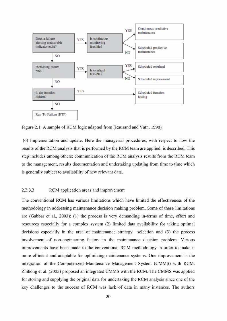
20

Figure 2.1: A sample of RCM logic adapted from (Rausand and Vatn, 1998)

(6) Implementation and update: Here the managerial procedures, with respect to how the

results of the RCM analysis that is performed by the RCM team are applied, is described. This

step includes among others; communication of the RCM analysis results from the RCM team

to the management, results documentation and undertaking updating from time to time which

is generally subject to availability of new relevant data.

2.3.3.3 RCM application areas and improvement

The conventional RCM has various limitations which have limited the effectiveness of the

methodology in addressing maintenance decision making problem. Some of these limitations

are (Gabbar et al., 2003): (1) the process is very demanding in-terms of time, effort and

resources especially for a complex system (2) limited data availability for taking optimal

decisions especially in the area of maintenance strategy selection and (3) the process

involvement of non-engineering factors in the maintenance decision problem. Various

improvements have been made to the conventional RCM methodology in order to make it

more efficient and adaptable for optimizing maintenance systems. One improvement is the

integration of the Computerized Maintenance Management System (CMMS) with RCM.

Zhihong et al. (2005) proposed an integrated CMMS with the RCM. The CMMS was applied

for storing and supplying the original data for undertaking the RCM analysis since one of the

key challenges to the success of RCM was lack of data in many instances. The authors

21

proposed it for application in a power system and other engineering related systems. Beni

(2014) presented an enhanced RCM technique by integrating CMMS with RCM which,

according to the author, has the ability to change the maintenance strategy for a system

dynamically in a manner based on changing the maintenance strategy selection decision

criteria data. The maintenance strategy decision criteria data are not constant because the

operating condition of the asset and other factors that affect the life cycle of the asset are not

themselves constant. The use of CMMS was for dynamically managing the maintenance

strategy selection decision criteria data which is then applied as input data into the RCM

maintenance strategy selection methodology. The methodology was proposed for application

in the National Iranian Gas Company and its subsidiaries. Gabbar et al. (2003) also proposed

an integration of CMMS and RCM such that the CMMS dynamically manages and updates

the RCM analysis data which is then fed dynamically into the RCM methodology to

subsequently change the maintenance strategies of the studied system. In order to ascertain

the applicability of the technique the authors applied it to a nuclear power plant water-feed

process.

Another improvement that was carried out on the conventional RCM technique was the

introduction of the idea of ‘soft’ and ‘hard’ life by Crocker and Kumar (2000a) in order to

optimize total system maintenance costs. The authors defined hard life as being the age at

which a component of a system or sub-system has to be replaced and on attaining that age the

system or sub-system housing the component is removed for subsequent salvage. They

defined ‘soft’ life as being the age a component of a system or sub-system will attain, after

which it will be rejected at the next opportunity the system or sub-system housing the

component will be recovered. From the study the hard life is the suitable replacement age for

safety-critical parts or components of an aircraft system while the soft life is ideal for

comparatively cheap components that may cause costly, unplanned rejections of an engine.

The author concluded that the new RCM approach can be utilized in order to select an optimal

maintenance strategy for military aero-engines. In another development Cheng et al. (2008)

proposed an integrated case based reasoning method combined with the RCM analysis

technique and referred to as IRCMA. IRCMA, in the authors’ opinion, is a better alternative

to the conventional Computer Aided Reliability Centered Maintenance (CARCMS) method

and it is already being used in place of the latter as the RCM analysis tool for China’s military

equipment.

22

The applications of RCM and the improvements carried out on the technique as discussed so

far, are in the fields of nuclear power, defense and the oil and gas sectors. However RCM and

improved RCM techniques have also been applied in the marine sector. Conachey and

Montgomery (2003) proposed an integrated spare parts holding model combined with the

conventional RCM technique for application in machinery equipment components of ship

systems. After performing the first three steps of the RCM analysis such as defining systems,

defining functions and functional failures and performing FMEA, the next step was to

categorise risk of failure modes. The authors suggested the use of a risk matrix and gave an

example of a risk matrix that classified failure modes into three risk categories; high risk,

medium risk and low risk. For the three categories of risk the following maintenance

strategies are applied as a means of mitigating the risk; for the high risk a one-time change or

redesign, for the medium risk undertaking condition monitoring or time based preventive

maintenance and for the low risk, run-to failure. The failure modes and corresponding

criticality ranking for each failure mode were then used to populate the RCM logic in order to

ascertain the exact maintenance strategy to be employed to detect from the onset or to

mitigate or eliminate failure. This was followed by determination of the maintenance task

interval and finally determination of spare parts holding. In a related paper Conachey (2005)

suggested the application of conventional RCM on the machinery system of a ship together

with an additional model to cater for the spare parts needs. The spare part model that was

incorporated into the conventional RCM was based on risk assessment. The author

recommended the basic tools such FMEA, RCM logic and a risk matrix generally applied for

the conventional RCM analysis, for implementation on the machinery equipment of the ship

system. It was concluded that the RCM technique is a relatively new maintenance

optimization approach in the maritime industry and that the industry players (owners and

operators) will fully embraced it due to the same benefits that other sectors have derived from

the implementation of the technique.

Lazakis (2011) presented an enhanced RCM technique based on a combination of the

managerial aspects of TPM and the technical aspects of RCM. This novel RCM approach is

referred to by the author as Reliability and Criticality Based Maintenance (RCBM). The

essence of the approach was to have an efficient maintenance system in place that will have

the results to improve reliability and downtime minimization of a ship system. In order to

achieve the aim of the study, the author applied reliability techniques and tools such as

Dynamic Fault Tree Analysis (DFTA), Failure Modes, Effects and Criticality Analysis

23

(FMECA) and fuzzy set theory in combination with TOPSIS in solving multi-criteria decision

problems. One such multi-criteria decision problem that was solved is the resolution of a

maintenance strategy selection problem which the author addressed with the Fuzzy-TOPSIS

methodology. The applicability of the author’s proposed enhanced RCM was demonstrated

with two case studies; a cruise ship diesel system and a Diving Support Vessel.

From the RCM discussion it can be seen that there are three key elements of maintenance that

the methodology is used to optimize; (1) risk assessment, (2) maintenance strategy selection

from different alternatives, and (3) maintenance task interval determination. A great deal of

work has been carried out with respect to improving the efficiency of RCM in optimizing

these three components and ensuring continuous asset reliability improvement, however there

remains scope for further improvement in all three aspects.

2.4 Risk assessment

The American Bureau of Shipping (2000) defined risk as the product of the probability of the

occurrence of a failure and consequence of the failure. Mathematically this is simply

expressed as:

Risk = failure probability x consequence of the failure (2.5)

While risk assessment, according to Cross and Ballesio (2003), is defined as being a

systematic method that combines diverse aspects of design and operation in assessing risk.

Arendt (1990) described risk assessment as activities involving hazard identification, chances

of the occurrence of failure estimation and the consequences of the failure estimation.

With the advent of risk-based inspection and maintenance in the 1990s in conjuction with

reliability maintenance, risk assessment has gained popularity in the maintenance world and it

is worth noting that risk assessment is clearly the most critical phase of risk-based

maintenance since maintenance decisions to be taken will be based on the assessed level of

risk (Arunraj and Maiti, 2007). Risk assessment is also a very important aspect of Reliability-

Centred Maintenance (RCM) though RCM is mainly intended for preserving the reliability of

plant equipment and systems. The risk assessment in the RCM process involves assessing the

risk of failure of equipment items and based on the assessed risk, an appropriate maintenance

24

strategy will be recommended. However the acceptable level of risk must be defined possibly

through a retrospective study of earlier successful items etc.

Some of the factors that affect the quality of the output from a risk analysis are; data sources,

human factors, methods and tools for performing the analysis itself, and the ability and

experience of the analyst.

2.4.1 Risk assessment approaches

In assessing the level of risk of an asset the risk analyst has the option of selecting from

among three different risk assessment approaches and, in general, the choice depends on the

availability of data for performing the analysis. The three different risk assessment approaches

are qualitative, semi-qualitative and quantitative (Khan et al., 2012).

2.4.1.1 Qualitative technique

In this approach risk is measured based on subjective judgement. As stated above, risk is the

product of the probability of failure occurring and the subsequent consequences of the failure

and these parameters should be determined using subjective judgement. In describing failure

consequences, terms such as minor, major, critical and catastrophic are utilised while the

probability of failure occurring is expressed using terms such as improbable, remote,

occasional, probable and frequent (American Bureau of Shipping, 2003). Since the means of

assessment are subjective, it follows that the mitigation measures chosen for risk reduction

will also be subjective. Qualitative risk assessments are generally applied when there is a lack

of quantitative data in terms of measurable quality and quantity. The techniques are usually

ideal for systems where risk is relatively small and well known from experience.

2.4.1.2 Quantitative technique

The use of this technique greatly depends on the availability of quantitative data (Carter et al.,

2003). As opposed to the subjective judgement used in the qualitative technique, judgement is

based on using probability analysis to determine numerical values for the probability of

failure occurrence and the consequences of failure (Khan et al., 2012). Some of the tools

available for quantitative risk analysis are; Fault Tree Analysis (FTA) and Event Tree

Analysis (ETA).

25

2.4.1.3 Semi-quantitative technique

In this approach the estimated numerical values necessary for the probability of failure

calculations and the corresponding consequences of failure are based on expert opinions using

available data from similar plants (Khan et al., 2012). With this assessment methodology,

scores are assigned, based on expert judgement, to each of the variables that affect the

probability of failure and the corresponding consequences and these are summed up in order

to give an estimate of the probability of failure and of its consequences (Khan et al., 2012).

This technique can supplement traditional tools such as FMEA, Hazard Operability Analysis

(HAZOP) and others tools used for quantitative techniques such as FTA and ETA

(Hauptmanns, 2004).

2.4.2 Risk assessment methods and tools

An analyst has the option of choosing from a variety of tools for performing risk analysis in

each of the three major phases of risk assessment; hazard identification, risk estimation and

risk evaluation. Some of the commonly used tools/methods will be discussed in the following

text with emphasis on the tools that will be subsequently used in this research. It should be

noted that one of the keys to successful risk assessment lies in the ability of the analyst to

choose the right method or combination of methods for a particular problem (American

Bureau of Shipping, 2000).

2.4.2.1 Checklist Analysis technique

A checklist is simply a list of questions about the plant system operation, maintenance, etc.

and the essence is to systematically check if functional need and requirements are fulfilled.

They are usually prepared based on the company’s experience, codes and standards employed

and are the simplest method for risk identification (Khan and Abbasi, 1998). The list indicates

items of conformance and non-conformance and for the non-conformance items carefully

prepared recommendations are made in terms of correcting whatever items are found to be

wrong or faulty. Khan and Abbasi (1998) identified some of the limitations of the checklist

approach which include:

(1) It takes a long time to develop a checklist and the result does not give full insight into

the system. The status of each analysis item are in the form of ‘Yes’ or ‘No’.

26

(2) The quality of the result is a function of the ability and the experience of the analyst

who compiled the checklist and interpreted the result.

(3) It cannot identify a hazard that has to do with system mis-operation such as leaks or

excessive heat generation nor can it tell the severity of operating conditions.

2.4.2.2 Hazard Operability Analysis (HAZOP)

HAZOP is a risk analysis and assessment tool that was developed by British Imperial

Chemical Engineering in the 1960s (Zhan et al., 2012). The basic principle of a HAZOP study

is that once there is a deviation from standard operating conditions of a system the result is a

potential hazard (Khan and Abbasi, 1998). Once a deviation has been identified (detected) the

next step is to find out the cause of the deviation and rank the corresponding level of risk in

the system. Lastly steps will be taken to mitigate the effect of the risk on the system (Zhao,

2008).

According to Khan and Abbasi (1998) HAZOP has some limitations. These include:

(1) Just like a checklist the quality of the result and actions will depend on the ability and

experience of the analysis team involved.

(2) The method assumes that the equipment has been built in accordance with appropriate

codes and standards; this is not always the case as there can be faulty designs and installations

as well.

Despite these limitations it is still one of the most common of tools that is used used for

hazard identification and risk assessment in the chemical processing industry, the

manufacturing industry and the power industry. In spite of its popularity in all of these sectors

only one application of HAZOP in the area of ship risk assessment has been reported in the

literature (Zhan et al., 2012).

2.4.2.3 Fault Tree Analysis

Geoff (1996) defined “fault tree as a method by which a particular undesired system failure

mode can be expressed in terms of component failure modes and operator actions. The system

failure mode to be considered is termed the top event and the fault tree is developed in

branches below this event showing its causes”.

The information that is fed into the fault tree will determine whether the approach is

quantitative or qualitative. Quantitative analysis is used if the occurrence or failure probability

27

of the top event is calculated based on the estimated or measured occurrence probability of

each basic event (Xing and Amari, 2008). The qualitative fault tree, on the other hand only

gives a description of the combination of the basic events causing the potential problem of

interest (American Bureau of Shipping, 2000). The qualitative techniques thus cannot

quantify or estimate the level of risk but could help in identifying potential hazards and their

significance (Halme and Aikala, 2012). The fault tree analysis technique is most suited for

analysing top events (system failures) resulting from relatively complex combinations of

component failures (American Bureau of Shipping, 2000).

Just like every other risk analysis tool it has some limitations according to (Khan et al., 2012)

which include:

(1) The assumption in the quantitative technique is that the likelihood of basic events is

precisely known which is not true because the data collection mode is characterised by a high

degree of uncertainty.

(2) The assumption that component failures or basic event failures are independent is

absolutely untrue in real life systems.

These two assumptions will translate to having an inaccurate risk level analysis assessment

thereby resulting in potentially wrong maintenance decisions for the particular failure mode

under consideration.

2.4.2.4 FMEA

Siddiqui and Ben-Daya (2009) defined Failure Mode and Effect Analysis (FMEA) “as a

systematic failure analysis technique that is used to identify the failure modes, their causes

and consequently their fallouts on the system function”. The development and application of

the FMEA methodology dates back to 1949 and the United States Army and in the 1970s its

was embraced by the automotive, aerospace and manufacturing industries (Scipioni et al.,

2002). Today FMEA is a commonly used risk assessment tool in the production of hardware

such as mechanical and electronic components (Scipioni et al., 2002). “The introduction of

FMEA to on–board ship operations can be considered as a step in a new direction” according

to Cicek and Celik (2013). When FMEA is combined with criticality analysis (CA) it is

referred to as Failure Mode Effect and Criticality Analysis (FMECA) and its essence is to

rank the impact of each of the failure modes for the various components that make up the

entire system (Headquarters Department of the Army, 2006, Sachdeva et al., 2009a).

According to Ben-Daya (2009) FMEA basically performs three functions. These are:

28

(1) To identify and recognize potential failures including their causes and effects.

(2) To evaluate and prioritize identified failure modes.

(3) To identify and suggest actions to either eliminate or reduce the chance of the

potential failures from occurring.

The technique can be applied to any well-defined system but it is best suited for the risk

assessment of mechanical and electrical systems (e.g. fire suppression systems, propulsion

systems) and the approach can either be quantitative or qualitative, (American Bureau of

Shipping, 2000, Headquarters Department of the Army, 2006). The availability or non-

availability of failure data will determine to a large extent the approach that is used in

carrying out FMEA risk assessment. A quantitative approach is used when variables such as

failure rate (λi), failure mode ratios (αi ), failure effect probability (βi ) and its operating time

(t) are known and are used to generate the criticality number (CN) which can then be used to

rank ith failure mode (Headquarters Department of the Army, 2006, Braglia, 2000). This can

be represented mathematically as:

CNi = αi x βi x λi x t (2.6)

In applying the qualitative method each failure mode is rated or ranked by developing a risk

priority number (RPN) which is computed by multiplying the severity rating (S) by both the

occurrence probability (O) and the detection rating (D):

RPN = S x O x D (2.7)

Qualitative terms are used to determine these three parameters, usually on a numerical scale

of 1 to 10 having been determined based on collective expert opinion (Sachdeva et al., 2009b,

Siddiqui and Ben-Daya, 2009, Ling et al., 2012, Kahrobaee and Asgarpoor, 2011, Zammori

and Gabbrielli, 2012, Braglia, 2000). Tables 2.1 to 2.3 show the qualitative scales that are

commonly used for occurrence ranking, severity ranking and detection ranking.

29

Table 2.1: Occurrence ranking, copied from (Headquarters Department of the Army, 2006)

30

Table 2.2: Severity ranking, copied from (Headquarters Department of the Army, 2006)

Table 2.3 Detection ranking, copied from (Headquarters Department of the Army, 2006)

31

FMEA is generally the preferred tool for reliability and risk assessment studies, probably

because it can easily be understood and applied (Braglia, 2000). Some other reasons why it is

frequently employed, according to Ben-Daya (2009), are that it can:

(1) Help to reduce the chances of a catastrophic failure that can result in injuries and/or

have an adverse effect on the environment.

(2) Optimize maintenance efforts by suggesting applicable and effective preventive

maintenance tasks for potential failure modes.

Despite the popularity of FMEA, it has serious flaws (Bowles, 2003). For example a

particular failure mode might have a high severity ranking, a high occurrence and a very low

detection ranking, because it can easily be detected and which may result in having a low

overall risk ranking i.e RPN (Ling et al., 2012). The result may be that the analyst

recommends preventive maintenance instead of predictive maintenance or requiring redesign

because of the misleading RPN. Some authors have suggested the removal of the detectability

element from the RPN calculation (Bowles, 2003, Fleming and Wallace, 1986, Bowles, 1998)

as a solution to this potential problem. Conversely some authors are of the opinion that the

three attributes are equally important and thus as such the detection attribute should not be

removed (Narayanagounder and Gurusami, 2009). Other limitations of FMEA are:

(1) The technique takes into account only three attributes in rating risk whereas there are

other important factors such as economic cost, production loss, environmental impact etc.

which are not taken into consideration (Braglia, 2000, Sachdeva et al., 2009b, Zammori and

Gabbrielli, 2012, Liu et al., 2011)

(2) Different combinations of three attributes can yield the same RPN number but the risk

level may be totally different (Sachdeva et al., 2009b, Kutlu and Ekmekçioǧlu, 2012, Liu et

al., 2012, Sharma and Sharma, 2012).

(3) It requires the services of very experienced and well trained teams (Teng and Ho,

1996).

(4) The RPN formula is questionable and debatable (Liu et al., 2012, Liu et al., 2011,

Kutlu and Ekmekçioǧlu, 2012, Geum et al., 2011, Chin et al., 2009b)

FMEA is, however a key component of the Reliability-Centered Maintenance methodology

and ABS specifically require the bottom-up FMEA approach when performing RCM analyses

(Conachey, 2005).

32

The traditional FMEA has some limitations just like every other risk assessment tool however

many alternative variations and methods have been advocated in the literature in order to

overcome or minimise some of these challenges. (Souza and Alvares, 2008) applied the

traditional FMEA in conjunction with Fault Tree Analysis (FTA) as a risk assessment tool for

the application of Reliability Centred Maintenance. The methodology was used to study and

analyse the failure mode of a hydraulic Kaplan turbine of a hydroelectric plant. The

comparative study showed that the two tools can complement each other for the execution of

an effective predictive maintenance plan on the basis that the FMEA analysis provided the

information required for the FTA basic event. However when the results of the risk analyses

of the FTA and the FMEA were compared some of the items that the FTA identified as being

critical were shown to be non-critical in the FMEA and vice versa. The discrepancy was

considerable and this could be attributed to the author using the results of only the probability

of failures of the basic event in the FTA in comparing the results of the FMEA instead of

using the probability of failures multiplied by the consequence of failures. Other

improvements in literature to the classical FMEA and limitations that prompted the need to

develop new tools for prioritising risk of failure modes are discussed in Chapters 3 and 4.

2.5 Maintenance strategy selection

One of the main challenges of maintenance management is the selection of the appropriate

maintenance strategy for each equipment item in the system because not all maintenance

strategies are applicable and cost effective for different components. Hence choosing the right

maintenance strategy for the system will help maintain a balance between the system

availability and cost of performing the maintenance. However when choosing the type of

maintenance strategy for a ship machinery system or other complex related ship systems,

several conflicting decision criteria must be taken into consideration such as cost, reliability,

availability and safety. These make maintenance strategy selection analysis critical and

complex and the investigation fundamental and justifiable (Bevilacqua and Braglia, 2000).

Despite the significance of the subject, only a few studies have dealt with maintainance

selection policy problem (Bertolini and Bevilacqua, 2006).

There are different maintenance strategies that can be used for mitigating the different failure

modes of a marine machinery system. Generally there are three types of maintenance strategy

that are available for maintenance practitioners to choose from. The three maintenance

33

strategies and a review of the methods utilised for the selection of the optimum strategy for

each of the different component/failure modes of the system are discussed next.

2.5.1 Maintenance strategies

According to Pintelon et al. (2006) a maintenance strategy is generally viewed from the

perspective of maintenance policies such as breakdown maintenance, preventive maintenance

and predictive maintenance and sometimes RCM or TPM. It is worth noting that the

maintenance strategy is one of the most influential factor affecting the effectiveness of a

maintenance system (Stanojevic et al., 2000, Stanojevic et al., 2004) and the process of

estimating the optimal combination of maintenance strategies for different plant system

equipment items is a very hard and complex task as the maintenance program must combine

both technical and management requirements (Sachdeva et al., 2009b, Bertolini and

Bevilacqua, 2006, Bevilacqua et al., 2000). The selections usually require a vast amount of

information relating to the following decision criteria (Bertolini and Bevilacqua, 2006):

manpower utilization, cost and budget constraints, safety factors, environment factors and

Mean Time Between Failure (MTBF) for each piece of equipment.

2.5.1.1 Run-to-Failure

The rationale of the run-to-failure management approach is simple and straightforward.

When a machinery equipment item fails it is fixed. That is to say equipment is allowed to fail

before any maintenance (repair or replacement) is carried out and, as such, resources are not

deployed until equipment breaks down. It is, in fact, a no-maintenance approach to

maintenance management of an asset and it is generally the least cost effective technique of

maintenance management, since the maintenance costs are higher and plant availability is

lower. In fact maintenance cost analysis revealed that repair carried out in reactive mode is

nearly three times higher in cost than that carried out in preventative mode (Mobley, 2001)

This type of maintenance is usually effective for non-critical and low cost components and

equipment in a system (Pride, 2008). For the plant manager to know that a component is non-

critical, criticality analysis is carried out and, based on the result, an appropriate maintenance

strategy is recommended for the plant equipment.

34

2.5.1.2 Preventive Maintenance

Preventive maintenance is defined as maintenance actions performed on plant systems at a

definite interval with the aim of preventing wear and functional degradation, extending the

useful life and mitigating the risk of catastrophic failure (Sullivan et al., 2004) and it concerns

itself with such activities as the replacement and renewal of components, inspections, testing

and checking of working parts during their operation (Ebrahimipour et al., 2015). In utilising

this approach for maintenance management, equipment repairs or replacement are performed

at pre-established intervals. The length of the intervals is usually based on equipment items’

industrial average-life such as Mean Time Between Failures (MTBF). However some plant

managers rely on machine or component manufacturer’s recommendation to schedule

preventive maintenance activities.

For the shipping industry, the IMO in 1993 set the foundations for preventive maintenance

implementation by releasing the International Safety Management (ISM) code (IMO 1993).

Chapter 10 of the ISM code clearly states the procedure and the duties of the shipping

industry for preventive maintenance implementation in such a way that international

regulations are adhered to strictly.

The major merit of PM is its ability to increase the average life of equipment items and to

reduce the risk of catastrophic failure (Sullivan et al., 2004). However despite the numerous

benefits of PM, the major limitation is that it often results in unnecessary repair or

replacement. Another limitation is the difficulty in evaluating the optimum interval of

performing the maintenance task as this may take years of data collection and analysis (Chen,

1997).

The time based preventive maintenance approach can further be divided into two categories as

follows:

(1) Scheduled overhaul: a maintenance approach where equipment overhaul or repair is

carried out on a specified interval basis. This policy is suited to equipment or machinery with

identifiable age when failure rate function rapidly increases and large elements of the

equipment or machine must survive to that age and also where reworking can restore the

machine to an acceptable operational condition (Rausand, 1998).

(2) Scheduled replacement: This refers to maintenance techniques in which equipment or

a unit of it is replaced on a scheduled basis. This is usually ideal when equipment or machines

35

are exposed to critical failure; large units of the equipment or machines must survive to at

least the replacement time and the failure type must be of major economic consequences

(Rausand, 1998).

2.5.1.3 Condition Based Maintenance

This refers to the maintenance approach in which the condition of an item or piece of

equipment is monitored in order to detect potential failure and recommend appropriate

corrective action. The CBM are generally of two types; the continuous on-condition task and

the scheduled on-condition task (Rausand and Vatn, 1998). The continuous on-condition task

which is referred to as online condition based maintenance (ONCBM) in Chapter 5 is the

approach where the condition of an equipment item is monitored uninterruptedly using

diagnostics devices. The major disadvantage of this type of approach is that it is expensive

(Jardine et al., 2006). The scheduled on-condition task is referred to as offline condition based

maintenance (OFCBM) in Chapter 5, is an inspection performed on an equipment item at

regular interval with the aim of detecting potential failure (Rausand and Vatn, 1998). The

check carried out on equipment items is performed by maintenance practitioners or operators

with or without the use of diagnostic tools. This approach is effective and yet more cost

effective than the continuous on-condition task and as such more attractive to most industries

and the maritime industry inclusive. However the major challenge of the scheduled on-

condition task is the problem of determining the appropriate interval for performing

inspection task (Jardine et al., 2006).

In designing a condition monitoring program for ship machinery systems, general procedures

to be followed had been put in place by BSI/ISO 17359 (2003). The standard includes

procedures for equipment auditing, criticality assessment and overview of the condition

monitoring procedure and the determination of the maintenance action to be used.

The technique for scheduling maintenance tasks is the major difference between time based

preventive maintenance and condition based maintenance. While the time based preventive

maintenance activity is scheduled based on average life evaluated using historical data of the

particular piece of equipment, the condition based maintenance activity is scheduled in

response to a performance degradation observed from diagnostic device readings and/or

36

human sensing which deviate from standard equipment operating conditions (Noemi and

William, 1994).

2.5.2 Maintenance strategy selection methods

The use of the Multi-Criteria Decision Making (MCDM) such as such as the Analytical

Hierarchy Process (AHP), the Analytical Network Process (ANP) and the Technique for

Order Preference by Similarity to an Ideal Solution (TOPSIS) in making optimum decision

for when faced with multi-criteria decision problem is becoming popular (Gandhare and

Akarte, 2012, Bevilacqua et al., 2000). One of such multi-criteria decision problem is the

maintenance strategy selection. These techniques have either been applied singly or integrated

with one another or they have been used in conjunction with other tools such as fuzzy set

theory and mathematical programming. (Bevilacqua and Braglia, 2000) applied AHP to select

the ideal maintenance strategy for an integrated gasification and combined cycle plant. The

analysis took into consideration five possible alternatives: preventive, predictive, condition-

based, corrective and opportunistic maintenance. The authors used AHP in conjunction with

Failure Mode Effect and Criticality Analysis (FMECA) principles in order to choose the ideal

maintenance strategy for each analysed item in the plant. Other examples of the application

of AHP for maintenance strategy selection are: Triantaphyllou et al. (1997) proposed an AHP

technique for the selection of a maintenance strategy taking into consideration four

maintenance decision criteria; Nyström and Söderholm (2010) presented a methodology

based on AHP for prioritising different maintenance actions in railway infrastructure, and

Labib et al. (1998) developed a model based on AHP for optimum maintenance decision

making for an integrated manufacturing system.

Bertolini and Bevilacqua (2006) presented an integrated AHP and Goal Programming (GP)

technique such that the best strategies for the maintenance of centrifugal pumps in an oil

refinery is chosen. The model that was proposed considered decision criteria such as account

budget and number of man-hour constraints in comparring three alternative maintenance

strategies (corrective, preventive and predictive). The authors concluded that the application

of an integrated AHP and GP methodology proved to be a viable tool for minimization of

maintenance cost (Bertolini and Bevilacqua, 2006). Similar to this approach, Arunraj and

Maiti (2010) used AHP and a GP method for the selection of a maintenance strategy for a

benzene extraction unit within a chemical plant. Equipment failure risk and the cost of

37

performing maintenance were considered as the relevant decision criteria. AHP was used to

assign weights to the decision criteria by means of pairwise comparison and the GP

considered the assigned weight to rank the alternative maintenance strategies (corrective, time

based, condition based and shutdown maintenance). The main improvement to the work of

Bertolini and Bevilacqua (2006) was the use of the Fussell-Vesely (F-V) importance measure

by the authors in order to estimate the risk contributions of different items of equipment. Zaim

et al. (2012) reported on the use of a combination of AHP and ANP techniques for selecting

the optimum maintenance strategy for a newspaper printing facility located in Turkey. From

the comparative study, the two techniques yielded almost the same results.

The use of integrated fuzzy logic and MCDM (such as AHP) for maintenance strategy

selection has also been reported in literature. Al-Najjar and Alsyouf (2003) used integrated

fuzzy logic and AHP techniques to select the most cost effective maintenance strategy for a

pump station. Wang et al. (2007) also proposed a fuzzy logic-AHP technique in order to select

optimal maintenance strategies for different equipment items in a manufacturing firm.

The Reliability Centered Maintenance (RCM) technique is also widely used (Bevilacqua and

Braglia, 2000, Mohan et al., 2004). “RCM represents a method for preserving functional

integrity and it is designed to minimise overall maintenance costs by balancing the higher cost

of corrective maintenance against the cost of preventive maintenance” (Crocker and Kumar,

2000b). RCM has been applied to a greater or lesser extent in the maritime industry for

example the use of RCM logic diagrams in order to select the most appropriate maintenance

strategy for different components of a system from the failure modes perspective (Conachey,

2005, American Bureau of Shipping, 2004). However the use of RCM is a very time

consuming exercise and generally limited to some specific equipment (Waeyenbergh and

Pintelon, 2004). Another limitation of the RCM technique in selecting maintenance strategies

is that it does not allow for ranking of maintenance alternatives such that the optimum

solution can easily be selected. This prompted Lazakis et al. (2012) to develop a maintenance

strategy selection methodology based on the integration of fuzzy set theory and TOPSIS for

the selection of the maintenance strategy for a diesel generator in a cruise ship. The

maintenance strategy selection model that the authors proposed compared three alternative

maintenance strategies (corrective, preventive and predictive maintenance) against eight

decision criteria: maintenance cost, efficiency/effectiveness, system reliability, management

commitment, crew training, company investment, spare parts inventories and operation loss.

38

From the analysis, condition based maintenance (CBM) was considered as the optimum

maintenance strategy for the cruise ship diesel generator. However some doubts remain with

regard to the practical use of the fuzzy approach because of the difficulty in testing and

developing extensive sets of fuzzy rules (Zammori and Gabbrielli, 2012, Braglia, 2000).

Additionally some important decision criteria such as applicability for maintenance strategy

selection especially when dealing with the problem from the system failure modes perspective

were not taken into account in Lazakis et al. (2012). In further work, Lazakis and Olcer

(2015) aimed to improve the performance of the fuzzy-TOPSIS methodology by integrating

AHP into it. AHP was introduced to assist in the weighting of the decision criteria. The result

of the enhanced technique yielded preventive maintenance as the optimum maintenance

strategy for the for ship diesel generator.

Goossens and Basten (2015) utilized AHP in the selection of maintenance strategies for naval

ship systems. The authors involved three different groups within the industry in the decision

making process namely: the shipbuilders, the owners/operators and the Original Equipment

Manufacturers (OEM). In selecting the optimal maintenance strategy for the ship system from

three maintenance strategies; corrective, time/use-based maintenance and condition based

maintenance, three level decision criteria were applied. The first level consisted of two

decision criteria; the second level consisted of eight and the third level consisted of 29. From

the analysed results, the maintenance strategy preferred by the shipbuilder, owner/operator

and the OEM is condition based maintenance. However the structuring of the problem made it

computationally intensive as it required formation and analysis of numerous pairwise

judgements from experts.

Resobowo et al. (2014) also applied AHP in prioritizing the factors that affect military ship

maintenance management. In this case, the factors considered were; cost, availability,

reliability, safety, human resource, operations, types of ship and ship characteristics. These

factors were ranked using planned maintenance, preventive maintenance and routine

maintenance as decision criteria. According to the authors the result of the analysis revealed

that the most important factor is human resource. The major interest of the authors was to

identify important factors for making maintenance decisions and as such does not completely

address the problem of maintenance strategy selection.

39

It is obvious that there is a need for a more systematic approach that can easily incorporate

qualitatively and/or quantitatively the maintenance alternatives selection criteria for marine

system applications. On this basis one of the objectives of this research was to develop an

alternative maintenance strategy selection method which avoids the limitations of the

approaches used in literature.

2.6 Maintenance interval determination

After determining the type of maintenance task for each of the failure mode/components of an

asset or machinery item, the next task is to determine the interval for carrying out the

maintenance tasks. This process is an essential phase of the different maintenance

optimization techniques (RBM, TPM and RCM). In this research the maintenance tasks that

are considered for preventing or mitigating the effects of failure are; CM or RTF, scheduled

overhaul, scheduled replacement, offline condition based maintenance (physical inspection)

and online condition based maintenance (use of diagnostic tools). For all of these various

maintenance types, different models have been developed by researchers for determining the

intervals for performing them and they have been applied in different fields with variations to

suit specific industrial needs. However the basic principle for the determination of the interval

is to have a balance between the cost of achieving the highest reliability and the cost of

unexpected failure. In the following Sections the different models that have been developed

by different researchers for determining intervals for (1) scheduled replacement and (2)

offline condition based maintenance (inspection) are discussed.

2.6.1 Scheduled replacement interval determination

As previously stated, preventive maintenance involves repair or replacement activities being

performed at regular intervals. Hence scheduled replacement is one of the techniques that is

used in preventive maintenance in order to recover the functions of an equipment item.

Bahrami-G et al. (2000) defined it as a practice that entails decision making, based on certain

criteria regarding the optimal time to replace an equipment item so as to reduce or eliminate a

sudden breakdown. Optimization techniques are used to define the appropriate intervals for

the replacement of the equipment item in order to have a balance between availability of the

40

equipment items and the cost of the related maintenance. Generally two conditions must be

satisfied to justify the use of scheduled replacement as a strategy in maintaining equipment.

These are: (1) the value of Weibull shape parameter β of the equipment/components statistical

variability must be greater than 1 and (2) the cost of the replacement activity as a result of

failure must be greater than the cost of planned replacement. It therefore means that data on

the failure parameters of the equipment and related cost information are essential in order to

ascertain whether or not there is the need for a scheduled replacement to be carried out. This

information is also required as an input into the replacement model in order to determine the

optimum interval for replacement. Once it is ascertained that scheduled replacement is the

optimum option for performing the recovery or sustainment of items of equipment, the most

appropriate interval is then to be determined. From the literature two popular models have

been generally applied and these are; the Age Replacement Model (ARM) and the Block

Replacement Model (BRM) (Aven and Jensen, 1999).

For the ARM, an equipment item is replaced with respect to a predetermined age (tp) or at

failure. In this respect if failure occurs before the predetermine interval time, replacement is

carried out at failure otherwise replacement is at the predetermined age. Furthermore if an

equipment item is replaced due to failure, the replacement equipment is assumed to be as

good as new and as such the maintenance practitioner would have to wait for another tp to

elapse before carrying out the next replacement. The universal ARM mathematical model,

which is generally used for determining the appropriate time interval (tp) for scheduled

replacement is the one that was proposed by Barlow and Hunter (1960) and it is represented

as follows:

𝐶(𝑡𝑝) =𝐶𝑎 (1 − 𝑅(𝑡𝑝)) + 𝐶𝑏𝑅(𝑡𝑝)

∫ 𝑡𝑓(𝑡)𝑑𝑡𝑡𝑝0

(2.8)

Where:

𝐶(𝑡𝑝) is the cost function per unit time

𝐶𝑎 is the cost of unit failure replacement

𝐶𝑏 is the cost of unit scheduled replacement

𝑡𝑝 is the given scheduled replacement interval and

𝑓(𝑡) is the probability density function

𝑅(𝑡𝑝) is the Reliability function

41

The essence of this age replacement model is to evaluate cost of equipment replacement for

different values of ‘𝑡𝑝’. The value of 𝑡𝑝with the lowest cost is then chosen as the optimum

replacement interval. Hence the main purpose of this model is to minimise the cost of

replacement of equipment.

For the block replacement model, however equipment/components are replaced at constant

time intervals and in the case of failure before the constant time interval has elapsed the

equipment/components are replaced and will be replaced again once the same constant time

interval has passed. This type of replacement model can then result in unnecessary

replacement of equipment/components. Hence the generally accepted perception that the

ARM is more cost effective than the BRM. Nevertheless the BRM can be applied for less

expensive equipment items whose replacement can be carried out in a group. The only

advantage of the BRM over the ARM is that BRM is easier to apply and manage since

replacement is performed at regular intervals as opposed to ARM where the maintenance

practitioner would have to consider the time for replacement at failure before knowing the

exact date that the next preventative replacement will be performed. The general BRM

mathematical model is the one developed by Barlow and Hunter (1960) represented as

follows (Ahmad and Kamaruddin, 2012):

𝐶(𝑡𝑝) =𝐶𝑏 + 𝐶𝑎 . 𝑁(𝑡𝑝)

𝑡𝑝 (2.9)

Where 𝑁(𝑡𝑝) is the number of failures expected in an interval of 0 to 𝑡𝑝. As in the case of

ARM, the main purpose of this model is to obtain an optimum replacement interval at the

least cost.

These models (ARM and BRM) and variations have been applied in solving replacement

problems for both single unit and multi-unit systems in different industries. Since in this

research ARM has been chosen as the scheduled replacement model, discussion with respect

to review of existing work in the literature in terms of application and advancement will focus

on it.

2.6.1.1 ARM and BRM applications and improvement

Huang et al. (1995) developed a standard solution for the ARM that was proposed by Barlow

and Hunter (1960) and for ease of use it was organised in the form of tables and charts.

42

Another important feature of the solution, in addition to organising it in tables, is in the

reduction of input parameters by using a cost ratio (ratio of 𝐶𝑎 to 𝐶𝑏) in place of the actual

cost of failure replacement (𝐶𝑎 ) and cost of preventive replacement (𝐶𝑏). The algorithm

developed for the standard solution technique was applied to various hypothetical examples in

order to demonstrate the applicability of the technique. In their paper Cheng and Tsao (2010)

applied the standard solution for the determination of the preventive replacement

maintenance interval for a rolling stock component. Das and Acharya (2004) presented two

age-based replacement models for preventative replacement of an equipment item. The two

preventive replacement policies included consideration of the equipment failure delay time

(the time between the point of equipment failure initiation and the point at which the

equipment eventually failed). In the first model, the trend of the degradation of the equipment

during the delay time was utilised in order to determine the preventive replacement interval.

Hence, for this policy, replacement due to failure or prevention of failure is performed after a

fixed period during its delay time. The second policy, according to the authors, is an

opportunistic age replacement technique where a failing equipment item or component is

replaced at the next available maintenance opportunity. Finally the authors opined that the

two policies although designed for a single unit system were capable of addressing a multi-

unit system when there is a difficulty in tracking the whole life of each individual equipment

item or component. Jiang et al. (2006) investigated the relationship between the preventive

effect produced from alternative replacement intervals and corresponding cost savings. The

preventive replacement models that they studied were the age and the block preventive

replacement models. From the results reasonable cost savings can be derived if the system is

replaced when it has reached satisfactory age. The authors also opined that the often

increasing failure rate of the equipment or components does not necessarily translate to

representing ‘satisfactory age’ and this has to be determined by the maintenance practitioners

based on the maintenance goal.

Ahmad et al. (2011a) utilised the age based model that was developed by Hunter and Barlow

in revising the preventive replacement interval for a production machine in the processing

industry. The important feature of their approach was the consideration of the covariate effect

on the life of the machine. In the real sense the actual state of the machine was considered in

the determination of the preventive replacement interval of the machine. The authors

compared the revised replacement interval (inclusion of the covariate effect) with the

replacement interval (without covariate effect). From the result, the revised preventive

43

replacement interval and the replacement interval without the covariate effect differed

considerably. While the revised produced a 21 day interval for replacement of the production

machine, the replacement interval without the covariate effect produced a 35 day interval for

the replacement of the production machine. Bahrami-G et al. (2000) presented a new model

for the preventive replacement of an equipment item or component that is experiencing an

increasing failure rate. The model proposed is a simplified version of the BRM that was

developed by Hunter and Barlow. A case study of an equipment item whose failure rate

followed a normal distribution was applied to determine the benefits and suitability of the

technique. According to the authors, the results obtained from the model almost perfectly

matched the result from that of Hunter and Barlow whose approach is more computationally

challenging. They concluded that the proposed model will aid the maintenance practitioner to

make more cost-effective decisions.

2.6.1.2 MCDM tools application for scheduled replacement interval determination

based on ARM and BRM

The essence of undertaking preventive maintenance is to reduce the chances of failure of plant

equipment such that plant reliability and availability is optimised. The reliability of a system

is dependent on the reliability of the individual components/equipment items that collectively

make up the system and in order to achieve this aim, a suitable preventive maintenance and

inspection programme should be in place (Duarte et al., 2006)

One of the greatest challenges of the preventive maintenance approach is in the selection of

the optimum interval to perform preventative maintenance tasks on equipment items (Duarte

et al., 2006). This is because, if the intervals are not properly timed, it can result in over-

maintenance and a waste of resources and man-hours due to premature replacement or repair

of equipment items or an even worse case scenario, in that under-maintenance can result in

catastrophic failure and invariably production loss and the company’s image being damaged.

This makes the subject of interval selection for a preventive maintenance task an important

issue worthy of thorough investigation. There are quite a number of articles published in the

literature which are based on a single criterion for making decisions for preventive task

interval selection (Almeida, 2012, Gopalaswamy et al., 1993) and yet a number of them are

too abstract often requiring a high level of mathematical and statistical skills thereby limiting

the practicability of their use in real life situations (Vatn et al., 1996, Duarte et al., 2006,

Huang et al., 1995). In addition, the application of these single criterion based methodologies

44

is neither reliable nor flexible for effective decision making with respect to interval selection

(Gopalaswamy et al., 1993).

However there are some limited studies that deal with the use of the MCDM approach to

selecting intervals for preventive maintenance tasks (Gopalaswamy et al., 1993, Chareonsuk

et al., 1997) but they were applied for land based systems with no applications reported for

maritime systems. Cavalcante and De Almeida (2007) presented a preventive maintenance

decision model based on a combination of PROMETHEE II and Bayesian technique

considering two decision criteria; cost and reliability. In a similar work (Cavalcante et al.,

2010) also proposed an integrated PROMETHEE based methodology combined with

Bayesian technique and, in addition, accounting for possible uncertainty in maintenance data.

Chareonsuk et al. (1997) also proposed a PROMETHEE multi-criteria decision making

methodology for the selection of preventive maintenance intervals. The authors applied the

Huang et al. (1995) assumption that corrective replacement cost and preventive replacement

cost can be in the form of a ratio in the case of a situation with a lack of data. The cost ratio

was then varied for different assigned alternative replacement maintenance intervals in the

expected cost replacement model in order to obtain corresponding values of cost and

reliability factors. Finally PROMETHEE was applied in ranking alternative preventive

maintenance intervals with respect to the evaluated decision criteria, namely cost per unit and

reliability. The authors chose the replacement maintenance interval with the best

PROMETHEE index. The PROMETHEE technique used by these authors, has the challenge

of problem structuring thereby making the evaluation procedure complicated when more than

seven decision criteria are used. This approach will limit maintenance practitioners’ choice of

decision criteria for selecting optimum preventive maintenance intervals. Additionally the

authors’ approach for weighting decision criteria lacked flexibility as it only depends on

subjective rules without balancing it with an objective technique or using a compromise

between them.

From this literature review it is obvious that marine industries will benefit from the

application of MCDM techniques as tools for determination of optimum scheduled

replacement intervals. However a more systematic MCDM approach will be used in this

research that will avoid the limitations of the approach applied in the land base systems.

45

2.6.2 Inspection interval determination

In the condition based maintenance methodology there are basically two approaches for

monitoring the condition of an item of equipment or component; continuous and periodic.

These two approaches are also referred to as on-line condition based maintenance and offline

condition based maintenance in this research and are considered in detail in chapter 5. For the

continuous monitoring type, the condition of equipment is continuously monitored using

some form of measurement and/or diagnostic tools. The challenge of this approach is that it is

quite expensive and on this basis many maintenance practitioners prefer the periodic

monitoring technique which is more cost effective. However the major difficulty in the

periodic monitoring approach is in the timing of the inspection interval of the condition

monitoring activity because of the possibility of failures occurring between consecutive

inspections (Jardine et al., 2006). In the course of monitoring the state of an item, if a defect is

found, a repair or replacement task is scheduled and if possible it is executed immediately in

order to prevent the equipment from further deterioration. If inspections are not carried out

then slowly developing defects will go unnoticed and this can lead to catastrophic system

failure with severe economic loss for the company. However even if inspection tasks are

performed, if they are not properly timed then defects can still occur between successive

intervals. It is thus obvious that the determination of the optimal inspection interval is central

to the effective operational monitoring of any mechanical system. In conventional practice,

the inspection interval is determined by maintenance practitioners relying merely on

experience and/ or on the equipment manufacturers’ recommendation and the results from this

approach are far from optimal and are also conservative (Christer et al, 1997).

Inspection tasks as an alternative maintenance approach for an equipment item can only be

beneficial if there is a sufficient period between the time that a potential defect is observed

and the actual time of failure of the equipment. Hence the time that elapses between point of

failure initiation and the point when the failure becomes obvious is vital in estimating the

inspection interval. The time that elapse between point P and F is referred to the P-F interval

(TPF) within the RCM frame work and is illustrated in Figure 2.2.

46

Figure 2.2: P-F interval (Rausand, 1998)

In RCM, the P-F interval principle is applied in determining the frequency of the condition

monitoring of equipment and it was suggested that an inspection interval (T) be set at T ≤

TPF/2 (Arthur, 2005). The author however stated that one major challenge of the use of P-F

approach is that there are usually no data to evaluate P-F interval (TPF) and in most cases the

evaluation based on experts opinion. Moubray (1991), on the other hand, suggested five ways

of determining the inspection interval based on P-F but the author concluded that: “it is either

impossible, impractical or too expensive to try to determine P-F intervals on an empirical

basis”.

Apart from this approach that is used in the conventional RCM, other approaches have been

described in the literature for determining inspection intervals. In the majority of the

techniques cost optimization is the main decision criterion for determining the inspection

interval. Christer et al. (1997) proposed the Delay Time model and this concept has been

subsequently applied by many researchers either in its original form or as a variant in the

modelling of the problem of inspection intervals. This approach has surpassed alternative

models developed by other researchers for enhancing inspection intervals under different

situations (Wang et al., 2010). The DTM and its application in the modelling of inspection

programmes is discussed next.

47

2.6.2.1 Inspection interval determination based on delay time

The delay time concept has been employed by many authors in the field of maintenance

engineering in the modelling of inspection intervals (Scarf, 1997). The introduction of this

concept can be traced to Christer (1982). The delay time categorises the failure process of

machinery into two phases; the first phase is the time period from when the machinery is new

to the time that it starts showing signs of some degradation. The second phase is the time

period from when it starts showing some sign of performance degradation to the time when

the machinery eventually fails. The elapsed time between when the machinery first shows

signs of performance degradation and when it eventually fails is referred to as the delay time.

The Delay Time concept is in agreement with the P-F interval principle described within the

framework of the classical RCM. However the major difference is that each concept uses a

different technique in the evaluation of the time that elapses between the point of failure

initiation and the point failure eventually occur. For the delay time concept as proposed by

Christer, statistical distribution, such as a Weibull or an exponential distribution is utilised,

while the subjective technique is applied in determining P-F interval within the framework of

the classical RCM. Additionally in the delay time concept approach a different mathematical

modelling technique are used in the determination of the optimal inspection interval. The

delay time concept is illustrated in figure 2.3.

Figure 2.3: The Delay Time concept

In Figure 2.3, hf represents the delay time; pf represents the time of the initial machinery

performance sign of degradation and, f, represents the time that the machinery eventually

failed. The most appropriate time to perform a maintenance inspection is within the

machinery delay time and if it is performed then the fault will be detected and if the necessary

preventive maintenance such as repair or replacement of the machinery is executed, failure

48

will be averted. However if inspection is not carried out then, the machinery degradation will

continue until failure occurs at point f.

The delay time concept had been applied by several researchers in solving inspection

problems either for a single-unit system with a single failure mode or a multi-unit system with

multiple failure modes. The majority of researchers have focussed on the multi-unit system

with multiple failure modes. As stated earlier the concept of delay time was first introduced

by Christer (1982). In the paper the author applied the delay time concept in the development

of a cost model for building inspection maintenance. The model was utilised in determining

an appropriate inspection maintenance plan for a complex building as an alternative

maintenance strategy to the reactive approach. The following assumptions were made; (1) the

cost function varied within the delay time period and (2) inspection is perfect. In determining

the probability density function of the delay time a subjective method was proposed. On that

basis the author suggested that information such as time of failure initiation and delay time of

system parts should be obtained based on experts’ (that is engineers and inspectors) estimates.

A questionnaire developed for obtaining information from experts asked questions such as:

(1) For how long has it been since the fault was first observed (=HLA)?

(2) If repair or replacement is not performed, what duration of time could the fault stay

before parts may or will eventually fail (=HML)?

The delay time is then evaluated for each fault by hf = HLA+HML. The distribution for f(hf) is

therefore then obtained by observing a sufficient number of faults or defects.

Christer and Waller (1984a) applied the delay time concept in the development of two

inspection maintenance models for determining the inspection frequency for a complex

industrial system. Two different models; cost function and downtime function, were

constructed with the assumption that inspection is perfect. The cost function model shows the

relationship between the inspection interval, tp, and the cost for performing inspection at that

particular tp while the downtime function model shows the relationship between tp and the

resulting downtime for performing an inspection at that particular tp. The study was further

extended by introducing a model to cater for imperfect inspection. To demonstrate the

applicability of these methodologies some numerical examples were provided.

49

Christer and Waller (1984b) proposed both an integrated delay time model and a snapshot

model for determining an appropriate inspection plan for a canning-line plant in a production

company in order to reduce the potential system downtime. The integrated model was used to

model the downtime consequences of the system for every inspection maintenance interval.

The data applied in analysing the models was obtained subjectively i.e. based on experts’

estimates through the administering of questionnaires.

Wang (1997) proposed a novel model for estimating delay time distribution from a

combination of experts’ judgements in the face of insufficient or a lack of reliability data.

The author also proposed a technique for combining experts’ opinions as well as a model for

updating the estimate of delay time distribution in a situation where maintenance and

reliability data becomes available. One of the most important features of the approach is the

suggestion of the use of probability estimates rather than point estimates in designing a

questionnaire. The author compared the delay time distribution obtained using point estimates

with that obtained using probability estimates using two case studies. From the results of the

two case studies it was concluded that the delay time distribution obtained using a probability

estimate presented a better result than the one obtained using a point estimate. In a related

paper, Wang and Jia (2007) presented an integrated empirical Bayesian based technique with

a delay time model for determining the inspection interval for an industrial boiler. The

empirical Bayesian model was introduced for the purpose of utilising both subjective and

objective data in estimating delay time distribution parameters.

Tang et al. (2014) postulated that for a part of a system subjected to wear, objective data

should be applied in estimating parameters of the delay time model. On this basis they stated

that there is a need for continual functional inspection and repair for such systems so as to

reduce unscheduled downtime and lead to an increased record of maintenance data. Taking

into consideration the wearing parts of a system, a model based on the delay time concept was

developed for both perfect and imperfect inspections. To demonstrate the applicability of their

proposed models two case studies were presented; a blowout preventer core and a filter

element, both components of an oil and gas drilling system. Failure and maintenance data

obtained relevant to both parts were used to estimate the delay time distribution parameters.

The papers reviewed were studies that had been carried out in the non-maritime sector, such

as manufacturing, building and automobile industries. From the literature some limited work

50

has also been investigated by researchers with respect to application of the delay time concept

for developing inspection plans for maritime systems. Pillay et al. (2001) applied the expected

downtime model based on the delay time concept in order to determine appropriate inspection

periods or intervals for a fishing vessel equipment items. The inspection plan was developed

with the aim to reduce vessel downtime as a result of machinery failure that could occur

between discharge ports. To demonstrate the applicability of their approach, reliability data

gathered from the winch system and complemented with experts’ opinions, was applied to the

proposed model. The case study results showed that an inspection period of 12 hours was

appropriate for the system. In a related paper, Pillay et al. (2004) utilised both the expected

downtime function model and the expected cost function model based on the delay time

concept, in determining the optimum inspection period for the fishing vessel. In order to

obtain a compromise inspection period, the expected cost was plotted against expected

downtime consequences. Arthur (2005) used the delay time model in order to establish an

inspection interval for condition monitoring of an offshore oil and gas water injection

pumping system. The purpose of introducing the delay time concept was to produce an

alternative inspection plan for the system that was more cost-effective than the current

inspection regime of a one month cycle. Data was obtained from the Computerised

Maintenance Management System (CMMS) and subjected to screening. From the data

scrutiny, only one failure mode (bearing failure) was dominant for both the gearbox and the

motor while three failure modes (bearing failure, shaft failure and impeller failure) were

dominant for the pumps of the system. The author validated the observed data by comparing

it with published industrial reliability data. The validated data was then used as an input into

the delay time model in order to obtain the mean delay time and inspection interval for each

of the components of the system. The delay time model that was proposed produced an

inspection interval of 5 months against the current interval of 1 month with annual cost

savings of £21,000.

The approaches reviewed so far for maritime application suggested mainly single criteria

being utilised in the determination of inspection interval, however in practical situations

multi-criteria are generally involved in making such vital decision. These multiple criteria are

in most cases conflicting with one another and in such scenario, the use of Multi-criteria

decision making tools for aggregating decision criteria into a single analytical problem

becomes imperative.

51

2.7 Summary

In this chapter a thorough literature survey was conducted with respect to providing relevant

information pertaining to the development of multi-criteria decision making tools for

maintenance of marine machinery systems. The chapter introduced maintenance practitioners’

definition of maintenance, the negative implication of poor maintenance systems, types of

maintenance strategies and major elements of a maintenance system that must be optimised

and methods available for their optimisation. Three maintenance methodologies (RBM, TPM

and RCM) were discussed. Since the major focus in this study is RCM, it was discussed in

more detail in terms of analysis steps, application and improvements carried out by previous

researchers. It was observed that different tools are being used in optimising the different

elements of maintenance system within the framework of RCM. The three elements of

maintenance; risk assessment, maintenance strategy selection and maintenance interval

determination were discussed in detail and for the risk assessment with a particular focus on

FMEA. For the maintenance strategy selection, the three types of maintenance strategies;

corrective maintenance, preventive maintenance and condition based maintenance were

presented. A survey of methods used by previous researchers for the selection of the

appropriate maintenance techniques was considered. For the maintenance interval

determination the discussion was centered on scheduled replacement and scheduled

inspection type of maintenance with respect to current approaches, limitations of these

approaches and the need for multi-criteria decision making methods for application for marine

systems. From the review it was obvious that the tools utilised within the framework of RCM

for the optimisation of the three main elements of maintenance systems have limitations and

there was a need to develop alternative approaches that avoid such limitations. On this basis

alternative techniques have been developed and reported in Chapters 3 to 7.

52

Chapter 3 Risk Assessment using enhanced FMEA

3.1 Introduction

One of the key elements of a maintenance system is the assessment of risk of each equipment

item/component of the system such that the most important equipment items/components in

terms of risk criticality are given high priority in allocation of scarce resource. Risk

assessment is usually performed prior to the selection of the optimal maintenance strategy that

will mitigate the effect of failure since the optimal strategy to be selected is based on the

assessed risk. One of the most popular tools used for risk assessment of marine machinery

systems is Failure Mode and Effect Analysis (FMEA). With this analysis tool, risk is

represented in the form of a Risk Priority Number (RPN) which is computed by multiplying

the severity rating (S) by the occurrence probability (O) and the detection rating (D) for all

failure modes of the system. As previously stated in the literature review, the conventional

FMEA has been criticised as having several limitations such as inability to aggregate

imprecise ratings of multiple experts and inability to incorporate more than three risk criteria

(Su et al., 2012, Braglia, 2000). These challenges have been addressed in this chapter by

developing two novel methodologies for prioritising the risk of failure modes of marine

machinery systems. The first methodology integrates an averaging technique with RPN of the

conventional FMEA. This approach eliminates one challenge of the classical FMEA which is

the inability to aggregate imprecise ratings from experts. Other challenges of the classical

FMEA such as the inability to incorporate more than three decision criteria cannot be

addressed with this method. Hence a second approach is proposed for maintenance

practitioners who need to include other decision criteria such as economic factors or company

reputation in the decision making process. The second method integrates an averaging

technique with TOPSIS. While the averaging technique is applied as a means of aggregating

imprecise risk criteria ratings from multiple experts, RPN and TOPSIS are used in the ranking

of the risk of failure modes. The applicability and suitability of these methodologies for risk

prioritisation is demonstrated using two case studies.

The chapter is organised as follows: in Section 3.2 FMEA relevance in the marine industry is

discussed. In Section 3.3 the proposed risk prioritisation methodology is described. Section

53

3.4 presents the two case studies to demonstrate the applicability and suitability of the

proposed methodologies. Finally conclusions are presented in Section 3.5.

3.2 FMEA relevance in the marine industry background study and state of art

review

Marine machinery systems, no matter how well designed will not remain safe and reliable if

not properly maintained (Cicek et al., 2010a) . How to maintain such complex systems is still

a challenge in the maritime industry. One of the major problems is the selection of the

appropriate maintenance strategy for each piece of equipment/component of the system.

Different key players in the maritime industry have adopted various methodologies in

overcoming these challenges. One of the most popular methodologies adopted is Reliability

Centred Maintenance (RCM). RCM represents a method for preserving functional integrity

and is designed to minimise maintenance costs by balancing the higher cost of corrective

maintenance against the cost of preventive maintenance (Crocker and Kumar, 2000b) and it

uses decision logic diagrams in selecting maintenance strategies (Conachey, 2004, Aleksić

and Stanojević, 2007).

However in deciding on the appropriate maintenance strategy, a thorough risk analysis must

be carried out because the maintenance decision depends on the assessed risk. Different

techniques such as FMEA, Hazard and Operability Analysis (HAZOP) and checklist analysis

are available for risk analysis and within the marine industry, the American Bureau of

Shipping (ABS) requires FMEA to be employed in prioritising risk of failure modes within an

RCM framework (Conachey, 2005, Conachey, 2004, Conachey and Montgomery, 2003).

FMEA is a risk analysis tool which is used to define, identify, and eliminate known and/or

potential failures from the system, design, process, and/or service (Stamatis, 2003). It is one

of the most powerful tools for performing risk analysis for marine machinery systems with

values assigned to O, S and D by a team of experts using an ordinal scale, an example of

which is shown in Table 3.1. The ordinal scales in Table 3.1 were originally generated by

Ford Motor Company (Ford Motor Company, 1998) and have since been used by many

authors in assigning values to risk criteria in the prioritisation of failure modes of different

systems such as; marine diesel engine subsystems specifically the fuel oil system and

crankcase (Cicek and Celik, 2013, Cicek et al., 2010a), aircraft turbine rotor blades (Yang et

al., 2011), diesel engine turbocharger (Xu et al., 2002) and the cooling sub-system in an off-

54

shore plant (Sankar and Prabhu, 2000). The FMEA analysis usually involves a series of steps

which are presented in Figure 3.1.

As mentioned previously, the classical FMEA employed by the marine industry has been

criticised as having some flaws which limit the effectiveness of the tool in prioritising risk of

failure modes. Some of the flaws identified in the literature are (1) the inability of the

technique to take into account more than three attributes in prioritising risk thereby excluding

other important factors such as economic cost, production loss and environmental impact (Liu

et al., 2011), (2) the different combinations of the three decision criteria (detection, severity

and occurrence) yielding the same RPN value whereas the perceived risk might be totally

different (Kutlu and Ekmekçioǧlu, 2012) and (3) assumption that decision criteria are of equal

importance. These make the classical FMEA that uses RPN in prioritising risk unsuitable

especially in the marine environment and as such a more appropriate technique is needed for

the marine world.

The problem of aggregating diverse experts’ information which may be imprecise and

uncertain has been investigated by a few authors in recent years. Chin et al. (2009b) proposed

an FMEA system/methodology which uses a data envelopment analysis (DEA) technique for

capturing imprecise criteria ratings obtained from multiple experts. The decision maker has to

be familiar with linear programming concepts and software in order to apply this approach for

risk prioritisation. Yang et al. (2011) proposed an FMEA method which uses modified

Dempster-Shafer evidence theory (D-S) to aggregate the different opinions of experts for risk

prioritisation of the failure modes of rotor blades of an aircraft turbine. With this approach the

authors constructed a Basic Belief Assignment (BBAs) for all failure modes with respect to

risk criteria ratings from multiple experts. The BBAs of failure modes from different experts

are then aggregated with a Dempster-Shafer combination model. However the Yang

methodology is limited to aggregating the same complete distribution criteria rating from

different experts. This situation is not practically possible. Su et al. (2012) modified the BBAs

constructed by Yang in order to deal with a situation when different integer values of risk

criteria are assigned by experts. The Su methodology is also limited to complete distribution

criteria rating and although it is an improved version of the Yang methodology it can only

deal with a situation when integer values assigned by different multiple experts differ

marginally, otherwise the combination of multiple expert criteria ratings will be zero.

Additionally the aggregation techniques are computationally intensive and challenging.

55

In this chapter some of the drawbacks in the conventional FMEA technique are addressed

using two approaches for risk prioritisation: an AVeraging technique integrated with

conventional Risk Priority Number (AVRPN), and an AVeraging technique integrated with

TOPSIS (AVTOPSIS). The AVRPN technique is capable of aggregating precise, complete

distribution data and imprecise distribution data of multiple experts’ risk criteria ratings

through a novel approach using averages that can easily be understood and executed by

decision makers without resorting to specialised software or having the need to be familiar

with any programming concepts. The result obtained from the AVRPN method when applied

to a complete distribution risk criteria problem, closely matches the one generated from the

Yang et al. (2011) and Su et al. (2012) modified Dempster-Shafer evidence theory method.

AVTOPSIS also utilizes averages in aggregating imprecise data and, in addition to this, the

technique is capable of incorporating as many risk criteria as the decision maker would want a

decision to be based on.

56

Table 3.1: Ratings for occurrence (O), severity (S) and Detectability (D) in a marine engine

system, adapted from (Yang et al., 2011, Pillay and Wang, 2003, Cicek and Celik, 2013)

57

Figure 3.1: FMEA methodology, adapted from (Cicek and Celik, 2013)

58

3.3 Proposed Hybrid Risk Prioioritisation methodology

RPN for quantifying risk in the FMEA system has several flaws as previously explained, such

as the challenge of aggregating imprecise multiple experts’ information. To holistically

address these FMEA challenges, two novel methods are proposed for risk prioritisation for

marine machinery systems:

(1) AVRPN: AVeraging technique for data aggregation and Risk Priority Number

evaluation

(2) AVTOPSIS: AVeraging technique for data aggregation with TOPSIS.

These are explained in the following sections.

3.3.1 AVRPN: AVeraging technique for data aggregation and Risk Priority Number

evaluation

AVRPN is a combination of an averaging technique and the RPN. The averaging technique is

applied in converting experts’ imprecise ratings into precise ratings while the RPN is used as

a tool for the ranking of the failure modes.

3.3.1.1 Averaging technique for data aggregation:

The averaging technique is a data aggregation method principally designed for aggregating

imprecise values of individual expert’s criteria ratings (O, S and D) such that the imprecisions

are captured as an expectation interval. The mean value of the maximum and minimum

bounds of the expectation interval is then used as the input to the chosen methodologies such

as RPN, TOPSIS, VIKOR and CP for the ranking of the risk of each the failure modes.

The steps are as follows:

(1) Formation of decision matrix. The values assigned by an expert to failure modes against

risk criteria are used to form a decision matrix (m x n). Where m is the number of failure

modes and n is the number of criteria.

Risk criteria rating information obtained from experts is used to form a matrix of m-failure

modes with the rating value for each of n-decision criteria.

(2) Computation of the minimum and maximum risk criteria values

The risk criteria data for producing the decision matrix can take the following form (Chin et

al., 2009a)

(a) A Precise rating is identified with single confidence of 100%. For example, if

the rating is 5 this can be written as 5:100%.

59

(b) A Complete distribution such as 5:80% and 7:20% means that a value of 5 at

80% confidence and 7 at 20% confidence is assigned to a failure mode against a risk

criterion with the confidence summing to 100%.

(c) An incomplete or imprecise distribution such as 7:30% and 8:60% means a

value of 7 at 30% confidence and 8 at 60% confidence with 10% confidence missing.

The missing 10% confidence is usually called local ignorance and could be assigned

to any rating between 1 and 10 (Shafer, 1976).

The incomplete or imprecise assessment can be represented as an expectation interval whose

minimum and maximum risk criteria values are evaluated as follows (Chin et al., 2009b):

𝑥𝑖𝑗𝑚𝑖𝑛 = 𝑥𝑖𝑗

1 . 𝑝𝑖𝑗1 + 𝑥𝑖𝑗

2 . 𝑝𝑖𝑗2 + [1. (100% − 𝑝𝑖𝑗

1 − 𝑝𝑖𝑗2 )] (3.1)

𝑥𝑖𝑗𝑚𝑎𝑥 = 𝑥𝑖𝑗

1 . 𝑝𝑖𝑗1 + 𝑥𝑖𝑗

2 . 𝑝𝑖𝑗2 + [10. (100% − 𝑝𝑖𝑗

1 − 𝑝𝑖𝑗2 )] (3.2)

Where

𝑥𝑖𝑗𝑚𝑖𝑛 is the minimum rating of failure mode 𝑖 with respect to risk criterion 𝑗

𝑥𝑖𝑗𝑚𝑎𝑥 is the maximum rating of failure mode 𝑖 with respect to risk criterion 𝑗

𝑥𝑖𝑗1 and 𝑥𝑖𝑗

2 are the distribution ratings of failure mode 𝑖 with respect to risk criterion 𝑗

assigned by an expert at percentage confidence 𝑝𝑖𝑗1 and 𝑝𝑖𝑗

2 respectively.

3. Computation of the mean rating of failure mode 𝑖 with respect to risk criteria 𝑗

After determination of the minimum and maximum rating values of failure mode 𝑖 with

respect to risk criterion 𝑗 , the average may be calculated to obtain the mean rating of failure

mode 𝑖 with respect to risk criterion 𝑗 as follows:

𝑥𝑖𝑗 =𝑥𝑖𝑗

𝑚𝑖𝑛 + 𝑥𝑖𝑗𝑚𝑎𝑥

2 (3.3)

Where 𝑥𝑖𝑗 is the mean rating of failure mode 𝑖 with respect to risk criterion 𝑗

The next step is to use the value of 𝑥𝑖𝑗 as the input to the RPN calculation or any other risk of

failure modes ranking tool such as TOPSIS, VIKOR and CP.

60

3.3.1.2 Failure mode ranking tool; RPN

The mean rating of failure modes 𝑖 with respect to risk criteria 𝑗 are used as inputs in the

RPN model to evaluate the risk of each failure mode as follows:

𝑅𝑃𝑁𝑖 = ∏𝑥𝑖𝑗

𝑛

𝑗=1

∶ 𝑖 = 1 , 2… ,𝑚 , 𝑗 = 1, 2, … 𝑛 (3.4)

Where 𝑅𝑃𝑁𝑖 is the risk priority number of the failure mode 𝑖.

An alternative approach is to feed Eq. (3.1) – (3.3) separately into the RPN model rather than

feeding only Eq. (3.3) to obtain maximum, minimum and mean risks of each failure mode.

However when dealing with a complete distribution risk criteria problem, Eq. (3.1) – (3.3)

generate the same result as using Eq. (3.3) alone. In that case Eq. (3.1) and (3.2) are equal,

since local ignorance will be zero. Where data is available from multiple experts, RPN values

from the individuals are averaged to obtain the risk of each failure mode.

3.3.2 AVTOPSIS: AVeraging technique for data aggregation and TOPSIS method

AVTOPSIS is a combination of the averaging technique and TOPSIS. The averaging

technique is used in aggregating imprecise rating of failure modes from experts while the

TOPSIS is used in the ranking of risk of failure modes.

The averaging technique has been described in Section 3.3.1.1.

3.3.2.1 Failure mode ranking tool; TOPSIS

TOPSIS is a technique for order preference by similarity to the ideal solution and was first

proposed by Hwang and Yoon in 1981 (Hwang and Yoon, 1981). The concept of TOPSIS is

that the best alternative is usually the one which is closest to the ideal solution and farthest

from the negative ideal solution (Yoon and Hwang, 1995). In this chapter the best alternative

is the failure mode that poses the greatest risk to the system under investigation. Although

TOPSIS has many advantages, the rating methodology uses precise values and in effect is

incapable of dealing with some real life problems where data may be imprecise or incomplete.

To address these challenges the averaging technique for data aggregation detailed in Section

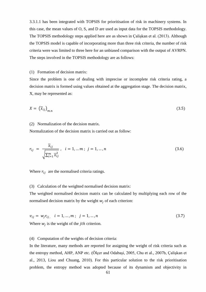
61

3.3.1.1 has been integrated with TOPSIS for prioritisation of risk in machinery systems. In

this case, the mean values of O, S, and D are used as input data for the TOPSIS methodology.

The TOPSIS methodology steps applied here are as shown in Çalişkan et al. (2013). Although

the TOPSIS model is capable of incorporating more than three risk criteria, the number of risk

criteria were was limited to three here for an unbiased comparison with the output of AVRPN.

The steps involved in the TOPSIS methodology are as follows:

(1) Formation of decision matrix:

Since the problem is one of dealing with imprecise or incomplete risk criteria rating, a

decision matrix is formed using values obtained at the aggregation stage. The decision matrix,

X, may be represented as:

𝑋 = (𝑥𝑖𝑗)𝑚.𝑛 (3.5)

(2) Normalization of the decision matrix.

Normalization of the decision matrix is carried out as follow:

𝑟𝑖𝑗 = 𝑥𝑖𝑗

√∑ 𝑥𝑖𝑗2𝑚

𝑖=1

, 𝑖 = 1,…𝑚 ; 𝑗 = 1,… , 𝑛 (3.6)

Where 𝑟𝑖𝑗 are the normalised criteria ratings.

(3) Calculation of the weighted normalised decision matrix:

The weighted normalised decision matrix can be calculated by multiplying each row of the

normalised decision matrix by the weight 𝑤𝑗 of each criterion:

𝑣𝑖𝑗 = 𝑤𝑗𝑟𝑖𝑗 , 𝑖 = 1, … ,𝑚 ; 𝑗 = 1,… , 𝑛 (3.7)

Where 𝑤𝑗 is the weight of the 𝑗𝑡ℎ criterion.

(4) Computation of the weights of decision criteria:

In the literature, many methods are reported for assigning the weight of risk criteria such as

the entropy method, AHP, ANP etc. (Ölçer and Odabaşi, 2005, Chu et al., 2007b, Çalişkan et

al., 2013, Liou and Chuang, 2010). For this particular solution to the risk prioritisation

problem, the entropy method was adopted because of its dynamism and objectivity in

62

weighting of risk criteria relative to the decision making process, as opposed to AHP and

ANP and other prior weighting methods that assign weight subjectively and independent of

the decision making process. The steps are as follows (Çalişkan et al., 2013):

Using the normalised decision matrix, the entropy value 𝑒𝑗 of 𝑗𝑡ℎ criterion is calculated as

follow:

𝑒𝑗 = −𝑘 ∑𝑟𝑖𝑗

𝑚

𝑖=1

ln 𝑟𝑖𝑗 (3.8)

Where 𝑘 =1

ln𝑚 is a constant which guarantees 0 ≤ 𝑒𝑗 ≤ 1and m is the number of failure

modes.

The objective weight for each risk criterion is then given by

𝑤𝑗 =1 − e𝑗

∑ 1 − e𝑗𝑛𝑗=1

(3.9)

(5) Determination of the positive-ideal and negative-ideal solutions.

The reference values for risk prioritisation are the positive and negative ideal solutions. The

positive ideal solution, 𝐴+, is the best value of each weighted criterion and the negative ideal

solution, 𝐴−, is the worst value of each weighted criterion and are determined as follows:

𝐴+ = {𝑣1+ , 𝑣2 ,…,

+ 𝑣𝑛+} = {(max

𝑖𝑣𝑖𝑗 |𝑗𝜖𝐼) , (min

𝑖𝑣𝑖𝑗 |𝑗𝜖𝐼′)} (3.10)

𝐴− = {𝑣1− , 𝑣2 ,…,

− 𝑣𝑛−} = {(min

𝑖𝑣𝑖𝑗 |𝑗𝜖𝐼) , (max

𝑖𝑣𝑖𝑗 |𝑗𝜖𝐼′)} (3.11)

Where 𝐼 is associated with the benefit criteria and 𝐼′ is associated with cost criteria

(6) Determination of the distance from positive-ideal and negative-ideal solutions.

The distance of each failure mode from the positive-ideal solution, 𝐷𝑖+, and from the negative-

ideal solution, 𝐷𝑖−, are evaluated, respectively as:

63

𝐷𝑖+ = √∑( 𝑣𝑖𝑗 − 𝑣𝑗

+)2

𝑛

𝑗=1

𝑖 = 1,2… .𝑚; 𝑗 = 1, 2, … , 𝑛 (3.12)

𝐷𝑖− = √∑( 𝑣𝑖𝑗 − 𝑣𝑗

− )2

𝑛

𝑗=1

𝑖 = 1,2, … ,𝑚; 𝑗 = 1,2, … , 𝑛 (3.13)

(7) Computation of the relative closeness of failure mode 𝑖 to the positive ideal solution

The relative closeness 𝑅𝐶𝑖 of each failure mode to the positive ideal solution is computed as:

𝑅𝐶𝑖 =𝐷𝑖

−

𝐷𝑖+ + 𝐷𝑖

− , 𝑖 = 1 , … ,𝑚 (3.14)

The 𝑅𝐶𝑖 value is the risk index of the failure modes. The higher the value the greater the risk

the failure mode poses to the system.

(8) Computation of mean risk of failure modes:

Finally, where data is available from multiple experts, 𝑅𝐶𝑖 values from the individuals are

averaged to obtain the mean risk of each failure mode.

3.4 Case studies

The applicability of the proposed methods for risk prioritisation of failure modes of marine

machinery systems were investigated with three case studies.

3.4.1 Case study 1

To validate the aggregation technique (averaging technique) used in this research a case

study in the literature presented by Yang et al. (2011) and Su et al. (2012) was used. The

authors used modified Dempster-Shafer evidence theory in aggregating opinions of three

experts. The methodologies of Yang et al. (2011) and Su et al. (2012) were designed to

aggregate only complete distribution criteria ratings (see Section 3.3.1.1 for a description of

complete distribution criteria ratings). In addition to this, their methodologies rely on there

64

being only a marginal difference between the risk criteria ratings from the different experts

otherwise the combination of the ratings will be zero. Therefore, in order to validate the

proposed averaging technique and allow comparison of the results, it was implemented using

the data from three experts in Table 3.2 as presented in Yang et al. (2011) and Su et al.

(2012). The methodological steps of the AVRPN technique were applied in solving the

problem in table 3.2 and the results obtained have been compared with the results obtained

from the modified Dempster-Shafer evidence theory technique as shown in Table 3.3 and

Figure 3.2.

Table 3.2: Three experts rating of 17 failure modes (Yang et al., 2011, Su et al., 2012)

65

Table 3.3: AVRPN v. D-S methods

Figure 3.2: Comparison of AVRPN with Dempster – Shafer theory method

From Figure 3.2 it can be seen that the results obtained from AVRPN closely match those

from Yang et al. (2011) (D-S method) and Su et al. (2012) (Modified D-S method). For

example, for failure modes 3, 6, 7, 10 and 11 the same RPN value was obtained from all three

methods and in the cases of failure modes 1, 2, 4, 5, 8, 12 ,14, 15 and 16 the difference in the

0

10

20

30

40

50

60

70

80

1 2 3 4 5 6 7 8 9 10 11 12 13 14 15 16 17

RP

N

Failure modes

AVRPN

D-S method

Modified D-S

66

RPN is marginal and results in no change to the ranking of the failure modes. The principal

differences occur with failure modes 9, 13 and 17 although there is a high level of similarity

between AVRPN and the modified Dempster-Shafer evidence theory method of (Su et al.,

2012) other than for failure mode 9. The sharp deviation of the D-S method RPN values for

failure modes 13 and 17 is attributed to incorrectly reported values according to Su et al.

(2012). It is obvious from the above example that the AVRPN approach is simple and robust

but it is also more flexible for real life applications as it is capable of handling not only

incomplete distribution risk criteria information but also of dealing with imprecise

distribution risk criteria data.

3.4.2 Case study 2: Application to the basic marine diesel engine

The AVRPN technique was also applied to a case study of a marine diesel engine. The marine

diesel engine was chosen because it is one of the key marine machinery systems as it provides

the power for the propulsion of the entire ship system. In addition, the marine main engine

accounts for over 45 percent of the total compensation for fault accident claims of the entire

ship system according to the survey carried out by a Swiss shipping insurance Company

(Dong et al., 2013). It is then obvious that the marine diesel engine is central to the operation,

of not only the machinery systems, but of the entire ship system powered by this type of

engine. In this case study only the basic marine diesel engine is considered while in case study

3 the entire marine diesel engine will be considered.

Ten major equipment items of the basic engine were considered including: main bearing,

piston, cylinder head and crankshaft. Each equipment item’s failure modes were examined

with the causes of failure and the effects of the failures at two levels (local and global effects)

for the different failure modes. A total of 23 failure modes were examined; a sample of these

are defined in Table 3.4 along with their causes and effects while the full table is in Appendix

A1. The risk criteria (O, S and D) values were assigned by three experts for each failure mode

through the use of an ordinal ranking scale, as shown in Table 3.1. The three experts that

participated in assigning values for criteria reached a consensus and the agreed values are

presented in Table 3.5. The three experts have both academic qualifications, with two being

PhD holders, and sea going and marine diesel engine maintenance experience over many

years.

67

Table 3.4: Sample of the FMEA for basic engine of a marine diesel engine

3.4.2.1 AVRPN: AVeraging technique and RPN analysis

The values assigned to failure modes against decision criteria in Table 3.5 were used as the

input for the AVRPN models to:

(1) Compute minimum and maximum risk criteria values:

In Table 3.5, for failure mode 1 the expert gave two incomplete rating values for 𝑥11 i.e.

Occurrence (O) to be 7:30% and 8:60%; precise rating for 𝑥12 i.e. Severity (S) to be 3 and an

68

incomplete rating for 𝑥13 i.e. Detectability (D) to be 4:70%. Since 𝑥11 had an incomplete

rating it was transformed into minimum 𝑥𝑖𝑗𝑚𝑖𝑛 and maximum 𝑥𝑖𝑗

𝑚𝑎𝑥 risk criteria ratings, using

Eq. (3.1) and Eq. (3.2) respectively.

(2) Compute mean risk criteria values:

The mean risk criterion 𝑥11 was computed using Eq. (3.3). Following the same process of

evaluation, 𝑥12 and 𝑥13 were calculated.

(3) Compute the risk (RPN) of the failure mode:

The value of RPN for failure mode 1 was obtained using equation (3.4) as follows:

𝑅𝑃𝑁1 = 7.5 𝑥 3 𝑥 4.5 = 101.25

The evaluated RPN values for the 23 failure modes and their corresponding rank are

presented in Table 3.5 and Figure. 3.3.

69

Table 3.5: Risk criteria rating, RPN values and rankings

70

Figure 3.3: Failure modes RPN values and ranking

It is obvious from Figure 3.3 that failure mode 8 has the highest RPN value with a

corresponding rank of 1, meaning its poses the greatest risk to the basic marine diesel engine.

On the other hand, failure mode 11 with the lowest RPN value and a corresponding rank of 23

poses the least risk to the system. One advantage of this methodology lies in its ability to

aggregate imprecise expert rating of risk criteria with simple averages that are very easy to

compute unlike the Dempster-Shafer theory method, data envelopment techniques and fuzzy

logic theory approaches that are more computationally intensive.

3.4.2.2 AVTOPSIS analysis

In the application of AVTOPSIS to the case study of the marine diesel engine, information

obtained from the aggregation stage was used to form the decision matrix shown in Table 3.6.

The decision matrix was normalised using Eq. (3.6) and then multiplied by the criteria

weights to obtain a weighted normalised matrix. The weighted normalised matrix is also

presented in Table 3.6. Note the weights of each criterion were evaluated using Eq. (3.6),

(3.8) – (3.9). Eq. (3.10) and (3.11) were then utilised to determine the positive ideal and

negative ideal solutions respectively. Finally, applying Eq. (3.12) – (3.14) the distance of each

failure mode to the positive-ideal solution 𝐷𝑖+ and to the negative-ideal solution 𝐷𝑖

− together

with relative closeness 𝑅𝐶𝑖 of each failure mode to the ideal solution were calculated and the

0

3

6

9

12

15

18

21

24

0

50

100

150

200

250

300

350

400

1 3 5 7 9 11 13 15 17 19 21 23

RA

NK

RP

N

Failure modes

Rank

RPN

71

results are shown in Table 3.7. The failure modes were then ranked based on 𝑅𝐶𝑖 scores; the

ranking order is also presented in Table 3.7 and Figure 3.4.

Table 3.6: Decision matrix with weighted normalised decision matrix expert 1 basic engine

72

Table 3.7: Performance index and rank

73

Figure 3.4: RCi values and rankings of 23 failure modes

From Figure. 3.4 it is clear that the second failure mode i.e. failure to lubricate the main

bearing with the highest value of 𝑅𝐶𝑖 is the best ranked and as such poses the greatest risk to

the basic engine of a marine system while failure mode 11 i.e. cracking of the crankshaft has

the lowest value of 𝑅𝐶𝑖 meaning it is the least critical failure mode of the system. It can also

be observed that failure modes 8 and 9 although ranked third and second have 𝑅𝐶𝑖 values

almost the same as that of failure mode 2 and as such the same attention should be given to all

three failure modes. This is the case because the method is subjective and any slight changes

in the input information into the model can make a significant change to the rankings.

3.4.2.3 Comparison of the methods

The failure mode risk ranking generated using the two proposed methods with risk criteria

information obtained from experts is shown in Figure 3.5. From Figure 3.5 it is obvious that

when AVRPN and AVTOPSIS are performed on the same task, the results generated may not

be the same but are very similar. For example failure modes 3, 5, 10, 11, 17 and 21 were all

given same ranking in both methods. The majority of other failure modes had a difference of

1 ranking between the methods.

According to Jahan et al. (2010) the degree of agreement between MCDM methods is

measured using the Spearman rank correlation which evaluates the sum of the squares of the

deviations between the different rankings. When the Spearman rank correlation between the

0

3

6

9

12

15

18

21

24

0.0000

0.1000

0.2000

0.3000

0.4000

0.5000

0.6000

0.7000

0.8000

1 3 5 7 9 11 13 15 17 19 21 23

Ran

k

RC

i

Failure modes

Rank

RCj

74

methods was evaluated a result of 0.9585 was obtained showing that the two methods are

strongly correlated. The implication of this is that either method can be suitable for use in

prioritisation of marine machinery systems and other engineering systems when dealing with

data that may be imprecise. However when the risk prioritisation problem involves dealing

with more than three risk criteria the AVTOPSIS method should be employed since AVRPN

is limited to three risk criteria.

Figure 3.5: Comparison of risk of failure mode ranking obtained with proposed methods.

3.4.3 Case study 3: Application to the marine diesel engine

The second case study that was used to demonstrate the applicability of the proposed

methodologies was the basic marine diesel which included components such as the piston,

crankshaft and the cam assembly. The third case study is not be limited to the basic engine but

includes other sub-systems of the marine diesel engine such as the scavenge air system,

exhaust gas system, air starting system, main lube oil system and central cooling systems. The

failure modes of the components of the various sub-systems of the marine diesel engine were

used to further illustrate the application of the proposed methodologies for risk assessment for

use in the marine industry. For the whole system, 74 failure modes were considered for

investigation, as presented in Appendix A1, together with their causes and effects. The same

experts that were used in assigning ratings for the 23 failure modes in case study 2 were also

utilised in rating the 74 failure modes of this case study. A sample of the assigned ratings is

0123456789

1011121314151617181920212223

1 2 3 4 5 6 7 8 9 10 11 12 13 14 15 16 17 18 19 20 21 22 23

Ran

k

Failure modes

AVRPN

AVTOPSIS

75

shown in Table 3.8 while the full table is presented in Appendix A2. It is worth noting that a

consensus was reached among the three experts in rating of the 74 failure modes.

Table 3.8: Sample of assigned criteria rating

3.4.3.1 AVRPN analysis

The assigned ratings against the three decision criteria; O, S and D for the 74 failure modes

were then applied as input data into the AVRPN methodology.

Firstly the expert-assigned imprecise ratings for the 74 failure modes in Table 3.8 were

aggregated using Eq. 3.1 to 3.3. The aggregated values were then used as input in Eq. 3.4 to

evaluate risk of the 74 failure modes and the results are presented in Appendix A4 and Figure

3.6. From the graph, failure mode 8 is the best ranked failure mode having the highest risk

priority number (RPN). This shows that based on this particular risk ranking methodology

failure mode 8 poses the greatest risk to the marine diesel engine. The least ranked failure

mode is failure mode 70 having the lowest value of RPN. Hence failure mode 70 poses the

least threat to the marine diesel engine.

76

Figure 3.6: Failure modes RPN values and ranking

3.4.3.2 AVTOPSIS analysis

The assigned risk ratings of the 74 failure modes aggregated using Eq. 3.1 to 3.3 were then

used to form a decision matrix, a sample of which is presented in Table 3.9 and the full matrix

is presented in Appendix A3. Next the decision criteria were normalised using Eq. 3.6. The

normalised decision matrix was then multiplied by the decision criteria weight to form the

weighted normalised matrix. In this case study the weight of the decision criteria were

determined using the entropy method modelled as Eq. (3.6), (3.8) – (3.9). The decision

criteria weights obtained were as follows; O =0.3443, S = 0.3326 and D = 0.3231. The

positive ideal and negative ideal solutions were determined using Eq. (3.10) and (3.11). The

distance of each failure mode to the positive-ideal solution, 𝐷𝑖+, and negative-ideal solution,

𝐷𝑖−, together with relative closeness, 𝑅𝐶𝑖 , of each failure mode to the ideal solution were

evaluated using Eq. (3.12) – (3.14). The graphical representation of the result of the relative

closeness of each failure mode to the ideal solution and the corresponding ranking of the 74

failure modes are shown in Figure 3.7.

0

10

20

30

40

50

60

70

80

0.00

50.00

100.00

150.00

200.00

250.00

300.00

350.00

400.00

1 3 5 7 91

11

31

51

71

92

12

32

52

72

93

13

33

53

73

94

14

34

54

74

95

15

35

55

75

96

16

36

56

76

97

17

3

Ran

k

RP

N

Failure modes

RPN

Rank

77

Table 3.9: Sample of decision matrix

Figure 3.7: RCi values and rankings of 23 failure modes

From Figure 3.7, failure mode 8 with TOPSIS performance index of 0.6707 is the best ranked

failure mode and as such possess the highest risk to the system. In terms of risk contribution

to the system this is followed by failure mode 2 ranked second with a TOPSIS performance

index (𝑅𝐶𝑖) of 0.6413 while the least contributor to the system risk is failure mode 54 having

the lowest TOPSIS performance index value of 0.2129.

0

10

20

30

40

50

60

70

80

0.0000

0.1000

0.2000

0.3000

0.4000

0.5000

0.6000

0.7000

0.8000

1 4 7 10 13 16 19 22 25 28 31 34 37 40 43 46 49 52 55 58 61 64 67 70 73

Ran

k

RC

j

Failure modes

RCj Rank

78

3.4.3.3 Comparison of methods

The failure mode rankings generated from utilising the two techniques; AVRPN and

AVTOPSIS are presented in Figure 3.8.

Figure 3.8: Comparison of proposed methods

From Figure 3.8 it can be seen that the majority of failure modes are ranked the same by the

two methods while a few others have a rank difference of one between them. The Spearman

rank correlation coefficient between AVRPN and AVTOPSIS was evaluated and a value of

0.9000 was obtained. With the strong correlation between the two methods it can be

suggested that the two techniques can be used individually or in combination for risk

prioritisation.

3.5 Summary

In this Chapter some of the limitations of the conventional FMEA method were addressed

using two approaches for risk prioritisation; AVRPN and AVTOPSIS. Both methods utilise a

novel approach using averages without resorting to specialised software or the need for the

decision maker to have knowledge of specialised programming concepts, in aggregating

multiple experts’ diverse information that may be imprecise or incomplete. The AVRPN

technique was proven to match almost completely with the Yang et al. (2011) and Su et al.

(2012) modified Dempster-Shafer method when it was applied to a complete distribution risk

criteria problem from the literature. It was also demonstrated that the approach is simple yet

0

10

20

30

40

50

60

70

80

1 3 5 7 9 11 13 15 17 19 21 23 25 27 29 31 33 35 37 39 41 43 45 47 49 51 53 55 57 59 61 63 65 67 69 71 73

Ran

k

Failure modes

AVRPN AVTOPSIS

79

robust and capable of dealing with imprecise distribution risk criteria problems which the

modified Dempster-Shafer theory technique is incapable of solving. Comparison between the

two proposed methods (AVRPN and AVTOPSIS) revealed that both techniques can be

suitable for use in risk prioritisation jointly or independently as the results generated by both

methods were very similar. However the AVTOPSIS method is capable of incorporating

more than three risk criteria unlike AVRPN. Although both techniques have been developed

for risk prioritisation, they can easily be modified to address other multi-decision engineering

problems such as maintenance strategy selection problems. Finally another novel aspect in the

chapter, to the best of the author’s knowledge, is the fact that this is the first application of

TOPSIS, an MCDM tool, in analysing a problem involving imprecise information from

multiple experts.

80

Chapter 4 Risk Assessment using Compromise Solution Method

4.1 Introduction

In Chapter 3 two techniques were proposed for prioritisation of the risk of failure modes of

machinery systems. As stated in Chapter 3, AVRPN addresses only a single limitation of the

classical FMEA. AVTOPSIS which is the combination of the averaging technique and

TOPSIS has an advantage over AVRPN in that it is capable of addressing more challenges of

the classical FMEA. TOPSIS is a compromise solution methodology that is based on the fact

that the best alternative is the one closest to the positive ideal solution and farthest from the

negative ideal solution, however when compared to other compromise solution methods,

more computational effort is required in evaluating the positive and negative ideal solutions

(Rao, 2008). Other limitations of the TOPSIS technique are (Opricovic and Tzeng, 2004): (1)

the optimum solution is not close to the ideal solution when the ideal solution has value of 1

and (2) the relative distance between positive ideal and negative ideal is not considered in the

evaluation process which negatively affects the decision making process.

In order to further eliminate or mitigate the limitations of the classical FMEA, two Multi-

Criteria Decision Making (MCDM) tools are proposed as alternatives to the classical FMEA.

The proposed MCDM tools are Vlsekriterijumska Optimizacija Ikompromisno Resenje,

meaning: Multicriteria Optimization and Compromise Solution (VIKOR) and Compromise

Programming (CP).. Utilising these two MCDM techniques, which have successfully been

applied in solving problems other than risk prioritisation, will allow more decision criteria and

flexible decision criteria weights to be use in prioritising risk of failure modes which will

therefore result in the risk of failure mode being more effectively prioritised or ranked. In

order to enhance the capability of the two MCDM techniques in addressing the limitations of

the classical FMEA, the averaging technique introduced in Chapter 3 has been integrated with

the two proposed MCDM techniques. This allows the proposed compromise solution methods

to use precise and /or imprecise ratings from experts as input. Thus the use of the averaging

technique in the MCDM tools will eliminate the limitation of the classical FMEA of the

inability to aggregate imprecise criteria ratings from experts. Furthermore two objective

weighting techniques are incorporated into the methodology which is a break away from the

use of subjective weighting techniques that may biasedly influence the decision making

81

process. The suitability and applicability of the proposed methodologies in risk ranking of

failure modes of the marine diesel engine are investigated through case studies.

The chapter is organised as follows: Section 4.2 presents a review of MCDM tools and

Section 4.3 presents the proposed methodology for risk prioritisation. In Section 4.4 three

case studies are presented for illustration of the proposed technique. Finally conclusions are

presented in Section 4.5.

4.2 Review of MCDM tools and their relevance to the Marine industry

As previously stated in Chapter 3, the classical FMEA technique has limitations and in order

to enhance its capability and reduced these flaws, various MCDM techniques have been

applied in the literature.

Braglia (2000) proposed the Analytical Hierarchical Process (AHP) technique as an

alternative to RPN in the FMEA system. With this method, a three-level hierarchy was

formed with the top level representing the main objective of fault cause selection, the

intermediate level representing the four risk criteria, O, S, D and economic cost and the

lowest level representing the alternative causes of failures. With this, a series of pairwise

comparison matrices was formed and evaluated to obtain the weight of risk criteria and local

priorities of the possible causes of failure with respect to O, S, D and economic cost. The

aggregation technique in AHP was used to synthesize the local priorities of causes of failure

into global priorities based on which possible cause of failure was ranked. Carmignani (2009)

used a similar approach to that of Braglia (2000) and in the methodology of the former, a new

profitability calculation technique was introduced in place of economic cost for risk

prioritisation of an electro-injector, a fuel system component. However the use of AHP has

been criticised due to its use of an unbalanced scale of judgement and its inadequacy in

addressing risk criteria ratings that may be uncertain and imprecise in the pairwise

comparison process (Deng, 1999, Ilangkumaran and Kumanan, 2009). Furthermore, the AHP

technique is performed on problems with 2 to 15 risk criteria and if a problem with more than

15 decision criteria is to be considered some other technique is required to initially reduce the

number of risk criteria (Vidal et al., 2011a).

Maheswaran and Loganathan (2013) proposed a hybrid MCDM technique as an alternative to

RPN in the traditional FMEA system. The technique was based on integration of AHP and the

82

Preference Ranking Organisation METHod for Enrichment Evaluation (PROMETHEE). The

authors used AHP to determine the weight of each risk factor and used PROMETHEE for

prioritising the failure modes. The methodology was illustrated by applying it to prioritising

failure modes of a boiler system in the tyre manufacturing industry. Ayadi et al. (2013)

presented a multi-criteria failure mode and effects analysis approach based on PROMETHEE

for prioritising potential failure modes applied to manufacturing of a gas treatment plant.

Moreira et al. (2009) proposed PROMETHEE in the ranking of equipment failure modes.

PROMETHEE results in poor structuring of problems compared to AHP and when more than

seven risk criteria are used it becomes difficult to obtain a view of the problem thereby

making the evaluation process very complicated (Macharis et al., 2004).

Seyed-Hosseini et al. (2006) proposed a methodology referred to as Decision Making Trial

and Evaluation Laboratory (DEMATEL) as alternative to RPN in the classical FMEA for

prioritisation of failure modes. With this approach, failure modes are prioritised based on

severity of effect and direct/indirect relationships between them. However one of the

challenges of DEMATEL is that it requires a lot of computational effort and according to

Shaghaghi and Rezaie (2012) it cannot address the limitations of the traditional RPN method

especially in a system where each cause of failure is linked to a single failure mode; the

results obtained by both methods are the same.

Sachdeva et al. (2009b) proposed an integrated Shannon’s entropy method with TOPSIS

which enhanced the FMEA for risk assessment. Six criteria of O, D, maintainability, spare

parts availability, economic safety and economic cost were considered for risk prioritisation.

An illustration was given with the application to the digester of a paper manufacturing plant in

India. Braglia et al. (2003) also used TOPSIS under a FUZZY environment for risk

prioritisation of a foaming machine of a refrigerator production line. The use of TOPSIS,

especially in the fuzzy environment, is computationally intensive and that may make the

proposed technique unattractive to the maintenance practitioner.

From the above review and according to Maheswaran and Loganathan (2013), only limited

publications are available using MCDM techniques in enhancing the classical FMEA

evaluation methodology. Moreover the few MCDM techniques employed so far all have one

limitation or another. Hence there is need for an alternative MCDM technique devoid of the

limitations of the MCDM techniques applied by other researchers and which will sufficiently

address the challenges of FMEA especially for the marine environment. On this basis, two

83

MCDM compromise solution methods are proposed; VIKOR and CP as alternatives to the

standard RPN calculation of the FMEA system.

4.3 Proposed hybrid MCDM risk analysis tool for use on marine machinery systems

The proposed enhanced FMEA based on the averaging technique integration with VIKOR

and CP is presented in Figure 4.1.

Figure 4.1: Flow chart of proposed hybrid MCDM risk analysis tool

The methodological steps of the enhanced FMEA model are briefly discussed as follows:

Steps (a), (b) and (c): The activities here involve formation of a team of experts who

determine the particular system to be investigated. The failure modes of the system are then

determined through brainstorming and the use of techniques such as root cause analysis and

Fault Tree Analysis (FTA)

84

Step (d) Aggregation of imprecise rating: If imprecise ratings are assigned by experts to

failure modes against decision criteria these are aggregated into precise ratings using the

averaging technique discussed in Chapter 3.

Step (e) Determination of criteria weight: The weight of each of the decision criteria is

determined objectively by employing two techniques; the entropy method and the variance

method. The results from the two techniques are compared in order to ascertain the

relationship between both techniques.

Step (f) Ranking of failure modes: VIKOR and CP are both applied individually in place of

the RPN of the classical FMEA to determine the risk of the failure modes. This is carried out

by using the performance index of both techniques to measure the performance of each failure

mode and based on the index, the failure modes are ranked.

Step (g) the ranking obtained from both methods are compared.

4.3.1 Criteria weighting methods

The determination of the weight of risk criteria is a key factor in risk prioritisation because of

the impact of the risk criteria in the final ranking of the failure modes of a system. In the

literature, many methods are available for assigning weight of attributes; among these

techniques is the use of the entropy method (Çalişkan et al., 2013, Jee and Kang, 2000,

Shanian and Savadogo, 2006). The statistical variance method has also been used by some

authors (Rao and Patel, 2010, Nirmal, 2013). Subjective methods such as AHP, Weighted

Evaluation Technique (WET), the Points method and the digital logic method have also been

employed (Rao, 2007).

For this chapter, the entropy method and the statistical variance method were adopted because

these are objective techniques of weighting criteria there-by reducing personal bias in the

overall decision making process which may influence purely subjective methods. Moreover

they have been applied individually by previous researchers in dealing with similar problems

as detailed above. However one of the objectives of this chapter is to compare both methods

in order to determine suitability and applicability for marine machinery systems.

85

4.3.1.1 Entropy method

The steps of the Entropy method are as follows (Çalişkan et al., 2013):

(1) The decision matrix is formed. The decision matrix is produced using the values of 𝑥𝑖𝑗

obtained in the data aggregation stage as follows:

𝑋 = (𝑥𝑖𝑗)𝑚 .𝑛 ( 4.1)

(2) The decision matrix is then normalised:

𝑝𝑖𝑗 =𝑥𝑖𝑗

∑ 𝑥𝑖𝑗𝑚𝑖=1

, 𝑖 = 1,2, … ,𝑚; 𝑗 = 1,2, … , 𝑛 (4.2 )

Where 𝑝𝑖𝑗 is the normalised matrix.

(3) The entropy value 𝑒𝑗 of each criterion is then determined:

𝑒𝑗 = −𝑘 ∑𝑝𝑖𝑗

𝑚

𝑖=1

ln 𝑝𝑖𝑗 (4.3)

Where 𝑘 =1

ln𝑚 is a constant which guarantees 0 ≤ 𝑒𝑗 ≤ 1

(4) Finally the objective weight 𝑤𝑗𝑒 for each attribute is given by:

𝑤𝑗𝑒 =

1 − e𝑗

∑ 1 − e𝑗𝑛𝑗=1

(4.4)

4.3.1.2 Statistical variance method

In determining the weight of risk criteria, the steps are as follows (Rao and Patel, 2010,

Nirmal, 2013):

(1) The first step is the normalisation of the decision matrix in equation (4.1) as follows:

𝑟𝑖𝑗 =𝑥𝑖𝑗

∑ 𝑥𝑖𝑗𝑚𝑖=1

, 𝑖 = 1,2, … ,𝑚; 𝑗 = 1,2, … , 𝑛 (4.5)

Where 𝑟𝑖𝑗 is the normalised matrix.

86

(2) Next the variance of each risk criterion is evaluated as follows:

𝑉𝑗 =1

𝑚[∑(𝑟𝑖𝑗 − 𝑟𝑖𝑗)

2𝑚

𝑖

] (4.6)

Where 𝑟𝑖𝑗 is the mean value of 𝑟𝑖𝑗

𝑉𝑗 is the variance of each risk criterion.

(3) Finally the weight of each risk criterion is calculated as follows:

𝑤𝑗𝑣 =

𝑉𝑗

∑ 𝑉𝑗𝑛𝑗

(4.7)

Where 𝑤𝑗𝑣 is the weight of each criterion

4.3.2 Failure mode ranking tools

The two MCDM techniques; VIKOR and CP proposed for the ranking of the failure modes of

marine machinery systems are discussed next.

4.3.2.1 VIKOR method

The VIKOR method was developed by S. Opricovic in 1979 (Opricovic, 1998) and is defined

as a multi-criteria decision making tool which focuses on ranking and selecting a compromise

solution from a set of alternatives with reference to conflicting criteria. The compromise

solution is obtained using a ranking index based on a measure of closeness to the positive

ideal solution (Opricovic, 1998, Opricovic and Tzeng, 2004). The key concept of the method

lies in defining the positive and negative ideal solutions. While the positive and negative ideal

solutions are defined as the alternatives with the highest and lowest values respectively with

reference to risk criteria (Chu et al., 2007a), the optimum or compromise solution is defined

as the alternative closest to the positive ideal solution and farthest from the negative ideal

solution. The VIKOR method has been used by many authors in resolving different multi-

criteria decision problems in literature; in the selection of industrial robots (Nirmal, 2013),

selection of vendors (Hsu et al., 2012), an equipment selection problem for mining operations

(Aghajani Bazzazi et al., 2011) and material selection problems (Liu et al., 2013, Chatterjee et

al., 2009, Rao, 2008, Çalişkan et al., 2013, Anojkumar et al., 2014).

87

The use of VIKOR in this context as an alternative to the RPN calculation of the FMEA

system is based on the following considerations:

(1) The classical FMEA is limited to use of only three decision criteria; O, S and D for

prioritisation of the risk of failure modes of marine machinery systems. However the use of

VIKOR in place of the RPN of the classical FMEA allows the inclusion of other important

decision criteria such as economic cost and profitability.

(2) Failure modes are better ranked and more clearly distinguished from one another using

VIKOR than RPN of the classical FMEA system. This is because with the use of RPN in the

classical FMEA, different combinations of O, S and D may result in having the same RPN

values for different failure modes but the risks in the practical sense may not be the same. The

aggregation technique of VIKOR combines the decision criteria; O, S and D in a systematic

manner such that it is almost impossible to have the same value for risk.

(3) VIKOR allows varying decision criteria weights to be applied in evaluating risk as

opposed to classical FMEA that assumes equal weight for decision criteria.

(4) The integration of the averaging technique into VIKOR allows both precise and

imprecise data to be applied in evaluating risk of failure modes whereas classical FMEA

relies only on precise data from experts.

(5) No application of VIKOR techniques is reported in the literature for risk assessment of

marine machinery systems and other related systems, so applying this MCDM technique

which has successfully been used in solving other multi-criteria decision problems will be a

positive step for the marine industry.

(6) Less computational effort is required than for the TOPSIS method (Nirmal, 2013, Rao,

2008, Carpinelli et al., 2014) and other MCDM techniques that have previously been used by

other authors in risk prioritisation of failure modes. Moreover the limitation of the TOPSIS

methodology is with respect to its inability to consider relative distance from the positive

ideal and negative ideal solutions which may be addressed through the VIKOR method

(Anojkumar et al., 2014).

The basic steps involved in the VIKOR methodology are as follows (Çalişkan et al., 2013,

Sayadi et al., 2009):

(1) Determination of the best and worst values for each criterion.

88

Using the decision matrix in Eq. (4.1) the best and worst values for each criterion are

determined as follows:

𝑥𝑗+

= max𝑖

𝑥𝑖𝑗, 𝑥𝑗−

= min𝑖

𝑥𝑖𝑗 ( 4.8)

Where,

𝑥𝑗+ is the best value for the 𝑗𝑡ℎ criterion, and

𝑥𝑗−

is the worst value for the 𝑗𝑡ℎ criterion.

(2) Computation of the utility measure and regret measure for each failure mode is as

follows:

𝑆𝑖 = ∑𝑤𝑗

𝑛

𝑗=1

(𝑥𝑗+

− 𝑥𝑖𝑗) (𝑥𝑗+

− 𝑥𝑗−) (4.9) ⁄

𝑅𝑖 = max𝑗

𝑜𝑓 [𝑤𝑗 (𝑥𝑗+

− 𝑥𝑖𝑗) (𝑥𝑗+

− 𝑥𝑗−)⁄ ] (4.10)

Where

𝑤𝑗 is the weight of 𝑗𝑡ℎ criterion, which represents the relative importance of the criterion.

𝑆𝑖 is the utility measure

𝑅𝑖 is the regret measure

(3) Computation of the VIKOR index value 𝑄𝑖 ,

This is expressed as:

𝑄𝑖 = 𝑣 (𝑆𝑖 − 𝑆+) (𝑆− − 𝑆+)⁄ + (1 − 𝑣)(𝑅𝑖 − 𝑅+) /(𝑅− − 𝑅+) (4.11)

Where

𝑆+ = max𝑖

[(𝑆𝑖) , 𝑖 = 1,2, … ,𝑚]

𝑆− = min𝑖

[(𝑆𝑖) , 𝑖 = 1,2, … ,𝑚]

𝑅+ = max𝑖

[(𝑅𝑖) , 𝑖 = 1,2, … ,𝑚]

89

𝑅− = min𝑖

[(𝑅𝑖) , 𝑖 = 1,2, … ,𝑚]

𝑣 represents the weight of the decision making strategy of the maximum group utility which

is usually set at 0.5 although it can take any value from 0 to 1 (Çalişkan et al., 2013).

However according to (Vahdani et al., 2010, Çalişkan et al., 2013) the compromise can be

selected with “voting by the majority” (𝑣 > 0.5), with “consensus” (𝑣 ≈ 0.5), or with “veto”

(𝑣 < 0.5).

(4) The ranking of failure modes is based on the VIKOR index 𝑄𝑖 value and the smaller the

value the higher the rank is and the greater the risk that it poses to the system. The value of 𝑄𝑖

represents the individual expert performance index rating. However if information is available

from multiple experts the values of individual experts is averaged.

4.3.2.2 Compromise Programming (CP)

Compromise Programming was proposed by Po-lung Yu and Milan Zeleny in 1973 (Zeleny,

1982) and has since been used by different authors in solving various multi-attribute decision

problems. The objective is to produce a solution that is closest to the ‘ideal’ solution which is

measured in terms of comparing distances of various points to a reference point (the ideal

point). The optimal solution is the one with the shortest distance to the ideal point. CP has

been applied in the following areas: Bilbao-Terol et al. (2006) presented a Fuzzy CP

technique for portfolio selection; Diaz-Balteiro et al. (2011) used the CP technique in the

ranking of seventeen European countries evaluated in terms of the sustainability of the

European paper industry; Tiwari et al. (1999) utilised CP in selecting optimum cropping

pattern using several criteria such as land suitability, energy output/input, water requirements

and environmental cost and Phua and Minowa (2005) presented a geographical information

system (GIS)- based CP technique for forest conservation planning. Having been successfully

applied in solving other problems elsewhere this chapter uses the technique to solve the risk

prioritisation problem in the marine environment.

The use of CP as an alternative to the RPN calculation of the FMEA system is based on the

following consideration:

90

(1) CP is capable of incorporating more than three risk criteria, unlike RPN, for evaluating

risk of failure modes of marine machinery systems.

(2) The relative importance of different risk criteria is taken into consideration in the risk

analysis process unlike RPN which assumes equal weight for all risk criteria.

(3) The incorporation of the averaging technique into CP makes it possible for CP to

allow the use of imprecise data for risk of failure mode evaluation as opposed to the classical

FMEA that is limited to the use of precise data.

(4) The computational effort and time required in evaluating the CP method is far less

than that of other MCDM techniques. In support of this claim Marler and Arora (2004) and

Carpinelli et al. (2014) postulated that the CP method can effectively be used when reduced

computational effort is a strict requirement.

The basic steps involved in this methodology are as follows:

(1) Determination of the positive ideal solution 𝑥𝑗+ and the negative ideal solution 𝑥𝑗

−for

the 𝑗𝑡ℎ criterion using Eq. 4.8. These are then used as input values in the risk prioritisation

index 𝑑𝑝𝑖

(2) Computation of the risk prioritisation index 𝑑𝑝𝑖

𝑑𝑝𝑖 = [∑𝑤𝑗𝑝 |

𝑥𝑗+

− 𝑥𝑖𝑗

𝑥𝑗+

− 𝑥𝑗−|

𝑝𝑛

𝑗

]

1𝑃

(4.12)

Subject to 1 ≤ 𝑝 ≤ ∞

Where risk prioritisation index 𝑑𝑝𝑖 represents the distance of failure mode 𝑖 (alternative 𝑖 )

from the ideal solution and p is the distance parameter which is used in compensating for

deviation from the ideal solution point. In the case of risk prioritisation, the smaller the value

of 𝑑𝑝𝑖 the higher the risk a failure mode possess to the system.

It is worth noting that both methods proposed are compromise solution methods. In fact Eq.

(4.9) and (4.10) of the VIKOR method were derived from equation (4.12) when p values are

set at 1 and ∞ respectively (Rao, 2008, Sayadi et al., 2009). However the key interest in the

CP method in this context is to compare results obtained, with those of VIKOR to identify

whether the methods can be used jointly or independently. The value of p was set at 2 for the

CP method because this is the standard value used in the literature (Zeleny, 1982, Phua and

Minowa, 2005).

91

4.4 Case studies

4.4.1 Case study 1: Application to the boiler of a tyre manufacturing plant

To validate the two proposed methodologies a boiler failure mode ranking problem that

Maheswaran and Loganathan (2013) solved with the PROMETHEE method was considered.

The authors identified ten failure modes using “What-if analysis” and generated a failure

report of the system. The identified failure modes were assigned precise ratings for each of

the four risk criteria Severity(S), Occurrence (O), Detection (D) and Protection (P) by

different experts, with each of the expert ratings forming an individual decision matrix. The

average of the individual decision matrices is shown in Table 4.1 which was then normalised;

the result is shown in Table 4.2.

Table 4.1: Failure modes of a boiler system and corresponding decision matrix (Maheswaran

and Loganathan, 2013)

92

Table 4.2: Normalised Decision matrix (Maheswaran and Loganathan, 2013)

4.4.1.1 VIKOR method analysis

From Table 4.2 the positive ideal and negative ideal solutions of all the risk criteria were

determined using Eq. 4.8. The relative weights of criteria are then required. For the purpose

of comparison of this proposed methodology with the PROMETHEE method of Maheswaran

and Loganathan (2013), criteria weights evaluated by these authors using AHP techniques

were used. The criteria weights assigned were 0.4996, 0.2884, 0.0655 and 0.1465 for Severity

(S), Occurrence (O), Detection (D) and Protection (P) respectively. Knowing the weight of

risk criteria, the distance of each failure mode from the positive ideal solution was then

calculated firstly based on utility measure using Eq. (4.9) and secondly based on regret

measure using Eq. (4.10). The VIKOR index 𝑄𝑖 was then calculated using Eq. (4.11) and

based on the result, the failure modes were ranked. The results of 𝑄𝑖 for each of the failure

modes and their corresponding rankings are presented in Table 4.3.

93

Table 4.3: Si, Ri and Qi and corresponding Rank of a boiler system

From Table 4.3, failure mode 2 is the most significant failure mode having the lowest 𝑄𝑖

value meaning it poses the highest risk to the boiler system. On the other hand, failure mode 3

having the highest 𝑄𝑖 value is the least significant of the 10 failure modes of the boiler system

considered. The implication is that failure mode 3 has the lowest risk contribution to the

system and as such it should attract the least attention while the greatest attention should be

paid to failure mode 2.

4.4.1.2 Compromise Programming

For the Compromise Programming method, values of the best and worst solutions were

obtained by applying Eq. (4.8) to the normalised decision matrix in Table 4.2. The values

generated were used as input into Eq. (4.12) to evaluate the risk index of the CP method. The

index values of the ten failure modes of the boiler system together with their rankings are

presented in Table 4.4.

94

Table 4.4: dp values and rank

From Table 4.4 it obvious that the highest ranked failure mode is number 2 having the lowest

dpi values and the lowest ranked is failure mode 5.

4.4.1.3 Comparison of the two methods

Table 4.5 and Figure 4.2 show comparisons of the results obtained by the two proposed

compromise solution methods with the results generated by the Maheswaran and Loganathan

(2013) PROMETHEE based methodology.

Table 4.5: Comparison of methods

95

Figure 4.2: Comparison of methods

Table 4.6: Spearman’s rank correlation coefficient

From Figure 4.2 and Table 4.5 it can be seen that all three ranking methods; VIKOR, CP and

PROMETHEE assigned the top rank to failure mode 2 (feed water pump failure). There is

absolutely no doubt that failure mode 2 is the most critical failure mode of the boiler system.

Other failure modes assigned the same ranking by the three methods are failure mode 7 and 9.

From Table 4.6, the high Spearman’s rank correlation coefficient between CP and

Maheswaran and Loganathan (2013) rankings and between VIKOR and Maheswaran and

Loganathan (2013) of 0.9758 and 0.9626 respectively, again validated the proposed

methodologies. The compromise solution methods applied in this study demand less

computational effort and time compared to the PROMETHEE method and yet produce very

similar outputs. Also the Maheswaran and Loganathan (2013) methodology can only be

applied to exact or precise data from experts but the methodology proposed in this paper is

capable of solving system problems involving both precise and imprecise information from

experts.

0

1

2

3

4

5

6

7

8

9

10

1 2 3 4 5 6 7 8 9 10

Ran

k

Failure modes

VIKOR

CP

Maheswaran

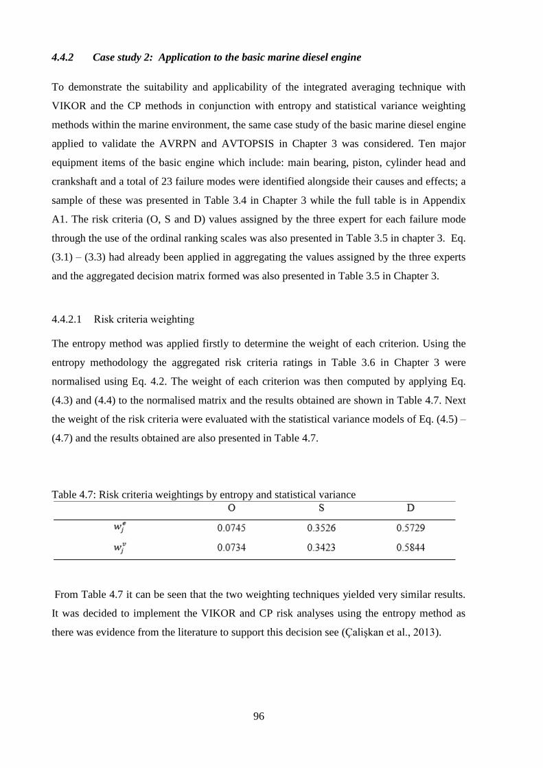
96

4.4.2 Case study 2: Application to the basic marine diesel engine

To demonstrate the suitability and applicability of the integrated averaging technique with

VIKOR and the CP methods in conjunction with entropy and statistical variance weighting

methods within the marine environment, the same case study of the basic marine diesel engine

applied to validate the AVRPN and AVTOPSIS in Chapter 3 was considered. Ten major

equipment items of the basic engine which include: main bearing, piston, cylinder head and

crankshaft and a total of 23 failure modes were identified alongside their causes and effects; a

sample of these was presented in Table 3.4 in Chapter 3 while the full table is in Appendix

A1. The risk criteria (O, S and D) values assigned by the three expert for each failure mode

through the use of the ordinal ranking scales was also presented in Table 3.5 in chapter 3. Eq.

(3.1) – (3.3) had already been applied in aggregating the values assigned by the three experts

and the aggregated decision matrix formed was also presented in Table 3.5 in Chapter 3.

4.4.2.1 Risk criteria weighting

The entropy method was applied firstly to determine the weight of each criterion. Using the

entropy methodology the aggregated risk criteria ratings in Table 3.6 in Chapter 3 were

normalised using Eq. 4.2. The weight of each criterion was then computed by applying Eq.

(4.3) and (4.4) to the normalised matrix and the results obtained are shown in Table 4.7. Next

the weight of the risk criteria were evaluated with the statistical variance models of Eq. (4.5) –

(4.7) and the results obtained are also presented in Table 4.7.

Table 4.7: Risk criteria weightings by entropy and statistical variance

From Table 4.7 it can be seen that the two weighting techniques yielded very similar results.

It was decided to implement the VIKOR and CP risk analyses using the entropy method as

there was evidence from the literature to support this decision see (Çalişkan et al., 2013).

97

4.4.2.2 VIKOR method analysis

The positive ideal solution f+ and the negative ideal solution f - were determined from the

decision matrix in Table 3.6 in Chapter 3 using Eq. (4.8). The distance of each failure mode

from the positive ideal solution was then calculated based on utility measure 𝑆𝑖 and regret

measure 𝑅𝑖 using Eq. (4.9) and (4.10) respectively. The VIKOR index values, 𝑄𝑖 , were then

evaluated for the various failure modes by subtituting values of 𝑆+, 𝑆−, 𝑅+ , 𝑅− and 𝑣 into

Eq. (4.11). The failure modes were ranked based on the VIKOR index values. The results of

the 𝑄𝑖 values of the failure modes together with the rankings are presented in Table 4.8 and

Figure 4.3.

Table 4.8: VIKOR index Qi of failure modes and rankings

98

Figure 4.3: Qi values of 23 failure modes of marine diesel engine and corresponding rankings

From Figure 4.3, it is clear that failure mode 2 is the one with the lowest value of 𝑄𝑖 and thus

is ranked number one among the 23 failure modes of the marine diesel engine. In terms of risk

impact on the system, its poses the highest risk to the marine diesel engine. On the other hand

failure mode 11 which has the highest value of 𝑄𝑖 is ranked number 23 among the 23 failure

modes and thus poses the least risk to the system.

4.4.2.3 CP method analysis

Applying Eq. (4.8) to the decision matrix in Table 3.6, the values of 𝑥𝑗+, 𝑥𝑗

− were obtained

and used as inputs to Eq. (4.12) to obtain the risk prioritisation index 𝑑𝑝 of the CP technique.

The risk prioritisation index 𝑑𝑝 values of the 23 failure modes together with the rankings are

presented in Table 4.9 and Figure 4.4.

0

5

10

15

20

25

0.0000

0.1000

0.2000

0.3000

0.4000

0.5000

0.6000

0.7000

0.8000

0.9000

1.0000

1 3 5 7 9 11 13 15 17 19 21 23

Ran

k

Qi

Failure modes

Qi

Rank

99

Table 4.9: dp of failure modes and ranking

Figure 4.4: dp values of 23 failure modes and corresponding ranking.

0

5

10

15

20

25

0.0000

0.0500

0.1000

0.1500

0.2000

0.2500

0.3000

0.3500

0.4000

0.4500

0.5000

1 3 5 7 9 11 13 15 17 19 21 23

Ran

k

dp

Failure modes

dp

100

It is obvious from Figure 4.4 that failure mode 2 has the lowest value of 𝑄𝑖, thus it is ranked

number one among the 23 failure modes. Based on this methodology, it is the most critical

failure mode in the system and, as such, greater attention should be paid to it to mitigate the

effect on the system. Failure mode 11 is again the one with the highest value of 𝑄𝑖, thus the

lowest ranked among the 23 failure modes.

4.4.2.4 Comparison of the ranking of the proposed methods with TOPSIS and AVTOPSIS

In order to validate the proposed methodologies, the results obtained from them together with

the results obtained by solving the same problem with the standard TOPSIS technique and

results obtained by AVTOPSIS in Chapter 3 were compared as shown in Figure 4.5.

Figure 4.5: Comparison of rankings obtained with MCDM methods

Table 4.10: Spearman’s rank correlation between methods

From Figure 4.5 failure modes 2, 7, 8, 9, 11, 12, 13 14, 16, 20 and 22 representing about 50%

of the total failure modes are ranked the same for three methods; VIKOR, CP and TOPSIS

0

5

10

15

20

25

1 2 3 4 5 6 7 8 9 10 11 12 13 14 15 16 17 18 19 20 21 22 23

Ran

k

Failure modes

VIKOR

CP

TOPSIS

AVTOPSIS

101

while the majority of the others have a difference of one place between failure modes.

However the TOPSIS method involves more computational effort. The gap in the results

obtained from AVTOPSIS as compared to the other three methods is as a result of the

different normalisation technique used in the entropy method in obtaining risk prioritisation

criteria weight. While for VIKOR, CP and TOPSIS the summation of the experts’ assigned

risk criteria values was used in the normalisation process in the entropy method for obtaining

criteria weight, the square root of the summation of the square values of risk criteria assigned

by experts’ was applied in the normalisation technique used in the entropy methodology in

obtaining criteria weight for the AVTOPSIS. This resulted in different risk criteria weights

used for AVTOPSIS and the deviation in rankings obtained using the technique from the three

other techniques. This then shows that criteria weights used as input in the risk prioritisation

methodology have a very strong influence in the ranking outcome. This makes the process of

evaluating criteria weight a very important and critical subject.

The Spearman rank correlations between VIKOR, CP and TOPSIS and AVTOPSIS were

evaluated and the results are shown in Table 4.10. From Table 4.10 the near perfect

Spearman rank correlations between VIKOR and CP; VIKOR and TOPSIS; CP and TOPSIS

of 0.9931, 0.9901 and 0.9862 respectively, shows the viability and validity of the two

proposed methods for prioritising risk of failure mode of a marine machinery system or any

other related systems. The Spearman rank correlation coefficient between rankings of VIKOR

and AVTOPSIS; CP and AVTOPSIS; and TOPSIS and AVTOPSIS of 0.7757, 0.7520 and

0.7213 respectively show that AVTOPSIS is also strongly related with VIKOR, CP and

TOPSIS and this further shows the viability of the proposed methodologies.

4.4.3 Case study 3: Application to a marine diesel engine

The case study of the marine diesel engine which includes all of the systems of the marine

diesel engine such as the basic engine, main lube oil system and the scavenge air system was

previously described in Section 3.4.3 in Chapter 3. The values assigned by experts using the

ordinal scale to the 74 failure modes identified for the systems as well as the resulting

aggregated decision matrix have also already been presented in Table 3.8 and 3.9 respectively

in Chapter 3. The application of the VIKOR and CP for analysis of this data is discussed next.

102

4.4.3.1 VIKOR method analysis

Applying Eq.4.8 to Table 3.9, the positive ideal solution f+ and the negative ideal solution f -

were determined. The distance of each failure mode from the positive ideal solution was then

calculated based on utility measure 𝑆𝑖 and regret measure 𝑅𝑖 using Eq. (4.9) and (4.10)

respectively. The VIKOR index values, 𝑄𝑖 , were then evaluated for the various failure modes

by subtituting values of 𝑆+, 𝑆−, 𝑅+ , 𝑅− and 𝑣 into Eq. (4.11). Based on the VIKOR index

values the failure modes were ranked. The results of the 𝑄𝑖 values of the failure modes

together with the rankings are presented in Figure 4.6. From the result, failure mode 71 is

ranked 1 having the lowest performance index i.e. 0.0234 and as such the failure mode

contributed the highest risk to the system. The failure mode that poses the least risk to the

system is failure mode 54 with a ranking of 74 and having the highest performance index

value.

Figure 4.6: Qi values of 78 failure modes and corresponding rankings

4.4.3.2 CP method analysis

The values of 𝑥𝑗+, 𝑥𝑗

− were obtained by applying Eq. (4.8) to the decision matrix in Table

3.9 and then used as inputs to Eq. (4.12) to obtain the risk prioritisation index 𝑑𝑝 of the CP

0

10

20

30

40

50

60

70

80

0.0000

0.2000

0.4000

0.6000

0.8000

1.0000

1.2000

1 3 5 7 91

11

31

51

71

92

12

32

52

72

93

13

33

53

73

94

14

34

54

74

95

15

35

55

75

96

16

36

56

76

97

17

3

Ran

kQi

Failure modes

Qi

Rank

103

technique. The risk prioritisation index 𝑑𝑝 values of the 74 failure modes together with the

rankings are presented in Figure 4.7.

Figure 4.7: dp values of 74 failure modes and corresponding ranking

4.4.3.3 Comparison of the ranking of the proposed MCDM methods with AVRPN,

AVTOPSIS and TOPSIS

To further determine the applicability of the two proposed MCDM compromise techniques

the results obtained from their analysis were compared with those of ARPN, AVTOPSIS and

the standard TOPSIS. The ranking comparison of the two proposed methods with

AVTOPSIS, AVRPN and TOPSIS are shown in Figure 4.8 a, b &c.

0

10

20

30

40

50

60

70

80

0.0000

0.1000

0.2000

0.3000

0.4000

0.5000

0.60001 3 5 7 9

11

13

15

17

19

21

23

25

27

29

31

33

35

37

39

41

43

45

47

49

51

53

55

57

59

61

63

65

67

69

71

73

Ran

k

dp

Failure modes

dp

Rank

104

Figure 4.8a: Comparison of proposed methods with AVRPN, AVTOPSIS and TOPSIS

0

10

20

30

40

50

60

70

80

1 2 3 4 5 6 7 8 9 10 11 12 13 14 15 16 17 18 19 20 21 22 23 24 25

Ran

k

Failure modes

VIKOR CP TOPSIS AVTOPSIS AVRPN

105

Figure 4.8b: Comparison of proposed methods with AVRPN, AVTOPSIS and TOPSIS

0

10

20

30

40

50

60

70

80

26 27 28 29 30 31 32 33 34 35 36 37 38 39 40 41 42 43 44 45 46 47 48 49 50

Ran

k

Failure modes

VIKOR CP TOPSIS AVTOPSIS AVRPN

106

Figure 4.8c: Comparison of proposed methods with AVRPN, AVTOPSIS and TOPSIS

0

10

20

30

40

50

60

70

80

51 52 53 54 55 56 57 58 59 60 61 62 63 64 65 66 67 68 69 70 71 72 73 74

Ran

k

Failure modes

VIKOR CP TOPSIS AVTOPSIS AVRPN

107

From Figure 4.8 a, b & c it is obvious that there is a very close relationship between the two

proposed MCDM methods (VIKOR and CP) and TOPSIS as most of the failure modes are

ranked the same for the three methods with the exception of a few failure modes that had a

difference of one or two ranking places between them. On the other hand, AVRPN and

AVTOPSIS also has most of the failure modes ranked the same with the exception of a few

others that have a difference of one or two places between failure modes. The AVRPN and

AVTOPSIS closely match because the decision criteria weights utilised for their analysis was

almost the same. For AVRPN the weights of the decision criteria were assumed to be equal

while for AVTOPSIS the decision criteria; O, S and D were assigned with weights of 0.3443,

0.3326 and 0.3231 respectively.

The gap in the ranking obtained from AVTOPSIS as compared to the standard TOPSIS is as a

result of the different normalisation technique used in the entropy method in obtaining risk

prioritisation decision criteria weights. The Spearman’s correlation coefficients between the

different methods were evaluated and are shown in Table 4.11.

Table 4.11: Spearman’s rank correlation between methods

From Table 4.11, the very strong Spearman’s rank correlation coefficient between the two

proposed MCDM methods and TOPSIS and the relatively strong correlation between the

proposed methods and AVRPN and AVTOPSIS has further proven the suitability of these

techniques for prioritisation of risk of failure modes. From the table, the near perfect

Spearman rank correlation between VIKOR and CP =0.9890; VIKOR and TOPSIS = 0.9580

and CP and TOPSIS =0.9540 shows that the three techniques can be used individually or in

combination in the prioritisation of risk for marine machinery systems or any other related

engineering systems.

108

4.5 Summary

The place of risk assessment in maintenance strategy selection cannot be overemphasized as

the maintenance strategy to be adopted depends upon the assessed risk. In this Chapter two

popular compromise solution methods, VIKOR and CP, have been investigated for suitability

and applicability for prioritising risk of failure modes of marine machinery systems and other

related engineering systems. Three case studies have been investigated in determining the

suitability and applicability of the proposed methodologies.

Both techniques use the novel averaging technique in aggregating multiple experts’ opinions

and with the integration of the averaging technique with VIKOR and CP both precise and

imprecise experts opinions can be captured which is generally what is obtainable in a practical

situation. In evaluating weight for risk criteria for use as an input into the risk prioritisation

methodologies, two objective techniques, entropy and statistical variance methods, have been

compared and findings show that the two techniques yield the same result and as such they

can individually be used effectively in evaluating criteria weight for marine machinery

systems. The beauty of using the objective risk criteria weighting technique is that the

decision maker does not biasedly influence the decision making process as the risk criteria

weight is the key element that influences the risk ranking. The issue of risk criteria weight

greatly influencing the failure mode rankings of different risk prioritisation methodologies has

also been demonstrated in this research as in the case of AVTOPSIS having a different trend

of failure mode rankings from the three other methodologies; VIKOR, CP and TOPSIS

simply because of the different risk criteria weights used for AVTOPSIS. Finally the

methodologies, VIKOR and CP, proposed in the research are robust in producing almost

completely the same results when compared to more computationally challenging techniques

used by previous researchers thereby validating their applicability and suitability for risk

prioritisation of the failure modes of machinery and other related engineering systems.

109

Chapter 5 Maintenance Strategy Selection

5.1 Introduction

The second major stage in the RCM methodology is the selection of the appropriate

maintenance strategy for each of the components/failure modes of marine machinery systems.

In the RCM methodology the logic decision tree is used in the selection of an appropriate

maintenance strategy which is basically based on two major decision criteria; applicability

and cost effectiveness (Deshpande and Modak, 2002). Generally decision problems involving

more than one criterion, which are usually conflicting, are better modelled using MCDM

tools. From this point of view, some MCDM techniques such as TOPSIS and AHP were

proposed in the literature as alternative maintenance strategy selection methods (Gandhare

and Akarte, 2012, Braglia, 2000). However it was obvious from the literature review in

Chapter 2 that there was a need for a more systematic approach that can easily incorporate

qualitatively and/or quantitatively the maintenance alternatives’ selection criteria for marine

system applications. On this basis, three hybrid MCDM techniques are proposed for

maintenance strategy selection for ship machinery systems and other related ship systems in

this research. The three proposed techniques are: (1) an integrated Delphi-AHP methodology,

(2) integrated Delphi-AHP-PROMETHEE and (3) an integrated Delphi-AHP-TOPSIS

methodology. The Delphi method was selected to screen decision criteria for determining the

optimal maintenance strategy because, if there are too many decisions, the solution may

become too complicated. For the first proposed method, AHP is used in the weighting of

decision criteria and subsequently in the final ranking of maintenance strategy alternatives. In

the second and third proposed methods AHP serves only to determine the decision criteria

weights while PROMETHEE and TOPSIS are applied in the ranking of maintenance strategy

alternatives. The hybrid approach was applied in order to combine the merits of the different

MCDM tools to produce a more efficient maintenance strategy selection tool.

The Chapter is organised as follows: Section 5.2 discusses the various criteria and sub-criteria

for Selection of a maintenance strategy; Section 5.3 presents the proposed methodology for

selecting maintenance strategies; in Section 5.4 the case of the high pressure fuel oil pump of

the marine diesel engine is presented to demonstrate the proposed methodologies. Finally the

conclusion is presented in Section 5.5.

110

5.2 Criteria for selecting maintenance strategy

The selection of maintenance strategies for different components/equipment items of the

marine machinery system, taking into consideration their distinct failure modes, is a complex

task which usually involves multiple criteria. These multiple criteria were firstly identified

through a thorough literature survey and face to face interviews with marine engineering

experts both in academia and shipping industries. The identified criteria were then subjected

to screening through the use of the Delphi method, which is described in the next section, in

order to ascertain the criteria that are most essential for selecting maintenance strategies. The

various criteria and sub-criteria considered in this study are as follows:

(1) Cost: Different maintenance approaches have different cost implications. In this case

cost is viewed in terms of spare parts inventory cost, maintenance cost, crew training cost and

equipment damage.

(a) Spare parts inventories: The costs of spare parts inventories for each of the

maintenance strategies are quantified. When no quantifiable data is available expert

opinion is relied upon.

(b) Maintenance cost: Cost of labour, equipment for performing maintenance tasks

and materials for carrying out each type of maintenance strategy are considered. These

are then measured for each of the maintenance strategies in order to determine the

strategy that will best suit a particular failure scenario.

(c) Crew training cost: The cost of training required by the crew members in order

to acquire the expertise needed for performing each of the maintenance strategies.

(d) Equipment damage: This criterion considers the level of damage to plant

system equipment that may result from implementing a particular maintenance

strategy. The maintenance strategy that will eliminate or reduce the chances of

equipment damage is preferred.

(2) Safety: The level of safety required is determined by the maritime industry and

regulation bodies and is a key factor in selecting the maintenance strategy for the machinery

system. Safety is viewed in terms of personnel, equipment and environment.

(a) Personnel: Failure of some equipment/components of marine machinery

systems can result in serious injury or death of personnel on board ship. In such cases

the most effective maintenance strategy is applied irrespective of cost.

(b) Equipment: In the event of failure of a particular component/equipment item of

the marine machinery system, the question is how safe is the entire system. Greater

111

attention is paid to parts that may result in severe damage to the system. The

maintenance strategy that will eliminate or reduce failure frequency to the lowest level

is advisable.

(c) Environment: Failure of some parts of the marine machinery system can result

in serious environmental hazards. The maintenance strategy that will reduce failure of

a piece of equipment to the lowest level is generally considered appropriate.

(3) Added value: This criterion considers the degree of improvement to the system that

will result in terms of reliability and availability from implementation of each maintenance

strategy. The following factors describe the ‘added value’ category used in this context.

(a) Minimisation of operational loss: The maintenance strategy that will minimise

equipment operational loss the most is generally preferred.

(b) System reliability: High reliability is usually required for most high risk

component/equipment items of a system. So the maintenance strategy that will yield

the highest reliability is generally chosen in such instances.

(4) Applicability: Whether the maintenance strategy can be implemented in mitigating

failures of the marine machinery system. The following factors are considered under this

criterion:

(a) System failure characteristics: The component failure characteristics; wear-in

failure, random and wear-out failure, are key factors in selecting the most appropriate

maintenance strategy for plant equipment. For example, online condition-based

maintenance is suitable for components with random failure patterns, provided there is

an identifiable warning sign for measuring the condition of the component.

(b) Available monetary resource: If available finance for maintaining the system

cannot incorporate online condition based maintenance, the plant manager is left with

no choice other than to exclude it irrespective of the benefits.

(c) Equipment risk level: The level of failure risk of different equipment in the

marine machinery system varies. For the very high risk equipment whose failure is

usually catastrophic, condition based maintenance is mostly preferred irrespective of the

cost implication.

5.3 Proposed Hybrid MCDM Methodology for maintenance strategy selection

As previously stated three hybrid MCDM methods have been proposed for selecting the

maintenance strategy for a marine machinery system in this study. The first method combines

112

Delphi and AHP methods, the second method combines Delphi, AHP and PROMETHEE

while the third method combines Delphi, AHP and TOPSIS. The flow chart of the proposed

methodology is presented in Figure 5.1. The methodological steps are as follows:

Step (a) Decision making team formation: A team of experts is formed that will perform the

selection of the optimum strategy for each equipment item/component of the system.

Step (b) and Step (c): The maintenance strategy alternatives and the decision criteria for

selecting the alternatives are identified by the team based on experience and literature.

Step (d): The team use the Delphi method to carry out screening of the decision criteria such

that the most significant criteria are identified for maintenance strategy alternatives.

Step (e): Two types of questionnaire are designed: The first questionnaire is designed for

experts to carry out pairwise comparison judgment of decision criteria alongside pairwise

comparison judgment of maintenance alternatives against decision criteria. The second type

of questionnaire is based on a Likert scale; for this study a 5 point Likert scale was used to

design the questionnaire for obtaining data for PROMETHEE and TOPSIS.

Step (f) Determination of decision criteria weight: The pairwise comparison judgment

obtained from the experts for the decision criteria is used as the input into the AHP evaluation

technique to calculate weights of decision criteria.

Step (g) Ranking of alternatives: The maintenance strategy alternatives are ranked using AHP,

PROMETHEE and TOPSIS.

Step (h) and step (i) The ranking obtained from the three methods are compared and an

optimum strategy is then determined.

113

(g) Method 1 Method 2 Method 3

Figure 5.1: Flowchart of proposed methods

5.3.1 Delphi method

The Delphi method can simply be defined as a technique for iteratively processing opinions

of experts until a consensus is reach on the subject under investigation (Delbecq et al., 1975).

The development of the technique can be dated back to the early part of 1950 as a spinoff of

the US Air Force-sponsored Rand Corporation study. It has since gained prominence with

various modifications to the conventional Delphi technique emerging (Linstone and Turoff,

(a) Decision making team formation

(b) Identification of maintenance

strategy alternatives

(c) Identification of decision criteria

(h) Comparison of results

(d) Screening of decision criteria using Delphi method

(e) Design of questionnaire and data gathering

(f) Determination of decision criteria weight using AHP

Rank maintenance alternatives using

PROMETHEE

Rank maintenance alternatives using

AHP

Rank maintenance

alternatives using TOPSIS

(i) Select optimum maintenance strategy

114

1975). In order to obtain quality results from Delphi analysis, some authors have

recommended a sample size of between 5 and 15 experts (Kim et al., 2013a, Novakowski and

Wellar, 2008, Cavalli-Sforza and Ortolano, 1984) while others recommended between 9 and

18 (Vidal et al., 2011a, Vidal et al., 2011b). Some of the merits of the Delphi technique are:

participant experts can freely express their opinions since information is anonymously

sourced creating no room for domineering experts to dictate the outcome which is usually the

case of the conventional brainstorming technique (Kim et al., 2013b); The process is cheap

since through email, surface mail and sometimes face to face contact with individual

participant experts, the researcher or investigator can obtain a consensus opinion from

participating experts on an issue as compared to the traditional brainstorming technique where

experts will need to convene in one place to reach a consensus. The Delphi method has been

applied standalone or in combination with other techniques in solving a variety of problems in

the literature: Vidal et al. (2011a) applied the Delphi process in conjunction with AHP in

evaluating project complexity; Joshi et al. (2011) employed the Delphi technique in

identifying, synthesizing and prioritising key performance factors of a cold chain

(“temperature-controlled supply chain”) of an India company; Kim et al. (2013b) used the

Delphi technique to identify objective evaluation criteria for selecting electronic waste to be

recycled.

The first step in the Delphi methodology is to select a panel of experts to be used for the

investigation. This is followed by developing the questionnaire, which could either be open

ended or closed ended questions around the subject of the investigation, and this is sent to the

panel of experts (first round Delphi survey). The next step is to analyse the results of the first

round survey and resend the results alongside the second round questionnaire which is usually

a modification of the first round questionnaire to the participants (second round Delphi

survey). The iteration continues until a consensus is reached among experts for all items in the

questionnaire and in most cases consensus is reached at the second or third round.

Different authors have advocated various techniques to determine the overall opinions of all

experts. Lawshe (1975) proposed a content validity ratio (CVR) with the threshold value

defined for removing or retaining a criteria item. This was re-evaluated by Wilson et al.

(2012). The model is as follow:

CVR =NPE − (N 2⁄ )

N 2⁄ (5.1)

115

Where NPE is the number of experts indicating an item is essential and N is the total number

of panel experts. The value of CVR varies from +1 (all panel expert indicate an item is

essential) to -1 (if all panel experts indicate an item is non-essential). The threshold value is

generally set at greater than 0.29 and the implication is that any item with CVR value greater

than 0.29 is retained (Kim et al., 2013b). Vidal et al. (2011b) and Vidal et al. (2011a) applied

mean values in determining items to remove or retain and with this approach, items with a

mean value below 4.5 on a 5 point Likert rating scale were removed.

In this study the criteria for selection of a maintenance strategy for marine machinery systems

was screened using the Delphi survey steps described above. The CVR and the mean of all

maintenance strategy selection criteria in the first and second round surveys were evaluated.

Since there was no significant difference between the opinions of experts for all criteria in the

first and second Delphi surveys, the process was terminated at the second round. Finally the

criteria items with CVR value greater than 0.29 and mean values equal or greater than 2.7 in

the second round survey were retained. It is worth noting that the mean value of all expert

ratings in this study was set at 2.7 since a 3 point Likert scale was used in designing the

Delphi questionnaire which is equivalent to the 4.5 threshold used by Vidal et al. (2011b) and

Vidal et al. (2011a) on 5 point Likert scale.

5.3.2 Analytical Hierarchy Process (AHP)

AHP, first developed by Saaty (1980), is a widely used multi criteria decision making tool

which helps decision makers to structure complex decision problems. AHP has been chosen

mainly because it provides a framework to manage conflicting multi-criteria problems

involving both qualitative and quantitative facets. Additionally the quality of expert opinions

involved in the process can be mathematically proven using the consistence index (Zammori

and Gabbrielli, 2012, Saaty, 1980). However AHP has limitations and one of the main

limitations is the computational complexity in the analysis process when the decision criteria

for selecting alternatives is more than 15. This shortcoming of AHP is overcome in this thesis

by integrating the Delphi technique into the AHP method. AHP basically involves reducing

complex decisions to a series of simple pairwise comparisons and rankings, and then

synthesizing the results to obtain an overall ranking. The steps for AHP analysis, as presented

in Caputo et al. (2013), with revision are as follows:

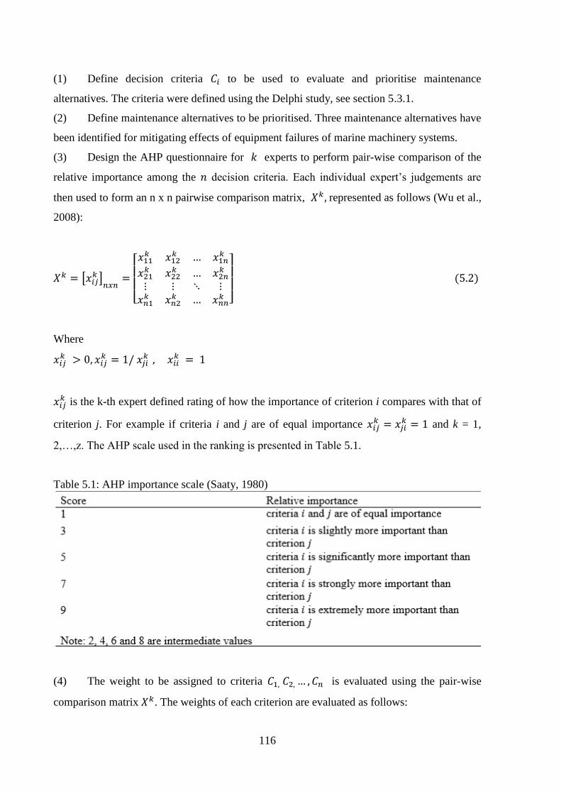
116

(1) Define decision criteria 𝐶𝑖 to be used to evaluate and prioritise maintenance

alternatives. The criteria were defined using the Delphi study, see section 5.3.1.

(2) Define maintenance alternatives to be prioritised. Three maintenance alternatives have

been identified for mitigating effects of equipment failures of marine machinery systems.

(3) Design the AHP questionnaire for 𝑘 experts to perform pair-wise comparison of the

relative importance among the 𝑛 decision criteria. Each individual expert’s judgements are

then used to form an n x n pairwise comparison matrix, 𝑋𝑘 , represented as follows (Wu et al.,

2008):

𝑋𝑘 = [𝑥𝑖𝑗𝑘 ]

𝑛𝑥𝑛=

[ 𝑥11

𝑘 𝑥12𝑘 … 𝑥1𝑛

𝑘

𝑥21𝑘 𝑥22

𝑘 … 𝑥2𝑛𝑘

⋮ ⋮ ⋱ ⋮𝑥𝑛1

𝑘 𝑥𝑛2𝑘 … 𝑥𝑛𝑛

𝑘 ]

(5.2)

Where

𝑥𝑖𝑗𝑘 > 0, 𝑥𝑖𝑗

𝑘 = 1/ 𝑥𝑗𝑖 𝑘 , 𝑥𝑖𝑖

𝑘 = 1

𝑥𝑖𝑗𝑘 is the k-th expert defined rating of how the importance of criterion i compares with that of

criterion j. For example if criteria i and j are of equal importance 𝑥𝑖𝑗𝑘 = 𝑥𝑗𝑖

𝑘 = 1 and k = 1,

2,…,z. The AHP scale used in the ranking is presented in Table 5.1.

Table 5.1: AHP importance scale (Saaty, 1980)

(4) The weight to be assigned to criteria 𝐶1, 𝐶2, … , 𝐶𝑛 is evaluated using the pair-wise

comparison matrix 𝑋𝑘. The weights of each criterion are evaluated as follows:

117

𝑤𝑖𝑘 =

1

𝑛∑

𝑥𝑖𝑗𝑘

∑ 𝑥𝑖𝑗𝑘

𝑖𝑗

(5.3)

Where 𝑤𝑖𝑘 is the weight of criteria 𝐶𝑖

The weights of the criteria can be represented as weight vector (Wk).

𝑾𝒌 = [𝑤1𝑘, 𝑤2

𝑘, … , 𝑤𝑛𝑘]𝑇 (5.4)

(5) The consistency of judgement by the experts is then evaluated using the consistency

ratio 𝐼𝑟, . In general a consistency ratio of less than 0.1 is acceptable and if the value is greater

than this, experts should be advised to revise their initial judgement (Saaty, 1980). The

consistency ratio is calculated as:

𝐼𝑟, = 𝐶𝐼

𝑅𝐼 (5.5)

Where RI is the corresponding average random value of 𝐶𝐼 for an 𝑛 𝑥 𝑛 matrix, the values are

shown in Table 5.2, and 𝐶𝐼 is the consistency index and can be evaluated as

𝐶𝐼 = 𝜆max − 𝑛

𝑛 − 1 (5.6)

Where 𝜆max is the maximum eigenvalue

𝜆max = 1

𝑛∑

(𝑋𝑘𝑤𝑘 )𝑖

𝑤𝑖𝑘

𝑛

𝑖=1

(5.7)

Table 5.2: RI values for different matrix order (Saaty, 1980)

118

(6) The next step is to evaluate the local weight of each maintenance alternative for each

criterion: firstly construct a pairwise comparison matrix between maintenance alternatives for

each criterion using Eq. 5.2 (see the sample given in Table 5.7), next the solution models used

in evaluating criteria pairwise comparison of individual experts i.e. Eq. 5.3 to 5.7 are also

used for the maintenance alternatives’ pairwise comparison matrix to obtain local weight of

each maintenance alternative.

(7) The overall score of each maintenance alternative is evaluated by multiplying the local

weight of a maintenance alternative by criteria local weight and summing over all criteria.

Based on the overall score, maintenance alternatives are ranked and the most appropriate

selected.

(8) Where pairwise comparison judgements are available from more than one expert, the

overall score of each maintenance alternative from individuals is averaged to obtain a group

overall score for the maintenance alternative option (Bolloju, 2001).

The Goepel (2014) AHP online calculator was used for the evaluation of Eq. 5.3-5.7

5.3.3 PROMETHEE method

As discussed in Chapter 4, PROMETHEE is an acronym for Preference Ranking Organisation

METHod for Enrichment Evaluations, a multi-criteria decision making method developed by

Brans, first presented in 1982 (Brans, 1986) and further extended by Brans and Vincke (Brans

and Vincke, 1985). There have been 7 versions developed (Behzadian et al., 2010) and the

one used here is PROMETHEE II. PROMETTHEE II is the most popular of all the versions

and it’s fundamental to the implementation of the other versions. The basic principle of

PROMETHEE II for solving multi-criteria decision problems is the pairwise comparison of

all alternatives for each criterion. The performance of one alternative over another in the

pairwise comparison for each criterion is based on a preference function. This preference

function (PF) turns the difference between two alternatives for each criterion into real values

which range from 0 to 1. This corresponds to the degree of preference a maintenance

practitioner has for one alternative over another. If the difference between two alternatives is

0, it simply means no preference and if the value is 1 its means full preference (Mareschal and

De Smet, 2009). There are six different types of preference function; usual criterion, U-shape

criterion, Gaussian criterion, V-shape criterion V-shape with indifference and level criterion

(Brans et al., 1986). For this study the usual criterion was selected as the preference function

because there is evidence in the literature that it is most suitable for qualitative data

(VPSolution, 2013).

119

Apart from the preference function that needs to be defined by the maintenance practitioners

for the application of PROMETHEE, additional information that needs to be defined are the

weights of the criteria. There are different techniques available for determining the weights of

criteria such as the AHP method, entropy method and variance technique. The AHP technique

was selected for this work as it enables the decision problem to be logically structured, a

feature lacking in the PROMETHEE method. However AHP has the disadvantage of trading

off assigned criteria “good” ratings for “bad” ratings and vice versa because its information

evaluation principle is based on complete aggregation of the additive type which can result in

loss of vital information. In PROMETHEE partial aggregation is used which avoids the trade-

off associated with the complete aggregation technique (Macharis et al., 2004). Additionally,

AHP has a predetermined technique for criteria weight evaluation whereas in the

PROMETHEE technique there is no provision for criteria weight determination thereby

laying an additional burden on the maintenance practitioners. On this basis, a combination of

the two techniques, AHP-PROMETHEE, is proposed for the prioritisation of maintenance

alternatives by utilising the areas of strength of each technique. While AHP is used in the

structuring of the decision problem and weighting of decision criteria, PROMETHEE is

applied in the ranking of the maintenance alternatives.

The basic steps of the PROMETHEE method can be defined as follows:

(1) Definition of the problem: consider a multi-criteria problem of m alternatives (a1,

a2,…,am) and n criteria (c1,c2,…cn).

(2) Determination of deviation based on pairwise comparisons as follows:

𝑑𝑗(𝑎, 𝑏) = 𝑐𝑗 (𝑎) − 𝑐𝑗 (𝑏) (5.8)

Where d is the pairwise difference between evaluations of alternatives a and b for each

criterion

(3) Utilisation of preference function:

𝑃𝑗(𝑎, 𝑏) = 𝐹𝑗{𝑑𝑗(𝑎, 𝑏)} (5.9)

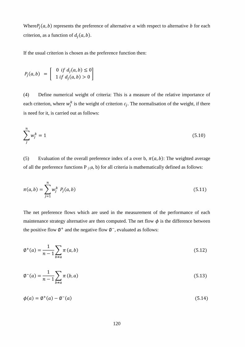
120

Where𝑃𝑗(𝑎, 𝑏) represents the preference of alternative 𝑎 with respect to alternative 𝑏 for each

criterion, as a function of 𝑑𝑗(𝑎, 𝑏).

If the usual criterion is chosen as the preference function then:

𝑃𝑗(𝑎, 𝑏) = [ 0 𝑖𝑓 𝑑𝑗(𝑎, 𝑏) ≤ 0

1 𝑖𝑓 𝑑𝑗(𝑎, 𝑏) > 0 ]

(4) Define numerical weight of criteria: This is a measure of the relative importance of

each criterion, where 𝑤𝑗𝑘 is the weight of criterion 𝑐𝑗. The normalisation of the weight, if there

is need for it, is carried out as follows:

∑𝑤𝑗𝑘

𝑛

𝑗

= 1 (5.10)

(5) Evaluation of the overall preference index of a over b, 𝜋(𝑎, 𝑏): The weighted average

of all the preference functions P j (a, b) for all criteria is mathematically defined as follows:

𝜋(𝑎, 𝑏) = ∑𝑤𝑗𝑘

𝑛

𝑗=1

𝑃𝑗(𝑎, 𝑏) (5.11)

The net preference flows which are used in the measurement of the performance of each

maintenance strategy alternative are then computed. The net flow 𝜙 is the difference between

the positive flow ∅+ and the negative flow ∅−, evaluated as follows:

∅+(𝑎) =1

𝑛 − 1∑ 𝜋

𝑏≠𝑎

(𝑎, 𝑏) (5.12)

∅−(𝑎) =1

𝑛 − 1∑ 𝜋

𝑏≠𝑎

(𝑏, 𝑎) (5.13)

𝜙(𝑎) = ∅+(𝑎) − ∅−(𝑎) (5.14)

121

The maintenance alternatives are ranked on the basis of the net flow and the higher the value

the better the alternative. Having obtained the input information from experts, rather than

manually solving the multi-criteria decision problem by applying Eq. 5.8 to 5.14, Visual

PROMETHEE, developed by Bertrand Mareschal (VPSolution, 2013) was used in processing

the information and in ranking the maintenance alternatives.

5.3.4 TOPSIS method

The TOPSIS methodological steps for choosing an alternative from multiple options have

been previously discussed in Chapter 3 Section 3.3.2.2. Although in Chapter 3 it was applied

in prioritising risk of failure modes of a marine diesel engine, in this current chapter TOPSIS

will be used in the ranking (prioritising) of maintenance strategy alternatives such that the

optimum maintenance strategy will be adopted for the system or component under

investigation.

5.4 Case study of the marine diesel engine

The prioritisation of risk of failure modes of the marine diesel engine had been carried out in

Chapters 3 and 4. From the study, one of the equipment items/components with the greatest

failure consequence on the marine diesel engine was found to be the water cooling pump of

the central cooling system. The water cooling pump was chosen to demonstrate the

applicability of the proposed methodology in the selection of a maintenance strategy.

5.4.1 Delphi evaluation

A panel of ten experts was carefully selected, 5 from academia with 5 to 12 years previous

work experience in the shipping industry and 5 from the shipping industry ranging from 2nd

Engineer to Chief Engineer. A thorough literature survey was conducted on relevant

maintenance strategy selection problems and 22 criteria were initially selected. The 22 criteria

were further subjected to two rounds of Delphi survey in order to critically select the most

relevant evaluation criteria for selection of the maintenance strategy for maritime

applications. The mean of the consensus measurement indices and CVR of all 10 experts’

opinions were evaluated in both first and second round Delphi surveys for each of the

maintenance strategy selection criteria and their corresponding rankings are presented in

Table 5.3 and 5.4. The Delphi iteration process was terminated at the second round because

there was no significant difference between results of the first and second rounds.

122

In Table 5.4, the criteria with the ranking highlighted in pink had mean values below 2.7 and

CVR below 0.29. These criteria were removed and the remaining items retained. Some other

items were further removed because of their overlapping function with other criteria. The

remaining criteria were then re-categorised into main and sub-criteria. For example spare

parts inventories cost, minimisation of loss, maintenance cost, crew training cost and plant

damage are sub criteria under the main criterion cost.

Table 5.3: Result of first round Delphi survey

123

Table 5.4: Result of second round Delphi survey questionnaire

Having defined the decision criteria against which the maintenance strategies will be ranked,

the next step is to apply the ranking tools, AHP, PROMETHEE and TOPSIS in evaluating the

optimum maintenance strategy. Firstly the case studies that are presented use a single expert

information for analysis of the three ranking tools in reaching an optimum solution and then

the use of three experts’ (group decision making) information in reaching an optimum

solution is presented.

124

5.4.2 AHP analysis using information from a single expert

The maintenance strategy selection criteria categorised into main and sub-criteria were used

to form a four level AHP hierarchy decision problem as shown in Figure 5.2. With the first,

second, third and fourth levels representing overall goal (Decision problem), main criteria,

sub-criteria and the alternative maintenance strategy to be selected with respect to the main

and sub criteria, respectively.

To evaluate the problem in figure 5.2, a structured AHP questionnaire was developed and

sent to an expert selected from the Delphi survey team to perform the pairwise comparison

judgement using the Saaty scale in Table 5.1 firstly for the main criteria with respect to the

overall goal, next for the sub-criteria with respect to the main criteria and overall goal and

lastly for the maintenance alternatives with respect to the sub-criteria. The comparison matrix

developed from the expert’s judgement for main criteria is presented in Table 5.5. Samples of

the comparison matrices formed from the expert’s judgement for the sub-criteria and

maintenance alternatives are shown in Tables 5.6 and 5.7. The complete comparison matrices

are presented in Appendix B3.1. It is worth noting that in this research, the consistency of this

expert’s judgement in all scenarios measured using the consistency ratio, 𝐼𝑟 , was in the range

of 0.00 to 0.084 which is within the acceptable value of less than 0.1.

125

Figure 5.2: AHP hierarchy of multi-criteria decision maintenance strategy selection problem

CM-Corrective maintenance, SOH-Scheduled overhaul, SRP-Scheduled replacement,

OFCBM-Offline condition based maintenance, ONCBM-Online condition based maintenance

Next the local weight of the main criteria was evaluated based on Table 5.5 using Eq. 5.3 –

5.7 and the results are presented in Table 5.8. This was followed by applying Eq. 5.3 –5.7 to

Table 5.6 (a sample) to obtain local weight of sub-criteria and the result is shown in Table 5.8.

The global weight of the criteria was generated by aggregating the local weight of the main

criteria and local weight of the sub-criteria and the results are also presented in Table 5.8.

Finally the overall score of the maintenance alternatives was obtained by using steps 6 and 7

of Section 5.4.2 and the results are presented in Table 5.9.

Table 5.5: Main criteria comparison matrix with respect to overall goal

126

Table 5.6: Sub-criteria comparison matrix with respect to main criterion (cost)

Table 5.7: maintenance alternatives comparison matrix with respect to sub-criterion (spare

parts inventories cost)

Table 5.8: Local and aggregated (global) weight of criteria

127

Table 5.9: Maintenance strategies overall score

Comparing the overall scores of the five alternative maintenance strategies in Table 5.9,

offline condition based maintenance (OFCBM) with the highest performance index of 0.3210

was the preferred alternative, followed by online condition based maintenance (ONCBM)

with a weight of 0.3184 and the least preferred was corrective maintenance (CM) with a

priority value of 0.0935. The preferred choice of offline condition based maintenance to

online condition based maintenance is probably due to the fact that it is effective and yet is a

much cheaper means of monitoring the condition of an asset than the online technique. From

this analysis, as it can be seen in Table 5.8, safety criteria have the greatest influence in the

selection of the maintenance strategies for the cooling water pump of a marine diesel engine

with a weight of 54% when compared to other main criteria such as cost, added value and

applicability with weights of 6.9, 19.3 and 19.3% respectively.

5.4.3 TOPSIS and PROMETHEE 2 analysis using a single expert information

For the AHP technique, information was obtained from an expert through a pairwise

comparison method in which alternatives were compared in pairs to ascertain which one is

more important using the Saaty scale for each criterion. However for the other MCDM

techniques such as PROMETHEE and TOPSIS, a 5 point Likert scale was applied in this

study in obtaining information from the expert. In order to have an unbiased comparison of

128

TOPSIS and PROMETHEE with APH that uses the pairwise comparison method, the same

expert was used in obtaining information for the three methods. The values assigned by the

expert for the five maintenance alternatives with respect to 12 decision criteria using a 5 point

Likert scale are shown in Table 5.10.

Table 5.10: Single expert judgement of maintenance alternatives

5.4.3.1 PROMETHEE Analysis using information from a single expert

One of the reasons PROMETHEE is very popular is the availability of software in carrying

out the analysis. In this case the ‘PROMETHEE software’ refers to Visual PROMETHEE

which was used in evaluating information obtained from the expert as given in Table 5.10 and

the criteria weights generated from the AHP analysis in Table 5.8; the purpose being to

determine the optimum maintenance alternative for the water cooling pump.

The decision matrix in Table 5.10 and the decision criteria weights obtained in the AHP

analysis were used to populate the PROMETHEE software to obtained the performance index

based on which the ranking of the five maintenance alternatives; CM, SOH, SRP, OFCBM

and ONCBM was performed. Prior to the PROMETHEE analysis of the data in Table 5.10 a

preference function for each criterion was defined. In this study the ‘usual’ preference

function was chosen for each criterion because it is ideally suited for a qualitative scale with a

low number of levels such as the 5 point Likert scale (VPSolution, 2013). In the usual

preference function, actual values are not important in determining preference of one

alternative to another and what is important is the order: best to worst. This characteristic

actually makes it ideal for ordinal scale data in contrast to the other preference functions that

129

turn the difference between two alternatives into a real value i.e. from 0 and 1 (De Keyser and

Peeters, 1996). After defining the preference function for each criterion, the performance

index net flow which is the difference between the positive flow and the negative flow is then

evaluated with Visual PROMETHEE. The results of the net flow, 𝜙, together with the

positive flow, ∅+, and negative flow, ∅−, for the five maintenance alternatives are presented

in Table 5.11.

Table 5.11: PROMETHEE flow

The alternative with the highest value of net flow 𝜙 is considered to be the best alternative

while the alternative with the lowest value of net flow is the worst solution. From Table 5.11,

OFCBM with the highest value of net flow is the best alternative, followed by ONCBM and

the worst alternative is CM. The values of net flow obtained in this case were based on the

selection of the preference function referred to as ‘usual criterion’, these values would not be

the same if other preference functions were selected for the evaluation. Therefore obtaining a

reliable and efficient result using the PROMETHEE technique depends greatly on the

maintenance practitioner’s ability to identify the appropriate preference function for each

criterion. This creates an additional burden on the maintenance practitioner. Another factor

that greatly impacts on the ranking is the weight of the criteria.

Sensitivity Analysis:

In order to test the robustness of the technique, a sensitivity analysis was carried out by

changing the weight of different criteria to see the resulting effect with respect to the ranking

order of the five maintenance alternatives. The results which are shown in Table 5.12 reveal

the lower and upper limit a decision criterion weight can vary between without changing the

order of ranking of the five maintenance alternatives. From the result it can be seen that the

changes in weight of criteria C2, C3, S2, A1, A2 and A3 beyond 40.75%, 17.44%, 31.88%,

28.52% 47.77% and 22.42% respectively will lead to alteration in the ranking of the five

maintenance alternatives while for the other criteria, changes in their weights will not lead to

130

changes in the ranking order. In essence criteria C3 has the greatest impact on the ranking

followed by A3. This sensitivity analysis has demonstrated the robustness of the

PROMETHEE technique in the prioritisation of the maintenance strategy alternatives.

Table 5.12: Stability interval

5.4.3.2 TOPSIS Analysis using single expert information

In the application of TOPSIS to the water cooling pump of a marine diesel engine, the

decision matrix in Table 5.10 was normalised using Eq. (3.6) and the result is presented in

Table 5.13. The normalised matrix was then multiplied by the criteria weights in Table 5.8 to

obtain a weighted normalised matrix also shown in Table 5.13. Eq. (3.10) and (3.11) were

then utilised to determine the positive ideal and negative ideal solutions respectively as

presented in Table 5.14. Finally, applying Eq. (3.12) – (3.14) the distance of each

maintenance strategy alternative to the positive-ideal solution 𝐷𝑖+ and to the negative-ideal

solution 𝐷𝑖− together with relative closeness 𝑅𝐶𝑖 of each failure mode to the ideal solution

were calculated and the results of 𝑅𝐶𝑖 together with their rankings are shown in Table 5.15.

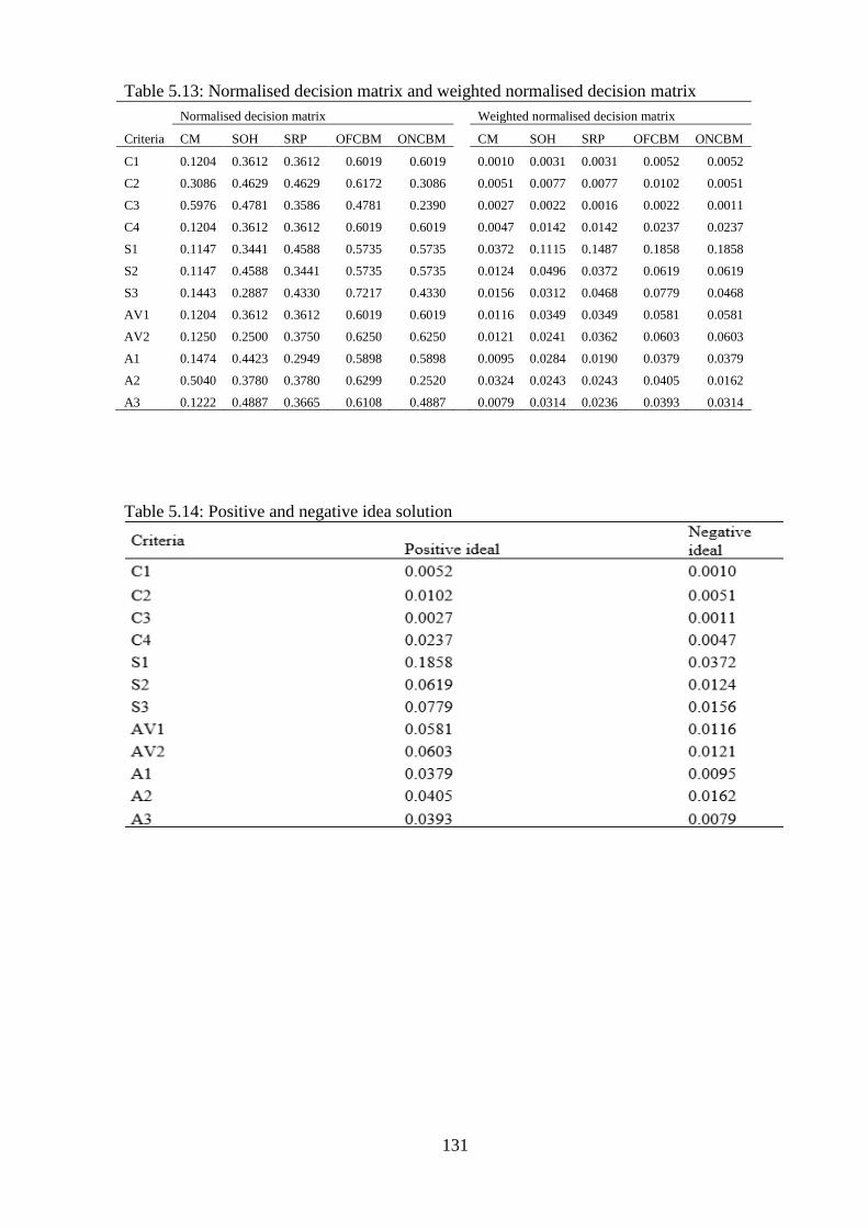
131

Table 5.13: Normalised decision matrix and weighted normalised decision matrix

Criteria

Normalised decision matrix

Weighted normalised decision matrix

CM SOH SRP OFCBM ONCBM

CM SOH SRP OFCBM ONCBM

C1 0.1204 0.3612 0.3612 0.6019 0.6019

0.0010 0.0031 0.0031 0.0052 0.0052

C2 0.3086 0.4629 0.4629 0.6172 0.3086

0.0051 0.0077 0.0077 0.0102 0.0051

C3 0.5976 0.4781 0.3586 0.4781 0.2390

0.0027 0.0022 0.0016 0.0022 0.0011

C4 0.1204 0.3612 0.3612 0.6019 0.6019

0.0047 0.0142 0.0142 0.0237 0.0237

S1 0.1147 0.3441 0.4588 0.5735 0.5735

0.0372 0.1115 0.1487 0.1858 0.1858

S2 0.1147 0.4588 0.3441 0.5735 0.5735

0.0124 0.0496 0.0372 0.0619 0.0619

S3 0.1443 0.2887 0.4330 0.7217 0.4330

0.0156 0.0312 0.0468 0.0779 0.0468

AV1 0.1204 0.3612 0.3612 0.6019 0.6019

0.0116 0.0349 0.0349 0.0581 0.0581

AV2 0.1250 0.2500 0.3750 0.6250 0.6250

0.0121 0.0241 0.0362 0.0603 0.0603

A1 0.1474 0.4423 0.2949 0.5898 0.5898

0.0095 0.0284 0.0190 0.0379 0.0379

A2 0.5040 0.3780 0.3780 0.6299 0.2520

0.0324 0.0243 0.0243 0.0405 0.0162

A3 0.1222 0.4887 0.3665 0.6108 0.4887

0.0079 0.0314 0.0236 0.0393 0.0314

Table 5.14: Positive and negative idea solution

132

Table 5.15: Performance index (RC) and rank

From Table 5.15 it is obvious that the optimum maintenance alternative is the OFCBM since

it occupies the first position and it has performance index of 0.9972 which is closest to the

ideal solution. This is followed by ONCBM and the least preferred maintenance strategy is

CM having the lowest performance index of 0.1357 and being in the fifth position.

5.4.4 Comparison of methods

The comparison of the rankings obtained from the three MCDM methods are presented in

Table 5.16. From the table, OFCBM appears in first position for all the ranking models and as

such is the optimum solution for all of the techniques. Also from the table, last position is

occupied by CM for the three ranking models; AHP, PROMETHEE and TOPSIS. The

Spearman rank correlation coefficients between the three MCDM techniques are presented in

table 5.17.

Table 5.16: Comparison of rankings from methods

133

Table 5.17: Spearman’s rank correlation between methods

From Table 5.17 the Spearman rank correlation coefficient between PROMETHEE and

TOPSIS is 1, between AHP and PROMETHEE is 0.937 and between PROMETHEE and

TOPSIS is 0.937. The perfect and near perfect correlation between the three methods shows

that the three techniques can be used singly or in combination with one another for the

purpose of prioritising maintenance strategy alternatives. This has also validated the

applicability of the different MCDM techniques proposed for the selection of the maintenance

strategy for the components of marine machinery systems from numerous alternatives.

5.4.5 Group decision making

The case considered above is a situation whereby a single expert is involved in the decision

making process. However in many practical situations multiple experts or a group of experts

are involved in the decision making process thereby bringing a great deal of complexity into

the use of MCDM methods (Raju et al., 2000). Different aggregation methods are available

for combining experts’ preferences in group decision making. Either rank or score

aggregation can be used. In this research the score aggregation technique was chosen because

rank aggregation may lead to rank reversal. In aggregating the scores of individual experts a

simple arithmetic mean can be applied. The average of the individual experts AHP scores,

PROMETHEE and TOPSIS scores for each maintenance alternative are referred to here as

group scores. On the basis of the group score, maintenance strategy alternatives were ranked

and the highest ranked chosen as the optimum solution.

As previously stated, for AHP the input information is obtained from experts’ comparison

judgement which is then used in forming comparison matrices. Three of the original ten

experts used for the Delphi analysis were used in this group decision making process, the

scores obtained for the single expert case studied above will be referred to as expert 1 scores

while the expert 2 and 3 scores for the five alternative maintenance strategies were

134

determined based on comparison judgement obtained from experts 2 and 3. The comparison

judgements obtained from experts 2 and 3 are presented in Appendix B3.2 and B3.3

respectively.

However PROMETHEE and TOPSIS, require the use of an ordinal scale in the rating of

maintenance alternatives against decision criteria. The rating was carried out by the same

experts that performed the comparison judgement to ensure unbiased comparison between

AHP, TOPSIS and PROMETHEE. The rating obtained from expert 1 was presented in Table

5.10 while the ratings obtained from experts 2 and 3 are presented in Table 5.18. Since AHP,

TOPSIS and PROMETHEE had already been applied to the data from expert 1 in Sections

5.4.2 and 5.4.3, only evaluation for experts 2 and 3 will be shown subsequently.

Table 5.18: Experts 2 and 3 judgement of five maintenance alternative

5.4.5.1 Evaluation of AHP group maintenance strategy alternatives

AHP analysis using expert 2 comparison judgement

The pairwise comparison judgements obtained from expert 2 were firstly used in producing

decision matrices which are presented in Appendix B3.2. The comparison matrices were then

subjected to AHP analysis to obtain the weightings of the main criteria together with the

weightings of sub-criteria and the global weight of sub-criteria. The results are presented in

Table 5.19. Finally, overall alternative maintenance strategy scores were obtained as a

135

product of the global weight of sub-criteria and the weight of maintenance alternatives with

respect to the decision criteria and the results are shown in Table 5.20.

Table 5.19: Local and aggregated (global) weight of criteria for expert 2

Table 5.20: Maintenance strategies overall score

136

AHP analysis using expert 3 comparison judgement

Having obtained maintenance alternatives’ overall scores from experts’ 1 and 2 pairwise

comparison judgement, the same AHP procedure was followed in evaluating the overall

maintenance alternative scores for expert 3. Firstly the pairwise comparison judgements

obtained from expert 3 were converted to comparison matrices which are presented in

Appendix B3.3. Applying AHP evaluation techniques to the expert 3 pairwise comparison

matrices, the weight of the main criteria together with weight of sub-criteria, the global

weight of sub-criteria were evaluated and overall maintenance alternative scores obtained.

The results of the weight of the main criteria together with weight of sub-criteria and the

global weight of sub-criteria are presented in Table 5.21 while the results of the of the overall

maintenance alternative scores are presented in Table 5.22.

Table 5.21: Local and aggregated (global) weight of criteria for expert 3

137

Table 5.22: Maintenance strategies overall score

As previously stated, to obtain the group overall rating of maintenance strategy alternatives

the individual experts ratings were averaged, as shown in Table 5.23. From the result, it is

again obvious that the preferred maintenance strategy alternative is OFCBM, having the

highest group overall score of 0.3335. This is followed by ONCBM and the least preferred

option is CM having the lowest group overall score of 0.0835. There is no difference between

the group rating and the individual expert rating since the same ranking order was obtained.

This is as a result of the similarity in the comparison judgement of the five maintenance

alternatives against decision criteria obtained from the three experts.

Table 5.23: Group decision making AHP score and ranks

138

5.4.5.2 Evaluation of the PROMETHEE group maintenance strategy alternatives

The decision matrix formed from expert 1’s rating of maintenance strategies against decision

criteria was firstly subjected to PROMETHEE analysis to obtain the expert 1 PROMETHEE

overall score for the maintenance alternatives upon which the maintenance alternatives were

ranked. This was carried out in section 5.4.3.1. This was then followed by subjecting data

from experts 2 and 3 to PROMETHEE analysis to obtain expert 2 and 3 overall scores (𝜙

values) of maintenance strategy alternatives. To obtain the group overall scores for

maintenance alternatives, the individual experts’ scores were averaged.

PROMETHEE analysis using expert 2 judgement

The expert 2 decision matrix in Table 5.18 and the criteria weights evaluated from the expert

2 AHP analysis of comparison judgement in Table 5.19 were used as input data for the

PROMETHEE software to obtain overall scores (𝜙 values) of maintenance strategy

alternatives. The maintenance strategy alternatives were ranked based on the 𝜙 values.

As with the analysis for expert 1, the preference function was the “usual” type. The overall

scores of maintenance alternatives were then determined using the PROMETHEE software

and the result obtained is displayed in Table 5.24.

Table 5.24: PROMETHEE flow for expert 2

From Table 5.24, the offline condition based maintenance (ONCBM) with the highest value

of net flow, 𝜙, was the best ranked maintenance alternative while the worst rank was

corrective maintenance CM.

Sensitivity Analysis:

A sensitivity analysis was again carried out to test the robustness of the PROMETHEE

technique. The results are presented in Table 5.25. From the table, changes in criteria weights

139

C2, C3, C4, AV1, A1 and A2 beyond a certain level (17.93%, 28.29%, 40.75%, 47.24%,

29.08 and 20.01% respectively) resulted in changes in the ranking order of the five

maintenance alternatives. For the other criteria irrespective of the changes in the weights of

the criteria, the ranking order remained unchanged. It is obvious that the criteria that cause

alteration in the order of ranking have the greatest influence on the ranking of maintenance

alternatives.

Table 5.25: Stability intervals for expert 2

PROMETHEE analysis using expert 3 judgement

The expert 3 decision matrix in Table 5.18 and the criteria weights evaluated from the expert

3 AHP analysis of comparison judgements in Table 5.21 were used as input data in the

PROMETHEE analysis to obtained overall scores (𝜙 values) of maintenance strategy

alternatives and the maintenance strategy alternatives were ranked based on the 𝜙 values.

The preference function type 1 was again chosen as in the cases of experts 1 and 2. The

overall scores (𝜙 values) of the maintenance strategy alternatives were then determined and

the five maintenance strategy alternatives ranked. The results obtained are shown in Table

5.26.

140

Table 5.26: PROMETHEE flow for expert 3

Sensitivity Analysis:

A sensitivity analysis was again carried out and the results are presented in Table 5.27.

Table 5.27: Stability interval for expert 3

From the results in Table 5.27, if criteria C2, C3, S3, A1 and A2 weights are increased by up

to 29.55%, 15.61%, 20.16%, 34.70%, and 29.17% respectively, the order of ranking of

maintenance alternatives in Table 5.26 will remain unchanged. However if these limits are

exceeded the ranking order will be altered while for the other criteria, irrespective of the

weight increase, the ranking order will remain unaltered.

To obtain the group overall scores of maintenance strategy alternatives, the individual experts

overall scores were averaged, as shown in Table 5.28. From the result it is again obvious that

the preferred maintenance strategy alternative is OFCBM, having the highest group overall

141

score of 0.7681. This is followed by ONCBM and the least preferred choice is CM having the

lowest group overall score of -0.7972.

Table 5.28: Multiple experts decision making score and rank

5.4.5.3 Evaluation of the TOPSIS group maintenance strategy alternatives

TOPSIS was also applied to the maintenance strategy selection using data from the three

experts. The expert 1 overall scores (RCi values) for each of the maintenance strategy

alternatives were evaluated in Section 5.4.3.2. The expert 2 and 3 overall scores for each of

the maintenance strategy alternatives are evaluated next. The average of the three experts

maintenance strategy alternatives scores were then used to obtain the group overall scores of

maintenance strategy alternatives.

TOPSIS Analysis using expert 2 judgement

TOPSIS analysis was applied to the expert 2 decision matrix given in Table 5.18. The expert

2 decision matrix in Table 5.18 was first normalised using Eq. (3.6) and then multiplied by

the criteria weights in Table 5.19 to obtain a weighted normalised matrix. Both the normalised

decision matrix and the weighted normalised decision matrix are shown in Table 5.29. Eq.

(3.10) and (3.11) were then utilised to determine the positive ideal and negative ideal

solutions respectively as presented in Table 5.30. Finally, applying Eq. (3.12) – (3.14), the

distance of each maintenance strategy alternative to the positive-ideal solution 𝐷𝑖+ and the

negative-ideal solution 𝐷𝑖− together with relative closeness 𝑅𝐶𝑖 of alternative maintenance

strategy to the ideal solution were calculated and the results are shown in Table 5.31. Based

on the relative closeness 𝑅𝐶𝑖 of each alternative maintenance strategy to the ideal solution, the

maintenance strategy alternatives were ranked as also shown in Table 5.31.

142

Table 5.29: Expert 2 normalised decision matrix and weighted normalised decision matrix

Criteria

Normalised decision matrix

Weighted normalised decision matrix

CM SOH SRP OFCBM ONCBM

CM SOH SRP OFCBM ONCBM

C1 0.2857 0.4286 0.2857 0.5714 0.5714

0.0020 0.0030 0.0020 0.0041 0.0041

C2 0.5774 0.4619 0.3464 0.4619 0.3464

0.0270 0.0216 0.0162 0.0216 0.0162

C3 0.4619 0.3464 0.4619 0.5774 0.3464

0.0216 0.0162 0.0216 0.0270 0.0162

C4 0.1187 0.2374 0.4747 0.5934 0.5934

0.0021 0.0041 0.0082 0.0103 0.0103

S1 0.1250 0.3750 0.2500 0.6250 0.6250

0.0365 0.1096 0.0731 0.1826 0.1826

S2 0.1204 0.3612 0.3612 0.6019 0.6019

0.0117 0.0352 0.0352 0.0586 0.0586

S3 0.2357 0.3536 0.3536 0.5893 0.5893

0.0230 0.0344 0.0344 0.0574 0.0574

AV1 0.2520 0.3780 0.3780 0.5040 0.6299

0.0348 0.0522 0.0522 0.0695 0.0869

AV2 0.2390 0.4781 0.3586 0.5976 0.4781

0.0330 0.0660 0.0495 0.0825 0.0660

A1 0.3939 0.5252 0.2626 0.6565 0.2626

0.0093 0.0124 0.0062 0.0155 0.0062

A2 0.6934 0.4160 0.1387 0.5547 0.1387

0.0491 0.0295 0.0098 0.0393 0.0098

A3 0.2673 0.4009 0.4009 0.6682 0.4009

0.0063 0.0095 0.0095 0.0158 0.0095

Table 5.30: Expert 2 negative and positive ideal solution

143

Table 5.31: Performance index and Rank

TOPSIS Analysis using expert 3 judgement

The expert 3 matrix in Table 5.18 was normalised using Eq. (3.6) and then multiplied by the

criteria weights given in Table 5.21 to obtain a weighted normalised matrix. The normalised

decision matrix and the weighted normalised decision matrix determined are presented in

Table 5.32. To obtain the positive ideal and negative ideal solution in Table 5.33 Eq. (3.10)

and (3.11) were applied to the weighted normalised matrix. Finally applying Eq. (3.12) –

(3.14), the distance of each maintenance strategy alternative to the positive-ideal solution

𝐷𝑖+ and to the negative-ideal solution 𝐷𝑖

− together with relative closeness 𝑅𝐶𝑖 to the ideal

solution were evaluated and the results together with the corresponding rankings are shown in

Table 5.34.

Table 5.32: Expert 3 normalised decision matrix and weighted normalised decision matrix

Criteria

Normalised decision matrix

Weighted normalised decision matrix

CM SOH SRP OFCBM ONCBM

CM SOH SRP OFCBM ONCBM

C1 0.1459 0.2917 0.1459 0.7293 0.5835

0.0033 0.0067 0.0033 0.0166 0.0133

C2 0.3050 0.3050 0.1525 0.7625 0.4575

0.0023 0.0023 0.0011 0.0057 0.0034

C3 0.7906 0.4743 0.1581 0.3162 0.1581

0.0066 0.0039 0.0013 0.0026 0.0013

C4 0.1098 0.4391 0.4391 0.5488 0.5488

0.0003 0.0011 0.0011 0.0013 0.0013

S1 0.1147 0.4588 0.3441 0.5735 0.5735

0.0529 0.2118 0.1588 0.2647 0.2647

S2 0.1147 0.4588 0.3441 0.5735 0.5735

0.0100 0.0402 0.0301 0.0502 0.0502

S3 0.6868 0.2747 0.2747 0.5494 0.2747

0.0266 0.0107 0.0107 0.0213 0.0107

AV1 0.1187 0.4747 0.2374 0.5934 0.5934

0.0042 0.0169 0.0084 0.0211 0.0211

AV2 0.1187 0.4747 0.2374 0.5934 0.5934

0.0042 0.0169 0.0084 0.0211 0.0211

A1 0.1400 0.4201 0.5601 0.5601 0.4201

0.0038 0.0115 0.0153 0.0153 0.0115

A2 0.4121 0.4121 0.1374 0.6868 0.4121

0.0310 0.0310 0.0103 0.0517 0.0310

A3 0.1250 0.3750 0.2500 0.6250 0.6250

0.0259 0.0778 0.0519 0.1296 0.1296

144

Table 5.33: Negative and positive idea values

Table 5.34: Performance index and ranks

The group overall scores of maintenance strategy alternatives were evaluated by averaging the

individual experts overall scores and the result is shown in Table 5.35. From the table,

OFCBM occupies the first position having a group overall score of 0.9542. Hence the

preferred maintenance strategy alternative is OFCBM. This is followed by ONCBM and the

least preferred choice is CM with the lowest group overall score of 0.1639.

145

Table 5.35: multiple experts’ decision making score and rank

5.4.5.4 Comparison of the proposed hybrid MCDM technique group ranking

The comparison of group ranking of maintenance strategy alternatives obtained from the three

MCDM methods is presented in Table 5.36. From the table, OFCBM appears in first position

for all of the ranking models and as such is the optimum solution is the OFCBM. Also from

the table, last position is occupied by CM for the three ranking models; AHP, PROMETHEE

and TOPSIS. The Spearman rank correlation was also used to determine the relationship

between group rankings obtained from the three methods and the results are presented in

Table 5.37.

Table 5.36: Comparison of group ranking from methods

Table 5.37: Spear man’s rank correlation between methods

146

5.5 Summary

In this chapter, three hybrid MCDM techniques; (1) Delphi-AHP and (2) Delphi-AHP-

PROMETHEE and (3) Delphi-AHP-TOPSIS have been presented for the selection of a

maintenance strategy for marine machinery systems. In the three proposed hybrid MCDM

techniques, Delphi was applied to reduce the number of criteria such that only the most

significant criteria were used in the maintenance alternative decision problem. The aim was to

make the evaluation process as simple as possible such that it could easily be adopted by

shipping system maintenance practitioners. AHP, which has the capability of incorporating

quantitative and qualitative information, was used in the first proposed MCDM technique

(Delphi-AHP) as a tool for determining the decision criteria weight and for the final ranking

of the maintenance strategy alternatives with respect to decision criteria. In the second

proposed MCDM technique (Delphi-AHP-PROMETHEE) AHP was applied as a tool for

evaluating weights of decision criteria while PROMETHEE was used in the ranking of the

maintenance strategy alternatives. In the third proposed MCDM technique (Delphi-AHP-

TOPSIS) AHP was used for the weighting of decision criteria while TOPSIS was applied for

the prioritisation of the maintenance strategy alternatives. The three hybrid methods were

used in addressing a maintenance strategy selection problem involving a single expert firstly

in the decision making process and this was followed by involving three experts (group) in

the decision making process. For both the single expert and group decision making process

the Spearman rank correlation between the three hybrid MCDM techniques was very strong

and, as such a conclusion can be drawn that the three MCDM hybrid techniques can be used

individually or in combination with one another in selecting the maintenance strategy for a

marine machinery system or other related engineering system. Also from the analysis, there

was no significant difference between the group rating and the single expert rating as a result

of the similarity in the judgement of the five maintenance alternatives against decision criteria

obtained from the three experts otherwise the ranking order would have altered significantly.

Another reason is that since only five maintenance strategy alternatives were available, the

degree of freedom was limited. If more alternatives were available there would be more

chance of alteration in the ranking order of maintenance alternatives. Furthermore, from the

analysis, the driving force for the selection of maintenance alternatives for critical marine

machinery equipment is safety which was assigned half of the total weight of decision criteria.

147

For the two scenarios, single expert and group decision making, the selected maintenance

alternative for the water cooling pump of the marine diesel engine was offline condition based

maintenance (OFCBM). This is in line with current best practice. The proposed MCDM

methodologies are simple and yet robust and effectively incorporate the RCM methodology

decision criteria of cost and applicability in addition to other important decision criteria such

as safety and added value which are not usually part of the RCM. Although AHP,

PROMETHEE and TOPSIS produced almost completely the same ranking result for the five

maintenance strategy alternatives for the single expert and group decision making process,

PROMETHEE and TOPSIS would be recommended for those maintenance practitioners who

may find generating numerous pairwise comparison judgments too laborious compared to the

use of a Likert scale that can be applied in generating data for PROMETHEE and TOPSIS

analysis.

Although the proposed methods have been validated for marine machinery systems they can

also be applied to other related engineering systems and, depending on the preference of the

maintenance practitioners, the decision criteria can further be reduced to make the evaluation

process easier.

148

Chapter 6 Scheduled Replacement Interval Determination

6.1 Introduction

The task of determining the maintenance strategy was performed in Chapter 5. Marine

machinery systems are made up of many components/equipment items that require different

maintenance approaches. Hence there is a need to define the optimum maintenance strategy

for each of the critical components/equipment items. After the determination of the of the

appropriate maintenance strategy for each component of the system the next task is to

determine the optimum interval for performing the maintenance task. This is the third stage of

the Reliability Centered Maintenance approach in the optimisation of maintenance (Rausand

and Vatn, 1998).

As stated in the literature review, there are three major maintenance strategies in the RCM

methodology for eliminating or mitigating failure of machinery equipment; corrective

maintenance, Preventive maintenance and condition based maintenance. Time based

preventive maintenance can further be divided into scheduled overhaul and scheduled

replacement while condition based maintenance is sub-divided into on-line condition based

maintenance and off-line condition based maintenance. This chapter presents a technique for

determining the optimal maintenance interval for scheduled replacement while the technique

for determining the optimum interval for off-line condition based maintenance (inspection) is

presented in Chapter 7.

The chapter is organised as follows: in Section 6.2 the proposed scheduled replacement

interval determination methodology is presented. In Section 6.3 the case of the marine diesel

engine cooling water pump is presented. Finally conclusions are presented in Section 6.4.

6.2 Proposed scheduled replacement interval determination methodology

In this research, after analysis of the literature in Chapter 2, a need was identified to introduce

a multi-criteria decision making (MCDM) methodology as a decision support tool in

determining the optimum interval for carrying out scheduled replacement tasks for marine

149

machinery systems. The basis was the following few land-based applications found literature;

(Cavalcante et al., 2010, Cavalcante and De Almeida, 2007, Chareonsuk et al., 1997).

However the proposed MCDM approach for marine system maintenance is intended to be

devoid of the limitations of the approaches used for land-based systems in the literature. To

achieve this objective, firstly a multi-criteria decision making approach based on systematic

application of TOPSIS was applied for marine systems as opposed to the PROMETHEE

technique used for land based applications. Secondly, since the key factors that influence the

selection of intervals are the decision criteria, an efficient framework which integrates

subjective and objective criteria weighting techniques is introduced for evaluating weights of

criteria as opposed to the use of only subjective techniques identified for land based system

applications in the literature. The weighting framework is flexible and it allows maintenance

practitioners to either use subjective criteria weighting techniques or objective weighting

techniques or a combination of the two.

The first step in this methodology is the identification of possible scheduled replacement

intervals for implementing maintenance replacement activities. The experience of the

maintenance team is vital with respect to determining feasible scheduled replacement

intervals. In addition, the manufacturer’s manual for an equipment item can also be of help.

The optimum interval is then selected based on preferred criteria. The criteria that may be

considered are cost, reliability, availability, maintainability, spare parts inventory, quality

issues and maintenance downtime (Chareonsuk et al., 1997). In this research, maintenance

cost, reliability and maintenance downtime were considered. The maintenance cost criterion

was chosen because it constitutes a major portion of the operating cost of ship systems. As

previously stated, for a shipping company to remain in business in a deregulated and

competitive environment, the cost of operation must be optimised and one way to achieved

this is to minimise the cost of ship system maintenance. However in minimising cost,

adequate care must be taken not to compromise the reliability of the system. This is because if

the reliability of the system is compromised, it can result in catastrophic failure that may have

irreversible damage on personnel, equipment and the environment. This makes reliability an

important criterion that must not be ignored in selecting the optimum replacement interval for

ship machinery systems. The downtime criterion was also chosen because downtime of

equipment can produce detrimental penalties. For example, for a ship carrying perishable

goods, the goods can be spoilt and this can result in the ship operator compensating the

owners of the goods. Furthermore the image of the company can also be badly damaged.

150

Data availability is central to the successful selection of the optimum interval for scheduled

replacement activities and as such data should be collected for the system being investigated.

However for equipment which deteriorates with time such as marine machinery systems a

Weibull distribution is generally applicable to fit the collected failure data (O'Connor, 1985).

On this basis, the Weibull distribution function is assumed in this study. The Weibull

distribution was applied to the component life data in evaluating the scale parameter ∅, shape

parameter β and location parameter γ. This was followed by calculation of the criteria values

using criteria models for the different alternative intervals. The decision criteria were

modelled in this research using the Age Replacement Model (ARM). Another possible

technique that can be used in modelling the decision criteria is the Block Replacement Model

(BRM) (Wang, 2002). However ARM has been chosen as the tool for modelling the decision

criteria because the BRM, in most scenarios, results in unnecessary replacement of

equipment/components which makes the ARM technique more cost effective (Ahmad et al.,

2011b). Criteria weights were then evaluated and finally a multi-criteria decision tool based

on TOPSIS was used to aggregate values of criteria with the weights of criteria in order to

determine the optimum preventive interval. The flowchart of this methodology is shown in

Figure 6.1.

151

Figure 6.1: Flowchart of methodology

6.2.1 Weibull distribution

The Weibull distribution is one of the most popular probability distributions for modelling

the failure behaviour of practical systems, especially equipment that deteriorates with time

(Ebeling, 2004). The hazard function rate of the distribution is not constant with time unlike

the exponential distribution (Ebeling, 2004). The Weibull distribution comes in different

forms; one, two and three parameters versions. The key advantage of this type of distribution

is its versatility as it may be applicable in modelling systems or components with increasing

or decreasing failure rates. However its use is limited by availability of adequate data for

152

defining the Weibull parameters and this data may be very difficult to access, especially in the

marine industry. The three parameter Weibull distribution probability density function is

represented as:

𝑓(𝑡) =𝛽

∅[(

𝑡 − 𝛾

∅)]

𝛽−1

exp −(𝑡 − 𝛾

∅)𝛽

(6.1)

Where t ≥ 0, ∅, β and γ > 0

β is the shape parameter which expresses the form of the distribution, 𝛾 is the location

parameter which describe the location of the distribution and ∅ is the scale parameter which

influences the spread of the distribution.

While the cumulative density function is:

𝐹(𝑡) = 1 − 𝑒𝑥𝑝 [−(𝑡 − 𝛾

∅)𝛽

] (6.2)

For the two parameter Weibull the probability density function is as follows:

𝑓(𝑡) =𝛽

∅(𝑡

∅)𝛽−1

𝑒𝑥𝑝 [−(𝑡

∅)𝛽

] (6.3)

Where t ≥ 0, ∅ > 0 and β > 0

While the cumulative density function is as follows:

𝐹(𝑡) = 1 − 𝑒𝑥𝑝 [−(𝑡

∅)

𝛽

] (6.4)

6.2.1.1 Data types

Failure data is generally classified as: complete data or censored data.

Complete data: Failure data is said to be complete when time of failure of all units

investigated are known. For example if failure data of a marine diesel engine is collected for a

153

period of say 5 years and within the period, time to failure of all the components are known

and recorded.

Censored data: Censoring occurs when the exact time to failure of an item is unknown and

either failure occurred before the assumed time or after. Censored data is further categorised

into three groups; right censored data, interval censored data and left censored data. Right

censored data arises when there is doubt about the exact times of failure of some units but it is

known that it happened after some specified time. Left censored data arises when there is

doubt about the exact times of failure of some units but it is known to have happened before

some specified times. Interval censored data is when there is doubt as to the precise times of

failure of some units within an interval.

6.2.1.2 Parameter estimation

Several techniques such as probability plotting, regression analysis, method of moment and

maximum likelihood estimation have been developed for determining parameters ∅, β and γ

that will fit a distribution to a particular data set. The choice of method is a dependent on the

data type collected and in some scenarios the type of distribution selected. When a complete

set of data for machinery is available, regression analysis is generally more appropriate.

However in most real life situations that may not be realistic as data is subjected to censoring.

The maximum likelihood technique is usually the most suitable for analysing a data set with a

relatively large amount of censoring (Cohen, 1965).

Maximum likelihood estimation

The maximum likelihood estimation technique can be used to obtain parameters for any life

distribution such as a Weibull distribution that will best describe the given failure data. The

beauty of this technique is that it is capable of handling problems with varying degrees of

censored data.

Considering T as a continuous random variable with probability density function

𝑓(𝑡𝑖, 𝜃1,𝜃2, … , 𝜃𝑘 ), where 𝜃 are the parameters of the distribution which are candidates for

evaluation and 𝑡1,𝑡2, … , 𝑡𝑛 are failure time data collected for the machinery system. The

likelihood function is determined as follows (Al-Fawzan, 2000, Cohen, 1965):

154

𝐿 = ∏𝑓

𝑛

𝑖=1

(𝑡𝑖; 𝜃1,𝜃2, … , 𝜃𝑘 ) (6.5)

L or the natural logarithm of it is then partially differentiated with respect to 𝜃1,𝜃2, … , 𝜃𝑘

which will then result in equations for obtaining the estimated values of 𝜃1,𝜃2, … , 𝜃𝑘 . The

partial derivative of natural log of L is as follows:

𝜕 ln 𝐿

𝜕𝜃𝑗 = 0 𝑗 = 1,2, … , 𝑘. (6.6)

This technique may be illustrated through application to the probability density function of a 2

parameter Weilbull distribution function given in Eq. (6.3) to estimate the Weibull

parameters; ∅ and β as presented in the work of (Al-Fawzan, 2000, Cohen, 1965). This is as

follows:

𝐿(𝑡1,𝑡2, … , 𝑡𝑘 ; 𝛽, ∅ ) = ∏𝛽

∅(𝑡𝑖∅)𝛽−1

𝑛

𝑖=1

𝑒𝑥𝑝 [− (𝑡𝑖∅)𝛽

] (6.7)

The logarithm of Eq. (6.7) was taken and partially differentiated with respect to ϕ and β

respectively and equated to zero which resulted in Eq. (6.8) and (6.9).

𝜕 ln 𝐿

𝜕β= −

∅

𝛽+ ∑ln 𝑡𝑖

𝑛

𝑖=1

−1

∅∑𝑡𝑖

𝛽ln 𝑡𝑖

𝑛

𝑖=1

= 0 (6.8)

𝜕 ln 𝐿

𝜕∅=

𝑛

∅+

1

∅2∑𝑡𝑖

𝛽

𝑛

𝑖=1

= 0 (6.9)

Equation (6.8) and (6.9) were reduced to:

∑ 𝑡𝑖𝛽ln 𝑡𝑖

𝑛𝑖=1

∑ 𝑡𝑖𝛽𝑛

𝑖=1

−1

𝛽−

1

𝑛∑ln 𝑡𝑖

𝑛

𝑖=1

= 0 (6.10)

155

From here the first step is to evaluate 𝛽 using a standard iterative procedure such as the

Newton-Raphson method. Finally ∅ may be determined using Eq. (6.10) which produces

∅ = √∑ 𝑡𝑖

𝑛𝑖=1

𝑛

𝛽

(6.11)

6.2.2 Criteria function

The scheduled replacement interval selection decision making is based on decision criteria

generally defined by the maintenance managers. In this study as previously stated, cost,

reliability and maintenance down time are the criteria upon which the optimum interval will

be selected. Two factors that influence the selection process are the weights and values of the

criteria. In assigning values to criteria, experts’ opinion is relied on in the face of a lack of or

limited reliable failure data and that approach is qualitative. However the concern here is the

quantitative approach that relies heavily on data availability. Quantitative mathematical

functions are used in evaluating values of decision criteria (reliability, cost and down time)

which are illustrated as follows.

Reliability function: The probability that a system will survive to a particular time t, is

referred to as reliability (Jardine and Tsang, 2013). The Reliability function is thus

represented as follows:

𝑅(𝑡𝑝) = ∫ 𝑓(𝑡)𝑑𝑡∞

𝑡𝑝

(6.12)

The two parameter Weibull form of the reliability function is defined as

𝑅(𝑡𝑝) = 𝑒𝑥𝑝 [− (𝑡𝑝

∅)𝛽

] (6.13)

However when the parameter 𝛽 is 1, the Weibull model becomes an exponential model and is

then represented as follows:

𝑅(𝑡𝑝) = 𝑒−𝜆𝑡𝑝 (6.14)

156

Cost function: Several cost models have been developed for defining cost with respect to

scheduled replacement intervals. The cost per unit time is given as follows (Jardine, 1973):

𝐶(𝑡𝑝) =𝐶𝑎 (1 − 𝑅(𝑡𝑝)) + 𝐶𝑏𝑅(𝑡𝑝)

∫ 𝑡𝑓(𝑡)𝑑𝑡𝑡𝑝

0+ 𝑇𝑏 (1 − 𝑅(𝑡𝑝)) + {(𝑇𝑎 + 𝑡𝑝)𝑅(𝑡𝑝)}

(6.15)

Where:

The numerator is the expected cost per cycle and the denominator is the expected cycle time;

Ca is the cost of unit failure maintenance

Cb is the cost of unit preventive maintenance

tp is the given scheduled replacement interval

Downtime function: Downtime is given by (Jardine, 1973)

𝐷(𝑡𝑝) =𝑇𝑏 (1 − 𝑅(𝑡𝑝)) + 𝑇𝑎𝑅(𝑡𝑝)

∫ 𝑡𝑓(𝑡)𝑑𝑡𝑡𝑝

0+ 𝑇𝑏 (1 − 𝑅(𝑡𝑝)) + {(𝑇𝑎 + 𝑡𝑝)𝑅(𝑡𝑝)}

(6.16)

Where:

Tb is the time taken for unit failure maintenance

Ta is the time taken for unit preventive maintenance

R, C and D, together with the alternatives’ preventive maintenance interval (tp) are then used

to form a decision table. The decision table formed is presented in Table 6.1 where R, C and

D are represented as 𝐵𝑗 (𝑗 = 𝑅, 𝐶 & 𝐷) and the alternative replacement intervals are

represented as 𝐴𝑖 (𝑖 = 1, 2… ,𝑚) while the measure of performance of the alternatives’

preventive maintenance interval is represented as 𝑋𝑖𝑗. Having formed the decision table, the

next task is to explore different multi-criteria decision making (MCDM) techniques for

determining the optimum alternative maintenance task interval. In this research the use of the

TOPSIS technique is proposed using the detailed methodology discussed in Section 3.3.2.1 of

Chapter 3.

157

Table 6.1: Decision matrix

6.2.3 Criteria weighting model

6.2.3.1 Compromised weighting method:

After the formation of the decision table or matrix, the next step in the application of the

MCDM technique in selecting an alternative from different options is to determine the weight

of the decision criteria (R, C and D). Previous authors that have used the MCDM approach in

determining the most appropriate time interval for scheduled replacement tasks have only

assumed weight for decision criteria in their analysis (for example, see the work of Cavalcante

et al. (2010) and Chareonsuk et al. (1997)), forgetting the fact that the weight of decision

criteria is a critical factor in arriving at the appropriate scheduled replacement time interval.

On the basis of the criticality of this factor, two different decision criteria weighting

techniques; the variance method and the AHP method were considered. While the variance

method is an objective weighting technique, the AHP method is a subjective weighting

technique. The methodological steps for the statistical variance and AHP techniques were

discussed in Section 5.3.2 and Section 4.3.2.2 respectively. However in order to have a

balanced weighting technique, the two methods were integrated to give a compromise

weighting technique. The integrated weighting technique produced by combining the variance

method and AHP method is presented as follows:

𝑤𝑐𝑗 =∅𝐴𝑗 . 𝑤𝑒𝑗

∑ ∅𝐴𝑗. 𝑤𝑒𝑗𝑛𝑗=1

𝑗 = 1, … , 𝑛 6.17

Where ∅𝐴𝑗 is the weight of criteria obtained by AHP method,

𝑤𝑒𝑗 is the weight of criteria obtained by variance method.

𝑤𝑐𝑗 is the compromised decision criteria weighting method.

158

6.2.4 TOPSIS: Preventive maintenance interval alternatives ranking tool

The steps in evaluating alternatives with respect to decision criteria in the TOPSIS

methodology were discussed in Section 3.3.2.1. The basis of the TOPSIS methodology is the

determination of relative closeness to different scheduled replacement interval alternatives

with respect to an ideal solution. The alternatives are ranked based on this relative closeness

to the ideal solution. The scheduled replacement alternative interval with the highest value is

regarded as the optimum solution.

6.3 Case study: Marine diesel engine

From the risk assessment performed on the marine diesel engine the most critical components

of the system were identified. For the basic engine which is one of the systems of the marine

diesel engine, components such as the connecting rod, piston and turbocharger were identified

as the critical. Scheduled replacement was identified as the optimum maintenance strategy for

mitigating critical failure modes of the connecting rod (Liang et al., 2012). The maintenance

strategy selection methodology proposed in this research in Chapter 5 has not been applied in

validating their claim nevertheless, the connecting rod was used to demonstrate the

applicability of the proposed scheduled replacement interval determination model.

6.3.1 Data collection

When applying a life-time distribution such as the Weibull distribution or exponential

distribution in curve fitting individual units’ failure data or group failure data, reasonable

accuracy can be obtained with only four or five data points (Alexander, 2003). Rausand and

Vatn (1998) reported that lack of reliability data will always be a challenge because of

difficulty in accessing operational data with adequate quality and because transforming

operational data into reliability data is challenging. The authors further postulated that in spite

of these challenges, useful maintenance decisions can still be made from the little or no data

situation as there are other sources of data such as experts’ opinions and reliability databanks

for making useful reliability decisions. In response to the challenges of obtaining failure data

from the shipping industry, in this research values for Weibull parameters β and ∅ for some of

the components of the marine diesel engine were obtained from the work of (Perakis and

Inözü, 1991) and they are presented in Table 6.2. The Weibull parameters are the key data

159

required for the implementation of this methodology. However if time to failure data were to

be available, the data could have been used as input into eq. (6.3), (6.5) to (6.11) to obtain

Weibull parameters β and ∅.

Table 6.2: Reliability data

6.3.2 Data analysis and discussion

Given the values of the Weibull parameters, the next step is to obtained the cost parameters;

Ca, Cb, Ta and Tb. However because cost data was also not available, values used by previous

researchers were used which were in the form of ratios. For example Wong et al. (2010) used

a cost ratio of 1 to 5 ($5000 assumed as the replacement cost when performed under

preventive mode and $25000 assumed as the replacement cost when performed under failure

mode) as the cost of preventive replacement to the cost of failure replacement. Furthermore

Mobley, (2001) stated that the cost of maintenance implemented under reactive mode is

generally about three times the cost if executed in preventative mode. In this research, a cost

ratio of 1 to 4 was assumed as the cost of preventive replacement to the cost failure

replacement. Also, since the downtime as result of failure replacement is usually higher than

that resulting from preventative replacement, it was considered appropriate that a ratio of 1 to

5 was assumed as the ratio of downtime for preventive replacement to downtime for failure

replacement.

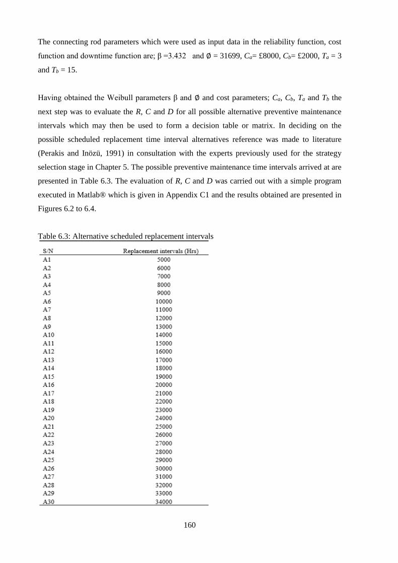
160

The connecting rod parameters which were used as input data in the reliability function, cost

function and downtime function are; β =3.432 and ∅ = 31699, Ca= £8000, Cb= £2000, Ta = 3

and Tb = 15.

Having obtained the Weibull parameters β and ∅ and cost parameters; Ca, Cb, Ta and Tb the

next step was to evaluate the R, C and D for all possible alternative preventive maintenance

intervals which may then be used to form a decision table or matrix. In deciding on the

possible scheduled replacement time interval alternatives reference was made to literature

(Perakis and Inözü, 1991) in consultation with the experts previously used for the strategy

selection stage in Chapter 5. The possible preventive maintenance time intervals arrived at are

presented in Table 6.3. The evaluation of R, C and D was carried out with a simple program

executed in Matlab® which is given in Appendix C1 and the results obtained are presented in

Figures 6.2 to 6.4.

Table 6.3: Alternative scheduled replacement intervals

161

Figure 6.2: Reliability function against scheduled replacement interval tp

Figure 6.3: Cost function against scheduled replacement interval tp

0

0.2

0.4

0.6

0.8

1

1.2

5000 10000 15000 20000 25000 30000 35000

R(t

p)

tp (Hrs)

0

0.05

0.1

0.15

0.2

0.25

0.3

0.35

0.4

0.45

5000 10000 15000 20000 25000 30000 35000

C(t

p)

(£)

tp (Hrs)

162

Figure 6.4: Downtime function against scheduled replacement interval tp

From the results in Figures 6.2, 6.3 and 6.4 it is obvious that the three decision criteria are in

conflict with one another making it difficult to select the optimum preventive replacement

interval. For example: the maintenance practitioner would prefer to maintain the plant with

the highest possible reliability and, as such for the reliability function in Figure 6.2 the

optimum preventive maintenance interval is 5000hrs; however considering the cost function

in Figure 6.3, the optimum replacement interval will occur at the least possible cost and in this

case the preferred maintenance interval is 18,000hrs and finally for the downtime function in

Figure 6.4 the maintenance practitioner would prefer to operate the plant with the least

possible plant downtime and from this analysis the optimum solution would be to carry out

replacement at an interval of 16,000hrs. In such a conflicting scenario, the use of an MCDM

method becomes crucial in order to arrive at a compromise solution. As previously stated, the

use of the TOPSIS method is proposed in this research in selecting the most appropriate

preventive replacement alternative interval. In the TOPSIS technique the first step is to form

the decision matrix which is achieved from the results generated for R, C and D for scheduled

replacement intervals A1 to A30 as presented in Table 6.4.

0

0.0001

0.0002

0.0003

0.0004

0.0005

0.0006

0.0007

5000 10000 15000 20000 25000 30000 35000

D(t

p)

tp (Hrs)

163

Table 6.4: decision matrix for connecting rod

Replacement intervals (tp) tp(hrs) Rtp Ctp(£) Dtp(hrs)

A1 5000 0.998234 0.402036 0.000604

A2 6000 0.996702 0.336712 0.000507

A3 7000 0.994408 0.290747 0.000439

A4 8000 0.991171 0.257035 0.000389

A5 9000 0.986803 0.231631 0.000352

A6 10000 0.981108 0.212175 0.000324

A7 11000 0.973894 0.197167 0.000303

A8 12000 0.964970 0.185607 0.000287

A9 13000 0.954153 0.176806 0.000276

A10 14000 0.941272 0.170267 0.000268

A11 15000 0.926174 0.165626 0.000263

A12 16000 0.908729 0.162604 0.000261

A13 17000 0.888834 0.160983 0.000262

A14 18000 0.866420 0.160589 0.000264

A15 19000 0.841456 0.161276 0.000268

A16 20000 0.813957 0.162918 0.000274

A17 21000 0.783981 0.165407 0.000281

A18 22000 0.751638 0.168643 0.000289

A19 23000 0.717090 0.172532 0.000298

A20 24000 0.680550 0.176986 0.000309

A21 25000 0.642279 0.181920 0.000320

A22 26000 0.602586 0.187251 0.000332

A23 27000 0.561822 0.192896 0.000344

A24 28000 0.520369 0.198773 0.000357

A25 29000 0.478633 0.204805 0.000370

A26 30000 0.437038 0.210912 0.000383

A27 31000 0.396005 0.217019 0.000395

A28 32000 0.355949 0.223053 0.000408

A29 33000 0.317263 0.228948 0.000420

A30 34000 0.280303 0.234641 0.000432

After the formation of the decision matrix, the next step was to use the MCDM tool in ranking

of the alternative maintenance intervals. However prior to the use of the MCDM tool, the

weight of each decision criterion had to be determined. As previously explained, a

combination of AHP and the variance weighting method was used in this research. The results

of R, C and D obtained from the AHP and the variance technique together with the

combination of the two techniques (compromise weighting technique) are presented in Table

6.5 and Figure 6.5.

164

Table 6.5: Combined weight technique comparison with others

Figure 6.5: combine weight technique comparison with others

The evaluated compromise weights of R, C and D together with data in the decision matrix in

Table 6.4 were then used as input data for the TOPSIS analysis. The first step in the TOPSIS

analysis was the normalisation of the decision matrix in Table 6.4 using Eq. (3.6). The

weighted normalised matrix was then obtained by multiplying the normalised decision matrix

by the decision criteria weights. Applying Eq. (3.10) and (3.11), positive and negative ideal

solutions were obtained and the results are presented in Table 6.6. Using Eq. (3.12) and (3.13)

the separation of each of the alternative replacement interval from the positive and negative

ideal solutions were then evaluated. Finally, the relative closeness of each alternative

replacement interval to the positive ideal solution was evaluated using Eq. (3.14) and the

results together with their corresponding rankings are presented in Table 6.7 and Figure 6.6.

Table 6.6: Positive and negative ideal solution

Criteria Negative ideal Positive ideal

Reliability 0.2083 0.9982

Cost 0.4011 0.1605

Downtime 0.0006 0.0003

0

0.1

0.2

0.3

0.4

0.5

0.6

0.7

0.8

R C D

We

igh

ts

Decision criteria

AHP

Variance

compromise

165

Table 6.7: Relative closeness to positive solution and ranking

Replacement

alternatives dp Rank

A1 0.7352 16

A2 0.7932 14

A3 0.8401 11

A4 0.8777 9

A5 0.9073 6

A6 0.9293 4

A7 0.9427 2

A8 0.9458 1

A9 0.9387 3

A10 0.9245 5

A11 0.9058 7

A12 0.8835 8

A13 0.8580 10

A14 0.8293 12

A15 0.7973 13

A16 0.7622 15

A17 0.7240 17

A18 0.6828 18

A19 0.6391 19

A20 0.5930 20

A21 0.5452 21

A22 0.4962 22

A23 0.4469 23

A24 0.3979 24

A25 0.3504 25

A26 0.3056 26

A27 0.2652 27

A28 0.2306 28

A29 0.2036 29

A30 0.1854 30

166

Figure 6.6: Relative closeness to positive ideal and ranking

From Table 6.7 and Figure 6.6 it is obvious that the optimum solution is A8 (12000hrs)

having the highest TOPSIS performance index of 0.9452. The implication is that for this

system, at every interval of 12000hrs, an equivalent of 500 days, the maintenance practitioner

should replace the connecting rod in the marine diesel engine at a cost of 0.18543 per unit

time, reliability of 0.96497 and resulting downtime per unit time of 0.00029. However this

interval can vary from system to system depending on the input parameters into the model

which is controlled by the system age, system failure distribution (such as Weibull, normal

and exponential distribution) demand, prevailing cost factor, maintenance practitioner opinion

and the environment of the operation of the system. This leads to a sensitivity study carried

out to see how the various factors affect the optimum choice.

0

5

10

15

20

25

30

35

0.0000

0.1000

0.2000

0.3000

0.4000

0.5000

0.6000

0.7000

0.8000

0.9000

1.0000

A1

A3

A5

A7

A9

A1

1

A1

3

A1

5

A1

7

A1

9

A2

1

A2

3

A2

5

A2

7

A2

9

Ran

k

dp

Alternative replacement intervals

dp

Rank

167

6.3.3 Sensitivity study

The sensitivity analysis was performed by varying parameters that were used as inputs into

the reliability, cost and downtime cost functions. This was firstly to ascertain the impact of

the input variables on the individual functions; R (tp), C (tp) and D (tp). Secondly it was to

ascertain the impact of the individual input variables in selecting the optimum replacement

interval based on the combination of the three decision criteria, R (tp), C (tp) and D (tp) by the

MCDM technique (TOPSIS). In performing the analysis, the input variables β and ∅ were

increased and decreased by 5%, 10%, 15% and 20% respectively while other variables such

as Ca, Cb, Ta and Tb ratios used were increased and decreased by integer increment.

6.3.3.1 R(tp) sensitivity analysis

The two variables that influence R(tp) are β and ∅ and these factors were increased and

decreased by 5% , 10%, 15% and 20% from the nominal. The results of the sensitivity

analysis based on β and ∅ are presented in Figures 6.7 and 6.8 respectively.

Figure 6.7: Reliability (R(tp)) for sensitivity analysis of β

From Figure 6.7 it can be seen that if only the reliability function was the deciding factor for

selecting the optimum replacement interval, then the optimum solution is unchanged for the

nine cases because the maintenance practitioner will always prefer the highest possible

0.00000

0.20000

0.40000

0.60000

0.80000

1.00000

1.20000

A 1 A 3 A 5 A 7 A 9 A 1 1 A 1 3 A 1 5 A 1 7 A 1 9 A 2 1 A 2 3 A 2 5 A 2 7 A 2 9

R(t

p)

tp(intervals)

5%

10%

15%

20%

-5%

-10%

-15%

-20%

0%

168

reliability for the operation of the system. For the nine cases, the highest reliability is

approximately one at a time interval for carrying out maintenance of A1 (5000hrs). It is also

worth mentioning from the graph that the lowest possible reliability for the nine cases is

almost the same. One can then conclude that the rate of decrease of reliability of this system

with age or time for any value of the factor β is almost constant.

Figure 6.8: Reliability (R(tp)) for sensitivity analysis of ∅

Again increasing or decreasing the value of ∅ as shown in Figure 6.8, does not change the

optimum interval (A1) for performing replacement maintenance as the maintenance

practitioner would prefer to maintain the highest possible reliability. Although from the

graph, the highest possible reliability i.e. approximately one for the nine cases is the same, the

lowest possible varies greatly for the nine cases, ranging from 0.064859 when ∅ was

decreased by 20% to 0.34103 when ∅ was increased by 20%. It can be concluded that

reliability decreases with age i.e. A1 to A30 and the rate of decrease depends greatly on the

value of ∅. In terms of the overall ranking of the scheduled replacement interval alternatives

using MCDM based on the three decision criteria; R(tp), C(tp) and D(tp), the impact of ∅ will

be greater than β since reliability is more sensitive to ∅ than β when Figures 6.7 and 6.8 are

compared.

6.3.3.2 C (tp) sensitivity analysis

For the cost model C(tp), the optimum preventive maintenance interval (tp) is the interval

with the least possible cost. The input parameters that influence the output of this cost model

0

0.2

0.4

0.6

0.8

1

1.2

A 1 A 3 A 5 A 7 A 9 A 1 1 A 1 3 A 1 5 A 1 7 A 1 9 A 2 1 A 2 3 A 2 5 A 2 7 A 2 9

R(t

p)

tp(intervals)

5%10%15%20%-5%-10%-15%-20%0%

169

are ∅, β, Ca, Cb, Ta and Tb and as such a sensitivity analysis was performed on these input

variable.

For the sensitivity analysis performed on β, the original value was increased and decreased by

5%, 10%, 15% and 20% and the results are presented in Figure 6.9.

Figure 6.9: Cost per unit time for sensitivity analysis of β

From Figure 6.9, the optimum replacement interval (tp) A14 (18,000hrs) remained unchanged

when β was increased by up to 20% and decreased by up to 20%. However there was a small

decrease in cost when β was increased from the original value by up to 20% and a small

increase in cost when β was decreased by up to 20%.

In order to examine the effect of the variation of ∅ on the cost model, the variable was again

increased and decreased by 5%, 10%, 15% and 20%. The result of the sensitivity analysis is

presented in Figure 6.10. From the figure it is obvious that ∅ has a greater impact on cost than

β, and unlike the analysis of β with respect to cost where the optimal replacement interval

remained unchanged, the optimum interval for ∅ changes as the parameter is increased or

decreased. As the variable ∅ was increased from the original value (0%) by 5%, 10%, 15%,

the optimal interval changed from A14 to A15, A16, and A17 respectively with a

corresponding decrease in the cost for performing preventive maintenance. However when the

variable was increased from 15% to 20% the optimum interval was unchanged. On the other

hand, when the variable ∅ was decreased by 5%, 10%, 15% and 20% there was a

corresponding decrease in the optimum replacement interval by a factor of one with a

0.00000

0.05000

0.10000

0.15000

0.20000

0.25000

0.30000

0.35000

0.40000

0.45000

A 1 A 3 A 5 A 7 A 9 A 1 1A 1 3A 1 5A 1 7A 1 9A 2 1A 2 3A 2 5A 2 7A 2 9

C(t

p)

tp(intervals)

5%

10%

15%

20%

-5%

-10%

-15%

-20%

0%

170

marginal increase in the cost of carrying out scheduled replacement maintenance. For

example when the original value of ∅ was decreased by 5% the alternative replacement

interval changed from A14 (18,000hrs) to A13 (17,000hrs) and when ∅ decreased by 10% it

changes to A12 (16,0000hrs).

Figure 6.10: Cost per unit time (C(tp)) for sensitivity analysis of ∅

Another input parameter whose impact on the output of the cost model was tested is the cost

ratio i.e. the ratio of the cost of maintenance as result of breakdown (Ca) to the cost of

preventive maintenance (Cb). The ratio was varied ranging from 2 to 8 in order to measure

the effect on the output of the cost model as shown in Figure 6.11. It can be seen from Figure

6.11 that as the ratio increased the optimum replacement interval decreased with an increase

in the cost of performing the maintenance task. For example the optimum interval when the

ratio of Ca to Cb is set at 2 is A21 (25,000hrs) at a cost per unit time of £0.12; when the ratio

is set at 3 the optimum interval (tp) changes to A16 (20000hrs) at a cost per unit time of £0.14.

From this analysis it is obvious that the cost model is more sensitive to the ratio of Ca to Cb

than the variable ∅ as the decrease in the optimum interval (tp) is more sudden.

Finally, the impact of changes in the ratio of Tb to Ta on the cost model was determined and in

the scenario the ratios were varied from 2 to 9 as presented in Figure 6.12. The figure shows

that changes in the ratio did not result in any change in the optimal replacement interval as in

all the cases the interval remained at A14 (12,000hrs) with a very marginal increase in cost

per unit time.

0

0.05

0.1

0.15

0.2

0.25

0.3

0.35

0.4

0.45

A 1 A 3 A 5 A 7 A 9 A 1 1A 1 3A 1 5A 1 7A 1 9A 2 1A 2 3A 2 5A 2 7A 2 9

C(t

p)

tp (intervals)

5%

10%

15%

20%

-5%

-10%

-15%

-20%

0%

171

Figure 6.11: Cost per unit (C(tp)) for sensitivity analysis of Cost ratio

Figure 6.12: Cost per unit time (C(tp)) for sensitivity analysis of ratio of Tb to Ta

6.3.3.3 D(tp) sensitivity analysis

In order to ascertain the influences of the of the input variables such as β, ∅, Ca, Cb, Tb and Ta

on the D(tp) model a sensitivity analysis was performed by changing these variables by a

certain quantity.

0

0.05

0.1

0.15

0.2

0.25

0.3

0.35

0.4

0.45

0.5

A 1 A 3 A 5 A 7 A 9 A 1 1A 1 3A 1 5A 1 7A 1 9A 2 1A 2 3A 2 5A 2 7A 2 9

C(t

p)

tp(intervals)

Ca:Cb=4

Ca:Cb=5

Ca:Cb=6

Ca:Cb=7

Ca:Cb=8

Ca:Cb=3

Ca:Cb=2

0

0.05

0.1

0.15

0.2

0.25

0.3

0.35

0.4

0.45

A1 A3 A5 A7 A9 A11A13A15A17A19A21A23A25A27A29

C(t

p)

tp(intervals)

Tb:Ta=5

Tb:Tb=6

Tb:Ta=7

Tb:Ta=8

Tb:Ta=9

Tb:Ta=4

Tb:Ta=3

Tb:Ta=2

172

For the sensitivity investigation performed on β, the original value was increased and

decreased by 5%, 10%, 15% and 20% and the results are presented in Figure 6.13. The results

show that the optimum replacement interval (tp) remains the same in the nine scenarios

however with a gradual increase in cost per unit time when β varied from -5% up to -20% and

gradual decrease in cost per unit time when β varied from 5% up to +20%. In a similar

fashion, a sensitivity analysis was performed by decreasing and increasing ∅ over the range of

5% to 20%. The result of the sensitivity analysis is as shown in Figure 6.14. The result of this

investigation shows that an increase in the variable ∅ resulted in a small increase in the

replacement interval and a decrease in the value of ∅ produced a decrease in the replacement

interval.

Figure 6.13: Downtime per unit time for sensitivity analysis of β

0.00000

0.00010

0.00020

0.00030

0.00040

0.00050

0.00060

0.00070

A 1 A 3 A 5 A 7 A 9 A 1 1 A 1 3 A 1 5 A 1 7 A 1 9 A 2 1 A 2 3 A 2 5 A 2 7 A 2 9

D(t

p)

tp(intervals)

5%

10%

15%

20%

-5%

-10%

-15%

-20%

0%

173

Figure 6.14: Downtime per unit time (C(tp)) for sensitivity analysis of ϕ

Finally, the D(tp) model sensitivity analysis was performed by varying the ratio of Tb to Ta

over the range of 2 to 9. From the result shown in Figure 6.15 it can be seen that when the

ratio increased there was a reduction in the optimum replacement interval, however with an

increase in cost per unit time of performing the maintenance task.

Figure 6.15: Downtime per unit (D(tp)) for sensitivity analysis of ratio of Tb to Ta

0

0.0001

0.0002

0.0003

0.0004

0.0005

0.0006

0.0007

A 1 A 3 A 5 A 7 A 9 A 1 1 A 1 3 A 1 5 A 1 7 A 1 9 A 2 1 A 2 3 A 2 5 A 2 7 A 2 9

D(t

p)

tp(intervals)

5%

10%

15%

20%

-5%

-10%

-15%

-20%

0%

0

0.0001

0.0002

0.0003

0.0004

0.0005

0.0006

0.0007

0.0008

A1 A3 A5 A7 A9 A11A13A15A17A19A21A23A25A27A29

D(t

p)

tp(intervals)

Tb:Ta=5

Tb:Ta=6

Tb:Ta=7

Tb:Ta=8

Tb:Ta=9

Tb:Ta=4

Tb:Ta=3

Tb:Ta=2

174

6.3.4 Impact of input parameters variations on the overall ranking of replacement

interval alternatives

Having established the impact of changes to the individual input parameters on the three

decision criteria R(tp), C(tp) and D(tp), the next step was to determine the impact of the

variations of input parameters on the overall ranking of the replacement alternative intervals.

As previously explained, when R(tp), C(tp) and D(tp) are used simultaneously as decision

criteria to determine the optimum replacement intervals, an MCDM technique is appropriate

for selecting the optimal alternative interval and in this research TOPSIS was used. The

TOPSIS performance index for all replacement alternative intervals was generated as the

individual input parameters were varied and based on the TOPSIS performance index,

replacement alternative intervals were ranked.

6.3.4.1 Impact of β variations on the overall ranking of replacement interval

alternatives

Firstly the impact of the variation of β on the overall ranking of the alternative replacement

intervals was considered. The TOPSIS performance index was obtained for all replacement

interval alternatives as input parameter β was increased and decreased by 5%, 10%, 15% and

20%. The result obtained is presented in Table C1 in Appendix C2 and based on these, the

TOPSIS performance index and scheduled replacement interval alternatives were ranked as

shown in Figure 6.16 a &b and Table C2 in appendix C2. Note Figure 6.16b is only a section

of Figure 6.16a and it’s presented to clearly shown how replacement (maintenance)

alternative intervals vary with increase or decrease of parameter β.

175

Figure 6.16 a: Ranking of sensitivity analysis of β

Figure 6.16b: Ranking of sensitivity analysis of β

From Figure 6.16a and Table C2 it can be seen that the optimal replacement interval for the

original value of β (0%) was A8 (12,000hrs) having rank of 1. However as the value of β was

increased by 10% the optimal replacement interval remained unchanged. It was not until β

was increased by 15% and 20% that the optimal interval became A9 (13,000hrs). On the other

0

5

10

15

20

25

30

35

A1

A2

A3

A4

A5

A6

A7

A8

A9

A1

0

A1

1

A1

2

A1

3

A1

4

A1

5

A1

6

A1

7

A1

8

A1

9

A2

0

A2

1

A2

2

A2

3

A2

4

A2

5

A2

6

A2

7

A2

8

A2

9

A3

0

Ran

k

Replacement alternative interval (tp)

-5%

-10%

-15%

-20%

0%

5%

10%

15%

20%

0

2

4

6

8

10

12

14

16

18

20

A1 A2 A3 A4 A5 A6 A7 A8 A9 A10 A11 A12 A13 A14 A15 A16 A17 A18

Ran

k

Replacement alternative interval (tp)

-5%

-10%

-15%

-20%

0%

5%

10%

15%

20%

176

hand, as the value of β was decreased by 5% the optimal replacement interval changed to A7

(11,000hrs) and it further changed to A6 (10,000) when the value of β was decreased by 20%.

To summarise, the higher the value of β the higher the replacement interval and the lower the

value of β the lower the replacement interval. An additional conclusion is that in all the

scenarios, whether increasing or decreasing the value of β, the optimal replacement interval

varied by relatively small amount as the change was over the range A6 - A9.

6.3.4.2 Impact of ∅ variations on the overall ranking of replacement interval alternatives

The impact of ∅ on the overall ranking of alternative replacement intervals was performed by

decreasing and increasing the values of ∅ by 5%, 10%, 15% and 20% and using the results

obtained in each scenario as input to the TOPSIS methodology which was evaluated using

TOPSIS. The TOPSIS performance indices generated in the nine scenarios are presented in

Table C3 in Appendix C2. On the basis of the TOPSIS performance indices, the replacement

alternative intervals were ranked and the results are presented in Table C4 in Appendix C2

and Figure 6.17.

Figure 6.17: Ranking of sensitivity analysis of ϕ

From Table C4 in Appendix C2 and Figure 6.17, it can be seen that the sensitivity analysis

results obtained for ∅ are very similar to the results generated for β since as the value of ∅

increased the replacement interval increases and as the value decreases the replacement

interval decreased just as in the case of β. However, the corresponding changes in the

0

5

10

15

20

25

30

35

A1

A2

A3

A4

A5

A6

A7

A8

A9

A1

0

A1

1

A1

2

A1

3

A1

4

A1

5

A1

6

A1

7

A1

8

A1

9

A2

0

A2

1

A2

2

A2

3

A2

4

A2

5

A2

6

A2

7

A2

8

A2

9

A3

0

Ran

k

Replacement alternative interval (tp))

_20%

-15%

-10%

-5%

0%

5%

10%

15

20%

177

replacement interval to the changes in ∅ are larger than the response to the changes in β. In

other words, the ranking model is more sensitive to changes in ∅ than β.

6.3.4.3 Impact of cost ratio variations on the overall ranking of replacement interval

alternatives

The sensitivity analysis was perform on cost ratio to determine the effect that changes of the

ratio of Ca to Cb would have on the overall ranking of replacement interval alternatives. The

ratio of Ca to Cb ranging from 2 to 8 was applied in carrying out the investigation. The

TOPSIS performance index obtained for all the replacement interval alternatives for all eight

scenarios and their corresponding rankings are presented in Tables C5 and C6 in Appendix

C2. The graphical representation of the ranking of all alternatives are shown in Figure 6.18a

& b. Note Figure 6.18b is only a section of Figure 6.18a and it’s presented to clearly shown

how replacement (maintenance) alternative intervals vary with increase or decrease of cost

ratio.

From Table C6 in Appendix C2 and Figure 6.18a it can be seen that as the ratio of Ca to Cb

increased up to 5 there was a reduction in the replacement interval. Increases beyond 5

resulted in no further change across the range of scenarios i.e. the ratio of Ca to Cb ranging

from 2 to 8, only three replacement interval choices were obtained (A9, the optimal

replacement interval obtained for Ca:Cb =2, A8 the optimal replacement interval obtained for

Ca:Cb=3 to 4 and A7 the optimal replacement interval obtained for Ca:Cb=5 to 8). It can be

concluded that as the ratio increases, the replacement interval decreases up to a point and then

remains constant. When compared to β and ∅ the cost ratio has a smaller impact on the

ranking of replacement interval alternatives.

178

Figure 6.18a: Ranking of sensitivity analysis of cost ratio

Figure 6.18b: Ranking of sensitivity analysis of cost ratio

0

5

10

15

20

25

30

35

A1

A2

A3

A4

A5

A6

A7

A8

A9

A1

0

A1

1

A1

2

A1

3

A1

4

A1

5

A1

6

A1

7

A1

8

A1

9

A2

0

A2

1

A2

2

A2

3

A2

4

A2

5

A2

6

A2

7

A2

8

A2

9

A3

0

RA

NK

MAINTENANCE ALTERNATIVE INTERVAL (TP)

Ca:Cb=2

Ca:Cb=3

Ca:Cb=4

Ca:Cb=5

Ca:Cb=6

Ca:Cb=7

Ca:Cb=8

0

2

4

6

8

10

12

14

16

18

20

1 2 3 4 5 6 7 8 9 10 11 12 13 14 15 16 17 18

RA

NK

MAINTENANCE ALTERNATIVE INTERVAL (tp)

Ca:Cb=2

Ca:Cb=3

Ca:Cb=4

Ca:Cb=5

Ca:Cb=6

Ca:Cb=7

Ca:Cb=8

179

6.3.4.4 Impact of ratio Tb to Ta variations on the overall ranking of replacement

interval alternatives

In order to determine the impact that variation of the ratio Tb to Ta would have on the overall

ranking of replacement interval alternatives, the ratio of Tb to Ta was varied from 2 to 9 and

the TOPSIS performance index generated for the replacement interval alternatives for the

eight scenarios. The results are presented in Table C7 in Appendix C2. The performance

index for the replacement interval alternatives in the nine scenarios were ranked and the

results are presented in Table C8 in Appendix C2 and Figure 6.19. It is obvious from the table

and graph that the optimal replacement interval for the scenarios remained unchanged with

the exception of the first scenario (Tb to Ta equal to 2). When compared to the other input

parameters the Tb to Ta ratio has less impact on the overall ranking of replacement interval

alternatives.

Figure 6.19: Ranking of sensitivity analysis of ratio of Tb to Ta

0

5

10

15

20

25

30

35

A1

A2

A3

A4

A5

A6

A7

A8

A9

A1

0

A1

1

A1

2

A1

3

A1

4

A1

5

A1

6

A1

7

A1

8

A1

9

A2

0

A2

1

A2

2

A2

3

A2

4

A2

5

A2

6

A2

7

A2

8

A2

9

A3

0

RA

NK

MAINTENANCE TIME INTERVAL (TP)

Tb:Ta=2

Tb:Ta=3

Tb:Ta=4

Tb:Ta=5

Tb:Ta=6

Tb:Ta=7

Tb:Ta=8

Tb:Ta=9

180

6.4 Summary

For safe and reliable operation of marine machinery systems at reasonable cost there needs to

be in place an efficient maintenance system. However in making maintenance decisions,

different parties are involved and the decisions are usually based on certain criteria which are

always in conflict with one another. In resolving such conflicts the multi-criteria decision

making technique is usually suitable. In this research, decision criteria such as reliability, cost

and downtime were considered as the basis for selecting the optimum preventive replacement

interval for marine machinery systems. Since the three decision models are in conflict with

one another, the outputs were aggregated with the aid of MCDM techniques. In order to

demonstrate the applicability of the methodology, failure data obtained from secondary

sources and estimated cost data for the connecting rod of a marine diesel engine were used as

input data. The result of the investigation revealed the following:

(1) For the data considered, the optimum replacement interval for performing

maintenance tasks on the connecting rod of the marine diesel engine is 12,000hrs. However

this is not fixed as the interval could vary depending on the operating environment of the

system, the age of the system, cost of replacement at breakdown, cost of preventive

replacement and type of failure distribution.

(2) If the Weibull distribution is the failure distribution for the system, the scale

parameter, ∅, has a greater impact on the three models than the shape parameter, β. However

for the cost model the ratio of Ca to Cb has the greatest impact. For the downtime model, the

ratio of Tb to Ta has the greatest impact followed by ∅ while β has the least impact.

(3) ∅ has the greatest influence on the overall ranking of replacement interval alternative.

The ratio of Tb to Ta has the least impact on the overall ranking of replacement intervals.

(4) Increasing the values of parameters such as ∅ and β will result in a corresponding

increase in the replacement interval and reducing the value will result in a reduction in the

replacement interval.

From the result of this analysis the proposed methodology is simple and robust. The approach

in this research has an advantage over the technique applied by some authors for land based

systems as the criteria weight evaluation model is flexible with both objective and subjective

components. The proposed methodology is not limited to application to marine machinery

systems as it capable of solving other engineering system problems if provided with the

appropriate input data.

181

Chapter 7 Inspection Interval Determination

7.1 Introduction

One of the maintenance strategy options for maintaining components of a marine system is

scheduled on-condition task which was referred to as Offline-Condition Based Maintenance

(OFCBM) in Chapter 5. As previously stated, scheduled on-condition task is the inspection

carried out on plant systems to monitor their performance degradation. Once it has been

established that the optimum maintenance strategy for mitigating failure of a particular

equipment item of the system is scheduled on-condition task, the next task is to determine the

interval for performing the maintenance task.

Based on the literature review in Chapter 2, the most promising technique for determining the

optimum interval for carrying out inspection is the delay time model. However most of the

delay-time model applications for inspection interval determination discussed in the literature

are based on a single model such as the use of cost or downtime in optimising inspection.

However a few cases considered a combination of two models in deciding the inspection plan

for either a single unit or multi-unit system. In these few cases, the optimum inspection

intervals obtained from the individual models were close and, as such, reaching a compromise

solution was straightforward without resorting to special MCDM tools. Nevertheless in most

real life applications the decision criteria results may not be close and in such a scenario

reaching a compromise solution becomes challenging. For cases of this nature, the use of

multi-criteria tools such as PROMETHEE, TOPSIS, Elimination Et Choix Traduisant La

REalite (ELECTRE) and Multi-Attribute Utility Theory (MAUT) becomes imperative.

Additionally the use of such tools make it possible to include the opinion of maintenance

practitioners in the decision making process. The use of the MAUT method specifically has

an additional benefit of integrating the risk perception of the maintenance practitioners into

the decision making process. Considering the benefits of both delay model and MAUT

techniques, a combination of the two methods is proposed for determining the inspection

interval for marine machinery systems.

The Chapter is organised as follows: In Section 7.2 a background study of the delay time

model is discussed; Section 7.3 presents the proposed methodology for determining the

182

optimum inspection interval; in Section 7.4 the case of the water cooling pump is presented to

demonstrate the proposed methodology. Finally the conclusion is presented in Section 7.5

7.2 Delay time model background

In determining the maintenance strategy of marine systems using the RCM methodology,

some equipment items are more effectively maintained by scheduled inspection or scheduled

inspection in combination with other maintenance tasks. The essence of inspection is to

ascertain the true condition of an item and as such it’s similar to online condition based

maintenance. The difference is that while inspection is carried out by maintenance personnel,

online condition based monitoring is carried out through the use of diagnostic tools which

continually monitor the condition of the equipment. In the course of performing inspection

activities, if a defect is found, a repair or replacement task is schedule and if possible executed

immediately to prevent the equipment from further deterioration. If inspections are not carried

out, defects may go unnoticed which can result in catastrophic system failure with severe

economic loss for the company. However even if inspection tasks are performed, if they are

not properly timed, defects can still occur between successive intervals. It is obvious then that

the determination of the optimal inspection interval is central to the effective operation of any

marine machinery system. Conventionally the inspection interval is determine by maintenance

practitioners relying on experience and/ or on the equipment manufacturers’ recommendation,

the result being far from optimal and also conservative (Christer et al., 1997).

An inspection task as an alternative maintenance approach can only be beneficial if there is a

sufficient period between the time that the defect is observed and the actual time of failure of

the equipment. The time interval between when a defect becomes identifiable and the actual

time of failure is referred to as the delay time (hf). Based on this concept, Christer proposed

the Delay Time model (Christer et al., 1997) for determining the inspection interval of an

equipment item. The delay time is the most appropriate time to carry out an inspection on a

marine machinery system. Figure 7.1 is used to illustrate the delay time concept.

183

Figure 7.1: Delay time concept showing a defect’s initial points and failure points

Figure 7.1 shows multiple points of failure, both initial and actual points where failure occurs

and also two different inspection plans for the marine machinery system in question. It is

obvious from the figure that if the inspection of the system is performed at an interval of B a

lot of failures will happen in the system since most of the defects would have resulted in

actual failure. Alternatively inspection plan A would result in detecting virtually all of the

defects before the actual failure of the system could occur. The key to achieving maximum

success in mitigating catastrophic failure of a marine machinery system is to have a proper

understanding of the delay time (hf) of the system such that maintenance can be performed

within this period.

Based on Christer and Waller (1984a), a defect occurring within a period of (0, T) in a marine

machinery system has a delay time, hf and hf has a probability density function of f(hf). If

failure of the machinery system occurs at a period (0, T-hf) the maintenance (repair or

replacement) carried out is referred to as breakdown maintenance otherwise the maintenance

is inspection maintenance. For the marine machinery system, if all possible values of hf are

added up, according to Christer and Waller (1984a), the probability of a defect occurring as a

breakdown failure is:

𝐵(𝑇) = ∫𝑇 − ℎ𝑓

𝑇

𝑇

0

𝑓(ℎ𝑓)ℎ𝑓 (7.1)

The above Equation was established based on the following assumptions:

184

(1) Inspection is performed at regular intervals

(2) Defects discovered during inspection are repaired

(3) Perfect inspection meaning all defects are discovered during inspection

(4) Arrival rate of defects is constant

However it is worth noting that some of these assumptions may not be realistic in practical

situations. For example, it may not be possible to identify all defects during inspection as

some defects could be hidden although the system performance degradation may have started

during inspection. Some of these assumptions are made to ease the modelling of the system

and for ease of computation of the models.

Detailed information on the delay time concept and its application in marine and other related

industries for the purpose of optimising maintenance, was discussed in the literature section.

7.3 Proposed inspection interval determination methodology

In this research, the delay time model was used in conjunction with MCDM techniques in

order to determine the optimum inspection interval for marine machinery equipment. The

MCDM techniques are used in aggregating the expected cost, expected downtime and

reputation models. The weights of the decision criteria were evaluated with respect to

maintenance practitioners’ preference. Hence a flexible weighting technique has been

developed for this purpose. The decision criteria considered simultaneously in deciding the

optimum inspection interval using the delay time technique are; Downtime per unit time D(T)

and Cost per unit time C(T) and expected Reputation per unit time R(T). The flowchart of the

proposed methodology for selecting appropriate inspection intervals for the marine machinery

system is presented in Figure 7.2.

The methodological steps are as follows:

Step (a) the system to be investigated is determined and is usually broken down into sub-

systems and components. Next the system is thoroughly studied to identify dominant failures

and corresponding consequences. Various techniques such as, group brainstorming, FMEA

and FTA can be applied to determine dominant failures, causes and the chances of the failures

occurring. In this research, the FMEA technique was chosen for this purpose. Once the

185

dominate failures have been identified, data is gathered to be applied as input into a

mathematical model for optimising the inspection interval such that system failure can be

eliminated or minimised. The data that can be applied for delay time model analysis may be

subjective /and or objective. Objective data is generally preferable however, if it is lacking in

quality and quantity, subjective data can be applied. Objective data is obtained from

maintenance and failure data records from the marine industry. In most cases, this data is not

available because of the nature of the environment and sometimes due to commercial

sensitivity. Subjective data on the other hand is obtained by developing questionnaires which

are used in gathering information relating to maintenance and equipment failures from marine

maintenance personnel, vessel crews and management.

Step (b) The three mathematical models based on the delay time concept; D(T), C(T) and

R(T) are evaluated by using data collected in step (a). Common to the three Delay Time

Analysis (DTA) models are variables such as B(T), downtime as a result of inspection, 𝜕 ,

and arrival rate of defects per unit time, 𝑘𝑟. To determine B(T), a failure mode is chosen and

from failure records, the initial point of failure is determined. This is followed by the

determination of the distribution of the delay time of failure which may be a normal,

exponential or Weibull distribution. Once the distribution has been estimated, the parameters

of the distributions may be determined. These parameters are then used as input into the B(T)

model to calculate its value. Having known values of B(T), 𝜕 and 𝑘𝑟 , D(T) is evaluated. To

evaluate C(T) other variables such as costs of breakdown, inspection repairs and inspection

are needed in addition to B(T), 𝜕 and 𝑘𝑟 and finally to evaluate R(T) parameters such as Rbr

and Rii are needed in addition to B(T), 𝜕 and 𝑘𝑟.

Step (c) C(T), D(T) and R(T) are evaluated for every value of T and used to form a decision

matrix, xij (m x n), as presented in Table 7.1, where m is the number of alternative inspection

Ti , and n is the number of decision criteria. In this case, the decision criteria are C(T), D(T)

and R(T).

Step (d) Determination of decision criteria weight: The pairwise comparison judgment

obtained from the experts for the decision criteria is used as the input into the AHP evaluation

technique to calculate weights of decision criteria.

186

Figure 7.2: Flow of the integrated MCDM and Delay time model for inspection selection

187

Table 7.1: Inspection interval alternatives decision table

Step (e) Ranking of inspection alternatives: The maintenance strategy alternatives are ranked

using Elimination Et Choix Traduisant La REalite (ELECTRE) and Multi-Attribute Utility

Theory (MAUT).

Step (f) the ranking obtained from both methods are compared and an optimum strategy is

then determined

7.3.1 Develop delay time concepts models

The assumption in this research is that the delay times of failure for the marine machinery

systems components follow a Weibull distribution, therefore 𝑓(ℎ𝑓) is represented as follows:

𝑓(ℎ𝑓) =𝛽

∅(ℎ𝑓

∅)

𝛽−1

𝑒𝑥𝑝 [−(ℎ𝑓

∅)

𝛽

] (7.2)

On the basis of Eq. (7.2) the B(T) model, which is the probability that defects will be repaired

as breakdown repairs in Eq. (7.1) can be represented as follows:

𝐵(𝑇) = ∫𝑇 − ℎ𝑓

𝑇

𝑇

0

𝛽

∅(ℎ𝑓

∅)

𝛽−1

𝑒𝑥𝑝 [−(ℎ𝑓

∅)

𝛽

] 𝑑ℎ𝑓 (7.3)

188

7.3.1.1 Downtime models

The expected downtime per unit possible time of inspection using the delay time approach

can be presented as follows (Christer and Waller, 1984a):

𝐷(𝑇) =𝜕 + 𝑘𝑟𝑇𝐵(𝑇)𝑑𝑎

𝑇 + 𝜕 (7.4)

Where

T = Inspection time interval

𝜕 = Downtime as a result of inspection

𝑑𝑎 = Average downtime due to breakdown repair

ℎ𝑓= Delay time

𝑘𝑟= Arrival rate of defects per unit time

If Eq. (7.3) is substituted in to Eq. (7.4), D(T) will be represented as:

𝐷(𝑇) =

𝜕 + 𝑘𝑟𝑇 {∫𝑇 − ℎ𝑓

𝑇𝑇

0 𝛽∅

(ℎ𝑓

∅)

𝛽−1

𝑒𝑥𝑝 [−(ℎ𝑓

∅)𝛽

] 𝑑ℎ𝑓} 𝑑𝑎

𝑇 + 𝜕 (7.5)

7.3.1.2 Expected Cost model

The downtime model in Eq 7.4 may be modified by including three distinct cost components;

cost of breakdown, cost of inspection repair and cost of inspection, in order to model the

expected cost per unit time function (Christer and Waller, 1984a). The expected cost per unit

time of inspection of a marine machinery system, C(T), is written as follows:

𝐶(𝑇) =[𝑘𝑟𝑇{𝐶𝑏𝑟𝐵(𝑇) + 𝐶𝑖𝑖[1 − 𝐵(𝑇)]} + 𝐶𝑖𝑐]

𝑇 + 𝜕 (7.6)

Where

𝐶𝑏𝑟 = cost of breakdown repair

𝐶𝑖𝑖 = cost of inspection repair

𝐶𝑖𝑐 = cost of inspection

189

The three cost variables each need to be evaluated to be applied as an input into C(T) together

with the delay time parameters. In order to evaluate breakdown repair cost there is a need to

know all of the failure modes of the marine machinery system and the corresponding

consequences of the failure. As previously stated, FMEA has been applied in this research. In

Chapter 4, the consequences of the failure modes were presented whose values were assigned

by experts using an ordinal scale of 1 to 10. These are now expressed in monetary terms. The

cost of breakdown repair is evaluated as the sum of the labour cost (Lc), spare parts cost (Sc),

equipment downtime time cost (Edc), penalty cost (Pc), and dry-docking cost (Ddc) shown as

follows:

𝐶𝑏𝑟 = 𝐿𝑐 + 𝑆𝑐 + 𝐸𝑑𝑐 + 𝑃𝑐 + 𝐷𝑑𝑐 (7.7)

The labour cost can be expressed as the product of the number of maintenance personnel

(Ncm) that will carry out the repair, the pay rate per hour per person (Prm) and the time

duration of repair (Tdm). This is shown as follows:

𝐿𝑐 = 𝑁𝑐𝑚. 𝑃𝑟𝑚. 𝑇𝑑𝑚 (7.8)

The cost of inspection repair is presented as follows:

𝐶𝑖𝑖 = 𝐶𝑖𝑐 + 𝐿𝑐 + 𝑆𝑐 + 𝐸𝑑𝑐 + 𝑃𝑐 (7.9)

It is obvious from Eq. 7.7 and 7.9 that the cost of break down repair and cost of inspection

repair are the same except that (1) inspection cost is included in the cost of inspection repair

and dry-docking cost is excluded from it. The dry-docking cost is excluded from inspection

repair because defects are addressed before the actual failure occurs and so it will not result in

catastrophic failures that can call for unplanned dry-docking of the entire ship system; and (2)

the time duration for performing corrective action during breakdown repair is higher than the

time duration for carrying inspection repair. The time duration for breakdown repair is

generally higher than time taken to perform corrective action for inspection repair because in

breakdown repair the defect may not only have resulted in a particular component failure but

could also result in both secondary and tertiary effects.

190

The cost of inspection 𝐶𝑖𝑐 for the machinery system equipment or component may be

expressed as the product of the number of marine maintenance crew (Nic), their pay rate per

hour (Pr) and the duration for performing the maintenance added to the product of equipment

or component downtime and duration of performing the maintenance, presented as follows:

𝐶𝑖𝑐 = [(𝑁𝑖𝑐 . 𝑃𝑟 ) + 𝐸𝑑𝑐]𝑇𝑑 (7.10)

Where Td is the duration of inspection.

7.3.1.3 Expected Reputation model

With the reputation model, the relationship between the impact of failures on the reputation or

image of the marine industry can be studied. The failure of marine machinery systems can

have a negative impact on the company and as such this model helps in determining the most

appropriate time interval to perform maintenance inspection with the intention of reducing or

eliminating system downtime whilst boosting the reputation of the company. In similar

fashion to developing the cost model and downtime model, the reputation model is presented

as follows:

𝑅(𝑇) =𝑘𝑟𝑇{𝑅𝑏𝑟𝐵(𝑇) + 𝑅𝑖𝑖[1 − 𝐵(𝑇)]}

𝑇 + 𝜕 (7.11)

Where Rbr is the company reputation when a failure correction measure is performed as a

breakdown repair and Rii is the company reputation when failure corrective action is

performed as an inspection repair. In assigning values to the two variables; Rbr and Rii , an

ordinal scale of 1 to 10 is applied by experts. The value assigned is a function of the severity

and the occurrence of the failure. In this case, the worst case scenario was assumed for Rbr

since a breakdown repair scheme may sometimes result in catastrophic damage that may

affect personnel on board ship, marine machinery system equipment and the environment. For

Rii , the best case scenario may be assumed since failures are preventatively mitigated. For the

best case scenario 1 is assigned and for the worst case scenario 8 to 10 can be assigned.

A programme was written in Matlab® to evaluate D(T), C(T), and R(T). The Programme is

given in Appendix D.

191

7.3.2 Decision criteria weighting techniques

The AHP technique for determining the weights of decision criteria; D(T), C(T) and R(T) was

discussed in Chapter 4.

7.3.3 Ranking of time interval tools

The decision making process involves applying simultaneously three decision criteria which

are usually conflicting, in arriving at the most appropriate time interval for inspection of the

marine machinery system. Two MCDM techniques; ELECTRE and MAUT were used and

compared. The methodological steps for these methods are discussed next:

7.3.3.1 ELECTRE method

ELECTRE is the acronym for Elimination and Et Choice Translating Reality, a multi-criteria

technique which utilises the concept of paired comparisons among alternatives with respect to

chosen decision criteria. The method was established by Roy and Vinke (Roy and Vincke,

1981) and has since been modified and applied successfully in addressing multi-criteria

decision problems in different fields. Shanian et al. (2008) utilised the technique in solving a

material selection problem and Sevkli (2010) integrated ELECTRE with a fuzzy logic

technique in addressing a supplier selection problem. In this thesis, the technique has been

used to solve an inspection interval selection problem in the marine environment. The

methodological steps associated with the ELECTRE method as presented in (Anojkumar et

al., 2014) are as follows:

Step 1: Formation of the decision matrix: the process starts with formation of a decision

matrix, X, with alternatives, j with respect to criteria, i. An example of such a decision matrix

with elements xij is presented in Table 7.1.

Step 2: Normalisation of the decision matrix: the normalisation of the decision matrix is

performed in order to convert varying units among different decision criteria into

dimensionless form. The normalisation of the decision matrix xij is carried out as follows:

𝑟𝑖𝑗 = 𝑥𝑖𝑗

√∑ 𝑥𝑖𝑗2𝑚

𝑗=1

, 𝑖 = 1,2… , 𝑛 ; 𝑗 = 1,… ,𝑚 (7.12)

192

Where rij is the normalised matrix

Step 3: determination of the weighted normalised matrix:

The weighted normalised matrix (vij) is obtained as a product of decision criteria weight, wi ,

and the normalised matrix as follows:

𝑣𝑖𝑗 = 𝑤𝑗𝑟𝑖𝑗 , 𝑖 = 1, … , 𝑛 ; 𝑗 = 1,… ,𝑚 (7.13)

Step 4: Determination of the concordance interval matrix: Given a pair of alternatives, Aj and

Ak, the concordance index cI(j, k) can be evaluated as the summation of all weights for those

criteria where weighted normalised score of Aj is greater than or equal to Ak, , as follows:

𝑐𝐼(𝑗, 𝑘) = ∑ 𝑤𝑖 ,

𝑣𝑖(𝑗)≥𝑣𝑖(𝑘)

𝑗, 𝑘 = 1,… ,𝑚 ; 𝑗 ≠ 𝑘 (7.14)

Where vi(j) and vi(k) are the weighted normalised scores of the jth and kth alternatives

respectively. The results obtained from the concordance evaluation are then applied to form

the concordance matrix as follows:

𝐶𝐼 = [

− 𝑐𝐼(1,2) … 𝑐𝐼(1,𝑚)𝑐𝐼(2,1) − … 𝑐𝐼(2,𝑚)

⋮ ⋮ ⋱ ⋮𝑐𝐼(𝑚, 1) 𝑐𝐼(𝑚, 2) … −

] (7.15)

Step 4: Determination of the discordance interval matrix: The first step to producing the

discordance matrix, is to determine discordance index. The discordance index dI(j, k), can be

evaluated as:

𝑑𝐼(𝑗, 𝑘) = {

0 , 𝑖𝑓 𝑣𝑖(𝑗) ≥ 𝑣𝑖(𝑘) 𝑖 = 1,2, … , 𝑛

max𝑣𝑖(𝑘)>𝑣𝑖(𝑗)

[𝑣𝑖(𝑘) − 𝑣𝑖(𝑗)]

max𝑖=1,…,𝑛

[|𝑣𝑖(𝑘) − 𝑣𝑖(𝑗)|], 𝑜𝑡ℎ𝑒𝑟𝑤𝑖𝑠𝑒 𝑗, 𝑘 = 1,2, … ,𝑚. 𝑗 ≠ 𝑘

(7.16)

The discordance matrix is then formed by using the evaluated results from the discordance

index, presented as follows:

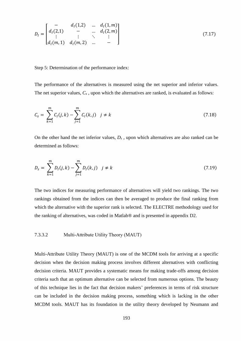
193

𝐷𝐼 = [

− 𝑑𝐼(1,2) … 𝑑𝐼(1,𝑚)𝑑𝐼(2,1) − … 𝑑𝐼(2,𝑚)

⋮ ⋮ ⋱ ⋮𝑑𝐼(𝑚, 1) 𝑑𝐼(𝑚, 2) … −

] (7.17)

Step 5: Determination of the performance index:

The performance of the alternatives is measured using the net superior and inferior values.

The net superior values, Cs , upon which the alternatives are ranked, is evaluated as follows:

𝐶𝑠 = ∑ 𝐶𝐼(𝑗, 𝑘) −

𝑚

𝑘=1

∑ 𝐶𝐼(𝑘, 𝑗)

𝑚

𝑗=1

𝑗 ≠ 𝑘 (7.18)

On the other hand the net inferior values, Ds , upon which alternatives are also ranked can be

determined as follows:

𝐷𝑠 = ∑ 𝐷𝐼(𝑗, 𝑘) −

𝑚

𝑘=1

∑𝐷𝐼(𝑘, 𝑗)

𝑚

𝑗=1

𝑗 ≠ 𝑘 (7.19)

The two indices for measuring performance of alternatives will yield two rankings. The two

rankings obtained from the indices can then be averaged to produce the final ranking from

which the alternative with the superior rank is selected. The ELECTRE methodology used for

the ranking of alternatives, was coded in Matlab® and is presented in appendix D2.

7.3.3.2 Multi-Attribute Utility Theory (MAUT)

Multi-Attribute Utility Theory (MAUT) is one of the MCDM tools for arriving at a specific

decision when the decision making process involves different alternatives with conflicting

decision criteria. MAUT provides a systematic means for making trade-offs among decision

criteria such that an optimum alternative can be selected from numerous options. The beauty

of this technique lies in the fact that decision makers’ preferences in terms of risk structure

can be included in the decision making process, something which is lacking in the other

MCDM tools. MAUT has its foundation in the utility theory developed by Neumann and

194

Morgenstern (Neumann and Morgenstern, 1947) and the elicitation and specific assessment

techniques developed by Keeney and Raiffa (Keeney and Raiffa, 1976). With the combination

of these techniques, the decision criteria of the decision problem can be represented as

individual utility functions which are then aggregated into a single analytical function. The

MAUT method has been applied in solving different multi-criteria decision problems in

different industries. Hwang (2004) utilised MAUT to establish an optimal scenario that can

reduce residents’ exposure to radioactive substances during the elementary phase of a nuclear

power plant accident. Brito and de Almeida (2009) used MAUT to prioritise the risk of

leakage in a natural gas pipeline. The technique was also applied by De Almeida and Bohoris

(1996) in a maintenance strategy selection problem. Having been applied in solving other

problems, the method is used in this thesis to model the maintenance inspection problem

within the marine environment.

The methodological procedure of the MAUT technique is as follows:

Step 1: Formation of the decision problem: The overall aim is to determine the optimal

alternative with respect to some decision criteria. The decision problem is generally

represented in the form of a matrix, an example is shown in Table 7.1. From Table 7.1, the

decision criteria are represented as Bi and the alternatives represented as Aj where i is the

number of decision criteria and j is the number of alternatives. In this particular decision

problem, i is 3 that is to say the decision problem has three decision criteria which are D(T),

C(T) and R(T) and xij are the elements of the decision matrix which are the values evaluated

for alternatives against the decision criteria. The alternatives referred to here are the

inspection intervals, the most appropriate of which is to be determined by the decision maker

(maintenance practitioner) with respect to the decision criteria; D(T), C(T) and R(T). It is the

duty of the decision maker, based on experience and maintenance and failure records of the

marine machinery system, to determine alternative inspection intervals (Aj) for the marine

machinery system which can be rated in hours, days, weeks, months, etc.

Step 2: Determination of single utility functions: The utility function is used to embed the

decision maker’s risk preference in the decision making process. For the different decision

criteria, utility functions are determined which are then applied to form a multi-attribute

utility function. The risk perceptions of the decision maker are of three types which are

incorporated into the utility function. The three risk perceptions are; risk prone, risk neutral

195

and risk averse. The three risk perceptions with respect to the utility function are illustrated in

Figure 7.3.

Figure 7.3: Utility function characteristics (Anders and Vaccaro, 2011)

One popular utility function to define decision criteria is the power series function, as follows

(Anders and Vaccaro, 2011):

𝑢(𝐵𝑖) =(𝐵𝑖 − 𝑎)𝑆

(𝑏 − 𝑎)𝑆 (7.20)

Where S is used to define the risk perception of the decision maker. For a risk-neutral decision

maker, S is given the value of 1 and for risk prone and risk averse decision makers the value

of greater and less than 1 are assigned to S respectively. The maximum and minimum values

of the element of decision criterion Bi are a and b respectively in Eq. 7.20. The outputs of the

utility function of decision criteria range from 0 to 1. In this research it was assumed that the

decision maker was risk neutral and as such the utility function of the three decision criteria;

cost, downtime and reputation are as presented in Eq. 7.21, 7.22 and 7.23 respectively:

𝑢(𝐶(𝑇)) =𝑥1𝑗 − 𝑎1

𝑏1 − 𝑎1 (7.21)

𝑢(𝐷(𝑇)) =𝑥2𝑗 − 𝑎2

𝑏2 − 𝑎2 (7.22)

𝑢(𝑅(𝑇)) =𝑥3𝑗 − 𝑎3

𝑏3 − 𝑎3 (7.23)

196

The constants a1, b1 are the maximum and minimum values of x1j , where x1j are the elements

that belong to the decision criterion cost in the decision matrix in Table 7.1. The constants a2,

b2 are the maximum and minimum values of x2j where x2j are the elements that belong to the

decision criterion downtime. Finally, 𝑏3, 𝑎3 represent the maximum and minimum values of

𝑥3𝑗 where 𝑥3𝑗 are the elements in the decision matrix that belong to the decision criterion

reputation.

Although it was assumed in this research that S was equal to 1, analysis was also conducted

for the situation where S was greater than 1 and less than 1 in order to see the effects it would

have in the decision making process. This was performed as a sensitivity analysis by applying

S in the range of 0 to 2.

Step 3: Determination of multi-attribute utility functions: The individual decision criteria

utility functions determined in step 2, together with their respective scaling constants were

multiplied and then aggregated using either the additive or the multiplicative technique. In

this research the additive technique was utilised and is shown as follows:

𝑈(𝐶(𝑇),𝐷(𝑇), 𝑅(𝑇)) = 𝑤𝑐𝑢(𝐶(𝑇)) + 𝑤𝑑𝑢(𝐷(𝑇)) + 𝑤𝑅𝑢(𝑅(𝑇)) (7.24)

Where 𝑤𝑐, 𝑤𝑑 and 𝑤𝑅 are the scaling constants of the utility functions of decision criteria;

cost, downtime and reputation respectively as determined using the AHP method detailed in

Section 5.3.2.

7.4 Case study 1: Marine diesel engine-sea water cooling pump

The sea water cooling pump is used as a case study in this research to illustrate the

applicability of the proposed integrated MCDM techniques and the delay time model. The sea

water pump is one of the equipment items of the central cooling system of the marine diesel

engine. In Chapters 3 and 4, the FMEA analysis of the entire marine diesel engine was carried

out and from the analysis the sea water pump failure modes were identified as being among

the most critical failure modes of the marine diesel engine. Knowing the risk contribution, the

next step was to define the maintenance strategy to mitigate failures and this was carried out

in Chapter 5. The optimum maintenance strategy for the sea water cooling pump, was

197

identified in Chapter 5 to be offline condition based maintenance (inspection). Finally, in this

chapter, the optimum interval for performing the inspection activities is determined.

7.4.1 Data collection

The basic data needed as input into D(T), C(T) and R(T) in order to determine the optimum

inspection interval for the sea water cooling pump are delay time parameters, cost parameters

and reputation parameters.

Central to the delay time analysis is the delay time distribution and this is generally

determined using two techniques; the subjective and the objective methods. The objective

method usually requires the use of large amounts of equipment failure data in determining

delay time distributions but these are not available in most cases. The use of the subjective

method on the other hand requires limited data but a lot of time is involved in developing

questionnaires and obtaining the required information for estimating delay time (hf) from

experts. For this research, due to difficulty in defining the exact delay time distribution

function, a Weibull distribution was assumed. The Weibull distribution was assumed because

of its flexibility in representing different failures patterns (Krishnasamy et al., 2005, Wang et

al., 2012). Having assumed the Weibull distribution, the delay time probability density

function, f(hf), parameters need to be determined. Due to the unavailability of data to estimate

these parameters, one of the combinations of shape and scale parameters which had

previously been applied by Cunningham et al. (2011) for a sea water cooling pump was used

in this study. The different combinations of shape and scale parameters are presented in Table

7.2. The combination of lower 𝛽 and higher ∅ produces a more definite minimum point in a

delay time model plot (Cunningham et al., 2011). On this basis a combination of 10 and 5

were chosen from Table7.2 for this research.

Table 7.2: Weibull parameters

198

The possible alternative time intervals for inspection of the equipment were determined by

considering the failure data of the equipment, maintenance manuals and with the aid of an

expert with several years of marine diesel engine maintenance experience.

The arrival rate of defects is another variable that needs to be evaluated in the DTA. The

arrival rate of defects and failure rate of equipment items or components are identical if the

equipment items or components are maintained based on reactive maintenance (Cunningham

et al., 2011). In this study, the failure rates in OREDA (2002) were assumed to have been

collected based on reactive maintenance of a system. Based on this assumption, the failure

rates in OREDA 2002 for a centrifugal pump were used as the arrival rate of defects. From

the OREDA 2002 data handbook, the failure rate for the centrifugal pump is given as 1277

per 106 hours for all failure modes.

Having obtained the arrival rate of defects, the next important variables that needed to be

determined were downtimes due to breakdown repair and inspection. For both variables, the

data already available in the literature was relied upon. Cunningham et al. (2011) had taken

downtime due to inspection to be 12.5 minutes. In arriving at 12.5 minutes for downtime due

to inspection of a centrifugal pump of the main cooling system of a passenger ferry, the

authors considered the time used for visual inspection of suction and discharge pressure,

observation of abnormal noise using audio inspection and monitoring of the level of current

drawn by the electric motor by means of electrical inspection. The value of 168 hours for the

downtime as a result of breakdown repair was obtained from OREDA 2002. This value

included the delay in procuring and transporting spare parts.

The three basic cost parameters are cost of inspection (cic), cost of inspection repair (cii) and

cost of breakdown repair (cbr). However cost information was not generally available hence a

combination of experts’ opinions and logged records were relied on to find reasonable

estimates. These estimates were used as input into Eq. 7.7, 7.9 and 7.10 to obtain estimated

values of cost of breakdown repair, cost of inspection repair and cost of inspection

respectively. The estimated costs generated from the equations are presented as follows:

Cost of breakdown repair (cbr) = £52,500

Cost of inspection repair (cii) = £10,500

Cost of inspection (cic) = £210

199

Finally, for the reputation per unit time of the inspection model, two parameters were needed

as input into the model. The two, Rbr and Rii were estimated by experts using an ordinal scale

of 1 to 10. The value assigned was a function of the severity and the occurrence of the failure.

In this research, the worst case scenario was assumed for Rbr since breakdown repair may

sometimes result in catastrophic damage that may affect personnel on a board ship, marine

machinery system equipment and the environment. For Rii, the best case scenario was

assumed since failures are preventatively mitigated. On this basis the values of 1 and 10 were

assigned for Rii and Rbr respectively.

7.4.2 Delay time model analysis

The data for the variables of the delay time models were input into Eq. 7.4, 7.5 and 7.6 to

evaluate downtime per unit cost, cost per unit time and reputation per unit time for different

inspection intervals. The evaluation of Eq. 7.4, 7.5 and 7.6 was achieved using a Matlab

programme as presented in Appendix D1. The results obtained for downtime, cost and

reputation are presented in Figures 7.4, 7.5 and 7.6 respectively.

Figure 7.4: Alternative inspection interval vs downtime per unit time

0 5 10 15 20 25 30 35 40 45 500.02

0.04

0.06

0.08

0.1

0.12

0.14

0.16

0.18

Inspection interval (T(hrs))

D(T

) hrs

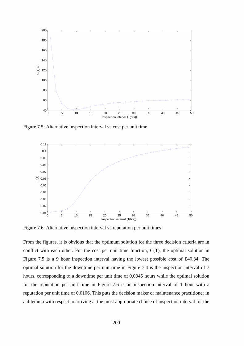
200

Figure 7.5: Alternative inspection interval vs cost per unit time

Figure 7.6: Alternative inspection interval vs reputation per unit times

From the figures, it is obvious that the optimum solution for the three decision criteria are in

conflict with each other. For the cost per unit time function, C(T), the optimal solution in

Figure 7.5 is a 9 hour inspection interval having the lowest possible cost of £40.34. The

optimal solution for the downtime per unit time in Figure 7.4 is the inspection interval of 7

hours, corresponding to a downtime per unit time of 0.0345 hours while the optimal solution

for the reputation per unit time in Figure 7.6 is an inspection interval of 1 hour with a

reputation per unit time of 0.0106. This puts the decision maker or maintenance practitioner in

a dilemma with respect to arriving at the most appropriate choice of inspection interval for the

0 5 10 15 20 25 30 35 40 45 5040

60

80

100

120

140

160

180

200

Inspection interval (T(hrs))

C(T

) £

0 5 10 15 20 25 30 35 40 45 500.01

0.02

0.03

0.04

0.05

0.06

0.07

0.08

0.09

0.1

0.11

Inspection interval (T(hrs))

R(T

)

201

cooling water pump. In such a situation, a multi-criteria technique is needed to aid the

decision maker in reaching a compromise solution.

7.4.3 Formation of decision matrix using D(T), C(T) and R(T) analysis result

In applying the multi-criteria techniques, the first step is to form a decision matrix. The results

of the three decision criteria, D(T), C(T) and R(T) were utilised to produce a decision matrix

which is shown in Table 7.3.

Table 7.3: decision matrix

7.4.4 Determination of Decision criteria weights using AHP

Applying the AHP techniques discussed in Chapter 4, the weights of the decision criteria,

C(T), D(T) and R(T) were obtained as 0.45, 0.3 and 0.25 respectively. AHP is a subjective

method for determining the decision criteria weights and the weights determined using the

technique may vary from expert to expert. Hence there is a need to determine the impact that

varying decision criteria weights may have on the overall ranking of alternative inspection

intervals. The above weights are referred to as case ‘1’. Four other scenarios were used to

202

perform the sensitivity analysis of decision criteria weights. The five scenarios are shown in

Table 7.4. Note: Cases 2 to 4 were used to demonstrate what happens if experts give extreme

values of weights.

Table 7.4: Decision criteria weight cases

7.4.5 Ranking of alternative inspection intervals

7.4.5.1 ELECTRE method ranking

In utilising the ELECTRE method to determine the optimal inspection interval, the decision

matrix in Table 7.3 was normalised using Eq. 7.12 and the result is shown in Table 7.5. The

normalised decision matrix was then multiplied by the weights of the decision criteria (case 1)

to form the weighted normalised matrix, also presented in Table 7.5. This was followed by the

formation of the concordance interval matrix and the discordance interval matrix using Eq.

7.15 and 7.16 respectively. The performance indices, net superior and net inferior values of

each of the inspection intervals were evaluated using Eq. 7.18 and 7.19 and the results are

shown in Table 7.6. Finally, the inspection intervals were ranked based on their net superior

and inferior values and the results are also shown in Table 7.6. The graphical representation of

the net superior values of the inspection intervals and corresponding rankings is presented in

Figure 7.7 while the net inferior values of inspection intervals and corresponding rankings are

shown in Figure 7.8. The performance of the inspection interval can be determined by

applying the net superior index; in this case, the inspection interval with the highest superior

value is selected as the most appropriate. The performance of the inspection intervals can also

be determined using the net inferior index and in this case the inspection interval with the

lowest net inferior value is selected as the optimal solution.

From the net superior performance index in Figure 7.7 an inspection interval of 9 hours is the

best ranked having the highest net superior value of 21.40 and as such, based on this

performance index, it is the most appropriate interval for the inspection of the cooling water

203

pump. The worst solution is the inspection interval of 49 hours which has the lowest net

superior value of -22.20.

From Figure 7.8 an inspection interval of 9 hours is the optimal solution to this inspection

interval selection problem having the lowest net inferior value of -31.3334. The second

ranked inspection interval is 7 hours with a net inferior value of -28.7606 while the lowest

ranked inspection interval is 49 hours with a net inferior value 32.7569. The inspection

interval of 7 hours might also be recommended because of the closeness of its net inferior

value to that of the 9 hour inspection interval.

Table 7.5: Normalised and weighted normalised matrix

204

Table 7.6: ELECTRE II ranking of inspection interval

Figure 7.7: Net superior values and corresponding ranks of inspection interval

0

5

10

15

20

25

30

-25.0000

-20.0000

-15.0000

-10.0000

-5.0000

0.0000

5.0000

10.0000

15.0000

20.0000

25.0000

1 3 5 7 9 11 13 15 17 19 21 23 25 27 29 31 33 35 37 39 41 43 45 47 49 Ran

k

Net

su

per

ior-

Cs

Inspection interval-T(hrs)

Net superior (Cs) Rank

205

Figure 7.8: Net inferior (Ds) values and corresponding ranks of inspection intervals

Sensitivity analysis

One of the variables that affects the ranking of alternative inspection intervals produced by

the ELECTRE method is the decision criteria weight. In this study, AHP was used to

determine decision criteria weights. The technique is highly subjective and as such different

experts or decision makers might assign different weights to each decision criterion. In order

to study the effects of varying weights that may be assigned by the decision makers on the

rankings of inspection intervals obtained from the ELECTRE method, a sensitivity analysis

was performed using various combinations of decision criteria weight. The various

combinations of decision criteria weights applied for the sensitivity analysis study are

presented in Table 7.4. From the sensitivity analysis study, the performance indices net

superior and net inferior values obtained for alternative inspection intervals in the five

different combinations of decision criteria weights (cases 1-5) are presented in Figures 7.9

and 7.10 and in tabular format in Tables D4 and D5 in Appendix D4. The corresponding

rankings of inspection interval based on the net superior and net inferior values are presented

in Figures 7.11 and 7.12 respectively and in tabular form in Tables D6 and D7 respectively in

Appendix D4.

0

5

10

15

20

25

30

-40.0000

-30.0000

-20.0000

-10.0000

0.0000

10.0000

20.0000

30.0000

40.0000

1 3 5 7 9 11 13 15 17 19 21 23 25 27 29 31 33 35 37 39 41 43 45 47 49 Ran

k

Net

infe

rio

r-D

s

inspection interval-T(hrs)

Net inferior (Ds) Rank

206

Figure 7.9: Net superior-Cs values from decision criteria weight sensitivity analysis

Figure 7.10: Net inferior-Ds values from decision criteria weight sensitivity analysis

-30.0000

-20.0000

-10.0000

0.0000

10.0000

20.0000

30.0000

1 3 5 7 9 11 13 15 17 19 21 23 25 27 29 31 33 35 37 39 41 43 45 47 49

Net

su

per

ior-

Cs

Inspection interval-T(hrs)

Case1 Case2 Case3 Case4 Case5

-40.0000

-30.0000

-20.0000

-10.0000

0.0000

10.0000

20.0000

30.0000

40.0000

1 3 5 7 9 11 13 15 17 19 21 23 25 27 29 31 33 35 37 39 41 43 45 47 49

Net

infe

rio

r-D

s

Inspection interval-T(hrs)

Case1 Case2 Case3 Case4 Case5

207

Figure 7.11: Net superior-Cs rankings from decision criteria weight sensitivity analysis

Figure 7.12: Net inferior-Ds rankings from decision criteria weight sensitivity analysis

From the result of the net superior performances of the alternative inspection intervals in

Figure 7.9 and the corresponding rankings in Figure 7.11, the optimal inspection interval for

the five cases varies from 7 hours to 9 hours. The optimal inspection interval for the five cases

based on the net superior index is presented in Table 7.7. The optimal inspection interval for

0

5

10

15

20

25

30

1 2 3 4 5 6 7 8 9 10 11 12 13 14 15 16 17 18 19 20 21 22 23 24 25

Net

su

per

ior-

Cs-

Ran

kin

g

Inspection-T(hrs)

Case1 Case2 Case3 Case4 Case5

0

5

10

15

20

25

30

1 2 3 4 5 6 7 8 9 10 11 12 13 14 15 16 17 18 19 20 21 22 23 24 25

Net

infe

rio

r-D

s R

ank

Inspection interval-T(hrs)

Case1 Case2 Case3 Case4 Case5

208

the five cases based on net inferior index in Figure 7.10 and the corresponding ranking of

inspection intervals in Figure 12 also vary from 7 hours to 9 hours. The optimal inspection

interval for the five cases based on the net inferior index are tabulated in Table 7.8.

Table 7.7: Optimal inspection interval for five cases

Table 7.8: Optimal inspection interval for five cases

7.4.5.2 MAUT method rankings

The MAUT technique used in the ranking of inspection intervals commenced with the

formation of the decision matrix shown in Table 7.3. The first step to solving the decision

matrix in Table 7.3 using the MAUT method was to define the range of each decision

criterion, the results of which are shown in Table 7.9. The values in Table 7.9 were then used

as inputs into Eq. 7.21 to 7.23 to calculate the utility values of each alternative inspection

interval against the decision criteria. Finally, the multi-attribute function values of each

inspection interval were evaluated by aggregating utility values of the alternative inspection

intervals multiplied by decision criteria weights as expressed in Eq. 7.24. The multi-attribute

function values of each of the inspection intervals obtained using Eq. 7.24 are shown in Table

7.10 and Figure 7.13.

209

Table 7.9: Range of decision criteria

Table 7.10: MAUT ranking

210

Figure 7.13: Multi-attribute utility function U(C(T), D(T), R(T)) based on inspection intervals

From Table 7.10 and Figure 7.13, an inspection interval of 7 hours is in the first position

having the highest multi-attribute utility function value of 0.9927 and as such it is the

optimum solution for the inspection interval selection problem. The inspection interval in

second position is 9 hours, having multi-attribute utility function value of 0.9556. The

inspection interval in last position is 49 hours, having the lowest multi-attribute function value

i.e. 0.0857.

Sensitivity analysis

The results obtained above using the MAUT technique are when the decision maker is risk

neutral, in which case R is equal to 1. However there are situations where the decision maker

may be risk prone or risk averse and in such situations R is greater than 1 (risk prone) or less

than 1 (risk averse). The effect of the risk perception of the decision maker was investigated

to see how it would affect the rankings of the inspection interval. Based on this a range of R

from 0 to 2 was used and the results obtained are shown in Figure 7.14 and Table D1 in

Appendix D4.

0

5

10

15

20

25

30

0.0000

0.2000

0.4000

0.6000

0.8000

1.0000

1.2000

1 3 5 7 9 11 13 15 17 19 21 23 25 27 29 31 33 35 37 39 41 43 45 47 49

Ran

k

U(C

(T),

D(T

),R

(T))

Inspection interval-T(hrs)

U(C(T),D(T),R(T) Rank

211

Figure 7.14: Sensitivity analysis of R

From Figure 7.14, the inspection interval of 7 hours has the maximum multi-attribute utility

function value when R=0.5, 1, 1.5 and 2. From this it obvious that the result produced when

the decision maker is risk averse, neutral and risk prone is the same. From the graph it is

obvious that when R is assigned with the value of zero, no reasonable result can be produced

i.e. the alternative inspection intervals cannot be prioritised. In a case in the literature (see the

work of Anders and Vaccaro, 2011) it was shown that there was difference in the result

produced when the decision maker is risk-averse but with no distinction between results

produces by risk-neutral and risk prone persons however in the present work the result was

same for all categories of decision maker.

Another factor that has strong influence on the outcome of the MAUT analysis is the weight

of the decision criteria. The data in Table 7.4 was used as input data into the MAUT method

in performing the sensitivity analysis of decision criteria weights. This was done to determine

the effects of varying weights of decision criteria on the output of the MAUT method. The

multi-attribute utility function values obtained from the five cases and the corresponding

rankings of the inspection intervals are presented in Figures 7.15 and 7.16 and in Tables D2

and D3 in Appendix D4. From Figure 7.15, the inspection interval of 7 hours has the highest

value of multi-attribute utility function value for the five cases and as such was ranked 1 in

Figure 7.16. For the optimal inspection interval to have remained the same for the five cases

shows that the MAUT technique is very robust and less sensitive to decision criteria weight

changes.

0

0.2

0.4

0.6

0.8

1

1.2

1 3 5 7 9 11 13 15 17 19 21 23 25 27 29 31 33 35 37 39 41 43 45 47 49

U(C

(T),

D(T

),R

(T))

Inspection interval-T(hrs)

R=0 R=0.5 R=1 R=1.5 R=2

212

Figure 7.15: Multi-attribute utility function values for varying weights of decision criteria

Figure 7.16: Inspection intervals rank for varying weights of decision criteria

7.4.6 Comparison of MAUT and ELECTRE ranking methods

The rankings of the inspection interval alternatives produced by the two methods are shown in

Table 7.11 and Figure 7.17. From Figure 7.17 it is obvious that the two techniques,

ELECTRE and MAUT yield very similar results. The rankings produced from the two

0.0000

0.2000

0.4000

0.6000

0.8000

1.0000

1.2000

1 3 5 7 9 11 13 15 17 19 21 23 25 27 29 31 33 35 37 39 41 43 45 47 49

U(C

(T),

D(T

),R

(T))

Inspection interval-T(hrs)

Case1 Case2 Case3 Case4 Case5

0

5

10

15

20

25

30

1 3 5 7 9 11 13 15 17 19 21 23 25 27 29 31 33 35 37 39 41 43 45 47 49

Ran

k

Inspection-T(hrs)

Case1 Case2 Case3 Case4 Case5

213

ELECTRE ranking indices, the net superior (represented in the graph as ELECTRE (Cs)) and

the net inferior (represented in the graph as ELECTRE (Ds)) are the same for most of the

inspection intervals with only a few having a rank difference of one between them. When the

results of the two ranking indices of ELECTRE are also compared with the result generated

from the MAUT method, the results are also very similar. To further show the relationship

between the three ranking systems, a Spearman rank correlation test was performed. The

Spearman correlation coefficients obtained between ELECTRE (Cs) and ELECTRE (Ds),

between MAUT and ELECTRE (Cs) and between MAUT and ELECTRE (Ds) are 0.928,

0.998 and 0.906 respectively. The near perfect correlation obtained among the three ranking

methods revealed that they can be applied individually to rank alternative inspection intervals

for marine machinery systems so that the optimal solution can be obtained. The optimal

solution obtained for the water cooling pump from ELECTRE (Cs) and ELECTRE (Ds) was

an inspection interval of 9 hours and for the MAUT technique is 7 hours. The two techniques

can also be compared in terms of robustness. From the results of the five cases in the

sensitivity analysis of decision criteria weights, the MAUT method gave the same optimal

solution in all cases while the ELECTRE method had an optimal solution that varied from 7

hours to 9 hours. This shows that the MAUT technique is more robust and less sensitive to

decision criteria weight changes than the ELECTRE method. The MAUT method is therefore

recommended for the marine industry for determining optimal inspection intervals.

214

Table 7.11: Comparison of methods

Figure 7.17: Comparative ranking of alternative inspection intervals

7.5 Summary

In monitoring the condition of an asset, the two options are continuous condition monitoring

and periodic condition monitoring. The periodic monitoring approach is commonly used

because it is more cost effective than the continuous condition monitoring approach. However

the major challenge of the periodic condition monitoring technique is the determination of the

123456789

101112131415161718192021222324252627

1 3 5 7 9 11 13 15 17 19 21 23 25 27 29 31 33 35 37 39 41 43 45 47 49

Ran

ks

Inspection intervals-T(hrs)

Electre(Ds)

Electre(Cs)

MAUT

215

most appropriate interval for performing inspection. Traditionally, maintenance practitioners

rely on their experience in determining the most appropriate time for carrying out inspection

activities. The delay time approach has been reported in the literature, however in determining

the optimal inspection interval most of the authors applied a single decision criterion (cost or

downtime). The purpose of this research was to apply multiple decision criteria in obtaining

the optimal inspection interval. Three decision criteria; cost, downtime and reputation were

chosen for measuring performance of an inspection interval.

The delay time concept was used to model the relationship between inspection intervals and

the corresponding cost, downtime and reputation due to system failure. Since the optimal

solutions obtained from the three decision criteria are in conflict with each other, the three

decision criteria results were aggregated with two MCDM techniques; MAUT and

ELECTRE. To illustrate the applicability of the proposed methodology for determining an

optimal inspection interval, a case study of a sea water cooling pump was investigated. From

the analysis, the rankings of alternative inspection intervals produced from both the MAUT

and ELECTRE methods were very similar. To further prove the similarity between the two

MCDM techniques, the Spearman rank correlation coefficient between the techniques was

evaluated and showed a near perfect relationship. This confirms that the two techniques can

be applied individually or in combination to rank and select the best inspection policy for

marine machinery systems.

The robustness of the two methods; MAUT and ELECTRE was tested via sensitivity analysis

of the decision criteria weight. The five different combinations of decision criteria weights

chosen for the sensitivity analysis revealed that the MAUT method is more robust and less

sensitive to decision criteria weight variations. The preference of the decision maker for

decision criteria weightings was accommodated through use of AHP which can both

quantitatively and qualitatively determine the weight of decision criteria. Despite the

suitability of both techniques for optimal inspection interval determination, the MAUT

method was recommended for the marine machinery system for the following reasons:

(1) The risk preference of maintenance practitioners is accommodated in the MAUT

method which is not something that is available in the ELECTRE method and

(2) The MAUT method is more robust, as evidenced by the sensitivity analysis of the

decision criteria weight.

216

In this study, the MAUT and ELECTRE methods have been validated for inspection selection

problems within the framework of marine machinery systems however they could also be

applied in solving inspection selection problems for other related engineering systems.

217

Chapter 8 Conclusions, Contributions and Recommendation for future

work

8.1 Conclusions

Ship systems will not remain safe and reliable no matter how well designed and manufactured

they are if they are not properly maintained. However over-maintenance may result in system

degradation and excessive costs that may lead to increases in the operational cost of the

system. On the other hand, under-maintenance may result in system failures that may be

catastrophic. Hence there is a need for a sound and effective system to be in place for the

maintenance of ship systems such that their availability and cost of maintenance are

optimised. Basically, there are three key elements of a maintenance system which are; risk

assessment, maintenance strategy selection and maintenance task interval determination.

RCM is one of the more commonly used methods for the optimisation of these three key

elements of a maintenance management system. From the extensive literature survey

performed it was obvious that the tools used in the RCM methodology have flaws which limit

the effectiveness of the approach in optimising ship system availability. Hence the main

purpose of this research was to develop alternative tools to enhance the RCM methodology

such that ship systems are more effectively maintained and managed for improved availability

and reduced downtime and at a reasonable cost which will invariably result in a significant

reduction in operational cost. To achieve this aim different methodologies were developed for

risk assessment, maintenance strategy selection and maintenance interval determination.

In the area of risk prioritisation four methods were proposed in this study; an averaging

technique integrated with RPN, averaging technique integrated with VIKOR, averaging

technique integrated with TOPSIS and averaging technique integrated with CP. For the four

proposed techniques, the novel averaging technique was used in aggregating multiple experts’

opinions that may be imprecise, while the RPN, TOPSIS, VIKOR and CP methods were used

in the ranking of the risk of the individual failure modes. The suitability and validity of the

proposed methods were demonstrated with case studies of partial and full marine machinery

systems and case studies from the literature. The results showed that the four proposed

methods are strongly correlated and can individually be applied for risk prioritisation more

efficiently than the classical FMEA and other approaches in literature.

218

In the area of maintenance strategy selection three hybrid MCDM maintenance strategy

selection methods were proposed: (1) Delphi-AHP (2) Delphi-AHP-PROMETHEE and

(3) Delphi-AHP-TOPSIS. From the analysis of the results, the three proposed

methodologies yielded the same optimum solution for the cooling water pump of the

marine diesel engine for both; the single expert decision making process and the group

decision making process. Based on the information that was obtained from the experts, the

decision criterion ‘safety’, was found to be the driving force for the selection of the

maintenance strategy. The scheduled on-condition task or OFCBM, which was the

optimum solution for maintaining the cooling water pump of the diesel engine in both

scenarios, was in-line with the current best practice in the marine industry. The proposed

methods avoid the limitations of RCM logic tree analysis which has an inability to rank

alternative maintenance strategies and they are also less computationally intensive than

approaches in the literature.

In the area of maintenance task interval determination two of the five maintenance task

options utilised in maintenance management were modelled. The maintenance tasks

considered were; (1) scheduled replacement and (2) scheduled on-condition task.

o For the scheduled replacement interval determination age replacement models

were integrated with TOPSIS. While the ARM were used in modelling decision

criteria, TOPSIS was applied in aggregating decision criteria and in the ranking of

alternative replacement intervals. From the results of the analysis it can be

concluded that the proposed methodology is both simple and robust. The approach

has the advantage of including criteria weighting with both objective and

subjective components whereas most previous research only included subjective

components.

o For the inspection interval determination two MCDM tools; MAUT and

ELECTRE were combined with the delay time model. The suitability of the

integrated delay time and the MCDM model was demonstrated with a case study

of a cooling water pump of a marine diesel engine. From the results both the

MAUT and the ELECTRE methods produced the same optimal inspection interval

for the cooling water pump. The proposed approaches have the advantage of

simultaneously using multiple decision criteria in determining optimum inspection

interval as opposed to current approaches in literature that use a single criterion.

219

In these proposed methodologies seven different MCDM tools: VIKOR, CP, TOPSIS, AHP,

PROMETHEE, MAUT and ELECTRE were used for the ranking of alternatives in the areas

of risk assessment, maintenance strategy selection and maintenance interval determination.

However each of these tools has the capability to rank alternatives in all three elements of the

maintenance system. Their individual use will depend on the practitioners’ and/or analysts’

choice which may be guided by ease of implementation (computational effort) and suitability

(Løken, 2007). To guide the practitioner with respect to making a choice on the basis of ease

of implementation Table 8.1 is presented below. From the table there are two categories of

MCDM tools based on the different criteria such as Hand calculation in measuring ease of

implementation; those that are easy to implement such as CP and MAUT with or without

software and those that are difficult to implement without software such as ELECTRE and

PROMETHEE.

Table 8.1: Degree of ease of implementation of MCDM tools

Computational

effort

MCDM tools

TOPSIS VIKOR CP AHP ELECTRE MAUT PROMETHEE

Hand calculation × × × × ×

Spreadsheet × ×

Software tool × × ×

Software code × ×

Hand calculation/spreadsheet: Tick- easy to calculate using hand calculation/spreadsheet & Cross-difficult to

calculate using hand calculation/spreadsheet

Software tool: Tick- software available & Cross-software not available

Software code: Tick- easy to code & Cross- difficult to code

The work demonstrated is an enhanced RCM system and in reality RCM methodologies are

already routine for whole ship maintenance and as such the proposed enhance RCM does not

need scaling up to make it applicable to entire ship maintenance. Concerning the practicality

of a shipping company implementing the proposed enhanced RCM methodology, this will

generally require a team which should consist of both external and internal experts, technical

managers, superintended engineers and chief engineers and a statistician who will be able to

identify appropriate functions such as the Weillbull distribution. Once the expert team has

implemented the enhanced RCM methodology it would be straightforward for practitioners

on board to utilise.

220

8.2 Research Contribution

This research presents the development of various tools in order to support the RCM

methodology and to improve its effectiveness in marine maintenance system applications.

This will result in an improvement in marine system reliability at minimum cost. The

contribution of this research has been disseminated through journal and conference

publications listed in the publication section. In particular the research contributions with

regard to addressing the limitations of RCM in the optimisation of the three major elements of

maintenance management are as follows:

(1) Development of a methodology for the assessment of the risk of marine machinery

systems. The innovation of this risk assessment methodology is in the combination of

different MCDM tools such as VIKOR, CP, and TOPSIS in addressing the limitations of

classical FMEA that is frequently used within the framework of RCM in the risk assessment

of marine systems. Although VIKOR, CP and TOPSIS have been applied individually by

practitioners in solving other multi-criteria decision problems they have not been used in

solving the fundamental risk prioritization problem. The incorporation of the averaging

technique into the approaches further makes the methodology unique as it allows for the use

of both precise and imprecise ratings provided by experts to be applied as input into VIKOR,

CP and TOPSIS which each normally use only precise data, thereby providing a more

efficient technique for risk prioritization that is highly beneficial to the marine industry. An

additional important feature of this proposed methodology is in the breakaway from the use of

a subjective weighting technique, such as AHP, in assigning decision criteria weights, by also

integrating the variance and entropy methods into VIKOR, CP and TOPSIS.

(2) Development of a methodology for maintenance strategy selection based on the

integration of the RCM concept with multi-criteria decision making methods. The novelty in

the proposed methodology lies in the combination of different MCDM tools such as AHP,

PROMETHEE and TOPSIS for solving the problem of maintenance strategy selection within

the framework of marine system maintenance. Another important feature of the proposed

methodology is the incorporation of the Delphi method into AHP, PROMETHEE and

TOPSIS. The Delphi method was introduced in order to collect, identify and screen decision

criteria such that the most important decision criteria are applied in selecting the optimal

maintenance strategy for the marine system.

221

(3) Development of a methodology for the determination of the optimal interval for

scheduled replacement. The innovation of the methodology is based on the integration of the

Age Replacement Model (ARM) with the TOPSIS technique which has never been used

before for preventive replacement interval determination in the maritime environment.

Another important feature of the proposed methodology is the combination of an efficient

decision criteria weighting framework into the ARM and TOPSIS models. The efficient

decision criteria weighting framework integrates both subjective and objective techniques in

evaluating the weights of decision criteria, as opposed to the use of only a subjective

technique for land based system applications found in literature. The weighting framework is

so flexible that it allows maintenance practitioners to either use a subjective criteria weighting

technique or an objective weighting technique or a combination of both techniques.

(4) Development of a methodology for the determination of the optimal interval for

scheduled inspection. The novelty again lies in the combination of MCDM tools (MAUT and

ELECTRE methods) with a delay time model in determining the optimum intervals for

performing inspections for systems for the first time within the maritime maintenance

framework. Another important feature of the methodology is the use of the delay time concept

in the development of a company reputation model. The company reputation is used as a

decision criterion in addition to already established cost and downtime decision criteria delay

time models in determining inspection intervals for maintaining plant system equipment.

8.3 Limitations encountered

One of the greatest challenges that was encountered in the execution of this study was the

problem of real life data availability. The lack of reliable real life data in terms of both

quantity and quality in most scenarios was the reason behind the use of experts’ opinions and

data from literature as alternatives in this research.

8.4 Recommendation for future work

8.4.1 Risk assessment

The technique that was applied in this study for risk assessment, FMEA, is a well-established

qualitative technique which is useful in making maintenance decisions. However a

quantitative approach is more reliable in making such decisions. On this basis, a quantitative

approach such as FTA may be exploited in determining risk of failure modes of marine

222

machinery systems. Furthermore, in this study the FMEA that was performed on the marine

diesel engine, could be extended to the whole ship system. In addition, three MCDM tools;

VIKOR, CP and TOPSIS have been used however other MCDM techniques such as

EXPROM 2 may also be applied in determination of the risk of failure modes of marine

machinery systems.

8.4.2 Maintenance strategy selection

Although the proposed methodologies have been validated for marine machinery system they

can also be applied to other related engineering systems and, depending on the preferences of

the maintenance practitioners, the decision criteria can further be reduced in order to make the

evaluation process easier. Furthermore, other techniques such as the MAUT, VIKOR and

EXPROM 2 may be applied for the ranking of alternative maintenance strategies. There may

also be the need to capture the expert information imprecisely rather than obtaining precise

data from experts. In such a scenario, information from experts would be in the form of an

estimated interval and, in addressing this, the fuzzy logic technique may be integrated within

the proposed methodologies.

8.4.3 Maintenance interval determination

The five maintenance strategies considered in this study are; scheduled overhaul, scheduled

replacement, offline condition based maintenance (inspection) and online condition based

maintenance. From these five maintenance strategies, methodologies have been developed for

determining the optimum interval for carrying out offline condition based maintenance and

scheduled replacement (SRP) tasks. For future work a methodology could be developed for

determining the interval for performing scheduled overhaul and scheduled replacement.

8.4.3.1 Scheduled replacement interval determination

The methodology for determining the scheduled replacement interval in this study is based on

a multi-criteria decision framework, the three decision criteria being; cost, downtime and

reliability. The cost and downtime models were adapted from the Barlow and Hunter (1960)

age replacement model. The TOPSIS methodology was applied in simultaneously obtaining

the ranking of alternative replacement intervals for marine machinery systems from the three

decision criteria. For future work other MCDM tools such as MAUT and ANP may be

exploited for the ranking of the alternative replacement intervals such that an optimum

223

solution can be obtained. For example, the MAUT method will allow the maintenance risk

perception to be included in the decision making process which is not possible in the

proposed method in this research and the ANP allowed for the interrelationship between the

decision criteria to be utilised in the analysis process which again is not possible in the

method utilised in this study. For the three decision criteria models the failure distribution of

the systems that were studied were assumed to follow a Weibull distribution, however other

well know distributions such as exponential and normal distributions should be investigated.

Alternatively system failure data could be obtained to determine the exact distribution rather

than assuming it.

8.4.3.2 Inspection interval determination

In determining the intervals for performing the inspection for the system under investigation,

the delay time model was integrated with the multi-criteria decision tools ELECTRE and

MAUT. The delay time was used to model the three decision criteria; cost, downtime and

reputation, while the ranking of alternative inspection intervals was performed using MAUT

and ELECTRE. For the delay time models the Weibull distribution was assumed as the

distribution probability of the delay time. For future work other known distributions such as

exponential and normal distributions could also be studied. A database system should be

developed such that the shipping industry can easily gather delay time information. For the

ranking of alternative inspection intervals the use of other MCDM techniques such as

EXPROM 2 and PROMETHEE can be explored.

224

References

AGHAJANI BAZZAZI, A., OSANLOO, M. & KARIMI, B. 2011. Deriving preference order of open pit mines

equipment through MADM methods: Application of modified VIKOR method. Expert Systems with

Applications, 38, 2550-2556.

AHMAD, R. & KAMARUDDIN, S. 2012. An overview of time-based and condition-based maintenance in

industrial application. Computers & Industrial Engineering, 63, 135-149.

AHMAD, R., KAMARUDDIN, S., AZID, I. & ALMANAR, I. 2011a. Maintenance management decision

model for preventive maintenance strategy on production equipment. J. Ind. Eng. Int, 7, 22-34.

AHMAD, R., KAMARUDDIN, S., AZID, I. A. & ALMANAR, I. P. 2011b. Preventive replacement schedule: a

case study at a processing industry. International Journal of Industrial and Systems Engineering, 8,

386-406.

AHMED, S., HJ. HASSAN, M. & TAHA, Z. 2005. TPM can go beyond maintenance: excerpt from a case

implementation. Journal of Quality in Maintenance Engineering, 11, 19-42.

AHUJA, I. P. S. & KHAMBA, J. S. 2008. Total productive maintenance: literature review and directions.

International Journal of Quality & Reliability Management, 25, 709-756.

AL-FAWZAN, M. A. 2000. Methods for estimating the parameters of the Weibull distribution. King Abdulaziz

City for Science and Technology, Riyadh, Saudi Arabia, 91.

AL-NAJJAR, B. & ALSYOUF, I. 2003. Selecting the most efficient maintenance approach using fuzzy multiple

criteria decision making. International Journal of Production Economics, 84, 85-100.

ALEKSIĆ, M. & STANOJEVIĆ, P. 2007. Reliability centred maintenance. RCM - Održavanje prema

pouzdanosti, 5, 41-45.

ALEXANDER, D. Application of Monte Carlo simulations to system reliability analysis. Proceedings of the

20th International Pump Symposium, Houston, TX, 2003.

ALHOULI, Y., LING, D., KIRKHAM, R. & ELHAG, T. Performance Measurement of Marine Vessel

Maintenance Operations: A Case Study of Kuwaiti Shipping Companies. 5 th Annual Conference

Liverpool “BEAN” 18 th-19 th May 2010, 2010. 26.

ALMEIDA, A. T. 2012. Multicriteria model for selection of preventive maintenance intervals. Quality and

Reliability Engineering International, 28, 585-593.

AMERICAN BUREAU OF SHIPPING. 2000. Guidance notes on risk assessment applications for the marine

and offshore oil and gas industries. [Online]. Houston, USA: American Bureau of shipping.

AMERICAN BUREAU OF SHIPPING 2003. Guide for Survey based on Reliability-Centered maintenance,

Houston, USA, America Bureau of Shipping.

AMERICAN BUREAU OF SHIPPING 2004. Guidance note on Reliability-Centered Maintence. Houston, USA:

American Bureau of Shipping.

ANDERS, G. J. & VACCARO, A. 2011. Innovations in power systems reliability, Springer.

ANOJKUMAR, L., ILANGKUMARAN, M. & SASIREKHA, V. 2014. Comparative analysis of MCDM

methods for pipe material selection in sugar industry. Expert Systems with Applications, 41, 2964-2980.

ARENDT, J. S. 1990. Using quantitative risk assessment in the chemical process industry. Reliability

Engineering and System Safety, 29, 133-149.

225

ARTHUR, N. 2005. Optimization of vibration analysis inspection intervals for an offshore oil and gas water

injection pumping system. Proceedings of the Institution of Mechanical Engineers, Part E: Journal of

Process Mechanical Engineering, 219, 251-259.

ARUNRAJ, N. S. & MAITI, J. 2007. Risk-based maintenance-Techniques and applications. Journal of

Hazardous Materials, 142, 653-661.

ARUNRAJ, N. S. & MAITI, J. 2010. Risk-based maintenance policy selection using AHP and goal

programming. Safety Science, 48, 238-247.

AVEN, T. & JENSEN, U. 1999. Stochastic models in reliability, Springer.

AYADI, D., AZZABI, L., KOBI, A., BACHAR, K. & ROBLEDO, C. 2013. A multicriteria failure mode and

effects analysis approach for optimizing human safety. IEEE Reliability And Maintainability

Symposium (RAMS), January 18-31 2013 Orlando FL. 1-9.

BAHRAMI-G, K., PRICE, J. W. H. & MATHEW, J. 2000. The constant-interval replacement model for

preventive maintenance: A new perspective. International Journal of Quality & Reliability

Management, 17, 822-838.

BARLOW, R. & HUNTER, L. 1960. Optimum preventive maintenance policies. Operations Research, 8, 90-

100.

BEHZADIAN, M., KAZEMZADEH, R. B., ALBADVI, A. & AGHDASI, M. 2010. PROMETHEE: A

comprehensive literature review on methodologies and applications. European Journal of Operational

Research, 200, 198-215.

BEJGER, A. 2011. An analysis of chosen engine failures of the "Seismic Research" type ship. Journal of Polish

CIMAC, 6, 9-14.

BEN-DAYA, M. 2009. Failure Mode and Effect Analysis. Handbook of maintenance management and

engineering. first ed.: Springer.

BENI, S. S. 2014. Implementation of Computerised Maintenance Management System in National Iranian Gas

Company and sub-companies. Proceedings of the 2014 International Conference on Industrial

Engineering and Operations Management Bali, Indonesia, January, 7-9 2014, 1181-1186.

BERTOLINI, M. & BEVILACQUA, M. 2006. A combined goal programming - AHP approach to maintenance

selection problem. Reliability Engineering and System Safety, 91, 839-848.

BEVILACQUA, M. & BRAGLIA, M. 2000. Analytic hierarchy process applied to maintenance strategy

selection. Reliability Engineering and System Safety, 70, 71-83.

BEVILACQUA, M., BRAGLIA, M. & GABBRIELLI, R. 2000. Monte Carlo simulation approach for a

modified FMECA in a power plant. Quality and Reliability Engineering International, 16, 313-324.

BILBAO-TEROL, A., PÉREZ-GLADISH, B. & ANTOMIL-LBIAS, J. 2006. Selecting the optimum portfolio

using fuzzy compromise programming and Sharpe’s single-index model. Applied Mathematics and

Computation, 182, 644-664.

BOLLOJU, N. 2001. Aggregation of analytic hierarchy process models based on similarities in decision makers’

preferences. European Journal of Operational Research, 128, 499-508.

BOWLES, J. B. 1998. New SAE FMECA standard. Jan 19 - 22 1998 Anaheim, CA, USA. 48-53.

BOWLES, J. B. An assessment of RPN prioritization in a failure modes effects and critically analysis. 2003.

380-386.

BRAGLIA, M. 2000. MAFMA: Multi-attribute failure mode analysis. International Journal of Quality and

Reliability Management, 17, 1017-1034.

226

BRAGLIA, M., FROSOLINI, M. & MONTANARI, R. 2003. Fuzzy TOPSIS Approach for Failure Mode,

Effects and Criticality Analysis. Quality and Reliability Engineering International, 19, 425-443.

BRANS, J.-P. 1986. L'élaboration d'instruments d'aide à la décision. Nadeau, Raymond et Maurice Landry, 183-

213.

BRANS, J.-P. & VINCKE, P. 1985. Note—A Preference Ranking Organisation Method: (The PROMETHEE

Method for Multiple Criteria Decision-Making). Management science, 31, 647-656.

BRANS, J. P., VINCKE, P. & MARESCHAL, B. 1986. How to select and how to rank projects: The Promethee

method. European Journal of Operational Research, 24, 228-238.

BRITO, A. J. & DE ALMEIDA, A. T. 2009. Multi-attribute risk assessment for risk ranking of natural gas

pipelines. Reliability Engineering & System Safety, 94, 187-198.

BS/ISO 3811, 1993. Glossary of Terms used in Terotechnology. Common BSI/ISO standard,

London

BS/ISO 17359, 2003. Condition monitoring and diagnostics of machines-General guidelines

Common BS/ISO standard, London

ÇALIŞKAN, H., KURŞUNCU, B., KURBANOĜLU, C. & GÜVEN, T. Y. 2013. Material selection for the tool

holder working under hard milling conditions using different multi criteria decision making methods.

Materials and Design, 45, 473-479.

CAPUTO, A. C., PELAGAGGE, P. M. & SALINI, P. 2013. AHP-based methodology for selecting safety

devices of industrial machinery. Safety Science, 53, 202-218.

CARMIGNANI, G. 2009. An integrated structural framework to cost-based FMECA: The priority-cost FMECA.

Reliability Engineering and System Safety, 94, 861-871.

CARPINELLI, G., CARAMIA, P., MOTTOLA, F. & PROTO, D. 2014. Exponential weighted method and a

compromise programming method for multi-objective operation of plug-in vehicle aggregators in

microgrids. International Journal of Electrical Power & Energy Systems, 56, 374-384.

CARTER, D. A., HIRST, I. L., MADDISON, T. E. & PORTER, S. R. 2003. Appropriate risk assessment

methods for major accident establishments. Process Safety and Environmental Protection: Transactions

of the Institution of Chemical Engineers, Part B, 81, 12-18.

CAVALCANTE, C. A. V. & DE ALMEIDA, A. T. 2007. A multi-criteria decision-aiding model using

PROMETHEE III for preventive maintenance planning under uncertain conditions. Journal of Quality

in Maintenance Engineering, 13, 385-397.

CAVALCANTE, C. A. V., FERREIRA, R. J. P. & DE ALMEIDA, A. T. 2010. A preventive maintenance

decision model based on multicriteria method PROMETHEE II integrated with Bayesian approach.

IMA Journal of Management Mathematics, 21, 333-348.

CAVALLI-SFORZA, V. & ORTOLANO, L. 1984. DELPHI FORECASTS OF LAND USE:

TRANSPORTATION INTERACTIONS. Journal of Transportation Engineering, 110, 324-339.

CHAREONSUK, C., NAGARUR, N. & TABUCANON, M. T. 1997. A multicriteria approach to the selection

of preventive maintenance intervals. International Journal of Production Economics, 49, 55-64.

CHATTERJEE, P., ATHAWALE, V. M. & CHAKRABORTY, S. 2009. Selection of materials using

compromise ranking and outranking methods. Materials & Design, 30, 4043-4053.

CHEN, F. 1997. Issues in the continuous improvement process for preventive maintenance: Observations from

Honda, Nippondenso and Toyota. Production and Inventory Management Journal, 38, 13-16.

227

CHENG, Y.-H. & TSAO, H.-L. 2010. Rolling stock maintenance strategy selection, spares parts’ estimation, and

replacements’ interval calculation. International Journal of Production Economics, 128, 404-412.

CHENG, Z., JIA, X., GAO, P., WU, S. & WANG, J. 2008. A framework for intelligent reliability centered

maintenance analysis. Reliability Engineering & System Safety, 93, 806-814.

CHIN, K.-S., WANG, Y.-M., KA KWAI POON, G. & YANG, J.-B. 2009a. Failure mode and effects analysis

using a group-based evidential reasoning approach. Computers & Operations Research, 36, 1768-1779.

CHIN, K. S., WANG, Y. M., POON, G. K. K. & YANG, J. B. 2009b. Failure mode and effects analysis by data

envelopment analysis. Decision Support Systems, 48, 246-256.

CHRISTER, A. H. 1982. Modelling inspection policies for building maintenance. Journal of the Operational

Research Society, 723-732.

CHRISTER, A. H. & WALLER, W. M. 1984a. Delay time models of industrial inspection maintenance

problems. Journal of the Operational Research Society, 401-406.

CHRISTER, A. H. & WALLER, W. M. 1984b. Reducing production downtime using delay-time analysis.

Journal of the Operational Research Society, 499-512.

CHRISTER, A. H., WANG, W., SHARP, J. M. & BAKER, R. D. 1997. Stochastic maintenance modelling of

high-tech steel production plant. Stochastic Modelling in Innovative Manufacturing. Springer.

CHU, M.-T., SHYU, J., TZENG, G.-H. & KHOSLA, R. 2007a. Comparison among three analytical methods for

knowledge communities group-decision analysis. Expert Systems with Applications, 33, 1011-1024.

CHU, M. T., SHYU, J., TZENG, G. H. & KHOSLA, R. 2007b. Comparison among three analytical methods for

knowledge communities group-decision analysis. Expert Systems with Applications, 33, 1011-1024.

CICEK, K. & CELIK, M. 2013. Application of failure modes and effects analysis to main engine crankcase

explosion failure on-board ship. Safety Science, 51, 6-10.

CICEK, K., TURAN, H. H., TOPCU, Y. I. & SEARSLAN, M. N. Risk-based preventive maintenance planning

using Failure Mode and Effect Analysis (FMEA) for marine engine systems. Engineering Systems

Management and Its Applications (ICESMA), 2010 Second International Conference on, 2010a. IEEE,

1-6.

CICEK, K., TURAN, H. H., TOPCU, Y. I. & SEARSLAN, M. N. Risk-based preventive maintenance planning

using Failure Mode and Effect Analysis (FMEA) for marine engine systems. 2010 2nd International

conference on Engineering system Mangement and Applications, March 30 - April 1 2010b Sharhaj,

United Arab Emirates.

COHEN, A. C. 1965. Maximum likelihood estimation in the Weibull distribution based on complete and on

censored samples. Technometrics, 7, 579-588.

CONACHEY, R. M. Developemnt of RCM Requirements for the Marine Industry. 2nd International ASRANet

Colloquiiiium, July 5-7, 2004 2004 Barcelona, Spain. 69-80.

CONACHEY, R. M. 2005. Development of machinery survey requirement based on Reliability-Centerd

maintenance. ABS Technical Papers.

CONACHEY, R. M. & MONTGOMERY, R. L. Application of Reliabilty-centered Maintenance Techniques to

the Marine Industry. ABS Technical Papers, 8, April, 2003 2003.

CROCKER, J. & KUMAR, U. D. 2000a. Age-related maintenance versus reliability centred maintenance: a case

study on aero-engines. Reliability Engineering & System Safety, 67, 113-118.

CROCKER, J. & KUMAR, U. D. 2000b. Age-related maintenance versus reliability centred maintenance: A

case study on aero-engines. Reliability Engineering and System Safety, 67, 113-118.

228

CROSS , B. R. & BALLESIO, J. E. 2003. A Quantitative risk assessment model for oil Tankers. ABS Technical

paper. America Bureau of shipping.

CUNNINGHAM, A., WANG, W., ZIO, E., WALL, A., ALLANSON, D. & WANG, J. 2011. Application of

delay-time analysis via Monte Carlo simulation. Journal of Marine Engineering & Technology, 10, 57-

72.

DAS, A. N. & ACHARYA, D. 2004. Age replacement of components during IFR delay time. Reliability, IEEE

Transactions on, 53, 306-312.

DE ALMEIDA, A. T. & BOHORIS, G. A. 1996. Decision theory in maintenance strategy of standby system

with gamma-distribution repair-time. Reliability, IEEE Transactions on, 45, 216-219.

DE KEYSER, W. & PEETERS, P. 1996. A note on the use of PROMETHEE multicriteria methods. European

Journal of Operational Research, 89, 457-461.

DELBECQ, A. L., VAN DE VEN, A. H. & GUSTAFSON, D. H. 1975. Group techniques for program

planning: A guide to nominal group and Delphi processes, Scott, Foresman Glenview, IL.

DENG, H. 1999. Multicriteria analysis with fuzzy pairwise comparison. International Journal of Approximate

Reasoning, 21, 215-231.

DESHPANDE, V. S. & MODAK, J. P. 2002. Application of RCM to a medium scale industry. Reliability

Engineering & System Safety, 77, 31-43.

DHILLON, B. S. 2002. Engineering maintenance: A modern approach. Florida: CRC press.

DIAZ-BALTEIRO, L., VOCES GONZÁLEZ, R. & ROMERO, C. 2011. Making sustainability rankings using

compromise programming. An application to European paper industry. Silva Fennica, 45, 761-773.

DONG, C., YUAN, C., LIU, Z. & YAN, X. 2013. Marine Propulsion System Reliability Research Based on

Fault Tree Analysis. Advanced Shipping and Ocean Engineering, 2, 27-33.

DUARTE, J. A. C., CRAVEIRO, J. C. T. A. & TRIGO, T. P. 2006. Optimization of the preventive maintenance

plan of a series components system. International Journal of Pressure Vessels and Piping, 83, 244-248.

DUNFORD, C. 2011. Crankshaft purpose, design and modes of failure. CSL Technical focus. London United

Kingdom.

EBELING, C. E. 2004. An introduction to reliability and maintainability engineering, Tata McGraw-Hill

Education.

EBRAHIMIPOUR, V., NAJJARBASHI, A. & SHEIKHALISHAHI, M. 2015. Multi-objective modeling for

preventive maintenance scheduling in a multiple production line. Journal of Intelligent Manufacturing,

26, 111-122.

FLEMING, P. J. & WALLACE, J. J. 1986. How not to lie with statistics: the correct way to summarise

benchmark results. Communications of the ACM, 29, 218-221.

FORD MOTOR COMPANY. 1998. Potential Failure Mode and Effects Analysis. Instruction manual.

GABBAR, H. A., YAMASHITA, H., SUZUKI, K. & SHIMADA, Y. 2003. Computer-aided RCM-based plant

maintenance management system. Robotics and Computer-Integrated Manufacturing, 19, 449-458.

GANDHARE, B. S. & AKARTE, M. Maintenance Strategy Selection. Ninth AIMS International Conference

on Management, January 1-4 2012 Mumbai. National Institute of Industrial Engineering, 1330-1336.

GEOFF, W. 1996. Hazard identification and risk assessment. Warwick: Institution of Chemical Engineers.

GEUM, Y., CHO, Y. & PARK, Y. 2011. A systematic approach for diagnosing service failure: Service-specific

FMEA and grey relational analysis approach. Mathematical and Computer Modelling, 54, 3126-3142.

229

GOEPEL, K. D. 2014. BPMSG AHP online system [Online]. Available:

http://bpmsg.com/academic/ahp_calc.php.

GOOSSENS, A. J. M. & BASTEN, R. J. I. 2015. Exploring maintenance policy selection using the Analytic

Hierarchy Process; An application for naval ships. Reliability Engineering and System Safety, 142, 31-

41.

GOPALASWAMY, V., RICE, J. A. & MILLER, F. G. 1993. Transit vehicle component maintenance policy via

multiple criteria decision making methods. Journal of the Operational Research Society, 37-50.

HALME, J. & AIKALA, A. 2012. Fault tree analysis for maintenance needs. Journal of Physics: Conference

Series, 364.

HAUPTMANNS, U. 2004. Semi-quantitative fault tree analysis for process plant safety using frequency and

probability ranges. Journal of Loss Prevention in the Process Industries, 17, 339-345.

HEADQUARTERS DEPARTMENT OF THE ARMY 2006. Failures Modes, Effects and Criticality Analysis

(FMECA) for command, control, communications, computer, intelligence, surveillance, and

reconnaissance (C4ISR) facilities. Washington, DC.

HSU, C. H., WANG, F.-K. & TZENG, G.-H. 2012. The best vendor selection for conducting the recycled

material based on a hybrid MCDM model combining DANP with VIKOR. Resources, Conservation

and Recycling, 66, 95-111.

HUANG, J., MILLER, C. R. & OKOGBAA, O. G. Optimal preventive-replacement intervals for the Weibull

life distribution: solutions and applications. Reliability and Maintainability Symposium, 1995.

Proceedings., Annual, 1995. IEEE, 370-377.

HWANG, C. L. & YOON, K. 1981. Multiple attribute decision making: Methods and applications. Newyork:

Springer-Verlag.

HWANG, W. T. 2004. Application of multi-attribute utility analysis for the decision of countermeasures in early

phase of a nuclear emergency. Journal of Korean Association Radiation Proctection, 29, 65-71.

IMO, 1993. International Management Code for the Safe Operation of Ships and for

Pollution Prevention (International Safety Management - ISM code). Resolution

A.741 (18), London. ILANGKUMARAN, M. & KUMANAN, S. 2009. Selection of maintenance policy for textile industry using

hybrid multi-criteria decision making approach. Journal of Manufacturing Technology Management,

20, 1009-1022.

JAHAN, A., ISMAIL, M. Y., MUSTAPHA, F. & SAPUAN, S. M. 2010. Material selection based on ordinal

data. Materials & Design, 31, 3180-3187.

JARDINE, A. K. S. 1973. Maintenance Replacement and Reliability. Great Britain: Pitman Publishing.

JARDINE, A. K. S., LIN, D. & BANJEVIC, D. 2006. A review on machinery diagnostics and prognostics

implementing condition-based maintenance. Mechanical systems and signal processing, 20, 1483-1510.

JARDINE, A. K. S. & TSANG, A. H. C. 2013. Maintenance, replacement, and reliability: theory and

applications, CRC press.

JEE, D.-H. & KANG, K.-J. 2000. A method for optimal material selection aided with decision making theory.

Materials & Design, 21, 199-206.

JIANG, R., JI, P. & TSANG, A. H. C. 2006. Preventive effect of optimal replacement policies. Journal of

Quality in Maintenance Engineering, 12, 267-274.

JOSHI, R., BANWET, D. K. & SHANKAR, R. 2011. A Delphi-AHP-TOPSIS based benchmarking framework

for performance improvement of a cold chain. Expert Systems with Applications, 38, 10170-10182.

230

KAHROBAEE, S. & ASGARPOOR, S. Risk-based failure mode and effect analysis for wind turbines (RB-

FMEA). 2011.

KARYOTAKIS, A. 2011. On the optimisation of operation and maintenance strategies for offshore wind farms.

UCL (University College London).

KEENEY & RAIFFA, H. 1976. Decisions with multiple objectives, John Wiley.

KHAN, F., HADDARA, M. & KHALIFA, M. 2012. Risk-Based Inspection and maintenance (RBIM) of Power

Plants. Thermal Power Plant Performace Analysis. Springer-Verlag.

KHAN, F. I. & ABBASI, S. A. 1998. Techniques and methodologies for risk analysis in chemical process

industries. Journal of Loss Prevention in the Process Industries, 11, 261-277.

KHAN, F. I. & HADDARA, M. M. 2003. Risk-based maintenance (RBM): a quantitative approach for

maintenance/inspection scheduling and planning. Journal of Loss Prevention in the Process Industries,

16, 561-573.

KIM, K. K., O'BRYAN, C. A., CRANDALL, P. G., RICKE, S. C. & NEAL, J. A. 2013a. Identifying baseline

food safety training practices for retail delis using the Delphi expert consensus method. Food Control,

32, 55-62.

KIM, M., JANG, Y.-C. & LEE, S. 2013b. Application of Delphi-AHP methods to select the priorities of WEEE

for recycling in a waste management decision-making tool. Journal of Environmental Management,

128, 941-948.

KRISHNASAMY, L., KHAN, F. & HADDARA, M. 2005. Development of a risk-based maintenance (RBM)

strategy for a power-generating plant. Journal of Loss Prevention in the Process Industries, 18, 69-81.

KUTLU, A. C. & EKMEKÇIOǦLU, M. 2012. Fuzzy failure modes and effects analysis by using fuzzy TOPSIS-

based fuzzy AHP. Expert Systems with Applications, 39, 61-67.

LABIB, A. W., O'CONNOR, R. F. & WILLIAMS, G. B. 1998. An effective maintenance system using the

analytic hierarchy process. Integrated Manufacturing Systems, 9, 87-98.

LAWSHE, C. H. 1975. A quantitative approach to content validity1. Personnel psychology, 28, 563-575.

LAZAKIS, I. 2011. Establishing an innovative and integrated reliability and criticality based maintenance

strategy for the maritime industry. PhD thesis, University of Strathclyde.

LAZAKIS, I. & OLCER, A. I. 2015. Selection of the best maintenance approach in the maritime industry under

fuzzy multiple attribute group decision-making environment. Proc IMechE part M: Journal of

Engineering for Maritime Environment, 1-13.

LAZAKIS, I., TURAN, O. & OLCER, A. I. Determination of the optimum Ship maintenance strategy through

Multi Attribute Decision Making. 11th International Marine design conference 2012 Glasgow,

Scotland, UK. 473-487.

LI, J. R., KHOO, L. P. & TOR, S. B. 2006. Generation of possible multiple components disassembly sequence

for maintenance using a disassembly constraint graph. International Journal of Production Economics,

102, 51-65.

LIANG, W., PANG, L., ZHANG, L. & HU, J. Reliability-centered maintenance study on key parts of

reciprocating compressor. Quality, Reliability, Risk, Maintenance, and Safety Engineering

(ICQR2MSE), 2012 International Conference on, 2012. IEEE, 414-418.

LING, D., HUANG, H. Z., SONG, W., LIU, Y. & ZUO, M. J. Design FMEA for a diesel engine using two risk

priority numbers. 2012.

LINSTONE, H. H. & TUROFF, M. 1975. The Delphi method, techniques and applications. London: Addison-

Wesley.

231

LIOU, J. J. H. & CHUANG, Y. T. 2010. Developing a hybrid multi-criteria model for selection of outsourcing

providers. Expert Systems with Applications, 37, 3755-3761.

LIU, H.-C., MAO, L.-X., ZHANG, Z.-Y. & LI, P. 2013. Induced aggregation operators in the VIKOR method

and its application in material selection. Applied Mathematical Modelling, 37, 6325-6338.

LIU, H. C., LIU, L., BIAN, Q. H., LIN, Q. L., DONG, N. & XU, P. C. 2011. Failure mode and effects analysis

using fuzzy evidential reasoning approach and grey theory. Expert Systems with Applications, 38, 4403-

4415.

LIU, H. C., LIU, L., LIU, N. & MAO, L. X. 2012. Risk evaluation in failure mode and effects analysis with

extended VIKOR method under fuzzy environment. Expert Systems with Applications, 39, 12926-

12934.

LØKEN, E. 2007. Use of multicriteria decision analysis methods for energy planning problems. Renewable and

Sustainable Energy Reviews, 11, 1584-1595.

MACHARIS, C., SPRINGAEL, J., DE BRUCKER, K. & VERBEKE, A. 2004. PROMETHEE and AHP: The

design of operational synergies in multicriteria analysis.: Strengthening PROMETHEE with ideas of

AHP. European Journal of Operational Research, 153, 307-317.

MAHESWARAN, K. & LOGANATHAN, T. 2013. A Novel Approach for Prioritisation of Failure modes in

FMEA using MCDM. International Journal of Engineering Research and Application, 3, 733-739.

MARESCHAL, B. & DE SMET, Y. Visual PROMETHEE: Developments of the PROMETHEE & GAIA

multicriteria decision aid methods. Industrial Engineering and Engineering Management, 2009. IEEM

2009. IEEE International Conference on, 2009. IEEE, 1646-1649.

MARLER, R. T. & ARORA, J. S. 2004. Survey of multi-objective optimization methods for engineering.

Structural and multidisciplinary optimization, 26, 369-395.

MISHRA, R. C. & PATHAK, K. 2012. Maintenance engineering and management, PHI Learning Pvt. Ltd.

MOBLEY, R. K. 2001. Plant Engineers Handbook. JKB.

MOBLEY, R. K. 2004. Maintenance fundamental USA, Butterworth-Heinemann.

MOHAN, M., GANDHI, O. P. & AGRAWAL, V. P. 2004. Maintenance strategy for a coal-based steam power

plant equipment: A graph theoretic approach. Proceedings of the Institution of Mechanical Engineers,

Part A: Journal of Power and Energy, 218, 619-636.

MOKASHI, A. J., WANG, J. & VERMAR, A. K. 2002. A study of reliability-centred maintenance in maritime

operations. Marine Policy, 26, 325-335.

MOREIRA, M. P., DUPONT, C. J. & VELLASCO, M. M. B. R. PROMETHEE and fuzzy PROMETHEE

multicriteria methods for ranking equipment failure modes. Intelligent System Applications to Power

Systems, 2009. ISAP'09. 15th International Conference on, 2009. IEEE, 1-6.

MOUBRAY, J. 1991. Reliability-centred maintenance Buttenvorth. Heinemann Oxford.

NAKAJIMA, S. 1989. TPM development program: implementing total productive maintenance, Productivity

Press.

NARAYANAGOUNDER, S. & GURUSAMI, K. 2009. A new approach for prioritization of failure modes in

design FMEA using ANOVA. World Academy of Science, Engineering and Technology, 37, 524-531.

NEUMANN, L. J. & MORGENSTERN, O. 1947. Theory of games and economic behavior, Princeton

University Press Princeton, NJ.

NIRMAL, P. 2013. A comparative Analysis of TOPSIS and VIKOR Methods in the Selection of Industrial

Robots. B. Tech. Undergraduate, National Institute of Technology.

232

NOEMI, M. P. & WILLIAM, L. 1994. maintenance scheduling issues, Results and Research needs.

International Journal of operations and production management, 14, 47-69.

NOVAKOWSKI, N. & WELLAR, B. 2008. Using the Delphi technique in normative planning research:

Methodological design considerations. Environment and Planning A, 40, 1485-1500.

NYSTRÖM, B. & SÖDERHOLM, P. 2010. Selection of maintenance actions using the analytic hierarchy

process (AHP): Decision-making in railway infrastructure. Structure and Infrastructure Engineering, 6,

467-479.

O'CONNOR, P. 1985. Practical Reliability Engineering. New york: John Wiley and Sons.

ÖLÇER, A. I. & ODABAŞI, A. Y. 2005. A new fuzzy multiple attributive group decision making methodology

and its application to propulsion/manoeuvring system selection problem. European Journal of

Operational Research, 166, 93-114.

OPRICOVIC, S. 1998. Multicriteria Optimization of Civil Engineering Systems. Faculty of Civil Engineering,

Belgrade,.

OPRICOVIC, S. & TZENG, G. H. 2004. Compromise solution by MCDM methods: A comparative analysis of

VIKOR and TOPSIS. European Journal of Operational Research, 156, 445-455.

OREDA 2002. Offshore reliability database handbook, Norway, DNV.

PERAKIS, A. N. & INÖZÜ, B. 1991. Optimal maintenance, repair, and replacement for Great Lakes marine

diesels. European journal of operational research, 55, 165-182.

PHUA, M.-H. & MINOWA, M. 2005. A GIS-based multi-criteria decision making approach to forest

conservation planning at a landscape scale: a case study in the Kinabalu Area, Sabah, Malaysia.

Landscape and Urban Planning, 71, 207-222.

PILLAY, A. & WANG, J. 2003. Modified failure mode and effects analysis using approximate reasoning.

Reliability Engineering and System Safety, 79, 69-85.

PILLAY, A., WANG, J. & WALL, A. 2001. Optimal inspection period for fishing vessel equipment: a cost and

downtime model using delay time analysis. Marine Technology, 38, 122-129.

PILLAY, A., WANG, J., WALL, A., RUXTON, T. & LOUGHRAN, C. G. 2004. Formal safety assessment of

fishing vessels: risk and maintenance modelling. Journal of Marine Engineering & Technology, 3, 29-

42.

PINTELON, L., PINJALA, S. K. & VEREECKE, A. 2006. Evaluating the effectiveness of maintenance

strategies. Journal of Quality in Maintenance Engineering, 12, 7-20.

PRIDE, A. 2008. Reliability Centered Maintenance. Whole Building Design Guide [Online].

RAJU, K. S., DUCKSTEIN, L. & ARONDEL, C. 2000. Multicriterion analysis for sustainable water resources

planning: a case study in Spain. Water Resources Management, 14, 435-456.

RAO, R. V. 2007. Decision making in the manufacturing environmment using graph theory and fuzzy multiple

attribute decision making methods. London: Springer-Verlag.

RAO, R. V. 2008. A decision making methodology for material selection using an improved compromise

ranking method. Materials & Design, 29, 1949-1954.

RAO, R. V. & PATEL, B. K. 2010. A subjective and objective integrated multiple attribute decision making

method for material selection. Materials & Design, 31, 4738-4747.

RAUSAND, M. 1998. Reliability centered maintenance. Reliability Engineering & System Safety, 60, 121-132.

233

RAUSAND, M. & VATN, J. 1998. Reliability Centered Maintenance. In: SOARES, C. G. (ed.) Risk and

Reliability in Marine Technology. Balkema Holland.

RESOBOWO, D. S., BUDA, K. A. & DINARIYANA, A. A. B. 2014. Using Sensitivity Analysis for Selecting

of Ship Maintenance Variables for Improving Reliability of Military Ship. Academic Research

International, 5, 127.

RODRIGUES, M. & HATAKEYAMA, K. 2006. Analysis of the fall of TPM in companies. Journal of

Materials Processing Technology, 179, 276-279.

ROY, B. & VINCKE, P. 1981. Multicriteria analysis: survey and new directions. European Journal of

Operational Research, 8, 207-218.

SAATY, T. L. 1980. The Analytical Hierarchy Process. New-york: McGraw-Hill.

SACHDEVA, A., KUMAR, D. & KUMAR, P. 2009a. Multi-factor mode criticality analysis using TOPSIS.

Journal of Industrial Engineering International, 5, 9.

SACHDEVA, A., KUMAR, P. & KUMAR, D. 2009. Maintenance criticality analysis using TOPSIS. 2009

IEEE International Conference on Industrial Engineering and Engineering Management, 2009b Hong

Kong. 199-203.

SANKAR, N. R. & PRABHU, B. S. 2000. Modified approach for the prioritisation of failures in a system failure

mode and effect analysis. International Journal of Quality and Reliability Management, 18, 324-335.

SARKAR, A., BEHERA, D. K. & SARKAR, B. 2011. The maintenance strategy selection of a gas turbine

power plant system. Journal of Information and Operations Management, 2.

SAYADI, M. K., HEYDARI, M. & SHAHANAGHI, K. 2009. Extension of VIKOR method for decision

making problem with interval numbers. Applied Mathematical Modelling, 33, 2257-2262.

SCARF, P. A. 1997. On the application of mathematical models in maintenance. European Journal of

operational research, 99, 493-506.

SCIPIONI, A., SACCAROLA, G., CENTAZZO, A. & ARENA, F. 2002. FMEA methodology design,

implementation and integration with HACCP system in a food company. Food Control, 13, 495-501.

SELVIK, J. T. & AVEN, T. 2011. A framework for reliability and risk centered maintenance. Reliability

Engineering &amp; System Safety, 96, 324-331.

SEVKLI, M. 2010. An application of the fuzzy ELECTRE method for supplier selection. International Journal

of Production Research, 48, 3393-3405.

SEYED-HOSSEINI, S. M., SAFAEI, N. & ASGHARPOUR, M. J. 2006. Reprioritization of failures in a system

failure mode and effects analysis by decision making trial and evaluation laboratory technique.

Reliability Engineering & System Safety, 91, 872-881.

SHAFER, G. 1976. Mathematical theory of evidence. Princeton, NJ: Princeton University.

SHAGHAGHI, M. & REZAIE, K. 2012. Failure Mode and Effects Analysis Using Generalized Mixture

Operators. Journal of Optimization in Industrial Engineering, 11, 1-10.

SHANIAN, A., MILANI, A. S., CARSON, C. & ABEYARATNE, R. C. 2008. A new application of ELECTRE

III and revised Simos’ procedure for group material selection under weighting uncertainty. Knowledge-

Based Systems, 21, 709-720.

SHANIAN, A. & SAVADOGO, O. 2006. TOPSIS multiple-criteria decision support analysis for material

selection of metallic bipolar plates for polymer electrolyte fuel cell. Journal of Power Sources, 159,

1095-1104.

234

SHARMA, R. K. & SHARMA, P. 2012. Integrated framework to optimize RAM and cost decisions in a process

plant. Journal of Loss Prevention in the Process Industries, 25, 883-904.

SHIN, J.-H. & JUN, H.-B. 2015. On condition based maintenance policy. Journal of Computational Design and

Engineering, 2, 119-127.

SIDDIQUI, A. W. & BEN-DAYA, M. 2009. Reliability Centered Maintenance. Handbook of maintenance

management. Springer.

SOUZA, R. Q. & ALVARES, J. A. FMEA and FTA analysis for application of the Reliability Centered

Maintenance methodology: Case study on Hydraulic Turbines. ABCM Symposium series in

Mechatronics, 2008. 803-812.

STAMATIS, D. H. 2003. Failure mode and effect analysis: FMEA from theory to execution, Asq Press.

STANOJEVIC, P., MASONIC, V. & BOVID, V. Maintenance Systems Organisation Structure Design

Methodology Based on Modelling and Simulation. ESM'2000, Simulation Congress, 2000 Gent.

STANOJEVIC, P., MISKOVIC, V., BUKVIC, V. & ALEKSIC, M. 2004. Multilevel Maintenance Systems

Influence Factors Analysis. Belgrade: Military-Technical Gazette.

SU, X., DENG, Y., MAHADEVAN, S. & BAO, Q. 2012. An improved method for risk evaluation in failure

modes and effects analysis of aircraft engine rotor blades. Engineering Failure Analysis, 26, 164-174.

SULLIVAN, G. P., PUGH, R., MELENDEZ, A. P. & HUNT, W. D. 2004. Operations and Maintenance Best

practices: A Guide to achieving Operational efficiency. US: US Department of Energy.

TAHERI, A., LAZAKIS, I. & TURAN, O. 2014. Integration of business and technical aspects of reliability and

maintenance. ICMT 2014.

TANG, Y., JING, J. J., YANG, Y. & XIE, C. 2014. Parameter Estimation of a Delay Time Model of Wearing

Parts Based on Objective Data. Mathematical Problems in Engineering.

TENG, S. H. & HO, S. Y. 1996. Failure mode and effects analysis: an integrated approach for product design

and process control. International Journal of Quality and Reliability Management, 13, 8-26.

TIWARI, D. N., LOOF, R. & PAUDYAL, G. N. 1999. Environmental–economic decision-making in lowland

irrigated agriculture using multi-criteria analysis techniques. Agricultural Systems, 60, 99-112.

TRIANTAPHYLLOU, E., KOVALERCHUK, B., MANN JR, L. & KNAPP, G. M. 1997. Determining the most

important criteria in maintenance decision making. Journal of Quality in Maintenance Engineering, 3,

16-28.

VAHDANI, B., HADIPOUR, H., SADAGHIANI, J. S. & AMIRI, M. 2010. Extension of VIKOR method based

on interval-valued fuzzy sets. International Journal of Advanced Manufacturing Technology, 47, 1231-

1239.

VATN, J., HOKSTAD, P. & BODSBERG, L. 1996. An overall model for maintenance optimization. Reliability

Engineering & System Safety, 51, 241-257.

VAVRA, B. 2007. Expert lay out a case for ROI of maintenance. . Plant Engineering, 61, 1-12.

VIDAL, L.-A., MARLE, F. & BOCQUET, J.-C. 2011a. Using a Delphi process and the Analytic Hierarchy

Process (AHP) to evaluate the complexity of projects. Expert Systems with Applications, 38, 5388-5405.

VIDAL, L. A., MARLE, F. & BOCQUET, J. C. 2011b. Measuring project complexity using the Analytic

Hierarchy Process. International Journal of Project Management, 29, 718-727.

VPSOLUTION 2013. Visual PROMETHEE 1.4 Manual.

235

WAEYENBERGH, G. & PINTELON, L. 2002. A framework for maintenance concept development.

International Journal of Production Economics, 77, 299-313.

WAEYENBERGH, G. & PINTELON, L. 2004. Maintenance concept development: a case study. International

Journal of Production Economics, 89, 395-405.

WANG, H. 2002. A survey of maintenance policies of deteriorating systems. European Journal of Operational

Research, 139, 469-489.

WANG, J., PILLAY, A., KWON, Y. S., WALL, A. D. & LOUGHRAN, C. G. 2005. An analysis of fishing

vessel accidents. Accident Analysis & Prevention, 37, 1019-1024.

WANG, L., CHU, J. & WU, J. 2007. Selection of optimum maintenance strategies based on a fuzzy analytic

hierarchy process. International Journal of Production Economics, 107, 151-163.

WANG, W. 1997. Subjective estimation of the delay time distribution in maintenance modelling. European

Journal of Operational Research, 99, 516-529.

WANG, W., BANJEVIC, D. & PECHT, M. 2010. A multi-component and multi-failure mode inspection model

based on the delay time concept. Reliability Engineering and System Safety, 95, 912-920.

WANG, W. & JIA, X. 2007. An empirical Bayesian based approach to delay time inspection model parameters

estimation using both subjective and objective data. Quality and Reliability Engineering International,

23, 95-105.

WANG, Y., CHENG, G., HU, H. & WU, W. 2012. Development of a risk-based maintenance strategy using

FMEA for a continuous catalytic reforming plant. Journal of Loss Prevention in the Process Industries,

25, 958-965.

WILSON, F. R., PAN, W. & SCHUMSKY, D. A. 2012. Recalculation of the critical values for Lawshe's content

validity ratio. Measurement and Evaluation in Counseling and Development, 45, 197-210.

WIREMAN, T. 1990. World class maintenance management, New-york, Industrial press.

WONG, E. L., JEFFERIS, T. & MONTGOMERY, N. 2010. Proportional hazards modeling of engine failures in

military vehicles. Journal of Quality in Maintenance Engineering, 16, 144-155.

WU, W.-H., CHIANG, C.-T. & LIN, C.-T. 2008. Comparing the aggregation methods in the analytic hierarchy

process when uniform distribution. WSEAS Transactions on Business and Economics, 5, 74-80.

XING, L. & AMARI, S. 2008. Fault Tree analysis. Handbook of Performability Engineering.

XU, K., TANG, L. C., XIE, M., HO, S. L. & ZHU, M. L. 2002. Fuzzy assessment of FMEA for engine systems.

Reliability Engineering & System Safety, 75, 17-29.

YANG, J., HUANG, H.-Z., HE, L.-P., ZHU, S.-P. & WEN, D. 2011. Risk evaluation in failure mode and effects

analysis of aircraft turbine rotor blades using Dempster–Shafer evidence theory under uncertainty.

Engineering Failure Analysis, 18, 2084-2092.

YOON, K. & HWANG, C. L. 1995. Multiple attribute decision making: An introduction. California: SAGE.

ZAIM, S., TURKYÍLMAZ, A., ACAR, M. F., AL-TURKI, U. & DEMIREL, O. F. 2012. Maintenance strategy

selection using AHP and ANP algorithms: A case study. Journal of Quality in Maintenance

Engineering, 18, 16-29.

ZAMMORI, F. & GABBRIELLI, R. 2012. ANP/RPN: A multi criteria evaluation of the risk priority number.

Quality and Reliability Engineering International, 28, 85-104.

ZELENY, M. 1982. Multiple Criteria Decision Making. McGraw-Hill.

236

ZHAN, Y., HAO, Y., YU, Y. & WU, D. 2012. HAZOP analysis-based method on the risk assessment of the

main engine of the 10000TEU container ship.

ZHAO, W. 2008. The Core of HAZOP analysis. Beijing: Sciences press.

ZHIHONG, H., ZHIXUE, Z., YOUZHENG, W. & GUIHUAN, Y. CMMS Based Reliability Centered

Maintenance. Transmission and Distribution Conference and Exhibition: Asia and Pacific, 2005

IEEE/PES, 2005 2005. 1-6.

237

APPENDICES

Appendix A: Risk assessment

Appendix B: Maintenance strategy selection

Appendix C: Scheduled replacement interval determination

Appendix D: Inspection interval determination

238

Appendix A: Risk Assessment

A.1 FMEA analysis sheet for the marine diesel engine

The information used in the formation of the FMEA analysis sheet were obtained in bits from

the following sources: (Cicek and Celik, 2013, Cicek et al., 2010b, American Bureau of

Shipping, 2004, Bejger, 2011, Dunford, 2011, Mokashi et al., 2002, Lazakis, 2011), experts

opinion and logged records.

239

240

241

242

243

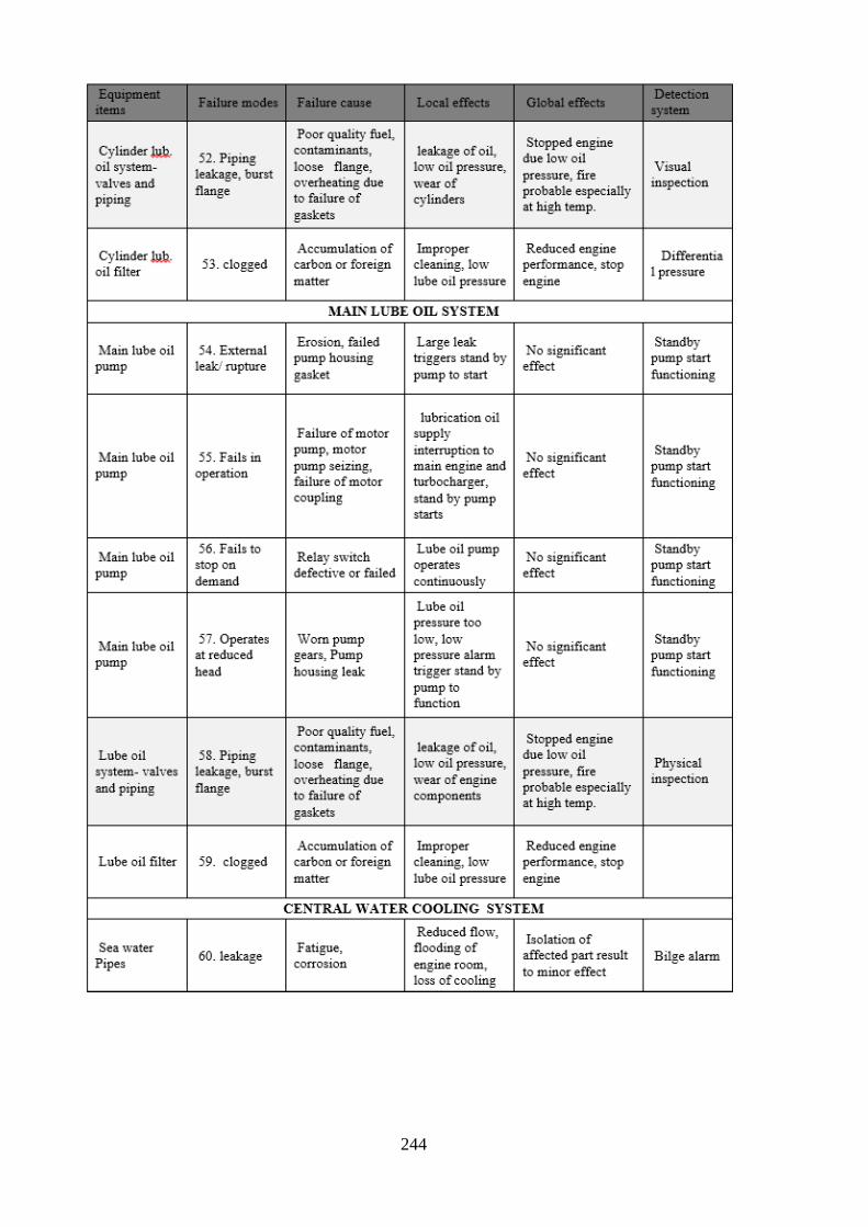
244

245

246

A.2 Expert assigned failure mode rating for the marine diesel engine

247

248

A.3 Decision matrix for failure modes of the marine diesel engine

249

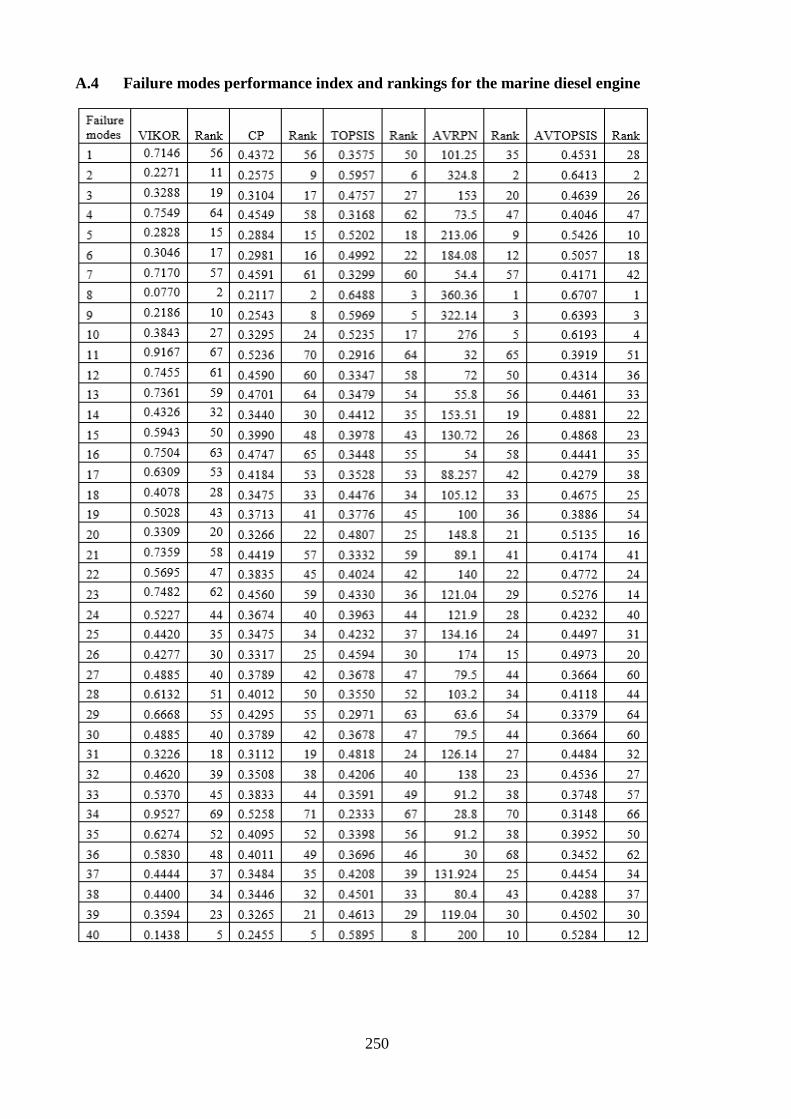
250

A.4 Failure modes performance index and rankings for the marine diesel engine

251

252

Appendix B: Maintenance Strategy Selection

B.1 Delphi Survey Questionnaire

The Delphi survey questionnaires sent to 10 experts in the first and second rounds are

presented in B.1.1 and B1.2 respectively.

B.1.1 Delphi Survey Round 1 Questionnaire

Dear Sir/Madam,

I am a PhD Research Student at Newcastle University conducting research entitled,

DEVELOPMENT OF A METHODOLOGY FOR SELECTING OPTIMAL

MAINTENANCE STRATEGIES FOR MARINE SYSTEMS

The Research Aim is to develop a holistic methodology to enable plant managers to select an

optimal maintenance strategy for each piece of equipment in the marine machinery system

from a set of possible alternatives. In our approach we are embedding Multi-Criteria Decision

Making tool (Analytic Hierarchy process) within the Reliability Centered Maintenance

framework, for selecting maintenance strategy for failure mechanisms of a marine machinery

system.

As part of the effort to achieve the research objectives I would like you to kindly take a few

minutes to respond to this questionnaire. All information provided will be used for academic

statistical analysis only and the data source will be kept anonymous. Therefore please feel at

ease in filling out the answers. Please note that this is the first round of questionnaire; the

second round of questionnaire (summary of result of first round questionnaire) will be

forwarded to you in four weeks’ time.

Table B1 on page 2 is a list of proposed criteria for selecting the maintenance strategy in

addressing potential failure mechanisms of a marine diesel engine and diesel generator. Please

rate each of the criteria with respect to its value in determining the appropriate maintenance

strategy for each component of the system, where 1 indicates not necessary, 2 indicates

useful but not essential and 3 indicates essential.

253

Table B1 Round 1 Delphi survey questionnaire

254

2. If you have any suggestion of any criteria for selecting maintenance strategy not listed in

the above 22 criteria, please list below:

………………………………………………………………………………………….

………………………………………………………………………………………….

………………………………………………………………………………………….

………………………………………………………………………………………….

………………………………………………………………………………………….

………………………………………………………………………………………….

B1.2 Delphi Survey Round 2 Questionnaire

Dear Sir/Madam,

I wish to thank you for your participation and prompt response in the first round of the Delphi

survey. As stated in the first survey, the Delphi method is an iterated technique for processing

opinions of experts till a reasonable consensus is reach on the subject under investigation.

Please re-evaluate the second round questionnaire in Table 1 (Note: it is the same

questionnaire in the first round I sent to you four weeks ago) with the knowledge of the

summary of results of the ten-man experts’ responses you inclusive from the first round

presented in Table 2.

The summary of results presented in Table 2 shows the average or mean and the standard

deviation of scores returned by ten experts for each of the proposed maintenance selection

strategy criteria for marine diesel engine using a three point scale in which 1 indicates not

necessary, 2 indicates useful but not essential and 3 indicates essential. From the result

using the Delphi elimination rule, criteria with mean value below 2.7 is dropped. Based on

this rule the following maintenance selection criteria will be eliminated:

1. Planning flexibility

2. Compatibility

3. Acceptance by labour

4. Availability

5. Manufacturer’s recommendation

6. Image damage

7. Assurance.

255

Table B2 Round 2 Delphi survey questionnaire

256

2. If you have any comments, please state below:

………………………………………………………………………………………….

………………………………………………………………………………………….

………………………………………………………………………………………….

………………………………………………………………………………………….

B.2: Survey Questionnaire for the development of the AHP model for maintenance

strategy selection for marine machinery systems

Dear Sir/Madam,

The purpose of this questionnaire is to perform a pair comparison judgement of three different

maintenance strategies; corrective maintenance, preventive maintenance and condition based

maintenance with respect to evaluation criteria in order to choose the most appropriate

strategy for maintaining sea water pump of a central cooling system of a marine diesel engine.

In order words, your opinions is being sort in deciding on the most appropriate maintenance

strategy for maintaining sea water pump of a central cooling system of a marine diesel engine.

Kindly take some of your precious time to respond to question 1, 2 and 3 and freely express

your opinion by marking X in the appropriate column as your response will be treated

anonymously and only be used for statistical analysis.

We will appreciate if you respond as soon as possible.

Thanks for your anticipated cooperation.

Question 1. Perform pairwise comparison of main criteria with respect to the main goal;

maintenance strategy selection.

For Table B3 carry out a pair wise comparison of main criteria for selecting maintenance

strategy for sea water pump of a central cooling system of a marine diesel engine. If the main

criterion on the left column of the table is more important to the one on the right, mark X to

the left of ‘Equal’ otherwise mark to the right and if they are of equal importance mark X on

‘Equal’.

257

Question 2. Perform pairwise comparison of sub-criteria with respect to 4 main criteria and

bearing in mind the main objective.

Do a pairwise comparison of sub-criteria in Tables 2 to 5 with respect to main criteria. If the

sub-criterion on the left column of the table is more important to the one on the right, mark X

to the left of ‘Equal’ otherwise mark to the right and if they are of equal importance mark X

on ‘Equal’.

Question 3. Perform a Pairwise comparison of maintenance strategy with respect to 16

criteria and having in mind the main goal.

For each criterion in Tables 6 to 20 compare the maintenance strategy on the left column to

the one on the right column. If a maintenance strategy on the left column is more important to

the one on the right, mark X to the left of ‘Equal’ otherwise mark to the right and if they are

of equal importance in maintaining sea water pump of a central cooling system of marine

diesel engine with respect to a criterion mark X on ‘Equal’.

Table B3: Importance of one main criterion over another with respect to selection of

maintenance strategy

258

Table B4: Importance of one sub-criterion over another with respect to main criterion 1 (Cost)

Table B5: Importance of one sub-criterion over another with respect to main criterion 2

(Safety)

Table B6: Importance of one sub-criterion over another with respect to main criterion 3

(Added value)

259

Table B7: Importance of one sub-criterion over another with respect to main criterion 4

(Applicability)

Table B8: Importance of one maintenance strategy over another with respect to criterion

Spare parts inventories costs

260

Table B9: Importance of one maintenance strategy over another with respect to criterion

Maintenance cost

Table B10: Importance of one maintenance strategy over another with respect to criterion

Crew training cost

261

Table B11: Importance of one maintenance strategy over another with respect to criterion

Equipment damage cost

Table B12: Importance of one maintenance strategy over another with respect to criterion

Personnel safety

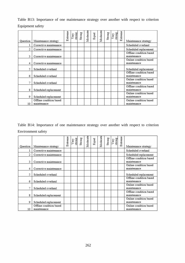
262

Table B13: Importance of one maintenance strategy over another with respect to criterion

Equipment safety

Table B14: Importance of one maintenance strategy over another with respect to criterion

Environment safety

263

Table B15: Importance of one maintenance strategy over another with respect to criterion

Minimisation of operation loss

Table B16: Importance of one maintenance strategy over another with respect to criterion

Equipment reliability

264

Table B17: Importance of one maintenance strategy over another with respect to criterion

System failure characteristics

Table B18: Importance of one maintenance strategy over another with respect to criterion

Available monetary resource

265

Table B19: Importance of one maintenance strategy over another with respect to criterion

Equipment risk level

B.3 Comparison judgement from three experts

B3.1 Comparison judgement for AHP models obtained from expert 1

Table B20: Sub-criteria comparison matrix with respect to safety

Table B21: Sub-criteria comparison matrix with respect to added value

266

Table B22: Sub-criteria comparison matrix with respect to applicability

Table B23: maintenance alternatives comparison matrix with respect to sub-criterion

maintenance cost

Table B24: maintenance alternatives comparison matrix with respect to sub-criterion Crew

training cost

Table B25: maintenance alternatives comparison matrix with respect to sub-criterion

equipment damage cost

267

Table B26: maintenance alternatives comparison matrix with respect to sub-criterion

personnel safety

Table B27: maintenance alternatives comparison matrix with respect to sub-criterion

equipment safety

Table B28: maintenance alternatives comparison matrix with respect to sub-criterion

environment safety

Table B29: maintenance alternatives comparison matrix with respect to sub-criterion

minimisation of operation loss

268

Table B30: maintenance alternatives comparison matrix with respect to sub-criterion

equipment reliability

Table B31: maintenance alternatives comparison matrix with respect to sub-criterion

equipment failure characteristics

Table B32: maintenance alternatives comparison matrix with respect to sub-criterion available

monetary resources

Table B33: maintenance alternatives comparison matrix with respect to sub-criterion

equipment risk level

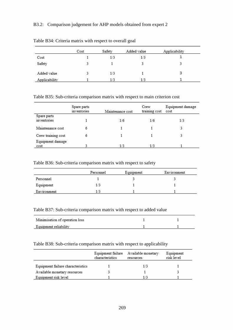
269

B3.2: Comparison judgement for AHP models obtained from expert 2

Table B34: Criteria matrix with respect to overall goal

Table B35: Sub-criteria comparison matrix with respect to main criterion cost

Table B36: Sub-criteria comparison matrix with respect to safety

Table B37: Sub-criteria comparison matrix with respect to added value

Table B38: Sub-criteria comparison matrix with respect to applicability

270

Table B39: maintenance alternatives comparison matrix with respect to sub-criterion spare

parts inventories cost

Table B40: maintenance alternatives comparison matrix with respect to sub-criterion

maintenance cost

Table B41: maintenance alternatives comparison matrix with respect to sub-criterion Crew

training cost

Table B42: maintenance alternatives comparison matrix with respect to sub-criterion

equipment damage cost

271

Table B43: maintenance alternatives comparison matrix with respect to sub-criterion

personnel safety

Table B44: maintenance alternatives comparison matrix with respect to sub-criterion

equipment safety

Table B45: maintenance alternatives comparison matrix with respect to sub-criterion

environment safety

Table B46: maintenance alternatives comparison matrix with respect to sub-criterion

minimisation of operation loss

272

Table B47: maintenance alternatives comparison matrix with respect to sub-criterion

equipment reliability

Table B48: maintenance alternatives comparison matrix with respect to sub-criterion

equipment failure characteristics

Table B49: maintenance alternatives comparison matrix with respect to sub-criterion available

monetary resources

Table B50: maintenance alternatives comparison matrix with respect to sub-criterion

equipment risk level

273

B3.3: Comparison judgement for AHP models obtained from expert 3

Table B51: Criteria matrix with respect to overall goal

Table B52: Sub-criteria comparison matrix with respect to main criterion cost

Table B53: Sub-criteria comparison matrix with respect to safety

Table B54: Sub-criteria comparison matrix with respect to added value

274

Table B55: Sub-criteria comparison matrix with respect to applicability

Table B56: maintenance alternatives comparison matrix with respect to sub-criterion spare

parts inventories cost

Table B57: maintenance alternatives comparison matrix with respect to sub-criterion

maintenance cost

Table B58: maintenance alternatives comparison matrix with respect to sub-criterion Crew

training cost

275

Table B59: maintenance alternatives comparison matrix with respect to sub-criterion

equipment damage cost

Table B60: maintenance alternatives comparison matrix with respect to sub-criterion

personnel safety

Table B61: maintenance alternatives comparison matrix with respect to sub-criterion

equipment safety

Table B62: maintenance alternatives comparison matrix with respect to sub-criterion

environment safety

276

Table B63: maintenance alternatives comparison matrix with respect to sub-criterion

minimisation of operation loss

Table B64: maintenance alternatives comparison matrix with respect to sub-criterion

equipment reliability

Table B65: maintenance alternatives comparison matrix with respect to sub-criterion

equipment failure characteristics

Table B66: maintenance alternatives comparison matrix with respect to sub-criterion available

monetary resources

277

Table B67: maintenance alternatives comparison matrix with respect to sub-criterion

equipment risk level

B.4: Questionnaire produce to obtained information for PROMETHEE and TOPSIS

Dear Sir,

The purpose of this questionnaire is to determine the most appropriate maintenance strategy

from among five maintenance alternatives for sea water pump of a central cooling system of a

marine diesel engine. The five maintenance strategies are: Corrective maintenance (CM),

Scheduled overhaul (SOH), Scheduled replacement (SRP), Offline-Condition based

maintenance (OFCBM) and Online-Condition based maintenance (ONCBM).

Please rank the five maintenance strategies with respect to the 4 decision criteria using a 5

point Likert scale i.e.1 to 5. Ranking score 1 represent very bad and 5 represent very good.

Note lower cost is preferred to higher cost and higher benefit is preferred to lower benefit.

For example considering criteria cost; if I rate Corrective maintenance (CM), Scheduled

overhaul (SOH), Scheduled replacement (SRP), Offline-Condition based maintenance

(OFCBM) and Online-Condition based maintenance (ONCBM) to be 5, 4, 3, 2 and 1

respectively; it means applying corrective maintenance will result to lowest spare parts

inventories cost while applying Online-Condition based maintenance will result to highest

spare parts inventories cost. Also considering criteria AV2; Corrective maintenance (CM),

Scheduled overhaul (SOH), Scheduled replacement (SRP), Offline-Condition based

maintenance (OFCBM) and Online-Condition based maintenance (ONCBM) to be 1, 2, 3, 4

and 5 respectively; it means condition based maintenance will result to best equipment

reliability and corrective maintenance least equipment reliability while others are in between.

278

Table B68: PROMOTHEE and TOPSIS questionnaire

279

Appendix C: Scheduled Replacement Interval Determination

C.1: Matlab Program for calculating Reliability function, Cost function and

Downtime function

b=3.432;a=31699;ca=8000;cb=2000;Ta=3;Tb=15; % input data

f=@(x)(x.*((b./a).*((x./a).^(b-1)).*exp((-(x./a).^b)))); % probability density function

calculation

j=5000:1000:34000; % replacement alternative intervals

tp=zeros(1,length(j));q=zeros(1,length(j));Rtp=zeros(1,length(j));Ctp=zeros(1,length(j));Dtp=

zeros(1,length(j));

t=zeros(1,length(j));

for i=1:length(j);

tp=j(i);

t(i)=tp;

q(i)=quadgk(f,0,t(i));

Rtp(i)=exp(-(t(i)/a).^b); % Reliability per unit time calculation

Ctp(i)=(ca.*(1-Rtp(i))+cb.*Rtp(i))/(q(i)+Tb.*(1-Rtp(i))+(Ta+t(i)).*Rtp(i)); % cost per unit

time calculation

Dtp(i)=(Tb.*(1-Rtp(i))+Ta.*Rtp(i))/(q(i)+(Tb.*(1-Rtp(i)))+(Ta+t(i)).*Rtp(i)); % Downtime

per unit time calculation

end

figure;plot(t,Ctp,'bo','linewidth',1.0)

title('cost vs time');xlabel('time(tp(s))');ylabel('Ctp')

figure;plot(t,Dtp,'bo','linewidth',1.0)

title('downtime vs time')

figure;plot(t,Rtp,'bo','linewidth',1.0)

title('reliabilty vs time')

280

C.2 Sensitivity analysis of parameters of decision criteria

Table C1: TOPSIS performance index of sensitivity analysis β

281

Table C2 Ranking of sensitivity analysis of β

282

Table C3: TOPSIS Performance index of sensitivity analysis of ϕ

283

Table C4: Ranking of sensitivity analysis of ϕ

284

Table C5: TOPSIS performance index of sensitivity analysis of cost ratio

285

Table C6: Ranking of sensitivity analysis of cost ratio

286

Table C7: TOPSIS performance index of sensitivity analysis of ratio of Tb to Ta

287

Table C8: Ranking of sensitivity analysis of ratio of Tb to Ta

288

Appendix D: Inspection Interval Determination

D.1 Matlab Program for determining D(T), C(T) and R(T) under various delay time

failure distribution

% % % % % WEILBUL DISTRIBUTION ROUTINE

d=0.2083;k=0.001277;db=168;a=5;b=10;CB=52000;CIR=10500;CI=210;ld=0.1;RBR=10;RII

=1;

q=zeros(1,length(j));DT=zeros(1,length(j));CT=zeros(1,length(j));q1=zeros(1,length(j));q2=z

eros(1,length(j))

j=1:2:50;

ms=3; %markere size

for i=1:length(j);

T=j(i);

t(i)=T(:,1);

f=@(h)((T-h).*((a./b).*((h./b).^(a-1)).*exp((-(h./b).^a))));

q(i)=1./T*integral(f,0,T);

CTw(i)=(k*T*(CB.*q(i)+CIR.*(1-q(i)))+CI)./(T+d);

RTw(i)=(k*T*(RBR.*q(i)+RII.*(1-q(i))))./(T+d);

DTw(i)=((d+k.*T.*q(i)).*db)./(T+d);

end

figure;plot(t,CTw,'-bo','linewidth',1.0,'MarkerSize',ms)

title('cost vs time');xlabel('time(T(s))');ylabel('CTw');

figure;plot(t,RTw,'bo','linewidth',1.0,'MarkerSize',ms)

title('Reputation vs time');xlabel('time(T(s))');ylabel('RTw')

figure;plot(t,DTw,'-bo','linewidth',1.0,'MarkerSize',ms)

title('downtime vs time');xlabel('time(T(s))');ylabel('DTw')

% % % % % EXPONENTIAL DISTRIBUTION ROUTINE

for i=1:length(j);

T=j(i);

t(i)=T(:,1);

f1=@(h)((T-h).*(ld*exp(-ld*h)));

q1(i)=1./T*integral(f1,0,T);

289

CTe(i)=(k*T*(CB.*q1(i)+CIR.*(1-q1(i)))+CI)./(T+d);

RTe(i)=(k*T*(RBR.*q1(i)+RII.*(1-q1(i))))./(T+d);

DTe(i)=((d+k*T.*q1(i)).*db)./(T+d);

end

figure;plot(t,CTe,'-bo','linewidth',1.0,'MarkerSize',ms)

title('cost vs time');xlabel('time(T(s))');ylabel('CTe')

figure;plot(t,RTe,'-bo','linewidth',1.0,'MarkerSize',ms)

title('Reputation vs time');xlabel('time(T(s))');ylabel('RTe')

figure;plot(t,DTe,'-bo','linewidth',1.0,'MarkerSize',ms)

title('downtime vs time');xlabel('time(T(s))');ylabel('DTe')

% % % % % NORMAL DISTRIBUTION ROUTINE

for i=1:length(j);

T=j(i);

t(i)=T(:,1);

f2=@(h)((T-h)./T).*((2/((2*pi)^(0.5)).*exp(-(h.^2)/2)));

q2(i)=integral(f2,0,T);

CTn(i)=(k*T.*(CB.*q2(i)+CIR.*(1-q2(i)))+CI)./(T+d);

RTn(i)=(k*T*(RBR.*q2(i)+RII.*(1-q2(i))))./(T+d);

DTn(i)=((d+k*T.*q2(i))*db)/(T+d);

end

figure;plot(t,CTn,'-bo','linewidth',1.0,'MarkerSize',ms)

title('cost vs time');xlabel('time(T(s))');ylabel('CTn')

figure;plot(t,RTn,'-bo','linewidth',1.0,'MarkerSize',ms)

title('Reputation vs time');xlabel('time(T(s))');ylabel('RTn')

figure;plot(t,DTn,'-bo','linewidth',1.0,'MarkerSize',ms)

title('downtime vs time');xlabel('time(T(s))');ylabel('DTn')

figure;plot(t,DTw,'-or',t,DTe,'-*b',t,DTn,'-dk','linewidth',1.0,'MarkerSize',ms)

title('downtime vs

time');xlabel('time(T(s))');ylabel('DTw,DTe,DTn,(hr)');legend('Weilbul','Exponential','Normal'

)

figure;plot(t,CTw,'-or',t,CTe,'-*b',t,CTn,'-dk','linewidth',1.0,'MarkerSize',ms)

title('costvs

time');xlabel('time(T(s))');ylabel('CTw,CTe,CTn,(hr)');legend('Weilbul','Exponential','Normal'

)

290

figure;plot(t,RTw,'-or',t,RTe,'-*b',t,RTn,'-dk','linewidth',1.0,'MarkerSize',ms)

title('Reputation vs

time');xlabel('time(T(s))');ylabel('RTw,RTe,RTn,(hr)');legend('Weilbul','Exponential','Normal'

)

D.2 Computer programme for the ELECTRE method

tic

% enter criteria vector

C1=[1350; 1680; 1560; 1470]; %; 256];

C2=[1850; 1650; 1950; 1850]; %; 610];

C3=[7.5; 8.5; 6.5; 9.5];%; 60];

C4=[2.58; 3.75; 4.86; 3.16];%; 86];

C5=[93.5; 95.3; 88.6; 98.4];% 89];

C6=[0.045; 0.068; 0.095; 0.072];%; 0.01];

% C7=[2.75; 2.63; 2.5; 4; 2.59];

% Enter Criteria weights

w=[0.2336 0.1652 0.3355 0.1021 0.0424 0.1212];

Wcheck=sum(w(:)); % Wcheck=1

%length of a CRITERIA matrix is the same as the number of alternatives

% build the decision matrix D

% CONCATENATE CRITERIA TO FORM DECISION MATRIX D

D=[C1 C2 C3 C4 C5 C6];% C7] % Size of D is no. of alternative by no. of criteria

L=size(D);

LA=size(D,1); %NUMBER OF ALTERNATIVE

LC=size(D,2); %NUMBER OF CRITERIA

% normalize the Decision Matrix D

j=1:LC;

SumD=(sum((D(:,j).^2))).^0.5;

% SumD=sum(D(:,j)); % Alternative Normalizing technique

291

r=zeros(); V=zeros(); %pre-allocation

for i=1:LA

for j=1:LC;

r(i,j)=D(i,j)/SumD(j); % Normalized MATRIX

V(i,j)=r(i,j).*w(j); % Weight Normalized MATRIX

end

end

%Concordance calculation

wc=w;

for i=1:LA

for i1=LA:-1:1

E1=V(i,:);

E2=V(i1,:);

E12=[];

for j=1:LC;

a=E1(1,j);

b=E2(1,j);

if a>=b;

E12_1=j;

else

E12_1=0;

end

E12=[E12 E12_1];

for k=1:length(E12)

if E12(k)==0;

wc(k)=0;

else

wc(k)=w(k);

end

end

EC=sum(wc(:));

% RETURN ZERO FOR ALL DIAGONAL MATRIX ELEMENT,i.e COMPARING

SAME

292

% ALTERNATIVES

if i==i1

ECM(i,i1)=0;

else

ECM(i,i1)=EC;

end

end

end

end

%DISCONCORDANCE calculation

% wc=w;

for i=1:LA

for i1=LA:-1:1

E1=V(i,:);

E2=V(i1,:);

E12=[];

for j=1:LC;

a=E1(1,j);

b=E2(1,j);

cc=b-a;

c(1,j)=cc;

cmax=max(c(:));

abscmax=max(abs(c(:)));

dd=cmax./abscmax;

end

d(i,i1)=dd;

% RETURN ZERO FOR ALL DIAGONAL MATRIX ELEMENT, i.e. COMPARING

SAME

% ALTERNATIVES

if i==i1

d(i,i1)=0;

else

293

end

end

end

% COMPUTATION OF NET SUPERIOR AND INFERIOR VALUES

ca=zeros(); da=zeros();

for i=1:length(ECM)

ca(i)=sum(ECM(i,:))-sum(ECM(:,i)); %

da(i)=sum(d(i,:))-sum(d(:,i)); %

end

toc

D.3 MATLAB computer program for MAUT analysis

tic

% enter criteria vector

C1=[210; 212; 212; 206.5; 206.5; 187.5; 210; 593; 212.5]; %; 256];

C2=[330; 632.5; 655; 1575; 360; 1825; 1930; 4405; 1655]; %; 610];

C3=[54.5; 46; 87.5; 38; 111.5; 80; 21; 14.05; 120];%; 60];

C4=[0.00111; 0.00117; 0.000515; 0.00026; 0.00089; 0.00071; 0.00002055; 0.00135;

0.00113];%; 86];

C5=[150; 355; 305; 483; 190; 532.5; 771; 1250; 448.5];% 89];

C6=[0.673; 0.7045; 0.864; 1.175; 0.8665; 6.97; 7.99; 79.6; 1.73];%; 0.01];

% C7=[2.75; 2.63; 2.5; 4; 2.59];

% Enter Criteria weights

w=[0.291 0.079 0.206 0.188 0.098 0.139];

Wcheck=sum(w(:)); % Wcheck=1

%length of a CRITERIA matrix is the same as the number of alternatives

% build the decision matrix D

% CONCATENATE CRITERIA TO FORM DECISION MATRIX D

D=[C1 C2 C3 C4 C5 C6];% C7] % Size of D is no. of alternative by no. of criteria

294

L=size(D);

LA=size(D,1); %NUMBER OF ALTERNATIVE

LC=size(D,2); %NUMBER OF CRITERIA

%Input alternative inspection

Tmin=50;

Tmax= 300;

% Tinterval=0.55;

% T=Tmin:Tintval:Tmax;

T=linspace(Tmin,Tmax,length(C1));

R=1; % Factor that determines the decision maker RISK Perception

% Standardize the D matrix

for j=1:LC%

for i=1:LA

U(i,j)=((D(i,j)-min(D(:,j)))/range(D(:,j)))^R;

u(i,j)=U(i,j)*w(j); %weight factor multiplied standardized matrix U.

A(i)=sum(u(i,:)); %Alternatives evaluation

end

end

figure; plot(T,A,'-*b') ;title('plot of ... vs ...'),xlabel('T ,,,,'),ylabel('A''''')'

legend('A')

295

D.4: Sensitivity Analysis of decision criteria weight on MAUT and ELECTRE methods

Table D1: sensitivity analysis of R on MAUT method

296

Table: D2 Sensitivity analysis of decision weights on MAUT method

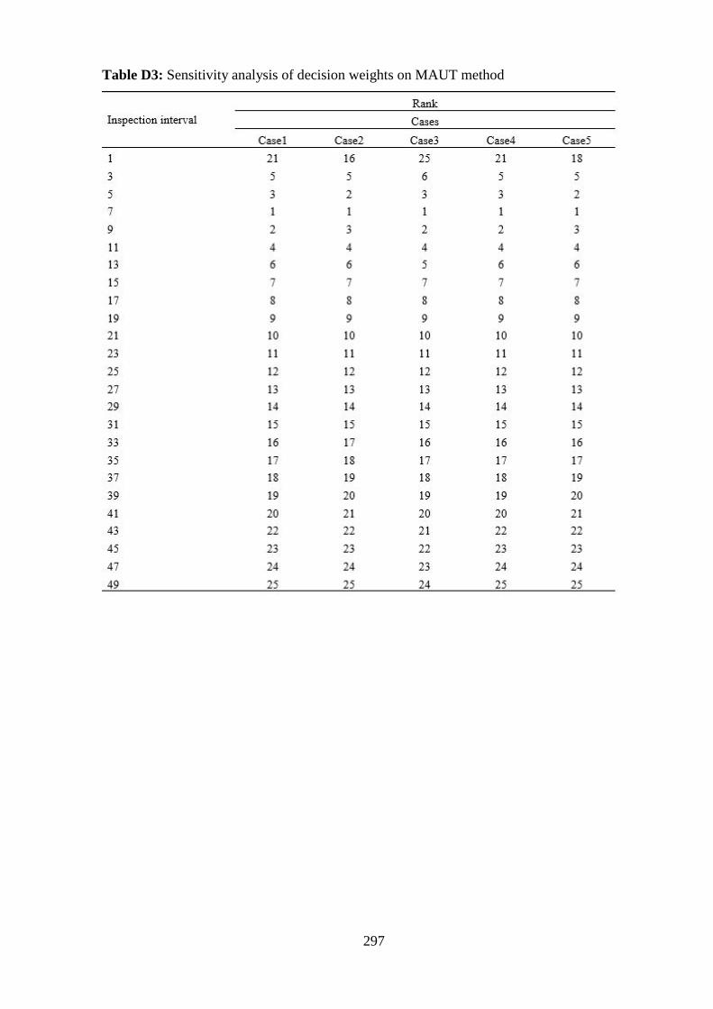
297

Table D3: Sensitivity analysis of decision weights on MAUT method

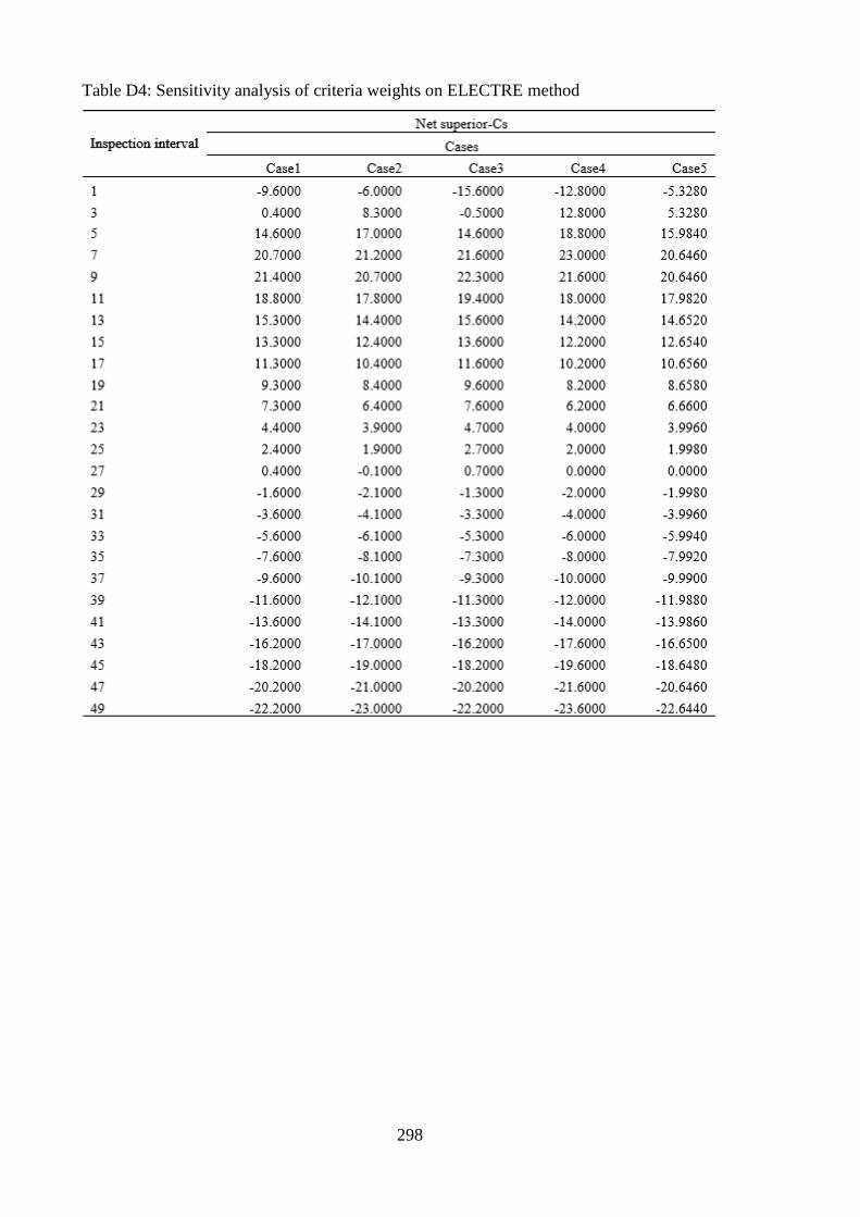
298

Table D4: Sensitivity analysis of criteria weights on ELECTRE method

299

Table D5: Sensitivity analysis of criteria weights on ELECTRE method

300

Table D6: Sensitivity analysis of criteria weights on ELECTRE method

301

Table D7: Sensitivity analysis of criteria weights on ELECTRE method