Multi-class image segmentation using Conditional Random Fields

Multi-class image segmentation using Conditional Random Fieldsand Global Classification

Nils Plath [email protected] Toussaint [email protected]

TU Berlin, Machine Learning Group, Franklinstrasse 28/29, D-10587 Berlin, Germany

Shinichi Nakajima [email protected]

Nikon Corporation, Optical Research Laboratory, 1-6-3 Nishi-Ohi, Shinagawa-ku, Tokyo 140-8601, Japan

Abstract

A key aspect of semantic image segmenta-tion is to integrate local and global featuresfor the prediction of local segment labels.We present an approach to multi-class seg-mentation which combines two methods forthis integration: a Conditional Random Field(CRF) which couples to local image featuresand an image classification method whichconsiders global features. The CRF followsthe approach of Reynolds & Murphy (2007)and is based on an unsupervised multi scalepre-segmentation of the image into patches,where patch labels correspond to the ran-dom variables of the CRF. The output of theclassifier is used to constraint this CRF. Wedemonstrate and compare the approach on astandard semantic segmentation data set.

1. Introduction

Visual scene understanding, e.g., in a robotics con-text, means to identify and locate separate objects ina scene. Such a segmentation is a crucial precursor forany object-related behavior, like reaching for an ob-ject, moving towards an object or telling a user wherean object is located. Even without depth informa-tion (disparity, motion) humans are extremely goodin segmenting still images whereas this is still a greatchallenge for Machine Learning (ML) methods (Ever-ingham et al., 2008).

An interesting issue in this context is that most state-of-the-art ML methods for image classification – that

Appearing in Proceedings of the 26 th International Confer-ence on Machine Learning, Montreal, Canada, 2009. Copy-right 2009 by the author(s)/owner(s).

is, the task of predicting whether an object from a cer-tain class is contained in the image – rely completelyon global image features (Zhang et al., 2007), since ata local level the discriminating appearance of imagepatches will deteriorate (e.g., wheels can be parts ofvarious kinds of vehicles.) Hence, typical image classi-fication methods do not attempt to locate the objector use information from a special focal area. Theyonly predict the presence of an object, in some sensewithout knowing where it is. This fact suggests twoimplications. First, the object context seems equallyrelevant for the prediction as the object area itself.Second, although image segmentation is the problemof assigning a local object label to every local pixel, wemay expect that a purely local mapping will not per-form well because the work on classification demon-strates the importance of the context.

In this paper we propose a method for multi-class im-age segmentation which comprises two aspects for cou-pling local and global evidences. First, we formulate aConditional Random Field (Lafferty et al., 2001) thatcouples local segmentation labels in a scale hierarchy.This idea follows largely previous work by (Reynolds& Murphy, 2007), which we extend to the multi-classcase and the use of SVMs to provide the local patchevidences. Second, we use global image classificationinformation to decide prior to the segmentation pro-cess which segment labels are considered possible in agiven new image. Experiments show that without thisuse of global classification, the segmentation performspoorly. However, with a hypothetical optimal classi-fication the segmentation outperforms the best state-of-the-art segmentation algorithms, while it is amongthe top third using our own image classifier.

Previous work on segmentation includes for example(Awasthi et al., 2007). Here, the authors also con-struct a tree structured CRF from image patches. In

Multi-class image segmentation using Conditional Random Fields and Global Classification

contrast to our method, though, they split the im-age into patches laying on a regular grid and connect-ing them using a quad-tree structure. Also, they donot have a image classification step before segmentingan image. Another approach (Csurka & Perronnin,2008) transforms low-level patch features into high-level features based on Fisher kernels and defines ascore system for patches to determine whether a patchis part of fore- or background. Their framework alsoincludes an image classification step, however, no CRFare used (though it could be extended to use CRF).Finally, in (Reynolds & Murphy, 2007) segmentationis facilitated by constructing a tree-structured con-ditional random field on image regions on multiplescales. Their method is able to segment objects anddivide image into fore- and background. In its orig-inal form it is only applicable to two-class scenarios,foreground and background. We extend this to themulti-class case and introduce an image classificationstep to improve segmentation results.

Our segmentation algorithm follows a number of stepswhich we briefly summarize here:

1. We first use an unsupervised segmentation to frag-ment the whole image in a number of patches onmultiple scale levels.

2. For each patch on each level we compute color,texture and SIFT features.

3. From all patch features we also compute a globalimage feature vector.

4. We use trained SVMs to predict a class member-ship for each patch and for the whole image.

5. Depending on the image structure and the globalclassification we build a CRF model – a depen-dency tree between patch labels – and use theSVMs outputs as local evidences in this .

6. Thresholding the posterior labels for the finestpatches produces the final segmentation.

The next section describes the unsupervised imagesegmentation and the feature computation. Section3 will explain the CRF model, how we train it andhow we use the global classification. Section 4 demon-strates the approach on the challenging PASCAL VOC2008 image segmentation data set (Everingham et al.,2008).

2. Pre-segmentation and Features

2.1. Unsupervised pre-segmentation intoimage patches

The aim of unsupervised image segmentation is to seg-ment the image into patches of high textural and colorhomogeneity. This kind of segmentation is a priori in-dependent from any given labels or object classes, butdue to the textural and color homogeneity, the result-ing patches are likely to belong to only one object andnot overlap with different objects. Felzenszwalb andHuttenlocher (2004) proposes an algorithm based on agraph cut minimization formulation: Every pixel of animage is considered a node of a graph. Starting withan initially unconnected graph, a greedy algorithm de-cides on whether to connect nodes/pixels (and therebysubgraphs/patches) depending on their similarity anddepending on evidence that there actually is a visualboundary between those patches.

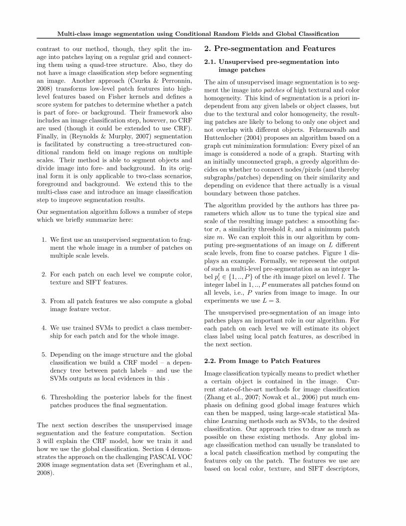
The algorithm provided by the authors has three pa-rameters which allow us to tune the typical size andscale of the resulting image patches: a smoothing fac-tor σ, a similarity threshold k, and a minimum patchsize m. We can exploit this in our algorithm by com-puting pre-segmentations of an image on L differentscale levels, from fine to coarse patches. Figure 1 dis-plays an example. Formally, we represent the outputof such a multi-level pre-segmentation as an integer la-bel pli ∈ {1, .., P} of the ith image pixel on level l. Theinteger label in 1, .., P enumerates all patches found onall levels, i.e., P varies from image to image. In ourexperiments we use L = 3.

The unsupervised pre-segmentation of an image intopatches plays an important role in our algorithm. Foreach patch on each level we will estimate its objectclass label using local patch features, as described inthe next section.

2.2. From Image to Patch Features

Image classification typically means to predict whethera certain object is contained in the image. Cur-rent state-of-the-art methods for image classification(Zhang et al., 2007; Nowak et al., 2006) put much em-phasis on defining good global image features whichcan then be mapped, using large-scale statistical Ma-chine Learning methods such as SVMs, to the desiredclassification. Our approach tries to draw as much aspossible on these existing methods. Any global im-age classification method can usually be translated toa local patch classification method by computing thefeatures only on the patch. The features we use arebased on local color, texture, and SIFT descriptors,


(a) (b) (c) (d)

Figure 1. Images are segmented with a greedy algorithm at multiple scales. Each patch q at level l is connected to the onenode p in the next coarser level l+ 1 which has the largest overlap with itself. In this example three tree are constructedfor this image.

which we explain in the following.

The color features are computed from the HSV colorspace model of the input image. As in (Reynolds &Murphy, 2007) we compute an HSV histogram over animage patch where hue and saturation are binned to-gether into a 10×10-bin histogram and value is binnedseparately into a 10-bin histogram. For each patchp ∈ {1, .., P} this gives a feature vector f color

p ∈ R110.

The texture features are computed using Gabor filters.Also as in (Reynolds & Murphy, 2007) we applied thesefilters to the images with d = 6 directions and at s =4 scales. The resulting energies are binned on a perpatch-basis in a 10-bin histogram for each directionand scale, which gives a feature vector f texture

p ∈ R240.

Finally, for standard image classification bag-of-wordsfeatures based on SIFT descriptors have been foundcritical for high performances. We first compute astandard SIFT discriptor at regular grid points overthe whole image. We choose a grid width of 6 pixelsso that the local SIFT circular regions, with a radius of16 pixels, overlap. We assume that during training wehave created a visual codebook of SIFT descriptors,i.e., we have clustered the SIFT data to yield 1000visual prototypes using regular K-Means. Hence, ateach grid point we can associate the computed SIFTdiscriptor with an integer i ∈ {1, .., 1000} indicatingthe prototype it belongs to. To construct the patchfeature, we consider all the grind points in a givenpatch and compute the prototype histogram. Since wechoose a small enough grid size and sufficiently highminimum patch size k we never observed that a patchwithout any grid points in practice. For each patch pthis gives a feature vector fSIFT

p ∈ R1000.

The full patch feature fp = (f colorp , f texture

p , fSIFTp ) is

the concatenation of the described features.

As mentioned in the introduction, the local classifi-cation inherent in image segmentation can profit fromthe global classification of the whole image because the

latter is a compact representation of the context. Wewill make use of global image classification and hencealso need to define global image features. As before wedefine a regular grid over the images, here with a 10pixel width, and compute SIFT descriptors over mul-tiple scales, i.e. the radii are changed on each layer (4,6, 8, and 16 pixels). Then visual prototypes are con-structed with K-Means clustering. For computationalreasons we randomly selected 10 images from each ob-ject class and computed 1200 cluster centers followedby a quantization of the image features. Additionallywe computed a 2-level spatial pyramid representationof the images, which has been shown to perform well in(Lazebnik et al., 2006). The final image-level featurevector is the concatenation of all histograms over allregions in the pyramid and over all scales. The train-ing of the image classifier makes use of a SVM with aχ2 kernel. The details of training are the same as forthe segmentation, as will be explained later.

3. Conditional Random Fields

The patch features allow us to learn a patch classi-fier that would predict the object class membership ofeach patch independently. However, given the spatialrelation between patches – and in particular the re-lation (overlap) between patches on the different scalelevels – the patch labels should not be considered inde-pendent. A standard framework for the prediction ofdependent labels of multiple output variables is struc-tured output regression (Lafferty et al., 2001; Altunet al., 2003; Tsochantaridis et al., 2005). Generally,a discriminative function F (y, x) over all output vari-ables y = (y1, .., yP ) is defined depending on the inputx such that the prediction for all output variables isgiven as f(x) = argminy F (y, x). The factorization ofF (y, x) w.r.t. y typically corresponds to a graphicalmodel for which the argmin can efficiently be com-puted using inference methods.

Let us first focus on only one object class, N = 1;


we will discuss the general multi-class segmentationbelow. In this case we need to segment the imageinto foreground (label 1) and background (label 0).We will predict these labels not on the level of pixelsbut on the level of patches. Hence, in our case theoutput variables y = (y1, .., yP ) are the binary labelsyp ∈ {0, 1} we want to predict for each patch.

We assume a tree as the coupling structure betweenthese variables. Let π(p) denote the set of children(descending nodes) of a patch p in this tree, then thediscriminative function is of the form

F (y, x) =P∏p=1

φ(yp, x)∏

q∈π(p)

ψ(yp, yq) , (1)

where φ(yp, x) represents input dependent evidencesfor each patch, and ψ(yp, yq) represents a pair-wisecoupling between the labels of a parent and childpatch. We first explain how we construct the tree for aspecific image before giving details on these potentials.

The tree (actually forest) is fully defined by specify-ing the parent of each node. A node corresponds toa patch from one of the multiple scale levels. Everypatch connects to the one parent patch in the nextcoarser level which has the largest overlap with itself:if q is a patch of level l, then its parent p in level l+ 1is

p = argmaxp

|Ip ∩ Iq||Iq|

, (2)

where Ip = {i ∈ I : pl+1i = p} is the image region

that corresponds to p. As a result, every patch in thecoarsest level does not have a parent and is a root ofa tree. Figure 1 illustrates such a tree.

The potentials φ(yp, x) represent the local evidence forlabelling the patch p as forground depending on the in-put. We will assume that only the local patch featuresfp are used, φ(yp, x) = φ(yp, fp).

The potentials ψ(yp, yq) describe the pairwise couplingbetween overlapping patched from layers l + 1 and l,respectively. Reynolds and Murphy (2007) made suchedge potentials dependent on the visual similarity be-tween the patches. Although this seems a reasonableheuristic, we found that this local similarity measureis too brittle to yield robust results. We decided touse a set of parameters γl to tune the coupling be-tween pairs of levels separately. This has the advan-tage that the coupling can be increased for layers forwhich the patch-level classifiers exhibit a high amountof certainty. For parent p and child q in layers l + 1and l we define the pairwise potentials as the following

2× 2-matrix

ψ(yp, yq) =(eγl e−γl

e−γl eγl

)(3)

Inference in the tree (or forest) is done using stan-dard exact inference (we use an implementation of theJunction Tree Algorithm).

Concerning the multi-class case we tried some alter-natives. A straight-forward extension to the binarytree is to extend the patchwise labels to be an inte-ger yp ∈ {0, 1, .., N} where N is the number of objectclasses. The local evidences φ(yp, fp) can be repre-sented by N+1 separate models and the pairwise cou-plings ψ(yp, yq) become a (N+1)×(N+1)-matrix withdiagonal entries eγl and constant off-diagonal entriese−γl . This approach seems to work fine if in every im-age we have always all N object classes present. How-ever, in realistic data, some images contain only oneobject class out of N = 20, other images three or more.Generally, the uncertainties in object classes that arenot present in an image cause, particularly for largeN , a significant perturbation of the segmentation ofthe present object class. We decided to aim for a morerobust approach where the segmentation within an ob-ject class should be independent of N and uncertain-ties in other object classes. We settled for having Nseparate binary trees and compute the posterior labeldistribution for each tree. Since we compute patcheson multiple scale levels, we will use the predicted labelsof the smallest scale patches as the predicted segmen-tation. The final label we assign to a patch p is theobject class for which the posterior is maximal if thismaximum is larger than a threshold, and backgroundotherwise. The threshold is determined using cross-validation.

3.1. Training

The conditional random field framework we introducedabove would naturally lead to a structured output re-gression method for training the φ’s and ψ’s. How-ever, we simplified the training problem by decompos-ing the training of local evidences φ(xp, fp) from theinference mechanisms on top of that (Reynolds & Mur-phy, 2007).

We assume we are given a dataset of segmented im-ages, i.e., images for which each pixel i is labeled withan integer Si ∈ {0, .., N} indicating either that thepixel belongs to one of N object classes or to the back-ground (Si = 0). An example is depicted in figure 2.

We can apply the multi-scale pre-segmentation on eachimage of this dataset and compute the patch features


for all patches. When more than 75% of the pixels ofa patch are labelled with the same object class thenwe consider this patch as positive training data for theclassifier for this object class, otherwise it is considerednegative training data (Reynolds & Murphy, 2007).That is, for each patch p = 1, .., P and each object classn = 1, .., N we have a label ypn ∈ {+1,−1} indicatingwhether p has more than 75% overlab with n. We trainN separate SVMs on all patches using these labels ypn.

An appropriate kernel for histogram features is a χ2-kernel, which was shown to be a suitable similaritymeasure histograms features (Hayman et al., 2004;Zhang et al., 2007). The parameter b determines thewidth of the kernel, which is set to the mean of the χ2

distances over all pairs of training samples (Lampert& Blaschko, 2008).

The regularization parameter c was tuned using cross-validation. Since the data is highly biased towardsnegative examples, it is a good idea to duplicate posi-tive training examples so that the number of trainingsamples in both groups is approximately the same. Weused the Shogun SVM implementation (Sonnenburget al., 1999), which balances the data set automati-cally.

Applying a re-normalization using logistic regression(Platt, 1999) allows us to treat the output of the clas-sifiers as probabilities

φ(yp = 1|fp) =1

1 + e−(alsvm(fp)+bl)(4)

where l is the scale level of the patch p and the param-eters al and bl control the slope and the bias.

3.2. Coupling global image classification withlocal segmentation

What we found one of the most important keys to goodimage segmentation is that global image information istaken into account. As discussed in the introduction,the patch classifiers we described in the previous sec-tion rely only on local image information. However,as is evident from the success of image classificationtechniques that neglect completely the location of anobject and use the whole image, the image context isan essential ingredient for good classification. This isalso true for the segmentation task.

Based on the global image feature vector fI we train Nseparate image classifiers (SVMs) to predict whethera certain object class is present in a new image. Onlywhen a class is predicted we build the binary randomtree and consider this class label in the segmentationprocedure described in the previous section.

4. Experiments

In this section we report results on the data set pro-vided by the Pascal VOC2008 challenge (Everinghamet al., 2008). The data set consists of three pre-defined subsets for training, validation, and testing.The groundtruths, as shown in figure 2, are given onlyfor the training and the validation set. However, theorganizers of the challenge offer to evaluate the resultssubmitted to them.

The images, for which the challenge defines 20 objectcategories, are randomly downloaded samples from thefamous Flickr photo portal and the groundtruths wereproduced in meticulous hand-work. On average thetraining and validation set comprise around 40 colorimages per class with varying sizes. No official statis-tics about the test data are published by the organizersof the challenge.

Performance is measured by the average segmentationaccuracy across all object classes and the background.The accuracy a is assessed using the intersection/unionmetric

a =tp

tp + fp + fn(5)

where tp, fp, and fn are true positives, false positives,and false negative, respectively.

Our classification algorithm reached an average preci-sion of 42% on the test data.

The segmentation framework has been set up accord-ing to the parameters in table 1. The initial stageof patch generation involved careful hand-tuning asto satisfy the balance between the number of patchescreated per level and general quality of the patches interms of how they overlap with the actual objects inthe images. Settings for color and texture features re-main the same as in (Reynolds & Murphy, 2007). Theconfiguration for the SIFT components is a trade-offbetween computational efficiency and discriminativefeatures. For the creation of the visual codebook welimited the number of descriptors used and randomlysampled 10, 000 vectors per object class and appliedK-Means clustering.

The entire process chain is shown in figure 4. Thesample images are pre-segmented as described above,then for each patch p in each of the three layers l theconfidence is computed. In figure 4 (b)-(d) the confi-dences for each patch are shown as gray values, whereblack corresponds to a confidence of zero and white toone. The resulting posteriors at the leaf level are illus-trated in figure 4 (e). The last column of this figuredepicts the final segmentation after thresholding the


Table 1. Settings used in experiments. Settings for theclassifiers are not shown, since they are determined auto-matically and may vary depending on the data source.Wetested 3 different segmentation thresholds t, for which allother settings are identical. For tind we computed onethreshold for each object class individually, tglo uses meanof tind, and tmax is set to the maximum of tind.

step parameters values

patchesσl {0.5, 0.75, 1.25}kl {500, 500, 700}ml {50, 200, 1200}

color feat.binsHS 10× 10binsS 10

texture feat.binsGabor 10directionsGabor 6scalesGabor 4

SIFT featuresgrid size 6× 6visual prototypes 1000

treesal {2, 1.5, 1.5}bl {0, 0, 0}γl {2, 1}

BPtind n thresholdstglo mean of tind

tmax max(tind)

posteriors.

Table 2 shows detailed results of our segmentation re-sults and compares them to the competitors of thisyear’s challenge. In average our results settle in themiddle. However, it is important to keep in mind thatour algorithm can only be as good as the prior imageclassification. In a different setting we assumed to havea perfect image classifier. In this case the segmentationsignificantly outperforms the best reported algorithms.Surprisingly applying individual thresholds (tind) doesnot perform as well as a globally applied threshold(tglo), as more false positives will be reported. Thethird configuration (tmax) uses the maximal value ofthe individual threshold. This setting reduces falsepositives but at the same time increases the numberof false negatives.

Figure 3 depicts examples of successful and unsuccess-ful segmentations. A correct segmentation becomesvery probable if the object classes in the image havebeen determined correctly. In the case where the im-age classification contains a lot of false positives theresults deteriorate. One reason is that the additionalpatch classifiers may be very confident that certainpatches resemble their training data, e.g. a cow couldbe mistaken for any other animal with similar fur colorand texture or the sky could be labelled as aeroplanesince it is in a contextual relation to that class.

Figure 2. Randomly selected images of the VOC2008 chal-lenge. Rows with odd indices depict the provided image,rows with even indices are the according hand-made seg-mentation groundtruths.

5. Conclusions

We presented an extension of the work done in(Reynolds & Murphy, 2007) from simple figure-groundsegmentation to multi-class segmentation. Our frame-work consists of a simple image classifier to detect thepresence of categories of objects in an image and ap-plies a semantical segmentation according to the classinformation. The quality of our segmentation reliesstrongly on the performance of the various patch-leveland image-level classifiers. Thus, using more elabo-rate features may lead to better results. These couldinclude shape features (Bosch et al., 2007; Belongieet al., 2002). Changing the method of the object cate-gorization step to state-of-the-art classification algo-rithms, such as (Zhang et al., 2007; Nowak et al.,2006), would bring us closer to the segmentation per-formance we observed assuming the correct class pre-diction.

6. Acknowledgements

This work was supported by the German ResearchFoundation (DFG), Emmy Noether fellowship TO409/1-3.

References

Altun, Y., Tsochantaridis, I., & Hofmann, T. (2003).Hidden markov support vector machines. Proceed-ings of the 20th International Conference on Ma-chine Learning (ICML 2003) (pp. 3–10).

Awasthi, P., Gagrani, A., & Ravindran, B. (2007). Im-age modelling using tree structured conditional ran-dom fields. Proceedings of the 20th InternationalJoint Conference on Artificial Intelligence (IJCAI2007) (pp. 2060–2065).

Belongie, S., Malik, J., & Puzicha, J. (2002). Shape


dining tablehum

an

horsehuman

background

back

gro

und

(a)

potted plants

dining table

tv/monitor

sofa

chair

background

bottle

(b)

Figure 3. (a) Examples of successful segmentation. (b) Unsuccessful segmentations.

Figure 4. Demonstration of spatial smoothing with Conditional Random Fields (CRF) and segmentation (a) Sample inputimages. (b)-(d) Confidences of local classifiers for patches p for the layers l = 1 . . . 3, i.e. from fine to coarse layers. Onlythe output of the classifier for which the posteriors after belief propagation are the highest are shown. (e) Posteriors onleaf layer (finest) after belief propagation (f) Applying a global threshold on the posteriors and assigning each segmentwith the maximum marginal probability yields the final semantic segmentation.

matching and object recognition using shape con-text. IEEE Transactions on Pattern Analysis andMachine Intelligence, 24, 509–522.

Bosch, A., Zisserman, A., & Munoz, X. (2007). Rep-resenting shape with a spatial pyramid kernel. Pro-ceedings of the 6th ACM International Conferenceon Image and Video Retrieval (CIVR 2007) (pp.401–408).

Csurka, G., & Perronnin, F. (2008). A simple high per-formance approach to semantic segmentation. Pro-ceedings of the British Machine Vision Conference(BMVC 2008).

Everingham, M., Van Gool, L., Williams, C.K. I., Winn, J., & Zisserman, A. (2008).

The PASCAL Visual Object Classes Challenge2008 (VOC2008) Results. http://www.pascal-network.org/challenges/VOC/voc2008/workshop/.

Felzenszwalb, P., & Huttenlocher, D. (2004). Ef-ficient graph-based image segmentation. Interna-tional Journal of Computer Vision, 59, 167–181.

Hayman, E., Caputo, B., Fritz, M., & Eklundh, J.(2004). On the significance of real-world conditionsfor material classification. Proceedings of the Euro-pean Conference on Computer Vision (ECCV 2004)(pp. 253–266).

Lafferty, J., McCallum, A., & Pereira, F. (2001). Con-ditional random fields: Probabilistic models for seg-menting and labeling sequence data. Proceedings


Table 2. Segmentation results for Pascal VOC2008 challenge. The results for the method described in this paper are thetwo rows on the bottom. (tglo) indicates that a global threshold for image classification has been used, (tind) indicatesthe use of one separate threshold per object class, for (tmax) we choose the maximal value of (tind) as global threshold.To demonstrate the capacities of our segmentation algorithm (true class), we tested it on the validation set using theclassification information provided with the data. With this additional information our method outperforms all otherreported methods.

mea

n

back

gro

und

aer

opla

ne

bic

ycl

e

bir

d

boat

bott

le

bus

car

cat

chair

BrookesMSRC 20.1 75.0 36.9 4.8 22.2 11.2 13.7 13.8 20.4 10.0 8.7Jena 8.0 47.8 7.2 3.1 4.6 5.6 2.2 0.6 13.4 0.0 0.7MPI norank 7.0 66.3 6.7 1.2 2.1 3.1 2.5 5.8 2.6 2.9 1.1MPI single 12.9 75.4 19.1 7.7 6.1 9.4 3.8 11.0 12.1 5.6 0.7XRCE Seg 25.4 75.9 25.8 15.7 19.2 21.6 17.2 27.3 25.5 24.2 7.9our method (tind) 12.7 58.1 12.5 4.1 5.2 5.8 6.1 11.9 9.7 6.8 2.2our method (tglo) 13.1 62.1 9.9 4.7 4.9 11.0 6.1 17.0 9.9 7.8 1.1our method (tmax) 11.2 75.0 21.1 0.0 2.6 8.9 11.3 5.8 9.1 3.0 5.3

our method (true classes) 35.6 73.8 48.2 20.9 40.9 28.6 21.8 46.3 32.7 39.4 9.6

cow

din

ing

table

dog

hors

e

moto

rbik

e

per

son

pott

edpla

nt

shee

p

sofa

train

tv/m

onit

or

BrookesMSRC 3.6 28.3 6.6 17.1 22.6 30.6 13.5 26.8 12.1 20.1 24.8Jena 7.5 0.7 5.7 4.4 8.9 8.7 5.0 9.2 3.4 12.2 17.8MPI norank 1.7 4.0 2.6 3.7 5.1 10.5 0.8 5.8 2.1 8.4 8.0MPI single 3.7 15.9 3.6 12.2 16.1 15.9 0.6 19.7 5.9 14.7 12.5XRCE Seg 25.4 9.9 17.8 23.3 34.0 28.8 23.2 32.1 14.9 25.9 37.3our method (tind) 6.8 15.6 8.1 10.1 26.6 18.9 6.2 10.5 2.3 12.8 26.9our method (tglo) 11.2 11.2 7.4 10.5 23.2 16.5 5.3 12.1 3.4 17.6 21.8our method (tmax) 0.0 0.0 7.1 7.4 18.3 18.5 7.2 0.1 1.8 3.3 30.1

our method (true classes) 49.6 41.5 21.0 30.3 46.4 35.3 19.6 30.8 22.4 57.2 30.3

of the 18th International Conference on MachineLearning (ICML 2001) (pp. 282–289).

Lampert, C., & Blaschko, M. (2008). A multiple kernellearning approach to joint multi-class object detec-tion. Pattern Recognition: Proceedings of the 30thDAGM Symposium (DAGM 2008) (pp. 31–40).

Lazebnik, S., Schmid, C., & Ponce, J. (2006). Beyondbags of features: Spatial pyramid matching for rec-ognizing natural scene categories. Proceedings of the2006 IEEE Computer Society Conference on Com-puter Vision and Pattern Recognition - Volume 2(CVPR 2006) (pp. 2169–2178).

Nowak, E., Jurie, F., & Triggs, B. (2006). Sam-pling strategies for bag-of-features image classifica-tion. Proceedings of the European Conference onComputer Vision (ECCV 2006) (pp. 490–503).

Platt, J. (1999). Probabilistic outputs for support vec-tor machines and comparisons to regularized likeli-hood methods. advances in large margin classifiers.Advances in Large Margin Classifiers, 1, 61–74.

Reynolds, J., & Murphy, K. (2007). Figure-ground seg-mentation using a hierarchical conditional randomfield. Proceedings of the Fourth Canadian Confer-ence on Computer and Robot Vision (CVR 2007)(pp. 175–182).

Sonnenburg, S., Raetsch, G., Schaefer, C., &Schoelkopf, B. (1999). Large scale multiple kernellearning. Journal of Machine Learning Research, 7,1531–1565.

Tsochantaridis, I., Joachims, T., T.Hofmann, &Y.Altun (2005). Large margin methods for struc-tured and interdependent output variables. Journalof Machine Learning Research, 6, 1453–1484.

Zhang, J., Marszalek, M., Lazebnik, S., & Schmid, C.(2007). Local features and kernels for classificationof texture and object categories: A comprehensivestudy. International Journal of Computer Vision,73, 213–238.

Documents

Multi-class image segmentation using Conditional Random Fields