MULTI-BAYESIAN ESTIMATION THEORY

D.J. de Waal. p.e.N. Groenewald.J.M. van Zyl. J.V. Zidek

Technical Report No. 04

July 1984

--

MULTI-BAYESIAN ESTIMATION THEORY

D. J. de Waal, P. C. N. Groenewald, J. M. van Zyl, J. V. Zidek

Received: Revised version: July 19, 1984

Abstract. A theory of multi-Bayesian estimation is developed for a

fairly general group estimation problem. In particular, multi-Bayesian

essentially complete class theorems for non-randomized rules are proved

and applications to the normal distribution are given. Finally a char-

acterization is given of the Nash estimation procedure.

1. Introduction. A general theory of multi-Bayesian estimation 1S pre-

sented in this paper. A group, B = {l, ...,n}, of statisticians 1S re-A

quired to choose a single estimate, e, of an unknown parameter, e, whose

range of possible values is e. The data are assumed to be in hand (see

Section 4 for a discussion of this assumption) and the statisticians

must agree on a possibly randomized decision rule, 0, for choosing S; °depends on the data and is a probability distribution on e which we

take to be a convex, open subset of Rp'

The value of any proposed ° to i E B is determined by

AMS 1980 Subject Classification:

Key words and phrases: Multi-Bayesian estimation; Bayes estimates;

Nash rules; Pareto optimal estimators.

B.(o)= f fu.(&le)o(d6) rr.(d6). (1.1)111

Here both integrals are over e. The integrand in equation (1.1), u.,1

is the utility of 8 E 8 to i EB given e while rr.(o) is i's posterior1

~distribution for e. Assumeu. is bounded above for every i., 1

,~(O)=(Bl(O)t"'tBn(O»)T assumes a fundamental importance in guiding

B's,choice of 0 and it is called 0'5 assessment profiZe.

Denote by D the class of all 6's. A subclass D c: D is calledo

'essentiaZZy B-aompZete if for every 0 i D there exists a o~ £ D sucho 0

that E(o)~(o~). This notion is formally equivalent to that of essen-

- -tiaZ aompZeteness in Wald's theory. Other analogues such as B-com-

pletenesst B-admissibilitYt and B-Bayesianity will emerge in the sequel

,but for brevity they will not be explicitly redefined in this new

setting. Incidentally, B-admissibility is the same notion as (strong)

Pareto optimality in other contexts.

Identifying essentially B-complete subclasses of D would seem to be

as important here as solving the analogous problem in the Wald-setting

has proven to be. Fortunately the strong formal links between the two

problems may be exploited to simplify the present problem and various

essentially B-completeness classes are presented in Section 2.

Of particular importance are the results concerning the essential

B-completeness of DNR, the class of nonrandomized procedures, 0 = 0

~ awhich are degenerate at points a = e, say, in e. Randomized rules are

generally considered to be unsatisfactory, but as the results of

Sections 2 and 3 will show, the choice of such a rule may well be 1n-

evitable if the preferences or belief's of B's members are sufficiently

divergent. And these same results will indicate the degree of consensus

which B must achieve to avoid the use of randomized decisions.

The theorems on B-completeness which we present in Section 2 delimit

a class of decision rules from which a jointly acceptable solution to

the group estimation problem might be found. Various potentially appli-

cable solution concepts are presented and discussed in detail by

Weerahandi and Zidek (1981,1983) and one of these, that of Nash (1950),

~s characterized in Section 3. Nash derived his solution as a normative

solution to the two person bargaining problem. The domain of applica-

bility of his theory is very broad. He formulates the bargaining prob-

'lem,as a game in normal (rather than extensive) form. The object ofI

;thegame is the joint acceptance of the players on an agreement whose

val~e to each player is determined by his/her Von Neumann - Morgenstern

utility. The players are assumed to co-operate to the extent of com-

plete and honest disclosure of their preferences among the possible

agreements. As well it is assumed that joint randomization among agree-

ments is feasible. Nash shows that certain weak, qualitative assumptioffi

determine an equilibrium solution to the game and that this solution may

be found by maximizing a certain functional which is defined in Section

3. While originally conceived as a solution to the bargaining problem,

Nash's implicit definition of bargaining is so broad that it would seem

to encompass in principle any group decision problem where joint agree-

ment on a course of action is required. In other words, nothing about

the nature of the bargaining process is assumed other than that strate-

g~c manipulation (for example, bluffing) and variable threats are ex-

cluded. And so the theory would seem to encompass the problem addressed

~n this paper.

Nash's solution is easily the most distinguished of var~ous group

decision concepts and it, unlike many others, does not require that the

utilities of the Bayesians be compared. There is, in fact, no satis-

factory general method for making such comparisons and this feature of

the multi-Bayesian statistical decision problem distinguishes it from

some of its formal analogues such as that of Wald, of empirical-Bayes

hyperparameter estimation (c.f., Morris, 1983), of robust-Bayesianity

(Berger, 1982) and of multi-criterion decision analysis (c.f. Yu, 1973).

2. Essential B-completeness. We will first present counterparts of some

familiar results in the Wald-setting. Their proofs, which are simple

adaptations of those of the standard results, are omitted. For details

see, for example, Blackwell and Girschick (1954), Ferguson (1967), or

Berger (1980). Most of this section will consist of results on the

topic of its title which do not even formally resemble known results.

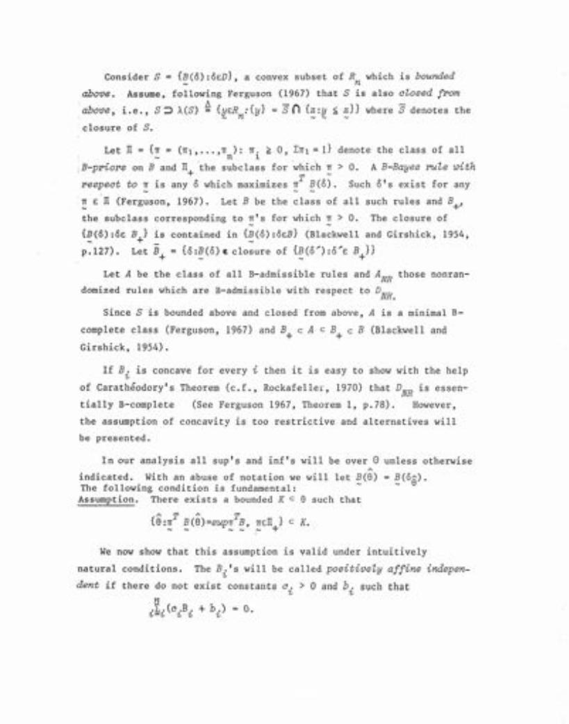
Consider S = {B(O):O£D}, a convex subset of R which is bounded_ n

above. Assume. following Ferguson (1967) that S is also closed from

above, i.e., S~ A(S) ~ {~!Rn:{Y} = Sn {z:y ~ z}} where S denotes the

,closure of S.

Let IT = {7T = (7Tl,"" 7T ): 7T. £ 0, L:7Tl = I} denote the class of all- , n ~ "

.Br-ptriore on Band II+the subclass for 'whic'h~ > O. A B-Bayes rul:e with

respect to ~ is any 8 which maximizes 7TTB(8). Such 8's exist for any

7T £ IT (Ferguson, 1967). Let B be the class of all such rules and B+~

the subclass corresponding to n's for which n > O. The closure of- -{~(O):O£ B+} is contained in {~(8):8£B} (Blackwell and Girshick, 1954,

p.127). Let B+ = {8:~(8)£ closure of {~(8~):8~!B+}}

Let A be the class of all B-admissible rules and ANR

those nonran-

domized rules which are B-admissible with respect to DNR•

Since S is bounded above and closed from above, A is a minimal B-

complete class (Ferguson, 1967) and B+ c A c B+ c B (Blackwell and

Girshick, 1954).

If Bi is concave for every i then it is easy to show with the help

of Caratheodory's

tially B-complete

Theorem (c.f., Rockafeller, 1970) that DNR is essen-

(See Ferguson 1967, Theorem 1, p.78). However,

the assumption of concavity is too restrictive and alternatives will

be presented.

In our analysis all sup's and inf's will be over 8 unless otherwiseA

indicated. With an abuse of notation we will let B(8) = B(oS)'The following condition is fundamental: --

Assumption. There exists a bounded K c 8 such that

A TAT{e:~ ~(e)=sup~~, ~!IT+} c K.

We now show that this assumption is valid under intuitively

natural conditions. The B.'s will be called positiveZy affine indepen-1-

dent if there do not exist constants c. > 0 and b. such that1- 1-

n.L.. (c .B. + b.) = o."=,, "" "

Lemma 2.1. If the B.'s are bounded, positiveLy affine independent1.

jUnctions for which there exists for every S > 0, a bounded set K c 8I A A £.

'euoh that B (8) ~ inf B + E; for every 8 tJ K iohere S is the vector whoseI - - - E.:

ielements are aZl E.:, then the Assumption holds.

.Pr oo f , Let g = rrTB. Then I;;~ inf{sup g -infg :1rEII} > O. For if noti . rr -~. rr rr -'there would exist {rrC1.») such that sup g (i) -inf g (L) 7 0 as i -+ co.

. _ C.) rr rr .Since IT is compact these exists a n 0 E IT and subsequence {rrC)} such

that' rr(j) -+ rrCO). Since the B. 's-are bounded, sup e -inf-g is con-- - 1. rr rr

tinuous in ~ so grr(o) = d, some constant, over 8. But this contradicts

the hypothesis that the B. 's are positively affine independent. So I;;1.

> 0.

Choose s <I;;and

~ s -I;; + sup[,rr.B.<1. 1.

A A

K = K. Then for 8 tJ K, Err.B.(8) ~ E.: + Err.infLrr.B.E.:. 1. 1. 1. 1. 1.

supEn.B. for all tr so the conclusion f oILows .//1. 1.

The proof of the following lemma is straightforward and hence omit-

ted.

A

Lemma 2.2. If {8:B. ~ M}, i=1, ...,m are for some M, bounded with a---- 1.

nonempty intersection, K, then the assumption holds. I I

A principal result is the following:

Theorem 2.3. If the Assumption is valid and the B. 's are ~ice1.

differentiable, DNR is essentially B-complete if and only if for every

rrsIT , the Hessian matrix of nTB is negative semi-definite at every point- + 6 A T --of E = {8:oe E ANR and ~ V ~(~) = o} UJhere V, the gradient operator, is

applied oo-ordinate-iaiee to generate rota vectors.

Proof. The necessity is obvious. To prove sufficiency note that if~8 E E, it cannot be dominated by a randomized rule. And since E has a

compact closure, the points in the closure of {rCe):e E.: E} are profiles

of elements of DNR. I I

"Essentially" cannot be dropped from the statement of the last

Theorem. It is easy to vizualize 8's for which the Hessian matrix of

Theorem 2.3 is even negative-definite at points, {a}, where ~T~,~Err+'

attain their local maxima but where the elements of the closure of

{B(a)} correspond to elements of both DNR and D -DNR·

The set E in Theorem 2.3 can be explicitly determined whenA

B. (9) = u. (b. (a) ), i = 1, ... ,n (2.1)~ ~ ~

where the b's are strictly concave and the U's are strictly increasing.A T A

Then E = {9:~ V~(~) = 0, ~!TI+}.

Example 2.1. Weerahandi and Zidek (1983) show that when a certain

class of normal posteriors and conjugate utility functions obtain,A 1 A 2

B.(9) = exp [--2QC9- 9.) ], i = 1, ...,n, in the case where p = 1 and~ ~

the preference-belief dispersion matrix is a constant, Q > O. In this

case it is easily shown that the Hessian of Err.B., i.e., Err.d2B.(9)/dez,~ ~ ~ 1

is a positive multiple of Ev.(S. - 8)2 - -21Q_1 where v. = rr.B.(8)/Err B (~ ~ . ~ ~~ r r

8) and 8 = EVi8i. Thus DNR is essentially B-complete in this example

if any only if for every ~ > 0, Ev i (8i - 8) 2 < ~Q_l., But the left hand

side of this inequality is obviously maximized over V by the achievable

choice v =v. = -21where the subscripts "max" and "min" denote indices

max m~n

at which 8i

attains a maximum and minimum respectively. Thus DNR is

essentially B-complete if and only if

(S - S . ) 2 < !Q-l .max m~n 2

(2.2)

This result generalizes for p = 1 the result of Weerhahandi and Zidek

(1983) which was for the case n = 2.

Theorem 2.3 can be difficult to apply in specific cases since this

entails the examination, in principle, of the Hessian matrix of LTI.B.~ ~

over a broad domain, for each ~ in a large class (TI+). The next theorem

would be easier to apply in the subclass of such cases which lie within

its domain of applicability. There and in the sequel d2f/dXdY will

denote the second mixed derivative of f with respect to x and y.

Theorem 2.4. Assume that A ~(d2B IdB.dB.), an (n - 1) x (n- 1) matrix,n i. J

is well defined at all points of the set E defined in the Theorem 2.3.

Then DNR is essentially B-complete if and only if A is negative semi-

definite at aLL such points.

Proof. Suppose A is positive definite at say ea 1/ E.A

Then for 8's

"close to 90•

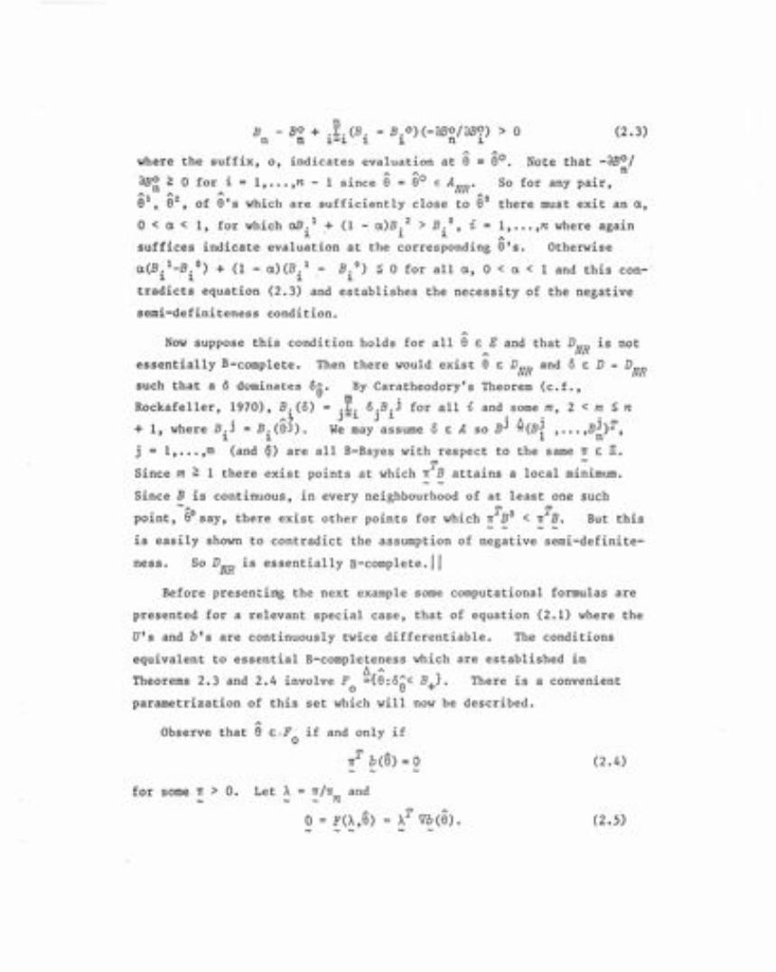
nB - BO + .~. (B. - B,O) (-8Bo/8B9) > 0n n L-L 1 L n L

where the suffix, 0, indicates evaluation at 8 = 8°.

(2.3)

aB~ ~ 0 for i = l,...,n - 1 since e = ea E ANR.

A A A A

el, e2, of 8's which are sufficiently close to eO there must exit an a,

, 1 ( )2 0' ,o < a < 1, for whLch aB, + 1 - aB. > B. , ~ = l,...,n where agalnL ' L L A

suffices indicate evaluation at the corresponding 8's.

a(B,I-B,O) + (1 - a)(B,1 - B.o) ~ 0 for all a, 0 < a < 1 and this con-'1 1 l' L

tradicts equation (2.3) and establishes the necessity of the negative

Note that -oBo/n

So for any pair,

Otherwise

semi-definiteness condition.

A

Now suppose this condition holds for all 8 E E and that DNR is notA

essentially B-complete. Then there would exist 8 E DNR and 0 E D - DNR

such that a 0 dominates 0g. By Caratheodory's Theorem (c.f.,m .

Rockafeller, 1970), B. (0) = .~. o.B.J for all i and some m, 2 < m ~ n• A~ J-L J L . 6' .

+ 1, where B.J = B.(8.]). We may assume 0 E A so BJ -(BJ1, ••• ,BJ)T,

1 1 n

j = l,.•.,m (and~) are all B-Bayes with respect to the same n E IT.

Since m ~ 1 there exist points at which nTB attains a local minimum.

Since B is continuous, in every neighbourhood of at least one such

point,-eo say, there exist other points for which nTBo < nTB. But this- - --

is easily shown to contradict the assumption of negative semi-definite-

ness. So DNR is essentially B-complete.1 I

Before presenting the next example some computational formulas are

presented for a relevant special case, that of equation (2.1) where the

U's and b's are continuously twice differentiable. The conditions

equivalent to essential B-completeness which are established in6 A

Theorems 2.3 and 2.4 involve Fa ={8:oeE B+}. There is a convenient

parametrization of this set which will now be described.

A

Observe that e E,F if and only ifo

T A

n b(8)=O- - -

(2.4)

for sornen > O. Let A = n/n and_ n

o '" F(A,e) AT Vb(f3). (2.5)

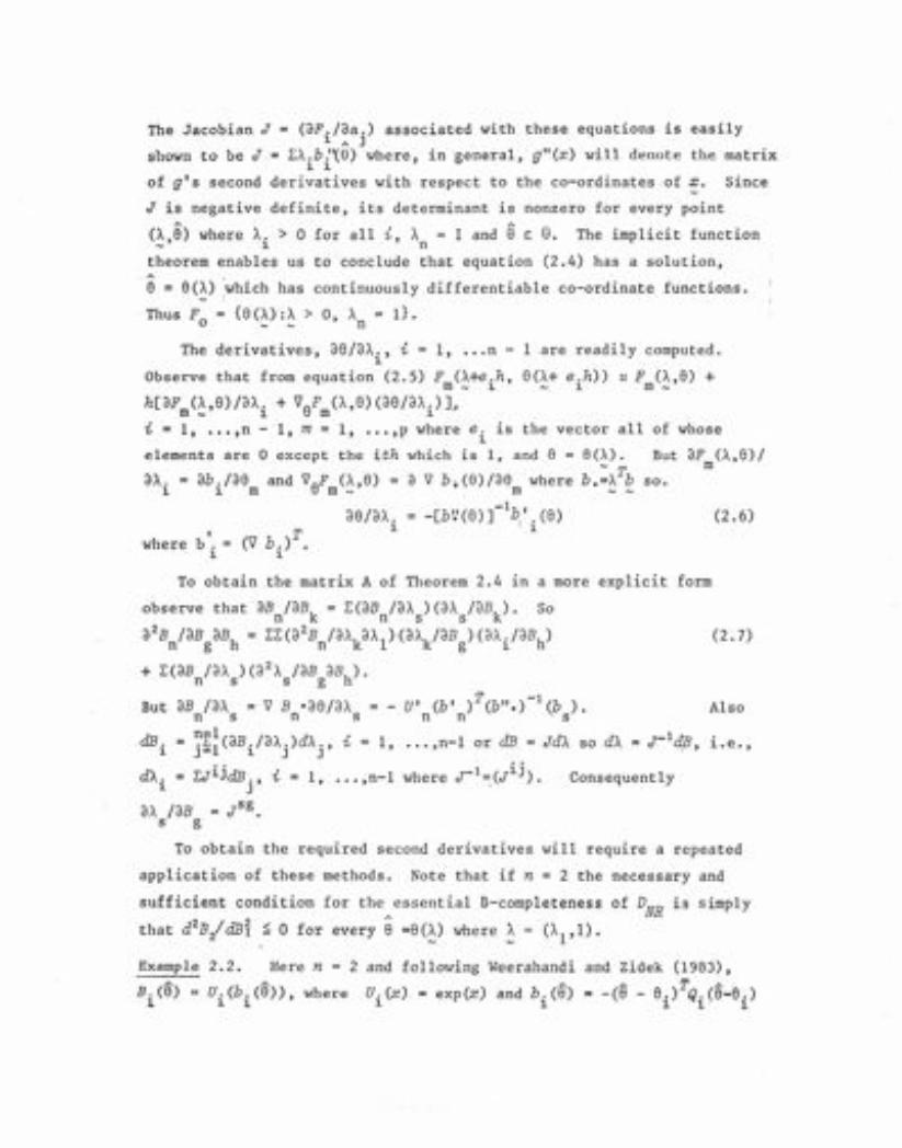
The Jacobian J = (aF./aa.) associated with these equations is easily~ A J

shown to be J = L:A.b."(O)where, in general, g"(x) will denote the matrix~ 1

of g's second derivatives with respect to the co-ordinates of~. Since

J is negative definite, its determinant is nonzero for every point

(A,6) where A. > 0 for all i, A = I and e e: e. The implicit function. - L n

theorem enables us to conclude that equation (2.4) has a solution,

e = e(A) 'which has continuously differentiable co-ordinate functions.- ,

Thus Fo = {S(A):A > 0, A = I}._ _ n

The derivatives, ae/aA., i = 1, ...n - 1 are readily computed.1

Observe that from equation (2.5) F (A+e.h, 8(1.+ e.h» ~ F (A,S) +m _ 1 - 1 m _

h[aF (A,8)/oA. + ~eF (A,e)(oe/oA.)]~m _ 1 m ~

i = 1, .••,n - 1, m = 1, •..,p where e. is the vector all of whose1.

elements are 0 except the ith which is I, and S = SeA).- T

ab./as and ~eF (1.,8) = a ~ b~(8)/aS where b.=A b so.1 m m - m - -

-lboe/oA. = -[b~(e)] .'.(e)

1 . 1

But aF (A,8)1m

aA.1

(2.6), T

where b . = (~ b.) .1 1

To obtain the matrix A of Theorem 2.4 in a more explicit form

observe that aB laBk = L:(oB /01. )(oA /aBk)' Son n s s

02Bn/aBgoBh = EE(02Bn/oAkOAl) (aAk/oBg) (oAi/oBh) (2.7)

+ E(aB /oA )(021. loB oBh).

n s s g

But oB /OA = ~ B -aa/ax = - u' (b' )T(b".)-l (b ). Alson s n s n n . s

dB. = ~E11(aB.loA.)dA., i = 1, ...,n-1 or dB = JdA so dA = J-1dB, l.e.,1 J= i. J J '

• • 1 ijdA. = EJ1JdB., i = 1, ...,n-1 where J- =(J). Consequently1 J '

ax /aB = Jsg•s g

To obtain the required second derivatives will require a repeated

application of these methods. Note that if n = 2 the necessary and

sufficient condition for the essential B-completeness of DNR is simply

that d2B2/dB~ ~ 0 for every 8 =e(~) where ~ = (AI,l).

Example 2.2. Here n = 2 and following Weerahandi and Zidek (1983),A A ~ A T A

B.(S) = V.(h.(S», where V.(x) = exp(x) and b. (8) = -(8 - e.) Q.(e-8.)1 1 1 1 11 1 1

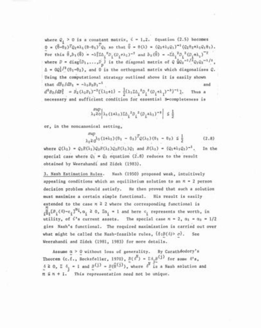
where Q. > 0 is a constant matrix, i~ 1 T A

o = C8-82)TQ2+AIC8-el) Ql so that e =~ ~ ~ ~ 2

For this e,bl(B) = -A1L6. D.(D.+A1)-1. 1. 1.

;where D = diag{D1, •.. ,D } is the di'agonal. / p.11= OQ~ ,~(81-82)' and 0 is the orthogonal matrix which d iagona lLzes Q.

Using the computational strategy outlined above it is easily shown

'H 1that d1:J2/dB1 = -A1B2B1- ,

2 2 ' '2 '{ } 1{ 2 2 3} 1d B2/dBl = B2(AIB1)- [1..1+1 - -2 AILI1.D. eD.+A1)- - J. Thus a

.. . .11. 1. 'necessary and suf fi.cient condition for essential B-completeness is

1,2. Equation (2.5) b~comes

e(A) = (Q2+>I.lQ1)-I(Q'L8'L+A.IQ1e1)'

~ "2 2 '-2'and bz(9) = -"i.6. D. (D.+A

I)

1. 1 1.

matrix of Q ~Q'2.-1 /2Ql Q'2.'-1 /,Z ,

and

sup I I'2. 2 3AI~OIAI~1+A1~Ll1i Di (Di+Al)-

< 1= 2

or, in the noncanonical setting,

sup TA ~OAl(1+>"1)(81 - 82) Q(Al)Ce11 , ,

where Q(A1) = QIR(Al)Q2R(Al )Q2R(>"dQl and R(Al)

1- e2) ~ 2

(Ql+AlQ'2.)_l.

(2.8)

In the

special case where Ql :;;Q2 equation (i.8) reduces to the result

obtained by Weerahandi and Zidek (1983).

3. Nash Estimation Rules. Nash (1950) proposed weak, intuitively

appealing conditions which an equilibrium solution to an n = 2 person

decision problem should satisfy. He then proved that such a solution

must maximize a certain simple functional. His result is easily

extended to the case n ~ 2 where the corresponding functional isn a'.lll[B.(o)-c.] 1,a. ~ 0, La. = 1 and here c. represents the worth, 1.n1= 1. 1 1 1 1.

utility, of i's current assets. The special case n = 2, a1 = a2 = 1/2

g1es Nash's functional. The required maximization is carried out over

what might be called the Nash-feasible rules, {8:B(8» c}. See

Weerahandi and Zidek (1981, 1983) for more details.

Assume a > 0 without loss of generality. By Caratheodory's

Theorem (c.f., ~ocksfeller, 1970), BCdV) = E8.Bej) for some 8's,

o ~ 0, L o. = 1 and B(j) = B(S(j»,-where aN f~ a Nash solution and- J --m ~ n + 1. This representation need not be unique.

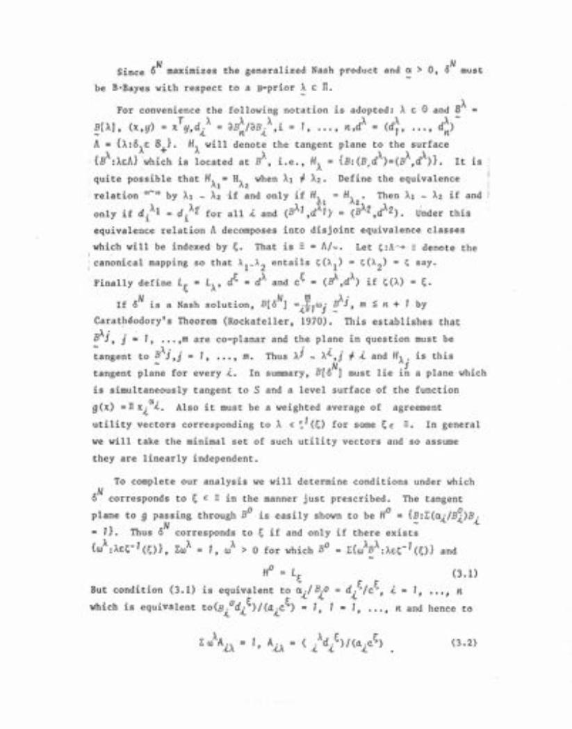
Since oN maximizes the generalized Nash product and a > 0, oN must

be B-Bayes with respect to a B-prior A s n.

For convenience the following notation is adopted: A ! G and BA

BrA], (x,!!) = xT!!,d.A = 'dBA/'dB.\i = 1, ... , n,dA = (dA1, ... , dA)-_ .{. n.{. n

A = {A:(\E:B+}. HA will denote the tangent plane to the surface

;{BA:AE:A}'which is located at BA, i.e., HA = {B:(B,dA)=(BA,dA)}. It 1S

;quite possible that HA1

= HA2 when Al f A2. Define the equivalence

·relation"-" by Al - A2 if and only if H~ = HA' Then Al - A2 if and

·only if d.AI = d.A'l.for all -<.. and (BAl ,d ~).= (~A'l.,dA'l.).Under this1 l.

equivalence relation A decomposes into disjoint equivalence classes

which will be indexed by I;. That is == = 11./-. Let l;:A-~-+ :: denote the

i canonical mapping so that Al-A2

entails seAl) = S(A2) = S say.

·Finally define L~ = LA' d~ = dA

and e~ = CEf,dA) if sCA) = ~.

N N m x .If 8 is a Nash solution, B[8 ] ='~IWj' B'}, m ~ n + 1 by

.{.- -Caratheodory's Theorem (Rockafeller, 1970). This establishes that

A' .'B J, j = 1, ... ,m are- A. •

tangent to ~ },j = 1,

co-planar and the plane

j .i ,... ,m. Thus A -/\,j

tangent plane for every -<... In summary, BlaN]

in question must be

f -<.. and HA' is this. . j .

must 11e 1n a plane wh1ch

is simultaneously tangent to S and a level surface of the function

g(x) =IT xioi. Also it must be a weighted average of agreement

utility vectors corresponding to A E ;1(~) for some ~E ==. In general

we will take the minimal set of such utility vectors and so assume

they are linearly independent.

But condition (3.1)

To complete our analysis we will determine conditions under which

oN corresponds to S E == in the manner just prescribed. The tangent

plane to 9 passing through BO is easily shown to be HO = {B:E(a-<../Bi)B.

= I}. Thus oN corresponds to S if and only if there exist; .{.

{wA:A!~-1 (s)}, EwA = 1, wA> 0 for which BO = E{wABA:A!~-1 (s)} and

°H = L~ (3.1)

is equivalent to a./B.O = d.~/e~, -<.. = I, .." n~ ~ A.. A.. A...

to(B.odj )/(a.c ) = 1, 1 = I, ... , n and hence toA.. ~ .{.. .

which is equivalent

AA -E W ix : 1 A.,, .{./\

le s ~= ( . d. ) / (o...c. )-<- -<- -<-

(3.2)

~1Let A = (A,,) = (A ,

, ..LI\

Then equations (3.2) may

...,A T

A m) :: (A1, ..., T T

A) where mYl.

Is-1(01.be written as

A A T~w A = l: = (1, "', 1)

-Yl. '(3.3)

or ~lternatively

Aw = Z

'Thus oN corresponds to ~ if and OnlY-~f there exists w ~WA

wA > 0 for which equations (3.3) and (3.4) hold.

Equation (3.3) shows that ~ must be in the cone of {AA" "', AAml

,If, for example, m = 1, this C~:dition shows that 8N = 8

Aif and only

if B,A(dBA/dB,A) = a,~A(8BA/aB~). Equation (3.4) implies that.{. T Yl.1 r: .{.j n j

w = (A A)- A ~ which implies that unless the quantity on the right

hand side of ::uation (3.4) satisfies ~ T(ATA)-'ATZ = 1 and has non-N _m -Yl.

negative coordinates, 8 cannot have s-'(~) as its support. Converse-

ly, if these conditions are satisfied 8N

does correspond to ~.

(3.4)

1 ,

In general this characterization may be difficult to apply because

the equivalent classes, s-1 (~), are too numerous to be explicitly

determined. For small values of Yl., however, this characterization 1S

applicable. We illustrate this in the following example.

Example 3.

taking p = Yl.

The set S is

Consider the specializationT

= Z ,Q, = 12, QZ = 12/2, 8,

illustrated in Figure 3.1.

of Example 2.2 obtained byT

= (0,0) and 82 = (1,1.5).

Figure 3.1 ,Here

It is clear from Figure 3.1 that there is just a single ~ for which

~-1(~) contains more than one point, namely that for which s-l(s) =

{A1,A2}. Whether or not oN has support determined by this class

depends on a1

and aZ'

We first determine a1

and a2 by graphical analysis. [For the

details see de Waal et aI, 1982]. The result is 1..1 =(0.2135,0.3203)T.

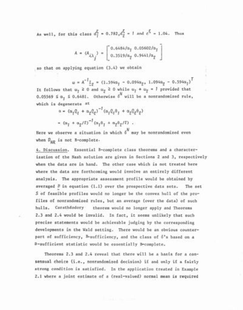
As well, for this class dJ = 0.782,d~ = t and c-t"= 1.04. Thus

-O.6484f~1 O.05602f~1 J

A = (A. ) =~Aj I 0.35l9/a

Z0.944l/aZ

so that on applying equation (3.4) we obtain

-1 )TW = A ~Z = (1.594a

t- 0.094aZ' 1.094a2 - 0.594a

1

It follows that wl~ 0 and w

2~ 0 while w

t+ Wz = 1 provided that

0.05569 ~ at ~ 0.6481. Otherwise oN will be a nonrandomized rule,

which is degenerate at-1

Cl = (a1Ql + aZQZ) (atQt8l + aZQZ8Z)

-1= (a

1+ aZ/Z) (a

18l+ a

Z8Z/2)

Here we observe a situation in which oN may be nonrandomized even

when VNR

is not B-complete.

4. Discussion. Essential B--complete class theorems and a character-

ization of the Nash solution are given in Sections 2 and 3, respectively

when the data are in hand. The other case which is not treated here

where the data are forthcoming would involve an entirely different

analysis. The appropriate assessment profile would be obtained by

averaged B in equation (1.1) over the prospective data sets. The set

S of feasible profiles would no longer be the convex hull of the pro-

files of nonrandomized rules, but an average (over the data) of such

hulls. Carath~odory theorem would no longer apply and Theorems

2.3 and 2.4 would be invalid. In fact, it seems unlikely that such

precise statements would be achievable judging by the corresponding

developments in the Wald setting. There would be an obvious counter-

part of sufficiency, B-sufficiency, and the class of o's based on a

B-sufficient statistic would be essentially B-complete.

Theorems 2.3 and 2.4 reveal that there will be a basis for a con-

sensual choice (i.e., nonrandomized decision) if and only if a fairly

strong condition is satisfied. In the application treated in Example

2.1 where a joint estimate of a (real-valued) normal mean is required

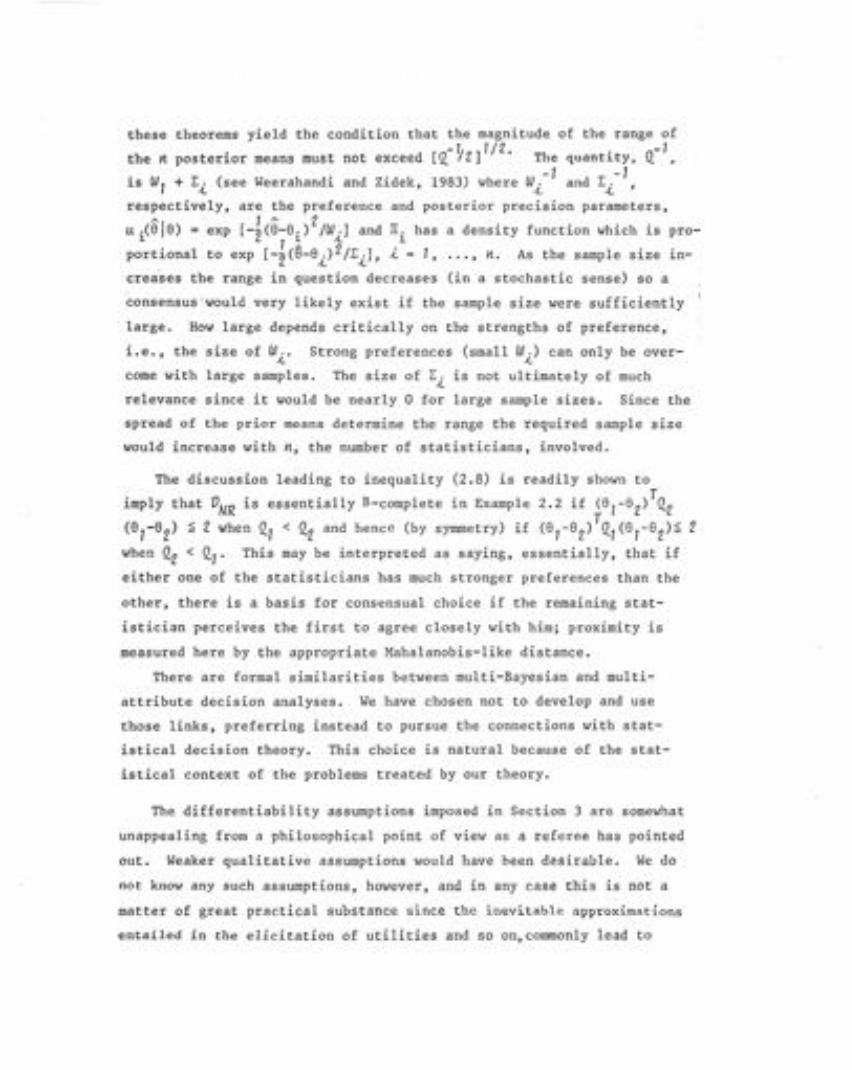
these theorems yield the condition that the magnitude of the range of

• [n-1Il ]1/2. . Q-lthe n posterlor means must not exceed ~ I . The quant1ty. .'

is W1 + E. (see Weerahandi and Zidek, 1983) where W.-7 and E.-1,..{. ..{. ..{.

respectively, are the preference and posterior precision parameters,

U .(8/8) = exp [--21 (8-8.)2/W.J and IT. has a density function which is pro-1 . 1 1..{. 1

portional.to exp [--Z(g-e.)2/E.J, i = 1, ... , n. As the sample size 1n-. ..{. ..{.

crea~es the range in question decreases (in a stochastic sense) so a

~onsensus:would very likely exist if the sample size were sufficiently

large. How large depends critically on the strengths of preference,

i.e., the size of W .. Strong preferences (small W.) can only be over-..{. ..{.

come with large samples. The size of E. is not ultimately of much..{.

relevance since it would be nearly 0 for large sample sizes. Since the

spread of the prior means determine the range the required sample S1ze

would increase with n, the number of statisticians, involved.

The discussion leading to inequality (2.8) is readily shown to

imply that VNR

is essentially B-complete in Example 2.2 if (81-82)TQ2

(87-82) ~ 2 when Q.7 < Q.2 and hence (by symmetry) if (el-e2)TQl(el-82)~ 2

when QZ < Q.1· This may be interpreted as saying, essentially, that if

either one of the statisticians has much stronger preferences than the

other, there is a basis for consensual choice if the remaining stat-

istician perceives the first to agree closely with him; proximity 1S

measured here by the appropriate Mahalanobis-like distance.

There are formal similarities between multi-Bayesian and multi-

attribute decision analyses. We have chosen not to develop and use

those links, preferring instead to pursue the connections with stat-

istical decision theory. This choice is natural because of the stat-

istical context of the problems treated by our theory.

The differentiability assumptions imposed in Section 3 are somewhat

unappealing from a philosophical point of view as a referee has pointed

out. Weaker qualitative assumptions would have been desirable. We do

not know any such assumptions, however, and in any case this is not a

matter of great practical substance since the inevitable approximations

entailed in the elicitation of utilities and so on,commonly lead to

choices which are made from parametric classes of convenient, smooth

models.

Acknowledgement. This work was supported by the University of the

Orange Free State, South Africa, and the Council for Scientific and

Industrial Research, where the last author was a Visiting Scientist

while on leave from the University of British Columbia. This leave

was financed in part in Canada's Research Councils for the natural

sciences and engineering and for the social sciences and humanities.

The work benefitted from the comments of Dr. Theo Stewart.

References

[1] Berger, J.O. (1980). Statistical decision theory. New York.

Springer-Ver1ag.

[2] Berger, J.O. (1982). The robust Bayesian viewpoint. Tech. Rep.

82-9, Dept. of Statistics, Purdue University.

[3] B1ackwell, D. and Girschick, M.A. (1954). Theory of games and

statisical decisions. New York. John Wiley and Sons Inc.

[4] De Waal, D.J., Groenewald, P.C.N., Van Zy1, J.M., Zidek, J.V.

(1982). A randomized solution for mu1ti-Bayes estimates of the

mu1tinormal mean. Unpublished manuscript.

[5] Ferguson, T.S. (1967).

theoretical approach.

Mathematical statistics: a decision

New York. Academic Press.

[6] Morris, C.N. (1983). Parametric empirical Bayes inference:

theory and applications. ~. Amer. Statist. Assoc., 78:47-65.

[7] Nash, J.R. Jr. (1960) The bargaining problem. Econometrica,

18:155-162.

[8] Rockafellar, R.T. (1970) Convex Analysis. Princeton University

Press.

[9] Weerahandi, S. and Zidek, J.V. (1981). Multi-Bayesian statistical

decision theory. J. Roy. Statist. Soc., Ser.A. 144:85-93.

(10) Weerahandi, S. and Zidek, J.V. (1983). Elements of multi-

Bayesian decision theory. Ann. Statist., 11.

[11] Yu, P.L. (1973). Introduction to domination structures in

multicriteria decision problems. In: J.L. Cochrane and

Zeleny, Eds., Multiple Criteria Decision Making. South

Carolina Press, pp. 249-261.

If(l!?1Jltr.}1T()H1)l)1U-;rt'1111l0J./l):;''llj'1.'1JfI!,q1)1.'09

(28,18)<;"'.,,?1.\-[Iij"!"7!?71l)2"Q?'<;'llo790:ray0lJl