Embed Size (px)
Citation preview

MULTI-AXIS NUMERICAL CONTROL
A thesis submitted for the degree of
Master of Engineering
in the
University of Canterbury
New Zealand
by Ma Li
1989

ACKNOWLEDGEMENTS
I am indebted to my supervisor Dr G R Dunlop for his guidance, encouragement and
help during the course of this research and preparation for this thesis. I am grateful to
Mr N Bolland for his sincere concern and help.
I wish especially to present this to my husband Xiao Xuan, for his strong
encouragement and support, and to all of my family for their significant help.
Finally. my thanks go to all those who assisted me in many ways with their
knowledge, time and enthusiasm.
I

II
CONTENTS
ACKNOWLEDGEMENTS I
ABSTRACT IV
PUBLISHED PAPERS V
LIST OF SYMBOLS VI
CHAPTER 1 INTRODUCTION 1
1.1 Robotics 2
1.2 Satellite Tracking - The "Key Hole" Problem 3
1.3 The Stewart Platform 5
CHAPTER 2 NUMERICAL CONTROL OF MULTI-AXIS MACHINERY 13
2.1 Introduction 13
2.2 Single Motor Control Problem 14
2.3 Multiple Motor Control Problem 17
2.4 Accurate Multiple Motor Control 18
CHAPTER 3 DESIGN OF A MULTI-MOTOR CONTROLLER 26
3.1 Introduction 26
3.2 The Computer and Its I/O Channel 27
3.3 The HCTL-lOOO 28
3.3.1 The Operation 28
3.3.2 User Accessible Registers 29
3.3.3 Timing Diagram 30
3.4 Design of the Controller 31
3.4.1 IBM-PC I/O Bus 31
3.4.2 Decoder and Control Logic 31
3.4.2.1 Clock 31
3.4.2.2 Control Signals Decoding 32
3.4.2.3 Data Transfer 33
3.4.2.4 An Example 33
3.4.3 Reset 33
3.4.4 HCTL-1000 34
3.4.5 Buffer 35
3.4.6 Controller Socket 35
3.5 Testing 35
CHAPTER 4 DC MOTOR PWM SERVO DRIVE 51
4.1 Introduction 51

III
4.2 DC Motor 52
4.2.1 Operation Principles 52
4.2.2 Classification and Characteristics 53
4.2.2.1 Shunt Motor 54
4.2.2.2 Series Motor 54
4.2.2.3 Compound Motor 55
4.2.2.4 Separately Excited Motor 55
4.2.2.5 Constant Field and Permanent Magnetic DC Motors 55
4.2.2.6 Motor Parameters
4.3 DC Motor PWM SeIVo Drive
4.3.1 Introduction
57
58
58 4.3.2 Three Modes of PWM Drives 59
4.4 Design and Testing 59
4.4.1 Bipolar PWM SeIVo Drive 59
4.4.1.1 Logic Design 59
4.4.1. 2 PWM Drive Design 61
4.4.1.3 Problem and Analysis 62
4.4.2 Limited Unipolar PWM SeIVo Drive 62
4.4.3 Motor Performance 63
4.5 SUITllDary 64
CHAPTER 5 SYSTEM MODELLING AND ANALYSIS 82
5.1 Control Modes 82
5.1.1 Position Control 82
5.1.2 Proportional Velocity Control 83
5.1.3 Integral Velocity Control 84
1.4 Trapezoidal Profile Control 84
5.2 The Electromechanical Model 85
5.2.1 The Motor 85
5.2.2 The Encoder 87
5.2.3 The Control System Modelling 88
5.2.4 Theoretical Response 91
5.3 Experimental Response Analysis 92
5.4 SUITllDary 93
CHAPTER 6 CONCLUSION 105
APPENDIX A SYSTEM PERFORMANCE FOR LARGE STEP INPUTS 107
APPENDIX B ANALYSIS OF FRICTION EFFECTS 109
APPENDIX C PROGRAM LISTING 113
REFERENCES 123

ABSTRACT
This thesis presents the analysis, design and development of a multi-axis machinery
numerical control system. The purpose of this research is to provide a numerical
control method to overcome the multi-axis numerical control problem.
The control system includes an IBM-PC computer as a host processor, a plug in multi
motor controller board based on commercial numerical motor controller ICs. These
implement a software specified digital control algorithm and output a PWM control
number. Six motors, their driven actuators, and digital incremental feedback encoders
complete the system.
IV
The experimental aspects of the work included the design of the IBM-PC plug in motor
controller board and the motor drive board, computer software for real-time control
and the system testing. For the theoretical aspects of the work, control theory was
used to develop the mathematical model of the system. This aimed at providing a tool
to predict and optimize the system performance, therefore, to fulfill the high
positioning and high precision control task.

PUBLISHED PAPERS
Dunlop GRand Ma Li: Multi-axis Numerical Control. Proc. IMC Conf.,
Christchurch, New Zealand, May 1988
Mzulpurkar N V. Ma Li, Dunlop GRand Johnson G R: Design of Parallel Link
Robot. Proc. NELCON Conf., Christchurch, New Zealand, August 1988
v

Az
El
T(f) T i (f)
J e(t)
d
T1
T2
0)1
0)6
Tm <1>
Ia
JS, E
0)
Ra
Vm Kt
Ke
Pm Pe
Vs lAB
Ion
y. ill
t
dO) dt K m
90· - $, azimuth
90° - e, elevation
LIST OF SYMBOLS
(step motor) pull-out torque at a stepping rate f load torque
motor inertia
rotating angle of motor shaft
microprocessor direct control delay value time taken in the idle path (microprocessor direct control)
time taken in the step path (microprocessor direct control)
motor velocity in one motor direct control
motor velocity in one motor direct control
motor shaft torque
DC motor magnetic flux per pole
motor armature current
constant of the motor winding
motor back emf voltage
motor shaft velocity
motor armature resistance
motor terminal voltage
motor torque constant
motor back emf voltage constant
mechanically developed motor power
electrical power absorbed in the motor rotor
the voltage of the power supply the current flowing through the motor in PWM servo drive
the current flowing through the motor during the FETs "on" time in PWM
servo drive the current flowing through the motor during the FETs "off' time in PWM
servo drive PWM servo drive input voltage
time
motor shaft angular acceleration
the motor constant
VI

K
A
B
T
Av Tfr
Vef
a Kex
Kth
PWM%
the motor time constant
the gain number in the register R22H in the HCTL-lOOO
the zero number in the register R20H in the HCTL-IOOO
the pole number in the register R21H in the HCTL-lOOO
sample time amplitude of a step input
torque caused by friction
the effective voltage
the effective voltage coefficient
the slope of the experimental response
the slope of the theoretical response
the PWM duty cycle
VII

1
CHAPTER 1
INTRODUCTION
Despite rapid developments in electronics and communications, traditional mechanical
engineering is still an essential part of modern society. In particular, Multi-axis
machinery is an important field which draws on all of these engineering disciplines.
Multi-axis machinery is a type of machinery which has multiple axes or mechanisms,
each of which can execute a required motion to produce a coordinated motion for the
whole machine. The purpose of this type of machine is to do complicated jobs so as to
increase efficiency or reduce costs. Robots, satellite tracking mechanisms and some
machine tools are typical applications of such machines.
The remaining part of this chapter will discuss these applications including their
functions and existing problems, and then give a mechanism as a solution. The second
chapter discusses the numerical control problems associated with ordinary control
means used to drive multi-axis machinery. A satisfactory solution to these problems is
developed.
The later chapters present the design, theoretical analysis and performance of a multi
axis machine numerical controlleI," developed during this research, i.e. the problems
raised in CHAPTERs 1 and 2 will be solved.

2
1.1 ROBOTICS
Since the word "robot" was first introduced in 1917 (McCloy 1986), it has become
widely used by many people. Because of the potential shown by robots in substituting
people's labour especially in dangerous or boring work, the use of robots is becoming
widespread.
According to mechanical arrangement of the manipulators, robots can be divided into
two categories: i) The serial or open link manipulators and ii) the parallel or closed link
manipulators.
The arrangement of a six degrees of freedom serial link robot is shown in Fig. 1.1. It
has six fixed length links and is a traditional type coming from the simulation of the
human body, i.e. anthropomorphic. Each link can swing through an arc with respect
to the preceding link. Hence, the manipulator has six degrees of freedom and the end
effector (or gripper) is positioned within the working volume.
The main advantages of a serial link manipulator are:
-the manipulator has high mobility, Le., has a long reach and a large range of
motion since the links are connected one after another;
-it has flexible reaching points, even to corners.
The disadvantages are:
-the cantilever construction subjects the manipulator to large bending moments,
which results in link deflections at full reach. This decreases the accuracy of
positioning and limit the application under heavy loads;

3
-a given set of end actuator coordinates does not have a unique set of joint
coordinates. In other words, the link positions are usually indeterminate (c.f. Fig.
1.2) (Dunlop & Afzulpurkar 1988).
1.2 SATELLITE TRACKING - THE "KEY HOLE" PROBLEM
Satellites are now the dominant carriers of telecommunications and are playing
important parts in space and the earth resource exploitation. Satellite tracking systems
have been developed since 1963 after the space research started in late fifties. Good
tracking systems must be able to find their satellites quickly and maintain
. communication with them through unexpected orbital changes. For maritime earth
stations, they need also be able to overcome the effect of rolling and pitching of the
ships. The earth station antenna dish diameters may be as large as 30m and can weigh
up to several hundred tons (Afzulpurkar et al 1988). As the frequency used increases,
the beamwidth is reduced, so more than a fraction of a degree of apparent satellite
movement must be tracked (Pratt and Bostian 1986). Hence a good tracking
mechanism is required to ensure the completion of the task On the other hand, they
must be relatively inexpensive.
The present popularly used tracking mechanisms can be generally divided into three
categories: Alt-Azimuth or Az-El mount (c.f. Fig. 1.3), X-Y mount (c.f. Fig. 1.4) and
a combination of these two (c.f. Fig. 1.5 and Miya 1981).
The path followed by any satellite moving around the earth is a decaying ellipse in the
orbital plane. The coordinates to which the antenna must be pointed to communicate
with the satellite are called the "look angles". These are most commonly specified as
"azimuth" (Az) and "elevation" (El). Azimuth (90" - l/> ) is measured eastward from

4
geographic north to the intersection of the satellite orbital plane on the horizontal plane
at the earth station. Elevation (900
- e ) is the angle measured above the horizontal
plane to the line of sight of the satellite (c.f. Fig. 1.6).
An Az-El type of mounting system has two axes, Az and El. The antenna bore sight
axis will trace a semicircle on a vertical plane about El axis and can sweep a horizontal
circle about Az axis. When a satellite starts approaching to the zenith, Le. the El angle
90° (c.f. Fig. 1.7(a», the antenna dish has to rotate the azimuth angle through 180'"
about the bore sight axis to continue the tracking because of limitations in the
mechanism (c.f. Fig. 1.7(b». Thus the system has a singularity at the zenith. During
the time taken for this 1800 azimuth rotation, the satellite moves out of the beam of a
high gain antenna and the station loses contact with the satellite. This is known as the
"key hole" problem. The problem becomes particularly severe when the tracking
system is mounted on a ship. The rolling and pitching action of a ship causes the
singularity of the Az-El mount to trace out a flattened cone about the zenith. If the
satellite is within this flattened cone region, communication contact can be lost and the
tracking ceases. When receiving signals from deep space probes, there is only one·
chance of capturing the data sent by the space craft and such a loss of contact is
unacceptable (Afzulpurkar et alI988).
An X-Y type of mounting system has X and Y axes (c.f. Fig. 1.4). When the antenna
dish tracks a satellite along the horizontal plane and near the axis mountings, the
track in path is occluded by the mountings, so it has to rotate 180· for continuing the
tracking. Thus the "key hole" problem exists along the horizontal axis in an X-Y
mounting system. For overcoming the effect of rolling and pitching of a ship mounted
application, the antenna being able to point below the horizon is needed, so the X-Y
mounting is incapable of fulfilling this kind of tracking requirements. To solve the

5
"key hole" problem for deep space work, two ground based X-Y mounted antennas
are mounted perpendicular to each other. Thus the singularity of each antenna is
covered by the other and the signals are received and complementary mutually.
However, the cost of the tracking system is doubled.
The conventional solution to the "key hole" problem is to use a combined mount of X
Y type and Az-El type (c.f. Fig. 1.5(c) and Miya). A horizontal plane is always
maintained against ship's motions by controlling the X and Y axes of the plane. The
direction to the satellite is produced by controlling the azimuth-elevation axes mounted
on this horizontal plane. Controlling of the X-Y and Az-El axes is independent, but
the cost and complexity of the operation are greatly increased.
1,3 THE STEWART PLATFORM
The solution to the above problems in robotics and satellite tracking systems is to use a
Stewart platform mechanism (c.f. Fig. 1.8).
The Stewart platform was proposed in 1965 (Stewart) and is widely used for aircraft
simulation and other purposes nowadays. It is a parallel1ink manipulator. It consists
of two bodies connected by six legs. One body is called the base, which is usually
fixed, and the other is called the platform which is movable. Each of the legs is in the
form of a linear actuator. Each actuator has one end joined to the base and the other
end joined to the platfonn. The actuators are prismatic joints and can expand and
contract independently thus positioning the platfonn in space. This arrangement
provides a sturdy mechanism with six degrees of freedom which means it can take any

6
position and any orientation within a certain work volume. The arrangement of the
structure is symmetric to achieve maximum stiffness.
With this rigid mechanism, the joint deflection problem in serial link robotics is
considerably reduced and high accuracy positioning can be achieved. These properties
make it suitable for use in heavy duty environments, such as automotive assembly
applications and the like (c.f. Fig. 1.9).
For the satellite tracking application, an antenna dish is mounted on the platform and a
tracking system with six degrees of freedom is formed. The antenna dish can even
point 30° below the horizon with carefully designed joints (c.f. Afzulpurkar et al
1988). When this mechanism is applied in a ship mounted environment, it is able to
track the satellite rapidly without mechanism singularity limitations, therefore is a
rather simple and reliable mechanism to overcome the "key hole" problem (c.f. Fig.
L 10). The six identical actuators simplify the manufacture.
So far the solution to the problem raised in 1.1 and 1.2 has been clearly given - the
Stewart platform.

Fig. 1.1 Typical se~iel link manipulator with six degree of freedom
"'1----'--( /'" 0
Fig. 1.2 Kinematic independency in open link manipulator
7

E\
~Az
z
\
East
x
North
y
8
Fig. 1.3 Az-El antenna mount system.
2 axes
Fig. 1.4 X-Y antenna mount system.
2 axes
Fig. 1.6 Look angles

Cross-
E\
~Az
x
(a) Az, El, eros Plount. 3 axes
(b) X-Y-Y' mount 3 axes
(c) X-Y and Az-El 4 axes
. 1.5 Antenna mixed mount systems
9

Elevation axis
sight axis
axis
Fig. L 7 (a) 11.1 t-Azimuth antenna mount
Singularity position -i- . E1 = 90°
, " . . . .
Azimuth axis
Fig. 1.7(b) Singularity position of Alt-Azimuth antenna mount
10

Fig. 1.8 The Stewart platform in the project
11

Fig. 1.9 Parallel robotic based on Stewart platform
Fig. 1.10 Satellite tracking system based on stewart platform
12

CHAPTER 2
NUMERICAL CONTROL OF MULTI-AXIS MACHINERY
2.1 INTRODUCTION
Some method is required for controlling and positioning the Stewart platform or any
other multi-axis machinery. The six actuators of the Stewart platform are driven each
by a DC motor. The numerical control system discussed here is not confined only to
DC motors, but can be extended to other driving components like DC brushless
motors, step motors and hydraulic cylinders. A general discussion about the numerical
control to multiple axis machinery in a broader sense will be given.
13
Hydraulic cylinders and DC motors can use the same type of control signal Le. a
voltage or a PWM signal. Step motors require precise phase switching information
and some form of current or voltage controL Brushless DC motor can be treated as a
class of step motor.
To control these motors or hydraulic cylinders, a microprocessor is a good choice
because of its low cost and high reliabilities. However, the relatively slow speed of
most microprocessors results in limited control for more than one motor/actuator. The
various features are analyzed in following sections.

2.2 SINGLE MOTOR CONTROL PROBLEM
Take a step motor directly controlled by a microprocessor software timing as an
example, where several features must be considered. The typical pull-out torque/speed
characteristics of a step motor are shown in Fig. 2.1. This represents the maximum
torque which the motor can develop at each operating speed. If the load torque
exceeds the pull-out torque, the rotor is pulled out of synchronism with the magnetic
field and the motor stalls or even reverses. However, for velocity profiling operations,
timing is critical, more factors have to be considered. Fig. 2.2 shows the relationship
between pull-out torque and load torque. It can also be algebraically expressed as
follows (Acarnley 1982):
Where, T(f) - the pull-out torque at a stepping rate f;
T 1 (f) - the load torque;
J - the whole system inertia;
8(t) - the rotating angle of the motor.
(2.1)
14
That means, to move the load and change its velocity at the required rate, the being
developed torque of the motor must be large enough to overcome the load torque and
accelerates the system inertia, thus to keep the consistent accuracy and stability, which
are the essential requirements in step motor control. Otherwise, the motor either fails
to operate at all or drops out of step during acceleration and deceleration, causing
permanent errors (Acarnley 1982; Dunlop 1986).
To perform each specified movement during a microprocessor software direct control,
the step rate (steps/sec) and the target distance in steps are calculated. The latter one

15
can be calculated by knowing the step length. The former one can be obtained from
the following method based on the one of Acamley (1982).
The flowchart shown in Fig. 2.3 is the method giving the step interval by software for
direct control of one motor. At regular step intervals, the microprocessor software
produces a phase on/off pattern and sends it to the step motor phase switches. The
step interval can be calculated from the following:
Step Interval = dT 1 + T 2
Where, T 1 - the time taken to go through the idle path;
T 2 - the time taken to go through the step path;
d - delay value.
(2.2)
The step interval delay value d is placed in a loop counter initially, then the step interval
is established by decrementing the counter and producing a new phase on/off pattern
each time the loop counter reaches zero. Note that the loop takes typically lOllS per
loop cycle going through the idle path except on the last cycle which takes a typical
extra 50lls going through the step path. The addition of "DelayS" is to keep the time
taken in step path a constant no matter whether or not a new table is set up. The
"DelayL" here can be zero and must be increased in multiple motor control which is
discussed in the next section. Then the stepping rate can be calculated by the follo\\ring:
1 Step Rate (steps/sec) = Step Interval (sec/step) (2.3)
The timing quantization is introduced by this microprocessor software loop. The effect
on performance is illustrated by the calculated results given in Table 2.1 (Dunlop and
Ma 1988). Note that:

1) The maximum speed a motor can achieve may be limited by the operating speed
of the microprocessor to less than theone determined by the load.
16
2) At high step rates, the velocity changes (or acceleration) which must occur within
one step time (so as to maintain synchronism) are very large. For every 10 times
increase of the speed, the required acceleration increases 1,000 times. In other words,
a large torque is required to achieve large speed change when the speed is high; while a
small torque is required to achieve small speed change when the speed is low.
Nevertheless, this is contrary to the pUll-out torque/speed characteristic of a step
motor. That is, the torque T(f) available from the motor is greatly reduced when the
acceleration required to achieve the speed change is largest at higher speeds (c.f. Fig.
2.2). At slow speeds, the acceleration is much less and the torque available is much
greater. A software based microprocessor system can give satisfactory control of the
velocity profile up to stepping rates of 10,000 steps/sec, but may limit high-speed
performance (Acarnley 1982).
The use of a faster microprocessor to reduce the loop and calculation times will
increase the upper speed limit and reduce the differences between velocity changes
within one step time. However, in the final analyses, the inherent timing quantization
rather than the potential motor performance limits the control of the motor speed
predominan tl y.
3) The speed resolution decreases as the speed increases. For example, at 100
steps/s, a unity change in step interval produces a 0.1 % change in stepping rate, but at
1,000 steps/s, it gives a 1 % difference in stepping rate. The accuracy of speed control
is decreased when the speed is high.

2.3 MULTIPLE MOTOR CONTROL PROBLEM
The method of direct control of more than one motor by a single microprocessor is
shown in Fig. 2.4 (Dunlop and Ma). The DelayL shown in Fig. 2.3 must be increased
so that the time taken in any motor control block is a constant irrespective of whether
the step output or idle loop path is taken through the flow chart. If this is not done,
then the 50lls overhead for the [lISt motor's step generation can occur anywhere within
17
the timing loop for the second motor (Dunlop 1986). This causes a variation in the
stepping rate of the second motor, which in tum affects the stepping rate of the first
motor. The effect of introducing a 60 Ils (50+10) loop delay for each motor is
calculated in Table 2.2. The figures are for a typical microprocessor controlling six
motors. Compare with Table 2.1 and it will be seen that the three problems associated
with direct motor control of one motor are greatly multiplied for six motors:
1) The maximum velocities attainable are reduced, for the example in Fig.2.3, the
velocity drops from 16,667 to 2,778 steps/so
2) High acceleration is required at lower speeds. The upper speed limit given in
Table 2.2 for six controlled motors is 2778 steps/sec. The same acceleration required
(1.9E6) to reach this speed would produce a single motor speed of about 5600
steps/sec, or more than double the six motor control speed limit. Allowing for an
approximate halving of the torque for a doubling of the speed, then a torque limit of
1E6 yields a single motor speed of 4545 steps/sec or a 60% increase in the speed
possible with six motors. To achieve the same upper speed limit of 2778 steps/sec, the
single controlled motor requires acceleration of only 2E5 or 10% of that required for
six directly controlled motors. This has a large effect on the choice and cost of the
motors. In Fig. 2.5, Curve 1 shows the torque required to achieve the acceleration
required in one motor control, while Curve 2 shows the one in six motor controL

When the motor speed is above 006' which is lower than WI' the torque will not be
sufficient to achieve the speed change.
18
3) The speed resolution is reduced further. Compare the calculated values given in
Tables 2.1 and 2.2. A speed of say 2020 steps/sec must be achieved by operating at
the nearest attainable step rates. For direct control of one motor, the attainable rates are
2,000 or 2,041 steps/sec whereas for six motors, the rates are 1,389 or 2,778. The
percentage speed change available at rates of 100 and 1000 steps/sec are 3.7% and
50% for six controlled motors compared to 0.1 % and 1 % for a single motor.
By using six microprocessors each to control one motor, these problems can be
lessened but only with increased cost and bulle.
2.4 ACCURATE MULTIPLE MOTOR CONTROL
The solution to the problems mentioned above is to use one dedicated controller with
microprocessor functions per motor so as to achieve the performance typified by the
values in Table 2.1. The addition of an encoder disk permits closed loop controL In
particular, the time between steps is then set by the movement of the rotor rather than
by a timing loop. While the time taken for the rotor to move is not quantized, the time
at which the encoder is sampled by the microprocessor is still quantized. However,
closed loop control prevents the loss of synchronism so that the previous requirement
that the velocity change occurs within 1 step can be relaxed and acceleration
requirements reduced.
The control requirements for a single motor have been incorporated in special VLSI
circuits from a number of manufacturers. The HCTL-1000 (c.f. Fig. 3.4) made by
Hewlett Packard provides 24 bit position accuracy and is particularly well suited to the

19
general control of hydraulic cylinders and DC motors. Units such as the LM628 from
National Semiconductor can give full 32 bit PID control of DC motors and hydraulic
cylinders. Other units such as the Intel IDD008 or the cybernetics Micro systems
CY512 provide direct open loop control of a step motor. The HP unit met the
requirements for a general purposed Stewart platform controller and is readily
available. The 24 bit position accuracy is sufficient for most purposes so the HP unit
was selected to be used in this application.

Pull-out Torgue T(f)
Fig. 2.1 Typical pull-out torgue/speed characteristic
Torgue T(f)
Fig. 2.2 Pul out torgue T(f) and load torgue T1 (f) characteristic
20
Speed
Speed

Set up Tables: Count <-- No of Time Intervals
NoReq <-- Step No Required Set Directions
Motor Control Block
21
............... ~ ............ . ••••••••••••• $&111 ••••••••••• " •••••
. ,.
;I' Step Path 50j.Ls Idle Path lOj.Ls
(DelayL=O)
NoSteps <-- NoSteps+l Rotate Bit Pattern Left
=
+
NoSteps <-- Nosteps+l Rotate Bit Pattern Right
No of Time Intervals <-- NewHo NoReq <-- New NoReq
Set Directions
output Bit Pattern Count <-- No of Time Intervals
Count <-- Count-l
. , <l."'q,.I& •••• 1I01it ••••• OOo;lO •• 9 •••••• 9110 ••••••• 00.QIII$ •••••• &o,.O •••••••
g.2.3 A typical flow chart for direct control of one motor.

22
Time Loop Time step Rate Speed Change eration Intervals ,us steps/s steps/s steps/sis
1 2 3 4 5
12 13 14 15 16 17 18
29 30 31 32
43 44 45 46
94 95 96
994 99S
1*10+50=60 16667 2*10+50=70 14286 2381.0 3.4E+07 3*10+50=80 12500 1785.7 2.2E+07 4*10+50=90 11111 1388.9 1.5E+07 5*10+50=100 10000 1111.1 1.lE+07
. . 12*10+50=170 5882 367.6 2.2E+06 13*10+50=180 5556 326.8 1.8E+06 14*10+50""190 5263 292.4 1. 5E+06 15*10+50=200 5000 263.2 1. 3E+06 16*10+50=210 4762 238.1 1.lE+06 17*10+50=220 4545 216.5 9.8E+OS 18*10+50=230 4348 197.6 8.6E+OS
· · 29*10+50=340 2941 89.1 2.6E+OS 30*10+50=350 28S7 84.0 2.4E+OS 31*10+50=360 2778 79.4 2.2E+OS 32*10+S0=370 2703 7S.1 2.0E+OS
43*10+50=480 2083 44.3 9.2E+04 44*10+50=490 2041 42.S 8.7E+04 4.5*10+50=500 2000 40.8 8.2E+04 46*10+50=510 1961 39.2 7.7E+04
94*10+50=990 1010 10.3 1.0E+04 95*10+50=1000 1000 10.1 1.0E+04 96*10+50=1010 990 9.9 9.8E+03
· · 994*10+50=9990 100 0.1 1. OE+Ol 99S*10+50=10000 100 0.1 1. OE+01
Table 2.1 Typical step rates and accelerations produced by direct microprocessor control of one step motor. The algorithm shown in Fig.2.3 was used with DelayL=O~s

set up Tables for Motors L .6 Set up Directions
I Motor Control Block 1 I
I Motor Control Block 2 I ~ . •
l I Motor Control Block 6 I
Fig. 2.4 A typical folwchart for direct control of six motors
23

Time Loop Time step Rate Speed Change Acceleration Intervals ;\Is steps/s steps/s steps/sIs
1 1*60*6-=360 2778 2 2*60*6=720 1389 1388.9 1. 9E+06 3 3*60*6=1080 926 463.0 4.3E+05 4 4*60*6=1440 694 231.5 1.6E+05 5 5*60*6=1800 556 13B.9 7.7E+04
27 27*60*6==9720 103 4.0 4.1E+02 28 28*60*6=10080 99 3.7 J.6E+02
Table 2.2 Typical step rates and accelerations produced by direct microprocessor control of six step motors. The algorithms shown in Figs. 2.3 and 2.4 were used with
DelayL = SObs
24

Torque
Curve 2
1
o Speed
Fig. 2.5 Comparison of torque requirements for one and six direct motor control
25

26
CHAPTER 3
DESIGN OF A MULTI-MOTOR CONTROLLER
3.1 INTRODUCTION
Running multi-axis machinery, fulfilling the above task required and obtaining good
performance at reasonable cost was the design principle of this whole system. The
whole structure of the control system completed during this research is schematically
shown in Fig. 3.1. The motor drives will be discussed in next chapter and the
performance of the system is examined in CHAPTER 5. In this chapter, the design of
a computer based six motor controller incorporating with six HCTL-1000 units is
discussed.
In view of present conditions such as computers, HCTL-IOOO units available
commercially and future development, a versatile controller was designed. It can
control one to six driving components. The driving components can be such as DC,
DC brushless and step motors as well as hydraulic cylinders. The controller can be
expanded to control more driving components with the same technique. The design
will be described in three parts: computer, HCTL-lOOO and the design of the
controller.

27
3.2 THE COMPUTER AND ITS I/O CHANNEL
The IBM Personal Computer is used very popularly. It has Intel 8088 16-bit
microprocessor as .the Central Processor Unit. It has 16-bit registers and internal
operations but uses an 8-bit input-output and data bus. The address bus is 20-bit so
the maximum amount of memory that 8088 can address is 220, or 1MB of memory. It
normally has 64 KB to 256 KB of RAM memory, 40KB ROM memory. It may have
8087 mathematics co-processor to increase the computing power of the machine. Also
it has 8 expansion slots which allows additional devices to be added on the system.
The 8088 runs on a4.77 to 8 (8088-2 CPU) MHz clock cycle. It also has a proper
and efficient Disk Operation System (DOS).
With so many features it was used as a card cage for the multi-motor controller Printed
Circuit Board and a programmer for the HCTL-lOOO motion control ICs. This
desktop computer was chosen for the extensive expansion bus hardware and software
support, as its memory and operation speed are enough in this application, plus its low
cost.
The Input/Output (I/O) channel of an IBM-PC is an extension of its Intel 8088
microprocessor bus. It contains an 8-bit bidirectional data bus, a 20-bit address bus
(the top 10 bits are not decoded), I/O read and write, and some memory control lines.
These functions are provided via a 62-pin edge connector (c.f. Fig 3.2) which is also
called "expansion slot". There are 8 slots on the system board of an IBM-PC. The I/O
devices are addressed using I/O mapped address space. The channel is designed so
that 768 110 device addresses are available to the I/O channel cards. The prototype
card, which is for users to design their own circuit to connect to the expansion I/O
channel of the microprocessor bus, occupies 32 spaces from 300-31FH. The
controller were allocated 12 (of 32) I/O addresses from 300H to 305H and from 308H
to 30FH.

The functions of used I/O signals are:
i) AO-AII: Output. Can address 12 bit's I/O device. Logic high is 1.
ii) 00-07:
iii) -lOR:
iv) -lOW:
I/O. Provide data bus bits 0 to 7 for the microprocessor
memory and I/O devices. Logic high is 1.
Output. -I/O Read Command: This command line instructs an
I/O device to drive it's data onto the data bus. Active low.
Output. -I/O Write Command: This command line instructs an
I/O device to read the data on the data bus. Active low.
28
v) AEN: Output. Address Enable. This line is used to de-gate the
microprocessor and other devices from the I/O channel to allow
DMA transfers to take place. Active high.
vi) RESET DRV: Output. Reset Drive: to reset or initialize system logic upon
power-up. Active high.
3.3 THE HCTL-I000
The HCTL-lOOO is a high performance, general purpose motion control IC. It
performs all the time-intensive tasks of digital motion control, thereby freeing the host
processor for other tasks. The complete servo system is made up of a host processor
to specify commands, an HCTL-IOOO to fulfill the algorithm, an amplifier and motor
with an incremental encoder (c.f. Fig. 3.3).
3.3.1 The Operation
The HCTL-IOOO provides position and velocity control for DC, DC brushless and step
motors. Fig. 3.4 shows the internal block diagram of the HCTL-lOOO unit. The
HCTL-lOOO receives its input commands from a host processor, here the IBM-PC,
and position feedback from an incremental encoder with quadrature outputs. An 8-bit

bidirectional multiplexed address/data bus interfaces the HCTL-IOOO to the host
processor. The encoder feedback is decoded into quadrature counts and a 24-bit
counter keeps track of position. The HCTL-lOOO executes anyone of four control
algorithms selected by the user. The four control modes are:
-Position Control;
-Proportional Velocity Control;
-Trapezoidal Profile Control for point to point moves;
-Integral Velocity Control with continuous velocity profiling using linear
acceleration.
More details are given in CHAPTER 5.
29
The resident Profile Generator calculates the necessary profiles for Trapezoidal Profile
Control and Integral Velocity Control. The imbedded microprocessor in the HCTL·
1000 compares the desired position (or velocity) to the actual position (or velocity) and
computes the error which is input to a programmable digital filter Dl (z). The filter
output provides compensated motor control in the form of an 8 bit DAC voltage. or a
Pulse Width Modulated (PWM) signal and direction signal. A commutator port can be
programmed to provide electronic commutation for brushless DC and step motors.
Thus, by using such a comprehensive microprocessor, the step time quantization
problem can be greatly reduced.
3.3.2 User Accessible Registers
The HCTL-lOOO operation is controlled by a bank of 64 8-bit internal registers, 32 of
which are user accessible. These registers contain command and configuration
information. Only by accessing these registers, can users run the controller chip to
perform each required control functions. Fig. 3.5 shows the functional block diagram
of the role of the user accessible registers.

3.3.3 Timing Diagram
The control bus of the HCTL-lOOO contains four I/O lines, ALE (Address Latch
Enable), CS (Chip Select). OE (Output Enable) and R!W (Read/Write). These lihes
execute the data transfers between the registers and the host processor over the 8-bit
address/data multiplexed bidirectional bus. By satisfying a timing requirement, these
lines can execute data transfers.
There are three different timing configurations. The ALE/CS non overlapped timing
configuration was used upon the use of 8088 microprocessor in IBM-PC (c.f. Fig.
3.6),
To access data to or from the HCTL-lOOO registers. ALE (Address Latch Enable)
pulse is asserted flISt. This routs the external bus data into an internal address latch (so
called "external" and "internal" are relative to the HCTL-lOOO).
'C'S' (Chip Select) low after rising sends the data in the external bus into the data
latch. Rising'CS starts the internal synchronous process.
30
In the case of a write, the data in the data latch are written into the addressed location.
In the case of read, the addressed location is written into an internal output latch. then
OE (Output Enable) low enables the internal output latch onto the external bus. Thus
the course of data transfers is completed.

3.4 DESIGN OF THE CONTROLLER
A six motor general purpose controller was designed during this research. The
schematic logic diagram is shown in Fig. 3.7. More illustrations in detail for each part
of it are given in the following subsections.
3.4.1 IBM-PC I/O Bus
The signals used to communicate with the HCTL-lOOO units come from IBM-PC I/O
bus (c.L Fig. 3.2). The signals are provided in a 62-pin expansion slot sitting on the
system board ofIBM-PC. The functions of them were illustrated in 3.2.1.
3.4.2 Decoder and Control Logic
This part decodes all address and data accessing commands from the host processor
and controls the correct timing.
3.4.2.1 Clock
The diagram of the external clock is shown in Fig. 3.8. A 3.6864 MHz crystal was
used as an oscillator. A DM74 109 Dual J-K Positive-Edge-Triggered Flip-Flop was
used to generate square clock output at frequency of 1.8432 MHz. The clock output
Pin 6 of U3 (abbreviated as P6/U3, same with others from now) goes to Pin 34 of
each HCTL-lOOO unit to generate the processor control timing and to be used when
setting the sample period. Synchronism between the host and the slave processors is
not implimental at this stage.
31

The four control signals CS, R!W and are decoded shown in Fig. 3.9 in
details. U4 is a 74LS688 Magnitude Comparator which compares bit for bit two 8-bit
words and indicates whether or not they are equal. One word is fixed as 30H by
connecting each bit respectively to Vcc or GND. Another word is input from the
microprocessor address bus All-A4. When an I/O address having XX30XH pattern
is input via the 20-bit I/O address bus (NB: X not care), the middle part of it 30H
will match the fixed word, so the Pin 19 of U4 is selected (goes low).
Note that the signal AEN (Address Enable) in IBM-PC I/O bus is used here to disable
the Pin 1 of U4. The AEN is a DMA (Direct Memory Access) control signal. When
this line is active (high), which happens regularly for memory refresh, the DMA
controller will take over the control of all the address bus, data bus and control lines to
allow DMA transfers to take place. Because DMA also communicates with liD
devices, the active high DMA interrupt regularly appears on the expansion bus. This
will disturb the decoding logic of the controller. Thus AEN must be used so that no
I/O addresses in the six motor controller tan be selected when the AEN is taking place.
32
U5, U6 and U7 are 74LS 138 DecoderslDemultiplexers which decode one-of-eight
lines, based upon the conditions at the three binary select inputs (Pin 1-3) and the three
enable inputs (Pin 4-6). lORD and IOWR from I/O bus are used directly or decoded
through a series of gates to give R/W signal for the HCTL-lOOO.
If IOWR, address XX30XH (from Pin 19 of U4) and one of the addresses 8H to DH
(from slot pins AO-A3) occur and are input into input pins of U7 respectively, U7 will
provide an output signal to Pin 38 of an HCTL-IOOO unit. If IOWR or lORD,
address XX30XH and one of the addresses OH to 5H occur, U 5 will provide to
Pin 39 of an HCTL-lOOO unit. If lORD, address XX30XH and one of the addresses

8H-DH are written, U6 will provide OE to Pin 40 of an HCTL-lOOO unit. Thus the
tinnng requirement by the HCTL-lOOO is satisfied.
33
The addition of the capacitor C3 is to delay the falling edge of to ensure it happens
a minimum period after the rising edge of CS as required, therefore, the data output
from the internal location of the HCfL-lOOO into its internal output latch are valid.
3.4.2.3 Data transfer
U8 is a 74LS245 Tri-state Octal Bus Transceiver. When Pin 19 goes low, which
means one of the I/O addresses from 300H-30DH used is selected, the data on one
side of the U8 can be transnntted to the other side depending on write or read. cycle If
the data are read into ffiM-PC, the Pin 1 goes low, the data on the HCTL-lOOO's data
bus will be transmitted to the ffiM-PC data bus. In the case of writing data to the
HCTL-lOOO, Pin 1 keeps high, then the data on the IBM-PC I/O data bus (DO-D7 in
slot) will be transmitted to the data bus of the HCTL-lOOO units (Pin 2-9).
3.4.2.4 An example
An example is taken to explain the functions of the Decoder and Control Logic,
combining with software program written in assembly language. A number 83H, for
instance, is to be placed in the HCTL-lOOO's internal register R20H and a number is to
be read from. Table 3.1 shows the whole procedure.
The Reset part is shown in Fig. 3.10. A RESET DRV signal (Pin B2 on slot) is led to
Reset all HCTL-1000 units (Pin 36) upon power-up. A hardware manul reset switch

34
S 1 is mounted. The Reset signal received by the HCTL-IOOO will lead to a reset of
internal circuitry and a branch to Reset mode.
3.4.4. HCfL-lOOO
Six HCfL-1000 units are used each for driving one motor. PWM and its SIGN
signals are used for driving DC motors. Some provision were made for driving other
types of driving components, i.e., PHA-PHD and INDEX signals are led (c.f. Fig.
3.11).
Except 4 control lines, 8 bit address/data, Clock, Reset are received by each HCTL-
1000 to process the algorithm, total 12 signals are led from each HCTL-lOOO unit.
The 12 signals are:
i) PULSE (Pin 16) - Pulse Width Modulated signal. Output. The duty cycle is
proportional to the Motor Command magnitude and is used for a DC
motor or hydraulic cylinder speed control signal;
SIGN signal (Pin 17) - Output. Gives the sign/direction of the pulse signal
ii) PHA-PHD (Pin 26-29) - Output. Four commutator signals to provide phase
switching infoffi1ation to step or DC brushless motors;
INDEX (Pin 33) - Index Pulse, input from the reference or index pulse of an
incremental encoder. Used only in conjunction with the Commutator.
iii) INIT (Pin 13) - InitializationlIdle Flag. Output. This is a status flag indicating
that the controller is in the InitializationlIdle mode.
iv) (Pin 15) and LIMIT (Pin 14): Input. Internal flags set externally. A
manul LIMIT switch is mounted beside the Stewart platform for use in
the case of emergency (cL Fig. I), Once the LTh1IT flag is set in any
control mode, it causes the HCTL-lOOO to go into the Initialization/Idle
Mode, clearing the Motor Command and causing an immediate motor
shutdown.

v) CHNCHB (Pin 31/30): Channel A, B - Input pins for position feedback from
an incremental shaft encoder. Two channels A and Bare 90· out of
phase which will give the counter of the HCTL-lOOO quadrature
position input and also give direction infonnation.
3.4.5. Buffer
35
Each of the Input/Output signals of the HCTL-lOOO units is buffered by a channel of a
74LS244 Octal Tri-state Buffer, which provides improved noise rejection and high
load drives (c.f. Fig. 3.12),
3.4.6 Contro11er Socket
A 96-pin connecter is soldered on the controller PCB, which is inserted on an
expansion slot. The signals are shown in details in Fig. 3.12 and go to the motor
drives through cables.
3.5 Testing and Debugging
A general purpose testing program was written and used to access every register inside
the HCTL-IOOO when debugging. The flowchart is shown in Fig. 3. 13.and the
progranl attached in APPENDIX C.

Emergency stop
-----f __ -00 "':'0 ------,
3 x 2-MOTOR
DRIVER
FEEDBACK UNES FROM MOTOR SHAFT POSITION ENCODERS
Fig. 3.1 Schematic structure of the control system for stewart platform
W 0"\

Rear Panel
Signal Nam e \ Sig nal Name
GNO r- t- 81 AI-r-- -110 CH CK
* 'REsn DRV t- - 'D!
• 5V !- - .0 •
.IR02 !- - '05
-SVDC - - '04
* .DR02 !- - ,oi
-12V t- - 102
-CARD slew I- - 101
'IlV I- - .00
GNO I- 810 1\10 .110 CH ROV
-MEMW t- - IA!N * -M£MR I- - .A19
* -lOW I- - tAU
* -lOR I- - 'AU
-DACKl I- - IAIb
.OROl I- - .A1S
-OACKI t- - - --- tAU
.DROI ~ - .All
-DACKO I- - 'A12
elK I- 820 1120 - tAil
.IRDI I- - 'AIO
'IAO& - - .1\9
'IAOS - - lAB
.IRD4 - - 'Al
.IROJ - - 'A6 * -GAUl - - - 1--- 'AS
• TIC - - .A4
'ALE I- - 'Al
'5V i-- - 'A2
-OSC I- - .AI
.GNO i-- 6JI All -'--- '---
'M
\ \ Comp onent Side
Fig. 3.2 IBM-PC computer I/O channel diagram * signals used in the motor controller
37

Host Processor
HCfL~1000
Fig.3.3 System block diagram of HCTL-IOOO
38

ADO/DBO
ADIIDBI
AD1/DBl
I\OJ/DDJ
1\04/DD 4
1\06 /DB 5
r--------I I I I I I
I I I I I -r I
I : :-I I
I
110 PORT
--.--I I OE
I I
RIW
I I I I SAMPLE
I TIMER EXTCLK , --I
I I L_ ----
POSITION
I PROFILE GENERATOR ,
INPUT COMMAND
+
cv FEEDBACK
QUADRATURE DECODERI COUNTER
-- - ----CHA CHB
EMERGENCY FLAGS
D,IZI
DIGITAL FILTER
t
PROF INIT
--- -- ---------,
I I STATUS FLAGS
MOTOR COMMAND
PORT
I PWId PORT
COMMUTATOR
I
I I I I
l I I
: I I I I
l I I
I I I I I I I I I I I I I I
l I I I I I
- --- ------ _ ___ oJ
Fig. 3.4 HCTL~1000 internal block diagram
39
:
MCg
PULSE
SIGN
PHA
PHB
PHC
1'110

Fig. 3.5 The HCTL-IOOO register functions
~AI "}\I
'~-Ai ''AI fi\!. I ~.:, ... ~". ~{71~: :~,~,r:.~-; 'Prop'o'rtiorial:Veloclt "Afl\~~cepi i~"i'~:li1n~i {pi6~'cirtioh'~I\j~'lol ;AI,I::1;::~}:!;[{~~\{:;~1!i;j!~:!!:~ Propbrtiq"al,Veloc ',,' 'Ptoportkiri1i1 \/elocliy;;:~;: i iriiegrai.\}elochY" arid iTrape~6jdaIProf!leii: ,iniedfaliVelodty,'sn
" . l.rrrapeioldal'prOflle; ';;rrapezo!dal: Profile : scafa~15J '~tr~pez6IdaIP~Clfile, ,,',;. ,,'lf1 .2'sco'nipI9rnen ;;Trapeiol?arRro!'tie'ri;:«(f:;;):l~:~j~ i,~?:s'cproPlerh~h~ ~Trapezoidat:f'wljle ;'{;'," ":~y:~:s;pbfT)plernent
I :'EroP()~!ona,\;~el~:C!ty;N;;2:S;'fompi,en,1~ni;;:j;' ,f~OportloraIVet9clty !A;2~.scofT)pl~fT)el1!:
40
;,ht'eg;~I:\ielocity),1;;;,i:';;;; 2'5 conip1ement:}.f ~~~~~~~~~~~~~~~~~~~~~~~~~ ~~~~~--~~~~~~~~~~~
Noles:
1. 'Upper4 bils are read only. ., ;;"{'':'''':'<''; ,j I I: 2. Writing to ROEH (lSBI lalches all 24 bils. ';.:'" '. '" 3. Reading A14H (lSB) latches data inlo A12H and RI3H,
I' ..
" ., • ,', ~ " • I, 1, ;: " -:'
4. Writing to Rl3H.clears Actual Position Counter to zero .. The scalar data is limited to positive numbers (DOH to 7FHI.
6. The commutator regislers IRI8H, RICH, R1FHl have further limit . which are discussed in the Commutator section of this data sheet.
1-,: " '",." I- ,-,'j,

Write Cycle
ALE
CS
R/W ______________ ~~ ______ ~ ________ __
.:xxx ADDRESS ~ OAT A YJYY.X.li:'!J$i
Read Ie
R/W
OE
lX:lX ADORES S x:x:xxxxxxxxxxx OAT A X2K
Fig. 3.6 HCTL-IOOO ALE/CS non overlapped read and write timing
41

~
I D M I P C
I / a
B U S
~
~O-A.ll ALEl PWH PWI1 12 2 2
'fOTffi DEI PHA- PHA-J PHD PHI)
IOWR CSl HCTL- 4 4 1000 CHA- Buffer CHA- Motor
00-07 R/W CHB CHB 1 8 unit 1 2 2 Drive
STOP SToP
Decoder I LIMIT LIMIT I
" B ,
control . . Logic
I A'LE6 Plm PWH
OE6 PHA- PJlA-3 PHD PlIO
I CS6 HCTL-1000 CHA- Buffer CHA- Motor
l&[ CnB CUD 6 unit 6 DriVe
Clock STOP STOP 2 MHz
/ LIMIT LIMIT
B Bit Bus
Each chip is accessed by J decode lines ALE, OE and cs. The IBM-PC Prototype card addresses used are:
300n CS1, read or write unit 1;
J05H Cs6, read or write Unit 6.
JOBH ALE1, write the register number selected
JOOH ALE6, write the register number selected
JOSH OE1, read the output buffer of unit 1;
JODH OE6, read the output buffer of Unit 6.
Fig. 3.7 Computer and motor interfaces for the motor controller
to Unit 1 ;
to unit 6.
42

Xi
~------~'DI~------~ U1E 3686.4KHz. UiD
74LS1-4 Ai
it<
8
74LS1-4· R1
it<
PINS 1.2. l5. 11. 12. 13. 1.4. 15.16 TO +5V
U3A
to Pin 34 of
HCTL-lOOO units
7
DH74109
Fig. 3.8 Clock diagram for the motor controller
¢.
w

signals pC-XT I MOTHERS 1 aus
OARO
- lOR fl14
- row fl13
i\~FlN
All
A4
A3
AO
DO
D7
A11 ;1..20 A21 A2ii! ;'23 ;1..24 ,0.20 ,o.2t1 1'.27
A2S
A29 A30 A31
U1A V 2 3 '" f'I I)
?'La,. '] ?'La" 74LB1~
100nr
1~
:2 ) :"I
"'-",UOO
U.<I 1 .1
1~ G P-Q "1 -9- Q4 P-4
v~c 34 Q3 P3 1
=1 (lfi PO ~ ~ Ptl 06
P2 G2
1 01 P1 1 07 P7 cao PO
'" Sff&s -=~
;
-
REA D IHR'f't1" to R
ofHCT
/Vi pin
L-IOOO
'l~m1~tnn:lr~T
111'1 I')
1326 V7 -4' tl 52A 't6
1>1 VO 't'"
3 V3 <'
C Y2 ~
.e 't,1 A VO '141..'" 13S
~ 305H , ~ :"I
Jf--~"--300H pins
TL-IOOO to CS of HC
OUTPUT ENAEfCr
us 15. e2t} V7 t ~ .oj: fi' e;:;A V6 ~
GJ. YO 30DH
Y4 V3 3
<' C
1 fl. V2 P. V1 -- 308H
pin s 'L-IOOO
". VO 74UH38 to OE
of HC'!
~~
U7 1'\, G2f1 V7 .c' G2,o. YB 6"
131 ye Y4
3 Y3 <'
C Y2 1 6 '1'1
A YO '''LIHsa
APOR/DATA
us PIR e Ai 1:11 ... 2 62 AS 1:13 ,1.4 a .. ;'0 £10 ;'6 as A7 67 AS Be 74LS24I~
, ~ 30DH
:.: ~-- 308H E pins L 1000
to AL ofHC'l'
flua
------
to data bus of HC'l'L-IOOO
Fig. 3.9 Decoder and Control Logic of the motor controller

45
Table 3.1 An Example - write Data to and Read from HCTL-1000
Function Program IBC-PC Interface HCTL-lOOO U14
Write 83H LDA, 20H IOWR is generated ALE (on Pin ALE(on Pin 38)
into register OUT (308H), A on I/O bus, 15 of U7) IS gIVen
20Hin Address 308H occurs
HCTL-lOOO appears on I/O
U 14 bus AO - All;
20H appears on which enables low
I/O bus DO - D7 6 bits (20H on Pin
2-7) of external data
bus into internal
address latch
LDA,83H IOWR is generated CS (on Pin CS (on Pin 39)
OUT (300H), A on I/O bus, 15 of U5) IS gIven,
Address 300H occurs R!W (on Pin 37)
appears on I/O is given
bus AO-All;
83H appears on The external data bus
I/O bus DO-D7 data (83H on Pin 29)
is written into the
internal address location
(Continued on next page)

46
(Table 3.1 continued)
Read a LDA,20H lOWR is generated ALE (on Pin ALE (on Pin 38)
datum from OUT (308H), A on I/O bus, 150fU7) is given,
register Address 308H occurs
20Hin appears on I/O
HClL-lOOO bus AO-AIl;
U14 20H appears on Which enables low
I/O bus 00-07 6 bits (20H on Pin 2-7)
of external data bus
into internal address latch
IN A, (300H) lORD is generated CS (on Pin CS (on Pin 39) is
on I/O bus. l50fU7) given,
Address 300H occurs R (on Pin 37) is
appears on I/O given,
bus AO-AII; Data is read from an
internal location into an
internal output latch
IN A, (308H) IORD is generated OE(onPin R on Pin 37) is given,
on I/O bus, 150fU6) OE (on Pin 40) is given
Address 308H occurs which enables the data
appears on I/O in the internal output
bus AO-All latch onto the external
data bus to complete a
Read operation
The data to be
read is on I/O
bus 00-07

PC bus Reset Drv
B2
Fig 3.10 Reset diagram of the motor controller
47
of

from Decoder ~ and -----7 Control Logic
EXCLK " AOO/BOO
APi/OBi A02/0B2 A03/DB3 ,1.0<1/013<4 AOEl/DBB 086 OB7
EXCLK ADO/BOO AD1/0B1 A02/082 "'03/083 A04/08-4 A0I5/0BI5 0136 DB7
EXCLK AOO/BOO AOS/OB1 A02/082 AOS/OB3 AO"'l/OB<4 A0I5/0815 OElf! 0137
EXCLK ADO/BOO A01/0B~ A02/0B2 A03/0B3 "'0<4/013"1 "'015/0136 DBB OB7
EXCLK ADO/BOO ADS/OBi "'02/0B2 "'03/0B3 "'04/0134 "'015/01315 Dee OB7
EXCLK "'DO/BOO AOi/0Bi AD2/0B2 "'03/063 A04/0B4 A0I5/0615 OBS OB7
o
cWb+:!-PUL BE !-tZ===== SIGN ....
PHB I-§~--CHBk~--CHAI-"'CiL..---
diffi-~f----PHS Hli:-k---PHC HP<'*---PHD I-!ii~--CHB H<'¥----
~~--
tim·~ PULSE I-+-~---
8X GN ~",---PHO~~---
~~--
INIT ~*---PHA Hii*---PHs Hii-k---~ PHC:~~--PHO~¥---CHB~·¥---;'"
~ b-/-"<----
48
Fig. 3.11 HCTL-1000 input and output signals
==-:> to Buffers

9t'i-PIN CONNECTOR
_C4 49 B4
!;1 --B2 -"-'I '" =i! c B A
:,1,3 ___ t>=><:=>_"'="t=Io>=O"'""'C>mI>'"""""""""' ............ _
PHA PHE! SIGN i
~ INDEX ElTOP PHD 2 0 M PHC eHS CHA :3
_c~ _C3 ~ INI1' LIMIT PULSE '" 11.2 -C2 ----~-----~------ea -CI5
PHD eHA +15V 15
-ElI5
~ INDEX SIGN ... I5V a
:ce PHC STOP oIoi5V 7
44 M
a IN1T CH8 010 15 V e
LIMIT PHA +ElV 9
:gg PULSE PH8 +flV 10 __ 67 ----------------
_C~O PHD CH ... +I5V 11 Ell;
:B10 § INDEX SIGN +15V 12 __ C7 _Be PHC STOP +!5V 13 M
i INIT CHB -1-15 V S""'
LIMIT PHA +eIV :1.15 _C14 _C1!5 PULSE PHa +I5V 115
:g~~ ----------------_CU PHD CH" GRND :1.7
__ 8S'" _811
~ INDEX SIGN GRND HI
_C12
from PHC STOP GRND 19 M
HCTL-1000 U INIT CH8 SRND 20
~ LIMIT PHA GRND 21
_1313 PULSE PH8 GRND 22 _CHI _8:1.2 ---~------------_8Sfl PHD CH.&. !!lRND 2:3 _82~ _822 ~ INDEX SI!!lN ORND 24 _ca9
~ _817 0 PHC STOP SRND 215 M
i INIT CH£! !!lRND 26
LIMIT PHA !!lRND 27
PULSE PHe GF'lND 2e 1A2 1'(2 _C20
----------~-----2'(2 2,6.2 _C2S 2V3 2"3 _819 ~ PHD eH" SI!!lN 29 1A4 1V"I _C22 1"3 1V3 :~i~
0 INDEX STOP PHe 30 M 1A1 1'(1 2V,,", 2""'1 _820 l PHC CHS PHA 31 2Y1 2,6.1 _Cie
INIT LIMIT PULSE :32 4 s 44 --_ ...... _-_ ....... _-"""""--
C 8 A _C2B _927 _929 _C2!3 PIN ASSIGNMENT _C23 _926 _923
gS-PIN CONNECTOR ON PCB
_C2A1
Fig. 3.12 Buffer and _1::27 _B2E! _C29 controller socket diagram _B 2 "'I _C:31 _C29 _B29 _C30

Read A Byte
=2
=1
Read A Byte
Start
Enter Register Number to be Tested
R
=3
Read A Byte
Write A Byte
W
=2
=1
Write A Byte
Fig. 3.13 Software flowchart for Read/Write registers in the HCTL-IOOOO
=3
Write A Byte
50

51
CHAPTER 4
DC MOTOR PWM SERVO DRIVE
4.1 INTRODUCTION
The Stewart platfoID1 proposed in CHAPTER 1 has six legs driven by six actuators.
Several types of actuators, such as hydraulic cylinders or various types of electric
motors, could be chosen. Hydraulic cylinder linear actuators, which convert hydraulic
power into linear mechanical work, are the best choice in this high precision and heavy
duty control application due to their fast dynamic response, good mechanical stiffness,
large force capability and high power. Unfortunately, they are also expensive and thus
were not used at this stage of the project.
The DC motors became the next best choice owing to their outstanding advantages:
They provide a wide variety of operating characteristics obtained by selection of the
excitation method of the field windings. Also they provide ease of speed control, high
efficiency, the conditions of high torque and low voltage, and are relatively
inexpensive. In this research, six Electrak 100 Linear Actuators driven by peID1anent
magnetic DC motors were chosen (cLWarner Electric Catalogue 1985).
The principle of operation of the actuators is shown in Fig. 4.1. A drive screw and a
recirculating ball covert the rotating movement, transmitted from the motor via the gear
train, into linear movement, so that the extension tube (the leg of the Stewart platfoID1),
will expand or contract as required for the platform motion.

52
The parameters of the EleclTak 100 linear actuator are:
SlToke length 24"
Pitch of the screw 0.2"
Gear train: N1= 16
N3= 80
Gear lTain ratio 1:5
The permanent magnet DC motor in the actuator is shown in Fig. 4.2 (c.f. Warner
1985). There is a thennal protector inside of the motor housing, which protects the
motor from overheating.
The overview of various DC motors, particularly the permanent magnetic DC motors,
which has good characteristics for speed conlTol, will be given in next section.
4.2 DCMOTOR
4.2.1 Operation Principles
The DC motor is basically a torque transducer. The torque is produced by the net force
from all conductors acting over an average radial length to the shaft center (c.f. Fig.
4.3). The DC motor's characteristic is expressed in a linear relationship: the
mechanically developed shaft torque of a DC motor is directly proportional to its
armature current as the following:
Where, Tm - the shaft torque in Newton-meters;
<I> the magnetic flux per pole in webbers;
Ia- the annature current in amperes;
(4.1)

53
E1> a proportionality constant fixed by the design of the winding.
When the conductor moves in the magnetic field, an induced voltage or back
electromotive force (emf) is generated across it, tending to oppose the current flow
through the conductor. This voltage is proportional to the shaft velocity:
(4.2)
Where E - back emf in volts;
ro - velocity in radian/second.
In a motor, the back-emf voltage E, plus the voltage drop Ia Rathrough the annature
due to annature current Ia and annature resistance Ra. must be overcome by the total
impressed voltage V m at the tenninals. The voltage relations are expressed by Eq.
(4.3):
(4.3)
Where, V m - terminal voltage in volts;
Ra - armature resistance in ohms.
Equations (4.1), (4.2) and (4.3) form the fundamental basis for DC motor operation
(c.f. Fitzgerald 1983).
4.2.2 Classification and Characteristics
DC motors may be categorized as shunt, series, compound and separately excited
depending on the method they employ to create the magnetic field (c.f. Fig. 4.4).

54
The field circuit and the armature circuit of a DC shunt motor are connected parallel
(c.f. Fig. 4.4 (a». The field current and pole flux are essentially constant and
independent of the armature requirements. The torque is therefore essentially
proportional to the armature current (c.f. Eq. (4.1»).
In operation, decreases in speed and back emf E, due to added load, produces an
increase in the small portion of voltage drop Ia Ra(c.f. Eq. (4.3». Since terminal
voltage V m is constant, Ia must increase some hence the output torque increase some to
give extra torque required. This produces a wide range of speed and torque
characteristics and the speed-load curve is practically flat (c.f. Fig. 4.5), resulting in
the term "constant speed" for the shunt motor. Typical applications are for load
conditions of fairly constant speed.
4.2.2.2 Series motor
The field circuit and the armature circuit of a DC series motor are connected in series
(c.f. Fig. 4.4 (b»). The flux of a series motor is nearly proportional to the armature
current Ia which produces it As a result, the torque of a series motor is proportional to
the square of the armature current, visa versa, large increase in torque may be
produced by a relatively small increase in armature current (c.f. Eq. (4.1).
In operation, the increase in load causes a decrease in rotor speed, hence a decrease in
the back emf Due to decreased E, the armuture current must increase to provide
more torque to drive the increased load. This produces a variable speed characteristic.
The speed-load curve is the markedly dropping one shown in Fig. 4.5. The
applications include heavy torque overloads, high starting torques and variable speeds.

55
4.2.2.3 Compound motor
A compound motor has two field windings. One is connected in parallel with the
armature circuit; the other is connected in series with the armature circuit (c.[ Fig.
4.4(c». With both field windings, this motor combines the effects of the shunt and
series types to an extent dependent upon the degree of compounding. This motor is
used when high starting torque and somewhat variable speeds are required.
4.2.2.4 Separately excited motor
The field winding of this motor is energized from a source different from that of the
armature winding (c.[ Fig. 4.4 (d», so that the two impressed voltages can be varied
independently, thus produces a wide range of speed and torque characteristics. The
required field current is usually a very small fraction of the rated armature current
(Fitzgerald 1983). A small amount of power in the field circuit may control a relatively
large amount of power in the armature circuit. Separately excited generators are often
used in feedback control systems when control of the armature voltage over a wide
range is required.
4.2.2.5 Constant field and permanent magnetic DC motor
Above four categories may all have variable magnetic flux. If the field excitation of a
separately excited field motor is constant, the motor becomes a constant magnetic flux
one. More particularly, when the motor is small, it can be made with permanent
magnet field with armature excitation only, which produces constant flux. The
permanent magnet field motor (c.f. Fig. 4.2) is described and highlighted in this
separate subsection due to it's use in this project.

56
During the operation of a separately excited constant field motor or a permanent magnet
field motor, the field flux is constant and Eq. (4.1) simply becomes
Where, Kt is the torque constant of the motor;
and Eq. (4.2) becomes:
E::::::K ro e
Where, Ke - back emf voltage constant
(4.4)
(4.5)
Note that, the mechanically developed power Pm must be equal to the electrical power
absorbed in the rotor P e' i.e.,
Pm :::::: T m ro :::::: Kt Ia ro
Pe=EIa=Kero1a
Pm=Pe
Therefore, in MKS system, K t :::::: Ke'
(4.6)
(4.7)
(4.8)
As can be seen, the relationship between armature current, torque and velocity is
simply linear. This simple mathematical relationship gives the ease of control in
incremental motion servo systems. However, the permanent magnet field motor has
more advantages over the wound field structure one. Firstly, there is no power
dissipated in the permanent magnet field. Therefore, the permanent magnet field motor
is more efficient and requires less space. Secondly, due to the availability of
permanent magnets with high coercive force characteristics, the linear relationship of
Eq. (4.1) holds for higher armature currents in permanent magnet DC motor than in

57
their wound field DC motor counterparts. Thirdly, the more simple structure of
permanent magnet field motor has more simple relationship between electrical input
parameters and mechanical output characteristics. This is why the permanent magnet
DC motor is very popular for use in motion control servo systems. The servo
calculations and system design of this application are discussed in CHAPTER 5.
4.2.2.6 Motorpararneters
Other parameters and characteristics of this permanent magnet motor in Electrak 100
are:
Current Draw: 9.1 Amps at 24VDC - 2.2kN (500 lb) capacity at fun load. Fig.
4.6(a) shows the specification of the relationship between current drawn and load
capacity (c.f. Warner Catalogue).
- The specification of the tube extension speed vs load is shown in Fig. 4.6(b).
- Duty Cycle: 25% "on" time at maximum rated load per cycle.
-Measured resistance is 0.9 n.
-Measured inductance is 12mH.
The relationships between voltage, current and angular velocity are measured under the
condition of non-load and shown in Fig. 4.7. It can be seen that the relationship is
essentially linear. When the impressed voltage increases, the angular velocity will
have a proportional increase while the current remains almost constant provided that
the load is unchanged. Thus, the motor back emf constant Ke can be obtained (c.f.
Eqs.(4.3) and (4.5»:
Ke 0.073 (volts.s/radian)

58
4.3 DC MOTOR PWM SERVO DRIVE
4.3.1 Introduction
For driving a DC servo system; either a voltage or a PWM control signal can be used
to determine the correct amount of current or voltage required to drive the motor.
The DC servo amplifiers can be divided into two categories: linear amplifiers which
need a voltage control signal, and switching (PWM) amplifiers which need a PWM
control signal.
Linear servo amplifiers usually use a linear gain element such as an operational or
differential amplifier to drive a power stage, the power stage then drives the motor.
Because linear amplifiers control the motor voltage or current by controlling the voltage
applied to the motor. there must be a voltage drop on the transistors which is equal to
the difference between the supply voltage and the required motor voltage with the
appropriate amount of current flowing through. Therefore, a significant amount of
power is dissipated in the output transistors. The power dissipation is greatest when
running the motor under low-speed high-torque conditions where the motor back emf
is low and the current is high. However, the linear amplifiers are ideal when high
acceleration currents are required for short time intervals where output transistor peak
current ratings may be used to advantage.
Switching (PWM) amplifiers control motor voltage by varying the duty cycle of a
voltage (or pulse width) applied to the motor (c.f. Fig. 4.8). The transistors operate in
either an on (saturated) or off mode. Thus very little power is dissipated in either state
of the transistors and the efficiency is high. Switching amplifiers are usually used in
large systems, especially those which require low speed and high torque. This is the
case in this research hence a switching amplifier was adopted.

59
4.3.2 Three Modes ofPWM Drives
The basic fonn of PWM amplifiers is an H bridge circuit with four switching
transistors and a motor schematically shown in Fig. 4.9. The four diodes are free
wheeling ones to carry the "off' currents. According to their configuration, PWM
amplifiers can be divided into three categories: bipolar, unipolar, and limited unipolar.
The analysis method here is based that of Kuo and Tal (1978).
For convenience, let the switching frequency be fs and switching period be!t. Let the
"on" interval occur during the first part of the period (between t == 0 and t == t1)' and let
it be followed by the "off" interval (which occurs during the reminder of the switching
period). The three operation modes of PWM amplifiers are then shown in Table 4.1.
Detailed analysis is given by Kuo and Tal (1978).
4.4 DESIGN AND TESTING
4.4.1 Bipolar PWM Servo Drive
At beginning of this research, a bipolar PWM servo drive was adopted which is
recommended by the manufacturer of the HCTL-lOOO control chip (c.f. HP 1986). In
the case of bipolar mode, FI and F4 are turned on and F2 and F3 remain "off' during
the "on" phase, then all are turned "off' during "off' phase.
4.4.1.1 Logic design
The PWM output port in the HCTL-IOOO consists of the Pulse and Sign pins and is
determined by the register R09H. The PWM signal has a frequency of External
Clock/IOO, which is 18.432KHz in this application, and the duty cycle is resolved to 1

60
part in 100 or 1 %. The sign signal specifies the direction of rotation. The 8 bit 2's
complement contents of R09H determine the duty cycle and polarity of the PWM
command. Table 4.2 relates the numbers in R09H to the corresponding PWM duty
cycles. The PWM Port saturates at 100% duty cycle level when the numbers in R09H
are 64H to 7FH, and at -100% between 80H to 9CH respectively.
Fig. 4.10 shows the logic circuit for bipolar motor drive in this application. The
function of it is to translate and/or amplify the two signals PULSE and SIGN, which
are output from the PWM port of each HCTL-1000 unit on the Six Motor Controller
PCB, into correct control signals to the four PETs contained in each power stage.
HCPL-2530 Dual High Speed Optocoup1ers contain a pair of light emitting diodes and
integrated photon detectors with electrical isolation between input and output. The
transfer speed is 1M bitls and meets the requirements in the application, which is to
resolve pulses of 0.511s if a 2MHz clock is employed (it is 1.8432MHz at the
moment). HCPL-2530 isolates the motor drive from the computer so as to protect the
computer from damaging currents or voltages. Note that the signal ground of PULSE
and SIGN is isolated from the power ground of the drive board.
U3, U4 and U5 compose logic gates to give control signal to an H bridge amplifier so
that either Fl and F4 conduct or F2 and F3 conduct. This working fashion allows for
bipolar motor operation with a unipolar power supply (c.L Fig. 4.11), US is a
ULN2823, an 8-channel Darlington Transistor Integrated Circuit, which can sink
current to 500mA and withstand voltages to 90V. The application of ULN2823 is to
provide sufficient gate drive to saturate the FETs, also provision is made for higher
drive voltages so that higher currents can be produced to overcome the static friction of
the motor brushes and the lead screw. An adjustable power supply was used for this
purpose, and later replaced by a 36V traction battery.

61
4.4.1.2 PWM drive design
Fig. 4.11 shows the power stage of the PWM motor drive. The Power MOS (Metal
Oxide-Semiconductor) FET (Field-Effect-Transistor) offers unique characteristics and
capabilities that are not available with traditional bipolar power transistors, especially
when used in motor control. The most important, its switching speed is very fast,
which allows efficient switching resulting in quick response, high frequency, reduced
noise and small size. For example, the switching speed for the MTP1SNOSE power
MOS FET chosen in this application (c.f. Fig. 4.12) can reach the sufficient frequency
of SMHz. Also, it has a parasitic diode between source and drain for reducing
recovery time. It is forward biased when the source is at a positive potential with
respect to the drain. This diode has comparatively high switching speed and the
current rating is equal to that of the power MOS FET. In addition, it will allow a
certain amount of current flowing through the motor then to drive the load. The
MTPISNOSE is an N-Channel Enhancement-Mode Silicon Gate, drain current lSA,
drain-source voltage SOV power TMOS FET (c.f. Fig. 4.12).
The four 16V 4745A, 1W Zener diodes limit the gate-source input voltage of the
FETs. When using a 24V power supply for the FETs and motor drive, a 36V
auxiliary power supply is added, giving an extra 12V voltage to drive the gate inputs,
hence ensuring sufficient input voltage for the FETs. The gate input signals are
coupled through 2.2KQ resistors.
An important noticeable point during this power drive design is the heavy current. For
this reason, the arrangement of Cl, C2 and R2S is for providing a discharge path
when the power is turned off so as to protect the FETs and the motor. The fuse is for
current over load protection. The voltage of the logic circuit is kept SV by the SV
Zener diode and the circuit and the diode draw about SOmA current. There should be a
SV voltage drop across the relay coil, so R27 was chosen as 33.0. The two normally

62
open contacts of the relay are connected to 36V power supply of ULN2823 and the
36V signal power supply. This is for protecting the bridge output stage from
unexpected signal disturbances and voltages when the power is switched on. It also
ensures that all power FETs are off if the logic power supply fails.
4.4.1.3 Problem and analysis
During experiments, a problem oecmed. The phenomenon was that when the duty
cycle of the PWM signal was above 60%, the system worked; but the motor didn't run
when the duty cycle was below 60%. If so, the PWM signal can only vary from 60%
to 100% and the linear operation range of the motor speed is reduced, i.e., the motor
would not respond to quite large errors in position or velocity. This was unacceptable.
The current and voltage of the motor drive were analyzed and measured. For a bipolar
drive, the voltage of the motor V m varied from + V s to -V s corresponding to the gate
voltage change. When the motor ran under a lower PWM signal, the current decayed
rapidly to zero, so the active current suppression gave a very small average current
which resulted in an insufficient torque to drive the motor.
4.4.2 Limited Unipolar PWM Servo Drive
To overcome the problem of insufficient torque, a limited unipolar PWM amplifier was
adopted instead of bipolar one, so that a higher average motor current could be
obtained. For a limited unipolar PWM servo drive, Fl and F4 are turned on while F2
and F3 remain "off' during the "on" time. During the "off' time, Fl is turned off and
F4 remains "on", with F2 and F3 "off'. The logic drive was altered accordingly (c.f.
Fig. 4.13-).

63
This modification changed the motor current flow conditions (c.f. Fig.4.14). During
the "on" time, V m is equal to V S' the current Ion flows through Fl, the motor and F4 to
GND and increases gradually. During the "off" time, FI is switched off and F4
remains on. A current loop is formed via F4, motor and the internal parasitic diode of
F2. The current starts to decay but only at a slow rate because the negative voltage
across the motor is the sum of the diode and transistor drop plus the back emf of the
motor. The current increases during the next "on" period so that the average current
keeps high. This effect can be seen in the measured voltage and current graphs shown
in Fig. 4.15. The measuring conditions are:
- The load is the gear train and when the lead screw was running against one end of
the wall of the screw housing;
- 24V DC;
- 50% duty cycle.
This design proved to work well under low PWM duty cycles. During experiments,
there is some transient current at the moment of the motor voltage V m changing, this is
shown in Fig. 4.16 and does not effect the operation of the motor.
4.4.3 Motor Performance
Under the limited unipolar drive mode, the motor performs well. The relationship of
the motor speed versus PWM duty cycle is shown in Fig. 4.17 which was measured
under voltage supply := 24V DC and zero load. Note that the operation range of the
motor under the limited unipolar drive is greatly increased than its counterpart under
the recommended bipolar deive. The motor can't be driven when the duty cycle
<10%, because the rotor torque and shaft Coulomb friction are greater than the motor
output torque. This operation range is called "dead zone". The threshold of the duty
cycle, under which the motor can be driven, can be improVed by increasing the voltage
of the main power supply. For example, when it's 48V, the smallest duty cycle which
the motor can work under is 5%.

64
A noticeable benefit from using the HCTL-1000 is that the PWM port has an option of
Sign Reversal Inhibit for H bridge type amplifiers. If Bit 0 in the Status Register
(R07H) is set, one PWM period of the pulse output is then inhibited after a sign
polarity reversal. This ensures that one pair of transistors turn off before the other pair
turn on and thereby avoids a short across the power supply. Fig. 4.18 shows the
output of the PWM port when Bit 0 is set.
4.5 SUMMARY
After the design and testing of several drive systems, a limited unipolar PWM servo
drive for permanent magnet DC motors was adopted. This provides a relatively simple
and high efficiency drive system with a dead zone of less than 10%. For very large
applications, a separate exited motor would be used and the motor drive could be the
same type but more complex,
The PWM drive is more reliable then its linear counterpart due to the small power
dissipation and the simple circuitry. For this application, a limited unipolar PWM
drive can provide sufficient current to drive the motor. The change of PWM duty cycle
doesn't change the waveform of the current, but the average magnitude of the current.

N3
N2
Nl
gear train
{
recirculating ball
drive screw/
permanent magnetic DC motor
~ t . t b ex ensJ.on u e
to platform
Fig. 4.1 Schematic diagram of an Electrack 100 linear actuator
65

FROM PWM
MOTOR DRIVE
THERMAL PROTECTOR
PERMANENT . MAGNETIC
MOTOR
Fig. 4.2 Permanent magnet DC mota: in the Electrak 100 actuator
FIELD WIHOIHG-,
ARMATURE ,
CONMUTATORJ
! v C:-:=:C=-;:;::""=;'_,,,,."~ .. ,Q .. "-"1
/
[FORCE VECTOR
Fig. 4.3 Schematic diagram of a DC motor
66

I a
(a)
I a
(c)
V m
V m
(b)
o ·terminals.
( d)
Fig. 4.4 Classifications of DC motors (a) shunt motor';, (b) series motor;
V m
67
armature terminals
(c) compound motor; (d) seperately excited motor.

\ tfI \ ~ '/ \~
"'0 Corn
, ~ .. Pound \ c..
\ VI .........,; .. "'0 ........ \ (l) Shunt ...
~ ..... ro ....
100 ", -0 '\ ... ..... '\ , c 75 (l) " .. u .... " (l)
c.. 50 ... ... C
"'0 25 (l)
())
c.. (j)
0 0 25 50 75 100
load torque in percent of rating
Fig. 4.5 Speed-torque characteristics of DC motors
68

12 I
10 I
.~ g 8 E> Cl'<t _N
6 c_ QJ ('0
:: '" :> a. U E 4 ~
2
I -$.(j\'t.1Li I
k 021-' :<)' I
~j V' I . I i -
I
I I i i 200 400 600 800 ,1000
Load (Ibs.)
Fig.4.6(a) Load current characteristics of
the Electrak 100 motor
2.5 I I
2.0 "0 QJ QJ
0.-:- 1.5 en u c QJ o f/) .- ~. 1.0 '" c c .-
~Olb :-.;.: capac .. ~ V-
I---· -B I
w- • x .5 UJ
I • -
" • ,. ~ -•
0 200 400 600 800 1000
load (Ibs.)
Fig. 4.6(b) Load-extension speed characteristics
of the Electrak 100 motor
69

I (A)
4
3
2
1
0
Velocity (rad/s)
400
300
200
100
0
Velocity I
0 10 20 30 40 Voltage (V)
Fig. 4.7 Measured voltage,velocity and current of the Electrak 100 motor
70

PULSE CARRIER
PULSE WIDTH MODULATED SIGNALS
Fig. 4.8 Pulse width modulated signals
+Vs
+
F2
F4
Fig. 4.9 PWM amplifier and DC motor
71

72
Table 4-.1 The operation modes of PWM amplifiers
Operation Mode Transistors Condition and Motor Voltage and Input Voltage V.
III "On" Phase "orc" Phase
Fit f 4 on F2 .Fa on
Bipolar mode Fz• Fa ore tl I f<4 ore
Vm =V V ;;::-V S m 8
Ft ·.f4 0n l'ZI F4 on
Unipolar V. > 0 In
F2, Fa orr FII'Fa off . V =V V = 0 m s m
F2• Fa on Fz• t4 on
Unipolar V. < 0 ,In f l , '1\ off F1,FaoCf
V =-V V = 0 m ' 5 m
I'l' F4 on J.' on Limited unipolar 4
V. > 0 F2 • 'Fa ofC F1.Fz• Fa off,
III V == V V m = 0 iC I AD> 0 m s V m = Va if I AD < 0
0< V m < VA ir I AD = 0
Limiled unipolar J::z. fa on F2 on
Yin < 0 Pi' F4 orr Fl' F3• F4 off
V :::;: -V V m == 0 if lAB < 0 m 5
Vm = -Va if lAD> 0
-V u<Vm<OifIAD=O
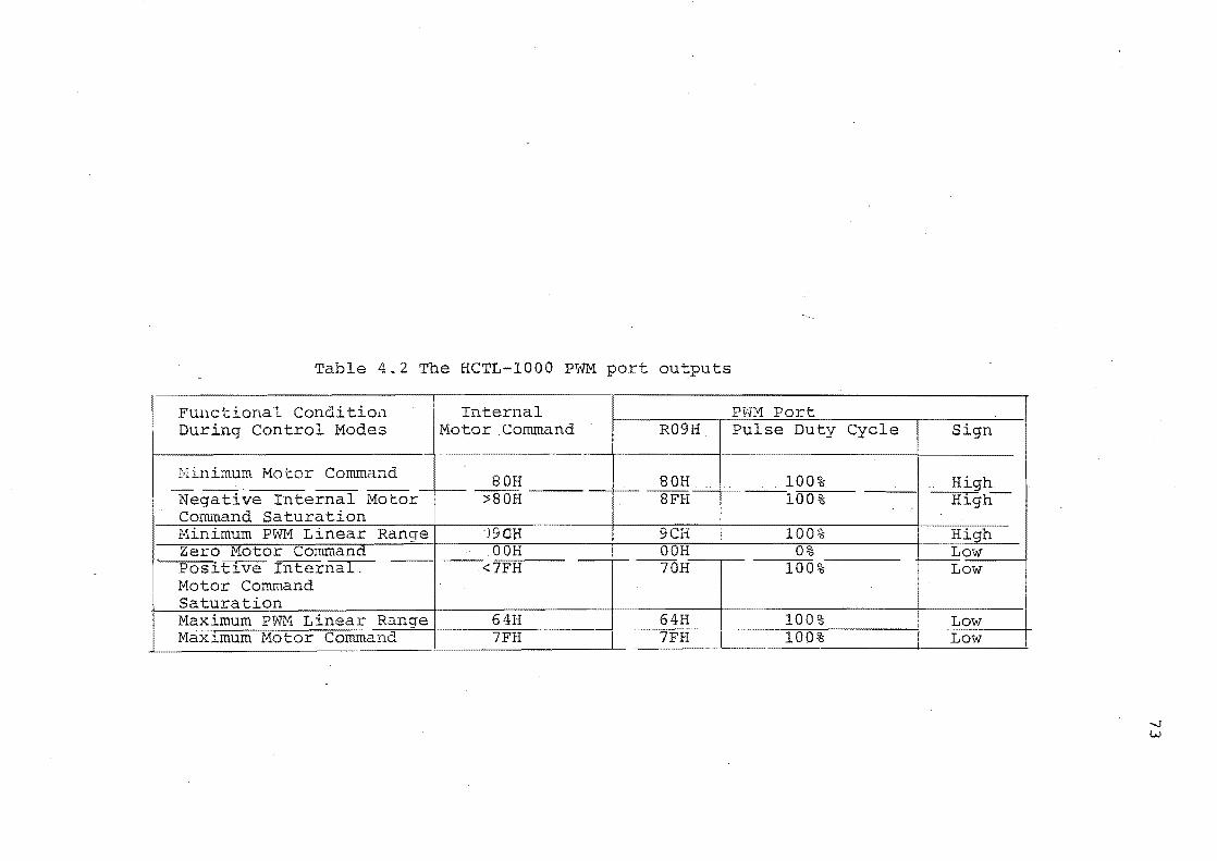
Table 4.2 The HCTL-1000 PWM port outputs
Functional Conditioa Internal P~'JM Port During Control Modes Motor.Command R09H Pulse Duty Cycle
-------
Hinimum MoJcor Commaad 80H 80H 100% -- ------Negative Internal Motor ::s80H 8PH --100% Command Saturation Hinimum PWM Linear Range ')90B 9CH 100% Zero Motor Cormnanct OOH OOH 0% ,
Positive InternaL. -- --<7FH --=roH 100% Motor Cont.TIland Saturation Maximum PWM Lin~ar Range 64H 64H 100% Maxlmum Motor Command 7FH 7FH I 100%
Sign
High ..
High-
H:i.9b. Low Low
Low Low
-
-...J W

~ g : ; 1
~
74HC"i.1.4 74HC'T1.32
Fig. 4.10 Logic circuit of the bipolar PWM motor drive
ULN2S'23
to Gate of FI
to Gate of F4
to Gate of F3
"':x:>";:t to Ga tc of F2
uso
-..J ol::>

ULN2623
c:
usc
FlU 101<
IU""
2."<2
lue; 11l1K
~13 lll:K
Fig. 4.11 Power stage of the motor· drive
cO!!
n
1~
F!25 2XZ
FlEl.A'f
+SV
.:OAV
"'::lCV
T
R27 3::lJ"!
"'12V
D
G
S
Fig. 4.12 Schematic deagram of MTP15N05E power MOS FET
'--l tn

Rl
22~R ~
R2 -4
22~R
*~ '" , ~" ..
3~
~7 II
'.
74HCTJ.4 74HCT1:32 ULN2923
'/' U50
Fig. 4.13 Logic circuit the limited unipolar PWM servo driue
to Gate F3
to Gate of FI
to Gate
to Gate F4
-...J cr.

Ion I L __ _
A B
I I --"1 ~ff. ,---
F2 ~ z:s:
Fig. 4.14 Limited Unipolar PWM motor drive current flow
77

Voltege Cv)
30
20 ,/"...-..-
Hl
20
Current. CAl
3
2.
1
"
40 60 80 t. (us)
( a)
~----~--·~'-----+-----~+-~--~I~·--~
20 40 60 80 t (lJs)
(b)
Fig. 4.15 Measured voltage and current
of the limited unipolar PWM ampl ier
78

Current (A)
3
2
1
---1-----1-1 - --......+1-----1---·_·_·· ._-+---. o 20 40 60 80 t (us]
Fig. 4.16 Motor drive transient current
waveforms
79

Velocity (radians/s) 400~---------------------------------,
300
200
100
o -100
-200
-300
bipolar
-400~---r--~--~----r---T---~--~--~
-200 -150 -100 -50 0 50 100 150 200 PWM (%)
Fig. 4.17 Motor speed vs PWM duty eye at 24V DC under limited unipolar motor drive. The PWM
80
ion range of the bipolar drive is so shown

1/
SIGN 1------------""
PULSE
Fig. 4.18 Sign Reversal Inhibit in the HCTL-1000 (by setting Status register R07H)
81
TIME

82
CHAPTER 5
SYSTEM MODELLING AND ANALYSIS
The usual requirement for a control system is that it should have good dynamic and
steady state behavior. That means the system should respond rapidly to any change in
the desired specification (e.g. position or velocity control in this application) with
negligible overshoot and a very small steady state error. To achieve this, control
theory is employed to examine the design and to predict the performance. A
mathematical model will be developed in this chapter, an analysis of the response
based on the model will be studied, and fmally. appropriate parameters will be selected.
5.1 CONTROL MODES
The versatile HCTL-lOOO executes anyone of four control modes selected by the user
through software switching for different applications, which are:
Position Control;
Proportional Velocity Control;
Trapezoidal ProfIle Control;
Integral Velocity ControL
5.1.1 Position Control
When the Position Control mode is selected, the HCTL-l 000 performs a point to point
position move with no velocity profIling. A user's program is used to specify the 24

83
bit command position for the HCTL-lOOO. The required position is compared to the
24 bit actual position, which is fedback from an encoder and measured in quadrature
counts, so that the position error is calculated. The position error is input to a digital
filter Dl (Z) which is imbedded in the HCTL-lOOO and applies full digital lead
compensation and outputs the motor drive command (c.f. Fig. 5.1). Once the motor
reaches it's destination, the controller will remain position locked until a new position
command is given.
The command and actual position data are in complemen form and reside in six 8-
bit registers. The order in which the registers are written or read is important. The
method of combining a 3-byte 2's complement word is described in APPENDIX C.
This mode provides the simplest operation among the four and hence can be
conveniently used for internal algorithm testing.
5.1.2 Proportional Velocity Control
As the name indicated, the output velocity of this mode is only proportional to the input
one. It performs control of motor speed using only the digital filter gain factor K for
compensation. The dynamic pole and zero of lead compensation are not used. The
algorithm uses the specified command velocity and the calculated actual velocity to
compute the velocity error. The velocity error is multiplied by K/4 and output as motor
command. The controller tracks the command velocity continuously. The system
behavior after a new velocity command is governed only by the system dynamics, until
a steady state velocity is reached. The units of velocity are encoder quadrature
counts/sample time. The command velocity includes a fractional part for better
resolution.

. It has been found that the data in the unlatched Actual Velocity Registers R34H and
R35H can not be read properly during movement. It is better to differentiate the actual
position to get the actual velocity.
5.1.3 Integral Velocity Control
84
Integral Velocity Control perfonns continuous velocity profiling which is specified by
a command velocity and command acceleration (c.f. Fig. 5.2). The user can change
velocity and acceleration any time to continuously profile the velocity in time. Once the
specified velocity is reached, the HCTL-lOOO will maintain that velocity until a new
command is specified. Going from present velocity to a new one, the present linear
acceleration is followed. Internally, the controller perfonns velocity profiling through
position control, therefore the complete dynamic compensation Dl (Z) is used. From
the user specified command velocity and acceleration, the controlle internally generates
the required position profiles. In control theory tenns, integral compensation has been
added and therefore, this system has zero steady state velocity error. However, the
detrimental aspect of this compensation is that, the loop stability compensation is more
difficult to achieve.
This mode is used in the project so that the antenna can track satellites according to the
required velocity and acceleration profile. Unexpected position changes are followed
and the sophisticated coordination of six motors' movement is kept.
5.1.4 Trapezoidal Profile Control
Trapezoidal Profile Control perfonns point to point position moves and profiles the
velocity trajectory to a trapezoid or triangle. The motion is determined by the specified
acceleration, maximum velocity and final position. The HCTL-lOOO computes the
necessary profile to confonn to the command data. If the maximum velocity is reached

85
before the distance halfway point, the profile will be trapezoidal, otherwise the profile
will be triangular. Possible trajectories with this mode is shown in Fig. When
the move is finished, the position control locks on the final position. The controller
actually performs position control while the profile generator continuously updates
profile data into the Command Position registers. Full digital compensation is applied
by the digital filter.
During the above four control modes, the HCTL-lOOO also provides commutator
controL The user can properly select the phase sequence for electronic commutation of
multiphase motors like step or brushless DC motors.
A program was written to run the motor under each control modes. The flowchart is
shown in Fig. S.4.and the program is attached in APPENDIX C.
As indicated in last chapter, the motor drive adopted is a PWM drive in which the
current is variable while the voltage is a constant. This voltage relations of permanent
magnet DC motor, derived from Eqs. (4.3) and (4.5), can be expressed as
(5.1)
Here the impressed voltage is treated as the function of time t explicitly. At any time
instant, the mechanically developed torque must be equal and opposite to the sum of
the torques necessary to overcome the friction, inertia, and load torque. When the
friction (viscous and Coulomb) torque is neglected, this developed torque is:

86
(5.2)
Where, J - total moment of inertia of the rotor and the load referred to the motor
shaft;
de 1 l' - angu ar acce eraUon.
This torque must be equal to the electrically developed torque as shown in Eq. (4.4),
so,
(5.3)
Thus, the combination of Eqs. (5.1), (4.4) and (5.2) gives the relationships of voltage
and angular velocity:
Taking Laplace transform of both sides of (5.4) leads to
So, the transfer function of the motor becomes
n (s) K t Om (s) == V (s) ::= R J s + K K
mat e 1 + 1: S
(5.4)
(5.5)
(5.6)
Where, Km::= 1 :::: 0.673 ::::: 13.7 (radian/volt.s), Km is called the motor constant;
R J "C:::: K a
K ' is called the motor time constant. By experimental measurement,
t e
the time constant 1: 0.114s.

87
Substitute these value into (S.6), the motor transfer function is
G () 13.7 m S =0.114s+1
Then the angular position is:
Km Yes) 13.7 yes) 8(s)=---= 2
s(I+'ts) 0.114s +s (S.7)
S.2.2 The Encoder
The feedback in the system is achieved by an incremental encoder. The principle of the
encoder is schematically shown in Fig. S.S(a). The rotating disk which has SO radial
slots is mounted on the shaft of the motor. There are two OPB960 Slotted Optical
Switches fixed on the motor bracket, apart from each other by almost 180·. The
rotating disk is inserted through the slot of each optical switch. Each switch has a light
source and a light sensor. Once the sensor receives light, the output will be a high
voltage" 1", else the output will be a low voltage "0". When the disk rotates, its teeth
block the light passageway discretely and two trains of rectangular pulses will be
output from the switches.
The phasing of the two output pulse trains, one is called channel A (CHA) and the
other is called channel B (CHB), is adjusted to be 90· apart, i.e. in quadrature, as
shown in Fig. S.S(b). These signals from CHA and CHB are output to the quadrature
decoder/counter in the HCTL-I000, (each interval is counted 4 times to give 200
counts per revolution) as feedback signals of the motor shaft position. The quadrature
decoder/counter can detect the direction of the rotation by decoding the relative angles
of CHA and CHB, and count the number of pulses in 2's complement word form.

88
The number then is sent to the Actual Position registers R12H, R13H and R14H to
give the shaft mechanical position information. When combined with the lead screw
pitch of 0.2", the resolution is 0.001" per count.
5.2.3 The Control System Modelling
An overall system diagram of the computer, the HCTL-lOOO and the motor drive is
shown in Fig. 5.6(a). The input, output and transfer functions of each part are
indicated.
R(Z) is the Z-transform of the digital input from the host processor IBM-PC. Dl (Z) is
the programmable digital filter imbedded in motor controller chip HCTL-lOOO. The
digital filter is used to compensate for closed loop system stability. The compensation
is a first order lead filter in combination with the sample timer T, which is stored in
register ROFH of HCTL-lOOO and effects the dynamic step response and stability of
the control system. It has the form
K (Z - A / 256 ) ( Z - a ) Dl (Z) = Z + B /256 = Kg Z+ b
Where, Z - digital domain operator;
Kg = K/4, K is the "gain" number in R22H;
a = N256, a is the zero of the filter;
b = B/256, b is the pole of the filter;
A and B are manufacturer defined "zero number" and "pole
number" residing in the R20H and R21H registers.
(5.8)

Note that the maximum output of the digital filter has been limited to 100 by saturated
PWM pulses (giving 100% duty cycle) (c.f. Fig. 4.18). The error e(k) between the
system input and output is
e(k) = r(k) - y(k) (5.9)
This error (Z form) then is input into the digital filter Dl (Z) to become G(Z). So the
transfer function is
O(Z) (Z - a) Dl (Z) = E(Z) = Kg Z + b
The output sequence g(k) from the filter is described as
g(k+ 1) Kg e(k+ 1) - a Kg e(k) - b g(k) (5.10)
89
Eq. (5.10) becomes an evaluating equation for the digital filter performance. So the
final output of the digital filter is
{
g(k) f(k) =
100
g(k) < 100;
g(k) >= 100 (5.11)
The PWM output is equivalent to a digital to analog output This is represented in Fig.
by the impulse train generator and zero-order hold which are imbedded in HCTL-
1000 unit to convert digital signals to analog signals. The zero-order hold has the form
1 - sT - e s

Where, T is the sample time. Then, for the part within dotted line in Fig. 5.6 (a),
analog transmittance D2(s) is
-sT (1 t =K (l-e ) ---+ m 2 S S
hence the corresponding Z-transmittance is
1 [ TZ D2(Z) :: Km (1 - Z· ) 2 (Z - 1)
tZ tZ +--
-T/ Z - e
==K (nZ-p) K (Z-h) m (Z - 1) (Z - c) 1
-T/'t Where, C:: e
n == T + 1: (c - 1);
P = T c + t (c - 1);
h:::: pIn.
The transfer function
Kl (Z - h) Y(Z) D 2(Z) = (Z-l) (Z-c) :: F(Z)
(5.12)
(5.13)
90
So this discrete time system overall output sequence is described by a difference
equation:

y(k+2) == Kl f(k+l) ~ h Kl f(k) + (1+c) y(k+1) - c y(k) (5.14)
Note that the third order model in Fig. 5.6(a) reduces to the second order model shown
in Fig. 5.6(b) when PWM :::: 100%. The analysis of this model for a large step input
(c,f. Fig. 5.6(b» is given in APPENDIX A.
5.2.4 Theoretical Response
A series of initial conditions may be defined for Eqs. (5.9), (5.10), (5.11) and (5.14).
Assume the input ret) is a step input with amplitude of Ap and the output of the system
8(t) cannot respond to ~e input until the initial two sample time periods after. The
initial conditions are
r(O):::: Ap
r(l):::: Ap
y(O):::: 0
y(1) == 0
e(O) :::: reO) - yeO) == Ap
e(1) :::: r(1) - y(1)::: Ap
g(O) == Kg e(O) == Kg Ap
91
Then the theoretical response of the system can be obtained. A computer program was
written to calculate the step response (c.f. APPENDIX C). One example of the system
theoretical response under position control mode is shown in Fig. 5.8(a). It can be
seen that in the beginning, the response is nearly linear and represents constant speed.
This reflects the effect of the 100 (%) limit in the PWM signal when the error is big.
This constant applied voltage is opposed by the back emf produced at constant speed.
When the response approaches the specified position (~:::: 1000 quadrature counts),

the applied voltage is reduced (PWM < 100%) and the response is detennined by the
values of the parameters residing in the filter.
92
With the same parameters chosen, an experimental response of the motor was
measured and plotted shown in Fig. 5.7. Comparison of the two diagrams shows that
the theoretical model has a good agreement with the experimental one. Because the·
motor shaft friction and the armature inductance were neglected when simplifying the
motor model, the slight difference in the slopes is expected, i.e., the motor's maximum
speed is less than predicted when friction is neglected. The slight differences shown in
the overshoot damping rate is most likely caused by Coulomb friction in the motor.
This reduces the overshoot amplitudes and gives a faster damping rate. Hence, this
theoretical model can be used for choosing parameters in the filter.
A detailed discussion about the effect of the friction is given in APPENDIX B. Fig.
5.8(b) is the theoretical response based on the model in APPENDIX B. Agreement
with the experimental response is excellent.
5.3 EXPERIMENTAL RESPONSE ANALYSIS
Several groups of response data were collected by varying the parameters T, A, B and
K in the prograrnmable digital filter Dl (Z). These were plotted in Fig. 5.9, 5.10 and
11.
If a closed loop system can not obtain adequate performance by using Gain K and
output feedback alone, additional transmittances or compensation may be added to the
system. These will improve the relative stability, steady state error or the step response
overshoot.

93
It can be observed from Eq. (5.10) that the Gain K is most effective and depends on
the last input sequence, i.e. the first to react to the input. The A has a moderate effect
to compensate the K. The B plays a small part, and its effect depends on output status
only. These effects can also be seen from the graphs. Sample time T has been fixed at
111111s or ROFH 127. Fig. 5.9 shows a group of response solely under the effect
of K. When K varies from 1 to 74, it markedly changes the response from having an
overdamped response with a big error to being lightly damped. In addition, the error
in approaching the specified position cannot be removed only by adjusting K and not A
and B as compensators. The group shown in Fig. 5.10 illustrates that the A gives an
effective range of compensation to improve the stability and error when varied from
150 to 252. Although B has least effect as shown in Fig 5.11, when varied from 40 to
255, it improves the rise time slightly. It can be used as a fine compensation factor.
5.4 SlJMMARY
The HCTL-lOOO unit gives multiple choice in control modes which can be
conveniently used in various applications to meet each particular requirement
Except for Proportional Velocity Control mode, the algorithm of which is only
governed by the Gain factor K, the other control modes all execute specified profile
with lead compensation. This gives flexibility to achieve the desired motor
performance.
The mathematical model of the whole system can be used as a tool for choosing the
filter parameters. When the error between the input and output is small, the behavior
of the system is dominated by the digital filter; and when big, by lOO*D2(Z) due to the
saturated PWM port output

COMMAND VELOCITY
R241-1 MSS AU'" LSB t' ......
'" '" ..... COMMAND POSITION
ROCH MSB I--'
//
//
ROOM ROEM lS8
-1 I I I I
POSITION PROFilE CENERAT10N
UNTEGRAL TRAPEZOIDAL VELOCITY PROFILE
R27H ACCEI. MSS AITM ACCEL MSS R2SH ACCEl l SS R26H ACCeL LSS RXH COMMAND R2SH MAXII'o4UM
VELOCITY VELOCITY lUSH FINAL POS. I'o4SS R2AI-I "INA!. pas. R29'H FINAL POS. lSS
I!I BIT PARALLEL MOTOR COMMAND PORT
ROSH
R20H JI\ AltH a R21t-f 1(
SAMI"lE TIMER
FlOFH
PWM MOTOR COMI'o4ANO PORT
R09I-f
\: ________ J ,,"'" .....
COMMUTJI,TOR
/ ......... r--------&<-/----, r----.... - .... ~-------,
I ACTUAL VELOCITY L I ::,~~~OSITlON I RJSH MSI!I -i'\JAH LSS
eHA CHili
CON FIGURA nON REGISTERS
!'118M RING RtAH )( A1BM Y RICH OFFSET RtFH MAX ADVANCE R19M VELOCITY
TIMER·
flOCH FLAG REGISTER ROSH PROGRAM COUNTER Rom STAruS REGI~eR
Fig. 5.1 Register Block Diagram of HCTL-IOOO
MCo- I'o4Cl
PULSE SIGN
""'A-I'1-I0
1..0
"'"

VELOCITY
CVEL "COMMAND VELOCITY RJCH A::: ACCELERATION R26H. R27H
(0 USER CHANGES ACCELERATION COMMAND
o USER CHANGES VELOCITY COMMAND
Fig. 5.2 The HCTL-IOOO Control Mode
Velocity
."...--------.,.--- MAXIMUM VELOCITY
VELOCITY FO SET BY USER
TRAPEZOIDAL
-t---- MAXIMUM VELOCITY
VELOCITY
TRIANGULAR
FO CLEARED BY HCTL-1000
FO CLEARED BY HCTl-1000
FINAL POSITION
Fig. 5.3 The HCTL-IOOO Trapezoidal Profile Control Mode
95

set Position Control flag FO=O, F3=O,
F5=O
enter Command
Position
start
Fig.5.4 Flowchart for six motor four mode control
choose control mode
choose fIlter parameters
set Proportional set Integral Velocity flag Velocity flag
F3=1 F5=1
enter Command enter Command
Velocity Velocity and Acceleration
moniLor running Actual Velocity .
go to Starting Position
enter .Maxirmun Velocity &
Acceleration
set Trapezoidal ProfIle flag FO=l
96

'.
F . 5.5 Principle and output signals of the duel-channel encoder
A LIGHT [M!TTING mODE /
INTERUPT!:R DISI(
LIGHT PATH B DPTO DEVICE
'WaveforM frOM 5v r----,
Opto Device A
usedns reference
during rotation
VoveforM fron B showIng phasE' dlff
erence when rotating
Ov
5V
In 0. given direction Ov
'WaveforM frOM B 5v
shOWing phase shiFt
when rotating in the
opposite direction Ov
1 I
-
-
I
I
r-I
I~
!
,E
:-
I 1 1 I '--
,----
I
97
'.

. ..;. ......
ret) r(k) + _ e(k) --I"'I11\10~ AID I ~ R(s) i I R(Z) _T E(Z)
y(k)
Fig. 5.6(a)
D2(Z)
j---------------------------------------, i i
I e~
f* l-e -sT Km 1
s
~--------------~vr----------------J
i ~(S) I i _______________________________________ _
Computer, HCTL-IOOO and DC motor control
yet)
yes)
e
1..0 co

ret) .. Limit
R(s)
100 Km m (t) 1 ~ ~ .. -..
1 +1: S !l(s)
Fig. 5.6(b) System diagram under large step inputs
s
99
e (t) yet)
,.. yes) 8(5)

Quadrature counts
1000
sample time = 111 Ips A=O B=O K=30
200 samples
Fig. 5.7 Experimental response in position control
mode (motor No.2)
t
Quadrature counts
1000
o
sample time=llllps A=O B=O K::::::30
200 samples
Fig. 5.8(a) Theoretical response in position control
mode assuming negligible friction
100

1000
o
counts
Fig. 5.8 (a)
sample time=llllMS A:::; 0 B=O K=30
200 samples
response in position control
mode assuming negligible friction

1000
ture
sample time = lll~s A = 0 B = 0 K == 30
200'samples
Fig. 5.8(b) theoretical response in position
control mode including friction allowed for by
a 20% reduction in the available supply voltage
101

Quadrature counts
2000
(()
.w s:: ;::l o o o o N
a
T=llilus A=O B=O
142ms
.~-------------l--------------+--'-----.-- ---------1-. __ .. -.------- ---+----- ---- -----.~
t
Fig. 5.9 The effect of the digital filter Gain K (from the enlarged end region of the position time profile measurement under position Control)
f-! o N

Quadrature counts
2000
til .jJ f.:! :::1 o ()
a a
A=lS0
/
T=llllus B=O K=127
l42ms
N ..J l----------------------J ---------------4-------- --- ---------+----- --- +-------- -- ---I o t
Fig. 5.10 The effect of the digital filter Zero A (from the enlarged end region of the position time profile measurement under Position Control)
I-' a w

Quadrature counts
Ul +l ~ ;:1 o o o o N
J o
T=llll.us A=127 K=127
142ms
t
Fig. 5.11 The effect of the digital filter Pole B (from the enlarged end region of the position time profi measurement under position Control)
I-' o ,I::>

105
CHAPTER 6
CONCLUSION
This study has embraced the analysis, design and development of multi-axis machinery
numerical controL
The mechanical problems in existing satellite tracking systems and heavy duty robots
and the like have been addressed by means of a multi-axis machine with six degrees of
freedom i.e., a Stewart platform parallel robot mechanism.
Driving multi-axis machinery with conventional direct numerical control and a single
computer software control has considerable limitations. When the speed change of the
motor is high, insufficient torque will cause motor speed drop and it may stalL Hence
a new type of IC controller, the HCTL-lOOO has been combined with the computer to
drive motors.
An IBM PC controller board based on above IC was designed to control six motors
which drive the six linear actuators required for the Stewart platform. The controller
has proved capable of fulfilling the fast positioning and high precision control tasks.
The DC motors can be driven under Position, Proportional Velocity, Integral Velocity
and Trapezoidal Profile Control modes.
In addition, a motor drive PWM servo amplifier was designed. Both bipolar and
limited unipolar PWM drives were examined. The bipolar type was not suitable for
this application, as it could not drive the motors when the PWM duty cycle was below

106
60%. The linear operating range of the motor speed control was too small. Thus a
limited unipolar PWM drive stage was used. This provided sufficient current to the
motor and gave a high efficiency drive system with a dead zone of less than 10%
(when the rubber seals on the lead screw was well lubricated).
A mathematical model of the whole system has been developed and gave good results.
When friction effects were incorporated, the theoretical model results and the
experimental results are in excellent agreement. Thus the theoretical model proved
useful for designing the system and predicting the system performance.
More applications can be developed from the results of this research. Drives for DC
brushless and step motors, and for hydraulic cylinders can be based on the same motor
controller board. These are topics for further research and development.

107
APPENDIX A
SYSTEM PERFORMANCE FOR LARGE STEP INPUTS
It is pointed out in 5.2.3 that, fora large step input to the system, the system
perfom1ance is determined by a fixed output of PWM port and reduces to a second-
order response (c.f. Eq. (5.14) and Fig. 5.7).
Assume a step input to the system is 22 volts, which is the 24V power supply less a 2 volts drop across two field effect transistors. The input is ret) 22 u(t) or
R(s) = s
so the output of the system is
Y(S)=( ~)(~)(~)=22~(~~2..+ 't J 1 + t s s s s2 s 1 -+s 't
Taking the inverse Laplace transfom1, the position output is
-t/'t -t/'t yet) = 22 Km (t - t + 1: e ) u(t) = 22 ~ (t + 't Ce 1» uCt)
Therefore, the output velocity is
1 t/7; -t/'r ro(t) = 22 Km [ 1 + 1: (- - e )] = 22 Km (1 e )
't

108
The second term shows the transient response after t = O. With t increasing, the
velocity tends to be constant This is observed at the beginning of the movement
shown on the plotted graphs in Fig. 5.8 and the measured response in Fig. 5.7.
The theoretical response when PWM = 100% is plotted below and shows good
agreement with the actual measured response.
y( t)
o
T
I
~ slope=22K m
t

109
APPENDIX B
ANALYSIS OF FRICTION EFFECTS
The effect of the friction is discussed here and a more accurate mathematical model is
obtained by incorporating some simple corrections.
Current Consideration
When the model of the motor was made, the viscous and Coulomb frictions were
neglected (c.f. Eqs. (5.2) to (5.6». If the effect of the friction is considered, the extra
torque TfT caused by the friction must be also overcome by the developed torque Tm,
and Eq. (5.3) becomes
(B-1)
From the manufacturer's graph shown in Fig. 4.6(a), the no load current is 3 Amps at
maximum speed. Thus at least 3 Amps are required to overcome the friction drag. dO)
When dt = 0 (no extemalload and at full steady speed), then
So in both with load or without load conditions, Eq. (5.3) becomes

110
or (B-2)
Note that in Eq. (B-2), Ia has an extra tenn "-3" which is not included in Eq. (5.3).
Also note that the viscous friction force is a retarding force which is proportional to
velocity. Coulomb friction is also a retarding force of constant magnitude with the
sign of the frictional force changing with the reversal of the direction of velocity. In
general, the friction always opposes the motor motion, so that when
OJ > 0, (I. - 3) (I I. 1 - 3) (I :: 1 J , the effective current is less hence the acceleration is reduced. In addition, the
maximum speed is less than without friction. When ro >0, and la < 0, the condition
occurs on position overshoot, the effective current is larger by 3 Amps. This causes
the position e (t) to settle to the specified position more quickly. In other words, the
friction (mainly Coulomb friction) helps to reduce the overshoot or undershoot of the
motor output. This friction effect can be observed from the experimental response
graph in Fig. 5.7. The overshoot and undershoot region shows smaller overshoot
amplitude and faster setting. Finally, the Eq. (5.4) becomes
or,
Voltage Consideration
The PET saturation will decrease the effective voltage by about 2 volts. The way to get
around this is to recognise that the PWM signal only operates with the full voltage
available. When the motor perfonns under the conditions of 24V power supply, 2

111
volts saturation voltage drop and the motor armature drop, the effective voltage
Vefis
Vef = ex 24 (volts) = 24 - 2 - 3 Ra == 24 - 2 - 3 * 0.9 = 19.3 (volts)
So, ex == 19.3/24 == 0.80
where ex is the effective voltage coefficient. Then the Laplace transform of the motor
input is
V m'(s) = Vef (PWM%) == 24 ex (PWM%) == ex V m(s)
where V m(s) is the original input in CHAPTER 5. So Eq. (5.6) is modified to
or
G'm (s) = O(s) aV m(s)
K K' ex m m Gm'(s) :::: a Gm = --- = --
l+'&s 1+'&s (B-3)
where Gm' and~' are modified values when consider the effective voltage. ~'
reduces the gain Kl in Eq. 5.13 by a, and thus reduces the slope of the step response.
Corrections
It has been pointed in CHAPTER 4 that the motor could be driven at 10% PWM duty
cycle. Three months later when obtaining the data needed in Figs. 5.7 and 5.8, it was
found that 20% PWM was needed to obtain a slow speed. Thus at least 20% of the
available voltage is used simply to overcome the increased friction caused by the oiled

112
seals drying out. Therefore a = 0.8 is calculated from both the voltage drop and the
PWM output (Le., 100% - 20% := 0.8).
Examine the slopes (i.e. the speeds) from Figs. 5.7 and 5.8(a), the experimental slope
is
Kex = 61.2 (radians/s)
The theoretical slope (no friction allowances) is
Kth = 74.6 (radians/s)
When consider the effect of (x,
Kth = 74.6 (X := 59.7 (radians/s)
This shows a very good agreement with the experimental result. So a should be
applied in the mathematical model when more accurate results are needed. When this
is done, the response shown in Fig. 5.8(a) is modified to that shown in Fig. 5.8(b).
The theoretical response is now very close to the measured response in 5.7.
Friction Problem
The problem noticed here is the increased friction in the motor. The extension tube
support contains the rubber O-ring seals which dry out. When they are lubricated, the
friction decreases. To avoid this friction problem, the seals should be replaced by
grease impregnated felt seals to give smaller and more constant friction.

113
APPENDIX C
10 REM PROGRAM 1 : RNW 20 REM Reading or writion a register. The command form is RRXXDDC. 30 'RR is a LSB of a register except for ROCH (MSB for it), with 40 'an "h" end if a hex number entered. XX represents Read or 50 'Write. If a 3-byte datum to be read, enter "1'1'1"'; if a 2-byte GO 'datum to be written, enter "ww", and so on. DD is a datum to 70 'be written to the register, with an "h" end if a hex. C is 80 'optional if reading continuously. 90 REM Press BREAK key for pause any time and press F5 for resuming. 100 REM 110 REM Configuration **1' •• **.*****.** •• ************************ 120 REM Processing input string, seperating it into three parts. 130 PRINT 140 INPUT"Enter command (all LSB but MSB for ROCH)"; X$ 150 PRINT 100 A$= .... : B$="": C$='''' 170 IF X$="" THEN 140 180 FOR P=l TO LEN(XS) 190 Q$=MIDS(X$,P,l) 200 IF Q$="R" OR Q$;;;:"r" THEN B$=B$+"R": GOSUB 310 210 IF QS="W" OR Q$="w" THEN B$=B$+"W": GOSUB 310 220 NEXT P 230 T$=A$: GOSUB 350: R%=N# 240 T$=C$: GOSUB 350: D#=N# 250 BYTE=LEN(B$) 2GO BBS=LEFT$(B$,l) 270 IF BB$="R" THEN GOSUB 410 280 IF BB$="W" THEN GOSUB 750 290 IF TT$="C" OR TT$;;;:"c" THEN 270 300 GOTO 140 310 REM seperating AS and C$ from XI. 1*'***1*1111**1*'*'****1* 320 IF AS:'''' THEN A$=LEFT$(X$,P-1) 330 C$=RIGHT$(X$,(LEN(X$)-P)) 340 RETURN 350 REM Converting A$ and C$ to numbers. **1***1**1'*********** 3GO TT$=RIGHT$(T$,l) 370 IF TT$="H" OR TT$ "h" THEN T$="&H"+T$ 380 N#=VAL(T$) 390 RETURN 400 REM 410 REM Reading *****1*1***1******'*'**********'**********'*** 420 RR%=R% 430 FOR S=l TO BYTE 440 GOSUB G80 450 IF S 1 THEN K%=D%: K$=HEX$(D%): PRINT" LSB";D%,"or Hex H;K$ 4GO IF S=2 THEN J%=D%: J$=HEX$(D%): PRINT" MB ";D%,"or Hex "jJ$ 470 IF S=3 THEN I%=D%: I$=HEX$(D%): PRINT" MSB";D%,"or Hex ";1$ 480 IF R%=20 OR R%=19 OR R% 18 THEN RR%=RR%-l ELSE RR%=RR%+l 490 NEXT S

500 ON BYTE GOSUB 520, 580, G30 510 RETURN
114
520 REM Converting a I-byte number to negitive one if it is. * 530 8UM#=K% 540 IF K%>127 THEN SUM#=SUM#-256# 550 8UM$=HEX$(8UM#) 560 PRINT" The sum is u;8UM#,"or Hex ";8UM$ 570 RETURN 580 REM Combining a 2-byte number and/or oonverting to negitive 590 8UM,=J%*256#+K% 600 IF J%)127 THBN SUM#=8UM#-65536# 610 PRINT" The sum is ";8UM# 620 RETURN G30 REM Combining a 3-byte number and/or converting to negitive 640 8UM#=(I%*25G+J%)*256+K%: G50 IF 1%>127 THEN 8UM'=8UM'-1677721G# 6GO PRINT" The sum is ";8UM#: PRINT G70 RETURN G80 REM Reading a byte from a register. *********11*"******** 690 OUT &H308,RR% 700 DIX=INP(&H300) 710 D%=INP(&H308) 720 PRINT" Read in from register ";RR% 730 RETURN 740 REM 750 REM Writing **,**t*,,***********,************************* 7GO FOR 8=1 TO BYTE 770 ON BYTE G08UB 850,890,940 780 IF 8=1 THEN D%=R% 790 IF 8=2 THEN D%=J% 800 IF 8-3 THEN D%=I% 810 GOSUB 1000 820 IF R%=20 OR R%=19 OR R%=18 THEN R%=R%-1 EL8E R%=R%+1 830 NEXT S 840 RETURN 850 REM Converting to 2's com of a I-byte number. ************ 860 IF D#<O THEN D#=D#+25G 870 K%=D# 880 RETURN 890 REM Converting to 2's com, seperating into 2 bytes. ****** 900 IF D#<O THEN D#=D#+G553G# 910 J%=FIX(D#/25G) 920 K%=D#-J%*25G 930 RETURN 940 REM Converting to 2's com and seperating into 3 bytes. *** 950 IF D#<O THEN D#=D#+1677721G# 960 I%=FIX(D#/G5536#) 970 J%=FIX(D#-I%*G553G#)/25G) 980 K%=D#-I%*65536#-J%*25G# 990 RETURN 1000 REM Writing 1 byte to a register. ************************ 1010 OUT &H308,R% 1020 OUT &H300,D% 1030 PRINT" Output the datum"jD%;"to the register";R% 1040 RETURN

REM PROGRAM2: PERFORM6 REM This is a general testing program for performing every REM control mode of HCTL-lOOO controller and driving six REM motors.
115
t"""",.t"""""",ttt"""""",."""",t"","" CHOOSE MOTORS
"""""""""""","",.""""""".,.",,,,,""",
Portl=&H300 Port2=&H308
Motor: CLS
'set I/O addresse
INPUT "Run which motor (Enter motor number 1, 2 .•. )" M% Portl=Portl+M%-1 Port2=Port2+M%-1
,," t'""", t t, t' t, t"" l' t"""" t, t" t t, t" ,,t t t t'" t t'" t
CONFIGURATION
"""""""""""""""""""""""""""11"1'
R%=&H5: D%=O: GOSUB WriteOut R%=&H7; D%=l: GOSUB WriteOut
Idle: R%=&H5: D%=l: GOSUB WriteOut
Isoftware reset 'PWM Sign Reversal I Inhabit
'Initialization Idle
111111111111I111I1I1I1I111111111111111I111111111111111111111
CHOOSE CONTROL MODE AND FILTER PARAMETERS
1""""""""""'1"'1'11'1""1,1",1""'11',,,""1'
Order:
CLS
'mode and filter I command
PRINT"Enter oommand ss,zz,pp,gg,mm" PRINT PRINT" PRINT" PRINT" PRINT PRINT" PRINT PRINT" PRINT PRINT" PRINT PRINT" PRINT" PRINT" PRINT" PRINT" PRINT
ss:
zz:
pp:
gg:
mm:
Sample Time" B.G80G-2222.233Gus for OP and PV modes" G9.4448-2222.233Gus for IV and TP modes"
Zero A, 0<-A<-255"
Pole B, 0<=B<=255"
Gain K, 0<=K<=255"
oontrol mode" PO for Position Control" PV for Proportional Velocity Control" IV for Integral Velocity Control" TP for Trapezoidal Profile Control"
'get command string and seperate it

LINE INPUT OrderS PRINT Pie%:I: PieBg%=l FOR Comma%=1 TO LEN (OrderS) Cma$=MID$ (Order$, Comma%, 1)
116
IF Cma$-II," THEN Pie$=MID$ (Order$, PieBg%, Comma%-Piebg%): PieBg%=Comma%+I: ON Pie% GOSUB SReg, ZReg, PReg, GReg: Pie%::Pie%+1
NEXT Comma% Mode$=RIGHT$(OrderS,2)
SELECT CASE Mode$ CASE II PO" , "po"
GOTO PosiCtr CASE "PV", "pv"
GOTO ProporCtr CASE "IV", "iv"
GOTO InteCtr CASE "TP", "tp"
GO TO TrapeCtr CASE ELSE
GOTO Order END SELECT
t,t""""""""""""""", •• "".",."""",""t" POSITION CONTROL
". ""1,,11""""'1' ,,1""" 1""1"1"'1'1'1 """ .,.,' I
PosiCtr: 'set flag register
R%=&HO: D%=O: GOSUB WriteOut D%=3: GOSUB WriteOut D%=5: GOSUB WriteOut
'tell aotual position GOSUB AoPosi AoPosi# = Sum# CLS PRINT PRINT"The Aotual Position is "; AoPosi#
INPUT"Enter Command Position -8388G08<=P<::8388G08";CmPosi# 'seperate input number into three bytes
TriBy# = CmPosi# GOSUB TriSepe
'send into Command Position registers R%=&HC: D%=I%: GOSUB WriteOut R%=&HD: D%=J%: GOSUB WriteOut R%-&HE: D%=K%: GOSUB WriteOut
'ready? go! R%=&H5: D%::&H3: GOSUB WriteOut
MoniPosi: GOSUB Emerg

'monitor excution to see if it's completed GOSVB AcPosi: print sum#
117
IF CmPosi# > AcPosi# THEN IF(CmPosi#-Sum#)O GOTO MoniPosi ELSE GOTO Comple
IF (CmPosi#-Sum#)<=O THEN GOTO MoniPoei ELSE GOTO Comple
Comple: PRINT PRINT"Motion completed."
R%=&h9: D%=O: GOSUB WriteOut
PRINT"Enter new position? (YIN)" GOSUB WKey IF AKey$="Y" OR AKey$="y" THEN GOTO PosiCtr
PRINT"Run another motor? (YIN)" GOSUB WKey IF AKey$="Y" OR AKey$="y" THEN GO TO Motor
GOTO Idle
1.,.1.1,1.1111111111111111111111111111111111111111111111',"
PROPORTIONAL VELOCITY CONTROL
ttl.t.,.tttt ••••••• ,.""., •• """"" •• """"".""",t
ProporCtr: 'set flag register
R%=&HO: D%=ll: GOSUB WriteOut
Restart: CLS INPUT"Enter Command Velocity _2047.o000(v<2047.0000";CmVel#
'deal with Command Velocity for R24H and R23H CV#=CmVel#*lG IF CV#<O THEN CV#=CV#+G553G# J%=FIX(CV#/25G#) K%=FIX(CV#-J%*Z5G#)
R%=&H24: D%=J%: GOSUB WriteOut R%=&H23: D%=K%: GOSUB WriteOut
'ready? go! R%=&H5: D% &H3: GOSUB WriteOut
AcVel: Iread in and print Actual Velocity
R%=&H35: GOSUB ReadIn: J%-D% R%=&H34: GOSUB ReadIn: K%=D% GOSUB TwoCornbine PRINT" The Actual Velocity is" TAB(2G) TwoSum# PRINT TAB(45) "The command Velocity is"; CmVel#
LOCATE 25,1 PRINT"Press V to give a new Command Velooity,"; PRINT" other keys to exi t"

GOSUB Emerg
WHILE NOT INSTAT GOTO AcVel WEND
AKey$ ;:: INKEY$ IF AKeY$="V" OR AKey$="v" THEN Restart
R%=&H24: D%=O: GOSUB WriteOut R%=&H23: D%=O: GOSUB WriteOut
PRINT"Run another motor (YIN)" GOSUB WKey
'stop motor
IF AKey$="Y" OR AKeY$-"y" THEN GOTO Motor
GOTO Idle
118
""'1""""""""""""""""""""""""I"", INTEGRAL VELOCITY CONTROL
1""'11""""""""""""""""""""""1'"""
InteCtr: Iset flag register
R%=&HO: D%=13: GOSUB WriteOut
CLS PRINT INPUT"Enter Command Velocity -127<=V<=127"j CmVe12% GOSUB CmVe12 INPUT"Enter Acceleration O.OOOOOOOO<A<:::127.00000000"; Acce# GOSUB Accele
LOCATE 23,1 PRINT"Enter Vnumber to give a new Velocity" PRINT", Allumber to give a new Acceleration," PRINT" others to exit."
R%=&H5: D%=3: GOSUB WriteOut
NewCom: GOSUB Emerg
WHILE NOT INSTAT: WEND LINE INPUT X$
VorA$ ::: LEFT$ (X$,l)
Num$ ;:: RIGHT$ (X$, (LEN(X$) 1))
IF VorA$="V" OR VorA$-"v" THEN CmVe12%=VAL(NumS): GOSUB CmVe12: GOTO NewCom
IF VorA$="A" OR VorA$:;lI a " THEN Acce#=VAL(Num$): GOSUB Accele: GOTO NewCom
CmVe12%=O: GOSUB CmVe12 Istop motor
PRINT"Run another motor (YIN)"

119
GOSUB WKey IF AKey$ "Y" OR AKey$="y" THEN GO TO Motor
GOTO Idle
, , t , , , , , t , , , t , , , , , , , , , , , , t t t t , , , , t , , , , , , , , t t t t , , , , t t t t , , t t t t
TRAPEZOIDAL PROFILE CONTROL
t , , t , , t t , , t , tIt t , t , t , , J , , t t , t , , , , t , , , t , , , , , , , , , , , t , , , I , t t , , ,
TrapeCtr: ttell Actual Position
CLS GOSUB AcPosi PRINT PRINT"The Starting Position is"; Sum; PRINT"Are you satisfied? (YIN)" GOSUB WKey IF AKey$="Y" OR AKey$="y" THEN Start;=Sum#: GOTO FinalPosi
'utilize Position control mode R%=&HO: D%=O: GOSUB WriteOut
D%=3: GOSUB WriteOut D%=5: GOSUB WriteOut
PRINT"So what's your Starting Poisition"; INPUT" (-8388G08<=Start<8388G08)"; Start#
'adjust Starting Position TriBy# = Start# GOSUB TriSepe
R%=&HC: D%=I%: GOSUB WriteOut R%=&HD: D%=J%: GOSUB WriteOut R%=&HE; D%=K%: GOSUB WriteOut
'ready? go! R%=&h5: D%=3: GOSUB WriteOut
GOSUB Emerg
FinalPosi: INPUT"Enter final Position -8388G08<=Final<8388G08";Final#
TriBy#=Final# GOSUB TriSepe
'send out to Final Position R%=&H29; D%=K%: GOSUB WriteOut R%=&H2A: D%=J%: GOSUB WriteOut R%=&H2B: D%=I%: GOSUB WriteOut
INPUT"Enter Maximum Velocity O<=Vmax<-127"; Vmax% R%-&H28: D%=Vmax%: GOSUB WriteOut
PRINT"Enter Acceleration"; INPUT"O.OOOOOOOO<Accele<127.00000000"; Acce# GOSUB Accele
R%=&H5: D%=3: GOSUB WriteOut

'set flag register R%=&HO: D%=8: GOSUB WriteOut
MoniPosi2:
GOSUB Emerg
'monitor to see if motion oompleted GOSUB AoPosi PRINT "Start";Start#,UFinal";Final#,"Present";sum#
IF Final#>Start# THEN_
120
IF(Final#-Sum#»O THEN GOTO MoniPosi2 ELSE GOTO Comple2 IF(Final#-Sum#)<=O THEN GO TO MoniPosi2 ELSE GOTO Comple2
Comple2: PRINT PRINT"Motion Completed." PRINT"Enter new data for Trapezoidal Control? (YIN)" GOSUB WKey IF AKey$="Y" OR AKey$::"y" THEN GO TO TrapeCtr
PRINT"Run another motor (YIN)?" GOSUB WKey IF AKEY$="Y" OR AKEY$="y" THEN Motor
GOTO Idle
END
""""""""""""""""""""""""",r""I'" SUBROUTINES
,.tt"""""!""""""""""""""""""'""'ttt
WriteOut: OUT Port2,R% OUT Portl,D% RETURN
SReg: 'oonvert input string into value
Samp# :: VAL(Pie$)
'output data to 'HCTL-IOOO
'sample time register
'oonvert Sample Time into integer for ROFH register D% CINT( Samp#*1.8432/1G - 1): SReg%-D% R% = &HF GOSUB WriteOut RETURN
ZReg; R%=&H2'O D%=VAL(Pie$) GOSUB WriteOut RETURN
PReg; R%=&H21 D%=VAL(Pie$) GOSUB WriteOut
'zero register
'pole register

RETURN
GReg: R% &H22 D%=VAL(Pie$) GOSUB WriteOut RETURN
AcPosi: 'read 3-byte Actual Position
R%=&HI4: GOSUB ReadIn: K%=D% R%=&HI3: GOSUB ReadIn: J%=D% R%=&HI2: GOSUB ReadIn: I%=D% GOSUB TriCombine RETURN
ReadIn: OUT Port2,R% D'i~- INP (Port 1 ) D%=INP(Port2) RETURN
TriCombine:
Sum# = ( 1%*256# + J% )*25G# + K% IF 1%)127 THEN Sum#=Sum#-IG77721G# RETURN
TriSepe:
'gain register
'actual position
'input data from 'HCTL-I000
'oombine 3 bytes
121
'and oonvert to negitive 'number if it is
'seperate 3 bytes for 'output
IF TriBy#<O THEN TriBy#=TriBy#+lG77721G# 1%= FIX( TriBy#/G5530#) J%= FIX( TriBy#-I%*G553G#)/25G#) K%= TriBy#-I%*G553G#-J%*25G# RETURN
TwoCombine:
TwoSum#=J%*25G#+K% IF J%)127 THEN TwoSum#=TwoSum#-G553G# RETURN
Acoele: Acoe# CINT(Aooe#*25G#) J%= FIX(Acoe#/25G#) K%= Aooe#-J%*256# R%=&H27: D%=J%: GOSUB WriteOut R%=&H2G: D%=K%: GOSUB WriteOut RETURN
Cmvel2:
'oombine input 2 bytes
'aooeleration
'integral oommand 'velooity
IF CmVe12%<O THEN CmVel2%=CmVeI2%+256% R%=&h3C: D%=CmVeI2%: GOSUB WriteOut RETURN
Emerg: 'oheck Limit flag

R%=&H7: GOSUB ReadIn D% D% AND &H80
IF D%=&H80 THEN RETURN
CLS
'flag not set
PRINT" Emergency stop I I I"
PRINT PRINT"If emergency conditions have been corrected,"; PRINT" enter any key to restart."
WHILE NOT INSTAT WEND
R%=&H7: D%=l: GOSUB WriteOut GOTO Idle
WKey: WHILE NOT INSTAT WEND AKey$=INKEY$ RETURN
'clear flag
122

123
REFERENCES
Acarnley P P Stepping Motors: a guide to modern theory and practice. Peter Peregrinus Ltd, London 1984
Afzulpurkar N et al Design of Parallel Link Robot. Proc. NELCON Conf., Christchurch 1988
Cadzow J A Discrete-Time Systems. Prentice-Hall, Inc., New Jersey 1973
CCIR Antennae for Aircraft and Ships in Satellite Communication Systems. Rep. 594-1, Kyoto 1978
Dorf R C Modern Control Systems. 4th ed. Addison-Wesley Publishing, Massachusetts 1986
Dunlop G R Multi-axis Step Motor Control. Trans Inst MC, Vol 8, No 2, AprilJune 1986
Dunlop GRand Ma Li Christchurch 1988
Multi-axis Numerical Control. Proc. IMC Conf.,
Dunlop GRand Afzulpurkar N V Six Degree of Freedom Parallel Link Robotic Mechanism: Geometrical Design Considerations. Proc. IMC Conf., Christchurch 1988
Fitzgerald A E et al Basic Electrical Engineering, 4th ed. McGraw-Hill, New York 1975
Fitzgerald A E et al Electric Machinery. 4th ed. McGraw-Hill Book Company, New York 1983
Fthenakis E Manual of Satellite Communications. McGraw-Hill, Inc.,New York 1984
Hewlett Packard Optoelectronics Designer's Catalogue 1986, pl-23
Hostetter Get al Design of Feedback Control Systems. CBS College Publishing, New York 1982
Houpis C and Lamont G Digital Control Systems: Theory, Hardware, Software. McGraw-Hill Book Company, New York 1985
IBM Co. IBM Personal Computer Technical Reference. Florida 1984
Jaffe L Communications in Space. Holt, Rinehart and Winston, Inc., New York 1966 .
Kuo C and Tal J DC Motors and Control Systems, Incremental Motion Control Vol I. SRL Publishing Company, illinois 1978

124
Kuo C Digital Control Systems. HRW Inc., New York 1980
McCloy D and Harris M Robotics: An Introduction. Open Univ. Educational Enterprise Ltd, Milton Keynes 1986
Marshall S A Introduction to Control Theory. The MacMillan Press Ltd, London 1978
Miya K et al Satellite Communications Technology. KDD Engineering and Consulting Inc., Tokyo 1981
Motorala Power MOSFET Transistor Data. 1988
Pratt T and Bostian C W Satellite Communication. John Wiley & Sons, Inc., New York 1986
Raven F H Automatic control Engineering. McGraw-Hill book company, New York 1968
Schwarzenbach J and Gill K F System Modelling and Control. 2nd ed. Edward Arnold Ltd, London 1984
Stewart D A Platform with Six Degrees of Freedoms. Proc Instn Mech Engrs, Vol 180, Pt 1, No 15, 1965-1966
Voland G Control Systems Modeling and Analysis. Prentice-Hill, Inc., New Jersey 1986
Warner Electric Electrak Linear Actuator Sustems, IL 1985