Embed Size (px)
Citation preview

Multi-Agent Testbed development,modelling and control of Quadrotor UAVs
August 19, 2012
AXEL KLINGENSTEIN
Master’s Degree Project
Stockholm, Sweden 2012
XR-EE-RT 2012:019


January to August 2012
Multi-Agent Testbed development, modelling and control ofQuadrotor UAVs
— Diploma Thesis —
Axel Klingenstein1
Automatic Control LaboratorySchool of Electrical Engineering, KTH Royal Institute of Technology, Sweden
SupervisorMeng Guo and Jose AraujoKTH Stockholm
ExaminerDr. D. V. DimarogonasKTH Stockholm
Stockholm, August 19, 2012


Abstract
Quadrotor Unmanned Aerial Vehicles (UAVs) have been an area of great interest for academicresearch at several universities around the world. They provide an interesting platform forresearch into various control related areas such as modelling, testing different control strategiesor cooperative behaviour and possible real-world applications within search-and-rescue, trafficsurveillance and many other areas with the potential to improve everyday life. In this thesis,the process of designing and implementing a testbed that allows for practical multi-agentcontrol related experiments with Quadrotor UAVs is described. The testbed consists of acentralized controller PC, a positioning system for determining the quadrotors position inspace and a bi-directional wireless link for communicating with the quadrotors. The controllerPC software in LabVIEW and the various interfaces to the subsystems in C, C# and underTinyOS are implemented considering the main goal to have a robust platform that allows forquick testing and debugging of different control algorithms. To be able to perform simulationand understand the dynamic behaviour of the quadrotors, a mathematical model is derived.The model is then used to design PID and LQR controllers that allow the quadrotors to tracka position in space. The functionality of the testbed, the performance of the controllers andthe validity of the model is successfully evaluated by flight-testing the quadrotors using thetestbed and verifying that simulation results are in accordance with the real-world resultsthat are obtained.
iii


Acknowledgments
I would like to thank Dimos Dimarogonas for giving me the possibility to conduct this in-teresting thesis and for all the advise and time he gave me in addition to his duties as anexaminer. I would also like to thank Meng Guo for all the help on the theoretical part he hasprovided as my supervisor. Further, I would like to thank Jose Araujo for the inspiration tostart this thesis, all the practical help he provided in the beginning and for supervising mywork. Special thanks also to Patrik Almstrom of Qualisys AB for inviting us to Gothenburgand allowing us to work with the Qualisys system.
Axel KlingensteinAugust 19, 2012
v


Contents
1 Introduction 11.1 Background . . . . . . . . . . . . . . . . . . . . . . . . . . . . . . . . . . . . . 1
1.1.1 Quadrotor UAV applications . . . . . . . . . . . . . . . . . . . . . . . 2
1.2 Motivation . . . . . . . . . . . . . . . . . . . . . . . . . . . . . . . . . . . . . 3
1.3 Goals . . . . . . . . . . . . . . . . . . . . . . . . . . . . . . . . . . . . . . . . 3
1.4 Outline . . . . . . . . . . . . . . . . . . . . . . . . . . . . . . . . . . . . . . . 4
2 Quadrotor Platform 52.1 Introduction . . . . . . . . . . . . . . . . . . . . . . . . . . . . . . . . . . . . . 5
2.2 Technical description . . . . . . . . . . . . . . . . . . . . . . . . . . . . . . . . 5
2.2.1 Airframe . . . . . . . . . . . . . . . . . . . . . . . . . . . . . . . . . . 5
2.2.2 Control inputs and modes of operation . . . . . . . . . . . . . . . . . . 6
2.2.3 Flight electronics . . . . . . . . . . . . . . . . . . . . . . . . . . . . . . 6
2.2.4 Mission Planner Software . . . . . . . . . . . . . . . . . . . . . . . . . 7
2.3 Principals of flight and manoeuvring . . . . . . . . . . . . . . . . . . . . . . . 8
2.3.1 Level, stationary flight and vertical movement . . . . . . . . . . . . . . 8
2.3.2 Pitch, roll and lateral movement . . . . . . . . . . . . . . . . . . . . . 9
2.3.3 Rotational or yawing movement . . . . . . . . . . . . . . . . . . . . . . 9
3 Quadrotor Testbed 113.1 Introduction and specifications . . . . . . . . . . . . . . . . . . . . . . . . . . 11
3.1.1 The closed-loop control system . . . . . . . . . . . . . . . . . . . . . . 11
3.1.2 Agents - Quadrotors and other . . . . . . . . . . . . . . . . . . . . . . 12
3.2 Controller PC . . . . . . . . . . . . . . . . . . . . . . . . . . . . . . . . . . . . 13
3.2.1 Software implementation . . . . . . . . . . . . . . . . . . . . . . . . . 13
3.3 Wireless communication link . . . . . . . . . . . . . . . . . . . . . . . . . . . 15
3.3.1 Tmotes technical description . . . . . . . . . . . . . . . . . . . . . . . 15
3.3.2 Tmotes firmware implementation . . . . . . . . . . . . . . . . . . . . . 16
3.3.3 Tmote Sky - Controller PC interface . . . . . . . . . . . . . . . . . . . 17
3.4 Positioning systems . . . . . . . . . . . . . . . . . . . . . . . . . . . . . . . . . 17
3.4.1 Ubisense system . . . . . . . . . . . . . . . . . . . . . . . . . . . . . . 17
3.4.2 Qualisys system . . . . . . . . . . . . . . . . . . . . . . . . . . . . . . 19
4 Quadrotor dynamic Model 214.1 Modelling . . . . . . . . . . . . . . . . . . . . . . . . . . . . . . . . . . . . . . 21
vii

Contents
4.2 Model derivation . . . . . . . . . . . . . . . . . . . . . . . . . . . . . . . . . . 214.2.1 Non-linear model . . . . . . . . . . . . . . . . . . . . . . . . . . . . . . 244.2.2 Linearized model . . . . . . . . . . . . . . . . . . . . . . . . . . . . . . 24
5 Controller design 275.1 PID control . . . . . . . . . . . . . . . . . . . . . . . . . . . . . . . . . . . . . 27
5.1.1 Theory . . . . . . . . . . . . . . . . . . . . . . . . . . . . . . . . . . . 275.1.2 Design . . . . . . . . . . . . . . . . . . . . . . . . . . . . . . . . . . . . 28
5.2 LQG control . . . . . . . . . . . . . . . . . . . . . . . . . . . . . . . . . . . . 295.2.1 Theory . . . . . . . . . . . . . . . . . . . . . . . . . . . . . . . . . . . 295.2.2 Design . . . . . . . . . . . . . . . . . . . . . . . . . . . . . . . . . . . . 31
6 Evaluation and Results 336.1 Simulation . . . . . . . . . . . . . . . . . . . . . . . . . . . . . . . . . . . . . . 33
6.1.1 PID . . . . . . . . . . . . . . . . . . . . . . . . . . . . . . . . . . . . . 336.1.2 LQR . . . . . . . . . . . . . . . . . . . . . . . . . . . . . . . . . . . . . 34
6.2 Testbed experiments . . . . . . . . . . . . . . . . . . . . . . . . . . . . . . . . 36
7 Conclusion and further work 39
References 41
viii

1 Introduction
1.1 Background
Throughout history, mankind has always expressed a fascination for flying and aerial vehicles.First concepts for VTOL (Vertical Take-Off and Landing) vehicles were made as early as 1490with Leonardo da Vinci’s drawings of his “Helix Pteron” or “Aerial Screw”, but it was notbefore 1936 that Prof. H. Focke designed and built what is considered as the first functioningprototype of a helicopter.
Figure 1.1: Left: Leonardo da Vinci’s “Helix Pteron” (1490); Right: Prof. H. Focke’s firsthelicopter prototype (1936); (Source: http://commons.wikimedia.org/)
Dating back several decades, helicopters have become widely commercially available for arelatively low cost. In recent years, development has among other directions gone towardsUAV, Unmanned Aerial Vehicles often referred to as drones, that allow for a mission to beperformed where a human pilot is not desirable because of safety or other concerns. Further-more, UAV’s allow for a much smaller vehicle construction, where a human pilot physicallywould not fit. Applications for UAV’s have from the beginning mainly been military, butrecently drones have also been used in other areas such as civil security, search-and-rescue(SAR), fire fighting and aerial photography. A benefit of VTOL UAV’s, such as for examplequadrotors that will be treated in this thesis, is that they can take-off in a very limited spaceand also hover at a fixed point in space, which makes them ideal for reconnaissance andsurveillance missions. In the next section, some sample applications for (micro) VTOL UAVquadrotors will be described in detail.
1

1 Introduction
Figure 1.2: Left: Search-and-Rescue UAV used by U.S. Coastguard; Right:Surveillance UAV quadrotor used by German police force; (Source:http://commons.wikimedia.org/).
1.1.1 Quadrotor UAV applications
In this section, two examples for practical applications of UAV quadrotors will be given. Theexamples have, as it was considered when this thesis was written, not been implemented inreality, but the concepts that are described in this thesis could be modified to allow for thefollowing scenarios.
Search-and-Rescue
If a person is lost within a large area of land, one or several quadrotors flying in formation canbe used to search the area much faster than grounded SAR personnel could do. The quadrotorscan be equipped with cameras, heat detectors or other sensors to locate the missing person. Inthe case of skiers or climbers that are buried under a snow avalanche, special sensors could bebe used to detected the signal that is emitted from beacons that are often fitted to mountaingear [1]. If a missing person is found, a quadrotor could hover over the area and signal thelocation by flash-lights and/or sound. If several quadrotors are used and the missing personis located a large distance from the SAR-crew, a cooperative scenario is possible where onequadrotor hovers above the person and another flies back to the rescuers and guides them tothe location.
Traffic surveillance
A fleet of UAV quadrotors equipped with cameras could be used to monitor likely trafficcongestion points within a city. The advantage compared to permanently installed camerasis, that if there is no congestion the quadrotor can quickly be moved to another location.Furthermore, on a long road it might not be viable to install cameras along the whole path.Mobile quadrotors could be used to monitor the situation before an accident, warn other carsthat are coming from behind and possibly even to find alternate routes that are not blocked.
Another scenario is related to platooning of several heavy-duty or personal vehicles. Oneor several quadrotors could follow the platoon and provide vision of a much larger area. Thisdata can be used by the platoons control system to consider the traffic situation ahead of thevehicles to calculate an optimal configuration, with respect to e.g. fuel economy, in whichthey should travel. The safety is increased because the UAVs can detect accidents/road blocks
2

1.2 Motivation
from a distance. If several quadrotors fly in a circular motion around the platoon, they couldalso see what alternative routes are available that are not blocked in case of a congestion.
1.2 Motivation
Academic research within the (micro-) VTOL UAV area has been of great interest at severaluniversities around the world. Challenging problems like modelling, control, trajectory gen-eration and cooperative behaviour have been in the focus of researchers and have been dealtwith both in theory and practice. Before this thesis had begun, the work within this area atthe KTH Automatic Control Laboratory, Stockholm, was mainly of theoretical nature. Therewas a strong desire to practically implement some of the interesting concepts and to be ableto see real-world vehicles perform various tasks that had been designed by researchers andprofessors. Furthermore, a quadrotor UAV is an ideal platform for control experiments, sinceits dynamic behaviour can be understood intuitively. The platform can be used by manyundergrad or MSc students in the future.
The personal interest of the author in UAVs on the one hand and the work of previousuniversities on the other have also been large factors for starting this work. The thesis canbe considered as a first step for the KTH Automatic Control into practical research withquadrotor UAVs, which is a unique chance to build a platform that others can expand uponin further work.
1.3 Goals
One of the primary goals for this thesis was to provide the KTH Automatic Control Lab-oratory with a testbed for performing control experiments with the quadrotor UAV agents.Furthermore, the testbed could be used to do the experiments that are a part of this thesis.It should allow for easy debugging and provide a robust and adaptable platform for multipleagents. The main three parts that have to be designed to make the testbed work are theinterface with the positioning system, that provides the controller with the agents currentposition in space to enable closed-closed loop control, a wireless bi-directional link for sendingactuation commands to the agents and receiving sensor data, and the main controller imple-mentation that calculates a desired output for each of the agents based on current and pastinput signals.
The second series of targets for this thesis is related more directly to the quadrotors. Atfirst, a detailed and faithful model has to be derived to be able to perform simulations andtest possible controller implementations. The model has to take into account what inputs areavailable on the chosen quadrotor platform and accurately resemble the dynamic behaviourof the agent. When the model is finished, simulation can be performed and the resultscompared to measurements that are made on the real quadrotors using the testbed. This willhelp to verify that the model is correct. The final step will be to implement different controlalgorithms and to evaluate the performance in simulation and in real-world. In summary, thefollowing goals should be achieved:
3

1 Introduction
• Quadrotor UAV Testbed
– Develop an interface for the positioning system that allows to retrieve all neccesarydata and make it accessible to the controller implementation.
– Implement a bi-directional wireless link between the agents for sending actuationcommands and retrieveng data from their sensors.
– Build a framework that allows for easy implementation and debugging of newcontrollers.
• Quadrotor modelling
– Derive a detailed and faithful quadrotor model for the specific quadrotor platformthat was chosen.
– Verify that the model is correct by comparing simulation and real-world measure-ments.
• Quadrotor control
– Implement, test and compare the performance of different control algorithms insimulation and real-world.
1.4 Outline
This section will give a chapter-by-chapter outline of all topics covered in this thesis. Thissection is part of chapter 1, that gives some background and applications to the topic andsummarizes the goals of the thesis. Chapter 2 deals with the quadrotor platform that waschosen to be worked with during this thesis. The technical details of the airframe, electronicsand also architecture of the open-source software will be covered. The last section in this chap-ter is about principles of flight for the quadrotor, where basic manoeuvers such as pitching,rolling and yawing will be covered. In chapter 3, the development of the testbed is described.Design goals alongside with applications are stated and then a technical description of thethree main parts is given, which are the controller PC implementation, the interface withthe positioning system and the wireless bi-directional link to the agents. In chapter 4 of thisthesis, a faithful dynamic model of the quadrotor will be derived. The non-linear equationsgoverning the behaviour of the quadrotor will be stated and a linearized model based on Tay-lor estimation will be derived. Chapter 5 describes the theoretical background and the designof PID and LQR controllers for the quadrotor platform that can be used in simulation andreal-world experiments. The final chapter 6 is about the results that where obtained fromdifferent experiments that where performed in simulation and using the testbed.
4

2 Quadrotor Platform
2.1 Introduction
When the work with this thesis started, researchers at the KTH Automatic Control Lab wherebeginning to discover the possibilities of the DIYDrones ArduCopter MultiCopter platform[2]. Because of the availability at the lab and the previous effort that had gone into testing,this platform was chosen to be worked. The platform consists of the flight electronics witha micro-controller and sensors and an open-source software architecture that can be used tocontrol multi-rotor vehicles like tri-, quad- or hexarotors. The electronics can be used withseveral alternatives as airframes, but for this thesis a JDrones [3] Quad quadrotor platformwas used, that consist of a aluminium frame, four electric motors with RPM controllers andpropellers, power distribution board, landing gear and parts for mounting the electronics.
2.2 Technical description
2.2.1 Airframe
Figure 2.1: The complete JDrones quadrotor airframe with ArduCopter flight electronicsmounted (http://code.google.com/p/arducopter).
5

2 Quadrotor Platform
A picture of the assembled airframe is shown in figure 2.1, where the most important partshave been pointed out. The basis of the frame consist of aluminium bars (5) to which allother components are mounted. The span from motor to motor is about 60 cm. The motors(1) are of electrical, brushless type and have a RPM/Volt rating of 850. They can rotate at amaximum rotational velocity of about 11000 RPM and generate a thrust of almost 1 kg permotor using a standard 10x45 propeller [3]. The four motors are powered by a Lithium-IonPolymer (LiPo) three-cell battery (3) with a nominal voltage of 11,2V and a rated capacityof 2200 mAh. One speed controller (4) is used for each motor to generate the switched ACcurrent needed by the brushless motors and thereby control the motors rotational velocityproportional to the applied input signal.
2.2.2 Control inputs and modes of operation
The quadrotor platform is designed to be controlled by an standard hobby radio-control unit[4]. The receiver of the unit can be connected to the quadrotors electronics and will providefull manual control of pitch, roll and yaw angles plus throttle. For the manual control of theseinputs, there are two main modes of operation available. For the first mode, for any inputangle, the internal controller of the quadrotor will stabilize it at that angle. If the inputsare zero, the quadrotor will return to level flight. In the second mode of flight, a certainamount of input angle corresponds to a rotational velocity around that angle, meaning that alarger input will make the quadrotor rotate faster and no input will correspond to no rotation(not necessarily level). To control the quadrotor for the experiments performed during thisthesis, mainly the stabilized mode of flight was used where an external controller took careof handling the manual inputs.
In addition to the manual control modes, several autonomous flight modes are availablesuch as waypoint tracking, loitering at a fixed point in space, automatic landing and take-off.Predefined routes can be programmed through a special software graphical user interface thatis supplied with the quadrotor. These modes however are designed for outside operation andrely on position data delivered by a GPS sensors.
2.2.3 Flight electronics
The ArduCopter open-source firmware is designed to be run on the ArduPilot Mega1 circuitboard [5]. Here, an Atmel ATMega 2560 micro-controller running at 16MHz is used to run thecontroller software and provides analog and digital in-/outputs to connect to external sensors.The ArduPilot board also contains a PWM interface for decoding signals coming from a radio-control (RC) remote controller and for encoding signals going to the speed controllers or otherservos. The firmware can be configured via an USB interface that allows to view sensor data,reprogram the micro-controller and to adjust parameters used by the quadrotors controller. Ituses the Arduino library [6] to implement some of its functionality. Several additional librariesare supplied that allow the use of all sensors and additional hardware for own project.
Sensors
The quadrotor platform is equipped with several sensors that are used by the internal con-troller for various tasks. Since the platform is open-source, when developing own externalcontrollers the sensors could be easily accessed and drivers/libraries were available that pro-vided some abstraction and made the implementation of own applications easier. Most of
6

2.2 Technical description
the sensors that are used for stabilized flight are mounted on a second circuit-board, calledInertia-Measurement-Unit or IMU, that is connected directly to the one where the mainmicro-controller is located. The IMU provides a 3-axis gyroscope and 3-axis accelerometerthat are coupled to 12 bit analog-to-digital converters to get accurate readings. Furthermore,there is an absolute pressure sensor on the board that can be used to measure the flight heightof the quadrotor when flying outdoors at high altitudes.
Several external sensors can be connected to the quadrotor’s electronics. A magnetometercan be used to compensate for the long-term drift of the gyroscope, a GPS sensor facilitatesoutdoor waypoint tracking and loitering and an ultrasonic range finder can be used to accu-rately measure the distance to the ground at relatively low altitudes below zero and sevenmeters.
2.2.4 Mission Planner Software
The quadrotor can be programmed and configured through an external Microsoft Windowsapplication named “Mission Planner”. This software will graphically display the output of allsensors on the quadrotor, allowing to see if everything is working correctly. Additionally theinternal quadrotor controller gains can be adjusted to allow for the use of different airframes,motors, etc; the firmware can be updated and several other parameters such as e.g. calibrationdata for different RC remote controllers can be adjusted.
Figure 2.2: The Mission Planer software that is supplied with the ArduCopter platform.
7

2 Quadrotor Platform
2.3 Principals of flight and manoeuvring
In this section, the principles of flight for the quadrotor will be explained and a descriptionwill be given of how it can perform different manoeuvres that are directly related to themanual control inputs (pitch, roll and yaw). In contrast to the mathematical model that isprovided in chapter 4, this section will try to give a more intuitive understanding of how thequadrotor can fly and move about in space.
2.3.1 Level, stationary flight and vertical movement
Figure 2.3: A quadrotor in level, stationary flight.
Each of the four motors produces a torque (M1, ..,M4) which spins the propeller and generatesan upwards thrust (F1, .., F4). The torque from the propellers is also applied to the quadrotorbody, so in order for the quadrotor to fly steadily and not spin out of control, it has to bebalanced. This is achieved by making two of the four propellers, that are opposite to eachother (e.g. M1 and M3), spin in the other direction as the remaining two propellers. Thisway the torque that is applied to the quadrotor will be balanced out in the same way as forexample a tail rotor is used to cancel out the torque from the main rotor of a traditionalhelicopter.
If all propellers spin at the same rate, they will generate the same amount of thrust and atotal thrust vector Ftot will be incident at the center of gravity of the quadrotor that pointsdirectly upwards (positive z direction). This total thrust vector can be directly influenced bythe quadrotors controller by making the propellers spin at different rates. Now, if the total
8
2.3 Principals of flight and manoeuvring
thrust is equal to the gravitational force Fg, the quad will stay at the same height; if it islarger than the gravity move upwards and if it is smaller downwards.
2.3.2 Pitch, roll and lateral movement
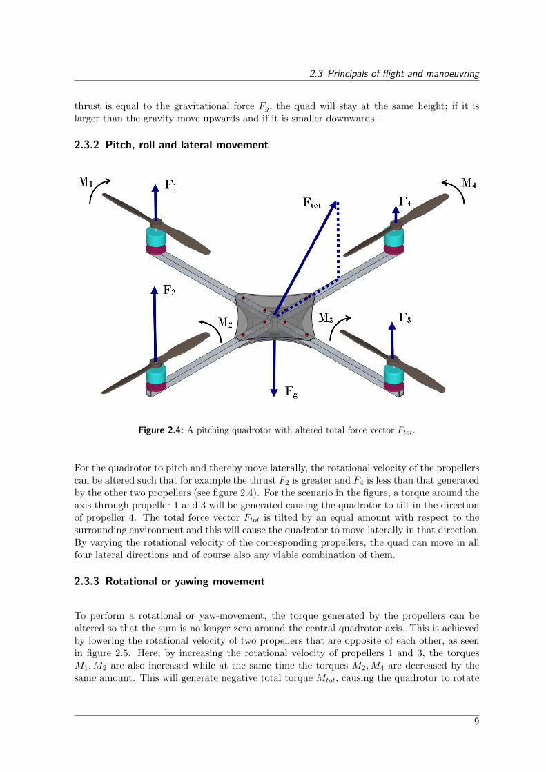
Figure 2.4: A pitching quadrotor with altered total force vector Ftot.
For the quadrotor to pitch and thereby move laterally, the rotational velocity of the propellerscan be altered such that for example the thrust F2 is greater and F4 is less than that generatedby the other two propellers (see figure 2.4). For the scenario in the figure, a torque around theaxis through propeller 1 and 3 will be generated causing the quadrotor to tilt in the directionof propeller 4. The total force vector Ftot is tilted by an equal amount with respect to thesurrounding environment and this will cause the quadrotor to move laterally in that direction.By varying the rotational velocity of the corresponding propellers, the quad can move in allfour lateral directions and of course also any viable combination of them.
2.3.3 Rotational or yawing movement
To perform a rotational or yaw-movement, the torque generated by the propellers can bealtered so that the sum is no longer zero around the central quadrotor axis. This is achievedby lowering the rotational velocity of two propellers that are opposite of each other, as seenin figure 2.5. Here, by increasing the rotational velocity of propellers 1 and 3, the torquesM1,M2 are also increased while at the same time the torques M2,M4 are decreased by thesame amount. This will generate negative total torque Mtot, causing the quadrotor to rotate
9

2 Quadrotor Platform
Figure 2.5: A rotating or yawing quadrotor.
around it’s center axis. Because the propellers are increased and decreased by the sameamount, the total force vector Ftot is not altered and the quadrotor will either stay at thesame altitude, or continue climbing/descending, while it is rotating.
10

3 Quadrotor Testbed
3.1 Introduction and specifications
To be able to effectively develop closed-loop position feedback controllers for the quadrotors(refereed to as agents), it was necessary to have a regulated environment that allows for quickimplementation and easy debugging of control algorithms. Furthermore, the testbed shouldallow a user of the system to implement different controllers with minimal effort and providefunctionality for conducting multi-agent control experiments. All of the experiments that wereconducted as a part of this thesis utilized the testbed, but it was also designed to provide theKTH Autmatic Control Laboratory with a platform for doing practical research in the multi-agent cooperative control area. To achieve this goal and as a major contribution to this thesis,a testbed for ground and aerial vehicles that is described in this chapter was developed. Asoftware and hardware framework was implemented, consisting self-developed program codeand applications, but also commercially available products that where integrated into thesystem.
As an overview, the testbed consist of three main subsystems plus the agents and theaccording interfaces. A positioning system is used to determine the agents position in space.A workstation computer running Microsoft Windows (referred to as ”controller PC”) is usedto run the main controller application and to connect all subsystems together. Finally, awireless link facilitates bi-directional communication between the agents and the controllerfor transmitting actuation commands to the agents, and telemetry data from the agents backto the controller. The following sections in this chapter will give a detailed description of alldifferent parts functionality, performance and technical data of the quadrotor testbed and theprocess that was undergone whilst designing it.
3.1.1 The closed-loop control system
To be able to accurately control each agent’s position in space, the three subsystems describedin the foregoing section where connected with the agents in a position-feedback control loopconfiguration. An overview of this loop and the parts that are involved is given in figure 3.1.
The controller PC is used to provide a platform for implementing different controller al-gorithms for cooperative control of the agents. To be able to calculate the desired actuationsignals for each individual agent, an interface is provided on the controller PC to access bothdata coming from the positioning system and also from the agents on-board sensors directlyvia the wireless link. After retrieving all necessary data, an actuation output command canbe calculated by the controller and transmitted to the agents. The wireless bi-directional link
11

3 Quadrotor Testbed
-
Figure 3.1: Overview of the testbed control feedback-loop.
serves this purpose of transmitting the commands to the agents while allowing them to freelymanoeuver in space without being constrained by a cable. It is implemented using TMoteSky wireless modules and more details can be found in section 3.3.
3.1.2 Agents - Quadrotors and other
For the tests that where performed as a part of this thesis, the quadrotor platform as describedin chapter 2 was used. However, the testbed can with minimal modification be used to controlother types of airborne or also grounded vehicles like radio-controlled small-scale car or truckmodels. This will allow for further research into multi-agent cooperative control with bothairborne and grounded agents.
For the agents to work with the testbed without further modifications, they have to pro-vide direct access to their actuation interface through a standard 3-pin radio-control servoconnector or a serial interface that allows to directly control these signals. Furthermore, theirsize and maximum velocity should be suited to the indoor space were the positioning systemis installed and they have to allow for the tags or reflective markers of the positioning systemto be installed on them.
12
3.2 Controller PC
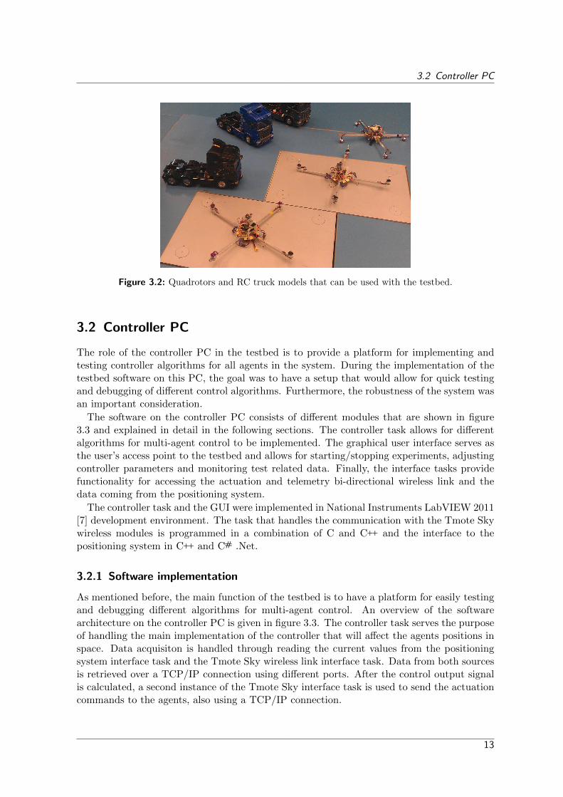
Figure 3.2: Quadrotors and RC truck models that can be used with the testbed.
3.2 Controller PC
The role of the controller PC in the testbed is to provide a platform for implementing andtesting controller algorithms for all agents in the system. During the implementation of thetestbed software on this PC, the goal was to have a setup that would allow for quick testingand debugging of different control algorithms. Furthermore, the robustness of the system wasan important consideration.
The software on the controller PC consists of different modules that are shown in figure3.3 and explained in detail in the following sections. The controller task allows for differentalgorithms for multi-agent control to be implemented. The graphical user interface serves asthe user’s access point to the testbed and allows for starting/stopping experiments, adjustingcontroller parameters and monitoring test related data. Finally, the interface tasks providefunctionality for accessing the actuation and telemetry bi-directional wireless link and thedata coming from the positioning system.
The controller task and the GUI were implemented in National Instruments LabVIEW 2011[7] development environment. The task that handles the communication with the Tmote Skywireless modules is programmed in a combination of C and C++ and the interface to thepositioning system in C++ and C# .Net.
3.2.1 Software implementation
As mentioned before, the main function of the testbed is to have a platform for easily testingand debugging different algorithms for multi-agent control. An overview of the softwarearchitecture on the controller PC is given in figure 3.3. The controller task serves the purposeof handling the main implementation of the controller that will affect the agents positions inspace. Data acquisiton is handled through reading the current values from the positioningsystem interface task and the Tmote Sky wireless link interface task. Data from both sourcesis retrieved over a TCP/IP connection using different ports. After the control output signalis calculated, a second instance of the Tmote Sky interface task is used to send the actuationcommands to the agents, also using a TCP/IP connection.
13

3 Quadrotor Testbed
Figure 3.3: Software architecture of the controller PC.
The graphical user interface (GUI) provides a user of the system with the possibility toquickly adjust different parameters that are relevant for the cooperative control experiments,such as varying the gain of the controllers that are used. Alongside this, the measurementstaken from the positioning system and the agents on-board sensors and are displayed, debug-ging functionality is provided and finally the possibility to manually control the actuationinputs of the agents.
For implementing the GUI and controller task, National Instruments LabVIEW 2011 in-tegrated development environment was chosen. LabVIEW (short for ”Laboratory VirtualInstrumentation Engineering Workbench”) provides the possibility for programming in graph-ical language named “G”. An extensive library of preprogrammed subroutines is included inthe distribution which simplifies tasks such as accessing the serial port or TCP/IP commu-nication. Further reasons for choosing LabVIEW were that development in the graphicalprogramming language is quick and that it inherently supports parallel execution of multipletasks, which is very useful when designing controllers for several vehicles at the same time.
A sample implementation of the GUI for controlling a quadrotor with four PID controllerfor pitch, roll, yaw and throttle is provided in figure [3.4]. When different control strategiessuch as LQG or MPC are used, the parameters that need to be adjusted vary and the GUIwill have to be adapted accordingly. With the sample implementation that is provided as areference framework and considering the easily learned user-friendly nature of the LabVIEWdevelopment environment, this will be an easy task for researchers working with the testbedin the future.
14

3.3 Wireless communication link
Figure 3.4: Sample implementation of LabVIEW GUI for controlling the four actuation in-puts of quadrotor with one PID controller each.
3.3 Wireless communication link
3.3.1 Tmotes technical description
The MoteIV Tmote Sky [8] is a wireless interface featuring a 2.4 GHz IEEE 802.15.4 Chipconwireless transceiver and an 8 MHz Texas Instruments MSP430 microcontroller on the samecircuit board. The microcontroller features USB, USART, SPI, I2C and GPIO interfacesfor connecting itself and the radio to other external components, such as the agents or thecontroller PC in case of the testbed.
For the testbed application, the TinyOS operating system [9] was chosen to be run on theTmote Sky module. TinyOS provides task scheduling, shared resource handling and severallayers of abstraction for accessing the underlying hardware components of the Tmote Skymodules. To create user-defined applications, they can be written in proprietary program-ming language named NesC. The syntax is similar to the C programming language, but theexecution model is event-driven instead of procedural as in C.
15

3 Quadrotor Testbed
Figure 3.5: The MoteIV Tmote Sky wireless module.
Manufacturer MoteIV Cooperation
Name Tmote Sky
Radio 2.4 Ghz IEEE 802.15.4 Chipcon
Radio throughput 250kbps
Radio range 50m indoors; 125m outdoors
Microcontroller TI MSP430 8MHz
Interfaces USB, SPI, USART, I2C, GPIO
Supply voltage 2.1 − 3.6 V
Dimensions 32 x 66 x 6 mm3
Weight 20 g
Table 3.1: Technical data for the Tmote Sky module.
3.3.2 Tmotes firmware implementation
To establish bi-directional communication between an agent and the controller computer,two Tmote modules where used on both the agent and on the computer (four in total). Oneof the modules on each side was used for sending and the other for receiving, facilitatingbi-directional communication. The reason for this is that the wireless radio module on theTmote Sky cannot receive and send and the same time, so with this configuration it was notnecessary to develop a scheduling algorithm, which would have been outside the scope of thisthesis.
For each of the four different Tmote Sky modules pictured in 3.6, a specific firmware wasdeveloped and run on top of the underlying TinyOS operating system layer on the module.One of the Tmote modules that is connected to the controller PC is programmed to receivedata over the wireless radio module. The data is then forwarder to the PC via virtual serialport from where it can be read from the serial forwarder application. The second Tmotemodule that is connected to the PC receives data from the controller task via another instanceof the serial forwarder and passes it on to the radio module. All data that is transmittedwirelessly is sent utilising the IEEE 802.15.4 protocol.
The first Tmote module that is located on the agent is programmed to receive data via theradio link and then pass it on to the UART serial output port, from where it can be fetchedby the agent’s control system. The second Tmote module receives data from its serial portand sends it back to the controller PC via the radio module. On the Tmote modules, the
16

3.4 Positioning systems
Figure 3.6: Four Tmote sky modules are used in a bi-directional communication channelbetween the controller PC and an agent.
radio and the UART serial port share a single physical connection to the micro-controller,so to make both work a scheduling algorithm was implemented which disables either of theshared resources when the other is active.
3.3.3 Tmote Sky - Controller PC interface
The Tmote Sky wireless radio module is connected to the controller PC via an USB connec-tion. The device drivers supplied by the manufacturer will emulate a virtual serial port onthe computer which can be accessed for reading data. To read the data from the virtual serialport, an application named “SerialForwarder” is provided as a part of the TinyOS distribu-tion. The serial forwarder accesses the virtual serial port provided by the Tmote module andforwards the data that was received wirelessly to a TCP/IP port. The port can be accessedfrom LabVIEW either on the same PC via the localhost or over a network connection. Theadvantage of this setup is that it allows for several motes to be used at the same time andalso that the serial forwarder will act as a buffer for incoming and outgoing data, so that nopackets are dropped.
3.4 Positioning systems
The positioning systems were used to measure the agents position in space. Two differentsystems are described in the following sections, where the Ubisense system was availableduring the whole time the thesis was performed, while the Qualisys system was only availablefor a limited period of time during a visit to the company’s headquarters in Gothenburg.
3.4.1 Ubisense system
The system is manufactured by Ubisense Ltd., United Kingdom [10] and consist of severalwall-mounted sensors and mobile tags that can be placed on the agents, as show in thefigure below. The sensors are mounted to the walls of the area in which the experimentsare performed and the agents to be located. All of the sensors are connected to each other
17

3 Quadrotor Testbed
through an Ethernet timing cable. One of the sensors will act as a master timing source forall others and distribute a clock signal to which the other sensors can synchronize themselves.A personal computer is in contact with all the sensors through a wired network connection.This computer gathers the calculated position data and provides a TCP/IP interface for otherclients (in this case the controller PC) that need to access the data.
Figure 3.7: Overview of the Ubisense positioning system.
To determine a tag’s position, the tag continuously emits an omnidirectional ultra-widebandpulse which is registered by the sensors. Upon receiving this signal, the sensor will determinethe angle-of-arrival and the time-of-arrival for this pulse. Since all sensors position is known,this data can then be used to calculate the three-dimensional position of the tag in space. Theposition data is given as x,y and z values in a right-handed Cartesian coordinate system. Inaddition to the ultra-wideband channel, a 2.4GHz telemetry channel is used to identify whichtag sent the pulse. Some technical data for the system in the given installation is provided intable 3.2 below.
Manufacturer Ubisense Ltd, UK
Sensor type Series 7000 IP
Tag type Series 7000 compact tag
UWB frequency 6 − 4 GHz
Telemetry channel 2.4 GHz
Positioning precision 10 cm
Maximum update rate 10 Hz
Tag dimensions 38 x 39 x 16.5 mm3
Tag weight 25 g
Table 3.2: Technical data for the Ubisense positioning system.
Ubisense interface
All of the Ubisense systems sensors are connected to a dedicated PC running proprietarysoftware, as described in section 3.4.1. This PC is connected to the controller computer via
18

3.4 Positioning systems
a TCP/IP wired Ethernet connection. The interface task is run on the controller computerand will make the data gathered by the Ubisense system accessible from within a LabVIEWenvironment. A dynamic link library (DLL) was implemented in the C# .Net frameworkand programming language. The DLL makes extensive use of the application programminginterface (API) provided by the Ubisense Ltd. company. The Ubisense system in its natureis event-driven, which means that the tag’s position is only updated when a tag is in motionand otherwise there will be no new position updates.
Because of this constraints, the interface task was designed to implement a buffer that willalways provide LabVIEW with the latest known position of a tag. Whenever a tag positionupdate is registered, the data will be written to an internal storage space from where it canbe read from other programs that need access to the data. Each tag is identified by a unique,12-digit number. From within the LabVIEW environment, the position data can be retrievedthrough calling the appropriate functions inside the DLL, which takes the tags identificationnumber as an argument.
3.4.2 Qualisys system
The Qualisys Motion Capturing system is a commercially available system designed for vision-based motion capturing for post-processing and data analyses but also for real-time position-ing. The system is manufactured by the Swedish company Qualisys AB based in Gothenburg.The system consists of a set of infra-red cameras that are placed around the area where theexperiments with the agents are performed, so that the whole area is in their line-of-sight.The cameras continuously emit a series of infra-red flashes, that allows them to detect severalretro-reflective ball shaped markers with a diameter of about 1 cm that reflect the infra-redlight back to the cameras. When the cameras detect a marker, the image of several cam-eras placed at different positions can be compared in order to recreate the three-dimensionalposition of the marker in space.
Figure 3.8: Overview of the Qualisys motion capturing system (http://www.qualisys.com).
A dedicated LabVIEW application was provided by the manufacturer of the Qualisys system.The application runs periodically from within the main controller application and will on eachiteration of the loop provide the controller with updated values for the agents position andorientation. For the LabVIEW interface to work, the Qualisys Track Manager applicationhas to be run in the background on either the controller PC itself or a separate PC that isconnected over a TCP/IP connection. This application communicates with the cameras andprocesses the data so that the agent’s positions can be determined.
19

3 Quadrotor Testbed
Manufacturer Qualisys AB, Gothenburg
Camera type Oqus 3
Marker type Retro-reflective ball-shaped marker
Positioning precision < 1 mm
Maximum update rate 500 Hz
Marker dimensions D = 1cm
Marker weight 3 - 5 g
Table 3.3: Technical data for the Qualisys positioning system.
Six degrees-of-freedom bodies
Alongside the ability to detect a single markers position in a world coordinate frame, theQualisys system can also be used to bundle four or more markers that are attached to anagent to form a rigid body. Within the Qualisys software package, a local coordinate systemcan be assigned to the bundled markers and the system can then also determine the threeorientation angles (pitch, roll and yaw) for the rigid body in real-time. This is a very usefulfeature since a lot of extra states of the agent can be measured without using additionalsensors, allowing for more precise control.
Figure 3.9: Screenshot from Qualisys Track Manger software highlighting the global (bot-tom) and local coordinate system of a 6 DoF body (upper right) alongside theorientation angles.
20

4 Quadrotor dynamic Model
4.1 Modelling
In this chapter, a dynamic model for the quadrotor platform described in chapter 2 is derived.A non-linear model will be given and a linearization performed that allow for linear controllerdesign in the following chapters. The derivation follows a method proposed by N. Michael,D. Mellinger et al. in [11] at University of Pennsylvania, however it is modified to accountfor the fact that in this case the desired value for the three orientation angles are used as aninput instead of using the rotational speed of the four motors as inputs. These desired valuesof the angles are fed to the internal controller of the quadrotor which will stabilize it at thedesired value.
4.2 Model derivation
Let us consider a world coordinate frame W and a body coordinate frame B that is attached tothe center of gravity of the quadrotor platform, as described in chapter 2. The two coordinateframes are shown in 4.1. Here, the positive direction of the body frame x-axis is chosen sothat it will point towards the forward flight direction of the quadrotor, while the positivey-axis will point to the left and the z-axis directly upwards if the quad is level (z-axis of worldand body frame parallel). The orientation of the quadrotor in the world frame is modelledby using Z-X-Y Euler angles which are given by ψ, the rotation around the z-axis, θ for therotation around the x-axis and φ for the y-axis rotation.
For transforming from body to world coordinate frame, the following rotational matrix isused (cθ = cosθ, sφ = sinθ and similarly for all other angles):
R =
cψcθ − sφsψsθ −cφsψ cψsθ + cθsφsψcθsψ + cψsφsθ cφcψ sψsθ + cψcθsφ−cφsθ sφ cφcθ
The forces acting on the center of mass of the quadrotor, which are the thrust generated bythe propellers (F1, .., F4) and gravity, can be modelled with the following equation:
m
xyz
=
00−mg
+R
00∑Fi
(4.1)
21

4 Quadrotor dynamic Model
ZW
YW
XW
ZB
YB
XB
Figure 4.1: The world coordinate frame W and the body frame B attached to the center ofgravity of the quadrotor.
After multiplication with R:
x =
∑Fim
(cosψ sin θ + cos θ sinφ sinψ) (4.2)
y =
∑Fim
(sinψ sin θ − cosψ cos θ sinφ) (4.3)
z =
∑Fim
cosφ cos θ − g (4.4)
Our inputs are the desired values of the three orientation angles. The dynamics betweem thedesired value and the actual value of an orientation are estimated as a first order transferfunction.
θ = kθ(θdes − θ) (4.5)
φ = kφ(φdes − φ) (4.6)
ψ = kψ(ψdes − ψ) (4.7)
The thrust Fi generated by a propeller depends on its rotational velocity ωi and is governedby the following equation [11]
Fi = kFω2i (4.8)
The total thrust is given by: ∑Fi = kF (ω2
1 + ω22 + ω2
3 + ω24) (4.9)
When a change in the desired value for θdes, φdes occurs, the quadrotor embedded controlsystem will change the rotational velocity of two opposing propellers (e.g. ω1, ω3), where it
22

4.2 Model derivation
increase one and decrease the other by equal amounts (4ω1 +4ω3 = 0). This increase anddecrease in ωi of the opposing propellers will be very small compared to the total rotationalvelocity. Thus, we can approximate that [4.8] and also [4.9] are linear for this small change.In conclusion, the total thrust will remain unchanged when manoeuvring (altering φ, θ, ψ) thequadcopter.
The final input variable for the model is chosen as ωdestot , which is the desired rotationalvelocity for all four propellers at level flight (θ, φ, dψdt = 0):
ωtot = ω1 = ω2 = ω3 = ω4 (4.10)
This corresponds to a certain total thrust amount which is given by:
∑Fi = 4kFω
2tot (4.11)
By following the conclusions above, it was shown that whilst both a change in θdes, φdes
and ωdestot will cause the propellers to rotate at different velocities, ωdestot can be used as anindependent input parameter if it is seen as the rotational velocity of all four propellers thatcorresponds to a certain total thrust amount at level flight. As was shown, this total thrustamount will not change if θ, φ, ψ change.
Finally, the dynamics between the desired and the actual rotational velocity are also esti-mated by a first order system [11]
ωtot = kω(ωdestot − ωtot) (4.12)
In summary, these are states that govern the quadrotor, where θdes, φdes, ψdes, ωdes areconsidered as inputs:
x =4kFω
2tot
m(cosψ sin θ + cos θ sinφ sinψ)
y =4kFω
2tot
m(sinψ sin θ − cosψ cos θ sinφ)
z =4kFω
2tot
mcosφ cos θ − g
θ = kθ(θdes − θ)
φ = kφ(φdes − φ)
ψ = kψ(ψdes − ψ)
ωtot = kω(ωdestot − ωtot)
23

4 Quadrotor dynamic Model
4.2.1 Non-linear model
The derivation presented in the foregoing section can be summarized in the following non-linear state-space equations, with u = (θdes, φdes, ψdes, ωdes) as the input vector:
x =
x
vx
y
vy
z
vz
θ
φ
ψ
ωtot
=
vx4kFω
2tot
m (cosψ sin θ + cos θ sinφ sinψ)
vy4kFω
2tot
m (sinψ sin θ − cosψ cos θ sinφ)
vz4kFω
2tot
m cosφ cos θ − gkθ(θ
des − θ)kφ(φdes − φ))
kψ(ψdes − ψ))
kω(ωdestot − ωtot)
4.2.2 Linearized model
To linearize the model, at first the equilibrium points of the system corresponding to x = 0have to be found.
x = 0 =
vx4kFω
2tot
m (cosψ sin θ + cos θ sinφ sinψ)
vy4kFω
2tot
m (sinψ sin θ − cosψ cos θ sinφ)
vz4kFω
2tot
m cosφ cos θ − gkθ(θ
des − θ)kφ(φdes − φ))
kψ(ψdes − ψ))
kω(ωdestot − ωtot)
The equilibrium points were chosen corresponding to the quadrotor being in level flight at acertain fixed altitude. Note that θ, φ have to be zero for the quadrotor to be in an equilibrium
24

4.2 Model derivation
state, while ψ can have any value (ψ = 0 was chosen for convenience).
x0 =
x0
v0x
y0
v0y
z0
v0z
θ0
φ0
ψ0
ω0tot
=
0
0
0
0
0
0
0
0
0√gm4kF
, u0 =
θ0ref
φ0ref
ψ0ref
ωdes,0
=
0
0
0
ω0tot
To get the linearised system, the partial derivative matrices A,B have to be derived, wherethe partial derivatives are taken with respect to x,u, respectively. A =
0 1 0 0 0 0 0 0 0 0
0 0 0 0 0 04kFω
2tot
m (cψcθ − sθsφsψ)4kFω
2tot
m (cθcφsψ)4kFω
2tot
m (−sψsθ + cθsφcψ) 8kFωtot
m (cψsθ + cθsφsψ)0 0 0 1 0 0 0 0 0 0
0 0 0 0 0 04kFω
2tot
m (sψcθ + cψsθsφ)4kFω
2tot
m (−cψcθcψ)4kFω
2tot
m (cψsθ + sψcθsψ) 8kFωtot
m (sψsθ − cψcθ sφ)0 0 0 0 0 1 0 0 0 0
0 0 0 0 0 04kFω
2tot
m (−cφsθ) 4kFω2tot
m (−sφcθ) 0 8kFωtot
m (cφcθ)0 0 0 0 0 0 −kθ 0 0 00 0 0 0 0 0 0 −kφ 0 00 0 0 0 0 0 0 0 −kψ 00 0 0 0 0 0 0 0 0 −kω
Evaluated at x0, A =
0 1 0 0 0 0 0 0 0 00 0 0 0 0 0 g 0 0 00 0 0 1 0 0 0 0 0 00 0 0 0 0 0 0 −g 0 00 0 0 0 0 1 0 0 0 0
0 0 0 0 0 0 0 0 0√
gm4kF
8kFm
0 0 0 0 0 0 −kθ 0 0 00 0 0 0 0 0 0 −kφ 0 00 0 0 0 0 0 0 0 −kψ 00 0 0 0 0 0 0 0 0 −kω
25

4 Quadrotor dynamic Model
B =
0 0 0 00 0 0 00 0 0 00 0 0 00 0 0 00 0 0 0kθ 0 0 00 kφ 0 00 0 kψ 00 0 0 kω
The linearized state-space system is now represented by the following equations:
x = x− x0 (4.13)
u = u− u0 (4.14)
˙x = Ax+Bu (4.15)
26

5 Controller design
In this chapter, the first section will deal with the synthesis and design of PID and LQ optimalcontrollers. A review of the general theory behind these control strategies will be given andthen the application to the quadrotors will be described in detail. In the second section of thischapter, the controllers will be evaluated by performing simulation in Matlab and Simulink,and by studying real-world results from using the quadrotor testbed.
The goal of the controllers described in the following sections is to stabilize the quadrotorat a given coordinate reference in space (x = xr, y = yr, z = zr) and also to move it there froman arbitrary zero state. Since these are the first experiments with this quadrotor platform, no”hard” goals in terms of performance specifications will be given, but instead safe and ratherslow-moving flight dynamics with conservative parameter tuning will be favoured. This willallow to avoid crashes and provide a baseline for further work with the intention to improvecontrol performance.
5.1 PID control
5.1.1 Theory
In PID or proportional-integral-derivative control the process variable y(t) that is to beregulated and the desired value or setpoint r(t) are subtracted to form the control errore(t) = y(t) − r(t). The PID controller uses this error as its input and calculates the outputu(t) by applying proportional, integral and derivative terms to the error and summing theresults.
u(t) = Kpe(r) +Ki
∫ t
0e(τ)dτ +Kd
d
dte(t) (5.1)
The proportional term will produce an output that is proportional to the error. However, pureproportional control will create a steady-state error or droop that can be countered throughusing an integral action. This term will sum the error over time and thereby eliminate thesteady-state error. The derivative term is used to slow the rate of change of the controlleroutput and thereby reduce the magnitude of an overshoot caused by the integral term. Theparameters Kp,Ki and Kd are used to tune the controller and adapt it to different processes.If a derivative or integral term is not desired, the appropriate constants can be set to zero andpure PD or PI controllers can be achieved. Different methods can be used to find suitablevalues for these parameters, such as for example Ziegler-Nichols [12].
27

5 Controller design
Figure 5.1: A PID controller in typical output-feedback configuration.
5.1.2 Design
As mentioned in the foregoing section, the goal was to control the quadrotors position inspace using the four inputs specified in chapter 4 (desired values for pitch, roll, yaw androtational velocity of the four propellers). If the yaw angle ψ is kept zero, so that the xB-and yB-axis of the quadrotor body frame is aligned with the corresponding axis of the globalcoordinate frame (xW , yW , figure 4.1), the desired value for the pitch angle θdes can be usedto control the quadrotors displacement on the xW -axis and similarly the roll angle φdes tocontrol the position on the yW -axis. This can be verified by comparing with the model givenin chapter 4. If there are only small deviations from level flight (such as when manoeuvringslowly), the linearized model from section 4.2.2 can be assumed to be valid and there will beno cross-coupling between either one of the input angles θdes, φdes and the displacement incorresponding output axis.
To fully control the quadrotor, four independent PID controllers are used: one for theheight, one for yaw angle and one for x- and y displacement, respectively. The yaw angle ψ isgoverned by a simple first-order differential equation that already contains an integral term(from the non-linear model in chapter 4).
ψ = kψ(ψref − ψ) (5.2)
Since there is already a integral term, a proportional controller of the following form is usedto control the yaw.
ψref (t) = u1(t) = K1eψ(t) (5.3)
The flight height or z-axis displacement of the quadrotor is governed by the following equations(θ, φ = 0).
z =4kFω
2tot
m− g (5.4)
ωtot = kω(ωdestot − ωtot) (5.5)
Here, a full PID controller with a constant additive term is used.
ωdestot (t) = u2(t) = ω0 +Kp,ωez(t) +Ki,ω
∫ t
0ez(τ)dτ +Kd,ω
d
dtez(t) (5.6)
The additive term ω0 is chosen so that it will cancel out the gravity g in equation 5.4. Theintegral term is used to account for long-term fluctuations in battery supply voltage of the
28

5.2 LQG control
quadrotor and the derivative term to smoothen the response to set-point changes and toreduce a possible overshoot.
The x- and y-axis dynamics of the quadrotor are given as follows (ψ = 0).
x =4kFω
2tot
msin θ (5.7)
y = −4kFω2tot
mcos θ sinφ (5.8)
θ = kθ(θdes − θ) (5.9)
φ = kφ(φdes − φ) (5.10)
Since an (dual-)integrator term is already present in differential function that connects inputand output, two PD controllers are used to control the movement of the quadrotor in thex- and y-directions, respectively. Again, the derivative term will ensure a smoother action.The proportional part of the controller will make the quadrotor tilt more in the respectivedirection the further it is away from the setpoint. Since it is not desirable for the quadrotorto tilt too much (it would move very fast or even crash if |θ, φ| > π
2 since there is no upwardslifting force any more), a saturation for θdes, φdes was implemented when programming thecontroller. The value of the upper and lower boundary is also a design parameter.
θdes(t) = u3(t) = Kp,θex(t) +Kd,θd
dtex(t) (5.11)
φdes(t) = u4(t) = Kp,φey(t) +Kd,φd
dtey(t) (5.12)
(eψ, ex, ey, ez are the errors in ψ, x, y, z, respectively)
5.2 LQG control
5.2.1 Theory
Linear-Quadratic-Gaussian or LQG control is the combination of Linear-Quadratic-Regulator(LQR) and a Kalman filter to estimate the full state from the measurable outputs. Boththe theory and design of the controller follow the derivation presented in [13]. To design acontroller, consider the following linear state-space representation of a plant where all statescan be measured.
x = Ax+Bu; (5.13)
y = x (5.14)
z = Gx+Hu; (5.15)
Here, x is the full state of the plant, y is the output, i.e. in this case all states can be measuredand z corresponds to the controlled output that controller should minimize. Now, the optimalcontroller can be found by minimizing the criteria as follows.
JLQR =
∫ ∞0
z(t)′Qz(t) + ρu′(t)Ru(t)dt (5.16)
29

5 Controller design
Now, since the whole state is known, an optimal state-feedback LQR controller is of the form
u = −Kx. (5.17)
Here, K is given by
K = (H ′QH + ρR)−1(B′P +H ′QG), (5.18)
where P is the positive-definite solution to the Algebraic Riccati Equation
A′P + PA+G′QG− (PB +G′QH)(H ′QH + ρR)−1(B′P +H ′QG) = 0. (5.19)
Since not all plants allow direct measurements of all states, let us now consider one with astate space model
x = Ax+Bu+ Bd; (5.20)
y = Cx+ n. (5.21)
Here, only the output y can be directly measured and the system is also affected by a dis-turbance d and the measurement noise n. To overcome this limitation, the non-measurablestates can be estimated using a Kalman filter and the optimal feedback matrix gain K canbe applied to the estimated state x, forming an LQG controller.
˙x = (A− LC −BK)x+ Ly (5.22)
u = −Kx (5.23)
To find the optimal state estimator, the matrix gain L that minimizes the expected value ofthe estimation error e = x− x has to be found:
JLQG = limt→∞
E[||e(t)||2] (5.24)
If d(t) and n(t) are zero-mean Gaussian noise processes with the following power spectrum
Sd(ω) = QN ,
Sn(w) = RN , ∀ω,
then the optimal estimator gain L is given by
L = PC ′R−1N . (5.25)
To determine P , the positive-definite solution to the Algebraic Riccati Equation
AP + PA′ + BQN B′ − PC ′R−1N CP = 0 (5.26)
has to be found.
30

5.2 LQG control
5.2.2 Design
To design an LQG controller, the linearized model that is presented in section 4.2.2 is used.
˙x = Ax+Bu (5.27)
The inputs are the desired values of three orientation angles and the throttle at the equilib-rium. The measurable output is chosen as the three position coordinates of the quadrotor’scenter of gravity in the world coordinate frame plus the three orientation angels.
y = Cx =
xyzθφψ
In practice this implicates that the orientation angles have to be measured, which can beachieved by either using the 6-Degrees-of-Freedom measuring functionality of the Qualisyspositioning system (section 3.4.2) or by retrieving the output of the quadrotors internal gy-roscope over the bi-directional wireless link (section 3.3).
To implement the controller and calculate the estimator and optimal feedback matrices,Matlab R2011 by MathWorks was used. The linearized model was programmed into Matlaband used as a parameter for the kalman() and lqr() functions that calculate the L and Kmatrices, respectively.
31


6 Evaluation and Results
In this chapter, an evaluation of the controllers and the testbed will be presented. Both thePID and LQR controllers introduced in chapter 5 were tested using the simulation softwareMathWorks Simulink [14]. The PID controller was also tested in a real-world environmentusing the actual quadrotor and testbed, but the LQR controller could not be tested due tolimited availability of the Qualisys system. All results that were obtained will be presentedin this chapter.
6.1 Simulation
6.1.1 PID
The PID controllers described in section 5.1 were implemented in Simulink together with thenon-linear model as seen in section 4.2.1. A block-diagram of the Simulink implementation isshown in figure 6.2. In the figure, the four independent PID controllers acting on each of theinputs can be seen. For lateral movement, the references are given in x and y coordinates,while the controller acts upon the corresponding orientation angels (θ and φ, respectively)that directly influences the desired output.
Figure 6.1: Simulink block diagram of the PID controllers and the non-linear quadrotormodel.
33
6 Evaluation and Results
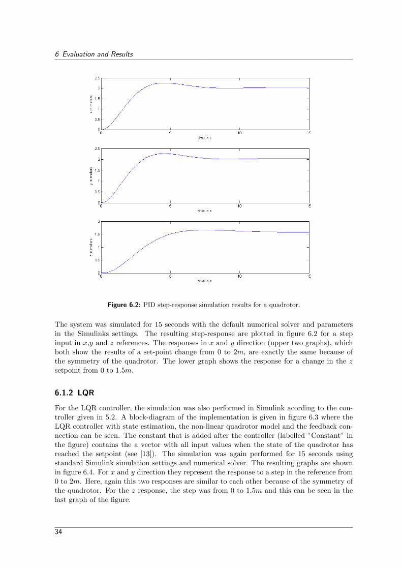
Figure 6.2: PID step-response simulation results for a quadrotor.
The system was simulated for 15 seconds with the default numerical solver and parametersin the Simulinks settings. The resulting step-response are plotted in figure 6.2 for a stepinput in x,y and z references. The responses in x and y direction (upper two graphs), whichboth show the results of a set-point change from 0 to 2m, are exactly the same because ofthe symmetry of the quadrotor. The lower graph shows the response for a change in the zsetpoint from 0 to 1.5m.
6.1.2 LQR
For the LQR controller, the simulation was also performed in Simulink acording to the con-troller given in 5.2. A block-diagram of the implementation is given in figure 6.3 where theLQR controller with state estimation, the non-linear quadrotor model and the feedback con-nection can be seen. The constant that is added after the controller (labelled ”Constant” inthe figure) contains the a vector with all input values when the state of the quadrotor hasreached the setpoint (see [13]). The simulation was again performed for 15 seconds usingstandard Simulink simulation settings and numerical solver. The resulting graphs are shownin figure 6.4. For x and y direction they represent the response to a step in the reference from0 to 2m. Here, again this two responses are similar to each other because of the symmetry ofthe quadrotor. For the z response, the step was from 0 to 1.5m and this can be seen in thelast graph of the figure.
34

6.1 Simulation
Figure 6.3: Simulink block diagram of the PID controllers and the non-linear quadrotormodel.
Figure 6.4: LQR step-response simulation results for a quadrotor.
35

6 Evaluation and Results
6.2 Testbed experiments
In this section, the results from performing experiments with the actual quadrotor platform(chapter 2) and testbed (chapter 3) will be presented. The control algorithm that was imple-ment was based on four PID controllers for each of the inputs of the quadrotor, as describedin section 5.1. The PID controllers where implemented in LabVIEW and the block-diagramof the code is given in 6.5. Three PID controllers for altitude and position control and onepure proportional controller for the yaw can be seen. The output of the PIDs for later con-troller have been limited by a saturation because otherwise the commanded input angle mightget too large, which will cause the quadrotor to tilt very far and thereby move too fast forsafe operation. For these experiments, the Qualisys positioning system (section 3.4.2) was
Figure 6.5: LabVIEW block diagram of the data acquisition from the Qualisys positioningsytem, PID controllers and the wireless actuation system interface.
used that allowed for direct measurement of the yaw angle. The position and angle data wasprocessed by the PID controllers and the actuation commands where sent over the wirelesslink (section 3.3) to the quadrotors. The resulting graphs that are directly captured from theQualisys data and imported into Matlab are shown in figure 6.6.
36

6.2 Testbed experiments
The three graphs shown in the figure represent the result of a step change in the set-pointof the reference value. For the upper graph, the reference in x was changed from 0 to 1m. Forthe middle graph, the y set-point was changed from −0.5m to 1m and the last graph showsa take-off procedure, where the quadrotor was sitting on the ground and the reference wasincreased from 0 to 1m, causing it to lift.
Figure 6.6: Quadrotor testbed step-response experiment results.
37


7 Conclusion and further work
In this thesis, a testbed for performing multi-agent control experiments with quadrotors wasdesigned. Parts of the testbed where a controller PC, a bi-directional wireless link and aninterface to a positioning system. The software on the controller PC that was implementedallows to access all data that is necessary for own control algorithms to implemented andthereby provides a framework for other people that want to perform practical experiments.It’s functionality was thoroughly tested and results from performing actual experiments arepresented as a part of this thesis. Furthermore, a model of the quadrotor was derived. Thismodel was implemented into simulation and the results show that it is a viable model thatallows to predict the behaviour of a the quadrotor in the testbed. LQR and PID controllerwhere designed based on the model that was derived. This controller where test using bothsimulation and the testbed, thereby further proving the functionality of the testbed.
For further work in this area and with the testbed, there are several recommendations tobe made:
• Cooperative control: Use the testbed to implement cooperative control between groundand aerial vehicles
• Parameter estimation: Estimation of the parameters that depend on the actual quadro-tor platform that is used in the model.
• LQR controller: Test the implementation of the LQR controller with the testbed
• Increase autonomicity: To make the quadrotor truly autonomous, the controllers forposition could be implemented directly on the quadrotor (instead of on the controllerPC) and only the desired set-point transmitted to them.
39


References
[1] Recco Avalanche Beacons: http://www.recco.com
[2] ArduCopter Platform: http://code.google.com/p/arducopter/
[3] JDrones Quadrotor: http://store.jdrones.com/
[4] Radio Controlled Aircraft: http://en.wikipedia.org/wiki/radio controlled aircraft/
[5] ArduPilot Mega: http://code.google.com/p/ardupilot-mega/
[6] Arduino Micro-controller: http://www.arduino.cc/
[7] Natinal Instruments LabVIEW 2011: http://www.ni.com/labview/
[8] Moteiv Tmote Sky Datasheet: Moteiv Cooperation, 2006
[9] TinyOS operating system: http://www.tinyos.net/
[10] Ubisense Ltd United Kingdom, Homepage: http://www.ubisense.net/en/
[11] ”The GRASP Multiple Micro UAV Testbed”: N.Michael, D.Mellinger, Q. Lindsey,V. Kumar, University of Pennsylvania 2005
[12] Ziegler-Nichols method: http://en.wikipedia.org/wiki/Ziegler-Nichols method
[13] ”Undergraduate lecture notes on LQG/LQR controller desing”: H.Hespanha, Universityof California, Santa Barbara, 2007
[14] MathWorks Simulink software: http://www.mathworks.com/products/simulink/
41