Mud on Your Face, Big Disgrace Vs. The Wisdom of Crowds

Macalester CollegeDigitalCommons@Macalester College

Honors Projects Economics Department

1-1-2012

Mud on Your Face, Big Disgrace Vs. The Wisdomof Crowds: Macroforecasters' Herding BehaviorOver TimeAdam J. FreedmanMacalester College, [email protected]

Follow this and additional works at: http://digitalcommons.macalester.edu/economics_honors_projects

This Honors Project is brought to you for free and open access by the Economics Department at DigitalCommons@Macalester College. It has beenaccepted for inclusion in Honors Projects by an authorized administrator of DigitalCommons@Macalester College. For more information, pleasecontact [email protected].

Recommended CitationFreedman, Adam J., "Mud on Your Face, Big Disgrace Vs. The Wisdom of Crowds: Macroforecasters' Herding Behavior Over Time"(2012). Honors Projects. Paper 50.http://digitalcommons.macalester.edu/economics_honors_projects/50

http://digitalcommons.macalester.edu?utm_source=digitalcommons.macalester.edu%2Feconomics_honors_projects%2F50&utm_medium=PDF&utm_campaign=PDFCoverPages

http://digitalcommons.macalester.edu/economics_honors_projects?utm_source=digitalcommons.macalester.edu%2Feconomics_honors_projects%2F50&utm_medium=PDF&utm_campaign=PDFCoverPages

http://digitalcommons.macalester.edu/economics?utm_source=digitalcommons.macalester.edu%2Feconomics_honors_projects%2F50&utm_medium=PDF&utm_campaign=PDFCoverPages



http://digitalcommons.macalester.edu/economics_honors_projects/50?utm_source=digitalcommons.macalester.edu%2Feconomics_honors_projects%2F50&utm_medium=PDF&utm_campaign=PDFCoverPages

mailto:[email protected]

Freedman 1

MUD ON YOUR FACE, BIG DISGRACE VS. THE WISDOM OF CROWDS: MACROFORECASTERS’ HERDING BEHAVIOR OVER TIME

Adam Freedman

Macalester College

Economics Honors 2012

Advisor: Pete Ferderer (Economics) Additional Readers: Gary Krueger (Economics) and Brooke Lea (Psychology)

ABSTRACT: I examine the herding behavior of macroeconomic forecasters for real GDP growth and unemployment rate forecasts. Although previous research has addressed cross-sectional differences in the propensity to herd, this paper explores changes in herding behavior over time. I present two theories. The first, based on Prospect Theory, predicts that a forecaster’s propensity to herd is inversely related to the size of his recent forecast error. The second theory predicts that the propensity to herd decreases when other forecasters make larger errors. The results reveal significant herding behavior and support for both theories. Implications for consumers of macroforecasts are addressed. Keywords: Macroforecasting, Behavioral Economics, Prospect Theory JEL Classifications: D03, E27, E32, E37, E47 ________________ Submitted: 6/22/2012 Acknowledgements: I would like to thank my professors, friends and family for their support, encouragement and assistance while writing this thesis. First, I would like to thank my advisor, Professor Ferderer, for his patience, insight and guidance throughout the project. He is a large part of my inspiration to study behavioral economics and to complete this project. Second, I would like to thank my readers, Professors Krueger and Lea, for their guidance and support while completing the project. Third, I would like to thank Professor Sarah West for her direction and support during the honors seminar. Fourth, I would like to thank my parents and sister for putting up with me elaborating my project any time they would listen and providing valuable feedback from a non-economics perspective, as well as providing non-academic support during the project and my four years at Macalester. Fifth, I would like to thank Kate Vermann for inspiring me to challenge myself at Macalester and continually helping me conquer academic and personal challenges. Sixth, I would like to thank my peers in the economics honors program and other students in the economics department that provided valuable insight and support while I was completing the project. Finally, I would like to thank my friends for their considerable patience and support as I worked to complete the project this year.

Freedman 2

1. Introduction Forecasts of GDP growth, inflation and other macroeconomic variables play an important

role in the economy because they influence the investment and production decisions of firms and

policy actions of central banks and other policy-makers. The success of firms and the ability of

policy-makers to promote economic stability and long-term growth are determined by their

access to accurate macroforecasts.

Unfortunately, studies have consistently found that economists do a poor job forecasting

macroeconomic variables (Zarnowitz, 1984; Zarnowitz, 1992; Zarnowitz & Braun, 1993; Schuh,

2001; Bauer, Eisenbeis, Waggoner & Zha, 2003). This is especially true around business cycle

turning points and other periods of significant economic change. For example, Schuh (2001) has

shown that all participants in the Survey of Professional Forecasts persistently under-predicted

GDP growth in the United States four years in a row between 1996 and 1999. Similarly, all

members of the Blue Chip panel of macroforecasters over predicted economic growth during the

Great Recession.

While the performance of individual forecasters has been poor, it has been shown in a

number of studies that there is a “wisdom of the crowd” in this field. That is, the mean forecast

across all forecasters, referred to as the “consensus forecast,” is more accurate than most

individual forecasts (Zarnowitz, 1984; Zarnowitz, 1992; Zarnowitz & Braun, 1993; Bauer,

Eisenbeis, Waggoner & Zha, 2003). For example, Bauer et al. (2003) find:

The Blue Chip Consensus Forecast consistently performs better than any of the individual

forecasters do. This result is a ‘reverse Lake Wobegon’ effect: none of the forecasters are

better than the average forecaster…There are superior forecasters, but no individual has

access to all of the independent information from all of the forecasts that is incorporated

into the consensus forecast. (p. 27)

Freedman 3

Other researchers theorize that the consensus forecast has superior accuracy due to the diversity

of individual estimation procedures and information used by macroforecasters to predict

macroeconomic variables (Page, 2004; Bates & Granger, 1969).

One explanation for the poor performance of individual macroeconomic forecasters is

that it is extremely difficult to produce accurate forecasts given the complexity of the

macroeconomic system and the inherent difficulty of predicting “shocks” which, by their very

nature, are unpredictable. An alternative explanation is that forecasters do not operate in a

vacuum and that interaction between them and additional motivations – beyond simple

maximization of accuracy – contribute to their poor track record. For instance, Lamont (2002)

argues that the presence of principal-agent problems can cause forecasters to use their forecasts

to manipulate beliefs about their ability. According to this view, forecasters sell their services

(forecasts) in monopolistically competitive markets where there is relatively free entry and exit

and potential for product differentiation. Moreover, the consumers in these markets (firms and

governments purchasing the forecasts, the “principals”) have imperfect information about the

quality of the forecasts (the “agents”). Given this market structure, it may be in the forecasters’

best interests to deliberately deviate from other forecasters to garner positive publicity for their

product. Alternatively, forecasters may mimic the forecasts of others (herd to the pack) in an

attempt to build a reputation as a consistently accurate forecaster among competitors (Laster,

Bennett & Geoum, 1999).

Previous studies have examined cross-sectional variation in herding and deviating

behavior. For instance Laster et al. (1999) show that independent forecasters deviate more from

other forecasters than non-independent forecasters (e.g., those affiliated with banks, industrial

firms, etc.) and conclude that the independent forecasters herd less because they place a greater

Freedman 4

value on publicity. Lamont (2002) provides evidence that more experienced forecasters herd less

than inexperienced ones and argues that this phenomenon illustrates forecasters’ recognition of

their true ability as they gain more experience. Gallo, Granger and Jeon (2002) find that

forecasters place a significant weight on the previous period consensus forecast when updating

their individual forecast.

In contrast to previous studies which focus on cross-sectional variation in forecasters’

propensity to herd, this thesis examines variations in herding behavior over time. I provide two

unique theories of herding behavior over time and test each. The first, which I refer to as the

Mud on Your Face Theory, contends that forecasters choose their herding behavior based on

their recent individual performance. Using Kahneman and Tversky’s Prospect Theory (1979;

1992), the theory predicts that forecasters herd less following large personal forecast errors

because they have suffered a loss to their reputation, become risk seeking and choose the riskier

strategy of deviating from other forecasters. Conversely, after forecasters forecast accurately,

they achieve reputational gains and become risk averse, and consequently decide to herd more.

Alternatively, the second theory, which I refer to as the Transitory Wisdom of Crowds,

suggests that herding behavior is driven by the recent performance of the consensus forecast.

This theory predicts that forecasters are more likely to herd to the consensus forecast if the

consensus has been accurate, and deviate from the consensus if it has been inaccurate.

I first address the previous macroforecasting and herding literature. I then provide two

theories that may explain changes in aggregate herding behavior over time. Next, I summarize

the data I use to evaluate these theories. Then I present the empirical model I use to measure

aggregate herding behavior and test my two theoretical models. I conclude by analyzing the

empirical results.

Freedman 5

2. Previous Literature 2.1. Macroforecasting

Macroforecasters aim to accurately predict macroeconomic variables such as GDP

growth, unemployment rates and interest rates. This information is used across many industries

to make business decisions regarding output, employment and investment as well as to guide

government policy.

Initially, researchers who studied the forecasting industry assumed that macroforecasters’

incentive structures only rewarded forecasting accuracy. That is, that they simply attempted to

minimize their mean forecast error. However, in the 1990s, researchers began to recognize other

factors that influence forecasts, collectively named “rational bias.” For example, researchers

have found that forecasters attempted to generate publicity for their firm to gain new clients by

differentiating their forecast from others (Batchelor & Dua, 1990; Lamont, 2002).

The wide demand for macroforecasting services has spurred the creation of numerous

forecasting firms. These forecasters are either directly employed by the consumer of their

forecasts (e.g., firms that forecast exclusively for specific banks, industrial organizations or

governments) or they are employed by a variety of consumers (e.g. independent forecasting

firms). The forecasting methods of these firms vary considerably, with some using formal

econometric models and others using less formal subjective methods. As an added performance

incentive, several publications that report survey panels of forecasts also provide a winner-take-

all award to the most accurate forecaster.1

Individually, macroforecasters have struggled to accurately predict macroeconomic

indicators. Although they are able to perform with relatively high success during periods of

1 These awards are generally given to a forecaster who is consistently accurate. For example, the Lawrence R. Klein award is given to the forecaster that has the smallest errors when forecasting real GDP growth, CPI inflation, the unemployment rate and the three-month Treasury bill rate from the Blue Chip Economic Indicators over a four-year period.

Freedman 6

consistent, predictable growth, they often struggle to identify turning points, such as transitions

from expansions to recessions (peaks) and vice versa (troughs).

2.2 The Benefits of Herding to Other Forecasters

A large portion of the macroforecasting literature has addressed herding, in which

forecasters choose to incorporate the previous forecasts of other forecasters into their updated

forecasts rather than relying exclusively on their private information. There are several benefits

of herding to other forecasters. Two benefits have been discussed at length in the literature:

taking advantage of the hard-won information of others (information-based herding) and

avoiding reputational losses due to deviating from the forecasts of others while incurring large

errors (reputation-based herding).

Information-based herding occurs when decision makers herd to take advantage of

others’ information (Bikhchandani, Hirshleifer & Welch, 1992; 1998). In Bikchandani et al.’s

theoretical model, they assume a set of sequential decision-makers that make binary affirmative

or negative decisions. These individuals make their respective decisions one after the other,

basing their choices on their private signals as well as the decisions of the previous individuals.

However, the decision-makers can only see the actions of the individuals before them

(observable actions) but cannot see their signals (unobservable signals). Additionally, none of

the individuals know the precision of their private signal or the precision of the private signals of

others.

The first mover only acts based on the information in his private signal because he does

not know the precision of his private signal. Depending on his unobservable signal, the second

mover then has the choice to either follow or deviate from the first mover. Specifically, if the

first mover’s observable action aligned with the second mover’s unobservable signal, the second

Freedman 7

mover would always choose the same decision as the first mover. If the first mover’s observable

action differed from the second mover’s unobservable signal, however, the second mover would

be indifferent between following the first mover or following his private signal. Based on their

model, Bikhchandani et al. contend that the third individual would likely follow the first two

actors if they chose the same option regardless of his private signal. If the first two actors chose

different options, however, he would be in the same position as the first mover and would move

based on his private signal. The authors define the case in which one individual and all

subsequent individuals follow the observable actions of the previous actors and ignore their

private signals as an “informational cascade.” Once the cascade begins and individuals stop

acting based on their private signals, the aggregation of private information in the decisions

stops. If they follow the correct signal and all subsequent actors make the right choice, it is

deemed a positive cascade; if not, it is a negative cascade.

Although their theory does not directly relate to forecasting, Bikhchandani et al. (1998)

tie the model into the general case of observing the summary statistic of individuals who have

already acted, similar to macroforecasting. They theorize that as long as the perceived precision

of the previous signals exceeds the decision-maker’s perception of the precision of his private

signal, the decision-maker will herd to the behavior of individuals before him. This situation

strongly resembles the case of macroforecasting, in which macroforecasters have the ability to

judge the recent success of their peers by comparing their peers’ recent forecasts to the actual

values of the variable being forecasted. However, Bikhchandani et al.’s model deviates from the

case of macroforecasting. Most notably, their model only allows for actors to make a binary

decision of herding or non-herding on a binary task. In macroforecasting, forecasters have the

option to choose the degree to which they herd, if at all.

Freedman 8

An alternative form of herding, reputation-based herding, occurs when individuals herd

to avoid falling far outside the group, rather than herding to take advantage of others’

information (Bikhchandani et al., 1998; Scharfstein & Stein, 1990). Bikhchandani et al.’s (1998)

theory is similar to that in Asch’s (1952) experiment, in which individuals knowingly answered a

question incorrectly for the sake of avoiding stigma due to deviating from the responses of

confederates in the experiment.2 In the terms of their informational cascade framework,

Bikhchandani et al. (1998) claim that individuals that act to avoid stigmatization are likely to

continue a negative cascade, even if their private signal precisely indicates otherwise.

Scharfstein and Stein (1990) add reputational considerations to the implied objective

function of decision-makers in Bikhchandani, Hirshleifer and Welch’s (1998) model. In

Scharfstein and Stein’s principal-agent model, investors are either “smart” due to their highly

informative signals that are highly correlated with market outcomes, or they are “dumb” and

receive uninformative, noisy signals. Scharfstein and Stein propose a “bright minds think alike”

assumption, suggesting that the “smart” forecasters will forecast in a tight pack around their

highly informative signals, and “dumb” forecasters will be randomly dispersed around the pack

of “smart” forecasters. Consequently, because neither the investors nor their clients know their

true ability and signal precision, the market’s perception of an investor’s ability is based on the

degree of similarity between an investor’s choices and other investors’ decisions.

In a framework of sequential decision-making similar to Bikhchandani et al. (1998),

Scharfstein and Stein (1990) argue that individuals are very likely to mimic the decisions of

2 Asch (1952) studied group conformity. In his experiment, subjects entered a room full of confederates, whom they were told were other participants. Each of the confederates and the subject were asked to identify the relative lengths of lines presented by the experimenter. Prior to the subject providing his or her opinion, all of the confederates misidentified the relative lengths of the lines. When it was the subject’s turn, they frequently gave the same erroneous response as the confederates. Asch attributed this result to the subject’s need to conform to the group; although he knew the correct answer, he gave an incorrect answer to be similar to the other group members.

Freedman 9

other investors for fear of exposing themselves as incompetent by predicting values that are far

from the group average. This type of reputation-based herding is also applicable to

macroforecasting, in which forecasters potentially have a high propensity to herd to the

consensus forecast in order to guarantee that, even if they are incorrect, they are wrong with the

other members of the group rather than being wrong alone.

Lamont (2002) empirically tested Scharfstein and Stein’s (1990) theory of reputation-

based herding among macroforecasters. Lamont examines two components that influence

herding behavior over macroforecasters’ life cycles. First, Lamont proposes the “tight-priors”

effect, which postulates that as a forecaster’s experience increases, that forecaster’s ability

becomes apparent and he is not able to deceive clients of his ability by following the herd.

Consequently, the theory predicts that forecasters herd less over their life cycles. Lamont also

considers the “far-to-fall” effect, in which a forecaster’s incentive to herd rises over his life cycle

due to the greater potential losses from deviating from the crowd later in the forecaster’s career

after he has achieved a strong reputation. Using annual macroforecasting data from Business

Week, Lamont finds that forecasters’ deviations from the consensus increase over their life cycle,

providing support for the tight-priors effect over the far-to-fall effect.3

Additional research has addressed other cross-sectional characteristics of

macroforecasters’ herding behavior. Ferderer, Pandey and Velatsianos (2005) built upon

Lamont’s (2002) work by comparing empirical evidence for information-based and reputation-

based herding among macroforecasters using macroforecast data from the Blue Chip Economic

Indicators data for real gross domestic product (GNP) growth, CPI inflation, the unemployment

3 Lamont (2002) provided additional support for this finding based on the comparative performance of human forecasters compared to econometric modelers. Specifically, he hypothesized that the theories would only apply to human forecasters whose forecasts are affected by reputational concerns, and that econometric modelers’ forecasts would not follow the same patterns due to their objective forecasting methods. As expected, he finds that the tight-priors effect holds only for human forecasters, and not econometric modelers.

Freedman 10

rate and short-term interest rates. After dividing the forecasters into winners and non-winners of

the Lawrence R. Klein Blue Chip Forecasting award, Ferderer et al. (2005) found support for

information-based herding. Specifically, they find that forecasters who win the award are

generally less likely to herd, showcasing the perceived strength of their private signal. When

they do herd, they are much more successful at efficiently incorporating information only from

other winners. Alternatively, they find that non-winners herd more over their life cycles as they

recognize the additional signal accuracy included in others’ forecasts compared to their private

signals. These non-winners are also less efficient when herding and herd to a larger group of less

accurate forecasters than to the forecasts of winners.

2.3 The Benefits of Deviating from Other Forecasters

Forecasters also benefit from deviating from the predictions of other forecasters.

Consider the market structure of forecasters as monopolistically competitive: the services

provided by forecasters are highly differentiated, there is free exit and entry into the market,

there are many consumers and forecasters in the market, and forecasters have some control over

the price of their services. Consequently, forecasters are incentivized to differentiate their

product by offering the lone best product to maximize the price they can charge for their

services. Batchelor and Dua (1990) conducted one of the seminal studies on forecast

differentiation and found that a select group of forecasters consistently provided overly

optimistic or pessimistic forecasts over the sample period and concluded that this strategy of

providing extreme forecasts was used to differentiate their product. Subsequent research has

evaluated how forecasters’ decisions to herd and deviate from other forecasters vary across

different types of forecasters based on the incentive structure that comprises each forecaster’s

unique reward function (Laster et al., 1999).

Freedman 11

Macroforecasters are incentivized to both maximize their individual accuracy and

generate positive publicity for their firm (Batchelor & Dua, 1990; Hong, Page & Riolo, 2011;

Laster et al., 1999).4 In most cases, forecasters are influenced by both incentives and choose

their herding behavior as a combination of the two, based on the preferences of their clients.

“Profit maximisation by forecasters may involve sacrificing some accuracy in the interests of

producing a distinctive product. So it may be optimal for forecasters to publish technically

irrational forecasts in a commercial forecasting environment” (Batchelor and Dua, 1990).

In the first incentive structure, forecasters are compensated based only on their individual

accuracy of predicting an economic indicator. If they predict correctly, regardless of how the

other forecasters perform, they will receive a high payoff. This compensation framework is

likely to dominate among institutional forecasters, such as banks or manufacturing firms, in

which the forecasters already have their clients and are forecasting for internal purposes.

In contrast, forecasters are also rewarded based on their performance relative to the rest

of the group and the consequent publicity they generate for their firm. If they predict correctly,

their compensation is inversely related to the number of other forecasters who also predict

correctly (i.e. compensation is highest when a forecaster is correct alone and lower when he and

many other forecasters are all correct). Consequently, this incentive structure rewards

forecasters for deviating from the group and can cause them to forgo potential accuracy for the

potential positive publicity achieved by being correct and different from all other forecasters.

This compensation framework is more likely to dominate the objective functions of aspiring

forecasters who are looking for new clients and therefore are trying to differentiate themselves

4 Hong et al. (2011) refer to the incentive structure that rewards individual accuracy as “individual-based incentives” and the incentive structure that rewards generating publicity for one’s firm as “market-based incentives”. I exclude this terminology to simplify my analysis of these incentive structures.

Freedman 12

from the herd by generating publicity for their services (Batchelor & Dua, 1990; Hong et al.,

2011; Laster, Bennett and Geoum, 1999).

It is important to note that an individual forecaster’s utility function generally includes

incentives that reward his individual accuracy, as well as incentives that reward him for

generating positive publicity for his firm, based on his personal preferences as well as the

preferences of his clients. Consequently, forecasters attempt to maximize their utility (wages)

subject to the constraints of their market structure. Laster et al. (1999) studied systematic

differences between the market structures of different types of forecasters that arise from the

demands of their clients.

Laster et al. empirically examined the relative importance of accuracy-driven and

publicity-driven incentives for different types of forecasters. Specifically, Laster et al. employ a

framework in which a forecaster’s wage is determined by his accuracy and by the publicity he

generates for his firm by differentiating his product from his competitors. In Laster et al.’s

model, the users of forecasts are divided into two groups: “intensive” users that consistently

follow forecasts to guide business decisions, and “occasional” users that only use forecasts

periodically. Laster et al. theorize that intensive users likely monitor a set group of forecasts

each period. Consequently, forecasters that cater to these users are more incentivized to produce

consistently accurate forecasts than to generate publicity for their product. Alternatively,

occasional users tend to choose a forecaster based on his recent performance. Consequently,

forecasters that cater to occasional users are incentivized to deviate from other forecasters to

differentiate their product while also attempting to maximize accuracy, but to a lesser degree

than forecasters that already serve intensive users.

Freedman 13

In their paper, Laster et al. (1999) analyze the cross sectional differences in herding

behavior of different types of forecasters. One group, which consists of banks, econometric

modelers, industrial firms and security firms, caters to “intensive users” of forecasts.

Alternatively, independent forecasters target “occasional users” of forecasts. Therefore, the

utility function of the first group, which caters to intensive users, consists of a compensation

structure that rewards these forecasters for their consistent individual accuracy more than

generating publicity for their firm, as their customers are more interested in their consistent

success than occasionally being the most accurate forecaster. In contrast, the second group,

which consists of independent forecasters, is rewarded more for generating publicity for their

firm than being consistently accurate. This strategy is used by independent forecasters to

differentiate themselves from their competitors to gain new “occasional” users. These

independent forecasters may gain publicity from time to time by choosing to deviate from the

consensus, and thus will be less accurate on average. However, independent forecasters are

willing to accept long-term inaccuracy to periodically gain occasional users. Laster et al.’s

(1999) results support their theory, indicating that independent forecasters deviate most from the

consensus forecast.

2.4 The Value of the Consensus Forecast

2.4.1 Accuracy of the Consensus

After extensive research into the performance of individual forecasters, studies shifted

their focus to the performance of the consensus forecast, a simple average of all the individual

forecasts. Researchers hypothesized that the consensus forecast would be more accurate than

individual forecasts because it aggregates the diverse estimation procedures of all the individuals

included in the consensus. Consequently, they predicted that individual forecasters’ estimation

Freedman 14

biases would cancel to reveal the true value of the indicator in the consensus. Studies using the

Blue Chip Economic Indicators consistently find evidence of the “wisdom of crowds” in

macroforecasting, in which the ‘crowd’ (the consensus forecast) consistently if not always

outperforms the best individual forecaster (Zarnowitz, 1984; Zarnowitz, 1992; Zarnowitz &

Braun, 1993; Bauer, Eisenbeis, Waggoner & Zha, 2003).5 Additionally, recent studies of

herding have found that when macroforecasters choose to herd, they generally herd to the

consensus forecast (Ferderer et al., 2005).

2.4.2 The Value of Diversity6

Researchers theorize that the consensus forecast outperforms individual forecasts due to

the cognitive (and consequently, model specification) diversity of forecasters. For instance, Page

(2007) shows that group success is based on two factors: individual ability and the components

of individual diversity (perspective, interpretation, heuristic and predictive model diversity). 7

Assuming that a sample is drawn from a large group of smart and diverse individuals that are

working on a difficult task, his theory predicts that a group of randomly selected decision-makers

will generally outperform a group of the best-performing individuals on problem-solving tasks.

Based on this theory, he argues that the diversity of a group drives the group’s performance as

much as their individual abilities.

5 For a review of the consensus forecasting literature, see Clemen (1989). It is important to note that, although individual performance varies significantly from period to period, in the long run there are high-performance and low-performance individual forecasters (Schuh, 2001). 6 Although the core of diversity literature presented in this paper is drawn from Page’s (2007) book, the importance of diversity and the wisdom of crowds has been addressed widely the in statistics and economics literature. One of the first studies was conducted by Galton (1907), in which he calculated the consensus estimate of the weight of a steer at a county fair in England. More recently, Bates and Granger (1969) advocated for ideological diversity in forecasts to maximize the collective value of a consensus forecast. For a complete review of the wisdom of crowds literature, see Surowiecki (2004). 7 He claims that each individual has unique approaches to characterizing situations and challenges (perspective diversity), organizing their perspectives (interpretation diversity), developing resolutions to problems (heuristic diversity) and modeling cause and effect (predictive model diversity).

Freedman 15

Page and Hong (2004) empirically test this theory using computer-generated actors that

have constant perspectives but different individual abilities and problem-solving heuristics.

After testing each individual for baseline performance on a task in which the individuals were

programmed to find the maximum value of a random value function, they assembled teams of 10

and 20 from two pools: top-performers and randomly selected agents. These teams worked

together by using their heuristics to maximize a local value, such that after the previous actor

could not find a higher value, the next individual would take over. Eventually, when all the

agents became stuck on the same point, the exercise would stop. Page and Hong found that, on

the whole, teams of randomly selected actors had considerably more heuristic diversity than

teams of top performers and on average performed better than the teams of top performers.

One of the conclusions Page draws from this result is that the whole is greater than the

sum of its parts: collectively, a diverse group can do more than what all the individual group

members could do separately. For example, if one individual possesses one approach to a unique

problem and another person has a different approach, individually they may not be able to solve

a more complicated problem. However, if they work together and combine their problem

solving techniques (heuristics), they are more likely to be able to solve the problem. Page

explains this outcome using an analogy of a toolbox: although all the individual tools in a

toolbox may only be able to accomplish simple tasks such as hammering a nail or screwing a

screw, together, through their collective abilities, they are able to accomplish much greater tasks

such as building a tree house (Page, 2007).

Page applies these findings to the predictive ability of teams, and concludes that as a

crowd’s diversity increases, the error of the crowd’s consensus forecast decreases. He bases this

finding on what he terms the “Diversity Prediction Theorem”:

Freedman 16

!!

(!! − !!,!)!!!!! = !!

[!!

!!,! − !!,!)! − !!

[!!

(!!,! − !!)!]!!!!

!!!!

!!!!

!!!! (1)

Collective Error = Average Individual Error – Prediction Diversity

The theorem states that the average consensus squared error (!!

(!!!! !! − !!)!: average squared

deviations of the consensus forecast (!!) from the actual (y!,!) outcome for periods 1 through N)

equals the average individual squared error (!!

[!!

y!,!-‐y!,!)!!!!!

!!!! : average squared

difference between forecaster i through !’s forecasts (!!,!) and the actual forecasts (!!,!) for

periods 1 through N) minus the prediction diversity (!!

[!!

(!!,! − !!)!]!!!!

!!!! : average squared

differences between forecaster i through !’s forecasts (!!,!) and the consensus forecasts (!!) for

periods 1 through N). Using this theorem, he extends his previous conclusions to predictive

tasks, finding that diversity is of equal importance to individual ability. In these cases, he

highlights the “Projection Property”: when various people base their predictive models on

different variables and they have the same perception of the problem they are solving, the

correctness of their predictions will generally be negatively correlated, and they will cancel each

others’ errors. As diversity in the group grows, these benefits become multiplicative due to the

coverage of additional variables and the development of interactive effects in the consensus. In

terms of macroforecasting, Page’s framework explains the relative success of the consensus

forecast compared to all individual forecasters.

Herding presents a significant challenge to Page’s theory of the benefits of diversity.

Herding diminishes the cognitive diversity of a crowd because some proportion of the group

ignores their private information and their personal models of interpreting those signals. Page

(2007) recognizes the negative impact of herding on diversity, and consequently theorizes that to

maximize cognitive diversity, individuals should not be able to see others’ actions. This may not

Freedman 17

be possible in real-life environments in which forecasters have the ability to herd by

incorporating the consensus forecast from the previous period into their current-period forecast.

2.5 Addition to Literature

Previous studies of macroforecaster herding have focused on differences across

forecasters that affect their propensity to herd. The findings presented in this literature are very

important and necessary to control for when conducting empirical tests. However, in this study I

evaluate a group of forecasters’ average propensity to herd over time. I attempt to explain

systematic variations in forecasters’ herding behavior over time based on factors such as

business cycles and the accuracy of the consensus forecast.

3. Theory

As outlined above, macroeconomic forecasters are motivated by two primary

considerations: accuracy and publicity. Forecasters aim to be close to the actual value of the

variable they are predicting. However, their efforts to be accurate are mitigated by their desire to

receive publicity, which rewards them for being the lone correct forecaster. This motivates them

to differentiate their product from those of their competitors. Each month, forecasters learn the

predictions of other forecasters from the previous month through publications such as the Blue

Chip Macroeconomic Indicators. After receiving this information, forecasters then choose the

degree to which they incorporate the consensus forecast from the previous period into their

revised forecast based on their incentive structure and the public information available to them.

In this section I outline two theories that can explain fluctuations in macroforecasters’

herding behavior over time. The first, which I refer to as the Mud on Your Face theory, uses

Prospect Theory (Kahneman & Tversky, 1979; 1992) to predict how forecasters’ recent

individual accuracy influences their herding behavior. This theory predicts that, during periods

Freedman 18

in which forecasters are performing well (e.g., stable moderate expansionary stages of the

business cycle when there are few adverse shocks) and are experiencing reputational gains, they

will choose to herd more. However, during periods in which their individual accuracy decreases

(e.g., recessionary periods following a large negative shock or significant expansionary periods

following large positive shocks) and they are experiencing reputational losses, the theory

predicts that forecasters will choose to deviate more from the consensus. The key factor driving

this result is that forecasters’ risk preferences are determined by whether they are operating in

the domain of reputational gains or losses: during periods of reputational gains, forecasters are

risk averse which causes them to herd more. Alternatively, during periods of reputational losses,

forecasters are risk taking which causes them to herd less.

A second theory, The Theory of the Transitory Wisdom of Crowds, utilizes the recent

accuracy of the consensus forecast to predict macroforecasters’ herding decisions and is based on

information-based herding theory. The theory predicts that if the consensus forecast has been

accurate recently, forecasters will perceive that it contains valuable information and will choose

to herd more to increase the accuracy of their forecasts. Alternatively, if the consensus forecast

has been inaccurate, forecasters will choose not to decrease their herding behavior because they

perceive that the consensus does not contain valuable information.

3.1. Mud on Your Face Theory

One potential explanation of changes in herding behavior over time is how forecasters

respond to variations within the business cycle. Zarnowitz and Lambros (1987) find that the

variance of macroforecasts increases significantly following large negative or positive stochastic

shocks that force the macroeconomy into recession or rapid expansion, respectively. Zarnowitz

and Lambros theorize that this phenomenon occurs due to increased macroeconomic uncertainty

Freedman 19

during these periods. Kahneman and Tversky’s (1979; 1992) Prospect Theory provides a

potential alternative explanation for this outcome.

3.1.1. Prospect Theory

Kahneman and Tversky (1979; 1992) address agent decision-making under conditions of

uncertainty. They contest that actors begin at a reference point, having achieved either gains or

losses, which determines their current utility. Their future utility is determined by their relative

gains or losses to wealth or reputation from their current position.8 Kahneman and Tversky

derive this behavior from the incorporation of dynamic risk preferences into actors’ decision-

making processes based on their changes to states of wealth (see Figure 1). They theorize that

when an individual’s reference point is positive and they have been achieving gains (on the

positive side of the x-axis; for example, Point A), they are risk averse due to the concavity of

their utility function. Due to the concavity of their utility function during these periods of gains,

Prospect Theory predicts that the disutility of a loss significantly exceeds the utility gains of a

comparable gain. Alternatively, when they are in the loss domain (on the negative side of the x-

axis; for example, Point B), they are risk averse due to the convexity of their utility function.

Consequently, due to the convexity of their utility function during periods of losses, the utility of

a gain significantly exceeds the disutility of a comparable loss. 9

For example, consider a bettor’s betting behavior at the end of the day at the racetrack.

By the end of the day, most bettors are in the loss territory due to the racetrack’s advantage.

8 Alternatively, expected-utility theory predicts that individuals will rationally evaluate the probability of each outcome and make a decision on how to act based on their expected outcome regardless of their reference point: Expected Value = Prob (x1)*Expected Value (x1) + Prob (x2)*Expected Value (x2) … Prob (xn)*Expected Value (xn). Expected-utility theory predicts that a decision maker’s final utility is determined by his final position on his value function, as opposed to his change in position on the value function. 9 The other key finding of Prospect Theory is that individuals will overestimate the likelihood of unlikely outcomes and underestimate the likelihood of likely outcomes. For example, for low likelihood events, individuals are keen on making long shot bets and purchasing insurance, even though the possibility of winning the lottery or using the insurance is very low. However, individuals generally overweight the difference in likelihoods for highly probable versus certain events.

Freedman 20

Consequently, bettors attempt to return to gains territory by making bigger bets on long shot

horses, similar to publicity seeking forecasters driven by publicity-rewarding incentives.

Camerer (1998, pg. 7) contends, “These bettors really prefer longshots because a small longshot

bet can generate a large enough profit to cover their earlier losses, enabling them to break even.”

This result illustrates the dominance of prospect theory in human behavior, in that the bettor is

willing to forgo probable additional losses to generate the small possibility that his long shot bet

will result in a large payoff.

3.1.2. Application to Macroforecasters

Prior theoretical models of forecaster behavior assume risk neutrality (Scharfstein &

Stein, 1990; Laster, Bennett & Geoum, 1999). Consequently, to predict the implications of

Prospect Theory for macroforecaster herding, we must theorize the implications of dynamic risk

preferences on herding behavior.

Previous empirical studies find that forecasters consistently perform better during periods

of stable and predictable economic activity, in which large macroeconomic shocks do not occur

(Schuh, 2001; Zarnowitz, 1984; Zarnowitz, 1992; Zarnowitz & Braun, 1993). Lamont’s far-to-

fall effect may explain why forecasters herd more during these periods: “As a forecasters’ wages

and reputation rise over time, his reputation becomes a more valuable asset to be protected…and

herding increases” (1995). Although Lamont’s theory is designed to explain behavior over the

career of a macroeconomic forecaster, it provides useful insight into the short-run decisions of

individual macroforecasters as their reputation varies over the business cycle. During periods of

reputational gains, forecasters are likely risk averse and herd to avoid reputational losses from

inaccurate forecasts. Because their reputation is already high and the utility over gains is

concave, the additional utility generated from an even better reputation is small. If they herd and

Freedman 21

predict incorrectly, they will not be incorrect alone and suffer from a significant loss of

reputation. Prospect Theory’s predicted risk aversion strengthens Lamont’s far-to-fall effect,

which is hypothesized under risk neutrality.10

For example, consider Figure 2. This provides an example of a forecaster’s position on

his value function (y-axis) after a period of sustained, steady, low-shock growth, in which he is

in gains territory at point X (x-axis). He faces a decision, to herd more or less. If he herds more,

he reduces his range of possible reputational levels for the next period. On the one hand,

increased herding reduces his potential to stand out and experience a large gain in reputation. On

the other hand, increased herding protects him from a large drop in reputation by being wrong

alone. I assume that by herding, he has a .5 probability of either experiencing small gains or

small losses from either becoming more or less accurate (range A-A’), yielding an expected

value slightly below his current value (Expected Value Herding). If he herds less, however, he

faces a wider range of potential outcomes (assuming .5 probability of gains or losses, range B-

B’), yielding an expected value further below his current value, and below his expected value if

they were to herd (Expected Value Deviation). Due to the dynamic nature of his risk

preferences, his perceived potential losses are significantly greater than his perceived potential

gains of deviating from the consensus forecast, which results in herding behavior.

Alternatively, during periods following large unpredictable macroeconomic shocks,

forecasters will perform worse and face reputational losses. Here, herding protects him against

further losses in reputation but his potential changes in utility are small. On the other hand, by

herding less the forecaster increases the possibility of receiving positive publicity, which

10 Lamont also addresses a competing theory, called the “tight priors effect,” in which a forecaster’s ability to herd decreases throughout their career decreases as their clients become more aware of their actual ability. Similarly to the far-to-fall effect, the tight priors effect is based on the progression of a forecaster’s herding behavior over the career. However, there it is not applicable to the current case because I do not address the perception of a forecaster’s ability over his career.

Freedman 22

increases his reputation and, due to the convexity of his utility function, provides him with large

positive marginal utility. For example, consider Figure 3. After a large macroeconomic shock, a

forecaster is in loss territory at point X (x-axis). Similar to the forecaster in gains territory in the

previous example, he also can choose to either herd or deviate from the lagged consensus. If he

herds, he can reduce the uncertainty of his utility in the next period by likely remaining near his

current position, assuming a .5 probability of experiencing small gains or small losses (range A-

A’). This option yields an expected value slightly above his current value (Expected Value

Herding). If he deviates from the lagged consensus, however, his expected value (Expected

Value Deviation) is significantly higher than both his current value and his expected value if he

were to herd. This is due to the wider range of potential outcomes and the convexity of his

utility function (assuming .5 probability of gains or losses, range B-B’). In this case, the

forecaster faces disincentives to herd because the perceived potential gains of deviating from the

consensus forecast outweigh the potential losses in the individual forecaster’s value function.

The Mud on Your Face Theory predicts that when a forecaster is performing well and

experiencing reputational gains, he will herd more. However, following poor performance and

consequent reputational losses, he will herd less. The two key assumptions that generate this

prediction are that (1) increased herding reduces the range of possible changes to reputation and

(2) there is a concave relationship between utility and reputation in the domain of gains and a

convex one in the domain of losses.

3.2. The Transitory Wisdom of Crowds

An alternative theory of macroforecaster herding behavior contends that macroforecasters

choose their herding behavior based on the accuracy of the consensus forecast over the past

several periods. For example, consider a multi-period model (shown in Figures 4a and 4b). In

Freedman 23

t = 0, individuals are in information isolation and are unable to herd to the consensus. In terms

of macroforecasters, this isolation occurs when they have no information about their peers’

forecasts, likely at the beginning of a new forecasting horizon. Consequently, they rely on their

private signals, which maximize the information diversity included in the consensus. Page

(2007) theorizes that this high level of diversity should maximize the accuracy of the consensus

forecast. In t =1, forecasters can observe the consensus forecast and recognize that it was more

accurate than their individual forecasts. Therefore, they choose to incorporate the lagged

consensus into their forecast revision to encompass the additional information included in it.

This diminishes the diversity and accuracy of the consensus forecast but increasing the accuracy

of their individual forecasts. In period t = 2, forecasters begin to recognize the diminishing

accuracy of the consensus and realize that their independent forecasts may be more accurate due

to the lack of diverse information contained in the consensus. Consequently, they diminish the

weight they place on the lagged consensus in their current period forecast. In period t = 3, as the

forecasters decrease the weight they place on the consensus, the diversity of information

included in and accuracy of the consensus begins to rise again, and once it exceeds the accuracy

of most forecasters, they will begin herding again, resulting in a cyclical pattern (See Figures 4a

and 4b). Due to the frequent updates published, the forecasters cannot sufficiently judge the

accuracy of the consensus from period to period. Consequently, herding behavior would

continue to fluctuate and not converge to an equilibrium value.

3.3. Summary of Theoretical Predictions

The Mud on Your Face theory and the Theory of the Transitory Wisdom of Crowds

provide identical hypotheses regarding herding behavior during periods in which recent

individual and consensus forecasts have been accurate or inaccurate. During periods in which

Freedman 24

the individual’s forecast and the consensus forecast have both been accurate, both models predict

that forecasters are motivated to engage in herding behavior and place a high weight on the

lagged consensus forecast when revising their forecast. Alternatively, during periods in which

both the individual’s forecast and the consensus forecast have been inaccurate, both theories

predict that the individual will deviate from the lagged consensus forecast.

However, during periods in which the accuracy of the individual’s forecast and the

consensus forecast have differed, the theories make different predictions. When the individual’s

forecast has been accurate and the consensus forecast has been inaccurate, the Mud on Your Face

theory predicts that the forecaster will herd more and the Transitory Wisdom of Crowds theory

predicts that the forecaster will deviate from the consensus. When the individual’s forecast has

been inaccurate and the consensus forecast has been accurate, the Mud on Your Face theory

predicts that the forecaster will herd less and the Transitory Wisdom of Crowds theory predicts

that the forecaster will herd more. These predictions are summarized in Table I.

4. Data / Summary Statistics 4.1 Conceptual Model

To evaluate the predicted theories, we aim to measure the components of the average

forecaster’s herding behavior. Herding in macroforecasting occurs when a forecaster is revising

his forecast and instead of only using his previous period forecast and new information about the

state of the macroeconomy, he also places some weight on the consensus forecast from the

previous period. In this thesis, I aim to estimate the average weight forecasters place on the

lagged consensus when making their current period forecast, what factors contribute to their

decision, and what other information they use when updating their forecast. The Mud on Your

Face theory suggests that the propensity to herd is inversely related to the forecaster’s recent

forecast error. The Theory of the Transitory Wisdom of Crowds proposes they choose based on

Freedman 25

the recent accuracy of the consensus forecast.11

4.2. Ideal Data

The ideal macroforecasting data for this analysis would cover a long period that includes

several business cycles. The data would include a balanced set of macroforecasters, all of who

would have forecasted in every period. Each of the forecasters would employ the same

forecasting staff across time to limit intra-forecaster firm heterogeneity. Additionally, the

distribution of forecasters within the sample would be constant across affiliations (e.g.

independent, industry, bank; see Laster et al., 1997).

Ideally, the data would also include information regarding what information each

forecaster includes in their model, why they choose their sources of information, and how they

choose the relative weight for each source of information. For example, if forecasters revealed

how confident they were in their previous period forecast, to what degree they decided to herd in

their current forecast and why they chose to herd, and other new information acquired during the

period they incorporated into their model, I would be able to make much more accurate and

precise evaluations of the theories.

4.3. Actual Data

Unfortunately, the data available are not ideal; however, they are sufficient for this

analysis. The forecasting data come from the Blue Chip Economic Indicators newsletter (Moore,

2008), which reports monthly forecasts for real gross national product (GNP) growth,

unemployment rate, inflation rate and other indicators. In this analysis, I evaluate the GNP and

11 Due to the use of panel data, this analysis includes data from many forecasters across time. This yields a conceptual model in which the forecast of each forecaster at each point in time is based on the consensus forecast from the previous period, interacted with the individual forecaster’s and consensus’ recent performance to measure the relative importance of each component, as well as other information such as the forecaster’s previous period forecast and additional news acquired over the period.

Freedman 26

unemployment rate forecasts. 12 These provide an interesting combination as GNP data is

released quarterly and revised for several years, whereas unemployment data is updated monthly

without revision. The forecasts are collected from forecasters during the first three days of each

month and reported later in the month in the newsletter. Each month, beginning in January,

forecasters are asked to predict the macroeconomic variables for the current year and next year.13

Each month the forecasters are asked to revise their forecasts from the previous month until their

final forecast for the current year and next year are made in December.

The dataset spans from January 1984 to December 200814 and includes forecasts from 120

forecasters.15 The number of forecasters varies across the sample (Mean monthly sample size =

51.1, Standard Deviation = 1.8). Several forecasters enter the publication only for a short period

or provide sporadic forecasts. To control for any potential bias that may arise from differentials

in experience or frequent exit and entry into the sample, I created a subsample of the original

dataset that only includes the 25 forecasters that forecasted at least 60% of the full sample period

(Mean = 22.8, Standard Deviation = 2.1).16 I refer to this subsample as the “veterans”.

Forecasters include econometric modelers, independent forecasters, and those employed by

banks, industrial corporations, securities firms and other agents.17 Due to the frequent entry and

12 In the data, the forecasters forecast GNP from 1984-1991, and real gross domestic product (GDP) from 1992-2008. Although the measure changes, I refer to the variable as “GNP” for simplicity’s sake. 13 In this analysis I only focus on current-year forecasts. It would be interesting to evaluate the next-year forecasts to determine how the results change. 14 Due to the specification of the empirical model, specifically the need to include forecasters’ errors over the previous year and forecasts from the previous month, the first year and first month of every year for every forecaster are excluded from the statistical analysis, but are drawn upon when the model is evaluated. Consequently, the actual number of forecasters included in the analysis is 113. 15 For additional information about the forecasters in the sample, please see Appendix I. 16 Figure 5 graphically depicts the number of forecasters in the “veterans” subsample and total sample. Previous studies of herding behavior also focus on a similar subsample (Gallo et al., 2002). It is especially important to make this distinction when using the Blue Chip dataset as forecasters must consistently forecast to be eligible for the accuracy award. Consequently, forecasters that do not forecast consistently inherently have a different incentive structure than those that forecast in every period. 17 These distinctions are based on the groupings made by Laster et al. (1999). “Other” agents include organizations such as government agencies and insurance firms.

Freedman 27

exit of individual forecasters in the complete sample, the distribution of forecasters within these

categories changes substantially from period to period (see Table II).

The actual GNP and GDP data used to analyze individual and consensus accuracy was

collected from the first available estimates of the annual rates published in the “Economic Report

of the President” and the “Survey of Current Business.” These data sources are a theoretically

and empirically precise measure of evaluating how the forecasters evaluated their accuracy as

well as the accuracy of the consensus forecast, because the data used are “real-time,” meaning

they are the initial estimates of economic growth available to forecasters when making their

forecasts (Croushore & Stark, 2001).

The actual unemployment rate data were acquired from the Bureau of Labor Statistics

(2012). Real-time data were not acquired, as there are few revisions to unemployment reports.

Prior to using regression analysis to evaluate herding behavior, it is useful to examine the

fundamental characteristics of the data. First, consider Figures 6 and 7, which depict the

veterans and entire sample’s consensus forecast versus the actual values of GNP growth and

unemployment rates. After looking at Figure 6, it is easy to see that macroforecasters’ forecast

errors are larger during periods of recession and rapid expansion, such as the recession of the

early 1990s and early 2000s when forecasters under predicted the depth of the recession. These

results support the findings of previous empirical work (e.g. Zarnowitz, 1984, 1992; Schuh,

2001), which find that forecasters’ errors are lower during periods when GNP growth is near its

long-term trend rate (2-3%) versus high errors during periods of recession. It is also interesting

to note that in Figure 7 forecasters’ errors do not follow as significant a pattern for

unemployment forecasts. Rather, it appears that forecasts of unemployment face a short lag

behind the actual value of unemployment regardless of the point in the business cycle. It also

Freedman 28

appears that forecasters’ errors when forecasting GNP exceed their errors when forecasting

unemployment, especially around turning points. Also, Figures 6 and 7 confirm that the

forecasts of the entire sample of forecasters and the subsample of veterans were quite similar.

Figures 8-11 illustrate the dispersion of forecasts made in June and December versus the

actual rate of GNP growth. These figures provide a deeper exploration into forecasters’ errors

across the business cycle by showing the dispersion of forecasts instead of solely the consensus.

Figures 8 and 10 especially illustrate forecasters’ significant errors during recessionary and

especially large expansionary periods versus periods of relatively stable growth. For example,

consider years 1996 to 1999 in Figure 10. During this economic boom, forecasters’ June

forecasts were consistently below the actual economic growth rate. Also consider the recession

of 2008; Figure 10 clearly depicts forecasters’ overestimates of economic growth during this

recessionary period in which their optimism led to erroneous forecasts. Alternatively, consider

the beginning of the great moderation from approximately 1985 to 1991. During this period of

relatively stable and low economic growth, forecasters’ estimates of economic growth were

much closer to the actual outcomes.

Also, Figures 8-11 illustrate the clustering effect of forecasts throughout the year.

Specifically, by comparing the range of forecasts made in June versus December, it is easy to see

that the forecasts generally converge to one another later in the year. This clustering occurs due

to the incorporation of additional information throughout the year as forecasters gain more

insight into actual annual GNP growth.

5. Empirical Model

My empirical model aims to measure patterns in macroforecasters’ herding behavior

across time as a function of each forecaster’s individual accuracy (Mud on Your Face) and the

Freedman 29

accuracy of the consensus forecast (Transitory Wisdom of Crowds).18 Using a random effects

regression to analyze the unbalanced panel of macroeconomic forecasts, I test for the effects

predicted by the two theories across time while controlling for individual variation across

forecasters.19

5.1. Gallo et al. (2002) Model

The empirical model is adapted from Gallo et al. (2002), which was used to measure individual

forecasters’ propensity to herd:

y!,!! = ∝ +!!!!!,!!!! + !!!!!,!!! + !!!!!,!!!! + !!,!! (2)

In their model, the dependent variable, !!,!! , represents forecaster i’s forecast that is j periods

from the target period in the current year t. The first term on the right side, y!,!!!! , represents

forecaster i's forecast in the previous period (one additional period from the target period: j+1).

The second term, y!,!!!! , represents the consensus forecast from the previous period.20 The third

term, σ!,!!!! , represents the group variance from the previous period.21

The first coefficient, β!! , represents the weight that forecaster i places on their previous

period forecast when updating their current period forecast. The closer this value is to 1, the

more persistent the forecaster’s previous period forecast is in the current period forecast. The

second coefficient, β!! , represents the weight forecaster i places on the lagged consensus forecast

when revising their current period forecast, thereby measuring a given forecaster’s propensity to

18 Herding behavior is also confirmed using tests of Granger Causality. For more information, please see Appendix II. 19 Please see Appendix III for a rationale of the model estimation method. 20 The consensus forecast (the group’s average forecast) is functionally defined as: y!,!=!

!!!!

!!!!! , where the

consensus forecast, ! at time t for N forecasters is equal to the summation of each forecaster i's forecast at time t, divided by the number of forecasters at time t. 21 The group’s variance is functionally defined as: σ!,!! = !

!-‐!(y!!-‐y! )!!

!!! .

Freedman 30

herd. Increases in !!! represent increases in forecasters’ propensity to herd. The final

coefficient, !!! , measures how the dispersion of individual forecasts change as the forecasting

horizon decreases and approaches the target period. The classical error term, ε!,!! , accounts for

any other information forecasters include in their revised forecasts from sources other than the

lagged consensus or forecast dispersion. For example, if good news about the macroeconomy is

released during the forecasting period, the error term will be greater than zero indicating an

upward revision in forecasts not accounted for by the individual’s previous forecast or the

previous consensus forecast.

Gallo et al. (2002) evaluated herding behavior using an unbalanced panel of current-year

and future-year GNP growth forecasts from Consensus Forecasts. Their data included monthly

forecasts from 1993-1996 for U.S. GNP growth (17 forecasters, 1279 sample points), Japanese

GNP growth (10 companies, 752 sample points), and U.K. GNP growth (31 companies; 2429

sample points). Similarly to my current analysis, Gallo et al. only used forecasts from “veteran”

forecasters that forecasted at least 61% of the sample to avoid problems arising from irregular

participation in the survey. Gallo et al. estimated (2) using Ordinary Least Squares (OLS) and

then pooled the results. Their results for forecasts of U.S. GDP growth are (t-statistics are in

parentheses under coefficient estimates, adjusted R2 = .79):

!!,!! = 0.38(8.36)+

0.85(47.86)!!,!!!

! + 0.04(3.36)!!,!!!

! − 0.20(−3.74)!!,!!!

! (3)

These results indicate, that on average, the persistence of a forecaster’s forecast from the

previous period to the current period is high, with a weight of 0.85 put on the lagged individual

forecast. Additionally, the forecasters updated their forecast by putting a weight of 0.04 on the

lagged consensus forecast from the previous period. The final term indicates that as forecasters

Freedman 31

approach the target period, the variance of individual forecasts around the consensus forecast

decreases 20% each period leading to the final period of the forecasting horizon.

5.2. Baseline Specification of Empirical Model

In my empirical analysis, I first replicate Gallo et al.’s (2002) model using a slightly

different specification:

y!! = α+ β!y!-‐!! + β!y!-‐! + ε! (4)

There are two main differences between my baseline model (4) and Gallo et al.’s (2002) model

(2). First, I estimate my model using random effects.22 Second, I exclude the spread term from

Gallo et al.’s (2002) model because it does not provide value in this analysis.23 Also, instead of

using Gallo et al.’s j+1 notation of the current period, I use t to represent the current period in

models (4) and (5). Otherwise, the dependent variable y! , β!, β! , and ε! have the same

interpretation as Gallo et al.’s (2002) empirical model.

5.3. Complete Empirical Model

The complete empirical model used in this analysis alters the Gallo et al. (2002) model

(2) and my baseline model (4) to examine the theories presented in this paper:

!!! = ! + !!!!!!,!! + !!!!!!,! + (5)

!!!!

!!,!!!! − !!,!!!!!

!!! + !!!!"

[(!!,!!!!"!!! −!!,!!!)!]+

!! !!!!×!!

!!,!!!! − !!,!!!!!

!!! + !! !!!!×!!"

[(!!,!!!!"!!! −!!,!!!)!] + !!!

22 Due to the use of panel data in this analysis, there was significant serial correlation present in the model estimates. This serial correlation was corrected by including select lagged values of the dependent variable as independent variables in the model. Tables IV through IX, which provide detailed estimates of specifications (4) and (5), elaborate on which lags were used when evaluating each specification. Due to the unbalanced nature of the dataset and forecasters’ frequent entry and exit from the sample over the year, this correction significantly decreased the number of observations in the dataset. For additional information, see the Results section. 23 The fourth term of the Gallo et al. (2002) model (σ!,!!!! ) estimates the spread of forecasts in a sample. I have chosen to omit this term because it is unrelated to the question at hand. This removal eliminates the need for the j in the subscript, as I are uninterested the number of periods to the target period. Other studies, such as Pons-Novell (2004), that employ a similar model to evaluate herding behavior, exclude this term as well.

Freedman 32

The dependent variable y!, β!, β!, and ε! have the same interpretation as the baseline model (4).

The only change is the addition of ! to indicate that these are values for the current year. The

current model adds four additional terms to test the theories proposed above. The third term,

!!

!!,!!!! − !!,!!!!!

!!! , measures the average individual squared error for forecaster i over

the previous year, ! − 1 (forecasted value in month t, !!! minus the actual value !!) for the ω

months the individual forecasted over the previous year, ! − 1 (i.e., if it were any month in year

!, the measure of individual errors would include the average squared errors of the individual

forecaster over the previous calendar year, January to December of year ! − 1) for the i

forecasters that forecasted in that period. Similarly, the fourth term, !!"

[(!!,!!!!"!!! −!!,!!!)!],

measures the consensus squared error over the previous year. Because there is a consensus

forecast for each month, instead of a forecaster entering and exiting the sample over the year, ω

is changed to 12 from the previous term. The fifth term, !!!!×!!

!!,!!!! − !!,!!!!!

!!! , is

an interaction of the second term (lagged consensus) with the third term (average individual

errors over the previous year). The sixth term, y!-‐!×!!"

[(y!,!-‐!!"!!! -‐y!,!-‐!)!] , is an interaction

of the second term (lagged consensus) with the fourth term (average consensus errors over the

previous year).

The coefficients of β! and β! are necessary to evaluate the Mud on Your Face and the

Transitory Wisdom of Crowds theories. By interacting the weight each forecaster places on the

lagged consensus with both their recent individual accuracy and the recent accuracy of the

consensus forecast, these terms measure the relationship between forecasters’ propensity to herd

and their forecasting performance versus the forecasting performance of the consensus. The

coefficient on the fifth term, β!, measures the interaction between a forecaster’s propensity to

Freedman 33

herd and his accuracy over the previous calendar year. If the coefficient β! is positive, it

indicates that as an individual’s errors from the previous year increase, his propensity to herd

increases. This term is used to test the Mud on Your Face theory, which predicts that herding

behavior is motivated by individual performance. The Mud on Your Face theory predicts β! will

be negative, indicating that as each forecaster’s inaccuracy increases, their herding behavior will

decrease. Recall that this relationship is expected because greater individual errors lead to

reputational losses, forecasters falling into the loss domain and becoming risk taking

The coefficient on the sixth term, β!, estimates the interaction between forecasters’

propensity to herd and the accuracy of the consensus forecast over the previous year. If the

coefficient β! is positive, it indicates that as consensus errors increase, herding also increases.

This term is used to evaluate the Theory of the Transitory Wisdom of Crowds, which predicts

that the propensity to herd is a negative function of consensus forecast accuracy, and

consequently predicts the coefficient will be negative.

The coefficient on the third term, β!, represents the average impact of each individual

forecaster’s accuracy over the previous calendar year on their current period forecast. If

coefficient β! is positive, it indicates that as an individual’s errors over the previous year

increase, that individual’s forecast over the current year increases. The coefficient on the fourth

term, β!, has the same interpretation, however it is based on the recent accuracy of the consensus

forecast. Based on the findings of Zarnowitz (1984, 1992) and Schuh (2001), I expect that

forecasters’ errors will be highest during recessionary periods following unexpected adverse

economic shocks.24 Consequently, the expected signs on both of these terms for the GNP

estimations are positive because forecasters will likely predict a economic recovery following

24 Although there are also extreme positive shocks leading to opposite error patterns, these periods are rare and generally shorter than the periods of recession. Consequently, I expect the anticipated relationship to prevail.

Freedman 34

recessions, assuming the recessions in the sample last on average one year or less. However, the

expected signs for the unemployment estimations are negative, due to decreases in

unemployment following recessions.

6. Results

6.1 Serial Correlation

The presence of serial correlation significantly affected the estimations of specifications

(4) and (5). Models (4) and (5) include a fixed correction for first-order serial correlation:

forecaster i's previous period forecast. After thorough analysis of the data, it became apparent

that each of the four datasets (entire sample vs. veterans; GNP vs. unemployment) had more

complex structures of serial correlation. To correct for potential bias arising from serial

correlation, I included lags of the dependent variable as explanatory variables when estimating

(4) and (5).25 To achieve uniformity in my estimates, I also estimated the veterans subsample of

each dataset using the correction for serial correlation germane to the entire sample and I

estimated the entire sample of each dataset using the correction for serial correlation derived

from the veterans subsample.

Table III provides an overview of all estimations of specification (5) for veterans’ and the

entire samples’ forecasts of GNP growth and unemployment rates using a baseline correction for

first-order serial correlation (first, third, fifth and seventh columns) as well as a sample-specific

correction for serial correlation (second, fourth, sixth and eighth columns).26 Table IV includes

detailed estimates of (4) and (5) for the entire samples’ and veterans’ forecasts of GNP growth

25 When estimating the unique structure of serial correlation for each dataset, I began by estimating (4) and (5) with 11 lags, the greatest theoretical number of periods an individual’s forecast could persist. I then eliminated the lags, one by one, starting with the oldest lag. When I reached a lag with a significant z-score (p-value < .05), I left that lag in the estimation and continued eliminating insignificant lags until all remaining lags were significant. 26 The final row of Tables III, IV, V, VI, VII, VII and IX include which lags of the dependent variable were used to correct for serial correlation.

Freedman 35

using the naïve correction for first-order serial correlation. Tables V and VI provide detailed

estimates of (4) and (5) for the entire samples’ and veterans’ forecasts of GNP growth using

serial correlation corrections determined from the entire sample and the veterans subsample,

respectively. Table VII includes detailed estimates of (4) and (5) for the entire samples’ and

veterans’ forecasts of unemployment rates using the naïve correction for first-order serial

correlation. Tables VIII and IX provide detailed estimates of (4) and (5) for the entire samples’

and veterans’ forecasts of unemployment rates using serial correlation corrections determined

from the entire sample and the veterans subsample, respectively.

Section 6.2 includes results from the naïve estimation of (4) and (5) with corrections for

only first-order serial correlation. Section 6.3 includes results from (4) and (5) using sample-

specific corrections for serial correlation.

6.2 Results Corrected for First-Order Serial Correlation

Subsections 6.2.1, 6.2.2, 6.2.3 and 6.2.4 include the regression results for all four datasets

using naïve corrections for only first-order serial correlation.

6.2.1 Entire Sample GNP

The results of the baseline specification (4) for the entire sample’s forecast of GNP are

presented in Table IV. The coefficient on the first term, the lagged individual forecast, indicates

that on average, when all forecasters revised their forecasts of GNP, they placed a 0.7873 weight

on their previous period forecast. The coefficient on the second term, the lagged consensus

forecast, indicates that on average, when all forecasters revised their forecasts of GNP, they

placed a 0.2208 weight on the lagged consensus forecast, showing a significant tendency to herd

to the consensus. As expected, the z-scores for these coefficients are significant, indicating a

strong persistence of an individual’s forecast from one period to the next, as well as significant

Freedman 36

herding to the lagged consensus in forecast revisions. Additionally, the summation of the two

coefficients, 1.0081, is extremely close to 1, indicating that the entire current period forecast is

on average a combination of weights placed on the individual’s previous period forecast and the

lagged consensus forecast.

Table IV also includes the results of the estimation of specification (5) for the entire

sample. The results provide support for the Theory of the Transitory Wisdom of Crowds but not

for the Mud on Your Face Theory, indicating that all forecasters considered the recent accuracy

of the consensus forecast when choosing their herding parameter. The coefficient on the fifth

term, the interaction between lagged individual squared errors and the lagged consensus (!!), is

negative as expected but the z-score is not statistically significant. The coefficient on this term,

-0.002, indicates that after controlling for an interaction between herding and recent consensus

squared errors, as a forecaster’s average squared errors over the previous year increased by one

percent, the weight that forecaster placed on the lagged consensus forecast when revising his

current period forecast decreased by 0.002 from the initial weight placed on the lagged

consensus forecast given by the second coefficient, 0.2502. For example, if a forecaster’s

squared errors over the previous year increased by 1%, his weight on the lagged consensus

(propensity to herd) would decrease from 0.2502 to 0.2522. Clearly, the magnitude of the

coefficient is not economically significant because the coefficient is less than 1% of the baseline

propensity to herd. Although the sign on this coefficient is negative as expected, this result does

not provide support for the Mud on Your Face Theory because the z-score of the coefficient is

not statistically significant and the magnitude of the coefficient is not economically significant.

However, the coefficient on the sixth term, the interaction between recent consensus

squared errors and the lagged consensus (!!), is negative as expected and the z-score is

Freedman 37

statistically significant, which provides support for the Theory of the Transitory Wisdom of

Crowds. The coefficient on this term, -.0755, indicates that after controlling for an interaction

between herding and recent individual squared errors, as the squared errors of the consensus

from the previous year increase by one percent, the average weight a forecaster placed on the

lagged consensus forecast when revising his current period forecast decreased by 0.0755. For

example, if the squared errors of the consensus over the previous year increased by 1%, a

forecaster’s weight on the lagged consensus (propensity to herd) would decrease from 0.2502 to

0.1747. This result supports the Theory of the Transitory Wisdom of Crowds, which predicts

that as the recent errors of the consensus increase, forecasters’ propensity to herd decreases and

they deviate from the lagged consensus.

The other terms in the model also provide useful information regarding forecaster

behavior. The first coefficient, (!!), indicates that on average, each forecaster placed a 0.7901

weight on their previous period forecast when revising their forecast. This weight is very similar

to the estimate in the baseline model (4), 0.7873. The third coefficient (!!), indicates that on

average, as forecasters’ squared errors increased by 1% over the previous year, their current

period forecasts were on average 0.0002% higher. Similarly, the fourth coefficient (!!),

indicates that as the squared errors of the consensus increased by one percent over the previous

year, on average forecasters’ current period forecasts were on average 0.2351% higher. As

expected, the third and fourth coefficients are positive, indicating that following periods of high

individual and consensus errors, likely due to an adverse economic shock, forecasters projected

higher GNP growth rates as they predicted that the economy would recover from the shock. 27

27 This explanation assumes that the recessions in the sample lasted on average less than one year. The mean duration of the three recessions in the sample (July 1990-March 1991, March 2001-November 2001, December 2007-December 2008 (end of sample); defined by the National Bureau of Economic Research) was 9 and 1/3 months (NBER, 2010).

Freedman 38

6.2.2. Veterans GNP

The results of the baseline specification (4) for veterans’ forecasts of GNP growth are

presented in Table IV. The coefficient on the first term, the lagged individual forecast, indicates

that on average, when veterans revised their forecasts, they placed a 0.6413 weight on their

previous period forecast. The coefficient on the second term, the lagged consensus forecast,

indicates that on average, when veterans revised their forecast, they placed a 0.374 weight on the

lagged consensus forecast, showing a significant tendency to herd to the consensus. As

expected, the z-scores for these coefficients are highly significant, indicating a strong persistence

of an individuals’ forecasts from one period to the next, as well as significant herding to the

lagged consensus in forecast revisions. Similarly to the GNP data for the entire sample, the

summation of the two coefficients, 1.0153, is extremely close to 1. It is interesting to note the

difference in these estimates compared to the estimates of Gallo et al. (2002). Recall that Gallo

et al. found that forecasters placed a 0.85 weight on their previous period forecast and a 0.04

weight on the lagged consensus when revising their forecast. The current estimates indicate that

forecasters placed a significantly smaller weight on their previous period forecast and a much

greater weight on the lagged consensus forecast, displaying a significantly greater propensity to

herd. The difference in results may be attributable to differences in the sample period and the

different source of forecasts.

Table IV also includes the results of the estimation of specification (5). The results

provide support for the Theory of the Transitory Wisdom of Crowds but not for the Mud on

Your Face Theory, indicating that veteran forecasters considered the recent accuracy of the

consensus forecast when choosing their herding parameter. Similarly to the entire sample, the

coefficient on the fifth term, the interaction between lagged individual squared errors and the

Freedman 39

lagged consensus (!!), is negative as expected but the z-score is not statistically significant. The

coefficient on this term, -0.0084, indicates that after controlling for an interaction between

herding and recent consensus accuracy, as a veteran’s average squared errors over the previous

year increased by one percent, the weight that forecaster placed on the lagged consensus forecast

when revising their current period forecast decreased by 0.0084 from the initial weight given by

the second coefficient, 0.4186. Similarly to the entire sample, it is clear that the coefficient is

economically insignificant because it is only 2% of the initial herding parameter.

The coefficient on the sixth term, the interaction between the lagged consensus squared-

errors and the lagged consensus (!!), is negative and the z-score is statistically significant. The

coefficient on this term, -0.0736, indicates that after controlling for an interaction between

herding and recent individual squared errors, as the average squared errors of the consensus over

the previous year increased by one percent, the average weight a veteran placed on the lagged

consensus forecast when revising their current period forecast decreased by 0.0736 from the

initial weight given by the second coefficient, 0.4168. This result provides support for the

Theory of the Transitory Wisdom of Crowds, indicating that as the recent errors of the consensus

increased, forecasters’ propensity to herd decreased.

The other terms in the model provide additional insight into macroforecaster behavior.

The first coefficient, (!!), indicates that on average, each forecaster placed a 0.6407 weight on

their previous period forecast when revising their forecast. This weight is very similar to the

estimate in the baseline model (4), 0.6413. Additionally, the third coefficient (!!), indicates that

for every additional 1% of squared-errors in an individual’s forecast over the previous year, their

current period forecast was on average 0.0206% higher. Similarly, the fourth coefficient (!!),

indicates that for every additional 1% of squared-errors in an individual’s forecast over the

Freedman 40

previous year, their current period forecast was on average 0.2197% higher. As expected, the

signs of the third and fourth coefficients are positive, indicating that following periods of high

individual and consensus errors, forecasters forecasted higher GNP growth rates.

6.2.3 Entire Sample Unemployment

The results of the baseline specification (4) for the entire samples’ forecasts of

unemployment rates are presented in Table V. The coefficient on the first term, the lagged

individual forecast, indicates that on average, when all forecasters revised their forecasts of

unemployment, they placed a 0.712 weight on their previous period forecast. The coefficient on

the second term, the lagged consensus forecast, indicates that on average, when all forecasters

revised their forecasts of unemployment, they placed a 0.2925 weight on the lagged consensus

forecast, showing a significant tendency to herd to the consensus. As expected, the z-scores for

these coefficients are highly significant, indicating a strong persistence of an individual’s

forecast from one period to the next, as well as significant herding to the lagged consensus in

forecast revisions. Additionally, as expected, the summation of the two coefficients, 1.0045, is

extremely close to 1.

Table V also includes the results of the estimation of specification (5). The results do not

provide support for the Mud on Your Face Theory and challenge the Theory of the Wisdom of

Crowds. The coefficient on the fifth term, the interaction between lagged individual squared

errors and the lagged consensus (!!), is unexpectedly positive but the z-score is statistically

insignificant. The coefficient on this term, 0.0003, indicates that after controlling for an

interaction between herding and recent consensus squared errors, as a forecaster’s average

squared errors over the previous year increased by one percent, the weight that forecaster placed

on the lagged consensus forecast in his current period forecast increased by 0.0003 from the

Freedman 41

initial herding parameter, 0.2789. It is clear, however, that the magnitude of the coefficient is

economically insignificant as it is only .1% of the baseline herding parameter.

The coefficient on the sixth term, the interaction between lagged consensus squared

errors and the lagged consensus (!!), is unexpectedly positive and the z-score is statistically

significant, challenging the Theory of the Wisdom of Crowds. The coefficient on this term,

0.1447, indicates that after controlling for an interaction between herding and recent consensus

squared errors, as a forecaster’s average squared errors over the previous year increase by one

percent, the weight that forecaster placed on the lagged consensus forecast in his current period

forecast increased by 0.1447 from the initial herding parameter, 0.2789. This unexpected result

may be explained by the more frequent availability of information regarding unemployment rates

versus GNP growth rates, which would allow forecasters to revise their perceptions of consensus

accuracy more frequently. Consequently, the one-year window used in this analysis to evaluate

the recent accuracy of the consensus forecast may not accurately depict how forecasters judge

the accuracy of the consensus for unemployment forecasts.

The coefficients for the lagged individual forecast and lagged consensus forecast are

statistically significant and similar to the estimates in specification (4) (0.5439 and 0.4912,

respectively). The coefficient on the third term, recent individual squared error, -0.9197, is

negative as expected and statistically significant, indicating that following periods of high

individual and consensus errors, likely due to an adverse economic shock, forecasters projected

lower unemployment rates as they predicted that the economy would recover from the shock.

The coefficient of the fourth term, recent consensus squared errors (0.0003), is unexpectedly

positive, however it is statistically and economically insignificant.

6.2.4 Veterans Unemployment

Freedman 42

The results of the baseline specification (4) for veterans’ forecasts of unemployment are

presented in Table V. The coefficient on the first term, the lagged individual forecast, indicates

that on average, when veterans revised their forecasts of the unemployment rate, they placed a

0.7074 weight on their previous period forecast. The coefficient on the second term, the lagged

consensus forecast, indicates that on average, when veterans revised their forecast of the

unemployment rate, they placed a 0.2947 weight on the lagged consensus forecast, showing a

significant tendency to herd to the consensus. As expected, the z-scores for these coefficients are

significant, indicating a strong persistence of an individual’s forecast from one period to the next,

as well as significant herding to the lagged consensus in forecast revisions. Additionally, the

summation of the two coefficients, 1.0021, is extremely close to 1, indicating that the current

period forecast is a combination of weights placed on the individual’s previous period forecast

and the lagged consensus forecast.28

Table V also includes the results of the estimation of specification (5) for veterans’

forecasts of unemployment rates. The results do not provide support for either the Mud on Your

Face Theory or the Theory of the Transitory Wisdom of Crowds. The coefficient on the fifth

term, the interaction between lagged individual squared errors and the lagged consensus (!!), is

unexpectedly positive, however the z-score is statistically insignificant. It is fair to assume that

the small magnitude (0.0161) implies that this term is not economically significant and therefore

it does not provide support for or challenge the Mud on Your Face Theory.


errors and the lagged consensus (!!), is also unexpectedly positive, the z-score is not statistically

28 These estimates cannot be compared to the results of Gallo et al. (2002), as Gallo’s model was only used for estimates of economic output and not other variables, such as unemployment.

Freedman 43

significant and the magnitude is not economically significant. Consequently, this result does not

provide support for or challenge the Theory of the Transitory Wisdom of Crowds.

The only statistically significant coefficients in this specification are the first and second

terms, lagged individual forecast (0.7082) and lagged consensus forecast (0.2923). The

similarity between these estimates and the equivalent naïve baseline estimates, in addition to the

similar Wald !! and !! values of the models (356180.03 vs. 356231.54 and 0.9836 vs. 0.9836

for the baseline and full specifications, respectively), indicate that the addition of the recent

individual and consensus accuracy and interaction terms in this specification do not provide

significant additional explanatory power. Consequently, it is reasonable to dismiss the

unexpected signs of the added terms.

6.3 Results Corrected for Additional Degrees of Serial Correlation

Subsections 6.3.1, 6.3.2, 6.3.3 and 6.3.4 include the regression results for all four datasets

using sample-specific corrections for serial correlation.

6.3.1 Entire Sample GNP

The results of the baseline specification (4) correcting for first, second, third and seventh

order serial correlation for the entire sample’s forecast of GNP are presented in Table VI. The

coefficient on the first term, the lagged individual forecast, indicates that on average, when all

forecasters revised their forecasts of GNP, they placed a 0.8645 weight on their previous period

forecast. The coefficient on the second term, the lagged consensus forecast, indicates that on

average, when all forecasters revised their forecasts of GNP, they placed a 0.1427 weight on the

lagged consensus forecast, showing a significant tendency to herd to the consensus. As

expected, the z-scores for these coefficients are significant, indicating a strong persistence of an

individual’s forecast from one period to the next, as well as significant herding to the lagged

Freedman 44

consensus in forecast revisions. Also, as expected, the summation of the two coefficients,

1.0072, is extremely close to 1. These estimates are very similar to the comparable estimates in

the naïve model (0.7873 and 0.2208 for the first and second terms, respectively), which only

corrects for first-order serial correlation.

Table VI also includes the results of the estimation of specification (5) for the entire

sample correcting for first, third, sixth, ninth and tenth order serial correlation. The results

provide support for the Mud on Your Face Theory but not the Theory of the Transitory Wisdom

of Crowds, indicating that all forecasters considered their recent accuracy when choosing their

herding parameter. The coefficient on the fifth term, the interaction between lagged individual

squared errors and the lagged consensus (!!), is negative as expected and the z-score is

statistically significant. The coefficient on this term, -0.0253, indicates that after controlling for

an interaction between herding and recent consensus squared errors, as a forecaster’s average

squared errors over the previous year increased by one percentage point, the weight that

forecaster placed on the lagged consensus forecast when revising his current period forecast

decreased by 0.0253 from the initial herding parameter, 0.6671. For example, if a forecaster’s

squared errors over the previous year increased by 1%, his propensity to herd would decrease

from 0.6671 to 0.6418. Although the magnitude of this coefficient is somewhat small relative to

the initial herding parameter, it is clear that forecasters’ propensity to herd decreased as their

recent individual errors increased, providing support for the Mud on Your Face Theory.

The coefficient on the sixth term, the interaction between recent consensus squared errors

and the lagged consensus (!!), is unexpectedly positive but the z-score is not statistically

significant, which does not provide support for or challenge the Theory of the Transitory

Wisdom of Crowds. The coefficient of this term, 0.0143, indicates that after controlling for an

Freedman 45

interaction between herding and recent individual squared errors, as the squared errors of the

consensus over the previous year increased by one percent, the average weight a forecaster

placed on the lagged consensus forecast when revising his current period forecast increased by

0.0143. Although the sign of this coefficient contradicts the Theory of the Transitory Wisdom of

Crowds, I dismiss the incongruence due to the small magnitude of the coefficient (2.1% of the

initial herding parameter) and statistical insignificance of the estimate.

The other terms in the model also provide useful information regarding forecaster

behavior. The first coefficient, (!!), indicates that on average, each forecaster placed a 0.3448

weight on their previous period forecast when revising their forecast. This weight is very

different from the estimate in the baseline model (4), 0.8645, and is also quite different from the

comparable coefficient in the model with the naïve corrections for serial correlation, 0.7901. A

possible explanation for this inconsistency is the use of a more complicated correction for serial

correlation as well as the additional explanatory variables included in specification (5). The third

coefficient (!!), indicates that on average, as an individual forecaster’s squared errors increased

by one percent over the previous year, their current period forecast was on average 0.0729%

higher. Similarly, the fourth coefficient (!!), indicates that as the squared errors of the

consensus forecast increased by one percent over the previous year, on average forecasters’

current period forecasts were 0.0531% lower. As expected, the third coefficient is positive,

indicating that following periods of high individual errors, forecasters projected higher GNP

growth. However, the sign of the fourth coefficient is unexpectedly negative. A possible

explanation for this outcome is that individual forecast errors are more highly correlated with

recessionary periods than consensus errors, and that fluctuations in consensus accuracy are

driven by other factors, such as the Theory of the Transitory Wisdom of Crowds.

Freedman 46

6.3.2. Veterans GNP

The results of the baseline specification (4) for veterans’ forecasts of GNP growth

correcting for first, second, third, sixth, eighth and ninth order serial correlation are presented in

Table VII. The coefficient of the first term, the lagged individual forecast, indicates that on

average, when veterans revised their forecasts, they placed a 0.4585 weight on their previous

period forecast. The coefficient on the second term, the lagged consensus forecast, indicates that

on average, when veterans revised their forecasts, they placed a 0.6151 weight on the lagged

consensus forecast, showing a significant tendency to herd to the consensus. As expected, the z-

scores for these coefficients are highly significant, indicating a strong persistence of individuals’

forecasts from one period to the next, as well as significant herding to the lagged consensus in

forecast revisions. Similarly to the GNP data for the entire sample, the summation of the two

coefficients, 1.0736, is very close to 1. It is interesting to note the difference in these estimates

compared to the estimates of Gallo et al. (2002). Recall that Gallo et al. found that forecasters

placed a 0.85 weight on their previous period forecast and a 0.04 weight on the lagged consensus

when revising their forecast. The current estimates indicate that forecasters place a significantly

smaller weight on their previous forecast and a much greater weight on the lagged consensus,

displaying a significantly greater propensity to herd.

Table VII also includes the results of the estimation of specification (5) using corrections

for first, third, sixth, eighth and ninth order serial correlation. The results provide marginal

support for the Mud on Your Face Theory but not for the Theory of the Transitory Wisdom of

Crowds, indicating that veteran forecasters considered their recent accuracy when choosing their

herding parameter. Similarly to the entire sample, the coefficient on the fifth term, the

interaction between lagged individual squared errors and the lagged consensus (!!), is negative

Freedman 47

as expected and the z-score is statistically significant. The coefficient on this term, -0.0210,

indicates that after controlling for an interaction between herding and recent consensus accuracy,

as a veteran’s average squared errors over the previous year increased by one percent, the weight

that forecaster placed on the lagged consensus forecast when revising his current period forecast

decreased by 0.0210 from the initial herding parameter, 0.6447. It is important to note that even

though the coefficient is statistically significant, the magnitude of the coefficient is quite small

relative to the initial herding parameter, indicating that when forecasters’ errors increase, their

propensity to herd only decreases marginally, which provides limited support for the Mud on

Your Face Theory.

The coefficient on the sixth term, the interaction between the lagged consensus squared-

errors and the lagged consensus (!!), is unexpectedly positive but the z-score is statistically

insignificant and the magnitude is economically insignificant. The coefficient on this term, -

0.0047, indicates that after controlling for an interaction between herding and recent individual

squared errors, as the average squared errors of the consensus over the previous year increased

by one percent, the average weight a veteran placed on the lagged consensus forecast when

revising his current period forecast decreased by 0.0047 from the initial herding parameter,

0.6447. Due to the economic and statistical insignificance of this result, it does not support or

challenge the Theory of the Transitory Wisdom of Crowds.

The other terms in the model provide additional insight into macroforecaster behavior.

The first coefficient, (!!), indicates that on average, each forecaster placed a 0.4116 weight on

their previous period forecast when revising their forecast. This weight is very similar to the

estimate in the baseline model (4), 0.4585. Additionally, the third coefficient (!!), indicates that

for every additional 1% of squared-errors in an individual’s forecast over the previous year, their

Freedman 48

current period forecast was on average 0.0660% higher. Similarly, the fourth coefficient (!!),

indicates that for every additional 1% of squared-errors in an individual’s forecast over the

previous year, their current period forecast was on average 0.0210% lower. As expected, the

sign of the third coefficient is positive, indicating that following periods of high individual

errors, forecasters forecasted higher GNP growth rates. However, similarly to the entire sample,

the sign on the fourth coefficient is unexpectedly negative.

6.3.3 Entire Sample Unemployment

The results of the baseline specification (4) for the entire samples’ forecasts of

unemployment rates correcting for first, fourth, seventh and ninth order serial correlation are

presented in Table VIII. The coefficient on the first term, the lagged individual forecast,

indicates that on average, when all forecasters revised their forecast of unemployment, they

placed a 0.4588 weight on their previous period forecast. The coefficient on the second term, the

lagged consensus forecast, indicates that on average, when all forecasters revised their forecasts

of unemployment, they placed a 0.5624 weight on the lagged consensus forecast, showing a

significant tendency to herd to the consensus. As expected, the z-scores for these coefficients are

highly significant, indicating a strong persistence of an individual’s forecast from one period to

the next, as well as significant herding to the lagged consensus in forecast revisions. Also, as

expected, the summation of the two coefficients, 1.0212, is extremely close to 1.

Table VIII also includes the results of the estimation of specification (5) corrected for

first, second, third, fourth, sixth and ninth order serial correlation. The results provide support

for the Theory of the Transitory Wisdom of Crowds but not for the Mud on Your Face Theory.

The coefficient on the fifth term, the interaction between lagged individual squared errors and

the lagged consensus (!!), is negative as expected but the z-score is statistically insignificant and

Freedman 49

the magnitude is economically insignificant. The coefficient on this term, -0.0019, indicates that

after controlling for an interaction between herding and recent consensus squared errors, as a

forecaster’s average squared errors over the previous year increased by one percent, the weight

that forecaster placed on the lagged consensus forecast in his current period forecast decreased

by 0.0019 from the initial herding parameter, 0.6087. However, it is clear that the magnitude of

the coefficient is economically insignificant as it is only .3% of the baseline herding parameter.


errors and the lagged consensus (!!), is negative as expected and the z-score is statistically

significant, providing support for the Theory of the Transitory Wisdom of Crowds. The

coefficient on this term, -0.0852 indicates that after controlling for an interaction between

herding and recent consensus squared errors, as a forecaster’s average squared errors over the

previous year increased by one percent, the weight that forecaster placed on the lagged

consensus forecast in their current period forecast decreased by 0.0852 from the initial herding

parameter, 0.6087. This result provides support for the Theory of the Transitory Wisdom of

Crowds, which predicts that forecasters’ propensity to herd will decrease as the recent errors of

the consensus forecast increase.

The coefficients for the lagged individual forecast and lagged consensus forecast are

statistically significant and similar to the estimates in specification (4) (0.3657 and 0.6087,

respectively). The coefficient on the third term, recent individual squared error (0.0044) is

unexpectedly positive but statistically and economically insignificant. The coefficient on the

fourth term, recent consensus squared error (0.5246), is also unexpectedly positive, however it is

statistically and economically significant.

6.3.4 Veterans Unemployment

Freedman 50

The results of the baseline specification (4) for veterans’ forecasts of unemployment

correcting for first, second and fourth order serial correlation are presented in Table IX. The

coefficient on the first term, the lagged individual forecast, indicates that on average, when

veterans revised their forecasts of the unemployment rate, they placed a 0.5264 weight on their

previous period forecast. The coefficient on the second term, the lagged consensus forecast,

indicates that on average, when veterans revised their forecast of unemployment, they placed a

0.4759 weight on the lagged consensus forecast, showing a significant tendency to herd to the

consensus. As expected, the z-scores for these coefficients are significant, indicating a strong

persistence of an individual’s forecast from one period to the next, as well as significant herding

to the lagged consensus in forecast revisions. Additionally, the summation of the two

coefficients, 1.0023, is very close to 1.

Table IX also includes the results of the estimation of specification (5) for veterans’

forecasts of unemployment rates including corrections for first, second and fourth order serial

correlation. The results do not provide support for the Mud on Your Face Theory and challenge

the Theory of the Transitory Wisdom of Crowds. The coefficient of the fifth term, the

interaction between lagged individual squared errors and the lagged consensus (!!), is

unexpectedly positive, however the z-score is statistically insignificant. It is fair to assume that

the small magnitude (0.0054) implies that the term is economically insignificant, and therefore it

does not provide support for or challenge the Mud on Your Face Theory.

The coefficient of the sixth term, 0.0339, the interaction between lagged consensus

squared errors and the lagged consensus (!!), is unexpectedly positive and the z-score is

statistically significant. This result indicates that following large consensus errors, forecasters

choose to herd more to the consensus, which challenges the Theory of the Transitory Wisdom of

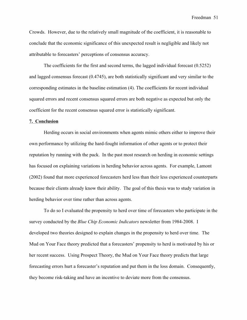
Freedman 51

Crowds. However, due to the relatively small magnitude of the coefficient, it is reasonable to

conclude that the economic significance of this unexpected result is negligible and likely not

attributable to forecasters’ perceptions of consensus accuracy.

The coefficients for the first and second terms, the lagged individual forecast (0.5252)

and lagged consensus forecast (0.4745), are both statistically significant and very similar to the

corresponding estimates in the baseline estimation (4). The coefficients for recent individual

squared errors and recent consensus squared errors are both negative as expected but only the

coefficient for the recent consensus squared error is statistically significant.

7. Conclusion

Herding occurs in social environments when agents mimic others either to improve their

own performance by utilizing the hard-fought information of other agents or to protect their

reputation by running with the pack. In the past most research on herding in economic settings

has focused on explaining variations in herding behavior across agents. For example, Lamont

(2002) found that more experienced forecasters herd less than their less experienced counterparts

because their clients already know their ability. The goal of this thesis was to study variation in

herding behavior over time rather than across agents.

To do so I evaluated the propensity to herd over time of forecasters who participate in the

survey conducted by the Blue Chip Economic Indicators newsletter from 1984-2008. I

developed two theories designed to explain changes in the propensity to herd over time. The

Mud on Your Face theory predicted that a forecasters’ propensity to herd is motivated by his or

her recent success. Using Prospect Theory, the Mud on Your Face theory predicts that large

forecasting errors hurt a forecaster’s reputation and put them in the loss domain. Consequently,

they become risk-taking and have an incentive to deviate more from the consensus.

Freedman 52

Alternatively, during periods of small individual errors, the theory predicts that forecasters

experience risk aversion and a stronger incentive to herd. The Transitory Wisdom of Crowds

theory predicted that herding behavior is driven by the recent accuracy of the consensus forecast.

Specifically, when the consensus forecast is accurate, forecasters are more likely to herd because

they believe the consensus includes valuable private information and is therefore a better target

to herd to, compared to periods of large consensus errors.

The results are quite noteworthy and provide support for both theories. The GNP

forecasting data for both the veterans and the entire sample using the naïve correction for first-

order serial correlation provides strong support for the Theory of the Transitory Wisdom of

Crowds, which predicts that forecasters choose their herding behavior based on the recent

accuracy of the consensus forecast. Additionally, the GNP forecasting data for both the veterans

and the entire sample corrected for complex forms of serial correlation provide strong support for

the Mud on Your Face Theory, which predicts that forecasters choose their herding behavior

based on their recent performance.

Alternatively, the unemployment data provides no support for the Mud on Your Face

Theory and limited support for the Theory of the Transitory Wisdom of Crowds. Specifically,

after correcting the entire samples’ forecasts of unemployment for high order serial correlation,

the results provided support for the Theory of the Transitory Wisdom of Crowds. Conversely,

when only correcting for first-order serial correlation in the entire sample and higher order serial

correlation with the veteran subsample, I found unexpectedly significant results challenging the

Theory of the Transitory Wisdom of Crowds. However, after considering the magnitudes of the

relevant coefficients, I concluded that the unexpected results were likely statistical artifacts and

likely not economically relevant.

Freedman 53

These results provide probative value to consumers of macroeconomic forecasts,

indicating that these consumers should be mindful of the consensus’ and individual forecasters’

recent forecasting accuracy when using their forecasts. Although the results derived from GNP

and unemployment forecasts are useful for considering herding behavior for other variables, the

current results may not be generalizable to other variables. One significant downside to the

application of these results elsewhere is the different types, quality and availability of

information available for other variables. This problem is clear when comparing the results of

the GNP forecasts and the unemployment forecasts; due to the differences between the variables,

such as the release of actual values of the variables on different schedules and with varying

revisions, support for both theories was apparent with the GNP data but neither theory held with

the unemployment data.

Additionally, it would be beneficial to derive more complete theoretical models of

reputation-driven herding that generalize the assumption of risk neutrality made by Scharfstein

and Stein’s (1990) to cases where agents are either risk-averse or risk-taking depending on

whether they are operating in the domain of gains of loses.

Overall, these findings suggest that macroforecasters’ propensity to herd varies over time

and is systematically linked to past performance, both at the individual and group level. These

findings add to the existing literature which has focused almost exclusively on cross-sectional

variation in herding behavior. The finding that herding varies over time and is linked to past

performance suggests that temporal variations in herding could play a role in business cycle

dynamics. In particular, past forecasting success of the consensus could lead to increased

herding which ultimately causes the consensus to poorly aggregate private information and

become a misleading indicator of future economic activity. To the extent that the public relies

Freedman 54

on the consensus to plan and make economic decisions, such inaccuracy could amplify macro

shocks.

Freedman 55

References

Asch, S. E. (1952). Social Psychology. Englewood Cliffs, N.J.: Prentice-Hall.

Bates, J. M., & Granger, C. W. (1969). The combination of forecasts. OR, 20(4), 451-468.

Batchelor, R. A., & Dua, P. (1990). Product differentiation in the economic forecasting industry. International Journal of Forecasting, 6, 311-316.

Bauer, A., Eisenbeis, R. A., Waggoner, D. F., & Zha, T. (2003). Forecast Evaluation with Cross-Sectional Data: The Blue Chip Surveys. Federal Reserve Bank of Atlanta Economic Review, 88(2), 17-32.

Bureau of Labor Statistics. (2012). National Unemployment Rate. Archives available at http://www.bls.gov/cps/cpsaat01.htm.

Bikhchandani, S., Hirshleifer, D., & Welch, I. (1992). A Theory of Fads, Fashion, Custom, and Cultural Change as Informational Cascades. Journal of Political Economy, 100(5), 992-1026.

Bikhchandani, S., Hirshleifer, D., & Welch, I. (1998). Learning from the Behavior of Others: Conformity, Fads, and Informational Cascades. The Journal of Economic Perspectives, 12(3), 151-170.

Camerer, C. F. (1998). Prospect theory in the wild: Evidence from the field. Social Science Working Paper, California Institute of Technology, 1037.

Clemen, R. (1989). Combining forecasts: A review and annotated bibliography. International Journal of Forecasting, 5, 559-583.

Croushore, D., & Stark, T. (2001). A Real-Time Data Set for Macroeconomists. Journal of Econometrics,105, 111-130.

Economic Report of the President. (2012). St. Louis Federal Reserve Bank Economic Library and Archives. Archives available at http://fraser.stlouisfed.org/publication/?pid=45.

Ferderer, J. P., Pandey, B., & Veletsianos, G. (2005). Why do the Blue Chip Forecasters Herd? A Test of Information and Reputation Models. Macalester College.

Gallo, G. M., Granger, C. W. J., & Jeon, Y. (2002). Copycats and common swings: The impact of the use of forecasts in information sets. IMF Staff Papers, 49(1), 4-21.

Galton, F. (1907). Vox populi. Nature, 75, 450-451.

Granger, C. W. J. (1969). Investigating causal relations by econometric models and cross-spectral methods". Econometrica, 37(3), 424–438.

Granger, C. W. J, & Bates, J. M. (1969). The Combination of Forecasts. Operational Research Society, 20(4), 451-468.

Freedman 56

Hong, L. & Page, S.E. (2004). Groups of diverse problem solvers can outperform groups of high-ability problem solvers. Proceedings of National Academy of Sciences, 101, 16385-16389.

Hong, L., Page, S. E., & Riolo, M. (2011). Individual learning and collective intelligence. Draft provided by Scott Page.

Kahneman, D., & Tversky, A. (1979). Prospect theory: An analysis of decision under risk. Econometrica, 47, 263-292.

Kahneman, D., & Tversky, A. (1992). Advances in Prospect Theory: Cumulative representation of uncertainty. Journal of Risk and Uncertainty, 5, 297-323.

Lamont, O. A. (2002). Macroeconomic Forecasts and Microeconomic Forecasters. Journal of Economic Behavior & Organization, 48, 265-280.

Laster, D., Bennett, P. & Geoum, I. S. (1999). Rational bias in macroeconomic forecasts. The Quarterly Journal of Economics, 293-318.

Moore, R. E. (2008). Blue chip economic indicators. Aspen Publishers.

NBER. (2010). US Business Cycle Expansions and Contractions. Public Information Office, National Bureau of Economic Research, Inc. Accessed from: http://www.nber.org/cycles.html

Page, S. (2007). The Difference. Princeton, NJ: Princeton University Press.

Pons-Novell, J. (2004). Behavioural biases among interest rate forecasters. Applied Economics Letters, 11, 319-321.

Scharfstein, D. S. & Stein, J. C. (1990). Herd Behavior and Investment. The American Economic Review, 80(3), 465-479.

Schuh, S. (2001). An Evaluation of Recent Macroeconomic Forecast Errors. New England Economic Review, Jan/Feb, 35-56.

Surowiecki, J. The Wisdom of Crowds. New York, NY: Anchor Books.

Survey of Current Business (2012). Bureau of Economic Analysis. Archives available at http://www.bea.gov/scb/date_guide.asp.

Zarnowitz, V. (1984). The Accuracy of Individual and Group Forecasts from Business Outlook Surveys. Journal of Forecasting, 3(1), 11-26.

Zarnowitz, V. (1992). The Accuracy of Individual and Group Forecasts. In V. Zarnowitz (Eds.), Business Cycles: Theory, History, Indicators, and Forecasting – University of Chicago Press, Chicago, USA.

Freedman 57

Zarnowitz, V. & Braun, P. (1993). Twenty-two Years of the NBER-ASA Quarterly Economic Outlook Surveys: Aspects and Comparisons of Forecasting Performance. In J. Stock & M. Watson (Eds.), Business Cycles, Indicators and Forecasting - University of Chicago Press, Chicago, USA.

Zarnowitz, V., & Lambros, L. A. (1987). Consensus and uncertainty in economic prediction. Journal of Political Economy, 95, 591-621.

Freedman 58

Appendices

Freedman 59

Appendix I: Information About Forecasters in Sample

For a quantitative breakdown of the composition of the forecasters in the sample, see Table II.

Veterans: Bank of America Corp.; Bank One; USA Chamber of Commerce; Chase Manhattan Bank; Conference Board; Chrysler; DuPont; Econoclast; Eggert Economic Enterprises; Evans, Carrol and Associates; Georgia State; University of Maryland Inforum; La Salle National Bank; Macroeconomic Advisors, LLC; Merrill Lynch; Morgan Stanley & Co.; National City Corporation; North Trust Company; Prudential Financial; Prudential Equity Group; SOM Economics Inc.; Turning Point (Micrometrics); U.S. Trust Co.; UCLA Business Forecast; Wayne Hummer & Co. Entire Sample: Industrial Organizations: Caterpillar; USA Chamber of Commerce; Conference Board; Chrysler; Dun & Bradstreet; DuPont; Eaton Corporation; Fannie Mae; Fedex Corp.; Ford Motor Comp.; General Motors Corporation; Metropolitan Insurance; Motorola, Inc.; National Association of Home Builders; National Association of Realtors; Pennzoil Co.; Prudential Financial; Sears Roebuck; Swiss RE; W.R. Grace Co.; Weyerhaueser Co.; Mortgage Banker Association Banks: Bank of America Corp.; Bank One; Bankers Trust; Barnett Banks, Inc.; Brown Brothers Harriman; Chase Manhattan Bank; Chemical Bank; Citicorp Information Services; Comerica; CoreStates Financial Corp.; Credit Suisse; Harris Trust & Savings Bank; Huntington National Bank; Irving Trust Co.; JP Morgan Chase; La Salle National Bank; Marine Midland Bank; National City Corporation; Nations Bank; Northern Trust Co.; Fleet Financial Group; Philadelphia National Bank; PNC Financial Corp.; Security Pacific National Bank; U.S. Trust Co.; Wells Capital Management Securities Firms: Arnhold & S.Bleichroeder; Bear Stearns & Co., Inc.; BMO Capital Markets; C.J. Lawrence, Inc.; Chicago Corporation; CRT Government Securities; Daiwa Research of Institute Americas; Dean Witter Reynolds; Deutsche Banc Alex Brown; Goldman Sachs & Co.; J.W. Coons Advisors; Lehman Brothers; Morgan Guaranty; Morgan Stanley & Co.; Nomura Securities; Prudential Equity Group; Schwab Washington Research Group; UBS; Wachovia Securities; Chicago Capital, Inc.; Mesirow Financials; RBS Greenwich Capital

Econometric Modelers: DRI-WEFA; Fairmodel Economica Inc.; Georgia State; University of Maryland Inforum; Macroeconomic Advisors, LLC; Merrill Lynch; UCLA Business Forecast; University of Michigan M.Q.E.M. Independents: Arthur D. Little; Bostian Research Associates; Business Economics, Inc.; Cahners Publishing Co.; Charles Reeder; Clearview Economics; Econoclast; Econoviews International, Inc.; Eggert Economic Enterprises; Evans, Carrol and Associates; Classicalprinciples.com; Kellner Economic Advisors; MMS International; Moody’s Capital Markets; Morris Cohen & Associates; Naroff Economic Advisors; Peter L. Bernstein, Inc.; Polyconomics; SOM Economics, Inc.; Standard & Poors; Stotler Economics, Inc.; Turning Points (Micrometrics); Wayne Hummer & Co.; Pema Associates; Action Economics; Moody’seconomy.com; Economist Intelligence Unit

Freedman 60

Appendix II: Granger Causality Measures of Herding As additional evidence of herding, Granger Causality tests were used to prove that the

lagged consensus Granger-causes the current period individual forecast, implying that the current

period forecast does not cause the lagged consensus. To complete this analysis, three veterans

were randomly selected from the GNP dataset and the unemployment dataset. All six of these

forecasters provided evidence that the lagged consensus Granger-causes the current period

individual forecast.

According to Granger Causality (Granger, 1969), variable x Granger-cause variable y if:

!!! = !!!!! (1: Restricted)

!!! = !!!!! + !!!!! (2: Unrestricted)

F(2) > F(1), indicating that the lagged value of variable x provides additional explanatory power

to the current period value of y, and if:

!!! = !!!!! (3: Restricted)

!!! = !!!!! + !!!!! (4: Unrestricted)

F(3) = F(4), indicating that the lagged value of variable y does not provides additional

explanatory power to the current period value of x. In the context of the current analysis,

variable y is an individual forecaster’s forecast, and variable x is the consensus forecast.

1. GNP Data

The three forecasters selected from the GNP dataset were Chase Manhattan, Conference

Board, and Chrysler. For Chase Manhattan, the first F-test that the lagged consensus causes the

current period individual forecast, F(1, 189) = 34.82, p < 0.0001, and the second F-test revealed

that the lagged individual forecast does not cause the current period consensus, F(1, 189) = 0.22,

p = 0.6394, revealing that the lagged consensus Granger-causes the current period individual

Freedman 61

forecast. For Conference Board, the first F-test that the lagged consensus causes the current

period individual forecast, F(1, 282) = 8.16, p = 0.0046, and the second F-test revealed that the

lagged individual forecast does not cause the current period consensus, F(1, 282) = 0.16, p =

0.6894, revealing that the lagged consensus Granger-causes the current period individual

forecast. For Chrysler, the first F-test that the lagged consensus causes the current period

individual forecast, F(1, 281) = 22.17, p < 0.0001, and the second F-test revealed that the lagged

individual forecast does not cause the current period consensus, F(1, 281) = 2.31, p = 0.1299,

revealing that the lagged consensus Granger-causes the current period individual forecast.

2. Unemployment Data

The three forecasters selected from the GNP dataset were University of Maryland

Inforum, Northern Trust Company, and Turning Points (Micrometrics). For University of

Maryland Inforum, the first F-test that the lagged consensus causes the current period individual

forecast, F(1, 256) = 59.18, p < 0.0001, and the second F-test revealed that the lagged individual

forecast does not cause the current period consensus, F(1, 256) = 1.54, p = 0.2158, revealing that

the lagged consensus Granger-causes the current period individual forecast. For Northern Trust

Company, the first F-test that the lagged consensus causes the current period individual forecast,

F(1, 269) = 7.56, p = 0.0064, and the second F-test revealed that the lagged individual forecast

does not cause the current period consensus, F(1, 269) = 2.33, p = 0.1279, revealing that the

lagged consensus Granger-causes the current period individual forecast. For Turning Points

(Micrometrics), the first F-test that the lagged consensus causes the current period individual

forecast, F(1, 220) = 30.00, p < 0.0001, and the second F-test revealed that the lagged individual

forecast does not cause the current period consensus, F(1, 220) = 0.86, p = 0.3556, revealing that

the lagged consensus Granger-causes the current period individual forecast.

Freedman 62

Appendix III: Estimation Procedure Rationale

When estimating equations (4) and (5) using panel data, I had to choose to either use a

fixed effects regression or a random effects regression. Theoretically, fixed effects estimation is

more appropriate to the current analysis due to individual variations between the forecasters that

could be accounted for in the individually estimated intercept terms for each forecaster.

However, if fixed effects are not necessary to account for this variance, random effects

estimation is more efficient than fixed effects. To determine the appropriate estimation

procedure, I completed Hausman Tests comparing the estimates of the random effects and fixed

effects estimations of each specification. The Hausman Test compares the coefficient estimates

and variances of the coefficients of the fixed effects and random effects regressions:

(!!" − !!")! (!!" − !!")

where !!" and !!" are the coefficient estimate and variance using fixed effects, respectively and

!!" and !!" are coefficient estimate using random effects, respectively. The differences of the

estimates of the estimates are then compared on a !! distribution:

• !!: Coefficient estimates are consistent between fixed effects and random effects, but

only random effects is efficient

• !!: Coefficient estimates are not consistent between fixed effects and random effects,

only fixed effects is accurate

The results of the Hausman Tests are presented in Table X29. All but one of the Hausman Test

!! statistics are significant, providing grounds for rejecting !! in favor of !! and using fixed

effects estimation. However, after a closer look, it is clear that the estimates between fixed

29 Note: For brevity, Table X only includes Hausman Test results for the models that correct for first order serial correlation. Additional Hausman Tests were conducted for the determined orders of serial correlation for each subsample and yielded similar results.

Freedman 63

effects and random effects are not considerably different. In fact, the average actual difference

between the fixed effect and random effect estimates for all the regressions is .019975. It is

likely that although there are not considerable differences between these estimates, the Hausman

Test statistic was inflated by the sample size of each estimate. Consequently, on further review,

I chose to use random effects estimation to maximize the efficiency of the models.

Freedman 64

Figures and Tables

Freedman 65

Figure 1: Individual value function derived from Prospect Theory

Freedman 66

Figure 2: Forecaster’s perspective during consistent growth

Reputation Gains Domain

Indi

vidu

al U

tility

Current Value

Possible Next Period Outcome if Forecaster Deviates from Consensus

Possible Next Period Outcome ifForecaster Herds to the Consensus

Expected ValueHerding

Expected ValueDeviation

A A'B B'X

X

Freedman 67

Figure 3: Forecaster’s perspective after macroeconomic shock

Reputation Losses Domain

Indi

vidu

al U

tility

Current Value

Expected ValueDeviation

B B'A A'

Possible Next Period Outcome ifForecaster Deviates from Consensus

Possible Next Period Outcome ifForecaster Herds to the Consensus

HerdingExpected Value

X

X

Freedman 68

Figure 4a: Theory of the Transitory Wisdom of Crowds

Figure 4b: Flowchart of The Theory of the Transitory Wisdom of Crowds

Time

Acc

urac

y of

Con

sens

us F

orec

ast

Her

ding

(Wei

ght

on L

agge

d C

onse

nsus

)

t = 2t = 0 t = 1

-Maximum Intragroup Diversity -Maximum Consensus Accuracy

-Decreased Intragroup Diversity -Decreased Consensus Accuracy

Begin Herding

Slowing Herding

Deviating

t = 3 t = 1

t = 2

-Minimum Intragroup Diversity -Minimum Consensus Diversity

Freedman 69

Figure 5: Number of forecasters in subsample (veterans) and total sample.

0

10

20

30

40

50

60

1984 1989 1994 1999 2004 2009

Num

ber of Forecasters in Sample

Year

Veterans

Entire Sample

Freedman 70

Figure 6: Actual GNP/GDP growth vs. forecasting error across time, veterans and entire sample

Figure 7: Actual unemployment vs. forecasting error across time, veterans and entire sample

-‐2

-‐1

0

1

2

3

4

5

6

7

8

1983 1988 1993 1998 2003 2008 Fore casted and Actual rGN

P/rGDP

Grow

th

Year

Veterans Consensus

Entire Sample Consensus

Actual GNP/GDP Growth

3

4

5

6

7

8

9

1983 1988 1993 1998 2003 2008

Forecasted and Actual

Unemployment

Year

Veterans Consensus

Entire Sample Consensus

Actual Unemployment

Freedman 71

Figure 8: Dispersion of veterans’ forecasts of GNP/GDP growth in June

Figure 9: Dispersion of veterans’ forecasts of GNP/GDP growth in December

Freedman 72

Figure 10: Dispersion of all forecasts of GNP/GDP growth in June

Figure 11: Dispersion of all forecasts of GNP/GDP growth in December

Freedman 73

Table I: Summary of predictions of Mud on Your Face Theory (1) and the Theory of the

Transitory Wisdom of Crowds (2). First 2 rows in each box provide the conditions (Accuracy of

individual and consensus); last 2 rows provide the predictions of individual herding behavior

provided by each theory.

Individual: Accurate Individual: Accurate Consensus: Accurate Consensus: Inaccurate Predictions: Predictions: 1: Herd 1: Herd 2: Herd 2: Deviate Individual: Inaccurate Individual: Inaccurate Consensus: Accurate Consensus: Inaccurate Predictions: Predictions: 1: Deviate 1: Deviate 2: Herd 2: Deviate

Table II: Composition of affiliations of forecasters in subsample (veterans) and total sample

across entire sample.

# of Forecasters % # of Forecasters % Industrial Organization 4 16% 19 17%Bank 7 15% 29 14%Securities Firm 2 5% 26 14%Econometric Forecaster 5 14% 8 5%Independent Forecasters 7 22% 31 21%Total 25 100% 120 100%

Veterans Total SampleIndustry Affiliation of Forecasters in Dataset

Freedman 74

Table III: Overview of regression results for all estimations of equation (5).

VariableEntire

Sample

Entire Sample

Corrected

VeteransVeterans

Corrected

Entire Sam

pleEntire Sam

ple C

orrectedVeterans

Veterans C

orrectedLagged Individual Forecast

.7901**0.3448**

0.6407**.4116**

.7174**.3659**

.7082**.5252**

Lagged Consensus Forecast

.2502**.6671**

0.4168**.6447**

.2789**.6083**

.2923**.4745**

Recent Individual Squared Error

0.0002.0729**

0.0206.0661*

-0.00340.0039

-0.1302-0.04

Recent C

onsensus Squared Error.2351**

-.0531*0.2197**

-0.0228 -.9197**

0.5303**-0.0763

-.1964*Lagged Individual A

ccuracy X Lagged C

onsensus-0.002

-.0253**-0.0084

-.0210**0.0003

-0.00180.0161

0.0054Lagged C

onsensus Accuracy X

Lagged Consensus

-0.0755**0.0143

-0.0736**0.0047

.1447** -.0863**

0.0117.0339*

Observations

132812179

59881550

128313192

59344209

Forecasters115

10825

25113

10825

25R

2 Overall

0.94490.9875

0.94560.9858

0.98420.9955

0.98360.9892

Wald C

hi Squared225913.6

171944.84104052.09

107104.53796392.7

708382.39356231.54

384674.54Lags

11,3,6,9,10

11,3,6,8,9

11,2,3,4,6,9

11,2,4

Notes:

1. Dependent variable is the individual current period forecast of rG

NP

2. Coefficient estim

ates reflect average across sample across tim

e using random effects regression

3. Z-statistics (under coefficient estimates): * significant at 5%

, ** significant at 1%4. Lagged values of the dependent variable included to correct for serial correlation (R

eported in last row)

5. Italicized = unexpected, Bold = unexpected and significant

Overview

of Results, R

andom Effects, Equation (5)

rGN

P/rGD

PU

nemploym

ent

Freedman 75

Table IV: Regression results for GNP/GDP data using estimation equations (4) and (5), correcting for first-degree serial correlation.

SpecificationSample Entire Sample Veterans Entire Sample VeteransVariableLagged Individual Forecast 0.7873 0.6413 0.7901 0.6407

149.35** 63.51** 150.21** 64.18**Lagged Consensus Forecast 0.2208 0.374 0.2502 0.4168

40.39** 35.59** 41.13** 36.38**Recent Individual Squared Error 0.0002 0.0206

0.02 0.86Recent Consensus Squared Error 0.2351 0.2197

13.31** 6.75**Recent Individual Squared Error X Lagged Consensus -0.002 -0.0084

-0.56 -0.94Recent Consensus Squared Error X Lagged Consensus -0.0755 -0.0736

-11.48** -6.07**Constant 0.0046 -0.0153 -0.1053 -0.145

0.8 -1.78 -10.58** -9.59**Observations 13788 6214 13281 5988Individuals 115 25 115 25R2 Overall 0.9569 0.9575 0.9449 0.9456Wald Chi Squared 306025.36** 140050.24** 225913.56** 104052.09**Lags 1 1 1 1Notes:1. Dependent variable is the individual current period forecast of rGNP2. Coefficient estimates reflect average across sample across time using random effects regression3. Z-statistics (under coefficient estimates): * significant at 5%, ** significant at 1%4. Lagged values of the dependent variable included to correct for serial correlation (Reported in last row)5. Italicized = unexpected, Bold = unexpected and significant

rGNP/GDP Results, Random Effects GLS, Equations (4) and (5), Correcting for First Degree Serial Correlation(4) (5)

Freedman 76

Table V: Regression results for unemployment data using estimation equations (4) and (5), correcting for first-degree serial correlation.



49.80** 32.70** 46.19** 31.59**Recent Individual Squared Error -0.0034 -0.1302

-0.05 -1.2Recent Consensus Squared Error -0.9197 -0.0763

-5.69** -0.77Recent Individual Squared Error X Lagged Consensus 0.0003 0.0161

0.03 0.92Recent Consensus Squared Error X Lagged Consensus 0.1447 0.0117

5.64** 0.68Constant -0.0336 -0.023 0.0143 -0.0107

-4.95 -2.37* 1.34 -0.75Observations 12831 5934 12831 5934Individuals 113 25 113 25R2 Overall 0.9841 0.9836 0.9842 0.9836Wald Chi Squared 746187.37 356170.03** 796392.67** 356231.54**Lags 1 1 1 1Notes:1. Dependent variable is the individual current period forecast of rGNP2. Coefficient estimates reflect average across sample across time using random effects regression3. Z-statistics (under coefficient estimates): * significant at 5%, ** significant at 1%4. Lagged values of the dependent variable included to correct for serial correlation (Reported in last row)5. Italicized = unexpected, Bold = unexpected and significant

Unemployment Results, Random Effects GLS, Equations (4) and (5), Correcting for First Degree Serial Correlation(4) (5)

Freedman 77

Table VI: Regression results for GNP/GDP data using estimation equations (4) and (5), using serial correlation corrections determined from entire sample.



19.05** 26.79** 39.13** 23.96**Recent Individual Squared Error 0.0729 0.0611

5.44** 2.33*Recent Consensus Squared Error -0.0531 -0.0252

-2.1* -0.67Recent Individual Squared Error X Lagged Consensus -0.0253 -0.0176

-5.48** -1.86Recent Consensus Squared Error X Lagged Consensus 0.0143 -0.0021

1.6 -0.16Constant -0.0270 -0.0560 -0.0280 -0.0245

-3.55** -5.69 -2.13* -1.36Observations 5839 2703 2179 1025Individuals 112 25 108 25R2 Overall 0.9749 0.9812 0.9875 0.9907Wald Chi Squared 226608.20** 141059.26** 171944.84** 107490.07**Lags 1,2,3,7 1,2,3,7 1,3,6,9,10 1,3,6,9,10Notes:1. Dependent variable is the individual current period forecast of rGNP2. Coefficient estimates reflect average across sample across time using random effects regression3. Z-statistics (under coefficient estimates): * significant at 5%, ** significant at 1%4. Lagged values of the dependent variable included to correct for serial correlation (Reported in last row)5. Italicized = unexpected, Bold = unexpected and significant

rGNP/GDP Results, Random Effects GLS, Equations (4) and (5), Using Serial Correlation Corrections Determined from Entire Sample

(4) (5)

Freedman 78

Table VII: Regression results for GNP/GDP data using estimation equations (4) and (5), using serial correlation corrections determined from veterans subsample.



8.59** 23.57** 10.54** 25.14**Recent Individual Squared Error -0.0133 0.0660

-0.087 2.52*Recent Consensus Squared Error 0.0336 -0.0228

1.11 -0.61Recent Individual Squared Error X Lagged Consensus 0.0051 -0.0210

0.96 -2.21*Recent Consensus Squared Error X Lagged Consensus -0.0079 0.0047

-0.74 0.35Constant 0.0042 -0.0141 -0.0556 -0.0958

0.45 -1.39 -3.54** -5.34**Observations 3406 1590 3313 1550Individuals 110 25 109 25R2 Overall 0.9802 0.9890 0.9726 0.9858Wald Chi Squared 22700.3** 141707.68** 117338.99** 107104.53**Lags 1,2,3,6,8,9 1,2,3,6,8,9 1,3,6,8,9 1,3,6,8,9Notes:1. Dependent variable is the individual current period forecast of rGNP2. Coefficient estimates reflect average across sample across time using random effects regression3. Z-statistics (under coefficient estimates): * significant at 5%, ** significant at 1%4. Lagged values of the dependent variable included to correct for serial correlation (Reported in last row)5. Italicized = unexpected, Bold = unexpected and significant

rGNP/GDP Results, Random Effects GLS, Equations (4) and (5), Using Serial Correlation Corrections Determined from Veterans Subsample

(4) (5)

Freedman 79

Table VIII: Regression results for unemployment data using estimation equations (4) and (5), using serial correlation corrections determined from entire sample.



38.05** 26.1** 41.38** 30.87**Recent Individual Squared Error 0.0044 -0.0547

0.06 -0.52Recent Consensus Squared Error 0.5246 -0.0919

3.11** -0.89Recent Individual Squared Error X Lagged Consensus -0.0019 0.0114

-0.18 0.67Recent Consensus Squared Error X Lagged Consensus -0.0852 0.0124

-3.17** 0.69Constant 0.0483 0.0319 0.0199 0.0412

6.78** 3.02** 1.71 2.75**Observations 3285 1549 3191 1500Individuals 108 25 108 25R2 Overall 0.9956 0.9955 0.9955 0.9953Wald Chi Squared 737725.92** 338178.73** 708450.83** 313605.92**Lags 1,4,7,9 1,4,7,9 1,2,3,4,6,9 1,2,3,4,6,9Notes:1. Dependent variable is the individual current period forecast of rGNP2. Coefficient estimates reflect average across sample across time using random effects regression3. Z-statistics (under coefficient estimates): * significant at 5%, ** significant at 1%4. Lagged values of the dependent variable included to correct for serial correlation (Reported in last row)5. Italicized = unexpected, Bold = unexpected and significant

Unemployment Results, Random Effects GLS, Equations (4) and (5), Using Serial Correlation Corrections Determined from Entire Sample

(4) (5)

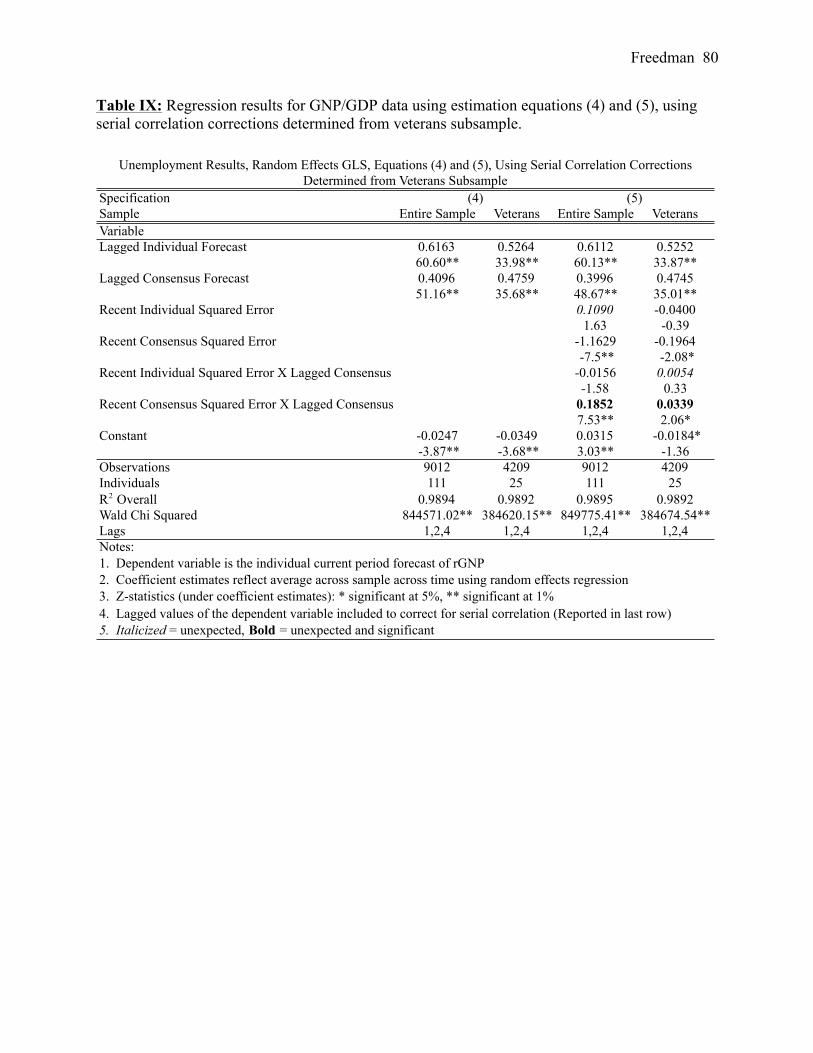
Freedman 80

Table IX: Regression results for GNP/GDP data using estimation equations (4) and (5), using serial correlation corrections determined from veterans subsample.



51.16** 35.68** 48.67** 35.01**Recent Individual Squared Error 0.1090 -0.0400

1.63 -0.39Recent Consensus Squared Error -1.1629 -0.1964

-7.5** -2.08*Recent Individual Squared Error X Lagged Consensus -0.0156 0.0054

-1.58 0.33Recent Consensus Squared Error X Lagged Consensus 0.1852 0.0339

7.53** 2.06*Constant -0.0247 -0.0349 0.0315 -0.0184*

-3.87** -3.68** 3.03** -1.36Observations 9012 4209 9012 4209Individuals 111 25 111 25R2 Overall 0.9894 0.9892 0.9895 0.9892Wald Chi Squared 844571.02** 384620.15** 849775.41** 384674.54**Lags 1,2,4 1,2,4 1,2,4 1,2,4Notes:1. Dependent variable is the individual current period forecast of rGNP2. Coefficient estimates reflect average across sample across time using random effects regression3. Z-statistics (under coefficient estimates): * significant at 5%, ** significant at 1%4. Lagged values of the dependent variable included to correct for serial correlation (Reported in last row)5. Italicized = unexpected, Bold = unexpected and significant

Unemployment Results, Random Effects GLS, Equations (4) and (5), Using Serial Correlation Corrections Determined from Veterans Subsample

(4) (5)

Freedman 81

Table X: Hausman Test Results

Baseline Specification (4) Full Specification (5)Veterans rGNPLagged Individual Forecast -0.0121 -0.0114Lagged Consensus Forecast 0.0121 0.0110Recent Individual Squared Error -0.0197Recent Consensus Squared Error 0.0198Recent Individual Squared Error X Lagged Consensus 0.008Recent Consensus Squared Error X Lagged Consensus -0.0082Number of Observations 6214 5988Chi Squared (Hausman) 21.72** 22.85**Entire Sample rGNPLagged Individual Forecast -0.0076 -0.0082Lagged Consensus Forecast 0.0070 0.0072Recent Individual Squared Error 0.0031Recent Consensus Squared Error -0.0024Recent Individual Squared Error X Lagged Consensus 0.0002Recent Consensus Squared Error X Lagged Consensus 0.0012Number of Observations 13788 13281Chi Squared (Hausman) 17.02** 36.65**Veterans UnemploymentLagged Individual Forecast -0.0047 -0.0049Lagged Consensus Forecast 0.0046 0.0042Recent Individual Squared Error -0.0732Recent Consensus Squared Error -0.0192Recent Individual Squared Error X Lagged Consensus 0.0110Recent Consensus Squared Error X Lagged Consensus 0.0000Number of Observations 5934 5934Chi Squared (Hausman) 6.4* 9.23Entire Sample UnemploymentLagged Individual Forecast -0.0098 -0.0134Lagged Consensus Forecast 0.0103 0.0146Recent Individual Squared Error -0.0798Recent Consensus Squared Error 0.2076Recent Individual Squared Error X Lagged Consensus 0.0124Recent Consensus Squared Error X Lagged Consensus -0.0309Number of Observations 12831 12831Chi Squared (Hausman) 37.62** 69.53**Notes:1. Chi-Squared: * significant at 5%, ** significant at 1%

Actual Difference in Coefficient Estimates Between FE and REHausman Test Results

Documents

Mud on Your Face, Big Disgrace Vs. The Wisdom of Crowds