Embed Size (px)
Citation preview
© Numerical Factory
Numerical Methods in Engineering
Dept. Matemàtiques ETSEIB - UPC BarcelonaTech
Linear Systems
1

© Numerical Factory
Linear Systems: Iterative Methods
11 1 1 1
1 1
n n
m mn n m
a x a x b
a x a x b
+ + = + + =
a Coefficients
x Unknowns
b Independent terms
Linear System
2

© Numerical Factory
Introduction
11 1 1 1
1
n
m mn n n
a a x b
a a x b
=
Ax b=
Matrix Form
3

© Numerical Factory
Matrix Properties
4

© Numerical Factory
MATRIX PROPERTIES
• Matrix Algebra:
– Matrix-Vector product: b=Ax
– Linear Mapping
5

© Numerical Factory
MATRIX PROPERTIES
– Columns
– Alternative view of matrix-vector product
– b is a linear combination of the columns of A
6

© Numerical Factory
MATRIX PROPERTIES
– Matrix- matrix product B=AC
– Matrix-vector product for each column of C
– Transpose of a matrix : changing rows by columns
𝐴𝑇
(𝐴 + 𝐵)𝑇 = 𝐴𝑇 + 𝐵𝑇
(𝐴𝐵)𝑇 = 𝐵𝑇𝐴𝑇
(𝐴𝑇)𝑇 = 𝐴
7
© Numerical Factory
MATRIX PROPERTIES
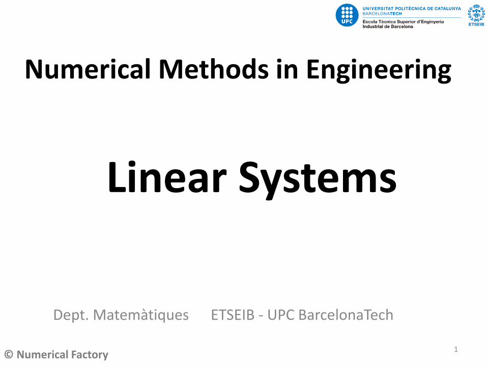
• Determinant:
– 2x2 dim
– Principal minors:
𝑎11 … 𝑎1𝑛⋮ ⋱ ⋮
𝑎𝑚1 ⋯ 𝑎𝑚𝑛
𝑎11 𝑎12𝑎21 𝑎22
= 𝑎11 · 𝑎22−𝑎12 · 𝑎21
Ak
8

© Numerical Factory
MATRIX PROPERTIES
• Det. Properties:
• A is symmetric iff
• Trace: Sum of the diagonal elements
1
n
ii
i
a=
=
det( 𝐴 · 𝐵) = det( 𝐴) · det( 𝐵)
det( 𝐴𝑇) = det( 𝐴)
𝐴𝑇 = 𝐴
9

© Numerical Factory
MATRIX PROPERTIES
• Rank: number of linear independent columns
– Maximum order of the nonvanishing determinant extracted from A.
– A has full rank if rank(A)= min(m,n)
– column rank = row rank
10

© Numerical Factory
MATRIX PROPERTIES
• Rank: number of linear independent columns
– Maximum order of the nonvanishing determinant extracted from A.
– A has full rank if rank(A)= min(m,n)
– column rank = row rank
• Kernel: all solutions of Ax=0
rank + dim(Kernel) = m
11

© Numerical Factory
MATRIX PROPERTIES
• Eigenvalues and Eigenvectors:
– Directions preserved by A
– Deformation induced by A
• Linear homogeneous system:
𝐴𝑣 = λ𝑣
(𝐴 − λ𝐼𝑑)𝑣 = 0
12

© Numerical Factory
MATRIX PROPERTIES
• Inverse of a matrix: (for square matrices)
– If rank(A)=n (or det(A) ≠ 0), A is invertible.
– If A is not invertible is called singular
• A is orthogonal iff
(𝐴 · 𝐵)−1 = 𝐵−1 · 𝐴−1
(𝐴𝑇)−1 = (𝐴−1)𝑇
𝐴𝑇 = 𝐴−1
𝐴 · 𝐴−1 =𝐼𝑑
13

© Numerical Factory
Matrix Types
14

© Numerical Factory
Special Matrices Types
• Diagonal and block diagonal:
– Nonzero entries only at the diagonal
11
mn
a
a
11
mn
A
A
15
© Numerical Factory
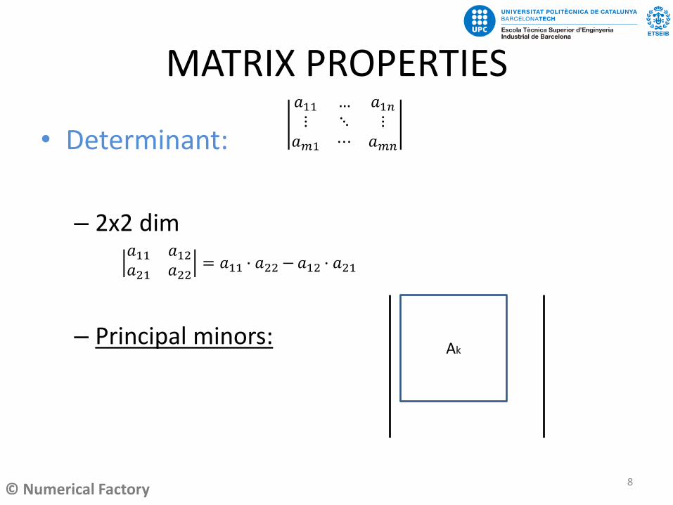
Special Matrices Types
• Triangular Matrices:
– Lower triangular
11
21 22
31 32 33
1 1m mn mn
l
l l
l l l
l l l−
16
© Numerical Factory
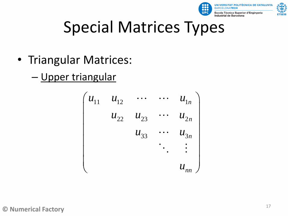
Special Matrices Types
• Triangular Matrices:
– Upper triangular
11 12 1
22 23 2
33 3
n
n
n
nn
u u u
u u u
u u
u
17
© Numerical Factory
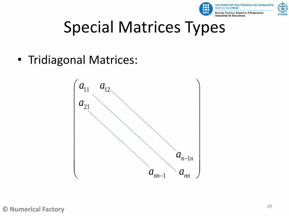
Special Matrices Types
• Tridiagonal Matrices:
11 12
21
1
1
n n
nn nn
a a
a
a
a a
−
−
18

© Numerical Factory
Special Matrices Types
• Hessemberg Matrices:
11 12 1
21
1
1
n
n n
nn nn
a a a
a
a
a a
−
−
19
© Numerical Factory
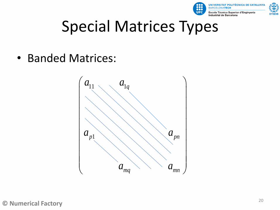
Special Matrices Types
• Banded Matrices:
11 1
1
q
p pn
mq mn
a a
a a
a a
20

© Numerical Factory
Special Matrices Types
• Sparse Matrix
Mainly zero elements
• Special data structures
– Compression
– Efficiency
21

© Numerical Factory
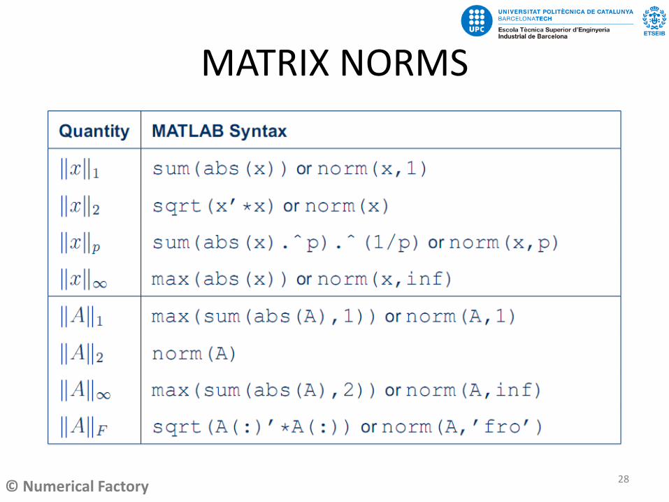
Matrix Norms
22
© Numerical Factory
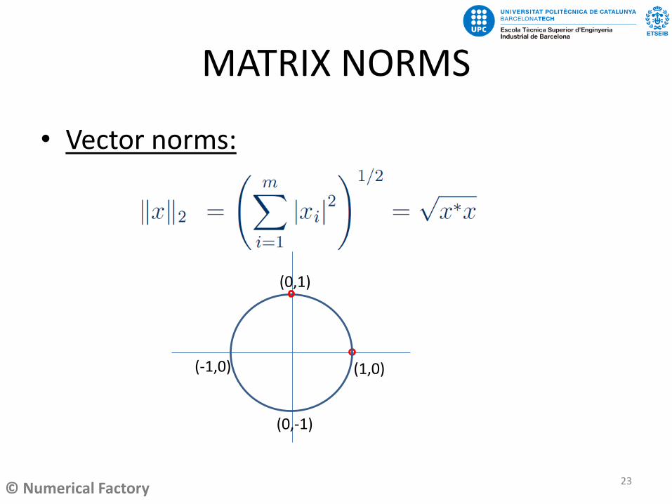
MATRIX NORMS
• Vector norms:
(1,0)(-1,0)
(0,-1)
(0,1)
23

© Numerical Factory
MATRIX NORMS
• Vector norms:
(1,0)(-1,0)
(0,-1)
(0,1)
24

© Numerical Factory
MATRIX NORMS
• Vector norms:
(1,0)(-1,0)
(0,-1)
(0,1)
25

© Numerical Factory
MATRIX NORMS
• Vector norms:
26

© Numerical Factory
MATRIX NORMS
• Induced matrix norms: ∥ 𝐴 ∥𝑘= sup∥ 𝐴𝑥 ∥𝑘∥ 𝑥 ∥𝑘
27
© Numerical Factory
MATRIX NORMS
28

© Numerical Factory
Solving Linear Systems
29

© Numerical Factory
Solving linear systems
• DIRECT METHODS:
– Solution is obtained after a finite number of steps
• Gaussian Elimination, LU, Cholesky, QR, SVD
• ITERATIVE METHODS:
– Solution is obtained as successive approaches
• Jacobi, Gauss-Seidel, Conjugate Gradient
30

© Numerical Factory
Direct Methods
31
© Numerical Factory
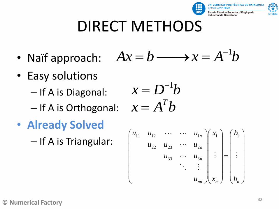
DIRECT METHODS
• Naïf approach:
• Easy solutions
– If A is Diagonal:
– If A is Orthogonal:
• Already Solved
– If A is Triangular:
1Ax b x A b−= ⎯⎯→ =
Tx A b=
1x D b−=
11 12 1 1 1
22 23 2
33 3
n
n
n
nn n n
u u u x b
u u u
u u
u x b
=
32
© Numerical Factory
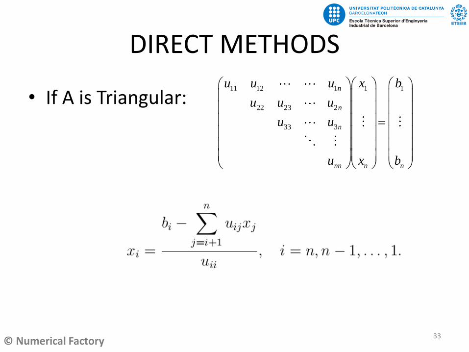
DIRECT METHODS
• If A is Triangular:11 12 1 1 1
22 23 2
33 3
n
n
n
nn n n
u u u x b
u u u
u u
u x b
=
33

© Numerical Factory
DIRECT METHODS
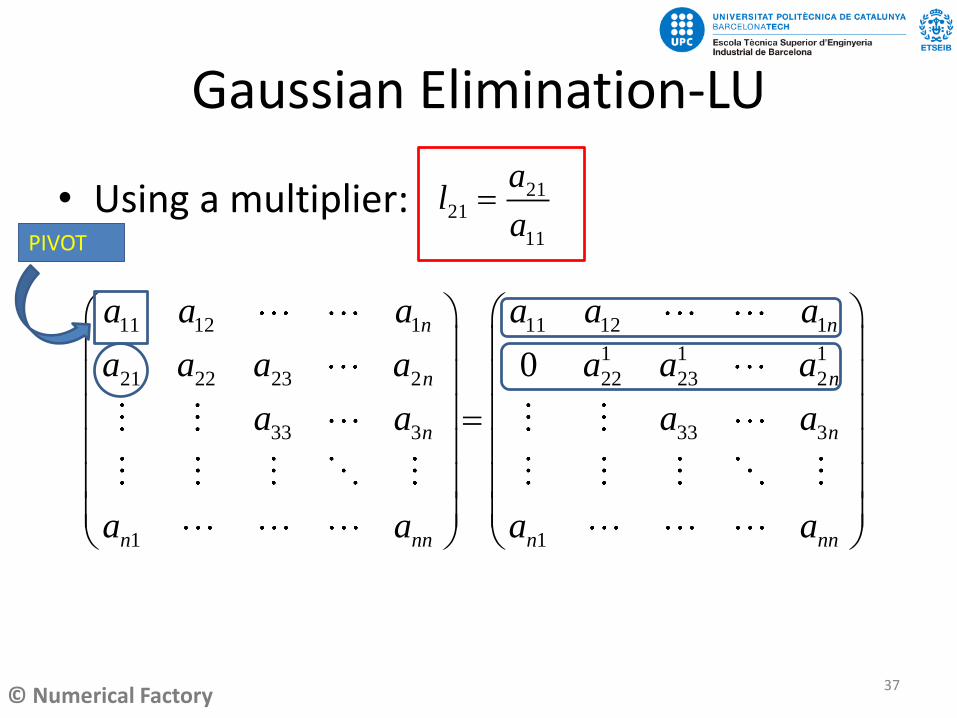
• Gaussian Elimination-LU
– Inverse matrix
– Determinant
• Cholesky
• QR
• SVDAx b=
11 1 1 1
1
n
m mn n n
a a x b
a a x b
=
34

© Numerical Factory
Gaussian Elimination - LU
35

© Numerical Factory
Gaussian Elimination-LU
• Transform the original matrix to an easy form:
11 12 1
22 23 2
33 3
n
n
n
nn
u u u
u u u
u u
u
11 12 1
21 22 23 2
33 3
1
n
n
n
n nn
a a a
a a a a
a a
a a
36
© Numerical Factory
11 12 1 11 12 1
1 1 1
21 22 23 2 22 23 2
33 3 33 3
1 1
0
n n
n n
n n
n nn n nn
a a a a a a
a a a a a a a
a a a a
a a a a
=
Gaussian Elimination-LU
• Using a multiplier: 2121
11
al
a=
PIVOT
37

© Numerical Factory
11 12 1 11 12 1
1 1 1
21 22 23 2 22 23 2
1 1
31 33 3 33 3
1 1
0
0
n n
n n
n n
n nn n nn
a a a a a a
a a a a a a a
a a a a a
a a a a
=
Gaussian Elimination-LU
• Using now multiplier: 31
31
11
al
a=
38

© Numerical Factory
11 12 1 11 12 1
1 1 1
21 22 23 2 22 23 2
1 1
33 3 33 3
1
0
0
0
n n
n n
n n
n nn nn
a a a a a a
a a a a a a a
a a a a
a a a
=
Gaussian Elimination-LU
• Using now multiplier: 11
11
nn
al
a=
39

© Numerical Factory
11 12 1
1 1 1
22 23 2
1 1
33 3
0
0 0
0 0 0 0
n
n
n
nn
a a a
a a a
U a a
a
=
Gaussian Elimination-LU
• Finally:
Upper Triangular
1
11 1
1 1
n
nnnn n
n n
al
a
−
−− −
− −
=
Lower Triangular21
31 32
1 1
1
1
1
1n nn
l
L l l
l l −
=
40

© Numerical Factory
Gaussian Elimination-LU
• System solution from LU decomposition:
• Real Live: Permutations
– Troubles when pivot ≈ 0
·
1.
2.
A LU
Ax b LUx b
Ux y
Ly b
=
= ⎯⎯→ =
=
=
41

© Numerical Factory
Gaussian Elimination-LU
• Row permutations:
11 12 1
1 1 1
22 23 2
1 1
33 3
1
2
0
0
0
n
n
n
k
nn
a a a
a a a
a a
a
a
42

© Numerical Factory
• Row permutations as matrix product
• Finally:
1 2 1
1 0 0 0
0 1
0 0 1
...0
1 0 0 0
0 0 0 0 0 1
k n
ij ij ij ijP P P P P −
= ⎯⎯→ =
Gaussian Elimination-LU
· ·
1.
2.
T
T
P A LU
Ax b LUx P b
Ux y
Ly P b
=
= ⎯⎯→ =
=
=
43

© Numerical Factory
• >> A=rand(6)
• A =
0.8147 0.2785 0.9572 0.7922 0.6787 0.70600.9058 0.5469 0.4854 0.9595 0.7577 0.03180.1270 0.9575 0.8003 0.6557 0.7431 0.27690.9134 0.9649 0.1419 0.0357 0.3922 0.04620.6324 0.1576 0.4218 0.8491 0.6555 0.09710.0975 0.9706 0.9157 0.9340 0.1712 0.8235
• >> [L,U,P]=lu(A)
L =
1.0000 0 0 0 0 00.1068 1.0000 0 0 0 00.8920 -0.6711 1.0000 0 0 00.9917 -0.4726 0.5368 1.0000 0 00.1390 0.9491 -0.0517 -0.2586 1.0000 00.6923 -0.5883 0.5947 0.8836 0.0470 1.0000
MATLAB-LU
U =
0.9134 0.9649 0.1419 0.0357 0.3922 0.04620 0.8676 0.9006 0.9302 0.1293 0.81850 0 1.4349 1.3846 0.4156 1.21410 0 0 0.6204 0.2068 -0.27890 0 0 0 0.6408 -0.51570 0 0 0 0 0.0953
P =
0 0 0 1 0 00 0 0 0 0 11 0 0 0 0 00 1 0 0 0 00 0 1 0 0 00 0 0 0 1 0
44

© Numerical Factory
MATLAB-LU
b =
123456
>> y=L\P*b;
x=U\y;
A*x-b
ans =
1.0e-014 *
-0.7105
-0.7772
0
0
0.3553
0.7105
45

© Numerical Factory
LU applications
46

© Numerical Factory
Application: Inverse of a Matrix
• Inverse as n-linear systems:
11 12 1 11 12 1
21 22 23 2 21 22 23 2
33 3 33 3
1 1
1 0 0
0 1 0 0
0 1
0
0 0 1
n n
n n
n n
n nn n nn
a a a x x x
a a a a x x x x
a a x x
a a x x
=
A 1A− Id
47

© Numerical Factory
Application: Inverse of a Matrix
• Inverse as n-linear systems:
11 12 1 11 12 1
21 22 23 2 21 22 23 2
33 3 33 3
1 1
1 0 0
0 1 0 0
0 1
0
0 0 1
n n
n n
n n
n nn n nn
a a a x x x
a a a a x x x x
a a x x
a a x x
=
A 1A− Id
48

© Numerical Factory
Application: Inverse of a Matrix
• The cost is NOT n times a linear system:
– LU decomposition ONLY ONCE!!
– n times: solution of two triangular systems
iLy e
Ux y
=
=
·A LU=
0
1
0
iwhere e
=
49

© Numerical Factory
Application: Determinant of a Matrix
• Determinant from LU decomposition:
11 12 1 11 12 1
21 22 23 2 21 22 23 2
33 3 31 32 33 3
1 1 1
1
1 0
1 · 0
0
1 0 0
n n
n n
n n
n nn n nn nn
a a a u u u
a a a a l u u u
a a l l u u
a a l l u−
=
50

© Numerical Factory
Application: Determinant of a Matrix
• Determinant from LU decomposition:
From prop. det(AB) = det(A) · det(B)
11 12 1 11 12 1
21 22 23 2 21 22 23 2
33 3 31 32 33 3
1 1 1
1
1 0
1 · 0
0
1 0 0
n n
n n
n n
n nn n nn nn
a a a u u u
a a a a l u u u
a a l l u u
a a l l u−
=
51
det( 𝐴) = det( 𝐿) · det( 𝑈)/ det( 𝑃) = (−1)𝑝ෑ
1
𝑛
𝑢𝑖𝑖
𝑃 ∗ 𝐴 = 𝐿 ∗ 𝑈

© Numerical Factory
Cholesky
52

© Numerical Factory
• If A is a symmetric positive definite matrix
(i)
(ii)
(all principal minors >= 0)
• LU can be obtained without pivoting :
• Cost
LU: Cholesky Decomposition
0Tx Ax
TA A= A2
A3
·TA R R=
53
A4
>> R = chol(A)
© Numerical Factory
QR - decomposition
54

© Numerical Factory
Matrix Decomposition-QR
• Appropriate for non-square systems (overdetermined systems)
·
=
A Q
mxn mxm mxn
R
55

© Numerical Factory
QR Decomposition
• Matrix A as a product of an Orthogonal matrix and an upper triangular one.
11 12 1 11 12 1 11 12 1
21 22 23 2 21 22 23 2 22 23 2
33 3 33 3 33 3
1 1
0
· 0
0
0 0
n n n
n n n
n n n
n nn n nn nn
a a a q q q r r r
a a a a q q q q r r r
a a q q r r
a a q q r
=
1TQ Q−= R
56

© Numerical Factory
Matrix Decomposition-QR
• Solution “only” a triangular system
·
T
A Q R
Ax b QRx b
Rx Q b
=
= ⎯⎯→ =
=
57
© Numerical Factory
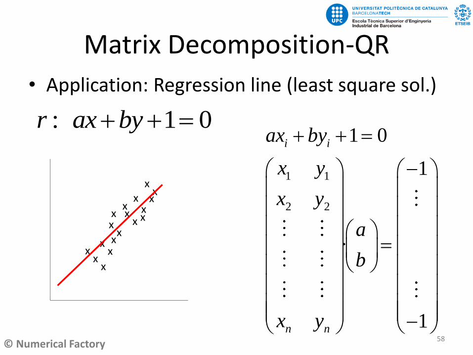
Matrix Decomposition-QR
• Application: Regression line (least square sol.)
: 1 0r ax by+ + =
x xxx
xx
xx
xx xx
xx
xx
xx
1 1
2 2
1 0
1
·
1
i i
n n
ax by
x y
x y
a
b
x y
+ + =
−
=
−
58

© Numerical Factory
SVD - decomposition
59

© Numerical Factory
· .
=
Singular Value Decomposition-SVD
• , with U, V orthogonals and D diagonal
A U v
TA UDV=
mxn mxm mxn nxn
D
60

© Numerical Factory
Singular Value Decomposition-SVD
• Solution from SVD:
• >>svd
1
1
T
T
T T
T T
T
A UDV
Ax b UDV x b
DV x U b
V x D U b
x VD U b
−
−
=
= ⎯⎯→ =
=
=
=
61

© Numerical Factory
Singular Value Decomposition-SVD
• Singular values:
• rank(A) is the number of σi ≠ 0
• Norm
• Decomposition
1 2( , ,......., )nD diag=
1 2 ...... n
1 =
( ) ( ) ( )1 1 1 2 2 2· · ..... ·T T T
n n nu v u v u v
= + + +
·n
T
i i i
i
u v=
=
62

© Numerical Factory
Singular Value Decomposition-SVD
• Singular values:
• rank(A) is the number of σi ≠ 0
• Norm
• Decomposition
1 2( , ,......., )nD diag=
1 2 ...... n
1 =
( ) ( ) ( )1 1 1 2 2 2· · ..... ·T T T
n n nu v u v u v
= + + +
·n
T
i i i
i
u v=
=
63nxn matrix nxn matrix nxn matrix

© Numerical Factory
Singular Value Decomposition-SVD
• Low rank approximation:
• Compression: kx(m+n) instead of mxn
·k
T
i i i
i
u v
=
= 1k + − =
64
© Numerical Factory
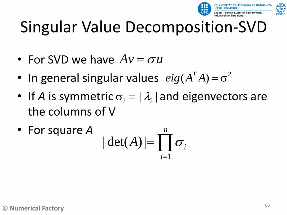
Singular Value Decomposition-SVD
• For SVD we have
• In general singular values
• If A is symmetric and eigenvectors are the columns of V
• For square A
| |i i =
2( )Teig A A =
Av u=
1
| det( ) |n
i
i
A =
=
65

© Numerical Factory
Singular Value Decomposition-SVD
• Stability:
• Condition number:
– Better if
– In general
– Using Norm2
– >> Hilbert Matrix
1
n
=
|| || / || ||sup
|| || / || ||
x x
A A
=
)x x b b ( + )( + = +
· ||−
66

© Numerical Factory
MATLAB-LU
67

© Numerical Factory
Iterative Methods
68

© Numerical Factory
ITERATIVE METHODS
• Compute successive approximations of the solution that “hopefully”converges to the real solution
• Appropriate for large systems (n>1000)
• Faster than direct methods
• Less memory requirements
• Handle special structures (sparse matrices)
(1) (2) ( ), ,....., nx x x
69

© Numerical Factory
ITERATIVE METHODS
• Stationary Methods: Finds a splitting of the matrix , with M invertible
and iterate
converges iff
– Jacobi, Gauss-Seidel, Successive Overrelaxation (SOR)
A M K= +
( 1) 1 ( ) ( )
( )
( )k k k
Ax b
M K x b
Mx Kx b
x M Kx b Rx c+ −
=
+ =
= − +
= − + = +
( 1)kx + ( ) 1R
70

© Numerical Factory
ITERATIVE METHODS
• Krylov subspace methods: use only multiplication by A (or A ) and find solutions in the Krylov subspace generated by
– Conjugate Gradient (CG)
– Generalized Minimal Residual (GMRES)
2 3 1, , , ,....., kb Ab A b A b A b−
T
71

© Numerical Factory
STATIONARY METHODS
• Jacobi Method:
– Idea: to solve ith-unknown for the ith-equation
1 2 3
1 2 3
1 2 3
10 12
10 12
10 12
x x x
x x x
x x x
+ + =
+ + = + + =
( 1) ( ) ( )
1 2 3
( 1) ( ) ( )
2 1 3
( 1) ( ) ( )
3 1 2
1( 12)
10
1( 12)
10
1( 12)
10
k k k
k k k
k k k
x x x
x x x
x x x
+
+
+
= − − +
= − − +
= − − +
72

© Numerical Factory
STATIONARY METHODS
• Jacobi: Split the original matrix11 12 1 11 12 1
21 22 23 2 21 22 23 2
33 3 31 32 3
1 1 1
0 0 0 0
0 0 0 0
0 0 0
0 0
0 0 0 0
n n
n n
n n
n nn n nn nn
a a a a a a
a a a a a a a a
a a a a a
a a a a a−
= + +
( 1) 1 ( )
1 ( )
,
( )
( ( ) )
L D U
D L U
k k
k
D L U
A A A A
M A K A A
x M Kx b
A A A x b
+ −
−
= + +
= = +
= − + =
= − + +
A M K= +
73

© Numerical Factory
STATIONARY METHODS
• Jacobi : Split the original matrix
>>AL=tril(A,-1)
>>AU=triu(A,1)
>>AD=diag(diag(A))
>>Xkp1=inv(AD)*(-(AL+AU)*Xk+b)
11 12 1 11 12 1
21 22 23 2 21 22 23 2
33 3 31 32 3
1 1 1
0 0 0 0
0 0 0 0
0 0 0
0 0
0 0 0 0
n n
n n
n n
n nn n nn nn
a a a a a a
a a a a a a a a
a a a a a
a a a a a−
= + +
A M K= +
74
© Numerical Factory
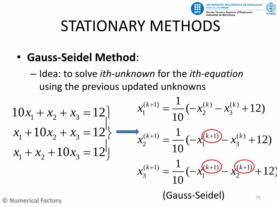
STATIONARY METHODS
• Gauss-Seidel Method:
– Idea: to solve ith-unknown for the ith-equation using the previous updated unknowns
1 2 3
1 2 3
1 2 3
10 12
10 12
10 12
x x x
x x x
x x x
+ + =
+ + = + + =
( 1) ( ) ( )
1 2 3
( 1) ( 1) ( )
2 1 3
( 1) ( 1) ( 1)
3 1 2
1( 12)
10
1( 12)
10
1( 12)
10
k k k
k k k
k k k
x x x
x x x
x x x
+
+ +
+ + +
= − − +
= − − +
= − − +
75(Gauss-Seidel)

© Numerical Factory
STATIONARY METHODS
• Gauss-Seidel: Split the original matrix11 12 1 11 12 1
21 22 23 2 21 22 23 2
33 3 31 32 3
1 1 1
0 0 0
0 0 0
0 0
0 0
0 0 0
n n
n n
n n
n nn n nn nn
a a a a a a
a a a a a a a a
a a a a a
a a a a a−
= +
( 1) 1 ( )
1 ( )
,
( )
( )
LD U
LD U
k k
k
LD U
A A A
M A K A
x M Kx b
A A x b
+ −
−
= +
= =
= − + =
= − +76

© Numerical Factory
STATIONARY METHODS
• Gauss-Seidel: Split the original matrix
>>AL=tril(A,-1)
>>AU=triu(A,1)
>>AD=diag(diag(A))
>>Xkp1=inv(AD+AL)*(-AU*Xk+b)
11 12 1 11 12 1
21 22 23 2 21 22 23 2
33 3 31 32 3
1 1 1
0 0 0
0 0 0
0 0
0 0
0 0 0
n n
n n
n n
n nn n nn nn
a a a a a a
a a a a a a a a
a a a a a
a a a a a−
= +
77

© Numerical Factory
STATIONARY METHODS
• Successive Overrelaxation Method (SOR): The Gauss-Seidel step is extrapolated by a factor
where is the Gauss-Seidel iterate.
• If Gauss-Seidel
• If Overrelaxation
• If Underrelaxation.
=
78

© Numerical Factory
STATIONARY METHODS
• Convergence:– If A is strictly row diagonal dominant
Jacobi and G-S converges.
– If A is symmetric positive definite G-S and SOR converges for
– In general is hard to choose, if the spectral radius of the Jacobi iteration matrix then the optimal is
– G-S can be twice as fast as Jacobi
| | | |ii ij
i j
a a
( )JR
2
1 1 ( )JR =
+ −
79

© Numerical Factory
Conjugate Gradient
80

© Numerical Factory
CONJUGATE GRADIENTS METHOD
• Optimization Problem:
– Solving the system is equivalent to
minimize the quadratic function:1
2
( ) T Tx x Ax x b = −
0Ax b− =
81

© Numerical Factory
CONJUGATE GRADIENTS METHOD
• Optimization Problem:
– The minimization can be done by line searches where is minimized along search direction ( )nx
np
82

© Numerical Factory
CONJUGATE GRADIENTS METHOD
– The that minimizes
is with residual
– The residual is also the Gradient of
– Simple approach: set the search direction to the negative gradient
1( )n n nx p ++
1
T
n nn T
n n
p r
p Ap + = n nr b Ax= −
1n +
( )nx
'( )n n nx Ax b r = − = −
np
nr83
1
2
( ) T Tx x Ax x b = −

© Numerical Factory
CONJUGATE GRADIENTS METHOD
The optimization procedure can be improved by better search directions:
Let the search directions be A-conjugate:
Then the algorithm converges in at most n steps.
0T
i kp Ap =
84

© Numerical Factory
CONJUGATE GRADIENTS METHOD
85
Only few storage vectors needed
Finds the best solution in norm

© Numerical Factory
PRECONDITIONING
• The idea is to modify the initial system using a non-singular preconditioner matrix
• Convergence properties based on
• Trade-off between the cost of applying and the improvement of the convergence properties.
• Very usual:
Ax b=
1 1M Ax M b− −=1M A−
1M −
( )M diag A=
86

© Numerical Factory
PRECONDITIONING
87
𝐩0 ≔ 𝑀−1𝐫0𝐳0: = 𝐩0
𝐳𝑘+1 = 𝑀−1𝐫𝑘+1
𝛽𝑘 ≔𝐫𝑘+1𝑇 𝐳𝑘+1
𝐫𝑘𝑇𝐫𝑘
𝐩𝑘+1 ≔ 𝐳𝑘+1 + 𝛽𝑘𝐩𝑘
Just change these few lines

© Numerical Factory
CG code and Examples
88
function x = conjgrad (A, b, x, tol)
r = b - A * x;
p = r;
rsold = r' * r;
for i = 1:length(b)
Ap = A * p;
alpha = rsold / (p' * Ap);
x = x + alpha * p;
r = r - alpha * Ap;
rsnew = r' * r;
if sqrt(rsnew) < tol
break
end
beta=rsNew / rsOld;
p = r + beta * p;
rsold = rsnew;
end
end

© Numerical Factory
CG code and Examples
89
Simple test example:
A = [5,-2,0;
-2, 5,1;
0, 1,5];
b = [20; 10; -10];
tol = 1.e-10;
x0 = zeros(size(A,2),1);
x = conjgrad (A, b, x0, tol)
© Numerical Factory
CG code and Examples
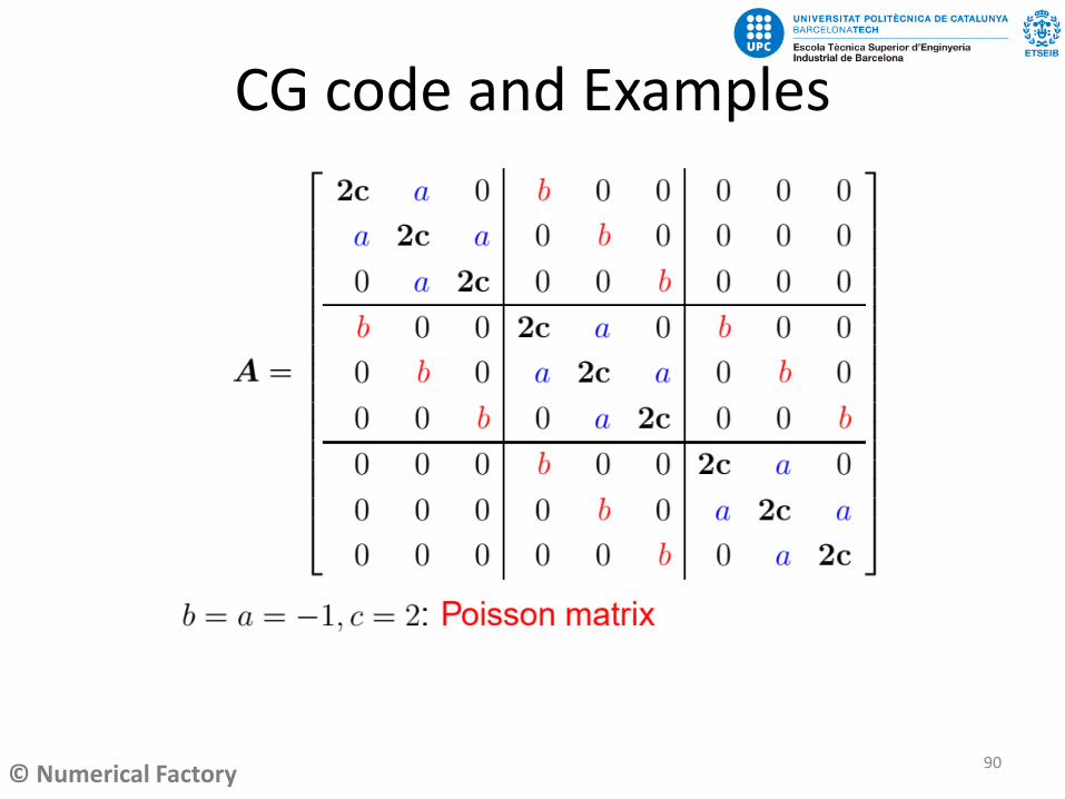
90

© Numerical Factory
Block Tridiagonal Matrix
91
Poisson matrix
𝐴𝑥 = 𝑏 with 𝑏 = ℎ2𝑓(𝑥𝑖 , 𝑦𝑖)where (𝑥𝑖 , 𝑦𝑖) are the nodes in the rectangular division NxN