Embed Size (px)
Citation preview

i
Evaluation of Land Use Scenarios using a Travel Demand
Model for Mumbai Metropolitan Region
M.Tech Dissertation
Submitted in partial fulfillment of the requirements for the degree of
Master of Technology
Submitted by
Srinivas G
(Roll No. 09304020)
Under the supervision of
Prof. K. V. Krishna Rao
Transportation Systems Engineering
Department of Civil Engineering
Indian Institute of Technology Bombay
May, 2011
Evalua
tion o
f Lan
d Use
Sce
nario
s usin
g a Trav
el Dem
and M
odel
for M
umba
i Metr
opoli
tan R
egion
, Srin
ivas G
, IIT B
omba
y

Evalua
tion o
f Lan
d Use
Sce
nario
s usin
g a Trav
el Dem
and M
odel
for M
umba
i Metr
opoli
tan R
egion
, Srin
ivas G
, IIT B
omba
y

iii
DECLARATION
I declare that this written submission represents my ideas in my own words and where others
ideas or words have been included; I have adequately cited and referenced the original
sources. I also declare that I have adhered to all principles of academic honesty and integrity
and have not misrepresented or fabricated or falsified any idea/data/fact/source in my
submission. I understand that any violation of the above will be cause for disciplinary action
by the Institute and can also evoke penal action from the sources which have thus not been
properly cited or from whom proper permission has not been taken when needed.
_________________________________
(Signature)
Srinivas G
________________________________
(Name of the student)
09304020
_________________________________
(Roll No.)
Date: __________
Evalua
tion o
f Lan
d Use
Sce
nario
s usin
g a Trav
el Dem
and M
odel
for M
umba
i Metr
opoli
tan R
egion
, Srin
ivas G
, IIT B
omba
y

iv
INDIAN INSTITUTE OF TECHNOLOGY-BOMBAY, INDIA
CERTIFICATE OF COURSE WORK
This is to certify that Srinivas G (Roll No: 09304020) was admitted to the candidacy of the
M.Tech Degree on 25th
May, 2011, after successfully completing all the courses required for
the M.Tech Degree Programme. The details of the course done are given below:
Sl. No. Course No. Course Name
Credits
1. CE-605 Applied Statistics 6.0
2. IE-601 Optimization Techniques 8.0
3. CE-740 Traffic Engineering 8.0
4. CE-751 Urban Transportation Systems Planning 8.0
5. CE-753 Traffic Design and Studio 4.0
6. CE-694 Credit Seminar 4.0
7. CE-742 Pavement Systems Engineering 8.0
8. CE-780 Behavioral Travel Modelling 6.0
9. CE-754 Economic Evaluation and Analysis of
Transportation Projects 6.0
10. HS-699 Communication and Presentation Skills 4.0
11. HS-618 Introduction to Indian Astronomy 6.0
12. CE-609 Transportation Infrastructures Systems 6.0
I.I.T. Bombay
Dated: Dy. Registrar (Academic)
Evalua
tion o
f Lan
d Use
Sce
nario
s usin
g a Trav
el Dem
and M
odel
for M
umba
i Metr
opoli
tan R
egion
, Srin
ivas G
, IIT B
omba
y

v
Abstract
Mumbai has been experiencing continuous growth and change. The total number of trips is
drastically increasing due to heavy growth in population and employment. The current bus
transit system and sub-urban railway network in Mumbai Metropolitan Region (MMR) is
already overloaded in Mumbai. In congested localities the average speed of buses are as low
as 6 KMPH. With increase in private vehicle (PV) ownership (both cars and two wheelers)
the situation is going to be much worse unless the existing public transportation network is
augmented by modern transit facilities like the Metro Rail, Mono Rail and BRTS, etc. Hence
the MMRDA proposed the different public transport systems which will be completed by the
horizon year 2031. In the developing countries like India the land use planning cannot be
done by integrating it with transportation systems accessibility. Hence it is not practicable to
evaluate the proposed transportation system w.r.t. different land use scenarios using integrated
land use transport models. Hence the sixteen possible land use scenarios were developed by
MMRDA exogenously, which are evaluated w.r.t. proposed transportation system
performance perspective.
The aim of the present study is to evaluate land use scenarios with respect to proposed
transportation system for the horizon year 2031 using a travel demand model. To achieve the
aim, the travel demand model is to be developed for entire MMR by considering the all the
transportation systems which are proposed. Towards the travel demand modeling the region
has been divided into 1037 total number of zones. Then highway network has been developed
using ArcGIS, TransCAD and CUBE Voyager. The public transportation system routes are
coded in GIS based CUBE Voyager software (Script based travel demand modeling software)
for all the transport service options. Then the four steps of travel demand modeling are
implemented using the in the CUBE Voyager software. The set of possible and quantifiable
indicators are selected for the evaluation of urban transportation system performance and they
are assigned with relative scores through a rating survey. The working model is used to test
the different land use scenarios with respect to the selected indicators in a Multi Criteria
Decision Making (MCDM) technique to come up with the best scenario.
Key Words: MMR, travel demand model, CUBE Voyager, land use scenarios, evaluation,
transportation system, MCDM
Evalua
tion o
f Lan
d Use
Sce
nario
s usin
g a Trav
el Dem
and M
odel
for M
umba
i Metr
opoli
tan R
egion
, Srin
ivas G
, IIT B
omba
y

vi
Table of Contents
DISSERTATION APPROVAL SHEET ............................................................................ ii
DECLARATION ............................................................................................................... iii
Abstract ............................................................................................................................... v
Table of Contents ............................................................................................................... vi
List of Figures .................................................................................................................... ix
List of Tables ...................................................................................................................... xi
Chapter 1 ............................................................................................................................. 1
Introduction ........................................................................................................................ 1
1.1 General ...........................................................................................................................................1
1.2 Problem statement ..........................................................................................................................1
1.3 Objectives and Scope of the Study .................................................................................................2
1.4 Organization of the Report .............................................................................................................3
Chapter 2 ............................................................................................................................. 5
Literature Review ............................................................................................................... 5
2.1 General ...........................................................................................................................................5
2.2 Metropolitan Regional Travel Demand Modeling .........................................................................5
2.2.1 Baltimore Regional Travel Demand Model ............................................................................5
2.2.2 San Francisco Metropolitan area Travel Demand Model ........................................................7
2.3 GIS in Travel Demand Modeling ...................................................................................................8
2.4 Land use and Transport Interaction ................................................................................................9
2.4.1 Structure of Land use Transportation Interaction Models .....................................................11
2.4.2 Uncertainty in Integrated Land use Transport Models ..........................................................13
2.5 Evaluation indicators for the land use scenarios ..........................................................................15
2.5.1 Guide lines for selecting the indicators .................................................................................16
2.5.2 Multiple Criteria Decision Making in Transportation Planning ............................................21
2.5.3 Inferences from the literature ................................................................................................22
2.6 Summary .....................................................................................................................................22
Chapter 3 ........................................................................................................................... 23
Study Area and Planning Variables ................................................................................. 23
3.1 General .........................................................................................................................................23
3.2 Study Area ....................................................................................................................................23
3.3 Zoning System .............................................................................................................................24
3.4 Planning Variables .......................................................................................................................25
3.4.1 Road Network and Transport System ...................................................................................28
Evalua
tion o
f Lan
d Use
Sce
nario
s usin
g a Trav
el Dem
and M
odel
for M
umba
i Metr
opoli
tan R
egion
, Srin
ivas G
, IIT B
omba
y

vii
3.4.2 Alternate Growth Scenarios ..................................................................................................28
3.5 Summary ......................................................................................................................................29
Chapter 4 ........................................................................................................................... 30
Methodology ...................................................................................................................... 30
4.1 General .........................................................................................................................................30
4.2 Development of highway and public transit network ..................................................................30
4.2.1 Highway network development.............................................................................................30
4.2.2 Public Transport Network Development ...............................................................................31
4.3 Updating Base year Travel pattern from the previous study ........................................................31
4.4 Horizon year Travel Demand Forecasts .......................................................................................33
4.5 Development of indices for the evaluation of different growth scenarios ...................................33
4.6 Evaluation of Land use Scenarios using Travel Demand Model .................................................34
4.6.1 Formulation of MCDM approach for evaluation ..................................................................35
4.7 Summary ......................................................................................................................................37
Chapter 5 ........................................................................................................................... 39
Travel Demand Model Development................................................................................ 39
5.1 General .........................................................................................................................................39
5.2 Updating Base year Travel pattern from the previous study ........................................................39
5.3 Network Development .................................................................................................................39
5.3.1 Highway Network Development ...........................................................................................39
5.3.2 Available Data Set .................................................................................................................40
5.3.3 Creation of GIS Database ......................................................................................................41
5.3.4 Building the Highway Network ............................................................................................42
5.4 Public Transport Network Development ......................................................................................44
5.4.1 Bus Network ..........................................................................................................................45
5.4.2 Sub urban Rail Network ........................................................................................................46
5.4.3 Metro Rail Network ..............................................................................................................47
5.4.4 Mono Rail Network ...............................................................................................................48
5.4.5 BRT (Bus Rapid Transit) Network .......................................................................................48
5.4.6 Fare Tables and Wait curves .................................................................................................48
5.4.7 Creation of Access/Egress and Transfer links .......................................................................49
5.5 Generation of Initial Highway and Public Transport Skims ........................................................50
5.6 Trip Generation ............................................................................................................................51
5.7 Trip Distribution Models ..............................................................................................................54
5.8 Modal Split Models ......................................................................................................................55
5.9 Highway and Public Transport Assignment .................................................................................57
5.9.1 Public Transport Assignment ................................................................................................57
Evalua
tion o
f Lan
d Use
Sce
nario
s usin
g a Trav
el Dem
and M
odel
for M
umba
i Metr
opoli
tan R
egion
, Srin
ivas G
, IIT B
omba
y

viii
5.9.2 Highway Assignment ............................................................................................................58
5.10 Salient features of the present model .........................................................................................59
5.11 Summary ....................................................................................................................................60
Chapter 6 ........................................................................................................................... 61
Evaluation of Urban Transportation System’s Performance using MCDM approach . 61
6.1 General .........................................................................................................................................61
6.2 Selected Scenarios ........................................................................................................................61
6.3 Calculation of Selected indicators from the Travel Demand Model ............................................62
6.3.1 Accessibility to the public transport stops .............................................................................62
6.3.2 Total Public transport user cost in generalized time units .....................................................63
6.3.3 Traffic Congestion .................................................................................................................64
6.3.4 Transportation safety .............................................................................................................65
6.3. 5 Mode share of the public transport .......................................................................................65
6.3.6 Average trip length and vehicle kilometers ...........................................................................69
6.3.7 Cost of the proposed transportation infrastructure for the Horizon year 2031 ......................70
6.4 Analysis of the Rating survey ......................................................................................................70
6.4.1 Inferences from survey ..........................................................................................................71
6.4.2 Calculation of Relative Transportation performance Index ..................................................72
Chapter 7 ........................................................................................................................... 75
Summary and Conclusions ............................................................................................... 75
7.1 Summary of work .........................................................................................................................75
7.2 Conclusions ..................................................................................................................................76
7.3 Limitations ...................................................................................................................................77
7.4 Future Scope of the work .............................................................................................................78
References ......................................................................................................................... 79
Acknowledgments ............................................................................................................. 81
Appendix ........................................................................................................................... 82
Evalua
tion o
f Lan
d Use
Sce
nario
s usin
g a Trav
el Dem
and M
odel
for M
umba
i Metr
opoli
tan R
egion
, Srin
ivas G
, IIT B
omba
y

ix
List of Figures
Figure No. Description Page No.
Figure 2.1 The Summary of Baltimore Regional Travel demand Model 6
Figure 2.2 Summary of San Francisco Travel demand model 8
Figure 2.3 Architecture of GIS based decision supportive system 9
Figure 2.4 Land use transportation feedback cycle 10
Figure 2.5 The general structure of integrated land use and transport model 12
Figure 2.6 Typical impacts over time of uncertainty in population and employment
(exogenous production) forecasts on model outputs 14
Figure 2.7 Typical impacts over time of uncertainty in commercial trip generation
rates on model outputs 15
Figure 2.8 The role of indicators in a transportation planning process 20
Figure 2.9 sustainability indicator prism 20
Figure 3.1 Sub Regions of MMR 24
Figure 3.2 Forecasted Population of MMR from 1971 to 2031 26
Figure 4.1 Methodology for updating base year travel pattern 32
Figure 4.2 Formulation of procedure for Evaluation of land use scenarios w.r.t.
transportation system performance 35
Figure 4.3 Methodology for Evaluation of Land use scenarios for the horizon years
using Travel Demand Model 38
Figure 5.1 Local and arterials links 41
Figure 5.2 freeway links 41
Figure 5.3 suburban rail 41
Figure 5.4 The geo referenced shape file of total MMR network developed in
TransCAD 42
Figure 5.5 Process for the development of network for MMR on CUBE Voyager
Platform 43
Figure 5.6 Developed highway network for the horizon year 2031 44
Figure 5.7 Public Transport network development in cube voyager 45
Figure 5.8 The PT network coded with all the routes 46
Figure 5.9 Mumbai Local Train information pocket guide 47
Figure 5.10 Metro Rail network for 2031 year 48
Figure 5.11 Attributes of a typical Public transport route in CUBE 49
Evalua
tion o
f Lan
d Use
Sce
nario
s usin
g a Trav
el Dem
and M
odel
for M
umba
i Metr
opoli
tan R
egion
, Srin
ivas G
, IIT B
omba
y

x
Figure 5.12 Generation of initial highway and PT skims in CUBE voyager platform 50
Figure 5.13 Implementation of Trip Generation, Distribution and Modal split step
in Voyager 53
Figure 5.14 Summary of Mode Choice Model Structures: Without Walk 55
Figure 5.15 The complete flow structure of the Travel demand model for MMR
in Voyager 59
Figure 6.1 Overview of Evaluation of Alternative Development Options 62
Figure 6.2 Total Public transport user cost for three land use scenarios 64
Figure 6.3 Percentage of highway network with V/C>1.2 for three land use scenarios 65
Figure 6.4 Peak hour PT Modal share for the scenario P3E3 without IPT mode 67
Figure 6.5 Peak hour Average trip length of PT modes in Km for the scenario P4E3 67
Figure 6.6 Peak hour PT Modal share for the scenario P2E2 without IPT mode 68
Figure 6.7 Peak hour Average trip length of PT modes in Km for the scenario P2E2 68
Figure 6.8 Peak hour PT Modal share for the scenario P3E4 without IPT mode 69
Figure 6.9 Peak hour Average trip length of PT modes in Km for the scenario P3E4 70
Figure 6.10 The summary of average ratings of the three groups of interest for all the
indicators 72
Figure 6.11 Summary of RTPI for all the scenarios 73
Evalua
tion o
f Lan
d Use
Sce
nario
s usin
g a Trav
el Dem
and M
odel
for M
umba
i Metr
opoli
tan R
egion
, Srin
ivas G
, IIT B
omba
y
xi
List of Tables
Table No. Description Page No.
Table 2.1 Effects of Land use policies on transportation 11
Table 2.2 Percentage change in outputs for model year 2020 caused by the
percent error modeled in exogenous production 13
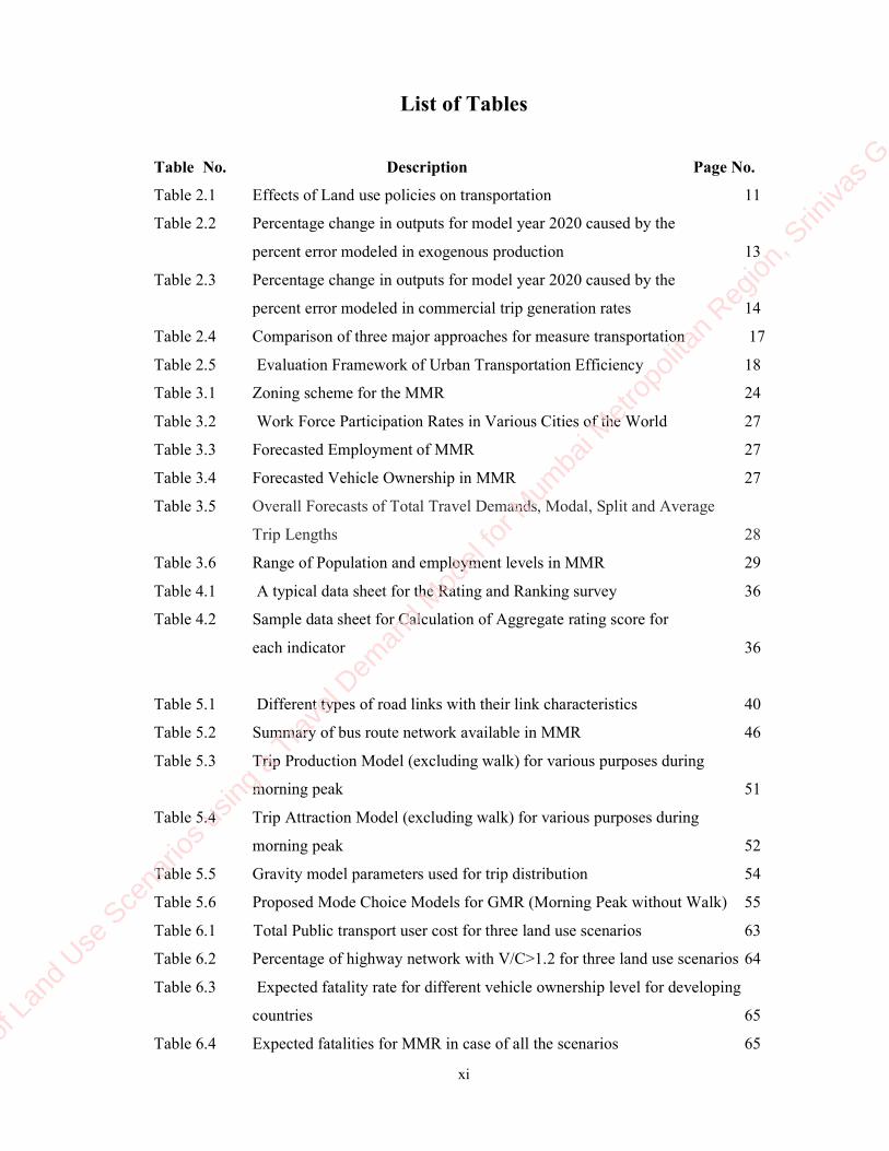
Table 2.3 Percentage change in outputs for model year 2020 caused by the
percent error modeled in commercial trip generation rates 14
Table 2.4 Comparison of three major approaches for measure transportation 17
Table 2.5 Evaluation Framework of Urban Transportation Efficiency 18
Table 3.1 Zoning scheme for the MMR 24
Table 3.2 Work Force Participation Rates in Various Cities of the World 27
Table 3.3 Forecasted Employment of MMR 27
Table 3.4 Forecasted Vehicle Ownership in MMR 27
Table 3.5 Overall Forecasts of Total Travel Demands, Modal, Split and Average
Trip Lengths 28
Table 3.6 Range of Population and employment levels in MMR 29
Table 4.1 A typical data sheet for the Rating and Ranking survey 36
Table 4.2 Sample data sheet for Calculation of Aggregate rating score for
each indicator 36
Table 5.1 Different types of road links with their link characteristics 40
Table 5.2 Summary of bus route network available in MMR 46
Table 5.3 Trip Production Model (excluding walk) for various purposes during
morning peak 51
Table 5.4 Trip Attraction Model (excluding walk) for various purposes during
morning peak 52
Table 5.5 Gravity model parameters used for trip distribution 54
Table 5.6 Proposed Mode Choice Models for GMR (Morning Peak without Walk) 55
Table 6.1 Total Public transport user cost for three land use scenarios 63
Table 6.2 Percentage of highway network with V/C>1.2 for three land use scenarios 64
Table 6.3 Expected fatality rate for different vehicle ownership level for developing
countries 65
Table 6.4 Expected fatalities for MMR in case of all the scenarios 65
Evalua
tion o
f Lan
d Use
Sce
nario
s usin
g a Trav
el Dem
and M
odel
for M
umba
i Metr
opoli
tan R
egion
, Srin
ivas G
, IIT B
omba
y

xii
Table 6. 5 Peak hour loadings by all public transport modes for P3E3 Scenario 66
Table 6. 6 Peak hour loadings by all public transport modes for P2E2 Scenario 67
Table 6. 7 Peak hour loadings by all public transport modes for P3E4 Scenario 68
Table 6. 8 Vehicle kilometers and Average trip lengths by PV and PT for all the
Scenarios 70
Table 6.9 Cost of proposed transport infrastructure for the horizon year 2031 70
Table 6.10 The summary of average ratings of the three groups of interest for
all the indicators 71
Table 6.11 The calculation sheet for computation of RTPI for all the scenarios 74
Evalua
tion o
f Lan
d Use
Sce
nario
s usin
g a Trav
el Dem
and M
odel
for M
umba
i Metr
opoli
tan R
egion
, Srin
ivas G
, IIT B
omba
y

xiii
List of Abbreviations
BEST Bombay Electric Supply and Transport Company
BRT Bus Rapid Transit
GIS Geographic Information System
GM Greater Mumbai
GT Generalized Time
IPT Intermediate Public Transport
KDMT Kalyan Dombivali Municipal Transport
MBMT Mira Bhayander Municipal Transport
MCDM Multiple Criteria Decision Making
MMR Mumbai Metropolitan Region
MMRDA Mumbai Metropolitan Regional Development Authority
MNL Multinomial Logit Model
NMMT Navi Mumbai Municipal Transport
PT Public Transport
PV Private Vehicles
RTPI Relative Transportation Performance Index
RW Relative Weighted Score
TAZ Traffic Analysis Zone
TMT Thane Municipal Transport
TRANSFORM Transportation Study for Mumbai
VMT Vehicle Miles Travelled
V/C Volume (interpreted as Demand Volume) to Capacity Ratio
VOT Value of Time
VOC Vehicle Operating Cost
Evalua
tion o
f Lan
d Use
Sce
nario
s usin
g a Trav
el Dem
and M
odel
for M
umba
i Metr
opoli
tan R
egion
, Srin
ivas G
, IIT B
omba
y

1
Chapter 1
Introduction
1.1 General
The transport of human beings represents the people’s desire to participate in various
activities like living, working, education, shopping, healthcare and recreational in various
places of any region that we concern. Similarly the transport of goods also is due to the
various activities such as production, distribution and consumption of goods in various places.
Hence the travel is the derived demand of various land use patterns of a region. It can be
easily understood that land means the spatial distribution of locations of various activities in a
region such as residential, commercial, industrial and educational etc., and the transport is the
link between them. The land use determines the magnitude, direction, purpose and spatial
distribution of travel which is to be accommodated by the overall transportation system
present in the region.
Economic development as well as industrial and social developments of any country is
very much dependent on transport infrastructure which accommodates the total travel in a
region and again which depends on land use pattern present in the region. Hence it is very
essential to study the complex inter relation between land use and transport so that
metropolitan regions and their associated transportation can be better planned through
scientific methods. The inter relationship between the urban land use and urban transport has
been recognized as the phenomenon of attention in the policy level (Gupta, 2010). Changes in
land use systems can modify the travel demand patterns and induce changes in transportation
systems. Transportation system evolution, on the other hand, creates new accessibility levels
that encourage changes in land use patterns. Hence it is assumed to be a cyclic process. Based
on this assumption many integrated land use-transport models were evolved worldwide as
well as in India to analyze the effects of land use on transport and vice versa. Even though
many integrated models were evolved, they are not best suitable for implementation for the
Indian conditions due to many reasons. Hence there is high need to study on the land use-
transport interaction in the Indian context.
1.2 Problem statement
Now a days, the urbanization is growing at an exponential rate and posses an increased
demand for the transportation facilities for the movement of man and material. The rapid
Evalua
tion o
f Lan
d Use
Sce
nario
s usin
g a Trav
el Dem
and M
odel
for M
umba
i Metr
opoli
tan R
egion
, Srin
ivas G
, IIT B
omba
y

2
growth of traffic seems to be a major problem at present for transport planner. Along with the
worldwide trend, developing countries like India are also undergoing rapid urbanization. This
shows the importance of proper planning to meet the urban transportation. The present land
use-transport integrated models explains the inter relationship between the urban land use and
transport theoretically which is practically highly impossible in the countries like India due to
many social, political and other influences. A few integrated land use transport models were
already developed in India were also failed in the applicability. Hence the alternative
approach is needed to evaluate the effect of land use on the travel pattern of the metropolitan
region like Mumbai Metropolitan Region (MMR).
As the evaluation process can be performed using a travel demand model it has to be
developed using more user friendly GIS (Geographical Information System) based
transportation planning software package. The best method should be adopted for the network
development for entire MMR without missing any possible link excepting street roads. Also
in the evaluation process, land use policies which results lowest individual motorized vehicle
need not be the best policies. There is no standardized evaluation criteria to evaluate the given
urban transportation system’s performance. Hence there is a need to study the selection
criteria of performance indicators and also to develop the criteria on which the urban
transportation system performance can be evaluated relatively.
1.3 Objectives and Scope of the Study
The main objective of the study is the evaluation of various land use or growth scenarios in
terms of mobility, accessibility, pollution and total transportation cost for the entire MMR by
developing the GIS based transportation planning model using the software package, CUBE
Voyager. With understanding the need of the project, the following sub-objectives were set
for the present study.
1. To study various methodologies for performing travel demand modeling in regional
context. To discuss the basic aspects of urban land use transport interaction and the
uncertainty of integrated land use transportation models for the evaluation of land use
scenarios in Indian conditions. Addressing the issues of selection of indicators and the
evaluation criteria.
2. Developing GIS based transportation network along with the complete data base of the
public transport services.
3. Implementing the working travel demand model for the present study area by using a
state of the art transportation modeling software.
Evalua
tion o
f Lan
d Use
Sce
nario
s usin
g a Trav
el Dem
and M
odel
for M
umba
i Metr
opoli
tan R
egion
, Srin
ivas G
, IIT B
omba
y

3
4. Selecting the performance indicator set and conducting the rating survey to assign the
relative importance to the selected indicators for the evaluation.
5. Formulation of Multi Criteria Decision Making approach for evaluating the relative
performance of urban transportation system.
6. Finally, the application of the model to evaluate the urban land use scenarios and
ranking them based on considered indices of evaluation by adopting the MCDM
technique.
1.4 Organization of the Report
The report has been divided into seven chapters. The topic has been introduced in the chapter
one highlighting the nature of the problem and its objective. Literature about Regional travel
modeling, land use transport interaction, uncertainty in integrated land use transport model in
Indian conditions and literature on evaluation of transportation system are reviewed in the
second chapter. The various aspects of study area and planning variables are discussed in the
third chapter. Fourth chapter contains the methodology to achieve the objectives for the
present study and formulated procedure for evaluation using a multi criteria decision making
approach respectively. The fifth chapter is having the contribution towards the present study
i.e. development of travel demand model is explained. The evaluation of urban transportation
system using MCDM is carried out in the chapter six. The summary and conclusions from
analysis, limitations of the study and future scope of the work are mentioned clearly in the
final chapter.
Evalua
tion o
f Lan
d Use
Sce
nario
s usin
g a Trav
el Dem
and M
odel
for M
umba
i Metr
opoli
tan R
egion
, Srin
ivas G
, IIT B
omba
y

5
Chapter 2
Literature Review
2.1 General
In this chapter basic aspects of GIS based regional travel demand modeling are discussed. The
basic interaction between the land use and transport is emphasized here to understand the inter
relation between them. Some of the existing land use transport models are reviewed and their
limitations in Indian conditions are also discussed. The different evaluation indices and
criterion for testing land use scenarios are studied in detail.
2.2 Metropolitan Regional Travel Demand Modeling
The Travel demand models are being developed since many years. Models are essentially
“decision-support tools” to assist transportation planners and policy-makers in analyzing the
effectiveness and efficiency of various transportation alternatives in terms of mobility,
accessibility, environmental and equity impacts. , it can be used for the evaluation of various
land use and transport scenarios of the region effectively. Travel demand forecasting for a
metropolitan region is definitely need to be paid attention as it consists of different sub
regions having different land use densities and different operators for the same mode of
transportation. The various regional travel demand models are summarized here. Each of
these models is having different requirements for the accuracy and usefulness of the model
outputs.
2.2.1 Baltimore Regional Travel Demand Model
(Baber & John, 2004)It is a computerized travel demand model which can simulate the
person travel and vehicle flows on the highway network and regional transit system. The
Baltimore region consists of Baltimore City and six other regions around it. The model is
developed choosing the 2000 year as the base year. The Traffic Analysis Zoning (TAZ) is
done based on the 2000 year census demographics which consists of 1463 internal TAZs and
42 external zones. Too many TAZ node numbers are used while coding the network which
can accommodate the future requirement and at the same time some lines code is inserted to
skip the process for that unused TAZs to reduce the run time for the model. MapInfo GIS and
VIPER were used to develop the highway network and public transport network coding
respectively. Here 14 different link types are used depending functionality of road. The total
Evalua
tion o
f Lan
d Use
Sce
nario
s usin
g a Trav
el Dem
and M
odel
for M
umba
i Metr
opoli
tan R
egion
, Srin
ivas G
, IIT B
omba
y

6
region has been divided into four different areas namely city centre, urban sub urban and rural
based on land use densities. The capacities and speeds for all the links are taken from HCM
2000 and they were updated on basis of land use density of the area in which they present.
The summary of the model is shown in the figure 2.1 below.
Skim Transit
Income Stratification
Trip Generation
Skim Highways
Trip Distribution
Trip Assignment
Balance Trip Table
Mode Choice
Skim Highways
Skim Transit
Trip Distribution
Income Stratification
Mode Choice
Balance Trip Table
Trip Assignment
Off - Peak Peak
Figure 2.1 The Summary of Baltimore Regional Travel demand Model (Baber & John, 2004)
The traditional sequential travel modeling steps are adopted for the study and
implemented in TP++ transportation planning software. Trip generation process is done for
different trip purposes such as, Home based other, home based work, work based other, other
based other, commercial vehicles trips, medium truck trips and heavy truck trips using
regression analysis. The generation equations are developed for all areas of the region
differently. The gravity model is used to execute trip distribution step by taking the
impedances as the travel time between the zones. The different skims are produced for six
different timings of a day. The model split step was performed for the trips of different
purposes with congested skims as input. The total trips are converted as vehicle trips and are
assigned on to the regional network to produce the link volumes, vehicle miles of travel and
volume to capacity ratios by using the equilibrium assignment model. There are two passes in
Evalua
tion o
f Lan
d Use
Sce
nario
s usin
g a Trav
el Dem
and M
odel
for M
umba
i Metr
opoli
tan R
egion
, Srin
ivas G
, IIT B
omba
y

7
the model; the AM peak period assignment produced in the first pass is used to produce
assignments in the next five time period in the second pass.
2.2.2 San Francisco Metropolitan area Travel Demand Model
The Metropolitan Transportation Commission (MTC) zonal system is 1099 regional travel
analysis zones internal to the nine-county Bay Area, and 21 external zones. The 1099 regional
travel analysis zones are based on 1990 census geography. The MTC regional transit network
includes 700+ transit lines for 25 transit operators. The modeling system includes the standard
four steps of trip generation, trip distribution, model split and trip assignment , as well as three
extra main models were; workers in household, auto ownership choice and time of the day
choice models.
Trip based versus Activity based travel demand models were discussed in the project.
It has been verbalized that market segmentation is a critical feature of the advanced trip based
travel modeling. Trips are classified as Home based work, Home based shop, home based
social/recreational, Non home based other, and Home based school. Trip generation models
include both trip production and trip attraction models. Production models are based on trips
made by households, workers or students at the home end of home-based trips. Attraction
models are based on trips made at the non home end of home-based trips. Trips as defined in
these trip generation models include non-motorized trips (bicycle, walk) as well as motorized
modes (auto, transit). With the exception of the home-based school trip generation models, all
of the new trip generation models are multiple regression in form. The home-based shop trip
generation model, in particular, is a hybrid of a cross-classification model. The usual gravity
type model is used in trip distribution step. In addition to friction factors, socio economic
adjustment factors (k-factors) are used in calibrating and validating trip distribution models.
Seven mode choice models are included in the model set, in which six are of nested logit
models and home based grade school modal split model is multinomial logit model. Departure
time choice, or time-of-day choice models, are very new to metropolitan transportation
practice. The departure time choice model included in the model system is a simple, binomial
logit choice model with two alternatives.
The utility for the off-peak alternative is defined as 0.0. Therefore, the exponentiated
utility of the off-peak alternative (exp(0)) is 1.0. In application, the probability of a home to-
work auto person trip starting in the peak period is calculated as;
Probability (Peak Start) = exp (Utility (Peak)) / [1 + exp (Utility (Peak))]
All the trips are assigned on the network as usually in trip assignment step. (Purvis, 1997)
The summary of travel demand model is shown in figure 2.2 below.
Evalua
tion o
f Lan
d Use
Sce
nario
s usin
g a Trav
el Dem
and M
odel
for M
umba
i Metr
opoli
tan R
egion
, Srin
ivas G
, IIT B
omba
y

8
Figure 2.2 Summary of San Francisco Travel demand model (Purvis, 1997)
2.3 GIS in Travel Demand Modeling
(Moorthy et al., 2003)Geographical Information System (GIS) is a preferred platform for the
travel demand modeling, because the data attributes are associated with topological object
(point, line or polygon). In GIS, information is identified according to their actual locations.
The graphical display capabilities allow visualization of different locations of traffic
generators, network and routes. The use of GIS in transportation planning will enhance the
visualization aspect and facilitate the development of decision modules for use by the
transport planners.
(Beard, 1993)Has taken the small suburban area as the study area to demonstrate the
comparative differences between GIS and Non GIS based travel modeling. The land use
characteristics in terms of developable land were forecasted by using both methods and
performed transportation planning by taking identical data set in both the methods. The results
were compared in terms of vehicle miles travelled and traffic volume on the links which have
shown the large differences. Hence we can conclude from this work that the GIS are
definitely needed for the efficient travel demand modeling.
Workers in Household Choice
Workers in Household Choice
Trip Generation
Trip Distribution
Mode Choice
Time-of-Day choice (Peak/Off-Peak)
Trip Assignment
Evalua
tion o
f Lan
d Use
Sce
nario
s usin
g a Trav
el Dem
and M
odel
for M
umba
i Metr
opoli
tan R
egion
, Srin
ivas G
, IIT B
omba
y

9
The GIS based travel models are very efficient in decision support system for
example, (Arampatzis et al., 2004) has developed the GIS integrated model, to estimate and
reproduce the traffic behavior and traffic volumes for calculating the emissions and energy
consumptions. The GIS network data base was developed in which link has the attributes like
from and to nodes, length, speed, number of lanes and capacity. The public transport service
lines data and frequencies also included GIS network. The vehicular trips are calculated
assigned on to the GIS based network. Vehicle composition and travel speeds on each link
were used calculate the emissions and energy consumption and they can be shown on the
network each link. The GIS based decision supportive system is shown in the figure 2.3.
GEO Data Central Database Transport Database
Figure 2.3 Architecture of GIS based decision supportive system (Arampatzis et al., 2004)
2.4 Land use and Transport Interaction
(Wegener & Furst, 1999)The two-way interaction between urban land use and transport
addresses the locational, mobility and accessibility responses to changes in the urban land use
and transport system at the urban or regional level. The spatial separation of human activities
creates the need for travel and goods transport is the underlying principle of transport analysis
and forecasting. Following this principle, it is easily understood that the suburbanization of
cities is connected with increasing spatial division of employees, and hence with ever
increasing mobility. However, the reverse impact from transport to land use is less well
known. There is the evolution from the medieval cities, where almost all daily mobility was
Spatial Information System
Logical data base system
Geo data update
Interface
Map based
Interface
KB data
Interface
Emission Energy
Models
Traffic
Models
Predefined Queries Knowledge Base
USER
Evalua
tion o
f Lan
d Use
Sce
nario
s usin
g a Trav
el Dem
and M
odel
for M
umba
i Metr
opoli
tan R
egion
, Srin
ivas G
, IIT B
omba
y

10
on foot, to the vast expansion of modern metropolitan areas where their massive volumes of
intraregional traffic would not have been possible without the development of first the railway
and in particular the private automobile, which has made every corner of the metropolitan
area almost equally suitable as a place to live or work. The recognition that trip and location
decisions co-determine each other and therefore transport and land-use planning needed to be
co-ordinated led to the notion of the 'land-use transport feedback cycle which is shown in the
figure 2.4.
Figure 2.4 Land use transportation feedback cycle (Wegener & Furst, 1999)
i. The distribution of land uses, such as residential, industrial or commercial, over the urban
area determines the locations of human activities such as living, working, shopping,
education and leisure.
ii. The distribution of human activities in space requires spatial interactions or trips in the
transport system to overcome the distance between the locations of activities.
iii. The distribution of infrastructure in the transport system creates opportunities for spatial
interactions and can be measured as accessibility.
iv. The distribution of accessibility in space co-determines location decisions and so results
in changes of the land-use system.
The table 2.1 explains the effects of land use on transportation well. There are other
factors also which can explain the nature of land use changes. As we are considering these
two effects only into consideration only the residential density and employment density are
taken for the review. In the table we can observe that trip frequency will not be effected up on
any land use changes. Hence we can include the trip length and mode choice excepting trip
frequency.
Evalua
tion o
f Lan
d Use
Sce
nario
s usin
g a Trav
el Dem
and M
odel
for M
umba
i Metr
opoli
tan R
egion
, Srin
ivas G
, IIT B
omba
y

11
Table 2.1 Effects of Land use policies on transportation
(Wegener & Furst, 1999)
Direction
Observed
Factor Impact on impacts
Land use
Transport
Residential
density
Trip length
Numerous studies support the
hypothesis that higher density
combined with mixed land use leads to
shorter trips. However, the impact is
much weaker if travel cost differences
are accounted for.
Trip frequency
Little or no impact observed.
Mode choice
The hypothesis that residential density
is correlated with public transport use
and negatively with car use is widely
confirmed.
Employment
density
Trip length
In several studies the hypothesis was
confirmed that a balance between
workers and jobs results in shorter
work trips, however this could not be
confirmed in other studies.Mono-
functional employment centres and
dormitory suburbs, however, have
clearly longer trips.
Trip frequency
No significant impact was found.
Mode choice
Higher employment density is likely to
induce more public transport use.
In the similar way the trasport policy changes also effect the land use patterns. i.e for
example the residential and employment density in zones along the metro corridor will be
more than that in other zones with respective to the accessibility to the bus or rail terminals.
2.4.1 Structure of Land use Transportation Interaction Models
For the purposes of longer range forecasting, in the 15 to 50 year range, such transportation
planning models need to be tied to a land use plan for the same region.
(Barra, 1989)Figure 2.5 describes a possible common structure for a typical linked
land use and transport model. The calculation sequence starts with a regional model which
consists of two linked sub models viz. a regional employment sub model and a demographic
Evalua
tion o
f Lan
d Use
Sce
nario
s usin
g a Trav
el Dem
and M
odel
for M
umba
i Metr
opoli
tan R
egion
, Srin
ivas G
, IIT B
omba
y

12
sub model, which together perform the calculation of the total population and employment for
the region.
Regional level
Urban activity
Level
Urban Transport
Level
Figure 2.5 The general structure of integrated land use and transport model (Barra, 1989)
The next stage corresponds to the location of activities within the urban area or in the
region and consists of the location of basic employment, floor space, residential population
and service employment from the totals generated by the regional model. These in turn are
input to the transportation model, consisting of four stages; trip generation trip distribution,
model split, trip assignment and generalized costs or skims.
From the generalized cost calculations, two main feedbacks are recognized. The first
goes to the trip distribution stage as the congestion builds up in certain parts of the network,
the trip distribution step is affected and probabilities choosing the each mode can change. This
feedback is equivalent to equilibrium between supply and demand of the transport. This
equilibrium is assumed to takes place instantaneously i.e. no time lag is required.
The second feedback goes back to the location of activities, affected by the changes in
the generalized cost of the travel between the zones. This second loop is assumed to takes
place more slowly, because activities will take some to adapt to the changes in the changes in
Regional Employment
Model for all periods
Demographic Model for
all periods
Basic employment
location model
Location of floor space, residents
and service employment
Trip generation models
Trip distribution and
model split models
Trip assignment model
Travel time and
generalized costs
Evalua
tion o
f Lan
d Use
Sce
nario
s usin
g a Trav
el Dem
and M
odel
for M
umba
i Metr
opoli
tan R
egion
, Srin
ivas G
, IIT B
omba
y

13
the accessibility. It is easily understood that, the two key elements that relate land use and
transportation are trip generation and generalized cost.
2.4.2 Uncertainty in Integrated Land use Transport Models
Johnston & Clay (2005) Integrated land use and transportation models are typically given
precise inputs and return precise outputs. The authors have introduced the uncertainty into the
inputs of an integrated land use and travel demand model to determine the effect of uncertain
inputs on the model outputs. In the uncertainty analysis, only selected variables are varied
based on their sources of uncertainty in the model. Sacramento of California is considered as
the study area which is having the population of 1.9 millions in the base year 2000. The
MEPLAN integrated land use transport model is used for the demonstration of uncertainty.
Exogenous production, commercial trip rates and concentration parameter are varied plus or
minus 10, 25, and 50% which indirectly represents the errors in their sources such as forecasts
of population and employment. The results were demonstrated through the results shown in
following table 2.2 and table 2.3.
Table 2.2 Percentage change in outputs for model year 2020 caused by the percent error
modeled in exogenous production (Johnston & Clay, 2005)
Exogenous
Production (%)
VMT
(%)
SOV mode
share (%)
SOV mode share
for work trips (%)
Total number of
SOV trips (%)
+10 1.64 -0.96 -0.51 2.37
-10 -2.87 0.57 0.82 -2.81
+20 4.36 -1.87 -1.56 6.83
-25 -6.13 1.13 1.40 -7.38
+50 8.61 -3.16 -3.44 13.11
-25 -12.60 3.15 4.38 -14.23
Vehicle miles traveled (VMT) and the number of trips are the most vulnerable of the
outputs monitored to uncertain population and employment forecasts. This is expected. The
number of trips per household is a fixed relationship in this model, hence any increase in the
number of households will be accompanied by an increase in the number of trips. The number
of miles traveled will vary with the number of trips and with average speeds.
Single occupant vehicle (SOV) mode shares change very little even with 50% swings
in the forecasts of exogenous demand and they change in the opposite direction to VMT and
total number of trips. As population goes up, so does VMT and the number of trips, which
causes increased congestion and a lower mode share for single occupant vehicles. Figure 2.6
shows the impact across model years of uncertainty in exogenous production on outputs.
Evalua
tion o
f Lan
d Use
Sce
nario
s usin
g a Trav
el Dem
and M
odel
for M
umba
i Metr
opoli
tan R
egion
, Srin
ivas G
, IIT B
omba
y
14
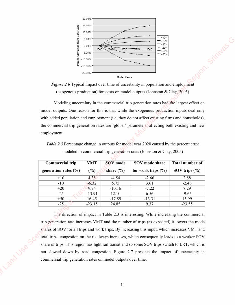
Figure 2.6 Typical impact over time of uncertainty in population and employment
(exogenous production) forecasts on model outputs (Johnston & Clay, 2005)
Modeling uncertainty in the commercial trip generation rates had the largest effect on
model outputs. One reason for this is that while the exogenous production inputs deal only
with added population and employment (i.e. they do not affect existing firms and households),
the commercial trip generation rates are ‘global’ parameters, affecting both existing and new
employment.
Table 2.3 Percentage change in outputs for model year 2020 caused by the percent error
modeled in commercial trip generation rates (Johnston & Clay, 2005)
Commercial trip
generation rates (%)
VMT
(%)
SOV mode
share (%)
SOV mode share
for work trips (%)
Total number of
SOV trips (%)
+10 4.35 -4.54 -2.66 2.88
-10 -6.32 5.75 3.61 -2.46
+20 9.74 -10.16 -7.22 7.29
-25 -13.91 12.10 6.56 -9.65
+50 16.45 -17.89 -13.31 13.99
-25 -23.15 24.85 9.37 -23.55
The direction of impact in Table 2.3 is interesting. While increasing the commercial
trip generation rate increases VMT and the number of trips (as expected) it lowers the mode
shares of SOV for all trips and work trips. By increasing this input, which increases VMT and
total trips, congestion on the roadways increases, which consequently leads to a weaker SOV
share of trips. This region has light rail transit and so some SOV trips switch to LRT, which is
not slowed down by road congestion. Figure 2.7 presents the impact of uncertainty in
commercial trip generation rates on model outputs over time.
Evalua
tion o
f Lan
d Use
Sce
nario
s usin
g a Trav
el Dem
and M
odel
for M
umba
i Metr
opoli
tan R
egion
, Srin
ivas G
, IIT B
omba
y

15
Figure 2.7 Typical impacts over time of uncertainty in commercial trip generation rates on
model outputs (Johnston & Clay, 2005)
Here we can easily understand that the amount of error in the VMT outputs may be
greater than the VMT differences produced by alternative policies (or transportation
improvements/investments). If this is the case, the land use plans cannot be evaluated or
ranked correctly.
2.5 Evaluation indicators for the land use scenarios
(Littman, 2011) has mentioned that the sustainable planning decisions depend on the how the
transportation systems performance is measured with some indicators. The indicators are
having many uses in planning and management. This data helps in indentifying the problems,
accessing the alternative options to solve them, setting the performance targets and evaluate a
particular jurisdiction in the study area or whole region. The type of indicators that we chose
will definitely influence on the results analysis because a particular policy may rank high with
one set of indicator set but it rank very low with another set of indicators. Hence it is
suggested to take at most care while selecting the performance indicators.
The author also specified standard definitions as below which have given motivation
to develop the methodology which is used in the present study.
Target: A specified, realistic, measurable objective
Indicator: a variable selected and defined to measure the progress towards the
objective
Indicator type: nature of data used by the indicator (quantitative, qualitative, absolute
or relative)
Indicator set: a group of indicators selected to measure the comprehensive progress
toward the goals
Index: a group of indicators aggregated to form a single value
Evalua
tion o
f Lan
d Use
Sce
nario
s usin
g a Trav
el Dem
and M
odel
for M
umba
i Metr
opoli
tan R
egion
, Srin
ivas G
, IIT B
omba
y

16
2.5.1 Guide lines for selecting the indicators
Littman, 2011 has suggested a few guidelines or precautions to select the proper indicator set
while evaluating the transportation system performance.
i. All the indicators are selected based on their usefulness in decision making in
transportation planning and also on the ease of collection of data or measuring them.
ii. An indicator which focuses too much on one type of impact may overlook the other
impacts, so that the decisions resulted cannot be optimal. Hence it is very important to
understand the perspectives, assumptions and limitations of each indicator in
representing the particular impact.
iii. The indicators are evaluated for each jurisdiction wise to take the better decisions in
transportation planning, and also the indicators should be comparable with the other
jurisdictions in terms of performance.
iv. Indicators should be easy to understand.
v. The maximum possible indicators are used in the set which can well represent the
impacts or performance as well as which can quantifiable easily the available
resources of information.
(Littman, 2008)There are different perspectives with different measures of transportation
system in a region. There exist three approaches to measuring transportation system
performance.
i. Traffic-based measurements (such as vehicle trips, traffic speed and roadway level of
service) evaluate motor vehicle movement.
ii. Mobility-based measurements (such as person-miles, door-to-door traffic times and
ton miles) evaluate person and freight movement.
iii. Accessibility-based measurements (such as person-trips and generalized travel costs)
evaluate the ability of people and businesses to reach desired goods, services and
activities.
Accessibility is the ultimate goal of most transportation and so is the best approach to use.
There is no single way to measure transportation performance that is both convenient and
comprehensive. Transportation professionals should become familiar with the various
measurement methods and units available, learn about their assumptions and perspectives, and
help decision makers to understand how they are best used to accurately evaluate problems
and solutions.
Evalua
tion o
f Lan
d Use
Sce
nario
s usin
g a Trav
el Dem
and M
odel
for M
umba
i Metr
opoli
tan R
egion
, Srin
ivas G
, IIT B
omba
y

17
Conventional ways of measuring transportation system performance, such as roadway
Level of Service and traffic speed, tend to favor vehicle travel over other forms of access.
Only by developing better methods of measuring mobility and accessibility, more accessible
land use patterns will be recognized. The following table 2.4 compares the compares the three
major approaches for measuring transportation.
The transportation system performance can also be measured in mode share for different
modes, V/C (Volume to Capacity ratio) ratios for all links of the network and level of service
for the total network.
Table 2.4 Comparison of three major approaches for measure transportation (Littman, 2008)
Traffic Mobility Accessibility
Definition of
Transportation
Vehicle travel. Person and goods
movement.
Ability to obtain
goods, services and
activities.
Unit of measure Vehicle-miles and
vehicle-trips
Person-miles, person-
trips and ton-miles.
Trips.
Modes
considered
Automobile and truck. Automobile, truck and
public transit.
All modes, including
mobility substitutes
such as
telecommuting.
Common
performance
indicators
Vehicle traffic
volumes and speeds,
roadway Level of
Service, costs per
vehicle- mile, parking
convenience.
Person-trip volumes
and
speeds, road and transit
Level of Service, cost
per person- trip, travel
convenience.
Multi-modal Level of
Service, land use
accessibility,
generalized cost to
reach activities.
Assumptions
concerning what
benefits
consumers.
Maximum vehicle
mileage and speed,
convenient parking,
low vehicle costs.
Maximum personal
travel and goods
movement.
Maximum transport
options, convenience,
land use accessibility,
cost efficiency.
Consideration of
land use.
Favors low-density,
urban fringe
development patterns.
Favors some land use
clustering, to
accommodate transit.
Favors land use
clustering, mix and
connectivity.
Evalua
tion o
f Lan
d Use
Sce
nario
s usin
g a Trav
el Dem
and M
odel
for M
umba
i Metr
opoli
tan R
egion
, Srin
ivas G
, IIT B
omba
y

18
Traffic Mobility Accessibility
Favored
transport
improvement
strategies
Increased road and
parking capacity,
speed and safety.
Increased transport
system capacity,
speeds and safety.
Improved mobility,
mobility substitutes
and land use
accessibility.
(YUAN, 2003) has considered that the urban transportation system performance is the
key factor in determining the capability of urban transportation system and the balance
between the travel demand and supply. The impact factors of urban transportation efficiency
are mainly divided into four aspects such as urban land use pattern, transportation
infrastructure and traffic management system. The hierarchical evaluation framework of
urban transportation efficiency is proposed which is shown in the table 2.5.
Table 2.5 Evaluation Framework of Urban Transportation Efficiency (YUAN, 2002)
Type of
factors Index level _1 Index level _2 Index level _3
Urban layout
and land-use
pattern
A1—population density in downtown areas
A2-- ratio of job units to residential population
A3-- ratio of population density in downtown areas to that in suburbs
A4-- relative radius of transportation within 0.5, 1, 2 hours
Urban
transportation
structure
A5-- share of urban public transportation modes
Urban
transportation
infrastructure
A6--
efficiency of
road
infrastructure
B1-- ratio of Average Travel Speed (ATS) to designed
road speed
B2 -- ratio of V/C
B3 -- ratio of traffic volume in peak hours to AADT
A7 --
efficiency of
parking
infrastructure
B4--ratio of average parking volume in peak hours to
designed capacity
B5-- ratio of average daily occupancy time of each berth
B6-- ratio of average daily parking number of each berth
A8--
efficiency of
urban
transportation
vehicles
B7 --
efficiency of
bus systems
C1 -- average load factor of bus systems
C2 --average area of road occupancy per
passenger of bus systems
C3 – average daily overload duration of bus
systems
B8--
efficiency of
urban rail
systems
C4 -- average load factor of rail systems
C5 -- average area of carriage occupancy
per passenger of rail systems
C6-- average daily overload duration of rail
systems
B9 -- proportion of congested intersections without signal
Urban traffic A9 – status of control during peak hours
Evalua
tion o
f Lan
d Use
Sce
nario
s usin
g a Trav
el Dem
and M
odel
for M
umba
i Metr
opoli
tan R
egion
, Srin
ivas G
, IIT B
omba
y

19
Type of
factors Index level _1 Index level _2 Index level _3
management traffic
congestion
B10 --proportion of congested intersections controlled by
traffic signal during peak hours
B11--average intersections daily congestion duration of
main intersections
A 10--status of
traffic safety
B12 -- death toll per 10000 PCU
B13 -- death toll per 1 mil. (PCU˙Km)
Energy
reservation A11-- average energy consumption per capita in urban transportation
systems
Environment
protection
A12-- share of air pollution
A13-- share of noises pollution
The author also has clearly expressed the problems encountering in the evaluation of urban
transportation infrastructure efficiency is that there is not a determined and absolute way to be
referred and the uncertainty of evaluation criteria is the most important problem to be solved.
The fuzzy theory is adopted here to reduce the uncertainty and the three cities (Guangzhou,
Shanghai and Beijing) are compared w.r.t. the relative transportation system performance.
The more practical performance indicators suitable for evaluating the proposed transportation
system’s performance are given below by Litman, 2011.
• Awareness – the portion of potential users who are aware of a program or service.
• Participation – the number of people who respond to an outreach effort or request to
participate in a program.
• Utilization – the number of people who use a service or alternative mode.
• Mode split – the portion of travelers who use each transportation mode.
• Mode shift – the number or portion of automobile trips shifted to other modes.
• Average Vehicle Occupancy (AVO): Number of people traveling in private vehicles
divided by the number of private vehicle trips. This excludes transit vehicle users and
walkers.
• Average Vehicle Ridership (AVR): All person trips divided by the number of private
vehicle trips. This includes transit vehicle users and walkers.
• Vehicle Trips or Peak Period Vehicle Trips: The total number of private vehicles
arriving at a destination (often called “trip generation” by engineers).
• Vehicle Trip Reduction – the number or percentage of automobiles removed from
traffic.
• Vehicle Miles of Travel (VTM) Reduced – the number of trips reduced times average
trip length.
Evalua
tion o
f Lan
d Use
Sce
nario
s usin
g a Trav
el Dem
and M
odel
for M
umba
i Metr
opoli
tan R
egion
, Srin
ivas G
, IIT B
omba
y

20
• Energy and emission reductions – these are calculated by multiplying VMT reductions
times average vehicle energy consumption and emission rates.
• Accessibility (ability to reach desired services and activities), including the travel time
and costs required by various users to reach activities and destinations such as work,
education, public services and recreation
• User Evaluation – Overall user satisfaction with their transportation system.
Planners should identify appropriate indicators that measure progress toward stated goals and
objectives, taking into account the quality of available data and the costs of collecting any
additional data.
(Zegras, 2006) has explained the role of performance indicators, evaluation criteria in a very
nice manner through a flow chart which is shown in the figure 2.8.
Figure 2.8 The role of indicators in a transportation planning process
(Zegras, 2006) also presents the Sustainability Indicator Prism that innovatively represents the
hierarchy of goals, indexes, indicators, and raw data as well as the structure of
multidimensional performance measures (Zegras, 2006). As shown in Figure 2.9, the top of
the pyramid represents the community goals and vision, the second layer represents a number
of composite indexes around the selected themes, third layer represents indicators or
performance measures building from raw data at the bottom of the pyramid.
Figure 2.9 sustainability indicator prism (Zegras, 2006)
Evalua
tion o
f Lan
d Use
Sce
nario
s usin
g a Trav
el Dem
and M
odel
for M
umba
i Metr
opoli
tan R
egion
, Srin
ivas G
, IIT B
omba
y

21
2.5.2 Multiple Criteria Decision Making in Transportation Planning
The multidimensional nature of sustainability indicates that multi criteria or multi objective
methods would be more appropriate for sustainability assessments than single-
criterion/single-objective methods. This section first reviews multiple criteria decision making
(MCDM) methods in general and identifies a number of MCDM applications to transportation
planning decision making. Multi-criteria decision making (MCDM) is one of the established
branches of Decision Theory, and it is especially useful when making preference-based
decisions over available alternatives that are characterized by multiple, usually conflicting,
attributes
(Hwang and Yoon, 1981; Triantaphyllou, 2000) Unlike single-objective decision-making
techniques, such as benefit-cost or cost-effectiveness analysis, MCDM approaches can take
into account a wide range of differing, yet relevant criteria. Even though these criteria cannot
always be expressed in monetary terms, as is the case with many externalities, comparisons
can still be based on relative priorities. MCDM methods are generally divided into (1) multi-
objective decision making (MODM) that studies decision problems with a continuous
decision space and (2) multi attribute decision making (MADM).
Because the transportation planning process includes many different objectives or attributes
and reflects the interests of a wide range of stakeholders, appropriate techniques need to
incorporate these multiple and conflicting objectives into the assessment process. Moreover,
decision-making in the context of sustainable transportation should involve the evaluation of a
discrete set of alternatives while simultaneously considering conflicting objectives. This
section identifies relevant international studies that apply different MCDM methods to
metropolitan transportation planning and decision making.
The research trends indicate that MCDM methods have been often applied to project-level
studies since the early 1980s. MCDM applications to broader scope analyses, such as the
evaluation of transportation plans or policies, are more recent research trends. One of the most
common methodologies of MCDM is Saaty’s Analytic Hierarchy Process (AHP) developed in
1970s to provide a systematic approach to setting priorities and decision making based on
pairwise comparisons between criteria. Another recent trend includes an embracement of
different types of “fuzzy” multi criteria decision making approaches. These fuzzy-type
MCDM methods attempt to cater for uncertainty, vagueness, or fuzziness commonly inherent
in human decision making due to a lack of information or constraints in human thinking.
Some other initiatives make progress by combining the AHP method with different types of
fuzzy MCDM methods. The following two paragraphs describe some examples of relevant
Evalua
tion o
f Lan
d Use
Sce
nario
s usin
g a Trav
el Dem
and M
odel
for M
umba
i Metr
opoli
tan R
egion
, Srin
ivas G
, IIT B
omba
y

22
studies that apply the AHP method and fuzzy-type MCDM methods, respectively, in
transportation decision making.
2.5.3 Inferences from the literature
The existing indicator systems reveal that operationally, transportation system performance is
largely being measured by transportation system effectiveness and efficiency as well as the
environmental impacts of the system. The application of a multiple criteria decision making
(MCDM) approach in the sustainability evaluation framework is broadly applicable. Most
analytical models of sustainability are based on the multidimensional themes of economic,
environmental, and social impacts, indicating that a robust method should at the minimum
consider these dimensions as decision making criteria. Thus, multicriteria/multiobjective
methods seem to be better suited to sustainability assessments than single-criterion/single
objective methods. Common multiple criteria decision making (MCDM) methods were first
reviewed in general, and their applications to transportation planning and decision making
identified. The chapter 5 demonstrates a proposed formulation of the multiple criteria decision
making (MCDM) approach for evaluating competing land use scenarios and identifying
superior alternatives.
2.6 Summary
The stated of art in regional travel modeling is reviewed here by taking two regional travel
models as case studies. In both the models the traditional travel modeling technique is used.
Advantages of advanced trip based modeling are pointed out over activity based modeling.
After that the importance of GIS in Travel demand modeling is discussed. Then the concept
of land use transport interaction and outline of land use transport modeling are reviewed. The
uncertainty in integrated land use transport models is highlighted by taking one case study.
Hence it is proposed that the traditional scenario based approach is adopted for the present
study for the evaluation of land use scenarios. The evaluation indices also are briefly outlined
here. The next chapter explains the study area features and planning variables for the present
study.
Evalua
tion o
f Lan
d Use
Sce
nario
s usin
g a Trav
el Dem
and M
odel
for M
umba
i Metr
opoli
tan R
egion
, Srin
ivas G
, IIT B
omba
y

23
Chapter 3
Study Area and Planning Variables
3.1 General
Mumbai Metropolitan Region (MMR)/Mumbai Metropolitan Area, comprising of a municipal
corporations, councils, and rural areas is the largest urban agglomeration in India. The MMR
is spread over an area of 4355 square kilometers and has a population of approximately 16.73
million according to 2001 census which is accounting for 20% population of total
Maharashtra and about 2% population of India. It is estimated to grow to 23 million by 2011
and 34 million by 2031. Primary among the constituents of MMR is the Greater Mumbai
which is referred as financial capital of India, hence the employment is very much high in
MMR. About 0.7 million people enter the Greater Mumbai daily in the morning peak period.
The economic and transportation perspective in the different regions in the MMR are
functioning as a single entity with people travelling between different municipal areas for
work, education, shopping and personal needs.
3.2 Study Area
The Mumbai Metropolitan Region is the metropolitan area consisting of the metropolis of
Mumbai and its satellite towns. Developing over a period of about 20 years, it consists of
seven municipal corporations and fifteen smaller municipal councils. The entire area is
overseen by the Mumbai Metropolitan Region Development Authority (MMRDA)The study
area consists of 4 districts of Maharashtra in which Mumbai City and Mumbai suburbs are
completely included and parts of Thane and Raigarh. The Mumbai Metropolitan Region
(MMR) is one of the fastest growing metropolises in India. With a population of 17.7 Million
(Census, 2001), it is ranked as the sixth largest metropolitan region in the world. The
composition is given in the figure 3.1 as well as in table 3.1.
Evalua
tion o
f Lan
d Use
Sce
nario
s usin
g a Trav
el Dem
and M
odel
for M
umba
i Metr
opoli
tan R
egion
, Srin
ivas G
, IIT B
omba
y

24
Figure 3.1 Sub Regions of MMR (TRANSFORM, 2005)
3.3 Zoning System
Any transportation model requires the study area to be divided into the zones i.e. Traffic
Analysis Zones. As per TRANSFORM, 2005 the MMR has been divided into 1037 zones. In
all there are 1030 internal zones are within MMR and there are 7 external zones which are
within Maharashtra but outside of MMR. All these zones are systematically numbered which
have been shown in the table 3.1.
Table 3.1 Zoning scheme for the MMR (TRANSFORM, 2005)
S.No Name of area Number of TAZ Zone Coding
1
MCGM 577
1-577 Island 232
Western Suburb 228
Eastern Suburb 117
2 Mira-Bhayender 26 578 - 603
3 Thane 95 671 - 765
4 Nallasopara 13 631 - 643
5 Navgarh-Manikpur 6 625 - 630
6 Vasai 21 604 - 624
7 Virar 27 644 - 670
8 Navi Mumbai 66 766 - 831
Evalua
tion o
f Lan
d Use
Sce
nario
s usin
g a Trav
el Dem
and M
odel
for M
umba
i Metr
opoli
tan R
egion
, Srin
ivas G
, IIT B
omba
y

25
S.No Name of area Number of TAZ Zone Coding
9 Panvel 8 842 - 849
10 Uran 2 850 -851
11 Rest of CIDCO 10 832 - 841
12 Kalyan-Dombiviali 54 851 - 905
13 Ulhasnagar 25 906 - 930
14 Ambernath 14 931 - 944
15 Bhiwandi - Nizampur 28 951 - 978
16 Kulgaon - Badlapur 6 945 - 950
17 Alibag 3 979 -981
18 Pen 6 982 - 987
19 Khopoli 5 988 - 992
20 Karjat 4 993 - 996
21 Matheran 1 997
22 Rural areas 33 998 - 1030
23 External zones 7 1031 - 1037
3.4 Planning Variables
Transportation is the movement of people or goods from an origin to destination. This pattern
of movement may vary with time and region. To capture these travel patterns and to
appropriately represent in the model, the characteristics of the origin and destination zones
should be necessarily studied. The number of planning parameters or variables used for the
modeling may vary with the study area, level of details required for the modeling and purpose
of modeling.
Earlier comprehensive transportation studies had been carried out by M/S Wilbur
smith & Associates in 1963, Central Road Research Institute (CRRI) in 1983 and by W.S.
Atkins in 1994. They have proposed various road development plans like developing arterials
and expressways. The planning parameters used in Wilbur smith were total population,
employment, and vehicle ownership and population density. In this study the MMR has been
divided into 139 zones. In the CRRI study total population, resident workers, resident
students, total employment, industrial employment were taken as planning variables. In this
study, MMR was divided into 99 zones.
Besides population, employment and its sub categories no other parameter have been
taken for planning by any of the studies.
The travel demand in an area depends on land use distribution and its intensity. The
variables that describe the travel demand traditionally have been the population, employment
and vehicle ownership. Population, employment and vehicle ownership in greater Mumbai
and their projection into the future has been taken from the Transform study (2005). The
Evalua
tion o
f Lan
d Use
Sce
nario
s usin
g a Trav
el Dem
and M
odel
for M
umba
i Metr
opoli
tan R
egion
, Srin
ivas G
, IIT B
omba
y

26
zonal planning parameters considered from the Transform study for Travel demand modeling
are,
i. Population (POP)
ii. Resident Worker – Office (RWF)
iii. Resident Worker - Industry category (RWI)
iv. Resident Worker – Other (RWO)
v. Resident Student (RS)
vi. Office Jobs/Employment (OJ)
vii. Industry Jobs/Employment (IJ)
viii. Other Jobs/Employment (OTJ)
The planning variables for the year 2005, 2016, and 2031 and the aggregate total population
and employment are taken from TRANSFORM Study and updated to base year.
Population
The estimation of population for the total MMR is shown the figure 3.2.
Figure 3.2 Forecasted Population of MMR from 1971 to 2031 (TRANSFORM, 2005)
Employment
Examples of the employment participation rates in some of the larger cities of the world are
shown in table 3.2. The relatively low employment participation rate in the MMR is largely a
reflection of the low participation rates by females in the workforce. An increase in the per
capita employment rate (0.37 to 0.45) over the next 25 years is considered reasonable. This
would mean a 2031 employment level of 15.3 million or a doubling of employment over
2005. The female employment rate in the MMR is currently at 0.12 compared to 0.56 of
males. In order to increase the overall participation rate to 0.45 and assuming a 5% increase in
male participation the female rate would have to increase to 0.28. This increase is considered
both achievable and desirable over the next 25 years particularly with greater levels of female
enrollment in schools. (TRANSFORM, 2005)
Evalua
tion o
f Lan
d Use
Sce
nario
s usin
g a Trav
el Dem
and M
odel
for M
umba
i Metr
opoli
tan R
egion
, Srin
ivas G
, IIT B
omba
y

27
Table 3.2 Work Force Participation Rates in Various Cities of the World (TRANSFORM,
2005)
Name of city Work force participation rate
Bangkok 0.53
Shanghai 0.59
Mexico City 0.40
Bogota 0.41
Seoul 0.48
Sap Paulo 0.41
London 0.53
Frankfurt 0.81
Hong Kong 0.47
Tokyo 0.54
Mumbai 2005
Estimate for MMR (2031)
0.37
0.45
The rest of the MMR i.e. MMR excluding Greater Mumbai had an employment of 6.09 lakhs
in 87,720 establishments in 1980 which has increased to 7.97 lakhs and 1.62 lakhs
respectively in 1990. Bhiwandi urban in 1990 has the highest employment of 1.71 lakhs
followed by 1.54 lakhs in Thane and 1.32 lakhs in Kalyan. The projected employment in
MMR is shown in the table 3.3.
Table 3.3 Forecasted Employment of MMR (TRANSFORM, 2005)
Factor 1971 1981 1991 2001 2011
Employment 1760500 2822300 3228763 4139521 543452
Vehicle ownership
The increase in private vehicle ownership during the period 1996-2005 in GMR is from 52 to
82 where as private vehicle ownership in MMR is increases from 50 to 95. The private
vehicle ownership in the rest of region is more than GMR. The phenomenon may be due to
high accessibility of IPT in GMR. Forecasted growth of vehicle ownership (per 10000
population) presented in the table was taken from transform study and are shown in Table 3.4
Table 3.4 Forecasted Vehicle Ownership in MMR per 1000population (TRANSFORM, 2005)
Year GMR Rest of MMR MMR
2006 95 134 110
2011 112 180 139
2016 132 228 171
2021 153 270 204
2026 175 304 236
2031 197 329 266
Evalua
tion o
f Lan
d Use
Sce
nario
s usin
g a Trav
el Dem
and M
odel
for M
umba
i Metr
opoli
tan R
egion
, Srin
ivas G
, IIT B
omba
y
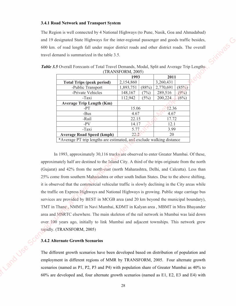
28
3.4.1 Road Network and Transport System
The Region is well connected by 4 National Highways (to Pune, Nasik, Goa and Ahmadabad)
and 19 designated State Highways for the inter-regional passenger and goods traffic besides,
600 km. of road length fall under major district roads and other district roads. The overall
travel demand is summarized in the table 3.5.
Table 3.5 Overall Forecasts of Total Travel Demands, Modal, Split and Average Trip Lengths
(TRANSFORM, 2005)
1993 2011
Total Trips (peak period) 2,154,860 3,260,431
-Public Transport 1,893,751 (88%) 2,770,691 (85%)
-Private Vehicles 148,167 (7%) 289,516 (9%)
-Taxi 112,942 (5%) 200,224 (6%)
Average Trip Length (Km)
-PT 15.06 12.36
-Bus 4.67 4.67
-Rail 22.15 17.72
-PV 14.17 12.1
-Taxi 5.77 3.99
Average Road Speed (kmph) 22.2 20
*Average PT trip lengths are estimated, and exclude walking distance
In 1993, approximately 30,116 trucks are observed to enter Greater Mumbai. Of these,
approximately half are destined to the Island City. A third of the trips originate from the north
(Gujarat) and 42% from the north-east (north Maharashtra, Delhi, and Calcutta). Less than
25% come from southern Maharashtra or other south Indian States. Due to the above shifting,
it is observed that the commercial vehicular traffic is slowly declining in the City areas while
the traffic on Express Highways and National Highways is growing. Public stage carriage bus
services are provided by BEST in MCGB area (and 20 km beyond the municipal boundary),
TMT in Thane , NMMT in Navi Mumbai, KDMT in Kalyan area , MBMT in Mira Bhayander
area and MSRTC elsewhere. The main skeleton of the rail network in Mumbai was laid down
over 100 years ago, initially to link Mumbai and adjacent townships. This network grew
rapidly. (TRANSFORM, 2005)
3.4.2 Alternate Growth Scenarios
The different growth scenarios have been developed based on distribution of population and
employment in different regions of MMR by TRANSFORM, 2005. Four alternate growth
scenarios (named as P1, P2, P3 and P4) with population share of Greater Mumbai as 40% to
60% are developed and, four alternate growth scenarios (named as E1, E2, E3 and E4) with
Evalua
tion o
f Lan
d Use
Sce
nario
s usin
g a Trav
el Dem
and M
odel
for M
umba
i Metr
opoli
tan R
egion
, Srin
ivas G
, IIT B
omba
y

29
employment share of Greater Mumbai as 33% to 75% are developed. The totals of sixteen
combinations of these scenarios are generated. Based on distribution of population and
employment among various areas in MMR, the other planning parameters are deduced and
are used in the model. The same is shown in the table 3.6. The sixteen possible combinations
of these scenarios are formed in which three short listed scenarios (P2E2, P3E3 and P3E4) are
evaluated in the present study.
Table 3.6 Range of Population and employment levels in MMR (TRANSFORM,2005)
CLUSTERS
POPULATION (IN LAKHS) EMPLOYMENT (IN LAKHS)
2005 2031
P1
2031
P2
2031
P3
2031
P4 2005
2031
E1
2031
E2
2031
E3
2031
E4
Island 33.9 54.4 47.8 40.8 37.4 22.6 40.3 36.2 28.4 20.5
Western 56.3 91.8 78.8 71.5 61.3 23.0 48.0 41.5 30.8 19.3
Eastern 38.4 61.2 53.6 47.6 40.8 11.4 21.5 19.3 14.4 11.1
Total Greater Mumbai 128.6 207.4 180.2 159.9 139.5 56.9 109.8 97.0 73.5 51.0
Thane 15.2 16.0 26.2 26.2 26.2 3.9 7.2 9.9 13.3 14.9
Navi Mumbai/CIDCO 15.0 22.8 33.0 33.0 39.8 5.9 10.0 12.1 17.5 22.3
Mira Bhayandar 6.3 13.6 13.6 13.6 13.6 1.5 2.6 2.5 3.9 5.0
Kalyan Dombivali 23.0 29.6 41.5 46.7 46.7 4.8 7.4 9.4 13.5 14.0
Bhiwandi 6.8 13.1 13.1 13.1 13.1 2.1 4.3 4.3 4.5 4.5
Vasai-Virar 7.1 13.1 13.1 14.8 18.2 1.6 2.4 4.1 7.2 9.1
Pen-SEZ 1.2 18.8 13.7 27.2 37.4 0.2 8.5 12.8 18.6 31.2
Rural 4.9 5.6 5.6 5.6 5.6 0.7 0.8 0.9 1.1 1.1
Total 208.2 340.0 340.0 340.0 340.0 77.6 153.0 153.0 153.0 153.0
3.5 Summary
The basic demographic aspects of the study area, outline of previous transport studies and
basic planning variables and their statistics are discussed here. The population and
employment related planning variables are only considered for the study. The different of land
use growth scenarios are also presented here, out of which the three short listed scenarios
adopted directly for the present study. Zoning system and its numbering which is adopted in
the present study is also given this chapter. The same zoning system is followed in our
modeling process also.
Evalua
tion o
f Lan
d Use
Sce
nario
s usin
g a Trav
el Dem
and M
odel
for M
umba
i Metr
opoli
tan R
egion
, Srin
ivas G
, IIT B
omba
y

30
Chapter 4
Methodology
4.1 General
This chapter describes the methodology adopted for evaluation of land use scenarios with the
development of travel demand model in the study area. Comprehensive Transportation study
for Mumbai Metropolitan (TRANSFORM-2005) is the starting point for this present
modeling exercise. The methodology adopted for evaluation of land use scenarios consists of
the following steps,
- Development of highway network and public transit network
- Updating the base year travel pattern
- Horizon year Travel Demand Model development
- Development of indices for the evaluation of different land use scenarios
- Evaluation of land use land use scenarios using the travel demand model w.r.t.
proposed transportation system performance perspective
The following sections briefly describe these steps.
4.2 Development of highway and public transit network
The network is developed from different shape files for all types of road network which are
available from MMRDA which have been used also for the TRANSFORM Study. The
network information generated was strategic consisting of major roads in the study area. The
road network was properly connected to all the zone centroids by means of centroid
connectors.
4.2.1 Highway network development
The total highway network is developed from the shape files in GIS based software tools. The
collection of shape files consists of local roads, arterials, sub-urban, metro and mono rail links
individually for existing and proposed links. The attributes associated with the shape file are
inadequate for the network development. Hence the required attributes are added to the
corresponding individual shape files using ArcGIS. Then they are converted to geographic
files and then they have been merged using TransCAD to form the single shape file consisting
of all the existing and proposed links. The network is developed from the resultant shape file
Evalua
tion o
f Lan
d Use
Sce
nario
s usin
g a Trav
el Dem
and M
odel
for M
umba
i Metr
opoli
tan R
egion
, Srin
ivas G
, IIT B
omba
y
31
using CUBE Base software. Now the resultant network file is lacking of centriod connectors
which can be developed through overlapping of network on the shape file zonal layers but
zonal numbers will be different from the same in TRANFORM Study. Hence the centriod
connectors information from the TRANSFORM study is integrated with all the links and
node’s data from the developed network and total full filled highway network is developed
using CUBE –Trips software.
4.2.2 Public Transport Network Development
Once the network is ready, the public transport lines should be coded on to the network. This
is done using the PUBLIC TRANSPORT program in CUBE- Voyager software for all the
public transport services available or present in entire MMR. The latest (2010) data on bus
routes, frequencies and fares etc. operated by BEST, TMT, NMMT, KDMT, MBMT,
MSRDC etc., in the study are collected and coded on to the network as per the Voyager’s
requirement. Similarly, the line wise information of all sub-urban trains like frequencies,
fares, etc. compiled from the latest time tables of western and central railways are coded on to
the network.
4.3 Updating Base year Travel pattern from the previous study
The main objective of this step is to develop validated mode-wise OD matrices for the base
year (2010). This comprises of the following steps.
- Updating the Base Year Network
- Trip Generation
- Trip Distribution
- Modal Split
- Trip Assignment on the Updated Network
The complete model development process is graphically represented in Fig.4.1.
Evalua
tion o
f Lan
d Use
Sce
nario
s usin
g a Trav
el Dem
and M
odel
for M
umba
i Metr
opoli
tan R
egion
, Srin
ivas G
, IIT B
omba
y

32
No
Yes
Figure 4.1 Methodology for updating base year travel pattern
The developed highway network is updated to the base year by identifying and
deleting some proposed and uncompleted links till now. The planning variables for the year
2005, 2016, 2031and the aggregate total population and employment are taken from
Projection of Planning Variables
{from TRANSFORM (2005)}
Calibrated trip-end equations purpose wise
{from TRANSFORM (2005)}
Gravity trip distribution model for internal
trips {from TRANSFORM (2005)}
Disaggregate mode choice models
{from TRANSFORM (2005)}
Mode wise peak hour OD Matrix
(PV, PT, TC, & CV) for 2010
Trip Assignment
Re-Calibrate the
Gravity Model with
adjusted trips
Proceed with the existing Gravity model
Commercial vehicle O-D
Matrix
External O-D matrix
Internal O-D matrix
Screen line counts
Growth factor methods
Validate the Link
flows with serene
line counts
Base Year (2010) Net Work
Evalua
tion o
f Lan
d Use
Sce
nario
s usin
g a Trav
el Dem
and M
odel
for M
umba
i Metr
opoli
tan R
egion
, Srin
ivas G
, IIT B
omba
y

33
TRANSFORM Study and updated to base year. Trip end models, distribution and modal split
models are taken from TRANSFORM study, to update the internal OD matrix for the base
year. The internal commercial vehicle trips are estimated from link counts using standard
matrix estimation procedure.
The External OD matrix of TRANSFORM (2005) updated to the base year, by using
the appropriate zonal growth factors. The mode-wise trip matrices obtained will be further
adjusted and assigned on the base year network. This helps in obtaining the link flows. These
modelled link flows will be validated against the observed link flows across the screen lines.
If the deviation exceeds specified limits, Gravity model will be re-calibrated. The thoroughly
validated O-D matrices can be used for model development.
4.4 Horizon year Travel Demand Forecasts
The Updated Travel Demand Model is used to forecast the Horizon Year loadings on each
mode on all the links. Future forecasts would be done for the Horizon year 2031. The
planning variables for the year 2031 and the aggregate total population and employment are
taken from TRANSFORM Study and forecasted for all Horizons. The planning variables of
horizon year form the input to the Travel demand model along with the future network. Trip
ends are estimated and are fed into the existing / re-calibrated gravity model along with base
year highway skims. The distributed PA matrix so obtained is fed into the Mode split model
and mode wise PA matrices are estimated. This forms the internal portion of the PA matrix.
The external passenger PA portion as well as Commercial vehicle trips are estimated by
Furness method and added to the horizon year internal matrices. The combine PA matrix is
converted into an OD matrix and is loaded on to the highway and PT networks. Skims
obtained from this assignment process are updated in the gravity model and redistribution of
trips is done. Mode wise OD matrices are estimated by the updated skims. The final matrices
thus produced are loaded on to the network and the cycle is continued till the skims are stable.
The models are developed for morning peak period because, for public transport morning
peak flows are critical from the transportation network supply point of view.
4.5 Development of indices for the evaluation of different growth scenarios
Indices are developed at the system level by following the standard principles which are
representing the impacts and transportation system’s performance as well and also which are
quantifiable from our model. The impacts such as economical, environmental and safety
impacts are all considered for developing the indices.
The transportation system consists of four major components such as,
1. User
Evalua
tion o
f Lan
d Use
Sce
nario
s usin
g a Trav
el Dem
and M
odel
for M
umba
i Metr
opoli
tan R
egion
, Srin
ivas G
, IIT B
omba
y

34
2. Vehicle
3. Environment
4. Transport Network
The impacts on or of total transportation system depend mainly on the interaction between the
above mentioned components. Hence the total transportation system performance can be
evaluated by studying those impacts. While identifying the impacts, it is necessary see that the
impacts are considered from all the important aspects like economic, social and
environmental. The selected performance indicators are listed below.
The indicators set is selected by following the guidelines listed in section 2.5.1 and by
ensuring that they represent impacts from all the important aspects like urban transportation
infrastructure performance, travel behaviour of public transport user, environment, safety,
economical…etc. The selected indicators which can be used in the present study are listed
below.
• Accessibility to the Public transit stops
• Total public transport user cost
• Traffic Congestion
• Transportation Safety
• Average trip length and speeds by Public Transport (PT) and Private Vehicles (PV)
• Vehicles Kilometers or Passenger kilometers travelled
• Transportation network length per trip
• Total Cost of Proposed Transportation Infrastructure
4.6 Evaluation of Land use Scenarios using Travel Demand Model
The planning variables for the different land use scenarios are collected and they are given
input to the implemented working travel demand model for the horizon year 2031. The
evaluation indices for the different land use scenarios are quantified using the model for the
horizon year 2031. The scenarios are evaluated in both the perspectives (transportation system
performance and environmental) using the formulated procedure of MCDM. The outline of
evaluation procedure is shown in the figure 4.2.
Evalua
tion o
f Lan
d Use
Sce
nario
s usin
g a Trav
el Dem
and M
odel
for M
umba
i Metr
opoli
tan R
egion
, Srin
ivas G
, IIT B
omba
y

35
Figure 4.2 Formulation of procedure for Evaluation of land use scenarios w.r.t. transportation
system performance
4.6.1 Formulation of MCDM approach for evaluation
A particular scenario may rank high when evaluated using one indicator but low when ranked
with the other indicator. Hence it is highly necessary to find the total transportation system
performance index relatively which can be the linier function of the selected quantifiable
indicator set. Hence it is decided that the relative weightages should be given for each
indicator from rating survey for all the indicators that are selected.
4.6.1.1 Rating survey on Performance Indicator set
It is proposed to receive the rating for each indicator out of 10 marks. The respondents are
asked to give the marks (out of 10) for each indicator depending on the dependability on that
Identification of Impacts
Identification of Indicators which reflects the
impacts
Selection appropriate and quantifiable indicators
Rating Survey for assigning weightages to the
indicators
Choosing the Best Growth Scenario
Analysis of Different scenarios (by calculation of
RTPI’s) using the computed indicators
Measuring or computation of selected indicators
using the Developed Travel demand Model
Evalua
tion o
f Lan
d Use
Sce
nario
s usin
g a Trav
el Dem
and M
odel
for M
umba
i Metr
opoli
tan R
egion
, Srin
ivas G
, IIT B
omba
y

36
particular indicator to evaluate the transportation system performance. The samples are taken
from all the interested groups or stake holders such as researchers, transportation industry
professionals and also the common typical Public Transport users. The importance of the
survey and the way to give the rating for each alternative is explained to the respondent prior
to the survey.
A typical data sheet will look like as following table 4.1, however the original data sheet is
attached in the appendix.
Table 4.1 A typical data sheet for the Rating and Ranking survey
Indicator I II III IV V VI VII VIII IX
Rating
Ranking
*All the marks should be given for out of 10
Depending on the cumulative rating score for each indicator the relative weightage can be
calculated.
Rating Score of the indicator i =Wi = Average score obtained for that indicator I as tabulated
in the table 4.2.
Table 4.2 Sample data sheet for Calculation of Aggregate rating score for each indicator
Indicator I II III IV V VI VII VIII IX
Sample1
Sample2
Sample3
Sample4
Sample5
Sample6
…
…
…
avg avg avg avg avg avg avg avg avg
4.6.1.2 Computation of Relative Transportation system Performance Index (RTPI)
The main problem in the evaluation of urban transportation system performance, the absolute
index cannot be given for particular transportation system. Hence the relative transportation
system performance index can be computed and used for the evaluation.
Evalua
tion o
f Lan
d Use
Sce
nario
s usin
g a Trav
el Dem
and M
odel
for M
umba
i Metr
opoli
tan R
egion
, Srin
ivas G
, IIT B
omba
y

37
Relative score is given for all the scenarios based on measure of the each indicator and
measure is computed from the model.
Relative score of a scenario j with respect to indicator i = 100-(% difference with the best
measure among the scenarios)
Then that relative score is then modified by the average rating score of that indicator as
below.
Let, Relative weighted score for a scenario j w.r.t indicator i = RWji
RWji = Relative score of a scenario j * average rating score of that indicator i
Relative Transportation System Performance Index for Scenario j =RTPIj= ∑ RWji
The highest RTPI can represent the best transportation system performance among all
the obtained RTPI’s. By comparing the obtained RTPI for all the scenarios the best scenario
(with highest RTPI) can be chosen.
4.7 Summary
The brief step by step procedure to achieve the objectives is explained in this chapter with the
help of flow chart to achieve the objectives of the present study. The Development of travel
demand model is explained in the next chapter. .
Evalua
tion o
f Lan
d Use
Sce
nario
s usin
g a Trav
el Dem
and M
odel
for M
umba
i Metr
opoli
tan R
egion
, Srin
ivas G
, IIT B
omba
y

38
Figure 4.3 Methodology for Evaluation of Land use scenarios for the horizon years using
Travel Demand Model
Projection of Planning Variables
For the selected land use scenario
Apply trip-end equations and obtain future year
trip-ends of internal trips
Apply calibrated gravity model and obtain O-D
matrix for internal trips
Previous cost/time skims
for initial run
Measure the Evaluation Indices for this scenario
Assignment of PT passenger trips on to the
public transport network
Assignment of peak-hour PCU trips on road
network taking peak-hour PT & truck PCU
flows as preloads
Matrix of PT (Bus + Rail+ Taxi) Passenger
trips for AM peak period
AM peak matrices of PV trips in PCU
Apply mode choice model and obtain PT, car
and two-wheeler O-D matrices of passenger
internal trips
Truck matrix and mode-wise
external O-D matrices by
Furness method
Regional peak hour to daily
flow ratios, Passenger - PCU
conversion factors
Link costs stable?
Road network data and PT
network data for the scenario
under consideration
Selection of Land use
Scenarios
Travel forecast is over for
every scenario?
No
• Comparing of different scenarios
• Suggest the Best Scenario for the proposed
Transportation system in the horizon year
Evaluation Criteria
(RTPI)
Yes
Yes
No
Evalua
tion o
f Lan
d Use
Sce
nario
s usin
g a Trav
el Dem
and M
odel
for M
umba
i Metr
opoli
tan R
egion
, Srin
ivas G
, IIT B
omba
y

39
Chapter 5
Travel Demand Model Development
5.1 General
Transportation is an important infrastructure in shaping the city. The changes in the policies in
land use and other economic activities influence the systems design. Hence it has become
important to periodically asses the travel demand taking into consideration of past
developments and current requirements. Travel demand models are used to determine the
amount of travel on the given network at any point of time. Travel forecasting models are
used to predict the change in travel pattern, magnitude and utilization of transportation system
in response to the changes in the regional development, demographic and transportation
system. The development process is discussed in brief in the subsequent sections in this
chapter.
5.2 Updating Base year Travel pattern from the previous study
As the network development is done directly for the horizon year 2031, the base year travel
pattern is not updated but it is assumed to be updated as we are using the calibrated
parameters from the TRANSFORM study. Hence it is assumed that the base year travel
pattern is also validated using the screen line counts in the base year 2005.
5.3 Network Development
Transportation network development includes the development of both the physical highway
network and coding of public transport lines on to the network. These are explained in brief in
sub sequential steps.
5.3.1 Highway Network Development
The MMR consists of very wide range of transportation network which consisting of the
following,
- Local or Arterial road network (existing and proposed)
- Free ways (existing and proposed)
- Sub-urban rail network (existing and proposed)
- Metro rail (existing and proposed)
- Mono Rail network
Evalua
tion o
f Lan
d Use
Sce
nario
s usin
g a Trav
el Dem
and M
odel
for M
umba
i Metr
opoli
tan R
egion
, Srin
ivas G
, IIT B
omba
y

40
The road network inventory carried out during the TRANSFORM study identified 16
different types of road links. The link type of 17 is also added now which is associated with
centroid connectors. All these links types were classified by a factor called VDF (Volume
Delay Function). The same is coded as link type in CUBE and all the links in GMR are
extracted from the CTS study which comprises of the whole MMR region network. Table 5.1
shows the different types of road links with their link characteristics.
Table 5.1 Different types of road links with their link characteristics (TRANSFORM, 2005)
Link
Type Link Configuration
Divided/
Undivided Type of flow Capacity
Free flow
speeds(kmph)
Bus PV 1 2/3 lane Undivided One way 1500 25 30
2 2/3 lane Undivided Two way 1250 25 45
3 2 lane (Flyover) Undivided One way 1750 NA 60
4 4 lane(effective 2 lane) divided Two way 950 20 30
5 4 lane Undivided Two way 1150 30 47
6 4 lane divided Two way 1500 30 40
7 6 lane divided Two way 1500 40 64
8 6 lane(Flyover) divided Two way 2000 40 72
9 8 lane divided Two way 1750 40 55
10 10 lane divided Two way 2000 40 50
11 10 lane(ser road) Undivided Two way 2000 40 60
Regional
12 2/3 lane Undivided Two way 1100 40 65
13 4 lane NH divided Two way 1600 60 60
14 4/6 lane Bypass divided Two way 1600 60 88
15 Experss way divided Two way 1600 70 90
16 Long Bridge divided Two way 2000 45 60
17 Centroid connectors - Two way 9999 3
21 Suburban Rail - Two way 9999 30
22 Metro Rail - Two way 9999 33
23 BRTS - Two way 9999 40
24 Rail to highway
connector
- Two way 9999 5
25 BRT to highway
connector - Two way 9999 5
5.3.2 Available Data Set
The highway network is developed basically from raw shape files available from the
MMRDA. The collection of different raw shape files consists of local links, arterial links,
existing freeway and freeway links with proposed, metro links, proposed metro links, and
suburban railway links individually for the year 2031 which have been shown in the figure
5.1, figure 5.2 and figure 5.3. We have observed that both local links and arterial links shape
files are having many links in common. All the shape files are having the attributes of From
Evalua
tion o
f Lan
d Use
Sce
nario
s usin
g a Trav
el Dem
and M
odel
for M
umba
i Metr
opoli
tan R
egion
, Srin
ivas G
, IIT B
omba
y

41
Node, To Node and most of the links of some shape files are not having Link Type. Also the
links information is available with it’s from node, to node and link type from the
TRANFORM Study (MMRDA). Many of these links are not present in the shape files. We
know that the network development from the shape files will be more accurate and reliable
and hence the network development proceeded with the shape files.
Figure 5.1 Local and arterials links Figure 5.2 freeway links Figure 5.3 suburban rail
5.3.3 Creation of GIS Database
The separate data base with all the required attributes is created for the each individual shape
file. The procedure for the creation of database for each shape file is followed as follows,
i. The attribute data is extracted into Excel from the shape file in GIS based TransCAD
software.
ii. All the links are examined once weather all the links are associated with link types or
not. If not, they were separated out with it’s from node and to node.
iii. Those links are compared with the link data available from TRANSFORM Study
w.r.t. to their form and to nodes, and then the corresponding link types or Volume
Delay Function (VDF) numbers are assigned for those links using a C programme.
iv. These links are again added to the list links extracted from the shape files.
v. The other attributes like capacity, speed are generated for all the links by using the
look up table 6.1.
vi. The prepared link data is added to the shape file as attributes in ArcGIS software.
The above procedure is followed for all the shape files available. Now the every shape file is
ready with all the required attributes.
All these shape files were converted to geographic files (.dbd extension files) in
TransCAD. These geographic files were merged and formed into a single shape file consisting
of all the links except mono rail links because of lack of mono rail link shape file. The
Evalua
tion o
f Lan
d Use
Sce
nario
s usin
g a Trav
el Dem
and M
odel
for M
umba
i Metr
opoli
tan R
egion
, Srin
ivas G
, IIT B
omba
y

42
resultant shape file is not geo referenced one, hence it is geo referenced by using the rubber
sheeting tool by taking the sub urban railway stations as the reference. The exact latitude and
longitude of the reference points are taken from the Google earth. Hence the resultant shape
file is the geo referenced one which is shown in the figure 5.4. Then it is overlapped with
Google earth and the major existing links are cross checked Google network.
Figure 5.4 The geo referenced shape file of total MMR network developed in TransCAD
5.3.4 Building the Highway Network
The shape file developed from the TransCAD cannot be used for the travel demand modeling
in CUBE software. Hence it has to be converted into the network file. We are having three
options in the CUBE to develop the network file,
i. We can develop the network from the shape files in CUBE base.
ii. We can develop the network from the ASCII files having the node and the link data as
per the CUBE Trips software requirement.
iii. We can develop the network from the geo data base files (.dbf extension files) of link
and nodes in CUBE Base environment.
In the first option the network will be developed very easily by giving the input as our shape
file and specifying A-node and B-node, Distance and Direction fields of the shape file. The
centriod connectors have to be generated by overlapping the network on the zonal layer shape
file but that is not having the zonal numbers as per the CTS Study. Also it will not connect all
the possible or accessible road network with the zone centriod. Hence this option is violated.
Evalua
tion o
f Lan
d Use
Sce
nario
s usin
g a Trav
el Dem
and M
odel
for M
umba
i Metr
opoli
tan R
egion
, Srin
ivas G
, IIT B
omba
y

43
The link and node data are extracted from the shape file and they are added to the link data of
the centriod connectors taken from the TRANSFORM Study then the network is built through
the ASCII files by using the MVNET programme of CUBE Trips software which is then
converted to link and node geo data base files using the NETWORK programme of CUBE
Voyager. Then the Voyager network of total length of 6918 Km for horizon year 2031 is
developed from the .dbf files of link and node data using the NETWORK Programme. The
process is shown in the figure 5.5.
Figure 5.5 Process for the development of network for MMR on CUBE Voyager Platform
The highway network developed from the above process along with the attributes of a link is
shown in the figure 5.6. Each link in the network is having the attributes like,
1. A-Node (From Node),
2. B- Node (To Node),
3. Distance (length of the link in Km),
4. Link type,
5. Jurisdiction Code,
6. Capacity Index,
7. Time or Speed Flag (S or T) representing free flow travel time or speed on that link
8. Time or Speed in minutes or Kmph
9. Capacity of the link
Evalua
tion o
f Lan
d Use
Sce
nario
s usin
g a Trav
el Dem
and M
odel
for M
umba
i Metr
opoli
tan R
egion
, Srin
ivas G
, IIT B
omba
y

44
Figure 5.6 Developed highway network for the horizon year 2031
The base year network can be deduced from the developed network by deleting the proposed
links which have been added while developing the shape files.
5.4 Public Transport Network Development
Once the highway network is ready, the public transport lines should be coded on to the
network. This is done using the PUBLIC TRANSPORT program in CUBE-Voyager software
and it is shown in Fig 5.7. The public transport consists of the following modes.
Public Transport in MMR
BEST NMMT TMT KDMT MBMT MSRTC AUTO/TAXI SUB-URBAN METRO MONO
By Road By Rail
Evalua
tion o
f Lan
d Use
Sce
nario
s usin
g a Trav
el Dem
and M
odel
for M
umba
i Metr
opoli
tan R
egion
, Srin
ivas G
, IIT B
omba
y

45
Figure 5.7 Public Transport network development in cube voyager
The route is the series of road links over which the transport service travels. In this process of
development of public transport, each line is coded exogenously or hard coded along all nodes
on which it is running. The appropriate line attributes are supplied for each line such as Line
Name, Line headway, capacity, crowding curve number etc.
5.4.1 Bus Network
Bus route Network of Mumbai Metropolitan Region consists of several bus services operated
by different Municipal corporations. They are,
i. BEST Bus service operated by Municipal Corporation of Greater Mumbai (MCGM)
ii. NMMT Bus service operated by Navi Mumbai Municipal Corporation (NMMC)
iii. TMT Bus service operated by Thane Municipal Corporation (TMC)
iv. KDMT Bus service operated by the Kalyan-Dombivli Municipal Corporation
(KDMC)
v. MBMT Bus service operated by the Mira- Bhayander Municipal Corporation
(MBMC)
vi. MSRTC Inter City Bus service operated by the Maharashtra State Road Transport
Corporation. It is not coded due to the time constraint.
All the buses are updated to the base year 2010. All the bus routes are taken from different
sources are hard coded by hand, relating them to the developed highway network. All the bus
stops are identified on the network and are coded relevantly. Once the hard coding of the bus
routes is complete, these are converted into a format which is amenable to cube software and
are overlaid on the developed highway network. The details of routes or lines of different bus
service are summarized in the table 5.2. The coded PT network is shown the figure 5.8.
Evalua
tion o
f Lan
d Use
Sce
nario
s usin
g a Trav
el Dem
and M
odel
for M
umba
i Metr
opoli
tan R
egion
, Srin
ivas G
, IIT B
omba
y
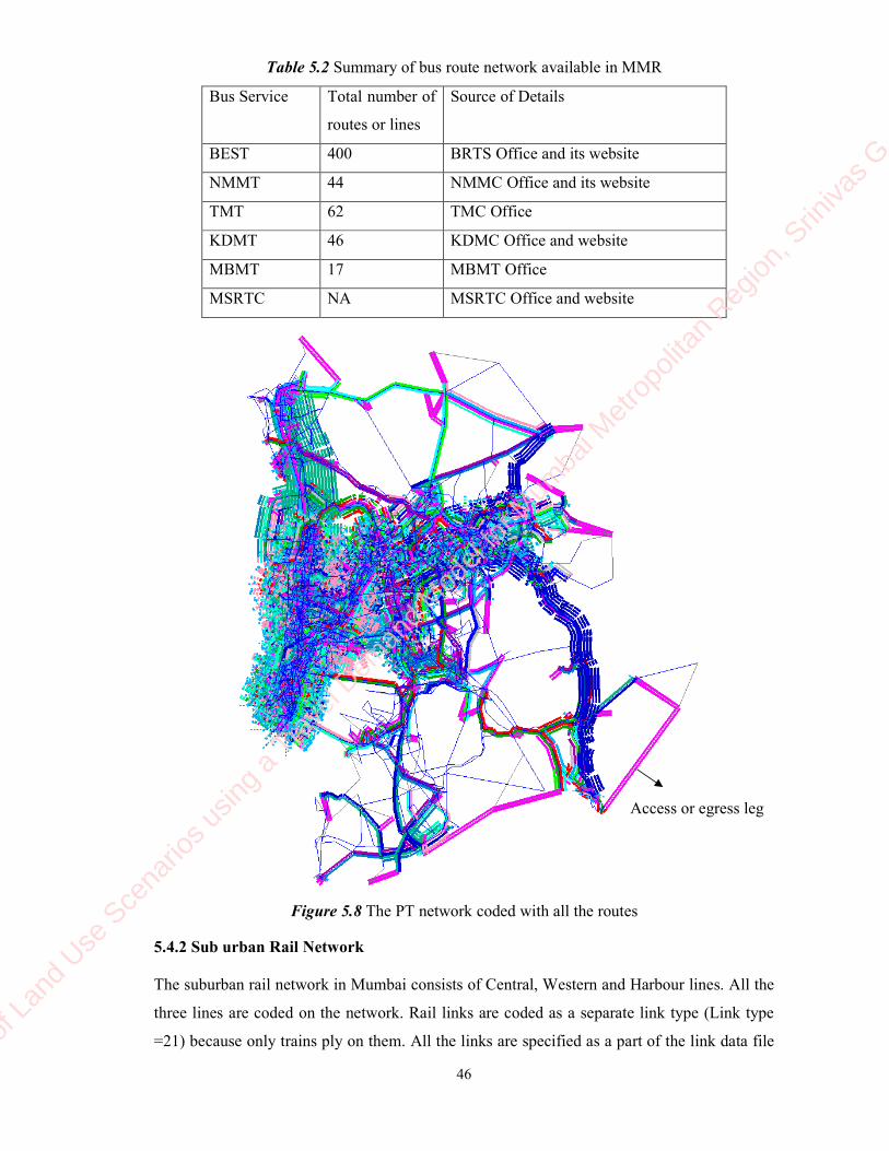
46
Table 5.2 Summary of bus route network available in MMR
Bus Service Total number of
routes or lines
Source of Details
BEST 400 BRTS Office and its website
NMMT 44 NMMC Office and its website
TMT 62 TMC Office
KDMT 46 KDMC Office and website
MBMT 17 MBMT Office
MSRTC NA MSRTC Office and website
Figure 5.8 The PT network coded with all the routes
5.4.2 Sub urban Rail Network
The suburban rail network in Mumbai consists of Central, Western and Harbour lines. All the
three lines are coded on the network. Rail links are coded as a separate link type (Link type
=21) because only trains ply on them. All the links are specified as a part of the link data file
Access or egress leg
Evalua
tion o
f Lan
d Use
Sce
nario
s usin
g a Trav
el Dem
and M
odel
for M
umba
i Metr
opoli
tan R
egion
, Srin
ivas G
, IIT B
omba
y
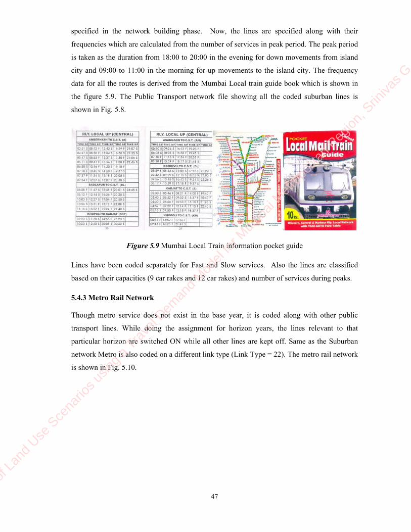
47
specified in the network building phase. Now, the lines are specified along with their
frequencies which are calculated from the number of services in peak period. The peak period
is taken as the duration from 18:00 to 20:00 in the evening for down movements from island
city and 09:00 to 11:00 in the morning for up movements to the island city. The frequency
data for all the routes is derived from the Mumbai Local train guide book which is shown in
the figure 5.9. The Public Transport network file showing all the coded suburban lines is
shown in Fig. 5.8.
Figure 5.9 Mumbai Local Train information pocket guide
Lines have been coded separately for Fast and Slow services. Also the lines are classified
based on their capacities (9 car rakes and 12 car rakes) and number of services during peaks.
5.4.3 Metro Rail Network
Though metro service does not exist in the base year, it is coded along with other public
transport lines. While doing the assignment for horizon years, the lines relevant to that
particular horizon are switched ON while all other lines are kept off. Same as the Suburban
network Metro is also coded on a different link type (Link Type = 22). The metro rail network
is shown in Fig. 5.10.
Evalua
tion o
f Lan
d Use
Sce
nario
s usin
g a Trav
el Dem
and M
odel
for M
umba
i Metr
opoli
tan R
egion
, Srin
ivas G
, IIT B
omba
y
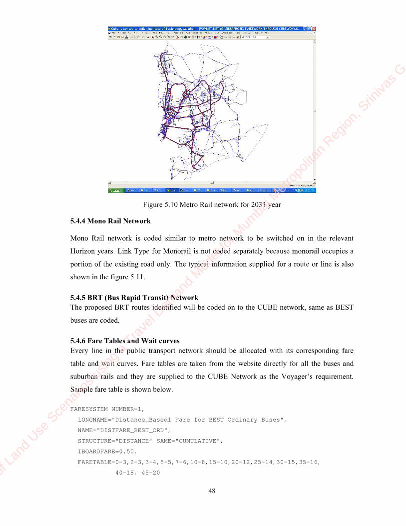
48
Figure 5.10 Metro Rail network for 2031 year
5.4.4 Mono Rail Network
Mono Rail network is coded similar to metro network to be switched on in the relevant
Horizon years. Link Type for Monorail is not coded separately because monorail occupies a
portion of the existing road only. The typical information supplied for a route or line is also
shown in the figure 5.11.
5.4.5 BRT (Bus Rapid Transit) Network
The proposed BRT routes identified will be coded on to the CUBE network, same as BEST
buses are coded.
5.4.6 Fare Tables and Wait curves
Every line in the public transport network should be allocated with its corresponding fare
table and wait curves. Fare tables are taken from the website directly for all the buses and
suburban rails and they are supplied to the CUBE Network as the Voyager’s requirement.
Sample fare table is shown below.
FARESYSTEM NUMBER=1,
LONGNAME="Distance_Based1 Fare for BEST Ordinary Buses",
NAME="DISTFARE_BEST_ORD",
STRUCTURE="DISTANCE” SAME="CUMULATIVE",
IBOARDFARE=0.50,
FARETABLE=0-3,2-3,3-4,5-5,7-6,10-8,15-10,20-12,25 -14,30-15,35-16,
40-18, 45-20
Evalua
tion o
f Lan
d Use
Sce
nario
s usin
g a Trav
el Dem
and M
odel
for M
umba
i Metr
opoli
tan R
egion
, Srin
ivas G
, IIT B
omba
y

49
Figure 5.11 Attributes of a typical Public transport route in CUBE
The wait curves and crowd curves are defined in the same programme of PUBLIC
TRANSPORT in CUBE Voyager. The sample wait curve definition is as follows,
;DEFINITION OF WAIT CURVES WAITCRVDEF NUMBER=1 LONGNAME="InitialWait" NAME="In itWait" , CURVE=1-0.5,16-8,27-12,48-15, 160-20 WAITCRVDEF NUMBER=2 LONGNAME="TransferWait" NAME="X ferWait" , CURVE=1-0.5,4-2,12-6,20-8, 40-15,60-20 CROWDCRVDEF NUMBER=1 NAME="For Buses", CURVE=0-1.43,54-1.65,95-1.87,100-3.74
5.4.7 Creation of Access/Egress and Transfer links
Access or egress legs are the collection of one or more links from the zone centriod to the
nearer transit stop. Access/Egress and transfer links are created using the scripting language
(similar to syntax of C Language), to facilitate the access to the zones and transfer between
the different public transport services. Limiting radius for generating these Non transit legs is
given for each mode differently.
Evalua
tion o
f Lan
d Use
Sce
nario
s usin
g a Trav
el Dem
and M
odel
for M
umba
i Metr
opoli
tan R
egion
, Srin
ivas G
, IIT B
omba
y

50
5.5 Generation of Initial Highway and Public Transport Skims
After building both the highway and public transport network, the highway network is utilized
to generate the initial free flow travel time and distance skims to be given as input to the
demand stage i.e. for trip distribution stage. With the generated connectors for a transit line in
the PT network, the route-enumeration process enumerates routes for each origin zone
connecting to the line via a valid access leg with respect to the factors or parameters given
below. The process is implemented by specifying the appropriate script and input files for
each programme and those programmes used for this step in CUBE are shown in the figure
5.12.
Figure 5.12 Generation of initial highway and PT skims in CUBE voyager platform
1. Maximum number of transfers for a route
MAXFERS=3
2. Number of transfers at which the program stops exploration of less direct routes.
EXTRAXFERS1 = 2
3. Maximum number of transfers explored in excess of the number of transfers required
by the minimum-cost route.
EXTRAXFERS2 = 1
4. SPREAD defines an upper cost limit for routes between an O-D pair.
SPREADFUNC=1, SPREADFACT = 1.05
As shown in the figure 5.12, the enumerated routes are used for the route evaluation in which
the cost of the best route is skimmed based on their probability of use. Then the skim matrices
Evalua
tion o
f Lan
d Use
Sce
nario
s usin
g a Trav
el Dem
and M
odel
for M
umba
i Metr
opoli
tan R
egion
, Srin
ivas G
, IIT B
omba
y

51
are generated which are required for the computation of utility functions in the Modal split
step. The generated skim matrices are listed below.
IVTT_Train - In Vehicle Travel Time by Train
IVTT_Bus - In Vehicle Travel Time by Bus
IVTT_IPT - In Vehicle Travel Time by IPT
IVTT_PV - In Vehicle Travel Time by either Car or TW both of which is same
IVTC_Train - In Vehicle Travel Cost by Train
IVTC_Bus - In Vehicle Travel Cost by Bus
TROVDI - Out of vehicle distance traveled in case of train (access + egress)
BOVDI - Out of vehicle distance traveled in case of bus (access + egress)
5.6 Trip Generation
The trip generation model is the first of the four models of the four step travel demand
modelling process. The trip generation model estimates the number of trips produced and
attracted to each of the TAZ. The trip end models developed during TRANSFORM Study
(2005) for Mumbai Metropolitan Region are adopted here. The trips produced are estimated
from the household socio-economic and trip making characteristics. The trip attractions are
estimated from type of employment categorized in each zone.
Trip end models are classified by six purposes namely,
1. Home Based Work-Office (HBWF)
2. Home Based Work-Industries (HBWI)
3. Home Based Work-Other (HBWO)
4. Home Based Education (HBE)
5. Home Based Other (HBO)
6. Non Home Based (NHB)
Trip End Model excluding walk trips captures the intra study area trips (i.e.) internal to
internal (I-I) made by the residents of the study area for morning peak i.e. 6 a.m to 11 a.m.
Multiple Regression technique was adopted to develop these models. The models adopted for
trip production and trip attraction are shown in table 5.3 and table 5.4.
Table 5.3 Trip Production Model (excluding walk) for various purposes during morning peak
(TRANSFORM, 2005)
Purpose Model R2 t SEE F
HBWF-AM =0.743 RWF 0.90 38.10 4815 1452
Evalua
tion o
f Lan
d Use
Sce
nario
s usin
g a Trav
el Dem
and M
odel
for M
umba
i Metr
opoli
tan R
egion
, Srin
ivas G
, IIT B
omba
y

52
Purpose Model R2 t SEE F
HBWI-AM =0.420 RWI 0.81 26.66 2857 711
HBWO-AM =0.286 RWO 0.85 30.49 3907 929
HBE-AM =0.153 RS 0.81 26.85 3312 721
HBO-AM =0.014 PoP 0.69 19.57 1574 383
NHB-AM =0.002 EBZ 0.19 6.26 297.8 39
Where,
POP : Population
RWF : Resident Worker – Office category
RWI : Resident Worker – Industry category
RWO : Resident Worker – Other category
RS : Resident Student
EBZ : Employment by Zone
HBWF-AM : Home based work-office trip generation during AM peak period
HBWI-AM : Home based work-industry trip generation during AM peak period
HBWO-AM : Home based work-other trip generation during AM peak period
HBE-AM : Home based education trip generation during AM peak period
HBO-AM : Home based other trip generation during AM peak period
NHB-AM : Non-home based all purpose trip generation during AM peak period
The models are statistically significant except the Non home based trips. This is
because of the fact that, it was not possible to capture the NHB trips through any of the
standard socio-economic variables. Since, the percentage of NHB trips in total trips is
marginal (0.39%) and their estimation may not cause significant errors in the network flows.
Table 5.4 Trip Attraction Model (excluding walk) for various purposes during morning peak
(TRANSFORM, 2005)
Purpose Model R2 t SEE F
HBWF-AM =0.742 OJ 0.94 52.27 4999 2838
HBWI-AM =0.477 IJ 0.90 39.16 2363 1535
HBWO-AM =0.293 OtJ 0.88 35.67 3526 1272.8
HBE-AM =0.212 OtJ 0.71 20.58 4429 423
HBO-AM =0.006 Pop + 0.019 EBZ 0.72 5.30, 7.56 1371 215.5
NHB-AM =0.002TJ 0.23 7.19 287.7 51.7
Where,
OJ : Office Jobs/Employment by zone
IJ : Industry Jobs/Employment by zone
OtJ : Other Jobs/Employment by zone
Evalua
tion o
f Lan
d Use
Sce
nario
s usin
g a Trav
el Dem
and M
odel
for M
umba
i Metr
opoli
tan R
egion
, Srin
ivas G
, IIT B
omba
y

53
TJ : Total Jobs/Employment by zone
Pop : Population by zone
EBZ : Employment by Zone
HBWF-AM : Home based work-office trip attraction during AM peak period
HBWI-AM : Home base work-industry trip attraction during AM peak period
HBWO-AM : Home base work-other trip attraction during AM peak period
HBE-AM : Home base education trip attraction during AM peak period
HBO-AM : Home base other trip attraction during AM peak period
HBWF-AM : Home base work-office trip attraction during AM peak period
By using these regression models and the data set of required planning variables the trip
productions and attractions are computed using the GENERATION programme of the CUBE
Voyager for all the purposes by coding the appropriate script. The programme structure is
shown in the figure 5.13.
Figure 5.13 Implementation of Trip Generation, Distribution and Modal split step in Voyager
Evalua
tion o
f Lan
d Use
Sce
nario
s usin
g a Trav
el Dem
and M
odel
for M
umba
i Metr
opoli
tan R
egion
, Srin
ivas G
, IIT B
omba
y
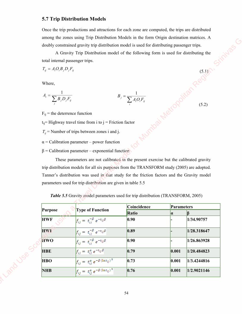
54
5.7 Trip Distribution Models
Once the trip productions and attractions for each zone are computed, the trips are distributed
among the zones using Trip Distribution Models in the form Origin destination matrices. A
doubly constrained gravity trip distribution model is used for distributing passenger trips.
A Gravity Trip Distribution model of the following form is used for distributing the
total internal passenger trips.
ijjjiiij FDBOAT = (5.1)
Where,
∑=
j
ijjj
iFDB
A1
∑
=
i
ijii
jFOA
B1
(5.2)
Fij = the deterrence function
tij= Highway travel time from i to j = Friction factor
ijT = Number of trips between zones i and j.
α = Calibration parameter – power function
β = Calibration parameter – exponential function
These parameters are not calibrated in the present exercise but the calibrated gravity
trip distribution models for all six purposes from the TRANSFORM study (2005) are adopted.
Tanner’s distribution was used in that study for the friction factors and the Gravity model
parameters used for trip distribution are given in table 5.5
Table 5.5 Gravity model parameters used for trip distribution (TRANSFORM, 2005)
Purpose Type of Function Coincidence Parameters
Ratio α β
HWF
0.90 - 1/34.90757
HWI
0.89 - 1/28.318647
HWO
0.90 - 1/26.863928
HBE
0.79 0.001 1/20.484823
HBO
0.73 0.001 1/3.4244816
NHB
0.76 0.001 1/2.9021146
Evalua
tion o
f Lan
d Use
Sce
nario
s usin
g a Trav
el Dem
and M
odel
for M
umba
i Metr
opoli
tan R
egion
, Srin
ivas G
, IIT B
omba
y

55
The productions and attraction for each zone are supplied as inputs and the script for the
gravity model calculations are coded as required for the DISTRIBUTION programme in
Voyager to implement the trip distribution as shown in the figure 5.12. The output of the
programme i.e PA matrix for each purpose is then supplied to the modal split step for the
corresponding purpose.
5.8 Modal Split Models
For this study a simple Multi-Nomial Logit (MNL) mode choice models for morning peak
period without walk trips are used from TRANSFROM study. Table 6.6 lists all the mode
choice models used for the MMR. The total trips from the distribution step are are divided
into captive riders (70% - PT) and choice riders (30%) first for each purpose. The MNL
applied for the choice riders is shown in the figure 5.14. Then the modal split equations are
applied for those choice riders separately for Island and non-Island city.
MNL Model, Island City, Vehicle Available MNL Model, Non-Island, Vehicle Available
Figure 5.14 Summary of Mode Choice Model Structures: Without Walk (TRANSFORM,
2005)
Then the PT users from the choice riders are accumulated and added to the captive
riders. Hence the whole trips are here being divided into PT and PV trips. The adopted Mode
Choice Models for MMR are shown in the table 5.6.
Table 5.6 Proposed Mode Choice Models for GMR (Morning Peak without Walk)
(TRANSFORM, 2005)
Model Availability
of Vehicle
Locat
ion
Rho
Square Utility Equations
HBW-
Employed
in Office
Vehicle
Available
Island
City
0.33
U (Train) = -0.0553*IVTTTrain-0.0192*IVTCTrain-0.485*TROVDI
U (Bus) = 0.08-0.0553*IVTTBus-0.0192*IVTCBus-0.485*BOVDI
U (IPT) = -4.621-0.0553*IVTTTaxi-Rickshaw-0.0192*IPTCOST
U (PVT) = 3.458-0.0553*IVTTCar-TW-0.0192*PVTCOST
U (Metro) = 0.900-0.0553*IVTTmet-0.0192*metCOST-0.97*MOVDI
Non-
Island
0.41 U (Train) = -0.0252*IVTTTrain-0.0148*IVTCTrain-0.1255*TROVDI
U (Bus) = -1.100-0.0252*IVTTBus-0.0148*IVTCBus-0.1255*BOVDI
U (IPT) = -3.8619-0.0252*IVTTTaxi-Rickshaw-0.0148*IPTCOST
U (PVT) = 3.699-0.0252*IVTTCar-TW-0.0148*PVTCOST
U(Metro) = 0.600-0.0252*IVTTmet-TW-0.0148*metCOST-0.251*MOVDI
HBW-
Employed
Vehicle
Available
Island
City
0.44 U (Train) = -0.0506*IVTTTrain-0.0269*IVTCTrain-0.3521*TROVDI
U (Bus) = -0.51-0.0506*IVTTBus-0.0269*IVTCBus-0.3521*BOVDI
Evalua
tion o
f Lan
d Use
Sce
nario
s usin
g a Trav
el Dem
and M
odel
for M
umba
i Metr
opoli
tan R
egion
, Srin
ivas G
, IIT B
omba
y

56
Model Availability
of Vehicle
Locat
ion
Rho
Square Utility Equations
in Industry U (IPT) = -40.353-0.0506*IVTTTaxi-Rickshaw-0.0269*IPTCOST
U (PVT) = 4.0775-0.0506*IVTTCar-TW-0.0269*PVTCOST
U (Met) = 1.00-0.0506*IVTTmet-0.0269*metCOST-.7042*MOVDI
Non-
Island
0.37 U (Train) = -0.0208*IVTTTrain-0.0150*IVTCTrain-0.1354*TROVDI
U (Bus) = -0.63-0.0208*IVTTBus-0.0150*IVTCBus-0.1354*BOVDI
U (IPT) = -3.5727-0.0208*IVTTTaxi-Rickshaw-0.0150*IPTCOST
U (PVT) = 3.987-0.0208*IVTTCar-TW-0.0150*PVTCOST
U (Met) = 0.900-0.0208*IVTTmet-0.0150*metCOST-.2708*MOVDI
HBW-
Employed
in Others
Vehicle
Available
Island
City
0.48 U (Train) = -0.0626*IVTTTrain-0.0254*IVTCTrain-0.126*TROVDI
U (Bus) = 1.04-0.0626*IVTTBus-0.0254*IVTCBus-0.126*BOVDI
U (IPT) = 0.0001-0.0626*IVTTTaxi-Rickshaw-0.0254*IPTCOST
U (PVT) = 2.0647-0.0626*IVTTCar-TW-0.0254*PVTCOST
U (Met) = 2.512-0.0626*IVTTmet-0.0254*metCOST-0.252*MOVDI
Non-
Island
0.50 U (Train) = -0.0325*IVTTTrain-0.0169*IVTCTrain-0.1571*TROVDI
U (Bus) = -1.34-0.0325*IVTTBus-0.0169*IVTCBus-0.1571*BOVDI
U (IPT) = 0.0001-0.0325*IVTTTaxi-Rickshaw-0.0169*IPTCOST
U (PVT) = 4.378-0.0325*IVTTCar-TW-0.0169*PVTCOST
U (Met) = 1.178-0.0325*IVTTmet-0.0169*metCOST-0.3142*MOVDI
HBE Vehicle
Available
Island
City
0.38 U (Train) = -0.0733*IVTTTrain-0.0256*IVTCTrain-0.8412*TROVDI
U (Bus) = 1.400-0.0733*IVTTBus-0.0256*IVTCBus-0.8412*BOVDI
U (IPT) = -4.369-0.0733*IVTTTaxi-Rickshaw-0.0256*IPTCOST
U (PVT) = 1.529-0.0733*IVTTCar-TW-0.0256*PVTCOST
U (Met) = 0.029-0.0733*IVTTmet-TW-0.0256*metCOST-
1.6824*MOVDI
Non-
Island
0.14 U (Train) = -0.0349*IVTTTrain-0.0160*IVTCTrain-0.1737*TROVDI
U (Bus) = 0.45-0.0349*IVTTBus-0.0160*IVTCBus-0.1737*BOVDI
U (IPT) = 2.029-0.0349*IVTTTaxi-Rickshaw-0.0160*IPTCOST
U (PVT) = -0.001-0.0349*IVTTCar-TW-0.0160*PVTCOST
U (Met) = -0.516-0.0349*IVTTmet-0.0160*metCOST-.3474*MOVDI
HBO Vehicle
Available
Island
City
0.16 U (Train) = -0.0405*IVTTTrain-0.0170*IVTCTrain-0.272*TROVDI
U (Bus) = 0.24-0.0405*IVTTBus-0.0170*IVTCBus-0.272*BOVDI
U (IPT) = 0.00012-0.0405*IVTTTaxi-Rickshaw--0.0170*IPTCOST
U (PVT) = 2.7592-0.0405*IVTTCar-TW-0.0170*PVTCOST
U (Met) = 1.459-0.0405*IVTTmet-0.0170*metCOST-0.544*MOVDI
Non-
Island
0.28 U (Train) = -0.0221*IVTTTrain-0.0130*IVTCTrain-0.1760*TROVDI
U (Bus) = -0.6200-0.0221*IVTTBus-0.0130*IVTCBus-0.1760*BOVDI
U (IPT) = 0.00012-0.0221*IVTTTaxi-Rickshaw-0.0130*IPTCOST
U (PVT) = 2.8720-0.0221*IVTTCar-TW-0.0130*PVTCOST
U (Met) = 1.000-0.0221*IVTTmet-0.0130*metCOST-0.352*MOVDI
NHB Vehicle
Available
Island
City
0.16 U (Train) = -0.0405*IVTTTrain-0.0170*IVTCTrain-0.272*TROVDI
U (Bus) = 0.24-0.0405*IVTTBus-0.0170*IVTCBus-0.272*BOVDI
U (IPT) = 0.01-0.0405*IVTTTaxi-Rickshaw--0.0170*IPTCOST
U (PVT) = 3.7592-0.0405*IVTTCar-TW-0.0170*PVTCOST
U (Met) = 1.459-0.0405*IVTTmet-0.0170*metCOST-0.544*MOVDI
Non-
Island
0.28 U (Train) = -0.0221*IVTTTrain-0.0130*IVTCTrain-0.1760*TROVDI
U (Bus) = -0.6200-0.0221*IVTTBus-0.0130*IVTCBus-0.1760*BOVDI
U (IPT) = 0.01-0.0221*IVTTTaxi-Rickshaw-0.0130*IPTCOST
U (PVT) = 3.8720-0.0221*IVTTCar-TW-0.0130*PVTCOST
U (Met) = 1.000-0.0221*IVTTmet-0.0130*metCOST-0.352*MOVDI
Where,
IVTTTrain - In Vehicle Travel Time by Train
IVTTBus - In Vehicle Travel Time by Bus
Evalua
tion o
f Lan
d Use
Sce
nario
s usin
g a Trav
el Dem
and M
odel
for M
umba
i Metr
opoli
tan R
egion
, Srin
ivas G
, IIT B
omba
y
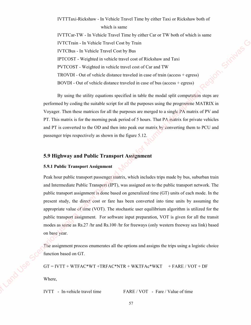
57
IVTTTaxi-Rickshaw - In Vehicle Travel Time by either Taxi or Rickshaw both of
which is same
IVTTCar-TW - In Vehicle Travel Time by either Car or TW both of which is same
IVTCTrain - In Vehicle Travel Cost by Train
IVTCBus - In Vehicle Travel Cost by Bus
IPTCOST - Weighted in vehicle travel cost of Rickshaw and Taxi
PVTCOST - Weighted in vehicle travel cost of Car and TW
TROVDI - Out of vehicle distance traveled in case of train (access + egress)
BOVDI - Out of vehicle distance traveled in case of bus (access + egress)
By using the utility equations specified in table the modal split computation steps are
performed by coding the suitable script for all the purposes using the programme MATRIX in
Voyager. Then these matrices for all the purposes are merged to a single PA matrix of PV and
PT. This matrix is for the morning peak period of 5 hours. That PA matrix for private vehicles
and PT is converted to the OD and then into peak our matrix by converting them to PCU and
passenger trips respectively as shown in the figure 5.12.
5.9 Highway and Public Transport Assignment
5.9.1 Public Transport Assignment
Peak hour public transport passenger matrix, which includes trips made by bus, suburban train
and Intermediate Public Transport (IPT), was assigned on to the public transport network. The
public transport assignment is done based on generalized time (GT) units of each mode. In the
present study, the direct cost or fare has been converted into time units by assuming the
appropriate value of time (VOT). The stochastic user equilibrium algorithm is utilized for the
public transport assignment. For software input preparation, VOT is given for all the transit
modes as same as Rs.27 /hr and Rs.100 /hr for freeways (only western freeway sea link) based
on base year.
The assignment process enumerates all the options and assigns the trips using a logistic choice
function based on GT.
GT = IVTT + WTFAC*WT +TRFAC*NTR + WKTFAc*WKT + FARE / VOT + DF
Where,
IVTT - In-vehicle travel time FARE / VOT - Fare / Value of time
Evalua
tion o
f Lan
d Use
Sce
nario
s usin
g a Trav
el Dem
and M
odel
for M
umba
i Metr
opoli
tan R
egion
, Srin
ivas G
, IIT B
omba
y

58
WT - Waiting time NTR - Number of Transfers
WKT - Walk time DF - Discomfort
Discomfort is taken care by defining different multiple crowding curves for different PT
modes
The initially prepared public transport network and peak hour passenger trip matrix
which is obtained from the Modal split step are given as the input to the PUBLIC
TRANSPORT programme and necessary script is coded implement the public transport
assignment. Then the matrix manipulations have been performed on the loaded PT network
to make it preloaded and then it is given as input to the highway assignment. The loaded
network from the highway assignment is supplied to PT assignment with congested times.
The same procedure is implemented for 3 iterations to stabilize the skims which can be given
input to the modal split step in next iteration.
5.9.2 Highway Assignment
Highway assignment has been carried out for peak hour by preloading the highway network
with peak hour public transport flows in terms of PCUs. A capacity restraint procedure based
on generalized cost was used in loading these PV matrices. Tolls are also considered on the
western freeway sea link. The link type wise parameters for BPR equation for speed flow
relation are taken from the TRANSFORM, 2005 for the calculation of travel cost. These steps
are performed in the script file. The Highway assignment is done based on generalized Cost
(GC)
GC = VOT * TT + TC
Where,
VOT = Value of travel time
TT = Travel time
TC = Travel cost
Parameters of Generalized cost used in Highway Assignment are as below,
VOT = Rs. 80/hr and VOC = Rs. 5/Km
The assignment of PT and Private Vehicle trips were done iteratively till an overall
equilibrium was reached between PT and highway networks. The complete flow structure of
the model developed in CUBE voyager is shown in the figure 5.15 as well as in appendix in
detailed manner.
Evalua
tion o
f Lan
d Use
Sce
nario
s usin
g a Trav
el Dem
and M
odel
for M
umba
i Metr
opoli
tan R
egion
, Srin
ivas G
, IIT B
omba
y

59
Figure 5.15 The complete flow structure of the Travel demand model for MMR in Voyager
5.10 Salient features of the present model
The silent feature of the presently developed model is listed as below.
1. The traditional four step travel model of MMR is implemented for the horizon year
2031 in the Script based CUBE Voyager software for the morning peak hour (09:00 to
10:00) only.
2. All the present and proposed public transport service route data was coded for the
model except a few lines.
3. The gravity model and MNL model are used for the trip distribution and modal slit
respectively for all six purposes.
4. Stochastic User Equilibrium is used for the public transport assignment and capacity
restraint algorithm is implemented for high assignment.
5. The total model is iterated for two times to get the skims stabilized with crowding
conditions
Evalua
tion o
f Lan
d Use
Sce
nario
s usin
g a Trav
el Dem
and M
odel
for M
umba
i Metr
opoli
tan R
egion
, Srin
ivas G
, IIT B
omba
y
60
6. Total running time for the model is about 22 to 24 hours when it is run on a desktop
of 3 GB RAM and with Dual Core processor.
5.11 Summary
This chapter dealt with the development of network as well as the Travel demand model of
horizon year 2031 for evaluation of land use scenarios. Implementation of various steps
involved in the present Travel Demand Model are described in detail and we have adopted the
trip-end, gravity and modal split models of TRANSFORM study for the current study. The
evaluation of urban transportation system performance based on developed model in Voyager
is described in the next chapter.
Evalua
tion o
f Lan
d Use
Sce
nario
s usin
g a Trav
el Dem
and M
odel
for M
umba
i Metr
opoli
tan R
egion
, Srin
ivas G
, IIT B
omba
y

61
Chapter 6
Evaluation of Urban Transportation System’s Performance using
MCDM approach
6.1 General
The travel demand model is run for all the short listed scenarios P2E2, P3E3 and P3E4 and
the results pertaining to the selected indicators are measured from the model and compared
among all the selected scenarios of land use. Then the rating survey results of indicators and
Multiple Criteria decision making analysis which is proposed for the present study are
analyzed in the subsequent sections to choose the best scenario.
6.2 Selected Scenarios
Totally sixteen combinations of scenarios of population and employment were made initially
and then the short-listing from an original sixteen growth scenarios to six scenarios and then
finally to three options was done which are shown in the figure 6.1.
1. P2E2
2. P3E3
3. P3E4
These scenarios are evaluated against the given proposed transportation system for the
horizon year 2031 only. The transportation network is kept same for all the scenarios. The
proposed transportation network includes,
1. The proposed suburban rail network
2. The Metro and Mono network
3. BRTS network
4. The freeways
5. Improvements of major arterials
Evalua
tion o
f Lan
d Use
Sce
nario
s usin
g a Trav
el Dem
and M
odel
for M
umba
i Metr
opoli
tan R
egion
, Srin
ivas G
, IIT B
omba
y

62
Figure 6.1 Overview of Evaluation of Alternative Development Options
(TRANSFORM, 2005)
6.3 Calculation of Selected indicators from the Travel Demand Model
6.3.1 Accessibility to the public transport stops
This is the major thing on which we can decide whether to choose a particular stop or not.
Hence this was studied as the average walking travel time spent to reach a bus stop. It tells us
the accessibility of the public transportation network to all the zones of the study area. Hence
it is considered as a good measure for the proposed transport network. It will also be used for
the planning of the feeder services where the walking to the transit stops are very so that the
PT share will be increased. It is used to evaluate the proposed transportation network by
comparing with the base year network. As this is not sensitive to the land use scenarios, the
results are shown below for the given proposed transportation network.
It can also be quantified as the number of Non-Transit legs generated per zone for the
proposed public transport network. It gives the exposure of the zones to the public transport
within the radius of 1.2 (for buses) to 2 Km (for transit only). The results from the model are
summarized as below.
Total number zones = 1037
Average walking time to a transit stop = 17.2min
Evalua
tion o
f Lan
d Use
Sce
nario
s usin
g a Trav
el Dem
and M
odel
for M
umba
i Metr
opoli
tan R
egion
, Srin
ivas G
, IIT B
omba
y
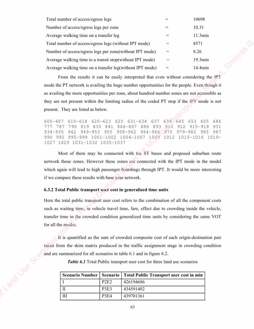
63
Total number of access/egress legs = 10698
Number of access/egress legs per zone = 10.31
Average walking time on a transfer leg = 11.3min
Total number of access/egress legs (without IPT mode) = 8571
Number of access/egress legs per zone(without IPT mode) = 8.26
Average walking time to a transit stop(without IPT mode) = 19.3min
Average walking time on a transfer leg(without IPT mode) = 14.4min
From the results it can be easily interpreted that even without considering the IPT
mode the PT network is availing the huge number opportunities for the people. Even though it
as availing the more opportunities per zone, about hundred number zones are not accessible as
they are not present within the limiting radius of the coded PT stop if the IPT mode is not
present. They are listed as below.
605-607 610-618 620-623 625 631-634 637 639 645 653 655 686 777 787 790 819 835 841 866-867 886 893 910 912 915 -918 931 934-935 942 949-953 955 958-962 964-966 975 979-982 985 987 990 992 995-999 1001-1002 1004-1007 1009 1012 1015- 1016 1019-1027 1029 1031-1032 1035-1037
Most of them may be connected with the ST buses and proposed suburban route
network those zones. However these zones are connected with the IPT mode in the model
which again will lead to high passenger boardings through IPT. It would be more interesting
if we compare these results with base year network.
6.3.2 Total Public transport user cost in generalized time units
Here the total public transport user cost refers to the combination of all the component costs
such as waiting time, in vehicle travel time, fare, effect due to crowding inside the vehicle,
transfer time in the crowded condition generalized time units by considering the same VOT
for all the modes.
It is quantified as the sum of crowded composite cost of each origin-destination pair
taken from the skim matrix produced in the traffic assignment stage in crowding condition
and are summarized for all scenarios in table 6.1 and in figure 6.2.
Table 6.1 Total Public transport user cost for three land use scenarios
Scenario Number Scenario Total Public Transport user cost in min
I P2E2 426194686
II P3E3 434591402
III P3E4 439701361
Evalua
tion o
f Lan
d Use
Sce
nario
s usin
g a Trav
el Dem
and M
odel
for M
umba
i Metr
opoli
tan R
egion
, Srin
ivas G
, IIT B
omba
y

64
Figure 6.2 Total Public transport user cost for three land use scenarios
From the above results, there is no much difference between among the scenarios. But
the P2E2 scenario is leading to the better performance of the proposed transport infrastructure
in this aspect.
6.3.3 Traffic Congestion
Here the traffic congestion is assumed as the percentage of the highway network length which
is being exceeded with the V/C (interpreted as demand/capacity) ratio 1.2. These results are
given in the table 6.2 and figure 6.3 along with the average crowded speed on those highway
network links for all the scenarios.
Percentage of highway network with V/C>1.2 = (length of highway network with V/C>1.2 /
Total length of highway network)*100
Table 6.2 Percentage of highway network with V/C>1.2 for three land use scenarios
Scenario
Number
Scenario Percentage of highway
network with V/C>1.2
Average crowded
speed(Km/hr)
I P2E2 8.80 26.7
II P3E3 10.03 27.7
III P3E4 9.4 28.3
Evalua
tion o
f Lan
d Use
Sce
nario
s usin
g a Trav
el Dem
and M
odel
for M
umba
i Metr
opoli
tan R
egion
, Srin
ivas G
, IIT B
omba
y

65
Figure 6.3 Percentage of highway network with V/C>1.2 for three land use scenarios
6.3.4 Transportation safety
The transportation safety is evaluated with the number of expected fatalities per 10,000 PCU
of private vehicles. Hence the private vehicles PCU’s (peak hour) are taken from the model.
The expected fatality rate is given by Ghee et al, 1997 for developing countries which is
shown in the table 6.3.
Table 6.3 Expected fatality rate for different vehicle ownership level (Ghee et al, 1997) for
developing countries
Vehicle ownership Expected fatality rate
<100 vehicles per 10,000 population 50-100 fatalities per 10,000 PCU
>100 vehicles per 10,000 population 10-50 fatalities per 10,000 PCU
According to the above specifications the expected fatalities are computed for all the
scenarios which are tabulated in the table 6.4. Thirty fatalities per year are assumed, as
vehicle ownership of MMR is more than 100.
Table 6.4 Expected fatalities for MMR in case of all the scenarios
Scenario Number Scenario Private vehicle PCU Expected fatalities
I P2E2 805612 2416
II P3E3 810158 2430
III P3E4 806771 2420
6.3. 5 Mode share of the public transport
The share of the public transport is considered for the peak hour and in that, percentage of the
different public transport modes are also discussed here. The peak hour loadings by all public
transport modes in terms of passenger boardings, passenger distances in Km and passenger
Evalua
tion o
f Lan
d Use
Sce
nario
s usin
g a Trav
el Dem
and M
odel
for M
umba
i Metr
opoli
tan R
egion
, Srin
ivas G
, IIT B
omba
y
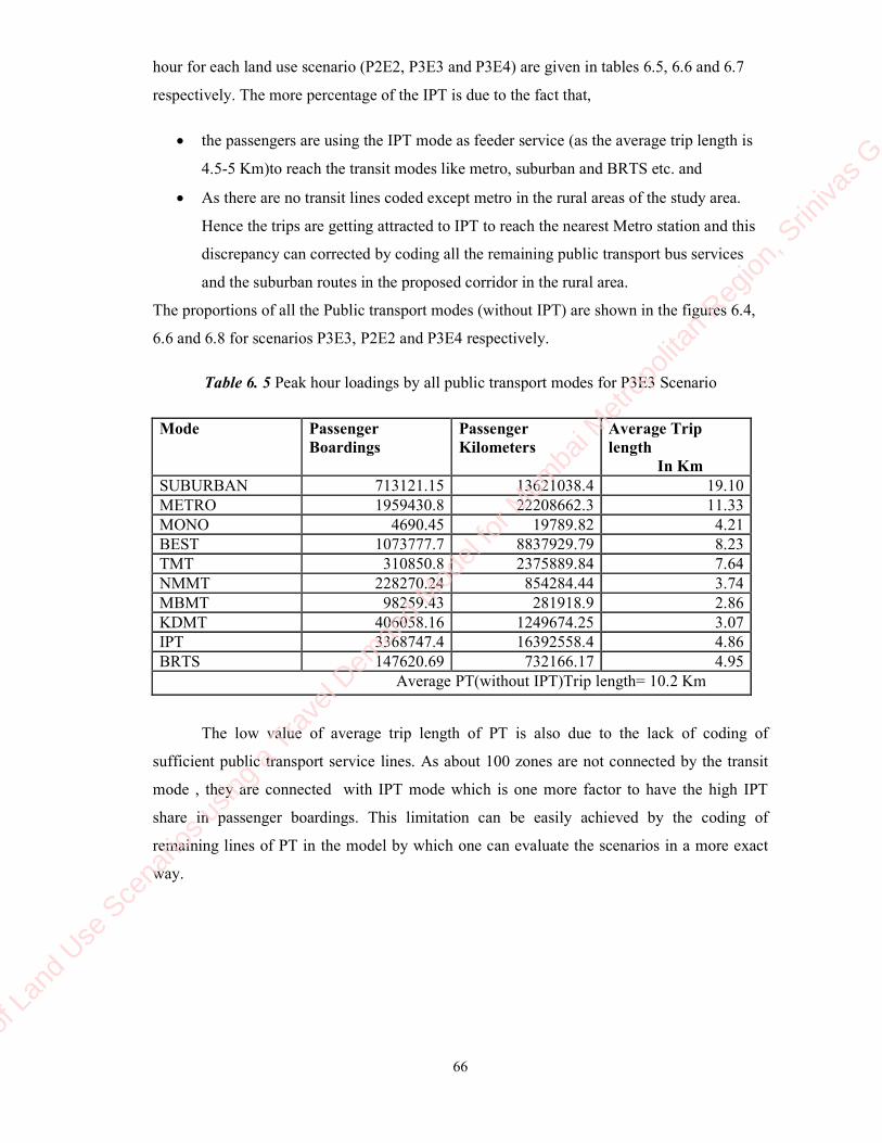
66
hour for each land use scenario (P2E2, P3E3 and P3E4) are given in tables 6.5, 6.6 and 6.7
respectively. The more percentage of the IPT is due to the fact that,
• the passengers are using the IPT mode as feeder service (as the average trip length is
4.5-5 Km)to reach the transit modes like metro, suburban and BRTS etc. and
• As there are no transit lines coded except metro in the rural areas of the study area.
Hence the trips are getting attracted to IPT to reach the nearest Metro station and this
discrepancy can corrected by coding all the remaining public transport bus services
and the suburban routes in the proposed corridor in the rural area.
The proportions of all the Public transport modes (without IPT) are shown in the figures 6.4,
6.6 and 6.8 for scenarios P3E3, P2E2 and P3E4 respectively.
Table 6. 5 Peak hour loadings by all public transport modes for P3E3 Scenario
Mode Passenger
Boardings
Passenger
Kilometers
Average Trip
length
In Km
SUBURBAN 713121.15 13621038.4 19.10
METRO 1959430.8 22208662.3 11.33
MONO 4690.45 19789.82 4.21
BEST 1073777.7 8837929.79 8.23
TMT 310850.8 2375889.84 7.64
NMMT 228270.24 854284.44 3.74
MBMT 98259.43 281918.9 2.86
KDMT 406058.16 1249674.25 3.07
IPT 3368747.4 16392558.4 4.86
BRTS 147620.69 732166.17 4.95
Average PT(without IPT)Trip length= 10.2 Km
The low value of average trip length of PT is also due to the lack of coding of
sufficient public transport service lines. As about 100 zones are not connected by the transit
mode , they are connected with IPT mode which is one more factor to have the high IPT
share in passenger boardings. This limitation can be easily achieved by the coding of
remaining lines of PT in the model by which one can evaluate the scenarios in a more exact
way.
Evalua
tion o
f Lan
d Use
Sce
nario
s usin
g a Trav
el Dem
and M
odel
for M
umba
i Metr
opoli
tan R
egion
, Srin
ivas G
, IIT B
omba
y

67
Figure 6.4 Peak hour PT Modal share for the scenario P3E3 without IPT mode
When we compare the average trip lengths for PT modes, the reasonable values are
coming for the TPT as only 4.5-5 km. The suburban is having the highest the average trip
length in all the scenarios. The average trip lengths in km for PT modes are given in the
figures 6.5, 6.7 and 6.9 for the scenarios P3E3, P2E2 and P3E4 respectively.
Figure 6.5 Peak hour Average trip length of PT modes in Km for the scenario P4E3
Table 6. 6 Peak hour loadings by all public transport modes for P2E2 Scenario
Mode Passenger Boardings Passenger Kilometers Average Trip length
In Km
SUBURBAN 619043.53 12331270.39 19.92
METRO 1772487.86 19870374.94 11.21
MONO 6941.07 31010.1 4.47
BEST 1322137.62 10253645.72 7.76
Evalua
tion o
f Lan
d Use
Sce
nario
s usin
g a Trav
el Dem
and M
odel
for M
umba
i Metr
opoli
tan R
egion
, Srin
ivas G
, IIT B
omba
y

68
Mode Passenger Boardings Passenger Kilometers Average Trip length
In Km
TMT 279477.8 2116294.2 7.57
NMMT 196595.42 793193.22 4.03
MBMT 85942.71 265649.02 3.09
KDMT 1110563.75 27625.33 0.02
IPT 3250024.09 14836433.34 4.57
BRTS 203046.4 1026562.29 5.06
Average PT(without IPT)Trip length= 10.22 Km
Figure 6.6 Peak hour PT Modal share for the scenario P2E2 without IPT mode
Figure 6.7 Peak hour Average trip length of PT modes in Km for the scenario P2E2
Table 6. 7 Peak hour loadings by all public transport modes for P3E4 Scenario
Mode Passenger Boardings Passenger Kilometers Average Trip length
In Km
SUBURBAN 660257.28 11374520.07 17.23
METRO 2173322.53 24343336.74 11.20
MONO 3788.9 14996.72 3.96
BEST 1058345.3 9600520.01 9.07
TMT 336032.06 2443472.46 7.27
NMMT 258083.24 945011.42 3.66
MBMT 94575.3 266417.41 2.82
Evalua
tion o
f Lan
d Use
Sce
nario
s usin
g a Trav
el Dem
and M
odel
for M
umba
i Metr
opoli
tan R
egion
, Srin
ivas G
, IIT B
omba
y

69
Mode Passenger Boardings Passenger Kilometers Average Trip length
In Km
KDMT 463631.2 1440535.52 3.11
IPT 3345553.5 17872938.19 5.34
BRTS 110736.87 529396.09 4.78
Average PT(without IPT)Trip length= 9.8 Km
Figure 6.8 Peak hour PT Modal share for the scenario P3E4 without IPT mode
Figure 6.9 Peak hour Average trip length of PT modes in Km for the scenario P3E4
6.3.6 Average trip length and vehicle kilometers
Average trip length by private vehicles tells us the relative distribution of population or
employment in the study area. The vehicle kilometers by the private vehicles, corresponding
the average trip length and the average speed across scenarios which is varies from 28 to 31
Kmph.is given in the table 6.8.
Evalua
tion o
f Lan
d Use
Sce
nario
s usin
g a Trav
el Dem
and M
odel
for M
umba
i Metr
opoli
tan R
egion
, Srin
ivas G
, IIT B
omba
y

70
Table 6. 8 Vehicle kilometers and Average trip lengths by PV and PT for all the Scenarios
Mode P2E2 P3E3 P3E4
Vehicle kilometers 12721693 13605542 14184850
Average trip length for PV in Km 15.19 16.8 17.5
Average trip length by PT in Km 10.22 10.2 9.8
Average Speed by PV in Kmph 28.65 29.47 30.28
Average Speed by PT in Kmph 29.47 34.64 35.02
6.3.7 Cost of the proposed transportation infrastructure for the Horizon year 2031
This is parameter is same for all the land use scenarios as there is no change considered in the
transport scenario. The cost of the proposed transportation infrastructure according to the
TRANSFORM, 2005 is Rs. 1,887,07 crore which is given in the table 6.9.
Table 6.9 Cost of proposed transport infrastructure for the horizon year 2031
Sl. No. Transport System Length
(kms)
Estimated Total Cost
(Rs. crores)
@ 2005-06 Prices
Estimated
Total Cost
in % of Total
(%)
I Metro System 514 1,158,28 61.4
II Sub-Urban Railway System 241 320,67 17.0
III Highway System 1974 408,12 21.6
Total 2729 1,887,07 100.0
6.4 Analysis of the Rating survey
As proposed in the methodology, the rating survey is done for assigning the relative
weightages to the indicators measured from the model. Totally a twenty number of samples
are taken in which,
Number of samples taken from researchers = 10
Number of samples taken from Common user = 5
Number of samples taken from industrial professional = 5
The corresponding sample survey data sheet is attached in the appendix. Along with
their ratings and rankings for the indicators, their response is also considered according to
which, ITS component is the main indicator on which the public transport service can be
evaluated. However it is assumed here that, the ITS will be functioning well in the horizon
year 2031 for all the scenarios. The summary of average ratings of the three groups of interest
for all the indicators along with their relative weightages are presented in the table 7.9 and
also shown in the figure 7.2.
Evalua
tion o
f Lan
d Use
Sce
nario
s usin
g a Trav
el Dem
and M
odel
for M
umba
i Metr
opoli
tan R
egion
, Srin
ivas G
, IIT B
omba
y

71
6.4.1 Inferences from survey
According to the researchers point of view, the accessibility to the transit modes will be
having the high weightage to evaluate a given transportation system along with the average
trip length through PT. Industrial professionals perceived that the generalized cost through PT
should have a very high importance. A common user perceives that the total cost to the
destination should be low and accessibility to transit mode should be high. Transportation
safety and environmental pollution (here it is indicated according to vehicle kilometers
travelled) is highly preferred to evaluate the transportation system performance.
From the response of the samples, it is inferred that some more indicators can also be
considered while evaluating the transportation system absolutely. They are listed below as,
1. Feeder services performance
2. Passenger travel information system
3. Integration between different transit modes
4. Provision of park and ride facility
5. Provision of non-motorized transport facilities like dedicated bike lanes
6. Pollution cost occurred during construction activity of proposed
transportation infrastructure.
Due to the limitations of the present model these are not considered but they can be
accounted easily for evaluating the absolute transportation system performance.
The selected indicator set for the analysis is listed below,
1. Indicator I – Accessibility to the transit stop
2. Indicator II – Total public transport user cost to the destination
3. Indicator III– Traffic Congestion
4. Indicator IV – Transportation safety
5. Indicator V – Average trip length through PT
6. Indicator VI– Average speed through PT
7. Indicator VII – Vehicle kilometers travelled
8. Indicator VIII – Average trip length through PV
9. Indicator IX – Average speed for PV
Table 6.10 The summary of average ratings of the three groups of interest for all the
indicators
Sl. No Sample type Indicators
I II III IV V VI VII VIII IX
1 Researchers 8.77 8.22 9.11 8 7.22 7.16 6.89 6.89 6.85
2 Common user 7.5 9 8 9 7.5 7.4 7.5 5.5 5.3
Evalua
tion o
f Lan
d Use
Sce
nario
s usin
g a Trav
el Dem
and M
odel
for M
umba
i Metr
opoli
tan R
egion
, Srin
ivas G
, IIT B
omba
y

72
Sl. No Sample type Indicators
I II III IV V VI VII VIII IX
3 Industrial
professional 8 9.5 7 8 6.5 6.35 5.5 4 4
Average rating score 8.46 8.53 8.61 7.84 7.15 7.13 6.76 6.23 6.20
Figure 6.10 The summary of average ratings of the three groups of interest for all the
indicators
6.4.2 Calculation of Relative Transportation performance Index
Relative score is given for all the scenarios based on measure of the each indicator and is
computed as proposed in the methodology.
Relative score of a scenario j with respect to indicator i = 100-(% difference with the best
measure among the scenarios)
Let RWji = Relative weighted score for the scenario j with respect to indicator i
RWji = Relative score of a scenario j * average rating score of that indicator i
Relative Transportation System Performance Index for Scenario j =RTPIj= ∑RWj
The total analysis part is shown in the table 6.11 to arrive at RTPI for each scenario
based on which we can rank them. The same results are also shown in the figure 6.11.
Evalua
tion o
f Lan
d Use
Sce
nario
s usin
g a Trav
el Dem
and M
odel
for M
umba
i Metr
opoli
tan R
egion
, Srin
ivas G
, IIT B
omba
y

73
Figure 6.11 Summary of RTPI for all the scenarios
It is very clear that, all the scenarios are getting differed very less score, however the
scenario P2E2 scenario is the best according to the obtained. The P2E2 tell that inticification
of Greater mumbai in population and employment. This decision is based on the coded Public
transportation network and the inclusion of more sustainable transportation system
performance indicators. Hence this can be modified by overcoming the a few limitations of
the model.
Evalua
tion o
f Lan
d Use
Sce
nario
s usin
g a Trav
el Dem
and M
odel
for M
umba
i Metr
opoli
tan R
egion
, Srin
ivas G
, IIT B
omba
y
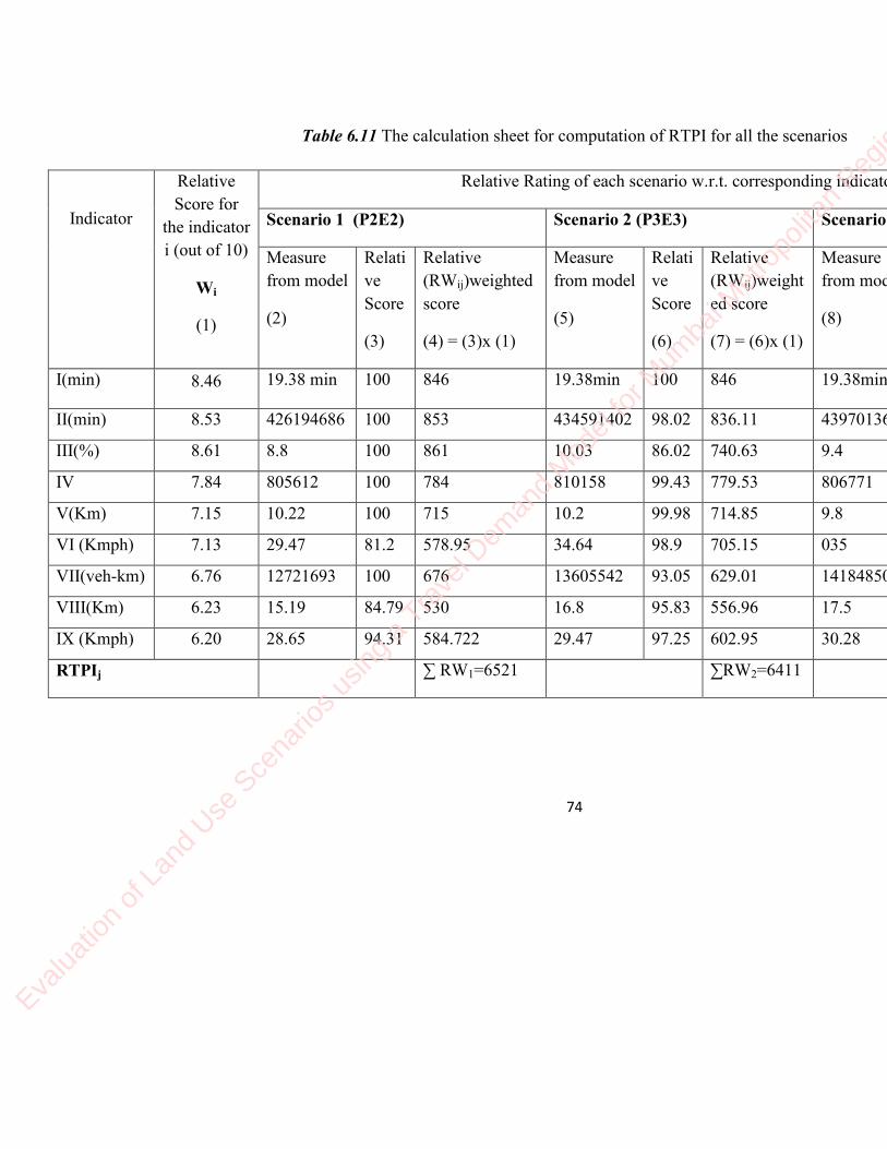
74
Table 6.11 The calculation sheet for computation of RTPI for all the scenarios
Indicator
Relative
Score for
the indicator
i (out of 10)
Wi
(1)
Relative Rating of each scenario w.r.t. corresponding indicator
Scenario 1 (P2E2) Scenario 2 (P3E3) Scenario 3 (P3E4)
Measure
from model
(2)
Relati
ve
Score
(3)
Relative
(RWij)weighted
score
(4) = (3)x (1)
Measure
from model
(5)
Relati
ve
Score
(6)
Relative
(RWij)weight
ed score
(7) = (6)x (1)
Measure
from model
(8)
Relati
ve
Score
(9)
Relative
(RWij)weighted
score
(10) = (9)x (1)
I(min) 8.46 19.38 min 100 846 19.38min 100 846 19.38min 100 846
II(min) 8.53 426194686 100 853 434591402 98.02 836.11 439701361 96.83 825.95
III(%) 8.61 8.8 100 861 10.03 86.02 740.63 9.4 93.18 802.27
IV 7.84 805612 100 784 810158 99.43 779.53 806771 99.8 782.43
V(Km) 7.15 10.22 100 715 10.2 99.98 714.85 9.8 96.0 686.4
VI (Kmph) 7.13 29.47 81.2 578.95 34.64 98.9 705.15 035 100 713
VII(veh-km) 6.76 12721693 100 676 13605542 93.05 629.01 14184850 88.49 598.19
VIII(Km) 6.23 15.19 84.79 530 16.8 95.83 556.96 17.5 100 623
IX (Kmph) 6.20 28.65 94.31 584.722 29.47 97.25 602.95 30.28 100 620
RTPIj ∑ RW1=6521 ∑RW2=6411 ∑ RW3=6402
Evalua
tion o
f Lan
d Use
Sce
nario
s usin
g a Trav
el Dem
and M
odel
for M
umba
i Metr
opoli
tan R
egion
, Srin
ivas G
, IIT B
omba
y

75
Chapter 7
Summary and Conclusions
7.1 Summary of work
The travel is the derived demand of various land use patterns of a region. It can be easily
understood that land means the spatial distribution of locations of various activities in a region
such as residential, commercial, industrial and educational etc., and the transport is the link
between them. Hence the land use determines the magnitude, direction, purpose and spatial
distribution of travel which is to be accommodated by the overall transportation system
present in the region. Either the transportation system should be planned according to the
given land use distribution or the land use distribution should be made for the given
transportation system.
The study has been started with the problem statement of uncertainty in the existing
integrated land use-transport models in the prediction of a transportation system performance.
However even there are no standardized methods to follow to evaluate the given
transportation system. Hence the study has been moved forward with the aim of evaluating
the selected land use scenarios for with respect to the transportation system’s performance.
The study area is taken as the MMR. As the part of the aim the sub-objectives were set as
below.
1. Implementing the travel demand model
2. Selection of transportation performance indicators.
3. Formulation of procedure to evaluate the relative transportation system
performance through MCDM approach.
4. Evaluation of transportation performance using the implemented travel demand
model
In process of implementing the travel demand model, the complete highway and
transit network for horizon year 2031 is developed using the raw shape files got from
MMRDA by incorporating the all the attributes required for the modeling. That complete
network has been developed using the CUBE, TransCAD and ArcGIS tools. Then the
complete route databases of all the public transportation services which can be available in the
year 2031 were coded onto CUBE platform. Then the traditional four step modeling process is
adopted for the travel demand modeling. The demand modeling was done for six purposes for
morning peak hour. The planning variables are taken from MMRDA and modeling process
Evalua
tion o
f Lan
d Use
Sce
nario
s usin
g a Trav
el Dem
and M
odel
for M
umba
i Metr
opoli
tan R
egion
, Srin
ivas G
, IIT B
omba
y

76
was performed using the calibrated models in the TRANSFORM study of MMR conducted in
2005. The trip generation was done based on regression models. The calibrated gravity model
is used for trip distribution. The MNL is utilized in the model split computations. Then the
peak hour matrix of PT and PV are assigned to the network using stochastic user equilibrium
assignment technique and capacity restraint algorithm for public transport and highway
assignment respectively. The whole modeling process was implemented in the CUBE
Voyager software which is a script based transportation planning software.
The literature review has been done to select the indicators which represent the
transportation system performance and some quantifiable indicator set is selected based on the
general guidelines specified in the literature. It has been found from the literature that, there
has been no standard methodology to evaluate the transportation system’s performance.
Hence a procedure is formulated using the MCDM according which a rating survey has been
done to rate the indicators from their own perspectives. The samples are taken from threes
groups of interest such as researchers, industrial professional and common users. After giving
the relative importance to the individual indicators, then those are measured from the travel
demand model for all the selected scenarios P2E2, P3E3 and P3E4 for the given
transportation system for the horizon year 2031. As the part of formulated procedure, the
composite index (RTPI) is computed based on all other indicators. The each scenario is
assigned with the RTPI based on which the best scenario is selected as P2E2.
7.2 Conclusions
There are few conclusions drawn from the review of the literature, implementing the travel
demand model on Voyager software and from the evaluation.
Single level (TAZ level) Traditional four stage travel demand modeling is adopted for
the present study. It is observed from literature review that, the integrated land use
transportation model does not work well for the Indian conditions. Hence the scenario based
approach is adopted for the evaluation of land use scenarios. The various evaluation indices
are reviewed and the indices which represent the environmental, economical and proposed
transportation system based impacts are selected for the present study. As it has been clear
from the literature that, there is no standard criteria for the evaluation an attempt is made to
propose a procedure for the evaluation by considering the response from the researchers,
common user and industrial professionals in a multi criteria decision making approach.
The GIS based network is created for entire MMR covering all the existing and
proposed corridors of all the modes from the shape files along with the preparation of data
base of all the public transport services which is given as input to the travel demand model. It
Evalua
tion o
f Lan
d Use
Sce
nario
s usin
g a Trav
el Dem
and M
odel
for M
umba
i Metr
opoli
tan R
egion
, Srin
ivas G
, IIT B
omba
y

77
is suggested to use more number GIS tools for network building and database management
when we handle such a huge network as there is no single GIS tool which can perform the
entire requirement that we need. It was the largest time taking task performed in the study.
Then the travel demand model is developed for the horizon year 2031 CUBE Voyager
software which was also consumed much time in learning the command language which is
very similar to the basic C language. It has been found that the software provides a very
flexible platform to implement any kind of algorithm to suite our requirement and also
provides the similar GIS platform as in ArcMAP.
The results from the model are discussed which has shown that there is a discrepancy
in the IPT passenger boardings share due to the limitation model which is discussed in the
next section. Without considering the IPT share, in all the scenarios the share for metro is
high w.r.t. passenger boardings but the average trip length for the suburban train is higher.
The rating survey was done to assign the relative importance to each selected indicator, then
the analysis is carried out as proposed in the methodology which led to the decision as P2E2
as the best land use scenario to control growth of the growth scenario. However this decision
can be modified by overcoming the limitations of the model as well as that of the
methodology.
7.3 Limitations
There are certain limitations which are to be considered and corrected to evaluate the
transportation system in a more exact way. They are,
1. Lack of route data coded for the proposed sub-urban rail system for the year 2031 .ST
bus route data is also not coded. A very few of the bus routes of NMMT, BSET and
MBMT bus routes are remaining.
2. The survey was done for only 20 numbers of samples due to the time constraint which
can be increased to more number.
3. The model is developed only for the horizon year 2031 by using the calibrated
parameters from the TRANSFORM study. The hence to the base year model should
also be developed to recalibrate the gravity model, so that forecasts for the 2031 year
can be more reliable.
4. The selected indicators for evaluation represent a few impacts only.
5. Here the only given transportation system is considered for the evaluation i.e. the
evaluation is not done by varying the transport scenarios.
6. The present methodology for evaluation is for computing the relative transportation
performance index only but not the absolute.
Evalua
tion o
f Lan
d Use
Sce
nario
s usin
g a Trav
el Dem
and M
odel
for M
umba
i Metr
opoli
tan R
egion
, Srin
ivas G
, IIT B
omba
y
78
7.4 Future Scope of the work
The future commitments to be completed to achieve the goal for the present study are as
below,
1. Overcoming the limitations stated in the previous section.
2. Performing Sensitivity analysis by considering the relative importance’s of indicators
from each group of interest wise.
3. Conducting a large scale survey to arrive at the more possible set of indicators which
can indicate more impacts for the evaluation and assigning the relative importance
among them.
4. Implementing the methodology for evaluation with tools like Fuzzy logic.
5. Modifying the methodology to compute the absolute transportation system
performance index for the developing countries like India.
Evalua
tion o
f Lan
d Use
Sce
nario
s usin
g a Trav
el Dem
and M
odel
for M
umba
i Metr
opoli
tan R
egion
, Srin
ivas G
, IIT B
omba
y

79
References
Arampatzis, G., Kiranoudis, C., Scaloubacas, P., & Assimacopoulos, D. (2004). “A GIS-
based decision support system for planning urban transportation policies”. European Journal
of Operational Research , Vol. 13(7),pp.465–475.
Baber, C. M., & John, G. (2004). “Baltimore Region Travel Demand Model”. Task Report.
Baltimore Metropolitan Council, Mary land, pp.5-26.
Barra, T. D. (1989). “Integrated land use and transport modeling”. Melbourne, Cambridge
University press, pp.114-120
Beard, D. A. (1993). GIS and Transportation Planning: a case study. Comput. Environ. and
Urban Systems, Vol. 17(3), pp.563-574.
Ghee, C.E, D.T.Silcock, A.Astrop, M.Grove and G.D.Jacobs (1997). “Socio-economic
aspects of road accidents in developing countries”. Transport Research Laboratory.
Crowthorne , pp.25-36.
Gupta, S. (2010). “Urban form-Transport patterns in indian cities and emerging policy
implications”. Sustainable Lifelines: Transportation Planning and Management (pp. 33-39).
Chandigarh: Guru Ramdas School of Planning.
Hwang, C.L. and Yoon, K.P. (1981) “Multiple Attribute Decision Making: Methods and
Applications”, Berlin/Heidelberg/New York: Springer-Verlag, pp. 18-35.
Johnston, R. A., & Clay, M. J. (2005). “Univariate Uncertainty Analysis of an Integrated
Land Use and Transportation Model”. Transportation Planning and Technology,Vol. 28 (5),
pp.149-165.
Littman, T. (2008). “Measuring Transportation Traffic, Mobility and Accessibility”. Victoria
Transport Policy Institute , pp. 1-15.
Littman, T. (2011). “Developing Indicators for comprehensive and Susteainable Transport
Planing”. Victoria Transport Policy Institute , pp. 1-13.
Evalua
tion o
f Lan
d Use
Sce
nario
s usin
g a Trav
el Dem
and M
odel
for M
umba
i Metr
opoli
tan R
egion
, Srin
ivas G
, IIT B
omba
y

80
Moorthy, R., Dhingra, S., & Rao, K.V.K. (2003). “Travel demand assessment in GIS”. Map
Inda, GIS Develpments , pp. 12-20.
Mumbai Metropolitan Region. (2010). Retrieved 10 14, 2010, from Wikipedia:
http://en.wikipedia.org/wiki/Mumbai_Metropolitan_Region
Purvis, C. L. (1997). “Travel Demand Models for the San Francisco Bay Area (BAYCAST-
90)”. Technical Summary .Metropolitan Transportation Commission.,Oakland,
California.,pp. 16-35.
TRANSFORM. (2005). “Comprehensive Transportation study for Mumbai Metropoliatn
region”. Mumbai Metropolitan Region: Lea Associates., 4th
Chapter, Vol. 1 Main Report,
pp.58-230.
Wegener, M., & Furst, F. (1999). “Land-Use Transport Interaction: State of the Art”. Institute
for Raumplanung (Dotumond University), pp.3-23.
Yuan, H, Huapu , L.U., (2003). “Evaluation and analysis of urban transportation efficiency in
China”. Beijing institute of transportation engineering, Tsinghua university, Beijing, china,
pp.2-9.
Zegras, C,(2006). “Sustainable Transport Indicators and assessment methodologies”.
Conference on clean air initiative for latin American cities. Brazil, pp. 1-6.
Evalua
tion o
f Lan
d Use
Sce
nario
s usin
g a Trav
el Dem
and M
odel
for M
umba
i Metr
opoli
tan R
egion
, Srin
ivas G
, IIT B
omba
y

81
Acknowledgments
I am heartily thankful to my supervisor, Prof. K.V. Krishna Rao, whose encouragement,
guidance and support from the initial to the present level enabled me to develop an
understanding and application of the subject to achieve the objective of the study. It is a
pleasure to thank Prof. S.L.Dhingra, who has spent his lot of valuable time to share his
suggestions towards the objective. I also obliged to Prof. Tom V. Mathew, Dr. Gopal Patil,
and Dr. P. Vedagiri for their constant encouragement. I am indebted to all of my classmates,
juniors and friends to support me. I would like to be grateful to the MMRDA organization
which has supplied the required data very timely. I was overwhelmed to CITILABS for their
help in understanding the CUBE Voyager software. Last but not the least, I would like to
thank my seniors Mr. Madhav and Mr. Bala Krishna who were always behind me and
encouraged me in every possible aspect.
Srinivas G
Date:
Place:
Evalua
tion o
f Lan
d Use
Sce
nario
s usin
g a Trav
el Dem
and M
odel
for M
umba
i Metr
opoli
tan R
egion
, Srin
ivas G
, IIT B
omba
y

82
Appendix
Data sheet for Rating and Ranking Survey on Urban Transportation
System Performance Indicators
Name: Income: Age: Date:
Sample Type: Researcher/Industrial/Common User Sample number:
The below indicators are to evaluate the performance of transportation system of a study area.
Please give proper rating and ranking to the indicators based on their dependability to
evaluate the transportation system in your perspective in system level.
If you think an indicator which will be best suited for evaluating the performance, then
you can give rating of maximum 10 and rank 1 then accordingly give the rating for other
indicators.
Indicator
Number
Indicator Rating out 10
marks
Ranking
1 Accessibility to Public Transport(PT) stops from
your home
2 Total Public transport user cost origin to destination
3 Traffic Congestion
4 Transportation safety (number of accidents)
5 Average Trip length through PT
6 Average speed through PT
7 Vehicle kilometers travelled by PV
8 Average Trip length through PV
9 Average speed through PV
Please write if you think there are any other indicators also, to evaluate the urban transportation system performance.
…………………………………….:
…………………………………….:
…………………………………….:
Thank you for your valuable time
Evalua
tion o
f Lan
d Use
Sce
nario
s usin
g a Trav
el Dem
and M
odel
for M
umba
i Metr
opoli
tan R
egion
, Srin
ivas G
, IIT B
omba
y

4 Stage Travel Demand Model Structure implemented in CUBE Voyager
N
E
T
W
O
R
K
D
E
M
A
N
D
S
U
P
P
L
Y
Loop
Iterations=3
Initial Highway and PT costs
Highway and PT costs
Congested Highway and PT
costs
Generation of Initial PT cost
PT Assignment Highway assignment PT/NPT Routes Development
- Loaded PT Network - Loaded PT and PV Network - Congested PT network
- Loading Reports - Loading Reports
- Congested PT Skim - Congested Highway Skim
Loop
Iter =2
Free flow PT network
Congested PT network
PT network
Trip Generation Trip Distribution (Gravity Model) Model Split (MNL)
- Zone wise Productions PA matrix Peak Hour OD Matrix
and Attractions
Zonal Planning Variables
Network Development
(Highway and Public transport)
Public Transport routes Development
and Non Transit leg generation
Generation of Initial Highway Cost
Evalua
tion o
f Lan
d Use
Sce
nario
s usin
g a Trav
el Dem
and M
odel
for M
umba
i Metr
opoli
tan R
egion
, Srin
ivas G
, IIT B
omba
y