Mathematics and Computing/Science/Technology MST326 RB

MST326 Mathematical methods and fluid mechanics

MST326 Revision Booklet

Contents Introduction 2

1 Ordinary differential equations 31.1 Separation of variables 31.2 Integrating factor method 51.3 Which method to use? 61.4 Second-order equations 7

2 Functions of more than one variable 102.1 Partial differentiation 102.2 Taylor polynomials 112.3 The Chain Rule 13

3 Vector algebra and calculus 143.1 Addition, scalar and vector products 143.2 Position, velocity and acceleration 163.3 Gradient of a scalar field 183.4 Divergence and curl of a vector field 19

4 Integration of scalar and vector fields 204.1 Line integrals 204.2 Surface integrals 224.3 Volume integrals 23

5 Dimensions 25 5.1 Dimensional consistency 255.2 Dimensional analysis 27

Solutions to the exercises 29

Index 36

cCopyright © 2009 The Open University WEB 00247 7 1.1

Introduction

The purpose of this Revision Booklet is to remind you of the important techniques which are assumed as background material for the course. You should have met all the material in this booklet in previous courses, so the exercises may be treated as revision. They are designed to give you practice at those techniques for which you might be rusty, and to help you to ‘warm up’ for the course.

This booklet contains no theory or explanation of why the methods for solving particular problems are chosen. However, some references are given below. Each subsection (except 1.3) is divided into three parts: (a) a worked example, showing the procedure to adopt when solving

problems of the type given; (b) a structured exercise for you to attempt, with questions or instructions

to guide you to the answer; (These questions are typical of what you should ask yourself when solving similar problems. They are based on the procedure boxes of MST209. Full solutions to these exercises are given at the back of the booklet.)

(c) one or more further exercises for you to try. (Some of these exercises occur again in Block 1 of the course. Only the answers to these exercises, not full solutions, are given at the back.)

The following table lists the techniques that are revised in this booklet, and where the background theory can be found.

Technique to be revised Section MST209 reference

Ordinary differential equations 1 First-order: Unit 2 Second-order: Unit 3

Functions of more than one variable 2 Unit 12

Vector algebra and calculus 3 Units 4, 23, 24

Integration of scalar and vector fields 4 Units 24, 25

Dimensions 5 Unit 16

If in attempting the further exercises you become stuck, then refer to the appropriate units of the prerequisite course(s) that you studied.

It is best to begin each section by attempting the worked example as an exercise. If you find this difficult, then study the solution to the worked example and attempt the following structured exercise. Otherwise, move on to the further exercises.

The booklet is best worked through before the beginning of the course. However, if you prefer, it is possible to work through different sections during the study of early units, as indicated in the following table.

MST326 Unit Study this material in the Revision Booklet first

1 1.1–1.3: Ordinary differential equations of first order 4.2: Surface integrals

2 1.4: Ordinary differential equations of second order

3 2: Partial differentiation and the Chain Rule

4 3: Vector algebra and calculus 4: Line, surface and volume integrals

6 5: Dimensions

2

1 Ordinar y differential equations

1.1 Separation of variables

Example 1.1

Find the particular solution of the differential equation Each worked example has a solution in two columns, as

dy =

1 explained below. dx ey (1 + x2)

that satisfies the condition y(1) = 0.

Solution

In this column the necessary steps are identified. In this column the calculations are shown.

This differential equation is of first order and non- linear. Separation of variables is applicable because dy

=1 1 ×

1 = the right-hand side can be written as the product dx ey (1 + x2) 1 + x2ey

of a function of y and a function of x.

Divide through by the ‘function of y’ on the right-hand side. Then everything involving y is on the dy

=1

left-hand side of the equation and everything in- ey

dx 1 + xvolving x is on the right-hand side. (In this way,

2

the variables have been separated.) 1

Now integrate both sides of the equation with re- ey dy dx = dx

1 + x2dxspect to x, and apply the rule for integration by 1

2dx

1 + xsubstitution on the left to reach an integral with ey dy = respect to y.

Evaluate the integrals. (You may need to refer to the table of standard integrals given in the Hand­book . Remember to add an arbitrary constant C ey = arctan x + Cwhen integrating the right-hand side.) This givesthe general solution of the differential equation inimplicit form.

Where possible, try to rearrange the solution togive y in terms of x (which is the explicit form of y = ln(arctan x + C)the general solution).

Now use the given condition, y(1) = 0, by putting When x = 1, y = 0, so 0 = ln(arctan 1 + C),1 4π.x = 1 and y = 0 in the general solution. Hence find that is, C = 1 − arctan 1 = 1 −

a value for the constant C.

Substituting the value of C back into the general 1 4πsolution gives the required particular solution. This y = ln arctan x + 1 −

satisfies both the differential equation and the con-dition y(1) = 0.

Comment

Any solution (general or particular) obtained from a differential equation can be checked by substituting it back into the differential equation. A particular solution can also be checked by substituting it into any additional (initial or boundary) conditions that it was intended to satisfy.

3

Exercise 1.1

Obtain the general solution of the differential equation xdy

= e

. dx y

Find also the particular solution that satisfies the condition y(0) = 1.

Steps

(a) Is the differential equation of the type that can be solved by the separation of variables technique?

(b) Rearrange the equation so that all of the terms involving y are on the left-hand side and those involving x are on the right-hand side.

(c) Now integrate both sides and rearrange the solution to give y in terms of x. (This gives the general solution.)

(d) Put x = 0 and y = 1 to find the value of the arbitrary constant. Substitute this value into the general solution. (This gives the particular solution.)

Exercise 1.2

Each worked example is followed by a structured exercise, like this. The steps (questions or instructions) after the problem statement are designed to lead you to the solution of the problem. You can check your solutions against those at the back of the booklet.

Solve the following differential equations and, in each case, find the Each structured exercise is particular solution that satisfies the given condition. followed by one or more further exercises, like this. (a)

dp = −

ρ0g p, p(0) = p0, where p0, ρ0 and g are constants. Answers to these exercises are dz p0 given at the back of the

booklet. xy

(b) dy

= x2 + 1

, y(0) = 5. dx

1(c) dy

= (y + 1) sin x, y π = 0. dx 2

gp(d)

dp = −

R(Θ0 − kz) , p(0) = p0,

dz

where R, g, Θ0, k and p0 are constants.

1(e) y2 dy

= (−2 < x < 2), y(0) = 3. dx (x + 2)(2 − x)

1 1 1 1Hint: = + for − 2 < x < 2.

(x + 2)(2 − x) 4 x + 2 2 − x

4

x

1.2 Integrating factor method

Example 1.2

Find the particular solution of the differential equation

dy = x 2 + 2y (x > 0)

dx that satisfies the condition y(1) = 2.

Solution

This differential equation is of first order, but the variables cannot be separated. It can be solved using the integrating factor method , because it can be written in the form

dy + g(x) y = h(x),

dx where g(x) and h(x) are given functions. This is a linear differential equation.

Divide through by x, so that the coefficient of dy/dx is 1, and bring the y term to the left-hand side. The equation can then be seen to be of the required form.

Identify the two functions g(x) and h(x).

The integrating factor, p(x), is defined by

p(x) = exp g(x) dx .

Multiply the differential equation through by p(x). It can then be written in the form

d [p(x) y] = h(x) p(x), so that

dx p(x) y = h(x) p(x) dx.

Evaluate the integral on the right-hand side, to ob-tain the implicit form of the general solution.

Rearrange to obtain y in terms of x, that is, the explicit form of the general solution.

Now use the given condition y(1) = 2 to find the value of C.

This value gives the required particular solution, which satisfies the differential equation and the con-dition y(1) = 2.

dy x = x2 + 2y

dx

dy 2 − y = x dx x

g(x) = −2/x, h(x) = x.

2

p(x) = exp − dx = exp(−2 ln x) x

−2−2)= exp ln(x = x

1 dy 2 1 − 3 y =

x2 dx x x

d 1 1 2 y =

dx x x

1 1 2 y = dx

x x

1 2 y = ln x + C

x

y = x2(ln x + C) (x > 0)

When x = 1, y = 2, so 2 = C.

y = x2(2 + ln x)

Comment

No constant of integration is needed in the expression for the integrating factor, p(x). Once p(x) has been found, it is good practice to check that

d [p(x) y] = p(x)

dy + p(x) g(x) y.

dx dx

5

Exercise 1.3

Obtain the general solution of the differential equation

dy = x + y.

dx Find also the particular solution that satisfies the condition y(0) = 1.

Steps

(a) Is the differential equation linear? If so, what are g(x) and h(x)?

(b) Find the integrating factor, p(x), for this problem.

(c) Multiply the differential equation through by p(x), and write the left-hand side as a derivative. Integrate both sides, then rearrange the solution to give y in terms of x. (This gives the general solution.)

(d) Put x = 0 and y = 1 to give a value for the arbitrary constant. Substitute this value into the general solution. (This gives the particular solution.)

Exercise 1.4

Solve the following differential equations, and find in each case the particular solution that satisfies the given condition.

(a) xdy

= x3 − 3y (x > 0), y(1) = 1. dx

(b) dy

= sin x + y tan x dx

−1 2π < x < 1

21 y(0) = π , .2

(c) dy − λy = eλx , y(0) = 2, where λ is a constant. dx

(d) (2x + 1) dy

= x − 2y (x > − dx

1 2), y(2) = 0.

(e) dy dx

= y + x2 , y(1) = 5.

1.3 Which method to use? The above two methods of solving first-order differential equations can be used only for certain types of equation. One of the first steps in solving a problem involving a first-order differential equation is to decide whether either method is suitable. The following exercise enables you to revise this important first step. There is no need to solve the equations.

Exercise 1.5

Which of the following equations may be solved by A separation of variables; B the integrating factor method; C neither of the above methods?

(a) dy dx

= x (b) dy dx

= y (c) dy dx

= xy

dy dy = y2 (f)

dydx

= x + y2(d) (e)= x − ydx dx

√(g)

dy = x2 + y (h)

dy = 1 + y (i)

dy =

√ x + y

dx dx dx

6

1.4 Second-order equations

Example 1.3

Find the particular solution of the differential equation

d2y − 2 dy

+ 5y = 2x + 3 dx2 dx

that satisfies the conditions y(0) = 4 and dy

(0) = 1. 5 dx

Solution

The differential equation is of second order, because the order of the highest derivative is 2. It is linear, because the coefficients of y, dy/dx and d2y/dx2

are not functions of y or its derivatives. It is inho­mogeneous , since there are non-zero terms that do not involve y or its derivatives. The coefficients of y and its derivatives are constants, namely, a = 1, b = −2 and c = 5.

For linear inhomogeneous second-order differential equations, the general solution is the sum of the complementary function and a particular integral. First find the complementary function, which is the general solution of the associated homogeneous equation

a d2y dx2

+ b dy dx

+ cy = 0. (1)

A solution of this constant-coefficient equation is of the form eλx . Substitution of eλx into each term of Equation (1) gives a quadratic equation in λ known as the auxiliary equation,

aλ2 + bλ + c = 0, (2)

which needs to be solved for λ.

(i) If Equation (2) has two real roots, λ1 and λ2, then the general solution of Equation (1) is

y(x) = Aeλ1x + Beλ2x ,

where A and B are arbitrary constants. (ii) If Equation (2) has only one real root, λ1 (since

aλ2 + bλ + c is a perfect square), then the gen-eral solution of Equation (1) is

λ1x y(x) = (A + Bx)e .

(iii)If Equation (2) has complex conjugate roots, λ = α + iβ and λ = α − iβ, then the general solution of Equation (1) is

y(x) = e αx(A cos(βx) + B sin(βx)).

Here we have case (iii), with α = 1 and β = 2. (Second-order equations have two arbitrary con-stants in the general solution, here A and B.)

The given (inhomogeneous) differential equation is

d2y − 2 dy

+ 5y = 2x + 3. dx2 dx

The associated homogeneous equation is

d2y − 2 dy

+ 5y = 0. dx2 dx

The auxiliary equation is

λ2 − 2λ + 5 = 0, so √ 2 ± 4 − 20 2 ± 4i

λ = = = 1 ± 2i.2 2

The complementary function is

yc = e x(A cos(2x) + B sin(2x)).

7

A particular integral is any function that satisfies the given inhomogeneous differential equation. The following table shows the usual form of the partic-ular integral, given as a trial (test) function, for some of the different functions f (x) which may ap-pear on the right-hand side of the inhomogeneous differential equation.

f (x) Trial function, yp

m (constant) p (constant) m1x + m0 p1x + p0

mekx pekx

m cos(Ωx) + n sin(Ωx) p cos(Ωx) + q sin(Ωx)

Here there is a linear function of x on the right-hand side, so seek p1 and p0 such that yp = p1x + p0

satisfies the differential equation.

Substitute for yp, dyp/dx and d2yp/dx2 in the dif-ferential equation, to obtain two equations for p1

and p0. The solutions for p1 and p0 give the par-ticular integral for this problem.

The sum of the complementary function and the particular integral is the general solution of the original differential equation.

Now use the two given conditions, y(0) = 4 and5 (dy/dx)(0) = 1, to find values for the constants A and B. For the second condition, the derivative of the general solution is needed.

Substituting the values of A and B back into the general solution gives the required particular solu-tion. This satisfies the differential equation and the two given conditions.

The given inhomogeneous equation is

d2y − 2 dy

+ 5y = 2x + 3. dx2 dx

Try yp = p1x + p0. d2ypThen

dyp = p1 and = 0, so dx dx2

0 − 2p1 + 5(p1x + p0) = 2x + 3,

that is, 5p1x + (5p0 − 2p1) = 2x + 3.

Comparing coefficients gives

5p1 = 2 and 5p0 − 2p1 = 3, so

p1 = 2 and p0 = 19 5 25 .

The particular integral is

yp = 2 x + 19 5 25 .

The general solution is y = yc + yp, that is,

x + 19y = e x(A cos(2x) + B sin(2x)) + 2 5 25 .

4 4 = A + 19 1When x = 0, y = 5 , so 25 , and A = .5 25 The derivative of the general solution is (using the Product Rule)

dy = e x((A + 2B) cos(2x) + (B − 2A) sin(2x)) + 2

dx 5 .

When x = 0, dy/dx = 1, so 71 = A + 2B + 2 = 2B + 11 and B = 25 .5 25

The particular solution is 1 7 + 2 x + 19 y = e x 25 cos(2x) + 25 sin(2x) 5 25 .

Comment

Exceptionally, the ‘trial function’ does not work if the function to be tried contains a term that is a solution of the associated homogeneous equation (1). In this case, multiply the trial function by x (and if that still does not work, multiply the original trial function by x2).

Note that the complementary function, yc, should be found before the particular integral, yp. The additional conditions (at x = 0 in Example 1.3) should be applied to the general solution, y = yc + yp, and not to yc alone.

8

Exercise 1.6

Find the particular solution of the differential equation

2xd2y + 2

dy − 3y = e dx2 dx

that satisfies the conditions y(0) = 1 and dy

(0) = 0. 5 dx Steps

(a) Is the differential equation linear, with constant coefficients and of second order? What is the associated homogeneous equation?

(b) Write down and solve the auxiliary equation. Hence find the complementary function.

(c) Use a ‘trial function’ to find a particular integral that satisfies the given inhomogeneous differential equation.

(d) Add the particular integral to the complementary function, to obtain the general solution.

(e) Put x = 0, y = 1 and x = 0, dy/dx = 0 in turn, to find a value for 5 each of the unknown constants in the general solution. This gives the required particular solution.

Exercise 1.7

Solve the following differential equations and, in each case, find the particular solution for which y = 0 and dy/dx = 1 when x = 0.

−4x(a) 5 d2y − 6

dy + y = 21e

dx2 dx

(b) 5 d2y − 6

dy + y = ex/5

dx2 dxd2y

(c) 4 + y = sin x dx2

(d) d2y − 2

dy + y = 5x − 2

dx2 dxd2y dy

(e) + + y = cos(3x) − 2 sin(3x)dx2 dx

Exercise 1.8

Find the general solution of the differential equation

d2y 3x+ 16y = cos(4x) − 8e . dx2

Find also the particular solution for which y = 0, dy/dx = 0 when x = 0.

9

2 Functions of more than one variable

2.1 Partial differentiation

Example 2.1

Find the second-order partial derivatives of the function Partial derivatives may be denoted using subscripts,

u(x, y) = cos(4x + 3y), with ux for ∂u/∂x,

∂2u ∂2u uxy for ∂2u/∂x ∂y, etc. and confirm that = (or equivalently, uxy = uyx).

∂x ∂y ∂y ∂x

Solution

The first step is to calculate the first-order partial derivatives, ∂u/∂x (i.e. ux) and ∂u/∂y (i.e. uy ).

The first of these, ∂u/∂x, is calculated by differen-tiating u with respect to x while holding y constant. In other words, y is treated as if it were a constant.

Now, to find ∂u/∂y, differentiate u with respect to y while holding x constant. This time, x is treated as a constant.

The second-order partial derivatives are ∂2u/∂x2

(i.e. uxx), ∂2u/∂x ∂y (i.e. uxy ), ∂2u/∂y2 (i.e. uyy ) and ∂2u/∂y ∂x (i.e. uyx). Here ∂2u/∂x2 is obtained by differentiating ∂u/∂x partially with respect to x (treating y as a constant.)

Now ∂2u/∂x ∂y is obtained by differentiating ∂u/∂y partially with respect to x (keeping y con-stant).

For ∂2u/∂y2, differentiate ∂u/∂y partially with re-spect to y (keeping x constant).

Finally, obtain ∂2u/∂y ∂x by differentiating ∂u/∂x partially with respect to y (keeping x constant).

This property of mixed second-order partial deriva-tives is valid for all functions that will be met in the course.

u(x, y) = cos(4x + 3y)

∂u = − sin(4x + 3y) × 4

∂x = −4 sin(4x + 3y)

∂u = − sin(4x + 3y) × 3

∂y = −3 sin(4x + 3y)

∂2u ∂ = (−4 sin(4x + 3y))

∂x2 ∂x= −4 cos(4x + 3y) × 4

= −16 cos(4x + 3y)

∂2u ∂ = (−3 sin(4x + 3y))

∂x ∂y ∂x

= −3 cos(4x + 3y) × 4

= −12 cos(4x + 3y)

∂2u ∂ = (−3 sin(4x + 3y))

∂y2 ∂y = −3 cos(4x + 3y) × 3

= −9 cos(4x + 3y)

∂2u ∂ = (−4 sin(4x + 3y))

∂y ∂x ∂y = −4 cos(4x + 3y) × 3

= −12 cos(4x + 3y)

Comparison with ∂2u/∂x ∂y confirms that

∂2u ∂2u = .

∂x ∂y ∂y ∂x

10

Exercise 2.1

Find the second-order partial derivatives of the function

u(x, y) = A cos(ax) e −a2y , where a and A are constants,

∂2u ∂2uand confirm that = .

∂x ∂y ∂y ∂x

Steps

(a) Differentiate u partially with respect to x (treating y as if it were a constant) to find ∂u/∂x. Now differentiate u partially with respect to y (treating x as if it were a constant) to find ∂u/∂y.

(b) Keeping y constant, differentiate ∂u/∂x with respect to x, to find ∂2u/∂x2 .

Keeping y constant, differentiate ∂u/∂y with respect to x, to find ∂2u/∂x ∂y.

Keeping x constant, differentiate ∂u/∂y with respect to y, to find ∂2u/∂y2 .

Keeping x constant, differentiate ∂u/∂x with respect to y, to find ∂2u/∂y ∂x. Confirm that ∂2u/∂x ∂y = ∂2u/∂y ∂x.

Exercise 2.2

Find the second-order partial derivatives of the following functions.

(a) u(x, y) = sin(x − y)

(b) u(r, θ) = r ln θ (θ > 0)

(c) u(s, t) = sin(st)

Exercise 2.3

(a) Find the first-order partial derivatives ∂u/∂x and ∂u/∂t for −4t u(x, y, z, t) = (x 2 + y 2 + z 2) e .

(b) Find also the second-order partial derivatives ∂2u/∂x ∂y and ∂2u/∂z ∂t.

2.2 Taylor polynomials

Example 2.2

The form of the second-order Taylor polynomial p2(x, y) for a function of two variables u(x, y) about the point (a, b) is

p2(x, y) = u(a, b) + (x − a) ∂u ∂x

(a, b) + (y − b) ∂u ∂y

(a, b) + 1 2(x − a)2 ∂

2u ∂x2

(a, b)

+ (x − a)(y − b) ∂2u

∂x∂y (a, b) + 1

2(y − b)2 ∂2u

∂y2 (a, b).

Find the second-order Taylor polynomial for the function The first- and second-order

u(x, y) = cos(4x + 3y) partial derivatives for this function were obtained in

about the point

1 8π, 1

6π . Example 2.1.

11

Solution

The necessary partial derivatives were obtained previously; now the function and its derivatives

1 1need to be evaluated at π, π .8 6

1 1First evaluate at 8π,6π the function

1 1 6 4 × π6

1+ 3π ×1 8 = cos π = −1u(x, y) = cos(4x + 3y). π, π = cos u 8

1 8π,1

6πNow evaluate at the first-order partial derivatives

∂u ∂u(x, y) = −4 sin(4x + 3y), 1 1 = −4 sin π = 0π, π8 6∂x ∂x

∂u ∂u(x, y) = −3 sin(4x + 3y). 1

81 = −3 sin π = 0π, π6∂y ∂y

Evaluate the second-order partial derivatives

∂2u ∂2u

∂x2 (x, y) = −16 cos(4x + 3y), 1

81 = −16 cos π = 16 π, π6∂x2

∂2u ∂2u 1 1(x, y) = −12 cos(4x + 3y), = −12 cos π = 12 π, π8 6∂x ∂y ∂x ∂y

∂2u ∂2u 1 1

∂y2 (x, y) = −9 cos(4x + 3y).

∂y2

Now substitute these values into the formula

= −9 cos π = 9π, π8 6

The polynomial p2(x, y) is for p2(x, y). −1 + 0

21 8

1 6 +1

2 1 8π+ 0 × 16x − y − x −π π 21 1 1 1+ 12 × 9+x − y − y −π π π8 6 2 62

+ 12 1 8π 1

8π 1 6= −1 + 8 x − x − y − π 2

π9 1+ y − .2 6

Exercise 2.4

Find the second-order Taylor polynomial for the function u(x, y) = sin(xy) 1 4about the point 0, π .

Steps 1 4(a) Find u 0, π .

1 4(b) Use the solution of Exercise 2.2(c) to find (∂u/∂x) 0, π and

1 4(∂u/∂y) 0, π .

(c) Referring to the same solution, calculate the second-order partial 1 4derivatives at 0, π .

(d) Substitute the values for the derivatives found above into the formula This formula is given in the for the second-order Taylor polynomial, and simplify where possible. statement of Example 2.2.

Exercise 2.5

xFind the second-order Taylor polynomial for the function u(x, y) = e cos y about the point (0, 0).

12

2.3 The Chain Rule

Example 2.3

Use the Chain Rule du ∂u dx ∂u dy

= + ds ∂x ds ∂y ds

to find du/ds, where 2 u(x, y) = x 2 +

√ y (y ≥ 0) and x = 2s, y = s .

Solution

First work out all of the derivatives on the right-hand side of the Chain Rule.

Now substitute these derivatives into the formula.

Then substitute for x and y in terms of s.

Notice that substituting for x and y in the expres-sion for u, and then differentiating with respect to s, leads to the same result.

Exercise 2.6

∂u dx= 2x; = 2;

∂x ds ∂u 1= 2y −1/2;

dy = 2s.

∂y ds

du = 2x × 2 + 1

2y −1/2 × 2s = 4x + √ s

ds y

du s= 4 × 2s + √ = 8s + 1

ds s2

√ u = (2s)2 + s2 = 4s 2 + s, so du

= 8s + 1. ds

Use the Chain Rule to find du/ds, where 2 u = x 2 + y and x = cos s, y = sin s.

Steps

(a) Find the derivatives ∂u/∂x, ∂u/∂y, dx/ds, dy/ds.

(b) Substitute into the Chain Rule, as given in Example 2.3.

(c) Substitute for x and y in terms of s.

Exercise 2.7

Use the Chain Rule to find du/ds in each of the following cases.

(a) u(x, y) = x2 − y2 and x = 2s, y = 1 − 2s;

(b) u(x, y) = x2y − xy2 and x = cos s, y = sin s;

(c) u(x, y) = ey cos x and x = s2, y = s3 .

13

3 Vector algebra and calculus

3.1 Addition, scalar and vector products

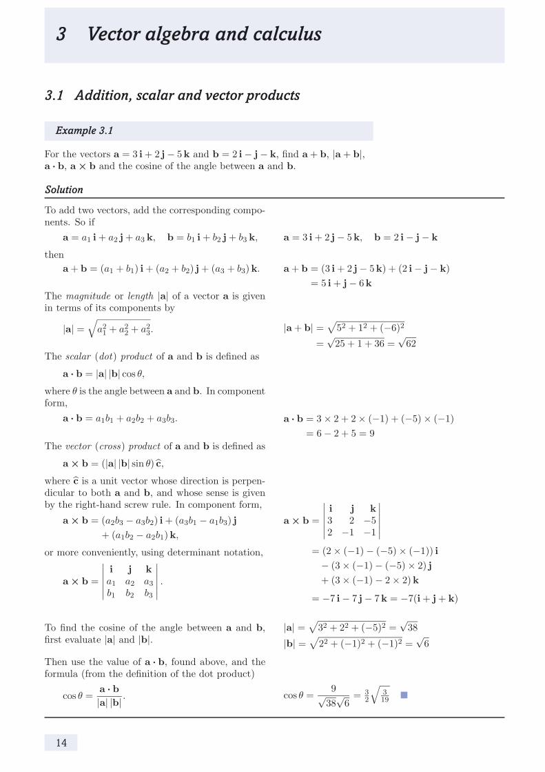
Example 3.1

For the vectors a = 3 i + 2 j− 5 k and b = 2 i − j− k, find a + b, |a + b|, a . b, a × b and the cosine of the angle between a and b.

Solution

To add two vectors, add the corresponding compo-nents. So if

a = a1 i + a2 j + a3 k, b = b1 i + b2 j + b3 k, a = 3 i + 2 j− 5 k, b = 2 i − j − k

then a + b = (a1 + b1) i + (a2 + b2) j + (a3 + b3) k. a + b = (3 i + 2 j− 5 k) + (2 i − j− k)

= 5 i + j− 6 k The magnitude or length |a| of a vector a is given in terms of its components by

2 2|a| = a2 + a2 + a3. |a + b| = 52 + 12 + (−6)2 1 √ √

= 25 + 1 + 36 = 62 The scalar (dot ) product of a and b is defined as

a . b = |a| |b| cos θ,

where θ is the angle between a and b. In component form,

a . b = a1b1 + a2b2 + a3b3. a . b = 3 × 2 + 2 × (−1) + (−5) × (−1) = 6 − 2 + 5 = 9

The vector (cross ) product of a and b is defined as

a × b = (|a| |b| sin θ) c,

where c is a unit vector whose direction is perpen-dicular to both a and b, and whose sense is givenby the right-hand screw rule. In component form,

a × b = (a2b3 − a3b2) i + (a3b1 − a1b3) j + (a1b2 − a2b1) k,

a × b =i j k3 2 −52 −1 −1

or more conveniently, using determinant notation, = (2 × (−1) − (−5) × (−1)) i

a × b = i j ka1 a2 a3

b1 b2 b3

.

− (3 × (−1) − (−5) × 2) j + (3 × (−1) − 2 × 2) k

= −7 i − 7 j − 7 k = −7(i + j + k)

√To find the cosine of the angle between a and b, |a| = first evaluate and b

32 + 22 + (−5)2

22 + (−1)2 + (−1)2 = 6

38= √|a| | |. |b| =

Then use the value of a . b, found above, and the formula (from the definition of the dot product)

a . b 9= 3 3

2 19cos θ = √ √cos θ = . a| |b| | 38 6

14

Comment

In handwritten work, all symbols for vectors should be underlined.

Exercise 3.1

For the vectors a = 3 i − 2 j + k and b = i − 3 j + 5 k, find a + b, |a + b|, a . b, a × b and the cosine of the angle, θ, between a and b.

Steps

(a) Find a + b by adding components.

(b) Now sum the squares of the components of a + b and take the square root, to find |a + b|.

(c) Use the fact that a . b = a1b1 + a2b2 + a3b3 to find a . b.

(d) Use the result

a × b = i j ka1 a2 a3

b1 b2 b3

to find a × b.

(e) Use the definition a . b = |a| |b| cos θ, and the result of part (c), to find cos θ.

Exercise 3.2

In each of the following cases, find a + b, |a + b|, a . b, a × b and the cosine of the angle, θ, between a and b.

(a) a = 2 i − 3 j + k, b = −i + 2 j + 4 k.

(b) a = 2 i + 2 j + k, b = 4 i + 4 j − 7 k.

Exercise 3.3

(a) If a . b = 0, what can be said about the vectors a and b?

(b) If a × b = 0, what can be said about the vectors a and b?

(c) Consider the two vectors a = i + 2 j + k and b = −i + k. Are these two vectors either parallel or perpendicular to each other?

(d) Find the value of (c × d) . c for any non-zero vectors c and d.

Exercise 3.4

Consider the three vectors a = a1 i + a2 j + a3 k, b = b1 i + b2 j + b3 k and c = c1 i + c2 j + c3 k.

(a) Evaluate the scalar triple product a . (b × c), and show that this equals the determinant of the components of a, b and c, that is,

a1 a2 a3

b1 b2 b3

c1 c2 c3

.

(b) Hence, using the properties of determinants, verify that

a . (b × c) = b . (c × a) = c . (a × b).

15

3.2 Position, velocity and acceleration

Example 3.2

If r = 2 cos(3t) i + 2 sin(3t) j + (2t − 1) k is the position vector at time t of a moving particle, find

(a) the velocity of the particle;

(b) the speed of the particle;

(c) the acceleration of the particle;

(d) a unit vector in the direction of the tangent to the trajectory of the particle at r.

Solution

Although the course does not specifically solve problems in particle mechanics, many of the basic ideas concerning the relationship between position, velocity and acceleration vectors do occur.

(a) If the position vector of the particle at time t is r(t), then the velocity vector v(t) is the deriva-tive of r with respect to t. Differentiate each com-ponent, since i, j and k are constant vectors.

(b) The speed of the particle is the magnitude of the velocity vector.

(c) The acceleration vector a(t) is the derivative of the velocity vector with respect to t. This can also be written as the second derivative of r with respect to t.

(d) The curve traced out by the particle as it moves (often called the pathline ) is the geometri-cal representation of the vector function r(t). The derivative dr/dt = v at a point on the curve is a tangent vector to the curve at that point. A unit vector in the direction of this tangent vector is

dr/dt =

v et = . |dr/dt| |v|

r = 2 cos(3t) i + 2 sin(3t) j + (2t − 1) k dr

v = = −6 sin(3t) i + 6 cos(3t) j + 2 k dt

|v| = 36 sin2(3t) + 36 cos2(3t) + 4 √ √

= 40 = 2 10 (since sin2(3t) + cos2(3t) = 1)

dv a = = −18 cos(3t) i − 18 sin(3t) j

dt

From part (a),

v = −6 sin(3t) i + 6 cos(3t) j + 2 k, √

and from part (b), |v| = 2 10.

Hence

1 et = √ (−3 sin(3t) i + 3 cos(3t) j + k).

10

Comment

In this course, we often use the geometrical interpretation of dr/ds as a vector in the direction of the tangent to the curve traced out by the position vector, r(s) = x(s) i + y(s) j + z(s) k, as the parameter s varies. In Example 3.2, the parameter s equals t, and represents time.

16

Exercise 3.5

The position of a moving particle at time t is described by the position b + sin(mt) b and vector r(t) = cos(mt) c, where c are constant,

perpendicular unit vectors, and m is a positive constant. Find the velocity and acceleration vectors of the particle when t = 0. Find also a unit vector in the direction of motion of the particle (that is, in the direction of the velocity vector).

Show that, at any point on the pathline, the velocity vector is perpendicular to the position vector.

Steps

(a) To find the velocity vector v, evaluate the derivative of r(t) with respect to t. Then put t = 0 into your result.

(b) To find the acceleration vector a, evaluate the derivative of v(t) with respect to t. Then put t = 0 into your result.

(c) Evaluate the unit vector et = v/|v|. (d) Show that v . r = 0.

Exercise 3.6

The position vector of a moving particle is

r = 2t i + 1 t3 j− 2 k.6

Find the velocity and acceleration vectors, and show that 44v 2 = 16 + a ,

where v and a are the magnitudes of the velocity and acceleration, respectively.

Exercise 3.7

In plane polar coordinates (r, θ), the unit vectors in the radial and In this course, polar transverse directions are given by coordinates are denoted by

(r, θ), rather than (as er = cos θ i + sin θ j and eθ = − sin θ i + cos θ j, in MST209) by 〈r, θ〉.

respectively, where i and j are Cartesian unit vectors.

(a) If the position vector of a moving particle at time t is r = r er , find Derivatives with respect to expressions for the velocity and acceleration vectors in terms of er time can be made more

and eθ. concise using the Newtonian (dot) notation, with r

(b) For a particle moving in a circle with constant speed, show that the for dr/dt, r for d2r/dt2, etc. acceleration vector is parallel to the position vector, and that the velocity vector is perpendicular to the position vector.

17

3.3 Gradient of a scalar field

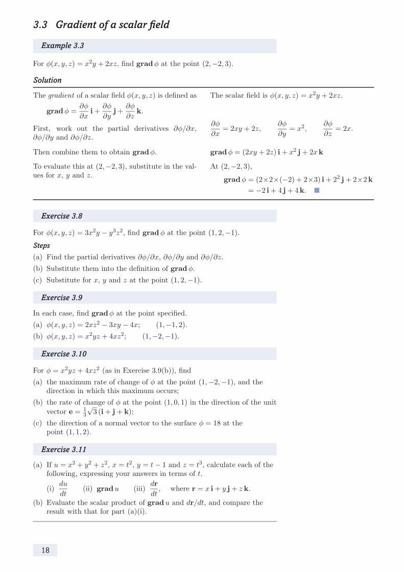
Example 3.3

For φ(x, y, z) = x2y + 2xz, find grad φ at the point (2, −2, 3).

Solution

The gradient of a scalar field φ(x, y, z) is defined as The scalar field is φ(x, y, z) = x2y + 2xz. ∂φ ∂φ ∂φ

grad φ = i + j + k. ∂x ∂y ∂z

∂φ ∂φ ∂φFirst, work out the partial derivatives ∂φ/∂x, = 2xy + 2z, = x2 , = 2x. ∂φ/∂y and ∂φ/∂z. ∂x ∂y ∂z

Then combine them to obtain grad φ. grad φ = (2xy + 2z) i + x2 j + 2x k

To evaluate this at (2, −2, 3), substitute in the val- At (2, −2, 3), ues for x, y and z. grad φ = (2×2×(−2) + 2×3) i + 22 j + 2×2 k

= −2 i + 4 j + 4 k.

Exercise 3.8

For φ(x, y, z) = 3x2y − y3z2, find grad φ at the point (1, 2, −1).

Steps

(a) Find the partial derivatives ∂φ/∂x, ∂φ/∂y and ∂φ/∂z.

(b) Substitute them into the definition of grad φ.

(c) Substitute for x, y and z at the point (1, 2, −1).

Exercise 3.9

In each case, find grad φ at the point specified.

(a) φ(x, y, z) = 2xz2 − 3xy − 4x; (1, −1, 2).

(b) φ(x, y, z) = x2yz + 4xz2; (1, −2, −1).

Exercise 3.10

For φ = x2yz + 4xz2 (as in Exercise 3.9(b)), find

(a) the maximum rate of change of φ at the point (1, −2, −1), and the direction in which this maximum occurs;

(b) the rate of change of φ at the point (1, 0, 1) in the direction of the unit √ vector e = 1 3 (i + j + k);3

(c) the direction of a normal vector to the surface φ = 18 at the point (1, 1, 2).

Exercise 3.11

(a) If u = x2 + y2 + z2 , x = t2 , y = t − 1 and z = t3, calculate each of the following, expressing your answers in terms of t.

du dr(i) (ii) grad u (iii) , where r = x i + y j + z k.

dt dt (b) Evaluate the scalar product of grad u and dr/dt, and compare the

result with that for part (a)(i).

18

3.4 Divergence and curl of a vector field

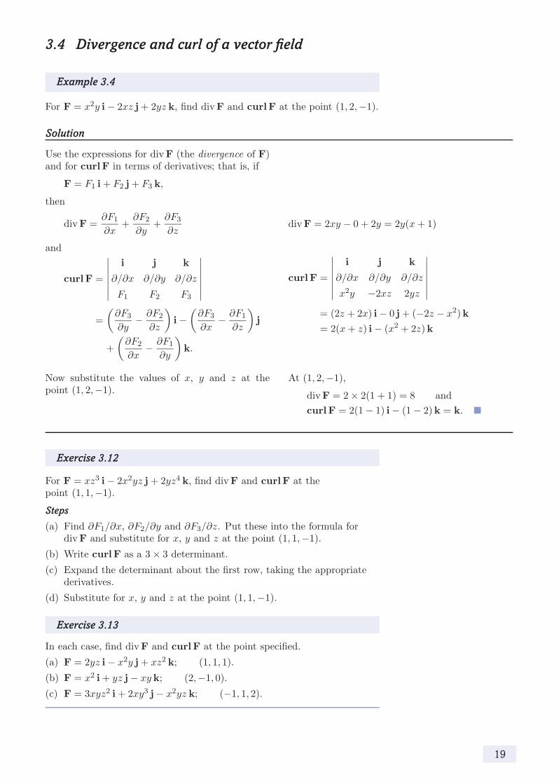
Example 3.4

For F = x2y i − 2xz j + 2yz k, find div F and curl F at the point (1, 2, −1).

Solution

Use the expressions for div F (the divergence of F) and for curl F in terms of derivatives; that is, if

F = F1 i + F2 j + F3 k,

then

∂F1 ∂F2 ∂F3div F = + + div F = 2xy − 0 + 2y = 2y(x + 1) ∂x ∂y ∂z

and

curl F =

i j k

∂/∂x ∂/∂y ∂/∂z

F1 F2 F3

i j k

∂/∂x ∂/∂y ∂/∂zcurl F = 2y −2xz 2yzx

= (2z + 2x) i − 0 j + (−2z − x 2) k∂F3 ∂F2 ∂F3 ∂F1 = − i − − j∂y 2 + 2z) k∂z ∂x ∂z = 2(x + z) i − (x

+ ∂F2 −

∂F1 k. ∂x ∂y

Now substitute the values of x, y and z at the At (1, 2, −1), point (1, 2, −1). div F = 2 × 2(1 + 1) = 8 and

curl F = 2(1 − 1) i − (1 − 2) k = k.

Exercise 3.12

For F = xz3 i − 2x2yz j + 2yz4 k, find div F and curl F at the point (1, 1, −1).

Steps

(a) Find ∂F1/∂x, ∂F2/∂y and ∂F3/∂z. Put these into the formula for div F and substitute for x, y and z at the point (1, 1, −1).

(b) Write curl F as a 3 × 3 determinant.

(c) Expand the determinant about the first row, taking the appropriate derivatives.

(d) Substitute for x, y and z at the point (1, 1, −1).

Exercise 3.13

In each case, find div F and curl F at the point specified.

(a) F = 2yz i − x2y j + xz2 k; (1, 1, 1).

(b) F = x2 i + yz j − xy k; (2, −1, 0).

(c) F = 3xyz2 i + 2xy3 j − x2yz k; (−1, 1, 2).

19

4 Integration of scalar and vector fields

4.1 Line integrals

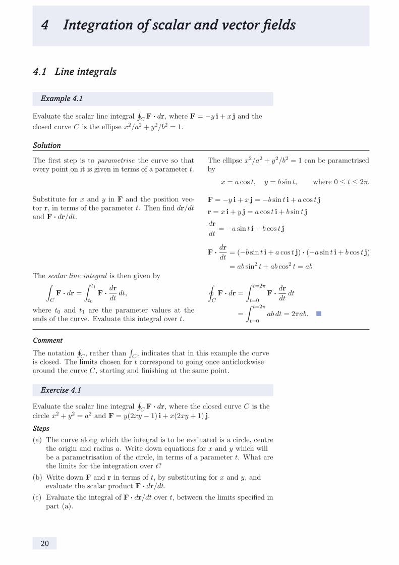
Example 4.1

Evaluate the scalar line integral C F . dr, where F = −y i + x j and the

closed curve C is the ellipse x2/a2 + y2/b2 = 1.

Solution

The first step is to parametrise the curve so that every point on it is given in terms of a parameter t.

Substitute for x and y in F and the position vec-tor r, in terms of the parameter t. Then find dr/dt and F . dr/dt.

The scalar line integral is then given by t1 dr

F . dr = F . dt,dtC t0

where t0 and t1 are the parameter values at the ends of the curve. Evaluate this integral over t.

The ellipse x2/a2 + y2/b2 = 1 can be parametrised by

x = a cos t, y = b sin t, where 0 ≤ t ≤ 2π.

F = −y i + x j = −b sin t i + a cos t j

r = x i + y j = a cos t i + b sin t j

dr = −a sin t i + b cos t j

dt

drF . = (−b sin t i + a cos t j) . (−a sin t i + b cos t j)

dt 2= ab sin2 t + ab cos t = ab

t=2π drF . dr = F . dt

dtC t=0 t=2π

= ab dt = 2πab. t=0

Comment

The notation C , rather than C , indicates that in this example the curve is closed. The limits chosen for t correspond to going once anticlockwise around the curve C, starting and finishing at the same point.

Exercise 4.1

Evaluate the scalar line integral C F . dr, where the closed curve C is the circle x2 + y2 = a2 and F = y(2xy − 1) i + x(2xy + 1) j.

Steps

(a) The curve along which the integral is to be evaluated is a circle, centre the origin and radius a. Write down equations for x and y which will be a parametrisation of the circle, in terms of a parameter t. What are the limits for the integration over t?

(b) Write down F and r in terms of t, by substituting for x and y, and evaluate the scalar product F . dr/dt.

(c) Evaluate the integral of F . dr/dt over t, between the limits specified in part (a).

20

Exercise 4.2

Evaluate the scalar line integral C F . dr for each of the following vector fields F and curves C.

(a) F = (2x + y) i − x j, and C is the quarter-circle, centre the origin and radius 2, between (2, 0) and (0, 2).

(b) F = 3x2 i + (yz + x) j − xy k, and C is the straight line between the points (1, 0, −1) and (2, 1, 3), defined by the parametrisation x = t, y = t − 1, z = 4t − 5 (1 ≤ t ≤ 2).

(c) F = grad φ, where φ = x2yz + yz3, and C is the straight line between the points A (0, 0, 0) and B (1, 1, 1). Check your answer by using the scalar field φ directly.

21

4.2 Surface integrals

Example 4.2

Evaluate the surface integral S xy dA, where S is the region of the plane z = 0 bounded by the curve y = x2 and by the line y = x.

Solution

In Cartesian coordinates,

xy dA = xy dx dy. S S

First draw a diagram showing the region of inte-gration, S. Mark on the diagram the minimum value a and maximum value b of x, for points on the boundary. These values form the limits of the x-integration, provided that this is done after the y-integration.

Find the values of a and b by solving the pair of simultaneous equations

2 y = x , y = x.

Now draw on the diagram a vertical strip showing the limits of the y-integration, which in this case are y = x2 (lower) and y = x (upper).

Write the surface integral as two successive single integrals, one over y (the inner integral) and one over x (the outer integral). Integrate the inner in-tegral (over y, holding x constant). Putting in the limits gives a function of x, g(x) say.

The evaluation of the surface integral is completed by integrating the function g(x) between the limits x = a and x = b.

2 x = x, so x(x − 1) = 0, giving

x = 0 or x = 1 (that is, a = 0 and b = 1).

x=1 y=x

xy dA = xy dy dx S x=0 y=x2

y=x y=x1 4xy dy = x 2y 2y=x2 = x 1 x 2 − 1 x2 2

y=x2

1= 2(x 3 − x 5) (= g(x))

x=1 x=1 1 g(x) dx = 2(x 3 − x 5) dx

x=0 x=0

1 − 1= 1 1 x 4 − 1 x 61 = 1 = 1

2 4 6 0 2 4 6 24 .

22

Comment

The order of integrations in Example 4.2 is not the only possibility. By drawing in a horizontal strip, parallel to the x-axis, the surface integral can be written as √

y=1 x= y

xy dA = xy dx dy, S y=0 x=y

and integration then gives the same result as before.

Exercise 4.3

Evaluate the surface integral S (x2 + y2) dA, where S is the triangle in the

plane z = 0 formed by the lines y = 0, y = x − 1 and x = 2.

Steps

(a) Draw a diagram showing the region of integration, S.

(b) Mark on the diagram the minimum value a and maximum value b of x, for points on the boundary.

(c) Draw on the diagram a strip parallel to the y-axis, and show the lower and upper limits for the y-integration.

(d) Write the surface integral as two successive single integrals.

(e) Evaluate the inner integral (over y, holding x constant).

(f) Complete the evaluation of the surface integral by evaluating the outer integral from x = a to x = b.

Exercise 4.4

Evaluate the surface integral S f (x, y) dA for each of the following functions f and regions of integration S.

(a) f (x, y) = p0 + ρ0g(h0 + x), and S is the rectangle defined by 0 ≤ x ≤ a, 0 ≤ y ≤ b (where p0, ρ0, g and and h0 are constants).

(b) f (x, y) = x − y, and S is the region bounded by the curves y = x2 and 2y = 4x − x .

Exercise 4.5

This question is about the vector field F = y i + x2y j and the circle C with centre the origin and radius 2.

(a) Evaluate the scalar line integral F . dr. C

(b) Evaluate the surface integral S (curl F) . k dA, where S is the interior of the circle C, that is, the region x2 + y2 ≤ 4. Compare your result with the answer to part (a).

4.3 Volume integrals

Example 4.3

Evaluate the volume integral 3x2yz dV , where B is the interior of the B wedge-shaped region with faces in the planes x = 0, y = 0, z = 0, x = 1 and y + z = 1.

23

Solution

In Cartesian coordinates,

f(x, y, z) dV = f(x, y, z) dx dy dz. B B

First draw two diagrams showing

(a) the region of integration, B; (a)

(b) the projection S of B onto the (x, y)-plane. (b)

Now draw, within the region B, a vertical column of rectangular cross-section. The intersections of this column with the top and bottom faces of the region B give the limits of the z-integration, which in this case are z = 0 (lower) and z = 1 − y (upper).

Evaluate the integral of f(x, y, z) over z between z=1−y

3x 2yz dz = 3x y

z z=1−y2 1 2

these limits. 2 z=0 z=0

= 3 x 2 y(1 − y)2 2

The volume integral is now reduced to a surface in- 2 2 2tegral over the projection of the region B onto the B

3x yz dV = 3 x y(1 − y)2 dA S

(x, y)-plane, that is, over the square S (0 ≤ x ≤ 1, x=1 y=1

0 ≤ y ≤ 1). The evaluation of this surface inte- = 3 x 2 (y − 2y 2 + y 3) dy dx2 x=0 y=0gral is completed using the steps of Subsection 4.2.

3y 3 + 1 y=1(Other orders of integration are possible.) = 3

x=1

x 2

2y 2 − 2 4y 4y=0

dx2 1

x=0 x=1 1= 1 x 2 dx = 8 24

x=0

24

Exercise 4.6

Evaluate the volume integral B xz dV , where B is the region inside the semi-circular cylinder x2 + y2 = 1, x ≥ 0, and lying between the planes z = 0 and z = 1.

Steps

(a) Draw two diagrams showing

(i) the region of integration, B;

(ii) the projection S of B onto the (x, y)-plane.

(b) Draw on the region B a vertical column of rectangular cross-section Other orders of integration parallel to the z-axis, and mark on this the upper and lower limits for are possible. the z-integration. Alternatively, this volume

(c) Evaluate the single integral of xz over z between these limits, to integral could be evaluated using cylindrical polar

obtain a function g(x, y), say. coordinates, as shown in (d) Evaluate the surface integral of g(x, y) over the region S of part (a)(ii). Unit 4.

Exercise 4.7

Evaluate the volume integral B f(x, y, z) dV for each of the following functions f and regions of integration B.

(a) f(x, y, z) = x + y + z, and B is the interior of the cube with faces x = 0, x = 1, y = 0, y = 1, z = 0 and z = 1.

(b) f(x, y, z) = z + 3x − 2, and B is the region inside the prism with triangular cross-section y = 0, y = x, x = 2 and lying between the planes z = 0 and z = 1.

5 Dimensions

5.1 Dimensional consistenc y

Example 5.1

In terms of the base dimensions M of mass, L of length and T of time, give the dimensions of each of the following quantities:

area, speed, force. Recall that force is measured

The viscosity, µ, of a fluid is defined by means of an experiment in which the fluid lies between two parallel plates, each of area A and separated by

in newtons (N), where

1N = 1 kg ms−2 .

a small distance h. The upper plate moves with constant speed U when a constant shear force of magnitude F is applied to it, and it is found that

F U A

= µ h

.

Use this result to find the dimensions of viscosity.

25

Solution

The notation [X] is used to mean ‘the dimensions of X’. By definition,

[mass] = M,

[length] = L,

[time] = T.

Dimensional consistency requires that the dimen-sions on either side of a physically meaningful equa-tion should be the same.

Exercise 5.1

Since area is length times length,

[area] = L2 .

Since speed is distance (a length) divided by time,

[speed] = L T−1 .

Since force has the units of mass times length di-vided by time squared,

[force] = M L T−2 .

Rearranging the given equation,

Fh µ = .

AU

From above, [F ] = M L T−2, [A] = L2 and [U ] = L T−1, while [h] = L. Hence

[µ] = [F ][h]

= (M L T−2)(L)

= M L−1 T−1 .[A][U ] (L2)(L T−1)

In terms of M, L and T, give the dimensions of each of the following quantities:

pressure (force per unit area), density (mass per unit volume).

The equation of state for a gas is

p = RρΘ,

where p is the gas pressure, ρ is its density, Θ is its absolute temperature and R is the gas constant. Find the dimensions of R in terms of M, L, T and Θ (the base dimension of temperature).

Steps

(a) Use the dimensions of force, area (both from Example 5.1) and volume to deduce those of pressure and density.

(b) Express R in terms of p, ρ and Θ. Then use the dimensions of these quantities and dimensional consistency to deduce the dimensions of R.

Exercise 5.2

Give the dimensions of each of the following quantities:

acceleration, kinetic energy.

Exercise 5.3

The magnitude F of the gravitational force between two spheres of masses m1 and m2 is given by

Gm1m2F =

2 ,

r

where r is the distance between the two spheres and G is the universal gravitational constant. Find the dimensions of G.

26

5.2 Dimensional analysis

Example 5.2

Assume that the range R (distance from launch to landing) of a projectile,launched from ground level, depends on the mass m, launch speed u andlaunch angle θ of the projectile, and on the magnitude g of the acceleration Recall that angle is adue to gravity, that is, R = f (m, u, θ, g). Use dimensional analysis to find a dimensionless quantity,possible form for the function f . so [θ] = 1.

Solution

First note the dimensions of the given variables.

Assume that the dependent variable is a product of powers of the independent variables, and apply dimensional consistency to write a corresponding equation in terms of dimensions.

Translate into base dimensions, then equate the powers of M, L and T on either side of the equation.

Solve the resulting equations for the powers of the independent variables. Any undetermined power, such as γ here, leads to an undetermined function in the final result. (In fact, the analysis here shows that Rg/u2 is a dimensionless group of variables. Since θ is also dimensionless, it is expected that Rg/u2 = h(θ) for some function h.)

We have [R] = L, [m] = M, [u] = L T−1, [θ] = 1 and [g] = L T−2 .

βθγAssume that R = k mαu gδ, where k is a dimen-sionless constant. Then

α β γ δ[R] = [m] [u] [θ] [g] .

Using the dimensions above, we have

L = Mα(L T−1)β(L T−2)δ

= Mα Lβ+δ T−β−2δ .

Equating powers of M, L and T in turn gives

M: 0 = α, L: 1 = β + δ, T: 0 = −β − 2δ,

with solution

α = 0, β = 2, δ = −1.

Hence R = k u2θγ g−1, where γ is undetermined. We deduce that

2uR = h(θ) ,

g

where h is an undetermined function.

27

Exercise 5.4

Use dimensional analysis to find a possible expression for the magnitude F of the drag force acting on a sphere moving through a fluid, assuming that it depends only on the speed v and radius r of the sphere, and on the density ρ and viscosity µ of the fluid.

Steps

(a) Note the dimensions of the given variables.

(b) Expressing F as a product k vαrβργµδ, use dimensional consistency to relate the dimensions of the variables.

(c) Translate into base dimensions (using step (a)), then equate the powers of M, L and T on either side of the equation.

(d) Solve the resulting equations for α, β, γ, δ, by expressing β, γ, δ in terms of α.

(e) Rearrange the resulting equation for F , from step (b), so that the undetermined power α appears just once. (The resulting quantity which is raised to the power α is a dimensionless group.)

(f) Finally, replace the factor that involves α by an undetermined function of the dimensionless group.

Exercise 5.5

Use dimensional analysis to find a possible expression for the period τ of a pendulum, assuming that it depends only on the mass m of the bob, the length l of the stem, the angular amplitude Φ of the oscillations and the magnitude g of the acceleration due to gravity.

From Example 5.1 and Exercise 5.1,

[F ] = M L T−2 ,

[ρ] = M L−3 ,

[µ] = M L−1T−1 .

28

Solutions to the exercises

Section 1 Integrating the right-hand side by parts, we have

−x −x e −x dx = −x e 1(−e −x) dx Solution 1.1

= −x e −x − e −x + C, so that (a) The differential equation is of first order, and the −x right-hand side can be written as (ex) × (1/y). e y = −(x + 1)e −x + C.

With y in terms of x, the general solution is (b) y

dy = ex

y = Cex − (x + 1).dx

(c) y dy = e x dx, so (d) Putting x = 0 and y = 1, we have

1 = C − 1, giving C = 2, 1 2y 2 = e x + C, leading to so the particular solution for the given condition is y = ± 2(ex + C) (e x + C > 0). y = 2e x − (x + 1).

(d) Putting x = 0 and y = 1, we have Solution 1.4 1 = ± 2(e0 + C),

2 (after the necessary choice of the In each case, the general solution is followed by the giving C = − 1

positive square root). So the particular solution particular solution, and C is an arbitrary constant.

C 1 51satisfying the condition y(0) = 1 is (a) y = 6x3 + x3

; y = 6x3 +6x3

.√y = 2ex − 1 (2e x − 1 > 0, or x > − ln 2).

(b) y = C sec x − 1 cos x; y = sec x − 1 cos x.2 2

λx; λxSolution 1.2 (c) y = (x + C)e y = (x + 2)e .

x2 + 2CIn each case, the general solution is followed by the (d) y = 2(1 + 2x)

; y = x2 − 4

. particular solution. Both A and C are arbitrary 2(1 + 2x) constants. (e) y = Cex − (x 2 + 2x + 2);

p = Ae−ρ0gz/p0 ; p = p0e −ρ0gz/p0(a) . y = 10e x−1 − (x 2 + 2x + 2). 1(b) y = exp 2 ln(x 2 + 1) + C = A x2 + 1; Solution 1.5

y = 5 x2 + 1. (a) A or B (or direct integration)

(c) y = exp(C − cos x) − 1 = Ae− cos x − 1;(b) A or B (c) A or B (d) B (e) A

y = e − cos x − 1. (f ) C (g) B (h) A (i) C (d) p = exp

g ln(Θ0−kz) + C

Rk Solution 1.6 g/(Rk)

= A(Θ0−kz)g/(Rk); Θ0 − kz

p = p0 . (a) The equation is linear, with constant coefficients Θ0 1/3and of second order. The homogeneous equation is

3(e) y = 4 ln 2 + x

+ C ; d2y + 2

dy − 3y = 0.2 − x dx2 dx

2 + x 1/3 (b) The auxiliary equation is λ2 + 2λ − 3 = 0. 3 y = 4 ln + 27 .

2 − x Solving for λ, we have √ −2 ± 4 + 12 Solution 1.3 λ = = −1 ± 2,

2 that is, λ = 1 or λ = −3.

(a) The equation is linear. It is equivalent to The complementary function is

dy − y = x, yc = Aex + Be−3x . dx

so g(x) = −1 and h(x) = x. (c) In this problem, f (x) = e2x, so the trial function is yp = pe2x . Substituting into the differential (b) p(x) = exp g(x) dx = exp (−1) dx = e−x equation, we obtain

2x 2x4pe 2x + 2(2pe 2x) − 3pe = e , so that d −x −x 2x 2x 1(c) (e y) = x e , so 5pe = e or p = 5 .dx

e y =

x e −x dx. The particular integral is yp = 1e2x .−x 5

29

2x(d) The general solution is y = Aex + Be−3x + 1 e . (b) ∂2u

= ∂

(−Aa sin(ax) e −a 2 y )5

(e) The condition y(0) = 1 ∂x2 ∂x

5 gives −a 2 y ;= −Aa2 cos(ax) e1A + B + 1 = or A + B = 0,5 5

and the condition (dy/dx)(0) = 0 gives ∂2u =

∂ (−Aa2 cos(ax) e −a 2 y )

A − 3B + 2 = 0. ∂x ∂y ∂x

−a 2 y ;1Solving for A 5

and B gives A = − 1 and B = 10 . The = Aa3 sin(ax) e

10 particular solution satisfying the given conditions is ∂2u

= ∂

(−Aa2 cos(ax) e −a 2 y )1 −3x + 1 2x y = − 1 e x + 10 e e . ∂y2 ∂y

10 5−a 2 y ;= Aa4 cos(ax) e

Solution 1.7 ∂2u=

∂ (−Aa sin(ax) e −a 2 y )

∂y ∂x ∂yIn each case, the form of the trial function is followed by the general solution and then by the particular solution. Both A and B are arbitrary constants.

−4x;

= Aa3 sin(ax) e −a 2 y = ∂2u

. ∂x ∂y

(a) yp = p e −4x; y = Aex + Bex/5 + 1 e5 Solution 2.2 23 x/5 + 1 −4x y = 10 e x − 5 e e .2 5∂u ∂u

(b) yp = p x ex/5; y = Aex + Bex/5 − 1x ex/5; (a) = cos(x − y); ∂y

= − cos(x − y);4 ∂x

x − ex/5) − 1y = 25 4x ex/5 .16 (e ∂2u ∂2u

= − sin(x − y);(c) yp = p cos x + q sin x; ∂x2 = − sin(x − y),

∂y2

y = A cos( 1 x) + B sin( 1 x) − 1 sin x; ∂2u =

∂2u = sin(x − y). 2 2 3

8y = 3 sin( 1 x) − 1 sin x. ∂x ∂y ∂y ∂x 2 3

∂u ∂u r(d) yp = p1x + p0; y = (A + Bx)e x + 5x + 8; (b) = ln θ; = ; ∂2u

= 0; y = (4x − 8)e x + 5x + 8. ∂r ∂θ θ ∂r2

(e) yp = p cos(3x) + q sin(3x); ∂2u = −

θ

r 2 ;

∂2u ∂2u 1 = = √ √ ∂θ2 ∂r ∂θ ∂θ ∂r θ

. 1 1 y = e −x/2 A cos 2 3x + B sin 2 3x

∂u ∂u2

73 sin(3x); (c) = t cos(st); = s cos(st);− 73 cos(3x) + 19 ∂s ∂t √ √ √

2 1 34 1 y = e −x/2 73 cos 3x + 3 sin 3x ∂2u

= −t2 sin(st); ∂2u

2 219 2 = −s 2 sin(st); − 73 cos(3x) + 192

73 sin(3x). ∂s2 ∂t2

∂2u ∂2u= = cos(st) − st sin(st).

Solution 1.8 ∂s ∂t ∂t ∂s

Trial function is Solution 2.3 3x yp = x (p cos(4x) + q sin(4x)) + re .

(a) ∂u

= 2x e−4t; ∂u

= −4(x2 + y2 + z2) e−4t . General solution is ∂x ∂t

y = A cos(4x) + B sin(4x) + 1x sin(4x) − 25 e . (b) ∂2u

= 0; = −8z e−4t . 8 3x ∂2u

8∂x ∂y ∂z ∂t Particular solution is

8 6 8 3x y = 25 cos(4x) + 25 sin(4x) + 1x sin(4x) − e .8 25 Solution 2.4 1(a) u 0, 4π = sin 0 × 1π = sin 0 = 0 4

Section 2 (b) In Solution 2.2(c), replace s, t by x, y, respectively.

∂u 1

10, 4π = 1π cos 0 × 1π = π;

∂x 4 4 4Solution 2.1 ∂u

1

(a) When y is treated as a constant, e−a 2 y is ∂y 0, 4π = 0 cos 0 × 1π = 0.4

constant, so 1∂u

= −Aa sin(ax) e −a 2 y (c) ∂2u

0, 4π

= −

1π 2 sin

0 × 1π

= 0; 4 4. ∂x2

∂x 1When x is treated as a constant, cos(ax) is constant, ∂2u

0,

0× 1 − 0× 1

0× 1

= 1; π = cos π π sin π4 4 4∂x ∂y 4

so ∂u 1

= −Aa2 cos(ax) e −a 2 y .

∂2u 0, 4π = −02 sin 0 × 1π = 0.4∂y ∂y2

30

(d) The second-order Taylor polynomial is p2(x, y) = 0 + 1π(x − 0) + 0 y − 1π + 1 4 4 2

a . b = −4; a × b = −14 i − 9 j + k; √× 0(x − 0)2 4

cos θ = −√ √ = − 2 21 6. 2 14 21+ 1(x − 0) y − 1π + 1 × 0 y − 1π4 2 4 √ √ (b) a + b = 6 i + 6 j − 6 k; |a + b| = 108 = 6 3;

= 1πx + x y − 1π = xy. 4 4 1a . b = 9; a × b = −18 i + 18 j; cos θ = 3 .

Solution 2.5

The second-order Taylor polynomial is 22 − 1 p2(x, y) = 1 + x + 1 x 2y .2

Solution 2.6 ∂u dx

(a) = 2x; = − sin s;∂x ds ∂u

= 2y; dy

= cos s. ∂y ds

du(b) = 2x(− sin s) + 2y(cos s)

ds du

(c) = −2 cos s sin s + 2 sin s cos s = 0 ds

Solution 2.7 du

(a) = 4

Solution 3.3

(a) If a . b = 0, then either a = 0 or b = 0 or a and b are perpendicular.

(b) If a × b = 0 then a = 0 or b = 0 or a and b are parallel (in the same or opposite directions).

(c) We have a . b = 0 and a × b = 2 i − 2 j + 2 k. = 0 and b Since a = 0, a and b are perpendicular.

(d) (c × d) . c = 0 for any non-zero vectors c and d, because c × d is perpendicular to c and the dot product of perpendicular vectors is zero.

Solution 3.4

(a) b × c = (b2c3 − b3c2) i − (b1c3 − b3c1) j + (b1c2 − b2c1) k

a . (b × c) = a1(b2c3 − b3c2) − a2(b1c3 − b3c1) + a3(b1c2 − b2c1) a1 a2 a3

ds du

= −2 cos s sin2 s + sin3 s + cos3s − 2 cos2s sin s(b) b1 b2 b3ds = .

(This can also be written as c1 c2 c3

(cos s + sin s)(1 − 3 cos s sin s).) (b) Interchanging two rows of a determinant changes du 3 its sign, so

(c) = es (−2s sin(s2) + 3s2 cos(s2))

= − b1 b2 b3

a1 a2 a3

c1 c2 c3

ds a1 a2 a3

b1 b2 b3

c1 c2 c3

b1 b2 b3

c1 c2 c3

a . (b × c) =

Section 3

Solution 3.1 a1 a2 a3

= b . (c × a).=

(a) a + b = (3 i − 2 j + k) + (i − 3 j + 5 k) Similarly, a . (b × c) = c . (a × b).

= 4 i − 5 j + 6 k Solution 3.5 √ (b) |a + b| = 42 + (−5)2 + 62 = 77 (a) r = cos(mt) cb + sin(mt) (c) a . b = 3×1 + (−2)×(−3) + 1×5 = 3 + 6 + 5 = 14 dr

v = = −m sin(mt) c,b + m cos(mt) i j k 3 −2 1 1 −3 5

dt (d) a × b = since d c/dt = 0.b/dt = 0 and d

When t = 0, we have v = −0 c = m b + m c. = (−2 × 5 − 1 × (−3)) i − (3 × 5 − 1 × 1) j dv

b − m 2 sin(mt) + (3 × (−3) − (−2) × 1) k (b) a = dt

= −m 2 cos(mt) c

= −7 i − 14 j − 7 k When t = 0, we have a = −m b − 0 b. 2 c = −m2 √

14 (c) Since |v| = m, we have (e) 32 + (−2)2 + 12 =

12 + (−3)2 + 52 = 35 √ √

|a| = √ v = − sin(mt) b + cos(mt) |b| =

Hence 14 =

et = c. |v|14 35 cos θ, and so

2 (d) Since c = 0, b = 1 and c = 1 (b . b . c . b and 14

cos θ = √ √ = are perpendicular unit vectors), we have 5 . 14 35

v . r = (−m sin(mt) c)b + m cos(mt) b + sin(mt) Solution 3.2 . (cos(mt) c) = 0. √ √

(a) a + b = i − j + 5 k; |a + b| = 27 = 3 3; Hence v and r are perpendicular.

c

31

Solution 3.6 Solution 3.10

(a) r = 2t i + 1 t3 j − 2 k (a) The maximum rate of change of φ is | grad φ| in6the direction of grad φ. At (1, −2, −1), we have (from

dr v = = 2 i + 1 t2 j; a =

dv = t j; Solution 3.9(b))

2dt dt √ 1 v = |v| = 4 + 1 t4 = 16 + t4; a = |a| = |t|.4 2

Hence 4v2 = 16 + t4 = 16 + a4, as required.

grad φ = 8 i − j − 10 k and so | grad φ| = 165.

(b) The rate of change of φ in the direction of e is grad φ . e. At the point (1, 0, 1), we have √

13grad φ = 4 i + j + 8 k and so grad φ . e = 3 3. Solution 3.7

(a) Using the dot notation for time derivatives where appropriate, with position vector r = r er , the velocity is

d v = r = (r er ) = r er + r er .

dt (Note that er is not a constant vector.) Now

er = cos θ i + sin θ j, eθ = − sin θ i + cos θ j, so

er = − sin θ θ i + cos θ θ j = θ eθ.

Hence

v = r er + rθ eθ.

Also

eθ = − cos θ θ i − sin θ θ j = −θ er , and so

(c) The gradient of φ evaluated at the point (1, 1, 2) is normal to the surface φ = 18. The direction of the normal is that of the vector

grad φ = 20 i + 2 j + 17 k.

Solution 3.11 du

(a) (i) = 6t5 + 4t3 + 2t − 2 dt

(ii) grad u = 2t2 i + 2(t − 1) j + 2t3 k

dr(iii) = 2t i + j + 3t2 k

dt dr

(b) grad u . = 4t3 + 2(t − 1) + 6t5 . dt

2 ¨ a = v = r − rθ er + rθ + 2 rθ eθ. This is the same as du/dt in part (a)(i).

(b) We have r = r0 (constant) for a particle moving in a circle (taking the origin to be at the centre of the circle), so that r = 0 and r = 0. The position vector is r = r0 er . From part (a), the velocity vector is

v = r0θ eθ = r0ω eθ, ˙where θ = ω is constant because the speed |v| = |r0θ|

is constant. The acceleration vector is a = −r0ω

2 er , ¨ because θ = ω = 0.

Both of a and r are multiples of er , and so are parallel. Also v . r = 0 (since eθ . er = 0), and so v and r are perpendicular.

Comment This is true in all cases since, applying the Chain Rule for u(x, y, z), where x = x(t), y = y(t), z = z(t), we have

du ∂u dx ∂u dy ∂u dz dr = + + = grad u . .

dt ∂x dt ∂y dt ∂z dt dt

Solution 3.12 ∂2(a) div F =

∂ (xz 3) +

∂ (−2x yz) + (2yz 4)

∂x ∂y ∂z 2 3= z 3 − 2x z + 8yz

At (1, 1, −1), we have

div F = (−1) − 2 × 1 × (−1) + 8 × 1 × (−1) = −7.

(b) curl F =

i j k

∂/∂x ∂/∂y ∂/∂z

xz 2 43 −2x yz 2yz

Solution 3.8 ∂φ ∂φ ∂φ 3(a) = 6xy; = 3x2−3y2z2; = −2y z. ∂x ∂y ∂z

3(b) grad φ = 6xy i + 3(x2 − y2z2) j − 2y z k

(c) At (1, 2, −1), grad φ = 12 i − 9 j + 16 k.

Solution 3.9

(a) grad φ = (2z2 − 3y − 4) i − 3x j + 4xz k

At (1, −1, 2), grad φ = 7 i − 3 j + 8 k.

(b) grad φ = (2xyz + 4z2) i + x2z j + (x2y + 8xz) k

At (1, −2, −1), grad φ = 8 i − j − 10 k.

(c) curl F = (2z4 + 2x2y) i + 3xz2 j − 4xyz k

(d) At (1, 1, −1), we have

curl F = (2 × 1 + 2 × 1 × 1) i + (3 × 1 × 1) j − (4 × 1 × 1 × (−1)) k

= 4 i + 3 j + 4 k.

Solution 3.13

(a) div F = −x2 + 2xz At (1, 1, 1), div F = 1.

curl F = (2y − z2) j − 2(xy + z) k At (1, 1, 1), curl F = j − 4 k.

(b) div F = 2x + z At (2, −1, 0), div F = 4.

32

curl F = −(x + y) i + y j Solution 4.3 At (2, −1, 0), curl F = −i − j.

(a)2(c) div F = 3yz2 + 6xy2 − x y

At (−1, 1, 2), div F = 5.

curl F = −x2z i + 8xyz j + (2y3 − 3xz2) k At (−1, 1, 2), curl F = −2 i − 16 j + 14 k.

Section 4 Solution 4.1 (b) The minimum and maximum values of x are

x = 1 and x = 2 (that is, a = 1 and b = 2). (a) The equations x = a cos t and y = a sin t can be used as a parametrisation for the circle. The values (c) t = 0 and t = 2π will describe beginning and end points of the circle, and will be used as limits for the integration over t in part (c). (Any other choice for which the beginning and end points are the same is also valid.)

(b) F = y(2xy − 1) i + x(2xy + 1) j

= a sin t (2a 2 sin t cos t − 1) i + a cos t (2a 2 sin t cos t + 1) j x=2 y=x−1

(d) (x 2 + y 2) dA = (x 2 + y 2) dy dx r = x i + y j = a cos t i + a sin t j S x=1 y=0

dr = −a sin t i + a cos t j (e)

y=x−1

(x 2 + y 2) dy = x 2 y + 1 3

y=x−1

dt 3y y=0

y=0 dr

3 (x − 1)3F . = −a 2 sin2t (2a 2 sin t cos t − 1) = x 2(x − 1) + 1 dt

2 + a 2 cos t (2a 2 sin t cos t + 1) (f ) x=2

x 3 − x 3 (x − 1)3 dx2 + 1

= a 4 sin(2t)(cos2t − sin2t) + a 2(cos2t + sin2t) x=1 1 3= 1x 4 − 1x 3 + 12 (x − 1)4

x=2 =

2 = 1 2 4 3 x=1 2 = a 4 sin(2t) cos(2t) + a 2a 4 sin(4t) + a t=2π dr

(c) F . dr = F . dt Solution 4.4 C t=0 2π

dt x=a y=b

= ( 1 a 4 sin(4t) + a 2) dt (a) f (x, y) dA = (p0 + ρ0g(h0+x)) dy dx 2

0 S x=0 y=0 2

x=a = − 1a 4 cos(4t) + a t

2π = 2πa2

= b (p0 + ρ0g(h0+x)) dx8 0

x=0Solution 4.2 = ab p0 + ρ0g h0+ 1 a π/2 x=2

y=4x−x 2 2

(a) F . dr = (−8 cos t sin t − 4 sin2t − 4 cos2t) dt (b) f (x, y) dA = (x − y) dy dxC 0

= −2π − 4 S x=0 y=x2 x=2 (The parametrisation used is x = 2 cos t, y = 2 sin t.) = (2x 3 − 4x 2) dx = − 8 2 x=0

3

(b) F . dr = (3t2 − 4t + 5) dt = 6 C 1

(c) F = grad φ Solution 4.5 2π2 2= 2xyz i + (x z + z 3) j + (x y + 3yz 2) k, so (a) F . dr = (−4 sin2t + 16 cos3t sin t) dt 1 C 0

F . dr = 8t3 dt = 2. = −4π C 0

(The parametrisation used is x = t, y = t, z = t.) (The parametrisation used is x = 2 cos t, y = 2 sin t.)

Check: (b) (curl F) . k dA grad φ . dr = grad φ .

dr dt S x=2

y= √

4−x2

AB AB dt =

= dφ

dt = φ(B) − φ(A) x=−2 y=−√ 4−x2

(2xy − 1) dy dx

AB dt x=2 = φ(1, 1, 1) − φ(0, 0, 0) = 2 = −2 4 − x2 dx = −4π

x=−2

33

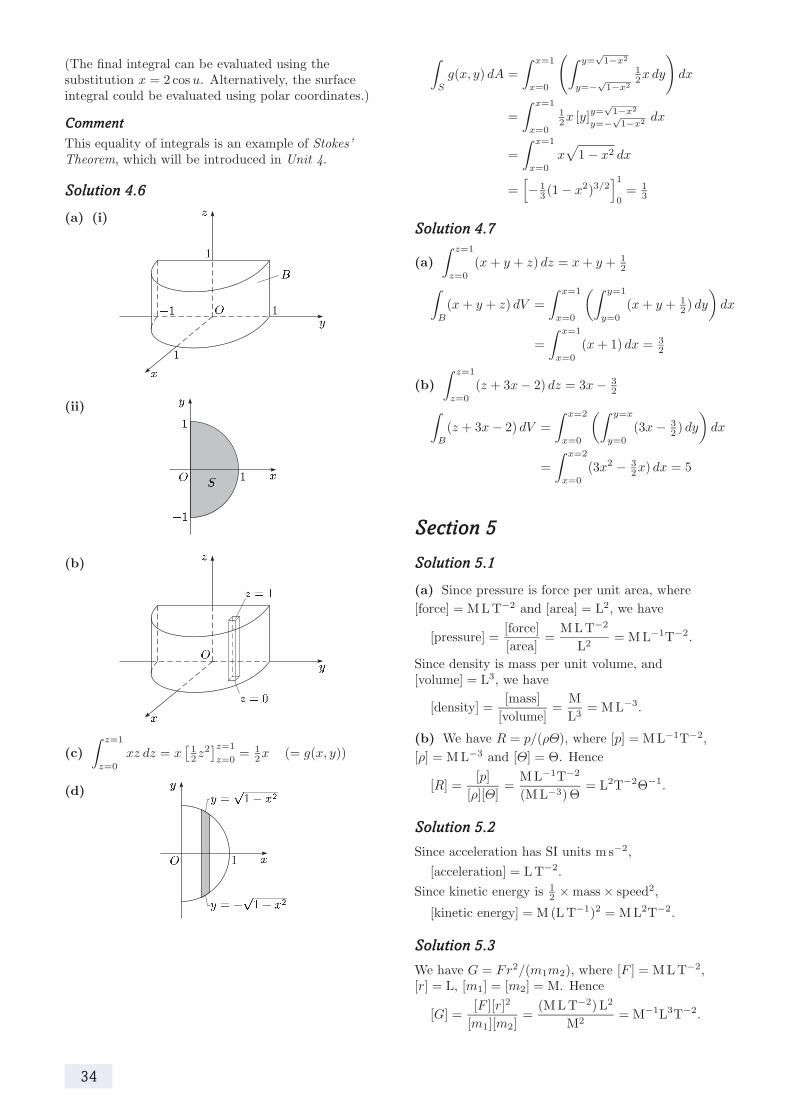
√ x=1 y= 1−x2(The final integral can be evaluated using the

1 substitution x = 2 cos u. Alternatively, the surface g(x, y) dA =

x=0 y=−√ 1−x2

2xdy dx S

integral could be evaluated using polar coordinates.) x=1 √ y= 1−x2

Comment = 1 x [y]y=−√ dx2 1−x2

x=0

This equality of integrals is an example of Stokes’ x=1 Theorem, which will be introduced in Unit 4. = x 1 − x2 dx

x=0 1 2)3/2 = 1

3 (1 − xSolution 4.6 = − 1 30

(a) (i) Solution 4.7 z=1

(a) (x + y + z) dz = x + y + 1 2 z=0 x=1 y=1

(x + y + z) dV = (x + y + 1 2 ) dy dx B x=0 y=0 x=1

3= (x + 1) dx = 2 x=0 z=1

(b) (z + 3x − 2) dz = 3x − 3 2 z=0

(ii) x=2 y=x

(z + 3x − 2) dV = (3x − 3 2 ) dy dx B x=0 y=0 x=2

2 − 3= (3x 2x) dx = 5 x=0

Section 5

(b) Solution 5.1

(a) Since pressure is force per unit area, where

[force] = M L T−2 and [area] = L2, we have

MLT−2

[pressure] = [force]

= = M L−1T−2 .[area] L2

Since density is mass per unit volume, and [volume] = L3, we have

[density] = [mass]

= M

= M L−3 .[volume] L3

(b) We have R = p/(ρΘ), where [p] = M L−1T−2 , (c)

z=1

xz dz = x

1z 2z=1

= 1x (= g(x, y)) [ρ] = M L−3 and [Θ] = Θ. Hence 2 z=0 2z=0

[R] = [p]

=ML−1T−2

= L2T−2Θ−1 .(d) [ρ][Θ] (M L−3)Θ

Solution 5.2

Since acceleration has SI units m s−2 , [acceleration] = L T−2 .

Since kinetic energy is 1 × mass × speed2 ,2

[kinetic energy] = M (L T−1)2 = M L2T−2 .

Solution 5.3

We have G = Fr2/(m1m2), where [F ] = M L T−2 , [r] = L, [m1] = [m2] = M. Hence

2

[G] = [F ][r]

= (M L T−2) L2

= M−1L3T−2 .[m1][m2] M2

34

Solution 5.4

(a) We have [F ] = M L T−2, [v] = L T−1, [r] = L,

[ρ] = M L−3, [µ] = M L−1T−1 .

(b) Taking F = k vαrβργµδ, we have α δ[F ] = [v] [r]β[ρ]γ[µ] .

(c) From step (a), this becomes

ML T−2 = (L T−1)αLβ(M L−3)γ(M L−1T−1)δ

= Mγ+δ Lα+β−3γ−δ T−α−δ .

Equating powers of M, L and T in turn gives M: 1 = γ + δ, L: 1 = α + β − 3γ − δ,

T: −2 = −α − δ.

(d) Expressing β, γ, δ in terms of α, we obtain

β = α, γ = −1 + α, δ = 2 − α.

(e) From step (b), we have

αρ−1+α µ 2−α kµ2 vrρ α

F = k vα r = . ρ µ

(f ) We deduce that a possible form for F is 2µ vrρ

F = h ,ρ µ

where h is an undetermined function.

Comment The dimensionless group vrρ/µ is known as the Reynolds number for this situation. You will see more about this in Units 7 and 8.

Solution 5.5

l τ = h(Φ) ,

g

where h is an undetermined function.

35

Index

absolute temperature 26auxiliary equation 7

base dimensions 25

Chain Rule 13complementary function 7curl (of vector field) 19

density 26differential equation 3, 5, 7

constant-coefficient 7general solution 3–5

explicit form 3, 5implicit form 3, 5

homogeneous 7inhomogeneous 7linear 5, 7non-linear 3of first order 3, 5of second order 7particular solution 3, 4

dimensional analysis 27dimensional consistency 26dimensionless 27dimensionless group 27dimensions 26divergence (of vector field) 19drag force 28

gas constant 26gradient (of scalar field) 18

integrating factor 5integrating factor method 5

kinetic energy 26

Newtonian (dot) notation 17

parametrise 20

partial derivatives 10particular integral 8pathline 16pendulum 28polar coordinates 17pressure 26

range 27Reynolds number 35

scalar field 18scalar line integral 20separation of variables 3shear force 25speed 16Stokes’ Theorem 34surface integral 22

Taylor polynomial (second-order) 11trial function 8

universal gravitational constant 26

variables separated 3vector 14

acceleration 16addition 14cosine of angle between two 14length 14magnitude 14position 16scalar (dot) product 14scalar triple product 15tangent 16unit 16vector (cross) product 14

determinant notation 14velocity 16

vector field 19viscosity 25volume integral 23

36