MSE3 Ch04 Moisture - University of British Columbia88 CHAPTER 4 MoISTURE pure liquid water is given the symbol es.For un-saturated air, e < es. Air can be slightly supersaturated

87

chapter 4

Moisture

4 Water vapor is one of the gases in air. Unlike nitrogen and oxygen, water-vapor concen-tration can vary widely in time and space.

Most people are familiar with relative humidity as a measure of water-vapor concentration because it affects our body’s moisture regulation. But other humidity variables are much more useful in other contexts. Storms get much of their energy from water va-por, because when water vapor condenses or freezes it releases latent heat. For this reason we carefully track water vapor as it rises in buoyant thermals or is carried by horizontal winds. The amount of mois-ture available to a storm also regulates the amount of rain or snow precipitating out. What allows air to hold water as vapor in one case, but forces the vapor to condense in another? This depends on a concept called “saturation”.

saturation Vapor pressure

Vapor pressure All the gases in air contribute to the total pres-sure. The pressure associated with any one gas in a mixture is called the partial pressure. The partial pressure of water vapor in air is called vapor pres-sure. Symbol e is used for water-vapor pressure. Units are pressure units, such as kPa.

saturation Air can hold any proportion of water vapor. However, for humidities greater than a threshold called the saturation humidity, water vapor tends to condense into liquid faster than it re-evaporates. This condensation process lowers the humidity to-ward the equilibrium (saturation) value. The pro-cess is so fast that humidities rarely exceed the equi-librium value. Thus, while air can hold any portion of water vapor, the threshold is rarely exceeded by more than 1% in the real atmosphere. Air that contains this threshold amount of wa-ter vapor is saturated. Air that holds less than that amount is unsaturated. The equilibrium (satura-tion) value of vapor pressure over a flat surface of

Copyright © 2011, 2015 by Roland Stull. Meteorology for Scientists and Engineers, 3rd Ed.

contents

Saturation Vapor Pressure 87Vapor Pressure 87Saturation 87

Humidity Variables 91Mixing Ratio 91Specific Humidity 91Absolute Humidity 91Relative Humidity 92Dew-Point Temperature 92Saturation Level or Lifting Condensation Level (LCL) 93Wet-Bulb Temperature 94More Relationships Between Moisture Variables 96

Total Water 97Liquid and Solid Water 97Total-Water Mixing Ratio 97Precipitable Water 98

Lagrangian Budgets 99Water Conservation 99

Lagrangian Water Budget 99Thermo Diagrams – Part 2: Isohumes 100

Heat Conservation for Saturated Air 101Saturated Adiabatic Lapse Rate 101Thermo Diagrams – Part 3: Saturated

Adiabats 102Liquid-Water, Equivalent, and Wet-Bulb Potential

Temperatures 104

Eulerian Water Budget 107Horizontal Advection 107Precipitation 107Surface Moisture Flux 108Turbulent Transport 109

Humidity Instruments 111

Summary 112Threads 112

Exercises 113Numerical Problems 113Understanding & Critical Evaluation 115Web-Enhanced Questions 117Synthesis Questions 118

“Meteorology for Scientists and Engineers, 3rd Edi-tion” by Roland Stull is licensed under a Creative Commons Attribution-NonCommercial-ShareAlike

4.0 International License. To view a copy of the license, visit http://creativecommons.org/licenses/by-nc-sa/4.0/ . This work is available at http://www.eos.ubc.ca/books/Practical_Meteorology/ .

88 CHAPTER 4 MoISTURE

pure liquid water is given the symbol es. For un-saturated air, e < es. Air can be slightly supersaturated ( e > es ) when there are no surfaces upon which water vapor can condense (i.e., unusually clean air, with no cloud condensation nuclei, and no liquid or ice particles). Temporary supersaturation might occur when the threshold value drops so quickly that condensation does not remove water vapor fast enough. However, photographs of air flow over aircraft wings for both subsonic and supersonic flight through humid air indicate that condensation to form cloud droplets occurs almost instantly. Even at saturation, there is a continual exchange of water molecules between the liquid water and the air. The evaporation rate depends mostly on the temperature of the liquid water. The condensation rate depends mostly on the humidity in the air. At equilibrium these two rates balance. If the liquid water temperature increases, then evaporation will temporarily exceed condensation, and the number of water molecules in the air will in-crease until a new equilibrium is reached. Thus, the equilibrium (saturation) humidity increases with temperature. The net result is that warmer air can hold more water vapor at equilibrium than cooler air. The Clausius-Clapeyron equation describes the relationship between temperature and satura-tion vapor pressure, which is approximately:

e eL

T Ts ov o

≈ℜ

−

·exp ·

1 1 •(4.1a)

where eo = 0.611 kPa and To = 273.15 K are con-stant parameters, and ℜv = 461 J·K–1·kg–1 is the gas constant for water vapor. Absolute temperature in Kelvin must be used for T in eq. (4.1). Because clouds can consist of liquid droplets and ice crystals suspended in air, you must consider saturations with respect to water and ice. Over a flat water surface, use the latent heat of vaporiza-tion L = Lv = 2.5x106 J·kg–1 in eq. (4.1), which gives Lv/ℜv = 5423 K. Over a flat ice surface, use the latent heat of deposition L = Ld = 2.83x106 J·kg–1 , which gives Ld/ℜv = 6139 K. Saturation vapor pressure is listed in Table 4-1 and plotted in Figs. 4.1 and 4.2. These were produced by solving eq. (4.1) on a computer spreadsheet. The exponential-like increase of water-vapor holding ca-pacity with temperature has tremendous impact on clouds and storms. Supercooled (unfrozen) liquid water can exist between temperatures of 0 to –40°C, hence, the curve for saturation over water includes temperatures below 0°C.

Solved Example Find the saturation vapor pressure for T = 21°C?

Solution Given: T = 21°C = 294 KFind: es = ? kPa. Use eq. (4.1) for liquid water.

es = −

( . )·exp ( )·0 611 5423

1273

1303

kPa KK K

= (0.611 kPa)·exp(1.419) = 2.525 kPa

Check: Units OK. Physics OK. Agrees with Table 4-1.Discussion: Compared to average sea-level pressure P = 101.3 kPa, this is roughly 2.5% of the total.

Figure 4.1Saturation vapor pressure over a flat surface of pure water. A blowup of the portion of this curve colder than 0°C is given in the next figure.

Figure 4.2Saturation vapor pressure over flat surfaces of pure liquid water and ice, at temperatures below 0°C. The insert shows difference between saturation vapor pressures over water and ice.

R. STULL • METEoRoLogy FoR SCIENTISTS AND ENgINEERS 89

The Clausius-Clapeyron equation also describes the relationship between water-vapor pressure e and dew-point temperature (Td, to be defined later):

e e

LT To

v o d=

ℜ−

·exp ·

1 1 (4.1b)

Table 4-1. (1) Saturation values of humidity vs. actual air temperature (T). -or- (2) Actual humidities vs. dew-point temperature (Td). Values are for over a flat surface of liquid water. Mixing ratio r and specific humidity q values are for sea-level pressure. Vapor-pressure e and absolute hu-midity ρv values are for any pressure. Subscript s de-notes a saturation value.

For P = 101.325 kPa

T es rs qs ρvs

or

Td e r q ρv

(°C) (kPa) (g/kg) (g/kg) (g/m3)

–20–18–16–14–12

–10–8–6–4–202468

101214161820222426283032343638404244464850

0.1270.1500.1770.2090.245

0.2870.3350.3910.4550.528

0.6110.7060.8140.9371.076

1.2331.4101.6101.8352.088

2.3712.6883.0423.4373.878

4.3674.9115.5146.1826.921

7.7368.6369.627

10.71711.914

13.228

0.780.921.091.281.51

1.772.072.412.803.26

3.774.375.045.806.68

7.668.78

10.0511.4813.09

14.9116.9519.2621.8524.76

28.0231.6935.8140.4345.61

51.4357.9765.3273.5982.91

93.42

0.780.921.091.281.51

1.762.062.402.803.25

3.764.355.015.776.63

7.608.709.95

11.3512.92

14.6916.6718.8921.3824.16

27.2630.7234.5738.8643.62

48.9154.7961.3168.5476.56

85.44

1.091.281.501.752.04

2.372.753.183.674.22

4.855.576.377.288.30

9.4510.7312.1713.7715.56

17.5519.7622.2224.9427.94

31.2734.9338.9643.4048.27

53.6259.4765.8872.8780.51

88.84

BeYonD aLGeBra • clausius-clapeyron

Historical Underpinning To build better steam engines during the indus-trial revolution, engineers were working to discover the thermodynamics of water vapor. Steam engi-neers B.-P.-E. Clapeyron in 1834 and R. Clausius in 1879 applied the principles of S. Carnot (early 1800s), to study isothermal compression of pure water vapor in a cylinder. They measured the saturation vapor pressure at the point where condensation occurred.

Variation of Vapor Pressure with Temperature By repeating the experiment for various tempera-tures, they empirically found that:

dedT

LT

s v

v L= −

−

1 11

ρ ρ

where ρv is the density of water vapor, and ρL is the density of liquid water. But ρL >> ρv (see Appendix B and Table 4-1), thus 1/ ρL << 1/ρv , allowing us to neglect the ρL term:

dedT

LT

s vv≅ ρ

The ideal gas law can be used to relate the wa-ter vapor pressure to the vapor density: es = ρv·ℜv·T, where ℜv is the gas constant for water vapor. Solv-ing for ρv and plugging the result into the eq. above gives:

dedT

L e

Ts v s

v≅ℜ

·

· 2

Use the Separation of Variables method: move all es terms to the left, all T terms to the right:

dee

L dT

Ts

s

v

v≅ℜ 2

Then integrate, taking care with the limits:

dee

L dT

Ts

se

ev

v T

T

o

s

o

∫ ∫≅ℜ 2

where eo is a known vapor pressure at reference tem-perature To. The integration result is:

ln

ee

LT T

s

o

v

v o

≅ −

ℜ−

1 1

Taking the antilog (exp) of both sides gives eq. (4.1).

e eL

T Ts ov o

=ℜ

−

· exp ·1 1

(4.1)

See C. Bohren and B. Albrecht [1998: Atmospheric Thermodynamics, Oxford, 402pp] for details, and for an interesting historical discussion.


Tetens’ formula is an empirical expression for saturation vapor pressure es with respect to liquid water:

e eb T T

T Ts o= −−

· exp

·( )1

2 (4.2)

It includes the variation of latent heat with tempera-ture, where eo = 0.611 kPa, b = 17.2694, T1 = 273.15 K, and T2 = 35.86 K. Although this formula depends on temperature differences (for which °C or K can nor-mally be used), absolute temperature T in units of Kelvins must be used here because the parameters T1 and T2 are given in Kelvins.

Solved Example Compare Tetens’ formula with the Clausius-Clap-eyron equation for a variety of temperatures

Solution Use eqs. (4.1) and (4.2) in a spreadsheet. The result below on a semi-log graph shows the Clausius-Clapeyron equation as a solid line, and Tetens’ formula as a dashed line.

Check: Units OK. Physics OK. Agrees with Table 4-1.Discussion: Both formulae are extremely close over a wide range of temperatures.

Focus • Boiling

Definition: Boiling is the state where ambient atmospheric pressure equals the equilibrium (saturation) vapor pressure: P = es

Derivation of Boiling T vs. z: Because ambient pressure decreases roughly ex-ponentially with height, we can use (1.9b) to replace the left hand side (LHS) of the equation above by P = Po·exp(–z/Hp), where Po = 101.325 kPa is sea level pres-sure (at z = 0), and Hp ≈ 7.29 km is the scale height for pressure. The right hand side (RHS) can be replaced with the Clausius-Clapeyron eq. (4.1), which describes how this boiling pressure is related to T. The net re-sult is:

Pz

He

LT To

po

v

v o· exp ·exp ·−

=

ℜ−

1 1

where Lv /ℜv = 5423 K. Dividing both sides by Po, and using the trick that eo/Po = exp[ln(eo/Po)], gives:

exp exp ln−

=

+ℜ

zH

eP

LTp

o

o

v

v o

1−ℜ

LT

v

v

1

But the first two terms in square brackets on the RHS are constants, and can be grouped as a dimen-sionless constant a. Taking the ln of both sides gives:

zH

LT

ap

v

v=ℜ

−1

Rearranging to solve for temperature T (which equals Tboiling because we had set P = es):

TL

a z Hboilingv v

p=

ℜ+

//

By definition of the Celsius temperature scale, T = 100°C = 373.15 K for boiling at sea level z = 0. Using these values of z and T in the eq. above allows us solve for a, yielding a = 14.53 (dimensionless).

Discussion: At z = 1 km, the eq. above gives Tboiling = 96.6°C, and at z = 2 km, Tboiling = 93.2°C. This is an average decrease of 3.4°C / km. To soften vegetables to the desired tenderness or to prepare meats to the desired doneness, foods must be cooked at a certain temperature over a certain time duration. Slightly cooler cooking temperatures must be compensated with slightly longer cooking times. Thus, boiled foods take longer to cook at higher alti-tude because the boiling temperature is cooler.

science Graffito

“I think, therefore I am.” — René Descartes.


huMiDitY VariaBLes

Mixing ratio The ratio of mass m of water vapor to mass of dry air is called the mixing ratio, r:

rm

mwater vapor

dry air=

(4.3)

where mdry air = mtotal air – mwater vapor . To put this into a more useful form, divide the numerator and denominator by a common volume to get a ratio of densities, substitute the ideal gas law for each gas, and assume a common temperature for all gases. The result is:

re

P e=

−ε · •(4.4)

where ε = ℜd/ℜv = 0.622 gvapor/gdry air = 622 g/kg is the ratio of gas constants for dry air to that for water vapor. Eq. (4.4) says that r is proportional to the ratio of partial pressure of water vapor (e) to par-tial pressure of the remaining gases in the air (P – e), where P is total air pressure. The saturated mixing ratio, rs, is similar to eq. (4.4), except with saturation vapor pressure es in place of e.

re

P ess

s=

−ε ·

•(4.5)

Examples of mixing ratio values are given in Table 4-1, for air at sea level, where the Clausius-Clapeyron equation or Tetens’ formula is used to find es . Although units of mixing ratio are “g/g” (i.e., grams of water vapor per gram of dry air), it is usu-ally presented as “g/kg” (i.e., grams of water vapor per kilogram of dry air) by multiplying the “g/g” value by 1000. By convention in meteorology we don’t reduce the ratio “g/g” to 1, because the numer-ator and denominator represent masses of different substances that must be discerned in mass budgets.

specific humidity The ratio of mass m of water vapor to mass of total (moist) air is called the specific humidity, q, and to a good approximation is given by:

qm

m

qm

m

water vapor

total air

water vapor

dry

=

=

aair water vaporm+

(4.6)

or q

eP e

eP e

qe

P

d=

+=

− −

≈

εε

εε

ε

··

··( )

·

1 (4.7)

where ε = 0.622 g/g = 622 g/kg, and P is pressure. Specific humidity q has units of g/g or g/kg. For saturation specific humidity, qs :

qe

P e

qe

P ee

P

ss

d s

ss

s

s

=+

=− −

≈

εε

εε

ε

··

··( )

·1

(4.8)

Both the saturation mixing ratio and saturation specific humidity depend on ambient pressure, but the saturation vapor pressure does not. Thus, in Table 4-1 the vapor pressure numbers are abso-lute numbers that can be used anywhere, while the other humidity variables are given at sea-level pres-sure and density. The saturation values of mixing ratio and specific humidity can be calculated for any other ambient pressure using eqs. (4.5) and (4.8).

absolute humidity The concentration ρv of water vapor in air is called the absolute humidity, and has units of grams of water vapor per cubic meter of air (g/m3). Abso-lute humidity is essentially a partial density:

ρvwater vaporm

Volume= (4.9)

where m is mass and Vol is volume. Absolute hu-midity can be reformulated using the ideal gas law for water vapor:

ρvv

eT

=ℜ ·

(4.10)

where ℜv = 4.61x10–4 kPa·K–1·m3·g–1 is the gas con-stant for water vapor. Alternately, by replacing tem-perature T using the ideal gas law for dry air:

ρε ρ

ε ρvd

deP e

eP

=−

≈· ·

· · (4.11)

where ρd is the density of dry air, e is the vapor pressure, ε = ℜd/ℜv = 622 g/kg, and P is total air pressure. As discussed in Chapter 1, dry-air density is roughly ρd = 1.225 kg/m3 at sea level, and varies with altitude, pressure, and temperature according to the ideal gas law. The saturated value of absolute humidity, ρvs, is found by using es in place of e in the equations above:

ρvss

v

eT

=ℜ ·

(4.12)

or

ρε ρ

ε ρvss d

s

sd

eP e

eP

=−

≈· ·

· · (4.13)


relative humidity The ratio of the actual amount of water vapor in the air compared to the equilibrium (saturation) amount at that temperature is called the relative hu-midity, RH:

RH qq

rrs

v

vs s

%%100

= = ≈ρρ

•(4.14)

where e is vapor pressure, q is specific humidity, ρv is absolute humidity, r is mixing ratio, and subscript s indicates saturation. Relative humidity regulates the amount of net evaporation that is possible into the air, regardless of the temperature. At RH = 100% no net evaporation occurs because the air is already saturated. Varia-tion of mixing ratio with RH is shown in Fig. 4.3.

Dew-point temperature The temperature to which air must be cooled in order to become saturated at constant pressure is called the dew-point temperature, Td , (also known as the dew point). It is given by eq. (4.1) or found from Table 4-1 by using vapor pressure e in place of es and Td in place of T. Making those substi-tutions and solving for Td yields:

TT L

eed

o

v

o= −

ℜ

−1

1

· ln (4.15a)

with eo =0.611 kPa, To =273 K, ℜv/Lv =1.844x10–4 K–1. Eq. (4.15a) can be combined with the definition of mixing ratio r to give:

TT L

r Pe rd

o

v

o= −

ℜ+

−

11

ln·

·( )ε •(4.15b)

where ε = ℜd/ℜv = 0.622 gvapor/gdry air . Saturation (equilibrium) with respect to a flat surface of liquid water occurs at a slightly colder temperature than saturation with respect to a flat ice surface. With respect to liquid water, use L = Lv in the equation above, where Td is called the dew-point temperature. With respect to ice, L = Ld , and Td is called the frost-point temperature (see the “Saturation” subsection for values of L). If Td = T, the air is saturated. The dew-point depression or temperature-dew-point spread (T – Td) is a relative measure of the dryness of the air. Td is usually less than T (except during supersaturation, where it might be a fraction of a de-gree warmer). If air is cooled below the initial dew-point temperature, then the dew-point temperature drops to remain equal to the air temperature, and

Solved Example Find the saturation values of mixing ratio, specific humidity, and absolute humidity for air of tempera-ture 0°C and pressure 50 kPa.

Solution Given: T = 0°C, P = 50 kPaFind: rs = ? g/kg, qs = ? g/kg, ρvs = ? g/m3

es = 0.611 kPa was found directly from Table 4-1 be-cause it does not depend on P.

Use eq. (4.5) for rs:rs = [0.622·(0.611 kPa)] / [50 kPa - 0.611 kPa] = 0.00770 g/g = 7.70 g/kg

Use eq. (4.8) for qs:qs = 0.622·(0.611 kPa)/50 kPa = 0.00760 g/g = 7.60 g/kg

Use eq. (4.12) for ρvs:ρvs = (0.611 kPa)/[(461 J·K–1·kg–1)·(273 K)] = 0.00485 kg·m–3 = 4.85 g·m–3 .

Check: Units OK. Physics OK.Discussion: The first two values are roughly double those for sea-level pressure (see Table 4-1). The reason is that although the partial pressure of water vapor held in the air is the same, partial pressure of dry air is less. The last value equals the value in Table 4-1, because there is no P dependence.

Figure 4.3Mixing ratio at sea level vs. relative humidity and temperature.


the excess water condenses or deposits as dew, frost, fog, or clouds (see the Cloud and Precip. chapters). Dew-point temperature is easy to measure and provides the most accurate humidity value, from which other humidity variables can be calculated (see Humidity Instruments section at the end of this chapter). When dew (sweat) forms on the outside of a cold beverage can or bottle, you know that the outside of the beverage container is colder than the dew-point temperature of the surrounding air.

saturation Level or Lifting condensation

Level (LcL) When unsaturated air is lifted, it cools at the dry adiabatic lapse rate. If lifted high enough, the tem-perature will drop to the dew-point temperature, and clouds will form. Dry air (air of low relative humidity) must be lifted higher than moist air. Sat-urated air needs no lifting at all. Hence, LCL is a measure of humidity. When lifting non-cloudy air, the height at which saturation just occurs (with no supersaturation) is the saturation level or the lifting condensation level (LCL). For convective (cumuliform) clouds, cloud base occurs there. LCL height (distance above the height where T and Td are measured) for cumuliform clouds is very well approximated by:

z a T TLCL d= −·( ) •(4.16a)

where a = 0.125 km/°C. The pressure PLCL at the LCL is

P P bT T

TLCLd

Cp

= −−

ℜ· ·

/

1 (4.16b)

where b = a·Γd = 1.225 (dimensionless), CP/ℜ = 3.5 (dimensionless), and P is the pressure at the initial

Solved Example Find the LCL height and pressure, if T = 20°C and Td = 10°C at P = 95 kPa.

Solution Given: T = 20°C, Td = 10°C, P = 95 kPa.Find: zLCL = ? km , PLCL = ? kPa

Use eq. (4.16a) zLCL = (0.125km/°C)·(20 – 10°C) = 1.25 km above the starting height

Use eq. (4.16b) PLCL = (95 kPa)·[1 – 1.225·(20–10°C)/293K]3.5 = 81.8 kPa

Check: Units OK. Physics OK. Discussion: Reasonable height for cumulus cloud base. Also, since pressure decreases about 10 kPa for each increase of 1 km of altitude near the surface, the pressure answer is also reasonable.

Solved Example Find the relative humidity for air of T = 20°C and e = 1 kPa.

Solution Given: T = 20°C , e = 1 kPaFind: RH = ? %

From Table 4-1 at T = 20°C : es = 2.371 kPa.Use eq. (4.14): RH = 100% · (1 kPa / 2.371 kPa) = 42%.

Check: Units OK. Physics OK.Discussion: The result does not depend on P.

Solved Example Given desert conditions with a temperature of 30°C and pressure of 100 kPa, find the dew-point tempera-ture for a relative humidity of 20%.

Solution Given: T = 30°C , P = 100 kPa, RH = 20%Find: Td = ? °C

From Table 4-1, es = 4.367 kPa. Use eq. (4.14): e = 0.2·(4.367 kPa)= 0.8734 kPaWe could use eq. (4.15) to solve for Td, but it is easier to look up the answers in Table 4-1. Td = 5°C.

Check: Units OK. Physics OK.Discussion: The result does not depend on P. This dry air would need to be cooled 25°C before condensa-tion would occur.

Solved Example Find the dew point for r = 10 g/kg and P = 80 kPa.

SolutionGiven: r = 0.01 gvapor/gair, P = 80 kPaFind: Td = ? °C

Use eq. (4.15b): Td = [(1/(273K) – (1.844x10–4 K–1)· ln{ [(80kPa)·(0.01gvapor/gair)] / [(0.611kPa)·( (0.01gvapor/gair) + (0.622gvapor/gair)] }]–1 = [(1/(273K) – (1.844x10–4 K–1)·ln(2.07)]–1 = 283.4K . Thus, Td = 283.4 – 273 = or 10.4°C

Check: Units OK. Magnitude OK. Discussion: This humidity might occur in the trop-ics, with a surface temperature warmer than 30°C.


height where temperature T and dew-point Td are measured, such as at the surface. Don’t forget to use Kelvin for the T in the denominator. These expressions do not work for stratiform (advective) clouds, because these clouds are not formed by air rising vertically from the underlying surface. Air in these clouds blows at a gentle slant angle from a surface hundreds to thousands of kilo-meters away. Regardless of whether cumuliform clouds exist, the LCL or saturation level can be used as a measure of humidity. It also serves as a measure of total wa-ter content for saturated (cloudy) air. For cloudy air, the saturation level is the altitude to which one must lower an air parcel for all of the liquid or solid water to just evaporate. Eqs. (4.16) do not apply to this situ-ation.

Wet-Bulb temperature When the bulb of a glass thermometer is covered by a cloth sleeve that is wet, this wet bulb becomes cooler than the actual (dry bulb) air temperature T because of the latent heat associated with evapora-tion of water. Drier ambient air allows more evapo-ration, causing the wet-bulb temperature Tw to cool significantly below the air temperature. For saturat-ed air there is no net evaporation and the wet-bulb temperature equals that of the dry bulb. You can find the humidity from the difference between the dry and wet-bulb temperatures. This difference, called the wet-bulb depression (T – Tw), is a mea-sure of the relative dryness of the air. To work properly, the sleeve or wick must be wet with clean or distilled water. The wet bulb should be well ventilated by blowing air past it (aspirat-ed psychrometer) or by moving the thermometer through the air by twirling it around on the end of a short chain (sling psychrometer). Usually psy-chrometers have both wet and dry-bulb thermom-eters mounted next to each other. Let Tw represent the wet-bulb temperature, and rw represent the wet-bulb mixing ratio in the air adjacent to the wet-bulb after water has evaporated into it from the sleeve. Because the latent heat used for evaporation comes from the sensible heat associ-ated with cooling, a simple heat balance gives:

C T T L r rp w v w·( ) ·( )− = − − (4.17)

where T and r are ambient (dry-bulb) air tempera-ture and mixing ratio, respectively, Cp is the specific heat of air at constant pressure, and Lv is the latent heat of vaporization.

Solved Example At a pressure of 100 kPa, what is the mixing ratio if the dry and wet-bulb temperatures of a psychrometer are 20°C and 14°C, respectively? Use the equations here, not the look-up tables or graphs.

Solution Given: T = 20°C , Tw = 14°C , P = 100 kPaFind: r = ? g/kg

First, solve eq. (4.18): rw =

622

1 631 9017 67 18

11

g/kg

kPa kPa°C

( . )·( )·exp. ·− −

88 243 51

° °CC +

−.

rw = 10.13 g/kg.

Then solve eq. (4.19):r = (10.13g/kg) – [0.40224 (g/kg)/°C]·(20–14°C) = 7.72 g/kg.

Check: Units OK. Physics OK.Discussion: Now we can compare our answer with the data in graph (Fig. 4.4). Using Tw = 14°C along the ordinate, and T – Tw = 20 – 14 = 6°C as the dew-point depression along the abscissa, we find that our answer agrees with the graph. Obviously, for every-day use, it is easier to use the psychrometric graph, or the cor-responding psychrometric tables that are published in other books.

Solved Example For the previous solved example, use its inputs and result to calculate the relative humidity. Again, don’t use the look-up tables or graphs yet.

Solution Given: T = 20°C , r= 7.72 g/kg, P = 100 kPaFind: RH = ? %

First, use Tetens’ formula (4.2) , with the trick that ΔT = T(K) – T1(K) = [T(°C)+273] – 273 = T(°C) , and remem-bering that for temperature differences: 1°C = 1 K .

es = + −0 611

17 2694 2020 273 16

. ·exp. ·( )

( . )(kPa)

KK 335 86. K

es = 2.34 kPa.

Next, use this in eq. (4.5):

rs = −[ ] =( )· .

. .622 2 34101 325 2 34

g/kg kPakPa

14.7g//kg

Finally, use eq. (4.14): RH = 100%·(r/rs) RH = 100% · (7.72/14.7) = 52.5%

Check: Units OK. Physics OK.Discussion: What a lot of work. If we instead had used psychrometric graph (Fig. 4.5) with Tw = 14°C T – Tw = 6°C , we would have found almost the same relative humidity much more easily.


If the wet and dry-bulb temperatures and ambi-ent pressure P are measured or otherwise known, the desired mixing ratio r can be found by first find-ing rw:

rb P

c T CT C

ww

w

=−

+

−

ε

α· ·exp

· ))(°

(°1

(4.18)

Then:

r r T Tw w= − −β ·( ) (4.19)

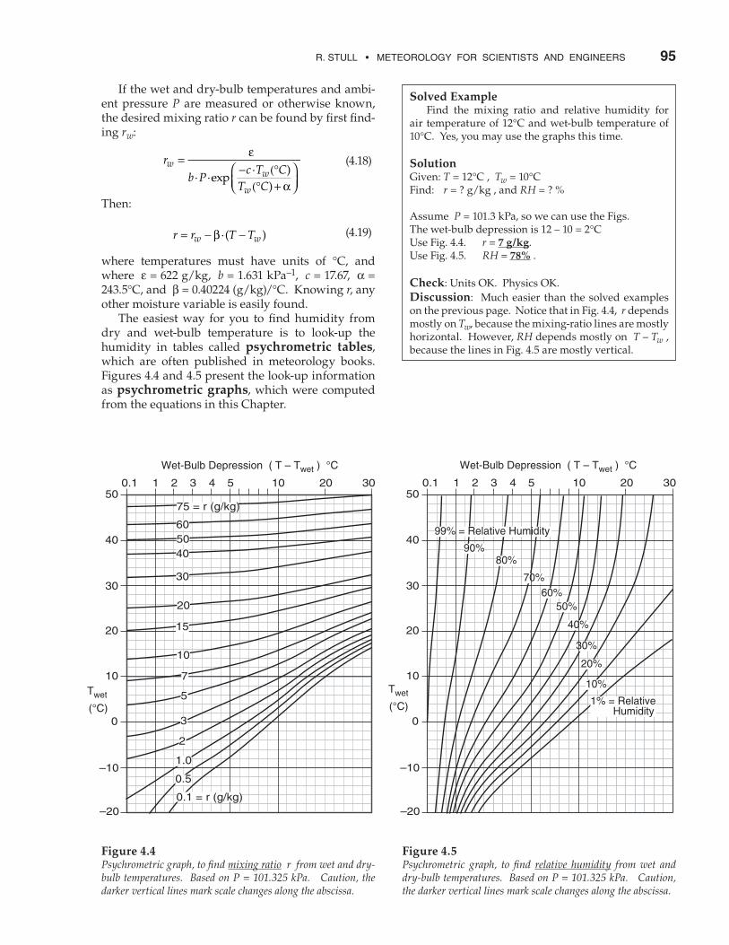
where temperatures must have units of °C, and where ε = 622 g/kg, b = 1.631 kPa–1, c = 17.67, α = 243.5°C, and β = 0.40224 (g/kg)/°C. Knowing r, any other moisture variable is easily found. The easiest way for you to find humidity from dry and wet-bulb temperature is to look-up the humidity in tables called psychrometric tables, which are often published in meteorology books. Figures 4.4 and 4.5 present the look-up information as psychrometric graphs, which were computed from the equations in this Chapter.

Figure 4.4Psychrometric graph, to find mixing ratio r from wet and dry-bulb temperatures. Based on P = 101.325 kPa. Caution, the darker vertical lines mark scale changes along the abscissa.

Figure 4.5Psychrometric graph, to find relative humidity from wet and dry-bulb temperatures. Based on P = 101.325 kPa. Caution, the darker vertical lines mark scale changes along the abscissa.

Solved Example Find the mixing ratio and relative humidity for air temperature of 12°C and wet-bulb temperature of 10°C. Yes, you may use the graphs this time.

Solution Given: T = 12°C , Tw = 10°C Find: r = ? g/kg , and RH = ? %

Assume P = 101.3 kPa, so we can use the Figs.The wet-bulb depression is 12 – 10 = 2°CUse Fig. 4.4. r = 7 g/kg.Use Fig. 4.5. RH = 78% .

Check: Units OK. Physics OK.Discussion: Much easier than the solved examples on the previous page. Notice that in Fig. 4.4, r depends mostly on Tw, because the mixing-ratio lines are mostly horizontal. However, RH depends mostly on T – Tw , because the lines in Fig. 4.5 are mostly vertical.


To create your own psychrometric tables or graphs, first generate a table of mixing ratios in a spreadsheet program, using eqs. (4.18) and (4.19). I assumed a standard sea-level pressure of P = 101.325 kPa for the figures here. Then contour the resulting numbers to give Fig. 4.4. Starting with the table of mixing ratios, use eqs. (4.2), (4.5), and (4.14) to create a new table of relative humidities, and contour it to give Fig. 4.5. All of these psychrometric tables and graphs are based on Tetens’ formula (eq. 4.2). Finding Tw from Td is a bit trickier, but is possible using Normand’s Rule:

• Step 1: Find zLCL using eq. (4.16).

• Step 2: T T zLCL d LCL= − Γ · (4.20)

• Step 3: T T zw LCL s LCL= + Γ · (4.21)

where Γs is the moist lapse rate described later in this chapter, Γd = 9.8 K/km is the dry rate, and TLCL is the temperature at the LCL. Normand’s Rule tells us that Td ≤ Tw ≤ T. Normand’s rule is easy to implement on a thermo diagram. Although isohumes and moist adiabats on thermo diagrams are not introduced until later in this chapter, I demonstrate Norman’s rule here for future reference. Follow a dry adiabat up from the given dry-bulb temperature T, and follow an isohume up from the given dew point Td (Fig. 4.6). At the LCL (where these two isopleths cross), follow a moist adiabat back down to the starting pressure to give the wet-bulb temperature Tw.

More relationships Between Moisture

Variables Units of g/g must be used for r and q in the rela-tionships below: q

rr

=+1

(4.22)

q v

d v=

+ρ

ρ ρ (4.23)

q

eP

LT T

o

v o d=

ℜ

−

ε··exp ·

1 1 (4.24)

e

rr

P=+ε

· (4.25)

r v

d=ρρ

(4.26)

Solved Example Find the wet-bulb temperature for air at sea level with temperature 30°C and dew point 24°C.Assume Γs = 3.78 °C/km for this case.

Solution Given: T = 30°C , Td = 24°C , P = 101.3 kPaFind: Tw = ?°C

Use Normand’s Rule:Step 1, solve eq. (4.16): zLCL = (0.125 km/°C)·(30 – 24°C) = 0.75 km.Step 2, solve eq. (4.20): TLCL = 30 – (9.8 K/km)·(0.75 km) = 22.65 °C.Step 3, solve eq. (4.21): Tw = 22.65 + (3.78 °C/km)·(0.75 km) = 25.5°C.

Check: Units OK. Physics OK.Discussion: The resulting wet-bulb depression is (T – Tw) = 4.5°C.

Figure 4.6Demonstration of Normand’s rule on a thermo diagram. It shows how to find wet-bulb temperature Tw, given T and Td.

Focus • Why so Many Moisture Variables?

Vapor pressure, mixing ratio, specific humidity, absolute humidity, relative humidity, dew point de-pression, saturation level, and wet bulb temperature are different ways to quantify moisture in the air. Why are there so many? Some variables are useful because they can be measured. Others are useful in conservation equa-tions for water substance, for describing physical characteristics of the air, or for describing how life is affected by humidity. Often we are given or can mea-sure one moisture variable, but must convert it to a different variable to use it. (continues on next page)


For air that is not excessively humid:

r q≈ •(4.27a)

r qs s≈ •(4.27b)

totaL Water

Liquid and solid Water In clouds, fog, or air containing falling precipita-tion, one measure of the amount of liquid water in the air is the liquid water content (LWC). It is defined as

ρLWCliq waterm

Vol= . (4.28)

where mliq.water is mass of liquid water suspended or falling through the air, and Vol is the air volume. Typical values in cumulus clouds are 0 ≤ ρLWC ≤ 5 g/m3. It can also be expressed in units of kgliq.water/m3. LWC is the liquid-water analogy to the absolute humidity for water vapor. Another measure is the liquid-water mixing ratio:

rm

mLliq water

dry air= .

(4.29)

where mliq.water is the mass of liquid water that is imbedded as droplets within an air parcel that con-tains mdry air mass of dry air. A similar ice mixing ratio can be defined:

rm

miice

dry air=

(4.30)

Both mixing ratios have units of kgwater/kgair, or gwater/kgair. Liquid water content is related to liquid-water mixing ratio by

rLLWC

air=ρρ

(4.31)

where ρair is air density.

total-Water Mixing ratio Define total-water mixing ratio rT as the mass of water of all phases (vapor, liquid, and ice) per mass of dry air:

r r r rT L i= + + •(4.32a)

Focus • Why so Many Moisture Variables? (continuation)

Directly and easily measurable variables include wet-bulb temperature and dew-point temperature. Wet-bulb temperature is easy to measure by putting a wet cloth sleeve around the bulb of a thermometer, and ventilating the wet bulb. However, it is difficult to convert this into other humidity variables, which is why psychrometric tables and graphs have been de-veloped. Dew point is measured by chilling a mirror until dew forms on it. It is one of the most accurate measurements of humidity. Absolute humidity can be measured by shining electromagnetic radiation (infrared, ultraviolet, or microwave) across a path of humid air. The attenua-tion of the signal is a measure of the number of water vapor molecules along the path. Relative humidity can be measured by: 1) expan-sion or contraction of organic fibers such as human hairs; 2) the change in electrical conductivity of a car-bon powder emulsion on a glass slide; and 3) by how it affects the capacitance across a plastic dielectric. Relative humidity is extremely important because it affects the rate of evaporation from plants, animals, and the soil. Mixing ratio or specific humidity are not usually measured directly, but are extremely useful because they are conserved within air parcels moving verti-cally or horizontally without mixing. Namely, heat-ing, cooling, or changing the pressure of an air parcel will not change the mixing ratio or specific humidity in unsaturated air. Lifting condensation level, or saturation level, can be used to estimate the altitude of cloud base for con-vective (cumulus) clouds. Vapor pressure is neither easily measured nor di-rectly useful. However, it is important theoretically because it describes from first principles how satura-tion humidity varies with temperature.

Solved Example Find the liquid water mixing ratio in air at sea lev-el, given a liquid water content of 3 g/m3.

SolutionGiven: ρLWC = 3 gwater/m3. Sea level.Find: rL = ? gwater/kgdry air.Assume standard atmosphere, and use Table 1-5 from Chapter 1 to get: ρair = 1.225 kgair/m3 at sea level.

Use eq. (4.31): rL = (3 gwater/m3)/(1.225 kgair/m3) = 2.45 gwater/kgdry air. = 2.45 g/kg

Check: Units OK. Physics OK. Magnitude reasonable.Discussion: Liquid, solid and water vapor might ex-ist together in a cloud.


where r is the water-vapor mixing ratio, rL is the liquid-water mixing ratio, and ri is the ice mixing ratio. All these mixing ratios have units of kgwater/kgair, or gwater/kgair. Similar total-water variables are defined in terms of specific humidity and absolute humidity. Liquid-water cloud droplets can exist unfrozen in air of temperature less than 0°C. Thus, it is pos-sible for ice and liquid water to co-exist in the same air parcel at the same time, along with water vapor. For negligible precipitation, eq. (4.32a) is approx-imately:

r rT = for unsaturated air •(4.32b)

r r r rT Ls i= + + for saturated air •(4.32c)

where the water-vapor mixing ratio is assumed to equal its saturation value rs when liquid or ice is present. The words saturated air means cloudy air, and unsaturated air means non-cloudy air. Total water is nearly conserved, in the sense that the amount of water lost or created via chemical re-actions is small compared to the amounts advected with the wind or associated with precipitation. Thus, the change of total water in a volume can be calculated by the amount of water of all phases that enters or leaves the volume. Recall that saturation water-vapor mixing ratio decreases as temperature decreases (see Table 4-1). Thus, given some initial amount of total water rT, eq. (4.32c) says that liquid or solid water must increase as temperature and rs decrease, in order that the sum of all water phases remain constant in saturated air. Clouds or fog form when the total water content of the air exceeds the saturation (equilibrium) value. Because total water is an important factor in cloud and precipitation formation, budget equations for total water are presented in the next main section.

precipitable Water If all the vapor, liquid, and solid water within a column of air in the atmosphere were to precipitate out, the resulting depth of water on the Earth’s sur-face (or in a rain gauge) is called the precipitable wa-ter, dW. It is given by

dr

gP PW

T

liqB T= −

··( )

ρ •(4.33)

where rT is average total-water mixing ratio, PB and PT are ambient air pressures at the bottom and top of the column segment, |g|= 9.8 m·s–2 is gravitation-al acceleration magnitude, and ρliq = 1000 kg·m–3 is density of liquid water.

Solved Example If an average of 5 g/kg of total water existed in the troposphere, between 100 kPa and 30 kPa, what is the precipitable water depth?

SolutionGiven: rT = 0.005 kg/kg, PB = 100 kPa, PT = 30 kPa Find: dW = ? m

Use eq. (4.33): and recall from Appendix A that 1 kPa = 1000 kgair·m·s–2 . Thus, dw = { (0.005 kg/kg) / [(9.8 m·s–2)·(1000 kg·m–3) ] } · ( 100 – 30 kPa) · (1000 kgair·m·s–2 /kPa) = 0.036 m = 3.6 cm (≈ 1.4 inches).

Check: Units OK. Physics OK.Discussion: Why so much precipitation? Because we used an unrealistically large mixing ratio over the whole depth of the troposphere. Although 5 g/kg is reasonable near the surface, higher in the troposphere the air is much colder and can hold much less water vapor.

Solved Example Saturated air at sea level with T = 10°C contains 3 g/kg liquid water. Find the total water mixing ratio.

SolutionGiven: T = 10°C, rL = 3 g/kgFind: rT = ? g/kg.Assume: No ice.

Use Table 4-1 because it applies for sea level. Other-wise, solve equations or use thermo diagram.At T = 10°C: rs = 7.66 g/kg from the table.

Use eq. (4.32c): rT = rs + rL + ri = 7.66 + 3 + 0 = 10.66 g/kg

Check: Units OK. Physics OK.Discussion: According to Table 4-1, the air would need to warm to 15°C to evaporate all liquid water


If the mixing ratio varies with height, then the full column can be broken into smaller column seg-ments of near-uniform mixing ratio. The result-ing precipitable-water depths per segment can be summed to give the total precipitable-water depth. Precipitable water is sometimes used as a humid-ity variable. The bottom of the atmosphere is warm-er than the mid and upper troposphere, and can hold the most water vapor. In a pre-storm cloudless environment, contributions to the total-column pre-cipitable water thus come mostly from the bound-ary layer. Hence, precipitable water can serve as one measure of boundary-layer total water that could serve as the fuel for thunderstorms later in the day. See the Thunderstorm chapters for a sample map of precipitable water. In the real atmosphere, winds can advect mois-ture into a column to replace that lost from pre-cipitation. Consequently, the total rainfall amount observed at the surface after storm passage is often much greater than the precipitable water at any in-stant. Some microwave and infrared sensors on satellites (see the Remote Sensing chapter) measure precipitable water averaged over large depths of the troposphere.

LaGranGian BuDGets

Moist air parcels have two additional proper-ties that were unimportant for dry air. One is the amount of water in the parcel, which is important for determining cloud formation and precipitation amounts. The second is the latent heat released or absorbed when water changes phase, which is criti-cal for determining the buoyancy of air parcels and the energy of thunderstorms.

Water conservation

Lagrangian Water Budget If you follow an air parcel as it moves, and as-sume no turbulent mixing with the environment, then the Lagrangian water budget is

∆∆

=rt

ST * * (4.34)

where S** is a Lagrangian net source of water. This source could be evaporation from adjacent liquid water, or it could be a loss of water falling from the parcel as precipitation (causing negative S**). If there is no source or loss, then there is no change of total water content. Phase changes must

science Graffito

“The best way to have a good idea is to have lots of ideas.” — Linus Pauling.

science Graffito

“Great ideas often receive violent opposition from mediocre minds.” — Albert Einstein.


compensate each other to maintain constant total water. Thus, for no net source:

( ) ( )r r r r r ri initial i finalL L+ + = + + •(4.35a)

For the special case of no ice, this reduces to:

( ) ( )r r r rL Linitial final+ = + •(4.35b)

On a thermodynamic diagram, conservation of total water corresponds to following an isohume of constant mixing ratio as a parcel rises or descends. Thus, it is total water mixing ratio that is conserved, not dew-point temperature.

Thermo Diagrams – Part 2: Isohumes Two classes of information are included on thermo diagrams: states and processes. State of the air is defined by temperature, pressure, and moisture. Two processes are unsaturated (dry) and saturated (moist) adiabatic vertical movement, such as experienced by air parcels rising through the atmosphere. Processes can change the state. The chart background of vertical isotherms and horizontal isobars was introduced in Chap-ters 1 (Fig. 1.4) and 3 (Fig. 3.3). Here we will overlay isohumes of constant saturation-mixing-ratio state over the background (Fig. 4.7). To use the thermo-diagram background of P vs. T for isohumes, we need to describe rs as a function of P and T [abbreviate as rs(P, T)]. Eq. (4.5) gives rs(P, es) and the Clausius-Clapeyron eq. (4.1) gives es(T). So combining these two equations gives rs(P, T).

Figure 4.7Thermodynamic diagram with isohumes of mixing ratio.

Solved Example An air parcel at sea level has a temperature of 20°C and a mixing ratio of 10 g/kg. If the air is cooled to 10 °C, what is the liquid water content?

SolutionGiven: T = 20°C, r = 10 g/kgFind: rL = ? gliq/gair at T = 10°C

Use Table 4-1 because it applies for sea level. Other-wise, solve equations or use a thermo diagram. As-sume no other sources or sinks.

Initially:rs = 14.91 g/kg from the table, at T = 20°C.Air is initially unsaturated, because r < rs. Unsaturated air has no liquid water: rL = 0.Assume no ice at these warm temperatures. (r + rL)initial = (10 + 0) (g/kg) = 10 g/kg

Finally:After cooling the air to 10°C, Table 4-1 shows that the max amount of vapor that can be held in the air at equilibrium is r = rs = 7.66 g/kg. However, total water must be constant if it is conserved. Use eq. (4.35b): 10 g/kg = (r + rL)final = 7.66 g/kg + rL finalThus, rL final = 10 g/kg – 7.66 g/kg = 2.34 g/kg

Check: Units OK. Physics OK.Discussion: Some liquid water has formed in the air parcel, so it is now a cloud or fog.

Solved Example Use Fig. 4.7 to answer (A) these questions (Q).

SolutionQ: What is the saturation mixing ratio for air of temperature 0°C and pressure 40 kPa?A: Follow the T = 0°C isotherm vertically, and the P = 40 kPa isobar horizontally, to find where they intersect. The saturation mixing ratio (dot-ted diagonal) line that crosses through this inter-section is the one labeled: rs ≈ 10 g/kg.

Q: What is the actual mixing ratio for air of dew point 0°C and pressure 40 kPa? A: This is the same intersection point yielding the same numerical answer, but because dew-point temperature was used, the answer represents the actual mixing ratio. r ≈ 10 g/kg.

Q: What is the dew-point temperature for air of mixing ratio 20 g/kg and pressure 80 kPa? A: From the intersection of the diagonal dotted line for r = 20 g/kg and the horizontal isobar for P = 80 kPa, go vertically straight down to find Td ≈ 21°C.


But to draw any one isohume (i.e., for any one value of rs), we need to rearrange the result to give T(P, rs):

TT L

r Pe ro

v

v

s

o s= −

ℜ+

−

11

·ln·

·( )ε (4.36)

where eo = 0.611 kPa, To = 273 K, ε = 0.622 g/g, and ℜv/L = 0.0001844 K–1. Be sure to use g/g and not g/kg for rs. The answer is in Kelvin. Thus, pick any fixed rs to plot. Then, for a range of P from the bottom to the top of the atmosphere, solve eq. (4.36) for the corresponding T values. Plot these T vs. P values as the isohume line on a thermo diagram. Use a spreadsheet to repeat this calculation for other values of rs, to plot the other isohumes. Eqs. (4.36) with (4.15b) are similar. Thus, you can use isohumes of T(P, rs) to also represent isohumes of Td(P, r). Namely, you can use isohumes to find the saturation state rs of the air at any P and T, and you can also use the isohumes to describe the process of how Td changes when an air parcel of constant r rises or descends to an altitude of different P.

heat conservation for saturated air

Saturated Adiabatic Lapse Rate The unsaturated (dry) adiabatic lapse rate, Γd = 9.8 K/km, was discussed earlier. It is the temper-ature decrease ( –∆T/∆z = Γd ) an air parcel would experience as it moves vertically in the atmosphere into regions of lower pressure. No mixing or heat transfer across the skin of the parcel can occur for an adiabatic process. Although the word “dry” ap-pears, this lapse rate applies to moist as well as dry air, but only if the air is unsaturated (i.e., not cloudy). Air cools adiabatically as it rises, and warms as it descends. Saturated (cloudy) air also cools as it rises and warms as it descends, but at a lesser rate than a dry parcel. The reason is that, by definition, a saturated parcel is in equilibrium with the liquid drops. If the parcel then rises and cools, it is no longer in equilib-rium, and some of the water-vapor molecules con-dense as a new equilibrium is approached. During condensation, latent heat is released into the air, par-tially compensating the adiabatic cooling. The opposite is true during descent. Some of the cloud droplets evaporate and remove heat from the air, partially compensating the adiabatic warming. For saturated air, the decrease of temperature with height ( –∆T/∆z = Γs ) in clouds and fog is given by the saturated-adiabatic lapse rate, Γs:

Solved Example Calculate the dew point of air at pressure 80 kPa and mixing ratio 1 g/kg.

SolutionGiven: P = 80 kPa, r = 1 g/kgFind: Td = ?°C

Use eq. (4.15b):

Td = − ⋅

⋅

1273

0 000184

0 001 80

KK

g/g kPa

-1.

ln( . ) ( ))

. ( . . )0 611 0 001 0 622

1

kPa g/g⋅ +

−

= [0.003663 – 0.0001844·ln{0.210}]–1 = 253.12 K = –20°C

Check: Units OK. Physics OK. Agrees with Fig. 4.7. Discussion: We would have found the same nu-merical answer if we asked for the temperature cor-responding to air at 80 kPa that is saturated with rs = 1 g/kg with rL = 0. For this situation, we would have used eq. (4.36).


Γ sp

s v

d

v s

p d

g

C

r LT

L r

C T

=+ℜ

+ℜ

·

··

· ·

· ·

1

12

2ε

(4.37a)

This is sometimes called the moist adiabatic lapse rate. The value of specific heat Cp is a function of humidity, and can be found using eq. (3.2). If the variation of specific heat with humidity is neglected for simplicity, then (4.37a) simplifies to:

Γ Γs ds

s

a r T

b r T= ⋅

+ ⋅[ ]+ ⋅

1

1 2

( / )

( / ) •(4.37b)

where Γd = 9.8 K/km, a = 8711 K, and b = 1.35x107 K2. As shown in the solved example, eq. (4.37b) dif-fers from (4.37a) by roughly 1%, so it is often accurate enough for most applications. In both equations the saturation mixing ratio rs varies with temperature, and must be used in units of g/g. Also, temperature must be Kelvin. Near the ground in humid conditions, the value of the moist adiabatic lapse rate is near 4 K/km, and often changes to 6 to 7 K/km in the middle of the troposphere. At high altitudes where the air is cold-er and holds less water vapor, the moist rate nearly equals the dry rate of 9.8 K/km. Instead of a change of temperature with height, the moist lapse rate can be written as a change of temperature ∆T with change of pressure ∆P:

∆∆

=ℜ( ) ⋅ + ( ) ⋅

⋅ +⋅ ⋅

TP

C T L C r

PL r

C

d p v p s

v s

p

/ /

12 ε⋅⋅ℜ ⋅

d T2

(4.38a)

where saturation mixing ratio rs varies with T.The corresponding simplified form is:

∆∆

=+[ ]

+

TP

a T c r

P b r Ts

s

· ·

· ( · / )1 2 •(4.38b)

where a = 0.28571, b = 1.35x107 K2 , c = 2488.4 K.

Thermo Diagrams – Part 3: Saturated Adiabats

Recall that two processes shown in thermo dia-grams are unsaturated (dry) and saturated (moist) adiabatic vertical movement, such as experienced by air parcels rising through the atmosphere. Un-

Solved Example Find the moist adiabatic lapse rate near sea level for T = 26°C, using (a) the actual specific heat, and (b) the specific heat for dry air. (c) Also find ∆T/∆P for a rising saturated air parcel.

Solution Given: T = 26°C = 299 K , P = 101.325 kPaFind: Γs = ? °C/km

In general, we would need to calculate the saturation mixing ratio using eqs. (4.5) and (4.1). However, for this scenario, we can use Table 4-1 for simplicity, be-cause sea-level pressure was specified. Thus: rs = 21.85 g/kg = 0.0219 g/g.

(a) Using eq. (3.2), the actual specific heat is: Cp = 1023 J·kg–1·K–1. Thus: |g|/Cp = 9.58 K/km Lv/Cp = 2444 K. Lv/ℜd = 8711 K.Plugging these into eq. (4.37a) gives:

Γs =⋅ +

⋅

( . )( . ) ( )

9 58 10 0219 8711

299K

kmg/g K

K

+⋅ ⋅ ⋅

12444 8711 0 0219 0 622

299

( ) ( ) ( . ) .

( )

K K g/g

K 22

= (9.58 K/km)·[1.638]/[4.307] = 3.70 K/km

(b) Eq. (4.37b) uses Cp for dry air:

Γs =⋅ +

⋅

( . )( . ) ( )

9 8 10 0219 8711

299K

kmg/g K

K

111 35 10 0 0219

299

7 2

2+× ⋅

( . ) ( . )

( )

K g/g

K

= (9.8 K/km)·[1.638] / [4.307] = 3.73 K/km.

(c) Use eq. (4.38b):

∆∆

=+[ ]T

P0 28571 299 2488 4 0 0219. ·( ) ( . ·( . ))K K g/g

PP K· [ . ·( . )/( ) ]1 1 35 10 0 0219 2997 2 2+ ×

g/g K

= (32.49K) / P

Assume P = 101.325 kPa at sea level: ∆T/∆P = 0.32 K/kPa

Check: Units OK. Physics OK.Discussion: Don’t forget for answers (a) and (b) that lapse rates are the rate of cooling with altitude. As ex-pected the rate of cooling of a rising cloudy air parcel is less than the 9.8 K/km of a dry parcel. Also, method (b) is accurate enough for many situations. Normally, pressure decreases as altitude increases, thus answer (c) also gives cooling for negative ∆P.


saturated processes were previously indicated by overlaying isentropes (dry adiabats) on the back-ground (Chapter 3, Fig. 3.3). Here we will add satu-rated adiabats, also known as moist adiabats. Moist adiabats show how cloudy air changes tem-perature as it rises or sinks. Unfortunately, eq. (4.38) does not directly give the temperature of a parcel at any pressure height. Instead, one must solve the equation recursively, stepping upward in altitude (toward decreasing P) from an initial temperature at P = 100 kPa. Each step must take a small-enough pressure-height increment that the moist lapse rate does not change significantly from one step to the next. For each step, compute:

T TTP

P P2 1 2 1= + ∆∆

⋅ −( ) (4.39)

where (∆T/∆P) is from eq. (4.38). For example, use pressure height increments of ∆P = (P2 – P1) = – 0.1 kPa all the way from P = 100 kPa up to P = 10 kPa. Repeat the calculations start-ing from five initial temperatures at P = 100 kPa: T1 = 40, 20, 0, –20, and –40°C. Fig. 4.8 shows the results of such calculations on a spreadsheet. The calculations were done in units of Kelvin, and then converted to Celsius for plotting. The moist adiabats are labeled with their starting temperature at P = 100 kPa, as discussed next. [The solved example at right uses coarser vertical increments of ∆P = – 2 kPa. This is too coarse, and can cause 5°C errors at 20 kPa.]

Focus • spreadsheet thermodynamics

Saturated (Moist) Adiabatic Lapse Rate The iteration process of computing the θw = 20°C moist adiabat is demonstrated here. First, set up a spreadsheet with the following row and column headers:

A B C D E1 Moist Adiabat Example2 ∆P(kPa)= 234 P (kPa) T(°C) es(kPa) rs(g/g) ∆T/∆P5 100 20.0

where the starting pressure and temperature have been entered as numbers, and where the pressure in-crement of ∆P = 2 kPa has also been entered. Because ∆T/∆P in eq. (4.38b) depends on rs, which in turn depends on es, there are the two extra columns C and D in the spreadsheet above. Two typical mistakes are to forget to convert T into Kelvins before using it, or to forget to use g/g for r. In cell C5, you can enter eq. (4.1), which is: =0.611*EXP(5423*((1/273.15)-(1/(B5+273.15))))Then, in cell D5, enter eq. (4.5): =0.622*C5/(A5-C5)Next, in cell E5, enter eq. (4.38b): =(0.28571*(B5+273.15)+(2488.4*D5)) / (A5*(1+(13500000*D5/((B5+273.15)^2))))In cell A6, increment the pressure: =A5-$B$2Finally, in cell B6 enter eq. (4.39): =B5-(E5*$B$2)where the previous 2 eqs referred to B2 as an absolute reference ($B$2 on some spreadsheets). Finally, select cells C5:E5 and fill them down one row. Then, select all of row 6; namely cells A6:E6, and fill down about 45 rows. The result is shown below, where we have not shown rows 8 to 43 to save space:

A B C D E1 Moist Adiabat Example2 ∆P(kPa)= 234 P (kPa) T(°C) es(kPa) rs(g/g) ∆T/∆P5 100 20.00 2.368 0.0151 0.3606 98 19.28 2.262 0.0147 0.3697 96 18.54 2.158 0.0143 0.379··· ··· ··· ··· ··· ···44 22 –52.28 0.006 0.0002 2.76645 20 –57.82 0.003 0.0001 3.007

Discussion: Columns A and B can be plotted as the 20°C moist adiabat. For other moist adiabats, duplicate these cells, but with different starting T in cell B5. The vertical pressure increment ∆P = 2 kPa is much too coarse to give an accurate value near the top of the graph (i.e., at low pressures). When I repeat the calcu-lation with ∆P = 0.1 kPa, I find T = –60.93 at P = 20 kPa. Even smaller increments would be better.

Figure 4.8Thermodynamic diagram with moist adiabats, labeled by wet-bulb potential temperature θw, or by liquid-water potential temperature θL.


Liquid-Water, Equivalent, and Wet-Bulb Potential Temperatures

Recall from the Heat chapter that potential tem-perature θ is conserved during unsaturated adiabatic ascent or descent. However, if an air parcel contain-ing water vapor is lifted above its LCL, then con-densation will add latent heat, causing θ to increase. Similarly, if the air contains liquid water such as cloud drops, when it descends some of the drops can evaporate, thereby cooling the air and reducing θ. However, we can define new variables that are conserved for adiabatic ascent or descent, regardless of any evaporation or condensation that might occur. One is the equivalent potential temperature θe:

θ θθ

θev

p

v

pd

LC T

rL

Cr≈ +

≈ +

··

· · •(4.40)

Another is liquid water potential temperature, θL:

θ θθ

θLv

pL

v

pdL

LC T

rL

Cr≈ −

≈ −

··

· · •(4.41)

where Lv = 2.5x106 J·kg–1 is the latent heat of vapor-ization, Cp is the specific heat at constant pressure for air (Cp is not constant, see the Heat chapter), T is the absolute temperature of the air, and mixing ratios (r and rL) have units of (gwater/gair). The last approximation in both equations is very rough, with Lv/Cpd = 2.5 K·(gwater/kgair)–1. Both variables are conserved regardless of wheth-er the air is saturated or unsaturated. Consider un-saturated air, for which θ is conserved. In eq. (4.40), water-vapor mixing ratio r is also conserved during ascent or descent, so the right side of eq. (4.40) is con-stant, and θe is conserved. Similarly, for unsaturated air, liquid water mixing ratio rL = 0, hence θL is also conserved in eq. (4.41). For saturated air, θ will increase in a rising air parcel due to latent heating, but r will decrease as some of the vapor condenses into liquid. The two terms in the right side of eq. (4.40) have equal but opposite changes that balance, leaving θe conserved. Similarly, the two terms on the right side of eq. (4.41) balance, due to the minus sign in front of the rL term. Thus, θL is conserved. By subtracting eq. (4.41) from (4.40), we can see how θe and θL are related:

θ θθ

e Lv

pT

LC T

r ··

·≈ +

(4.42)

where the total water mixing ratio (g/g) is rT = r + rL. Although θe and θL are both conserved, they are not equal to each other.

Solved Example Compare on a thermo diagram dry and moist adiabats starting at T = 20°C at P = 100 kPa.

SolutionGiven: T = 20°C at P = 100 kPa.Plot: θ = 20°C and θw = 20°C.

Use curves from Fig. 4.8 and Fig. 3.3.

Check: Slopes look reasonable. Labels match.Discussion: Moist-adiabat temperature decreases more slowly than dry, because condensational latent heating partially compensates for adiabatic cooling.

Solved Example Air at pressure 80 kPa and temperature 0°C is satu-rated, & holds 2 g/kg of liquid water. Find θe and θL.

Solution:Given: P = 80 kPa, T = 0°C = 273K , rL = 2 g/kg.Find: θe = ? °C, θL = ? °C

First, do preliminary calculations shared by both eqs:Rearrange eq. (3.12) to give: (θ/T) = (Po/P)0.28571 = (100kPa/80kPa) 0.28571 = 1.066 Thus, θ = 291K = 18°CAt 80 kPa and 0°C, solve eq. (4.5) for rs = 4.7 g/kgThen use eq. (3.2): Cp = Cpd·(1 +1.84·r) = (1004.67 J·kg–1·K–1) ·[1+1.84·(0.0047 g/g)] = 1013.4 J·kg–1·K–1. Thus, Lv/Cp = 2467 K/(gwater/gair) and (Lv/Cp)·(θ/T) = 2630 K/(gwater/gair)

Use eq. (4.40): θe = (18°C) + (2630 K/(gwater/gair))·(0.0047) = 30.4 °C

Use eq. (4.41): θe = (18°C) – (2630 K/(gwater/gair))·(0.002) = 12.7 °C

Check: Units OK. Physics OK. Magnitudes OK.Discussion: The answers are easier to find using a thermo diagram (after you’ve studied the Stability chapter). For θe , find the θ value for the dry adiabat that is tangent at the diagram top to the moist adiabat. For θL, follow a moist adiabat down to where it crosses the (2 + 4.7 = 6.7 g/kg) isohume, and from there follow a dry adiabat to P = 100 kPa.


We can use θe or θL to identify and label moist adiabats. Consider an air parcel starting at P = 100 kPa that is saturated but contains no liquid water (r = rs = rT). For that situation θL is equal to its initial temperature T (which also equals its initial potential temperature θ at that pressure). A rising air parcel from this point will conserve θL, hence we could la-bel the moist adiabat with this value (Fig. 4.9). An alternative label starts from same saturated air parcel at P = 100 kPa, but conceptually lifts it to the top of the atmosphere (P = 0). All of the water vapor will have condensed out at that end point, heating the air to a new potential temperature. The potential temperature of the dry adiabat that is tan-gent to the top of the moist adiabat gives θe (Fig. 4.9). [CAUTION: On some thermo diagrams, equivalent po-tential temperature is given in units of Kelvin.] In other words, θL is the potential temperature at the bottom of the moist adiabat (more precisely, at P = 100 kPa), while θe is the potential temperature at the top. Either labeling method is fine — you will probably encounter both methods in thermo dia-grams that you get from around the world. Wet-bulb potential temperature (θw) can also be used to label moist adiabats. For θw, use Nor-mand’s rule on a thermo diagram (Fig. 4.10). Know-ing temperature T and dew-point Td at initial pres-sure P, and plot these points on a thermo diagram. Next, from the T point, follow a dry adiabat up, and from the Td point, follow an isohume up. Where they cross is the lifting condensation level LCL. From that LCL point, follow a saturated adiabat back down to the starting altitude, which gives the wet-bulb temperature Tw. If you continue to fol-low the saturated adiabat down to a reference pres-sure (P = 100 kPa), the resulting temperature is the wet-bulb potential temperature θw (see Fig. 4.10). Namely, θw equals the θL label of the moist adiabat that passes through the LCL point. Labeling moist adiabats with values of wet-bulb potential tempera-ture θw is analogous to the labeling scheme for the dry adiabats, which is why I use θw here. To find θe(K) for a moist adiabat if you know its θw(K), use:

θ θ θe w s w oa r= ·exp( · / )3 (4.43a)

where a3 = 2491 K·kgair/kgvapor, and rs is initial satu-ration mixing ratio (kgvapor/kgair) at T = θw and P = 100 kPa (as denoted by subscript “o”). You can ap-proximate (4.43a) by

θe(K) ≈ ao + a1·θw(°C) + a2·[θw(°C)]2 (4.43b)

where ao = 282, a1 = 1.35, and a2 = 0.065, for θw in the range of 0 to 30°C (see Fig. 4.11). Also the θL label for Figure 4.11

Approximate relationship between θw and θe.

Figure 4.10Thermo diagram showing how to use Normand’s Rule to find wet-bulb potential temperature θw , and how it relates to θe.

Figure 4.9Comparison of θL , θw and θe values for the same moist adiabat.


Solved Example Use Normand’s rule (in reverse) on a thermody-namic diagram to find the mixing ratio and dew point temperature, given dry and wet-bulb observations of 40°C and 20°C, respectively, from a psychrometer near the surface (where P = 100 kPa).

SolutionGiven: T = 40°C, Tw = 20°C, P = 100 kPa.Find: Td = ?°C, r = ? g/kg

Combining all the components of the thermo dia-gram (which will be covered in more detail in the Sta-bility chapter) yields the figure below, for which all the background lines are gray. Thick diagonal lines on this diagram are dry adiabats, and curved dashed lines are moist adiabats, while horizontal and vertical lines are isobars and isotherms, respectively. Isohumes are the nearly-vertical dotted lines. First, the given values of T and Tw at the given P are plotted as the two circles at the bottom of the Figure. Starting from the T observation, follow a dry adiabat upward. Simultaneously, starting from the Tw obser-vation, follow a moist adiabat upward. They intersect at the LCL at about 65 kPa, which is marked by another circle. From the LCL, follow (or go parallel to) the isohumes back down to the starting pressure to find the Td. Alternately, from the intersection point, follow the isohumes upward to find r (interpolating if neces-sary between the printed values). The results are roughly r = 7.5 g/kg, and Td = 10°C. (These were actually found from a more precise thermo diagram, as provided in the Stability chapter.)

Check: Units OK. Physics OK.Discussion: Using rs = 52 g/kg from the starting T, the relative humidity is RH = 8/52 = 15%.

Solved Example Verify the labels on the moist adiabat that passes through the LCL in Fig. 4.10, given starting conditions T = 33°C and Td = 5.4°C at P = 90 kPa.

SolutionGiven: T = 33°C = 306K, Td = 5.4°C = 278.4KFind: θe , θw and θL labels (°C) for the moist adiabat

First, find the initial θ, using eq. (3.12) θ = T·(Po/P)0.28571 = (306K)·(100kPa/90kPa) 0.28571 = 315.4K = 42.4°CNext, find the mixing ratio using eq. (4.1b) & (4.4): e =0.611kPa·exp[5423·(1/273.15 – 1/278.4)] =0.8885kPa r = (622g/kg)·(0.8885kPa)/[90–0.8885kPa] = 6.2g/kgNext, use eq. (3.2) to find Cp = Cpd·(1 +1.84·r) Cp =(1004.67 J·kg–1·K–1) ·[1+1.84·(0.0062 g/g)] Cp = 1016.1 J·kg–1·K–1

Solve the more accurate version of eq. (4.40): θe = (42.4°C) + {(2500 J/gwater)·(315.4K)/ [(1016.1 J·kg–1·K–1)·(306K)]} · (6.2 gwater/kgair) = (42.4°C) +(2.536 K·kgair/gwater)·(6.2 gwater/kgair) = 58.1°C = 331.1 KThe approximate version of eq. (4.40) gives almost the same answer, and is much easier: θe = (42.4°C) + (2.5 K·kgair/gwater)·(6.2 gwater/kgair) = 57.9°C

Eq. (4.43b) is a quadratic eq. that can be solved for θw. Doing this, and then plugging in θe = 331.1 K gives: θw ≈ 19°C. , which is the label on the moist adiabat.Using θL ≈ θw : θL ≈ 19°C.

Check: Units OK. Physics OK.Discussion: These values are within a couple de-grees of the labels in Fig. 4.10. Disappointing that they aren’t closer, but the θe results are very sensitive to the starting point.

Solved Example For a moist adiabat of θw = 14°C , find its θe.

SolutionGiven: θw = 14°C = 287 KFind: θe = ? K

First get rs from Fig. 4.7 at P = 100 kPa and T = 14°C: rs = 10 g/kg = 0.010 kg/kg.Next, use eq. (4.43a): θe = (287K) · exp[2491(K·kgair/kgvapor) · (0.010 kgvapor/kgair) / (287K) ] = 313K

Check: Units OK. Agrees with Fig. 4.11.Discussion: This θe = 40°C. Namely, if a saturated air parcel started with θw = T = 14°C, and then if all the water vapor condensed, the latent heat released would warm the parcel to T = 40°C.


the moist adiabat passing through the LCL equals this θw.

euLerian Water BuDGet

Any change of total water content within a fixed Eulerian volume such as a cube of moist air must be explained by transport of water through the sides. Transport processes include advection by the mean wind, turbulent transport, and precipitation of liq-uid and solid water. As was done for the heat budget, the moisture budget can be simplified for many atmospheric situ-ations. In particular, the following terms are usually small except in thunderstorms, and will be neglect-ed: vertical advection by the mean wind, horizontal turbulent transport, and conduction (except for ef-fective moisture fluxes near the Earth’s surface). The net Eulerian total water (rT) budget is: •(4.44)

∆∆

= − ⋅ ∆∆

+ ⋅ ∆∆

+

∆∆

rt

Urx

Vry

PrT T LT

d

ρρ zz

F rz

z turb T−∆

∆ ( )

storage horiz. advection precipitation turbulence

where (U, V) are the horizontal wind components in the (x, y) Cartesian directions, z is height, Pr is precipitation rate, and Fz turb (rT) is the kinematic tur-bulent flux of total water. Most of these terms are similar to those in the heat budget eq. (3.51). The ratio of liquid-water den-sity to dry-air density is ρL/ρd = 836.7 kgliq/kgair at STP. Standard Temperature and Pressure (STP) is T = 0°C and P = 101.325 kPa. The liquid water den-sity is close to ρL = 1000 kgliq/m3 (see Appendix B). Each term is examined next. Surface moisture flux is also discussed because it contributes to the turbulence term for a volume of air on the surface.

horizontal advection Horizontal advection of total water is similar to that for heat. Within a fixed volume, moisture in-creases with time if air blowing into the volume contains more water than air leaving. The advected water content includes water vapor (i.e., humidity), liquid, and solid cloud particles and precipitation.

precipitation Liquid water equivalent is the depth of liquid water that would occur if all solid precipitation were melted. For example, 10 cm depth of snow accumu-lated in a cylindrical container might be equivalent to only 1 cm of liquid water when melted.

on DoinG science • Look for patterns

Suppose you know that A = C, and C = E. You can use this knowledge to yield new understanding, by various methods of reasoning.

Deductive reasoning combines known rela-tionships in new ways to allow new applications. For example, using the knowns from the previous para-graph, you could deduce that A = E.

Inductive reasoning goes from the particular to the general. It does this by looking for patterns. By such reasoning, you could state that E = G. The pat-tern is as follows: A equals a value that is two letters later in the alphabet, and C equals a value two letters later. By extension, you might hope that any letter of the alphabet equals a value that is two letters later in the alphabet.

Inductive reasoning is riskier than deductive. If the knowns you use as a starting point are unrepresenta-tive of the whole situation, then you will get a biased (i.e., wrong) result. For example: given that I have a sister, and that my best friend has a sister, therefore by inductive reasoning everyone has a sister. To avoid such blunders, it helps to get a large sample of knowns before you extend the pattern into the unknown. Inductive reasoning usually gives the greatest ad-vances in science, while deductive reasoning gives the greatest utility to engineering. Both forms of rea-soning are encouraged. Regardless of the form of reasoning, you should test your conclusions against independent data. Isaac Newton used inductive reasoning to develop his con-cepts of motion and gravity, based on observations he made near his home in England. To test his theories with independent data, he built telescopes to watch the motion of planets. Because his theories were found to be universal (i.e., they worked elsewhere in the universe), Newton’s theories were accepted as the Laws of Motion. Similarly, engineers might use deductive reason-ing to design a bridge, dam, or airplane. However, they first test their design with prototypes, scale mod-els, or computer simulations to support their deduc-tions before they construct the final products.

As an example, we can use reasoning with the Eulerian budgets for heat and moisture. From the Heat chapter, the Eulerian heat budget (eq. 3.51) was:

∆∆

= − ⋅ ∆∆

+ ⋅ ∆∆

−

∆Tt

UTx

VTy

F

x y z

z turb

, ,

∆∆

+ ⋅⋅ ∆

−

z

LC

m

m tv

p

condensing

air .0 1

Kh

where the first term on the right describes the effects of advection, the second is turbulence, the third term is latent heating, and the last is radiation. The last (continues in page after next)


Precipitation rate Pr has units of depth of liq-uid water equivalent per time (e.g., mm/h, or m/s). It tells us how quickly the depth of water in a hypo-thetical rain gauge would change. Precipitation rate is a function of altitude, as if the rain gauge could be hypothetically mounted at any altitude in the atmosphere. Some precipitation might evaporate when falling through the air, or condensation might increase the precipitation rate on the way down. If more precipitation falls into the top of a volume than falls out of the bottom, then total water within the volume must increase. At the Earth’s surface, precipitation rate equals rainfall rate RR by definition.

surface Moisture Flux The latent heat flux described in the Heat chap-ter is, by definition, associated with a flux of water. Hence, the heat and moisture budgets are coupled. Methods to calculate the latent heat flux were de-scribed in that chapter under the topic of the sur-face heat budget. Knowing the surface latent heat flux, you can use the equations below to transform it into a water flux. The vertical flux of water vapor Fwater (kgwater· m–2·s–1) is related to the latent heat flux FE (W/m2) by: Fwater = FE / Lv •(4.45)

Fwater = ρair · (Cp/ Lv) · FE (4.46)

= ρair · γ · FE (4.47)

where the latent heat of vaporization is Lv = 2.5x106 J/kg, γ = Cp/Lv = 0.4 (gwater/kgair)·K–1 is the psy-chrometric constant, and where the kinematic la-tent heat flux FE has units of K·m·s–1 . Eq. (4.45) can be put into kinematic form by di-viding by air density, ρair.

Fwater = FE / ( ρair · Lv ) = γ · FE (4.48)

where Fwater is like a mixing ratio times a vertical velocity, and has units of (kgwater/kgair)·(m·s–1). Sometimes, this moisture flux is expressed as an evaporation rate Evap in terms of depth of liquid water that is lost per unit time (e.g., mm/day):

Evap = Fwater/ρL = FE/(ρL·Lv) = a· FE (4.49)

Evap = (ρair/ρL)·Fwater = (ρair/ρL)·γ·FE •(4.50)

Solved Example Given a latent heat flux of 300 W·m–2 , find the evaporation rate.

SolutionGiven: FE = 300 W·m–2 Find: Evap = ? mm/day

Use eq. (4.49): Evap = a · FE = [ 0.0346 (m2/W)·(mm/day)]·( 300 W/m2 ) = 10.38 mm/day

Check: Units OK. Physics OK.Discussion: Evaporation of about 1 cm of water per day could cause significant drying of soil and lowering of water levels in lakes unless replenished by precipi-tation.

Solved Example Consider a 9 km deep thunderstorm, and examine the bottom 1 km layer of the cloud. Rain from higher in the thunderstorm falls into the top of this layer at rate 0.9 cm/h. From the bottom of the layer, the pre-cipitation rate is 1 cm/h. What is the rate of total water change in the layer?

SolutionGiven: Prtop = 0.9 cm/h = 2.5x10–5 m/s, Prbot = 1.0 cm/h = 2.78x10–5 m/s, ∆z = 1 km = 1000 mFind: ∆rT/∆t = ? (g/kg)/s.Assume: No advection or turbulence. Assume theaverage air density is 1 kg/m3 in lower troposphere.

Use eq. (4.44): ∆rT/∆t = (ρL/ρd)·(Prtop–Prbot)/(ztop–zbot) =

= ( . )

( )·[( . – . )1 0 10

1

2 5 2 786× ×g /m

kg /mwater

3

air3

110 5− m/s1000m

]

= –0.0028 (g/kg)/s = –10.1 (g/kg)/h

Check: Units OK. Physics OK.Discussion: Thus, water is lost from this part of the cloud. If there is no advection of moisture to replace that lost as rain, then this part of the cloud will rain itself dry in several hours if loss continues at a con-stant rate.


where a = 4.0x10–10 m3·W–1·s–1 or a = 0.0346 (m2/W)· (mm/day), and ρL = 1000 kgliq/m3. If the latent heat flux is not known, you can es-timate Fwater from the mixing-ratio difference be-tween the surface (rsfc) and the air (rair). For windy, overcast conditions, use:

F C M r rwater H sfc air= ⋅ ⋅ −( ) (4.51)

where CH is the dimensionless bulk transfer coef-ficient (moisture and heat are nearly identical, see the Heat chapter), and M is wind speed. Both rair and M are measured at z = 10 m. CH varies from 2x10–3 over smooth surfaces to 2x10–2 over rough surfaces. During free convection of sunny days and light or calm winds:

F b w r rwater H B sfc ML= ⋅ ⋅ −( ) (4.52)

where rML is the mixing ratio in the middle of the mixed layer, and bH = 5x10–4 is the convective transport coefficient for heat (assumed to be iden-tical to that for moisture, see the Heat chapter). The buoyancy velocity scale wB was given in the Heat chapter for convective conditions. These formulas are difficult to use because rsfc is not usually measured. Over oceans, lakes, riv-ers, and saturated ground, you can assume that the air touching the surface is nearly saturated; thus, rsfc ≈ rs(Tsfc), where Tsfc is the water-surface (skin) temperature. Over drier ground the value is less than saturated, but is not precisely known.

turbulent transport Turbulent transport tends to homogenize mois-ture by mixing moist and dry regions of air to create a larger region of average humidity. ∆Fz turb(rT)/∆z is the change of turbulent flux of total water across distance ∆z, and is analogous to the turbulence heat flux discussed in the Heat chapter. ∆F/∆z is called the flux divergence. In the fair-weather, daytime, convective bound-ary layer (i.e., for 0 < z < zi ), turbulence causes a flux divergence in the vertical:

(4.53)

∆∆

F rz

F r Fz turb z turb at zi z turb atT T ( ) ( )=

− ( )surface

i surface

r

z zT

−

or (4.54)

∆∆

∆ ∆F rz

r F Fz turb z z H waT Ti i ( ) . ( / )

= −⋅ ⋅ +0 2 θ tter

iz

Solved Example Find the kinematic water flux over a lake with satu-ration mixing ratio of rsfc = 15 g/kg. The air is overcast with M = 10 m/s and r = 8 g/kg at height 10 m

SolutionGiven: rsfc = 15 g/kg, M = 10 m/s, rair = 8 g/kg Find: Fwater = ? (kgwater/kgair)·(m·s–1)Assume: smooth lake surface: CH = 2x10–3 (from paragraph after eq. 3.35).

Use eq. (4.51): Fwater = CH·M·(rsfc–rair) Fwater = ( 2x10–3 )·(10 m/s )·(15 – 8 g/kg) = 0.14 (gwater.kgair)·(m·s–1) = 0.00014 (kgwater/kgair)·(m·s–1)

Check: Units OK. Physics OK.Discussion: Eq. (4.50) says this is equivalent to 1.72x10–7 m/s of evaporation, or 14.8 mm/day, which is a strong evaporation rate.

ON DOING SCIENCE (continuation)

two terms are source and sink terms of heat. The Eulerian moisture budget (eq. 4.44) is:

∆∆

= − ⋅ ∆∆

+ ⋅ ∆∆

−r

tU

rx

Vry

F rT T TT z turb ( ∆ ))

∆z

Prz

L

d+

∆∆

ρρ

Again, the first term on the right describes advection, the second gives turbulence, and the last is a source term associated with precipitation. Both equations above have the same pattern; namely, a time-tendency term on the left. On the right are advection, turbulence, and source/sink terms. Inductive reasoning would allow us to state that Eulerian conservation or budget equations in general should be of the form:

∆∆

= − ⋅ ∆∆

+ ⋅ ∆∆

−Ψ Ψ Ψ ∆ Ψ

∆tU

xV

yF

zz turb

( ) ++Sψ

where Ψ is any variable, and SΨ represents the source and sink terms. Mean vertical motion and horizontal turbulence flux divergence were neglected. Given the equation above, we could use deduc-tive reasoning to apply it to a new variable, such as the U component of velocity:

∆∆

= − ⋅ ∆∆

+ ⋅ ∆∆

−U

tU

Ux

VUy

F Uz

z turb ( )

∆∆

++SU

Before accepting this, it should be tested and veri-fied against observations. (This was already done by others. The new equation indeed works, as will be shown in the Dynamics chapter.)


where FH is the kinematic effective surface heat flux (units of K·m/s), and Fwater is the kinematic effective surface water-vapor flux [units of (kgwater/kgair)· (m/s) ]. The operator ∆zi = ( )zi+ – ( )zi– is the differ-ence between the value of any variable ( ) just above (+) the top of the boundary layer, minus the value just below (–) the top (Fig. 4.12), where the average top of the boundary layer is at height zi. Because surface moisture flux Fwater is directly related to the surface latent heat flux FE (eq. 4.48), rewrite (4.54) as:

∆∆

∆ ∆F rz

r F F

zz turb z z H E

i

T Ti i ( ) . ( / )= −

⋅ ⋅ + ⋅0 2 θ γ

for 0 < z < zi (4.55)

for the convective boundary layer, where γ = 0.4 (gwater/kgair)·K–1 is the psychrometric constant. Another version can be written using the effec-tive surface heat-flux parameterization of the Heat chapter:

∆∆

∆∆∆

F rz

b wz

rz turb H

iz

s

z

T BTi

i

( ).= − ⋅ ⋅ ( ) ⋅

0 2θθ

+

∆srT

for 0 < z < zi (4.56)

where bH is the convective transport coefficient (see the Heat chapter), wB is the buoyancy velocity scale, and operator ∆s( ) = ( )surface – ( )mid mixed-layer. The four equations above are equivalent — use the ver-sion that is most convenient for the values on hand. Above the fair-weather boundary layer (i.e., for z > zi ), turbulence is often negligible:

∆

∆F r

zz turb T ( )

≈ 0 (4.57)

Also, within the nighttime boundary layer, the equa-tion above is valid at all heights. For some situations, the moisture flux (Fwater) at the Earth’s surface into or out of the bottom of a vol-ume of air might be known. A cube of air sitting on a lake surface might gain total water by evaporation from the lake, resulting from an upward or positive flux of water at the surface. Alternately, a cube of humid air sitting over a snow surface might lose wa-ter by condensation onto the snow, corresponding to a negative or downward flux of water at the sur-face. If the flux at the top of the volume is near zero, then the vertical flux divergence is approximately

Figure 4.12Method of estimating jumps in (a) potential temperature ∆θ, and in (b) total water ∆rT at the top and bottom of a turbulent boundary layer of depth zi , given the sounding (thick lines). For moisture, the jump ∆zi rT can be positive or negative depending on whether the air aloft is moister or drier than the boundary layer. Only the case of drier air aloft is shown in (b).

Solved Example Given measurements of a 1 km thick boundary lay-er as shown in Fig. 4.12, with |∆sθ| = 8°C, |∆ziθ| = 3°C, |∆srT| = 5 g/kg, and ∆zirT = –4 g/kg. The convective transport coefficient times buoyancy velocity is 0.025 m/s on this calm day. What is the vertical flux diver-gence of total water due to turbulence, and how does that contribute to moistening the boundary layer?

SolutionGiven: |∆sθ| = 9°C, |∆ziθ| = 3°C, |∆srT| = 5 g/kg, ∆zirT = –4 g/kg, zi = 1 km = 1000 m, bH·wB = 0.025 m/s.Find: ∆rT/∆t = – ∆Fz turb(rT)/∆z = ? (g/kg)/sAssume: No advection or precipitation.

Use eq. (4.56):

∆

∆∆

∆∆

F rz

b wz

rz turb T H B

iz T

s

zi

i

( ) ·.= − ⋅( ) ⋅ +0 2

θθ

∆∆s Tr

= − ⋅ −

⋅ +( . )

( ).

0 0251000

0 2 493

5m/sm

gkg

°C°C

ggkg

= –0.000065 (g/kg)/s Thus:∆rT/∆t = – ∆Fz turb(rT)/∆z = = +0.000065 (g/kg)/s

Check: Units OK. Physics OK.Discussion: (continues on next page)


∆Fz turb(rT)/∆z = – Fbottom(rT) /d, where d is depth of the volume. Turbulent mixing of moisture by thunderstorms is vigorous and complex. Prior to the storm, a hu-mid boundary layer underlies a dry layer of air in the middle troposphere. The thunderstorm lifts and consumes the humid air from the boundary layer, and replaces it with drier air from aloft. However, much of the moisture from the former boundary lay-er is squeezed out as precipitation, and is accounted for in the precipitation term of the Eulerian moisture budget. The net result is that the humid, prestorm boundary layer becomes drier after the storm.

huMiDitY instruMents

Instruments that measure humidity are called hygrometers. Don’t confuse the word with “hy-drometers”, which are used to measure specific gravity of fluids such as battery acid. Dew-point hygrometers, also known as chilled-mirror hygrometers, reflect a beam of light off a tiny metal mirror. When the mirror is cooled to the dew-point temperature, dew forms on the mirror and the light beam scatters instead of reflecting into a detector. Electronics in the instru-ment cool or heat the mirror to maintain the surface precisely at the dew point temperature, which is pro-vided as an output. These are accurate instruments with relatively slow response. For cold temperatures and low humidities, frost-point hygrometers are used instead. Hair hygrometers use organic fibers such as long hairs, anchored at one end and attached at the other end by amplifying levers to a dial that reads out relative humidity. As the RH increases, the hairs get longer, causing the dial to turn. These are inac-curate, but are inexpensive and are the most com-mon hygrometers for home use. Other hygrometers use other materials that also change their dimen-sions when they absorb water molecules. Psychrometers are instruments with two liq-uid-in-glass thermometers attached to a board or frame. The bulb of one thermometer is surrounded by a sleeve or wick of cloth that is saturated with distilled water, while the other bulb remains dry. After both thermometers are actively ventilated [by whirling the instrument through the air on a hand-held axel (sling psychrometer), or by using a spring or electrically driven fan to blow air past the thermometers (aspirated psychrometer)], the two thermometers are read to give the wet and dry-bulb temperatures. The wet-bulb is cooler than the dry, because of the latent heat absorbed when

water evaporates. This thermodynamic informa-tion can be used with psychrometric tables or charts (Figs. 4.4 & 4.5) to determine the humidity. These instruments are extremely slow response, but rela-tively simple. Modern psychrometers replace the liquid-in-glass thermometers with electronic ther-mometers such as thermistors. In old radiosondes (balloon-borne weather in-struments), the electrical resistance across a carbon-coated glass slide was measured. In more humid air, this carbon-film hygrometer becomes more resistive. Modern radiosondes often measure the capacitance across a very thin dielectric plastic that is coated on both sides with a porous metallic grid. Both approaches are small and light enough to be carried aloft, but both sensors can be easily contami-nated by chemical vapors that change their electri-cal properties. Microwave refractometers draw air into a small chamber filled with microwaves. The refrac-tion (bending) of these microwave beams depends on humidity (see the radar section of the Remote Sensing chapter), and can be measured. These are very fast-response sensors. Spectral absorption hygrometers, also known as optical hygrometers, transmit frequencies of electromagnetic radiation that are strongly absorbed by water vapor. By passing the beam of radiation across a short path of air to a detector, the amount of attenuation can be measured to allow calculation of the absolute humidity. One such instrument, the Lyman-alpha hygrometer, uses ultraviolet light of wavelength 0.121567 µm, corresponding to an ab-sorption/emission line of hydrogen. Another, the krypton hygrometer, uses emissions at 0.12358 µm, generated by glow tube filled with the noble gas krypton. Other instruments use absorption of infrared light (infrared hygrometers). These are

Solved Example (continuation)

Discussion: This is equivalent to a rate of +0.234 (g/kg)/h increase of water in the boundary layer. The air is getting juicier with time. Water evaporates from the surface to increase the humidity, but dry air entrained into the top of the boundary layer tends to decrease humidity. For this example, the moistening from the surface was greater than the drying from aloft, but it could differ from day to day in real life. Also, there can be other situations where moistening happens from both the top and bot-tom of the boundary layer, such as when a dry bound-ary layer is growing into a cloud layer aloft.


can be drawn on thermodynamic diagrams. Using such diagrams is quicker than calculating complex recursive equations for the moist lapse rate. Isohumes can also be drawn on thermodynamic diagrams, to show the actual or maximum amount of moisture in the air. For many formulae and for thermodynamic diagrams, actual air temperature is related to equilibrium (saturation) amount of water vapor. Alternately, dew-point temperature is related to actual amount of water vapor in the air.

threads Isohumes and moist adiabats are used in Chap-ters 5 and 6 to create more detailed thermodynamic diagrams to help understand cloud growth. Satu-ration mixing ratio and vapor pressure determine the growth of individual cloud particles leading to precipitation (Chapter 7). Some of the energy for cy-clones (Chapter 13), thunderstorms (Chapters 14 and 15) and hurricanes (Chapter 16) comes from latent heat release, which again depends on the humidity and saturation values in the air. Global warming as-sociated with climate change (Chapter 21) might af-fect the cloud-cover amount and albedo via changes in humidity. Temperature and pressure of the standard atmo-sphere of Chapter 1 were used to find boiling tem-peratures. The thermodynamic diagram of Chapter 3 was extended here to include isohumes and moist adiabats. Routine forecasts of humidity are made using numerical weather prediction (Chapter 20).

all fast-response instruments. See the Remote Sens-ing chapter for absorption spectra across the atmo-sphere. Some lidars (laser radars) have been developed to transmit two neighboring wavelengths of elec-tromagnetic radiation, one of which is affected by water vapor and the other which is not. Such dif-ferential absorption lidars (DIAL) can remotely measure humidity along vertical or slant paths, and can scan the atmosphere to measure the humidity in a volume or in a plane. Weather radars and other microwave profilers can be used to measure profiles of humidity in the atmosphere, because the speed and/or polarity of microwaves through air depends on humidity. Some sensors measure path-averaged humid-ity. One example is the water-vapor channel on weather satellites, which measures infrared emis-sions from water vapor in the air. As discussed in the Remote Sensing chapter, such emissions come from a layer of air several kilometers thick in the top third of the troposphere. These instruments have the advantage of remotely sampling the atmosphere at locations that are difficult to reach otherwise, such as over the oceans. A disadvantage is that they have difficulty seeing through clouds. Transmissions from Global Positioning Sys-tem (GPS) satellites are slightly delayed or refract-ed by humidity along the path of the beam through the atmosphere. However, data from many such crossing beams from the constellation of GPS satel-lites can be computationally inverted to yield verti-cal profiles of humidity, similar to the medical X-ray tomography methods used for brain scans.

suMMarY

The saturation (equilibrium) vapor pressure of warm air is greater than that of cool air. The Clau-sius-Clapeyron equation and Tetens’ formula quan-tify this relationship. Some relative moisture variables compare the ac-tual amount of water vapor in the air to the satura-tion amount for that temperature: relative humidity, temperature dew-point spread, wet-bulb depression, and condensation level. Other variables measure the concentration of water in the air: vapor pressure, mix-ing ratio, specific humidity, and absolute humidity. The amount of water in the air is described by a total water budget. Budgets can be formed follow-ing a cloud or air parcel (Lagrangian), or for a fixed volume (Eulerian). As saturated (cloudy) air rises, its temperature cools at the moist adiabatic lapse rate, which is less than the dry rate. These moist adiabats


exercises

numerical problemsN1. Compare the saturation vapor pressure (with respect to liquid water) calculated with the Clausius-Clapeyron equation and Tetens’ formula, for T (°C): a. 45 b. 40 c. 35 d. 30 e. 25 f. 20 g. 15 h. 10 i. 5 j. 0 k. –5 l. –10 m. –15 n. –20

N2. Calculate the saturation vapor pressures with respect to both liquid water and flat ice, for T (°C) = a. –3 b. –6 c. –9 d. –12 e. –15 f. –18 g. –21 h. –24 i. –27 j. –30 k. –35 l. –40

N3. Find the boiling temperature (°C) of pure water at altitudes (km) of: a. 0.2 b. 0.4 c. 0.6 d. 0.8 e. 1.2 f. 1.4 g. 1.6 h. 1.8 i. 2.2 j. 2.4 k. 2.6 l. 2.8

N4. Find es (kPa), Td (°C), r and rs (g/kg), q and qs (g/kg), ρv and ρvs (g/m3), RH (%), LCL (km), and Tw (°C) for the situations below: T (°C) P (kPa) e (kPa) a. 30 101.3 1.5 b. 10 80.0 1.0 c. 0 90.0 0.5 d. 5 50.0 0.4 e. 8 101.3 1.0 f. 40 70.0 5.0 g. 10 85.0 0.5 h. 20 90.0 2.0

N5(§). Generate a table similar to Table 4-1, but for an altitude where P (kPa) = a. 95 b. 90 c. 85 d. 80 e. 75 f. 70 g. 65 h. 60 i. 55 j. 50 k. 45 l. 40 m. 35 n. 30

N6. Saturated outside air of T = 0°C is drawn into your house to replace hot air going up the chimney. If this induced air is heated in the house to 20°C, what is the relative humidity inside?

N7. Find the mixing ratio at P = 100 kPa? a. T = –10°C with RH = 100% b. T = +20°C with RH = 20% c. T = +5°C with RH = 50% d. T = –10°C with RH = 20% e. T = +20°C with RH = 50% f. T = +5°C with RH = 100% g. T = +50°C with RH = 100% h. T = +50°C with RH = 2%

N8. What is the LCL height for air with the follow-ing conditions at the surface. This is the cloud-base height for convective (cumuliform) clouds. T (°C) Td (°C) T (°C) Td (°C) a. 30 10 e. 20 14 b. 10 10 f. 40 35 c. 0 –5 g. –20 –20 d. 30 0 h. –10 –40

N9. Psychrometer measurements give the dry-bulb temperatures, T, and wet-bulb temperatures, Tw, listed below. What is the mixing ratio, dew point and relative humidity? Use the equations for this exercise. T (°C) P (kPa) Tw (°C) a. 30 101.3 20 b. 10 80.0 10 c. 0 90.0 –5 d. 30 100.0 15 e. 20 90.0 14 f. 0 95.0 –5 g. 20 100.0 6 h. 40 100.0 20

N10. Same as the previous exercise, but you may use the psychrometric graphs (Figs. 4.4 or 4.5).

N11. Given the following temperatures and dew-point temperatures, use the equations of Normand’s Rule to calculate the wet-bulb temperature. T (°C) Td (°C) a. 30 10 b. 10 10 c. 0 –5 d. 30 0 e. 20 14 f. 40 35 g. –20 –20 h. –10 –40

N12. Same as the previous exercise, but you may use a thermo diagram

N13. What is the total-water mixing ratio at sea lev-el, given: a. r = 5 g/kg, rL = 1 g/kg b. r = 5 g/kg, rL = 3 g/kg c. T = 10°C, rL = 2 g/kg d. r = 10 g/kg, rL = 5 g/kg e. T = 5°C, rL = 5 g/kg f. T = 3°C, rL = 3 g/kg g. T = 0°C, rL = 4 g/kg h. T = 20°C, rL = 5 g/kg


N22. Same as the previous exercise, but starting at P = 50 kPa and lowering moist adiabatically to P = 80 kPa.

N23. Identify the liquid-water and equivalent po-tential temperatures for the air parcels in the previ-ous two exercises, using Fig. 4.8 and other figures for dry adiabats in the Heat chapter.

N24. At height 1 km, the temperature is 5°C, the wa-ter vapor mixing ratio is 6 g/kg, and liquid-water mixing ratio is 2 g/kg. Use the equations to find the: a. liquid water potential temperature b. equivalent potential temperature

N25. An unsaturated air parcel from sea level has r = 15 g/kg and T = 30°C. If it rises to a height where it is saturated with rL (g/kg) as given below, what is its new value of r? a. 0.5 b. 1 c. 1.5 d. 2 e. 2.5 f. 3 g. 3.5 h. 4 i. 4.5 j. 5 k. 5.5 l. 6 m. 6.5 n. 7

N26. A horizontally uniform wind given below is advecting air of rT = 10 g/kg at the west side of a region. The other side of the region is 100 km fur-ther east, and has a humidity of rT = 15 g/kg. How does this advection alter the total water mixing ratio across that 100 km-wide region? U (m/s) = a. 2 b. 4 c. 5 d. 7 e. 10 f. 12 g. 15 h. 18 i. 20 j. 21 k. 23 l. 25 m. 27 n. 30

N27. Precipitation of rate 4 mm/h enters a volume of air at altitude z = 100 m, but only the amount given below (mm/h) reaches the ground at z = 0. How does this precipitation gradient alter the total water mixing ratio within that 100 m-thick layer? a. 6 b. 5.5 c. 5 d. 4.5 e. 4.3 f. 4.2 g. 4.1 h. 4 i. 3.9 j. 3.8 k. 3.7 l. 3.5 m. 3 n. 2.5

N28. Given below the value of latent heat flux (W·m–2) at the surface. Find the kinematic value of latent flux (K·m/s), the vertical flux of water vapor (kgwater·m–2·s–1), the vertical flux of water vapor in kinematic form (kgwater/kgair)·(m/s), and the evap-oration rate (mm/d). a. 100 b. 150 c. 200 d. 250 e. 300 f. 350 g. 80 h. 75 i. 70 j. 60 k. 50 l. 40 m. 25

N14. What is the liquid water mixing ratio at sea level for: a. T = 30°C, rT = 35 g/kg b. T = 20°C, rT = 25 g/kg c. T = 30°C, rT = 30 g/kg d. T = 20°C, rT = 30 g/kg e. T = 10°C, rT = 20 g/kg f. T = 10°C, rT = 10 g/kg g. T = 0°C, rT = 5 g/kg h. T = 0°C, rT = 7 g/kg

N15. Using the appropriate equation, calculate the dew-point temperature for air at P = 50 kPa, given a mixing ratio (g/kg) of a. 30 b. 25 c. 20 d. 15 e. 10 f. 5 g. 3 h. 2 i. 1 j. 0.5 k. 0.3 l. 0.2 m. 0.1 n. 0.05

N16. Same as the previous exercise, but you may use Fig. 4.7.

N17. Using Fig. 4.7, what is the dew point tempera-ture of air parcels ending at a pressure height of 50 kPa, if they start at 100 kPa with dew-point tempera-tures (°C) of a. 40 b. 35 c. 30 d. 25 e. 20 f. 15 g. 10 h. 5 i. 0 j. –5 k. –10 l. –15 m. –20 n. –25

N18. Using Fig. 4.7, find the relative humidity for air at P (kPa) T (°C) Td (°C) a. 70 20 0 b. 70 10 10 c. 70 30 –10 d. 90 30 30 e. 90 30 20 f. 90 30 10 g. 100 20 –20 h. 100 –20 –30

N19. Using the equations, what is the value of the moist adiabatic lapse rate (°C/km) at P = 100 kPa for the following temperatures (°C)? a. 40 b. 30 c. 20 d. 10 e. 0 f. –10 g. –20Same, but at P = 50 kPa: h. 20 i. 15 j. 10 k. 5 l. 0 m. –5 n. –10

N20. Same as the previous exercise, but find the moist adiabatic lapse rate as a change of tempera-ture with pressure (°C/kPa).

N21. Using Fig. 4.8, what is the final temperature of a saturated air parcel at P = 70 kPa if lifted moist adiabatically from P = 100 kPa with the following initial temperatures (°C): a. –30 b. –25 c. –20 d. –15 e. –10 f. –5 g. 0 h. 5 i. 10 j. 15 k. 20 l. 25 m. 30


N29. For windy, overcast conditions, estimate the kinematic latent heat flux at the surface, assuming CH = 5x10–3. M (m/s) rsfc (g/kg) rair (g/kg) a. 2 25 10 b. 2 20 10 c. 2 15 10 d. 5 25 10 e. 5 20 10 f. 5 15 10 g. 12 25 10 h. 12 20 10 i. 12 15 10

N30. For sunny, free-convective conditions, estimate the kinematic latent heat flux at the surface. wB (m/s) rsfc (g/kg) rML (g/kg) a. 5 25 10 b. 5 20 10 c. 5 15 10 d. 12 25 10 e. 12 20 10 f. 12 15 10 g. 25 25 10 h. 25 20 10 i. 25 15 10

N31. A radiosonde balloon launched during day-time fair-weather shows vertical profiles in a 1 km thick boundary layer as shown in Fig. 4.12, with |∆sθ| = 10°C, |∆ziθ| = 2°C, |∆srT| = 4 g/kg, and ∆zirT (g/kg) as given below. The convective transport coefficient times buoyancy velocity is 0.025 m/s on this calm day. What is the vertical flux divergence of total water due to turbulence, and how does that contribute to moistening the air? a. –10 b. –8 c. –5 d. –3 e. –2 f. –1 g. 0 h. +1 i. 2 j. 4 k. 6 l. 7 m. 9 n. 12

understanding & critical evaluationU1. Vapor pressure e represents the partial pressure of water vapor in air. Namely, the total pressure in air can be thought of as consisting as the sum of partial pressures from each of the individual gases within the air. If total air pressure remains constant, but if evap-oration of liquid water into the air causes the humid-ity to increase (i.e., the vapor pressure increases), then what happens to the other gases in air? Where do they go, if total pressure remains constant?

U2(§). a. Use a spreadsheet to calculate saturation vapor pressure over ice (not over water) for tempera-tures between –50 and 0°C. Plot the resulting ice curve together with the water curve on the same

graph, as in Fig. 4.2. Also, plot a curve of the differ-ence between the ice and water curves, as shown in the inset in Fig. 4.2. b. Replot the results as semi-log and log-log. c. Why are the saturation vapor pressures differ-ent over water vs. ice?

U3. The Clausius-Clapeyron equation is based on an assumption of air over a flat surface of pure liquid water, and assumes that the liquid water and the air are of the same temperature. However, sometimes in the atmosphere there is warm rain falling into a region of colder air. Explain what would happen in this situation. (Neglect droplet surface curvature.)

U4. In Table 4-1, why can the same columns of num-bers be used for actual temperature with saturation values of humidity (the top set of column labels), and for the dew point temperature with actual values of humidity (the bottom set of column labels)?

U5(§). a. Plot a curve of boiling temperature vs. height over the depth of the troposphere.b. The purpose of pressure cookers is to cook boiled foods faster. Plot boiling temperature vs. pressure for pressures between 1 and 2 times Psea level.

U6(§). It is often assumed that specific humidity is approximately equal to mixing ratio. How good is that assumption? Create a graph comparing the two values over a range of temperatures. Do this for a few different pressures.

U7(§). On a graph of T vs. Td, plot curves for differ-ent values of RH.

U8. Why is it important to keep thermometers dry (i.e., placing them in a ventilated enclosure such as a Stevenson screen) when measuring outside air temperature?

U9(§). Check whether eq. (4.16a) or (4.16b) is a rea-sonable approximation to the lifting condensation level (LCL). The exact definition is the height of a rising air parcel where temperature and dew point become equal. a. Do this check using the thermo diagram, for a variety of T and Td values at the same starting height. For T, follow a dry adiabat upward from the starting temperature and height. For Td, follow an line of constant mixing ratio up from the starting Td and height. Where the two lines cross is the LCL. b. Do the check using the equations for adiabatic temperature change from an earlier chapter, and using the equation for dew point temperature as a function of height or pressure.


U19. What is the behavior of eq. (4.37b) in the limit of zero absolute temperature, and in the limit of very high temperature?

U20(§). Use a spreadsheet to draw dry and moist adiabats on the same thermodynamic diagram, and plot as a semi-log graph similar to Fig. 4.8.

U21(§). (Very time-consuming but important prob-lem, resulting in a complete thermodynamic dia-gram.) a. Use a spreadsheet program to draw dry and moist adiabats and mixing ratio lines on the same thermodynamic diagram. If you can draw graphs in color, use red lines for the dry adiabats, blue lines for the moist adiabats, and green lines for the mixing ra-tios. The background isotherm and isobar grid lines can be black. Plot the isotherms and adiabats for (T, θ, θw) = –60, –40, –20, 0, 20, 40 °C. Plot the isohumes for r = 0.1, 0.2, 0.5, 1, 2, 5, 10, 20, 50 g/kg. b. (Optional) Also, compute and plot on the same graph lines of constant altitude (m) vs. Tsurface and P, using the hypsometric equation. If you have color, draw these lines in brown or tan. Assume a dry adiabatic lapse rate from the surface.

U22. In eqs. (4.40) and (4.41) is a factor θ/T. Why is it in those equations? Do they cancel because they are both absolute temperatures?

U23. Let rT = r + rL be the total water mixing ratio, which is the sum of the water vapor r plus any liq-uid water rL (cloud droplets) present in the air. Con-sider a rising air parcel with initially no liquid water that is unsaturated, starting from near the surface. Thus the total water equals the initial water vapor mixing ratio. a. As the air parcel rises toward its LCL, is θL conserved? Explain. b. Above the LCL, a rising air parcel does not conserve θ, because condensation of water releases latent heat into the air and increases the liquid water content. Is θL conserved for this rising air parcel that is above its LCL? Explain.

U24. If air starting from near the surface (at P = 100 kPa) is initially just saturated, find the values of equivalent potential temperature θe for each of the moist adiabats drawn in Fig. 4.8. Explanation: θe > θL, because θe represents the potential temperature of the air after being heated by condensation of ALL the water vapor in the air, while θL represents the potential temperature of the air after being cooled by evaporation of all the liquid water present in the air.

U10. Create a table that lists the max and min values allowed for vapor pressure, mixing ratio, specific hu-midity, absolute humidity, relative humidity, dew-point temperature, LCL, and wet-bulb temperature.

U11. In arid regions (hot, dry), an inexpensive form of air conditioning (sometimes known as a swamp cooler) is possible where liquid water is evaporated into the dry air. The result is cooler air (due to latent heat effects) that is more humid. a. For air of initial temperature T = 40°C, how effec-tive are swamp coolers for different initial relative humidities?b. At what initial humidity would a swamp cooler not cause the air to be more comfortable? (Hint, use the heat index info from the Heat chapter.)

U12. a. Rearrange the Tw equations to find the Tw value corresponding to r = 0, for arbitrary T and P. b. Test these values from part (a) for a variety of temperatures at P = 100 kPa.

U13(§). Use a spreadsheet program to generate a table that gives dew point temperatures from mea-surements of wet and dry bulb temperatures. Check that your results are consistent with Figs. 4.4 & 4.5.

U14(§). For Normand’s Rule, verify that eqs. (4.20) and (4.21) describe the same process as shown graph-ically in Fig. 4.6, and compare the numerical value of Tw using thermo-diagram vs. equation methods, for several different starting values of T and Td.

U15. Use the definitions of mixing ratio eq. (4.4), specific humidity eq. (4.7), and absolute humidity eq. (4.10) to verify relationships (4.22) - (4.27).

U16. Consider a Lagrangian, cloudy air parcel. a. Suppose precipitation falls into the top of the air parcel, passes through the air parcel, and falls out of the bottom at the same rate that it entered. Discuss what happens with respect to eqs. (4.35). b. What if no precipitation enters the top or sides of the air parcel, but some falls out of the bottom. Discuss what happens with respect to eqs. (4.35).

U17(§). Use a spreadsheet program to draw dry adiabats and mixing ratio lines on the same ther-modynamic diagram, and plot as a semi-log graph. That is, combine Figs. 3.3 and 4.7.

U18. a. Derive eq. (4.36) from the Clausius-Clapey-ron equation. b. Derive a similar equation for dew-point tem-perature, but using Tetens’ formula.


U25. Rewrite eq. (4.44) to include vertical advection by mean wind W, and to include evaporation from the ocean. Assume that you are considering a fixed Eulerian volume (such as a hypothetical cube of air) that rests on the sea surface.

U26. Without the simplifying assumptions, write the full Eulerian water budget equation (i.e., like eq. 4.44, but including the missing terms). (Hint, look at the full heat budget equation from the Heat chap-ter.)

U27. In the Eulerian budget eq. for total water (4.44), there is a precipitation term. In the Eulerian budget eq. for heat (in the Heat chapter), there is a latent heat term that depends on condensation. Condensation and precipitation are related, yet the terms in those two eqs. are different. Why must they be different?

U28(§). Plot curves kinematic latent flux vs. evapo-ration rate for different altitudes.

U29. Derive eq. (4.54), assuming that Fwater zi = we·∆zirT, and FH zi = 0.02·FH, and FH zi = we·∆ziθ, where we is entrainment velocity.

U30. Derive eq. (4.56) from (4.55).

U31. Which humidity sensors would be best suited for measuring the rapid fluctuations of humidity in the turbulent boundary layer? Why?

Web-enhanced Questions W1. Access the surface weather data for a weather station close to your location (or at some other loca-tion specified by your instructor). What is the cur-rent humidity (value and units)?

W2. Find a weather map on the web that shows ei-ther colored or contoured values of humidity over your country for a recent observation time. Where are the humidities the greatest; the smallest?

W3. Do the humidity formulas presented in the El Paso NWS web page agree with those in this text-book? Compare and discuss. http://www.srh.noaa.gov/epz/?n=wxcalc

W4. Search the web for weather calculator tools (other than the one listed above from the NWS) for calculating or converting humidities, temperatures, and/or pressures between various units.

W5. Search the web to create a catalog or table of the different types of instruments that can be used for measuring humidity. Don’t give brand names here, but instead list the type of instrument (such as sling psychrometer). For each type of instrument, briefly explain the physical process that it utilizes to mea-sure humidity, and state which humidity variable it measures.

W6. Search the web for tables or graphs or defini-tions of various indices that measure discomfort or heat-stress danger for humans and/or livestock as a function of hot air temperature and high humidity. (Hint, Two traditional sources of info are: Hough-ton, D.D., 1985: Handbook of Applied Meteorology, Wiley Interscience, p786. Weiss, M. H., 1983: Quan-tifying summer discomfort, Bulletin American Me-teor. Soc., 64, 654-655.) There are a variety of such indices: • apparent temperature, • discomfort index, • effective temperature, • heat index (also known as the R. G. Steadman Heat Index), • humidex, • humisery, • humiture, • index of thermal stress. • livestock weather safety index, • summer simmer index, • temperature-humidity index (THI), • wet-bulb globe temperature,

W7. Search the web to find a current weather map analysis that shows isohumes (surface, or at 85 kPa, or at 70 kPa) over your state, province, or country (as assigned by the instructor). Locate your town or school on this map. Search for related current weather info that gives the wind speed and direc-tion at that same altitude over your town. a. Compute the moisture advection term of the Eulerian moisture budget, and discuss whether the result will cause the air at your location to become more or less humid with time. b. What precipitation or evaporation rate would be needed to compensate for the advection from part (a), which would result in no change to total water mixing ratio (neglecting turbulence)?

W8. Access the current surface weather data near you every hour, and plot humidity vs. time. Alter-nately, a web site might already have a plot of hu-midity vs. time that you could use directly. Plots of weather variables vs. time are called meteograms.


a. Assuming a standard atmosphere tempera-ture profile, how many kg of water vapor are there over each square meter of Earth surface? b. How many kg of water vapor would there be in the troposphere total, when summed around the whole surface of the Earth? c. If all this water were to rain out (leaving the at-mosphere completely dry) and flow into the oceans, which cover roughly 70.8% of the Earth’s surface, how many meters would sea level rise? d. Repeat questions a-c, but for the stratosphere.

S7. a. Rewrite the Clausius-Clapeyron equation in the form es = C·exp[–(L/ℜv)·(1/T)], where C is a con-stant. What is C equal to? b. The gas constant for water vapor is ℜv ≈ kB/mv, where mv is the mass of a water molecule, and kB = 1.3806x10–23 J·K–1·molecule–1 is the Boltzmann constant. Rewrite the eq. from part (a) after substi-tuting for the water-vapor gas constant. c. The result from (b) contains an exponent of an argument, where that argument is a ratio. The numerator represents the energy needed to separate one molecule from liquid water to allow it to become a vapor molecule in the neighboring air, while the denominator represents the average energy available (as a kinetic energy associated with temperature). Discuss the implications of this interpretation, and why it is relevant to determining equilibrium satu-ration vapor pressure.

S8. Devise an equation to estimate surface water flux that works for a sunny windy day, which reduces to eqs. (4.51 & 4.52) in the limits of zero convection and zero mean wind, respectively.

W9. Search the web for web sites that plot upper-air soundings on thermodynamic diagrams. In par-ticular, look for different types of thermo diagrams (not for different soundings on the same type of dia-gram). Print out a sample of each different type of thermo diagram. In almost all thermo diagrams, the moist adiabats are curved lines that gradually become tangent to the dry adiabats at high altitudes. Use this behavior to identify the moist and dry adiabats in each type of diagram. Then, also identify the isotherms, iso-bars, and isohumes. You should be able to interpret any type of thermo diagram.

synthesis QuestionsS1. Suppose that saturation vapor pressure decreas-es as air temperature increases. Assume that clouds, fog, and precipitation can still form in air that be-comes saturated. How would cloudiness and fog-giness near the ground vary during a daily cycle? How would it vary seasonally?

S2. Suppose that dew-point temperature did not de-pend on pressure or altitude. Would the lines in a thermo diagram be different? If so, describe them.

S3. Suppose you were to design a new humidity sensor that measured absorption of radiation across a path of humid air. Assume that the path length through which the radiation propagates, and the absorption coefficient for water vapor for the wave-length of interest, are both known. Which principle or law would you utilize to convert radiation ab-sorption into a humidity, and which humidity vari-able would you get from this instrument?

S4. What if the amount of latent heat released in a rising, saturated air parcel was greater than the adi-abatic cooling of the parcel as it expands into lower pressure. a. What would be different in a thermo dia-gram? b. How would this difference affect the weather and climate, if at all?

S5. What if the evaporation rate of water from the surface was constant, and did not depend on surface humidity, air humidity, wind speed, or solar heat-ing (i.e., convection). How would the weather and climate be different, if at all?

S6. Suppose the whole troposphere was saturated with water vapor (100% relative humidity), but there were no cloud droplets or ice crystals in the air.

Documents

MSE3 Ch04 Moisture - University of British Columbia88 CHAPTER 4 MoISTURE pure liquid water is given the symbol es.For un-saturated air, e < es. Air can be slightly supersaturated