Embed Size (px)
Citation preview

MS IN FINANCIAL ANALYSIS: UNIVERSITY OF SAN FRANCISCO
SCHOOL OF MANAGEMENT 746: 2014
Portfolio Management
Instructor
Patrick J. Collins, Ph.D., CFA Schultz Collins, Inc.
455 Market St., Suite 1450 San Francisco, CA 94105
415-291-3002 [email protected]

Notes to Readers
The following pages are my course syllabus and course lecture notes for the course in Portfolio Management offered to the 2014 cohort seeking a Masters of Science degree in Financial Analysis. The notes are not a stand-alone exposition. Rather, they assume that you have read the books and articles listed in the course syllabus. Much of the required reading is taken from the book—available from Amazon.com—Managing Investment Portfolios: A Dynamic Process (Third Edition) Maginn, Tuttle, Pinto & McLeavey. This is the text used for several Level III courses in the CFA program. This said, the notes present coherent discussions of many topics of interest to investors and investment professionals. Therefore, it is my opinion that a reader can benefit from them without reading the underlying academic documents. I have taught this course, in various iterations, over a ten-year period. Although the course lecture notes appear on the Schultz Collins website, I own the copyright for them. They are not a work product of Schultz Collins and do not reflect the views of the company or any of its employees other than myself. Indeed, they are written purely for pedagogical purposes and, during class discussions, I sometimes modify the conclusions and opinions expressed herein. My copy of the course lecture notes includes copious marginalia that I use to promote in-class discussions. This dimension is, of course, missing from these notes. If USF decides to record the class for dissemination, the video may, someday, become available on the website. Enjoy! Patrick

2014 Course Syllabus Section One: Course Overview / CFA Standards of Practice / The Prudent Investor Rule: Fiduciary Investment Standards / Aspects of Investment Policy CFA Institute Standards of Practice Code of Professional Conduct History of Fiduciary Standards in America The Prudent Man Rule: Harvard College v. Amory (1830) Legal Lists: King v. Talbot (1869) The American Bankers Association’s Model Investment Statute (1940) ERISA (1974) Restatement Third of the Law: Trusts “The Prudent Investor Rule” (1990) The Uniform Prudent Investor Act (1994) Modern Standards of Prudent Wealth Management Principles of Prudence Process v. Results Process must be: Legally defensible Academically sound Administratively reasonable
The Investment Policy Statement Elements of the Investment Policy Statement [IPS] Relationship between IPS and the portfolio management process READINGS: 1. Managing Investment Portfolios: A Dynamic Process (Third Edition) Maginn, Tuttle,
Pinto & McLeavey [MTPM] Chapter 1: “The Portfolio Management Process and the Investment Policy Statement.”
2. Course Disk: “Asset Manager Code of Professional Conduct,” pp. 88-90; 94-97. 3. Course Disk: Restatement of the Law Third: Prudent Investor Rule (The American
Law Institute), Chapter 17:
Section Two: Investment Policy for Institutional Investors (Private Trusts / Banks / Charities & Endowments / Insurance Companies) Prudent Asset Management Towards a Definition of ‘Prudence’ Principles of Prudence: Care, Skill & Caution Duties of a Fiduciary
Private Trusts Types of Private Trusts: “Feasible Wealth Structures” Portfolio Management for multiple accounts
Charities and Endowments Charitable Foundation / Charitable Trust / Charitable Corporation Endowments v. Quasi-Endowments: Uniform Management of Institutional Funds Act
Investment Policy for Institutional Investors Asset Allocation & Investor Utility Portfolio Management in the presence of distributions Nature of Investment Policy Investment Policy v. Distribution Policy Total Return Investing v. Income & Principal approaches
Bank Portfolio Management Managing the Fixed Income portfolio Office of the Comptroller of the Currency standards for bank directors
Life Insurance Companies Nature of “Reserves” Management of Surplus Variability
Current Issues in Fiduciary Breach Litigation Duties and Powers of the Trustee Exculpatory Provisions and Permissive Language Standards of Practice v. Modern Principles of Asset Management READINGS: 1. MTPM Text: Chapter 3 “Managing Institutional Investor Portfolios,” C.R.
Tschampion, L.B. Siegel, D.J. Takahashi & J.L. Maginn. [Omit Section 2 (pp. 64 – 85) of Chapter 3 [Pension Funds]. We will cover this section next week.

Section Three: Investment Policy for Institutional Investors (Pension Plans) / Asset Allocation / Asset-Liability Management [ALM] Defined Benefit v. Defined Contribution Retirement Savings Plans
Current Issues in DB/DC Portfolio Management Review and Discussion of Sample IPS
Extending Asset Allocation: Asset/Liability Portfolio Management
Asset only optimization vs. optimizing in the face of liabilities Simulation and Cash Flows Modern Standards of Prudence: Retirement Savings Plans ERISA’s default standard of prudence ERISA’s ‘prudent expert’ standard Diversification under ERISA. Concepts of Portfolio Management: ERISA Review of Investment Policy for 401(k) Plans ERISA §404(a) prudence standards and the §404(c) exception
Prudence Revisited: Diversification, Forecasting and Portfolio Management Approaches
Critical Steps in Portfolio Management Forecasting and the “Fundamental Law of Active Management.”
READINGS: 1. Course Disk: “Linking Pension Liabilities to Assets,” Aaron Meder and Renato
Staub. 2. MTPM Text: Chapter 7: “Equity Portfolio Management,” Gary Gastineau, Andrew R.
Olma & Robert Zielinski. 3. MTPM Text: Chapter 5 “Asset Allocation,” William F. Sharpe, Peng Chen, Jerald E.
Pinto & Dennis McLeavey, pp. 230-257; 286-296, and 307-320. 4. MTPM Text: Chapter 3 “Managing Institutional Investor Portfolios,” C.R.
Tschampion, L.B. Siegel, D.J. Takahashi & J.L. Maginn, pp. 64 – 85) [Pension Funds].

Section Four: Investment Policy for Individual Investors / Private Wealth Management / CFA Institute Standards of Practice Fiduciary Standards and the Individual Investor New developments in agency vs. fiduciary law CFA Institute Standards of Practice Investment Policy for Individual Investors Nature and Scope of a written IPS Maximize Safety / Maximize Return / Maximize the Probability of a Successful Outcome Critical IPS components (Risk / Return / Taxes / Applicable Regulatory and Legal Constraints / Investor Preferences / Time Horizon / Liquidity Needs / etc.). Life Cycle Investing The “Wilcox” asset allocation model The Life Cycle Risk Aversion Hypothesis Issues with use of Life Cycle Funds in participant directed Retirement Plan accounts Extensions of the Capital Asset Pricing Model Consumption Capital Asset Pricing Model (CCAPM) Intertemporal Capital Asset Pricing Model (ICAPM) Utility of Terminal Wealth / Utility of Consumption Implications for Portfolio Asset Allocation and Security Selection Portfolio Design and Management for Taxable Investors (Asset Location v. Asset Allocation) Income/Estate/Gift Tax structures Diversification and low basis stock READINGS: 1. MTPM Text: Chapter 2: “Managing Individual Investor Portfolios,” J. W. Bronson,
M.L. Scanlan & Jan R. Squires. 2. Course Disk: “Life Cycle Investing,” Investment Management for Taxable Private
Investors, Jarrod Wilcox, Jeffrey E. Horvitz, and Dan deBartolomeo. 3. MTPM Text: Chapter 5 “Asset Allocation,” William F. Sharpe, Peng Chen, Jerald E.
Pinto & Dennis McLeavey, pp. 299-307. 4. Course Disk:” Lifestyle, Wealth Transfer and Asset Classes,” Investment
Management for Taxable Private Investors, Jarrod Wilcox, Jeffrey E. Horvitz, and Dan deBartolomeo.

Section Five: Monitoring / Rebalancing / Active v. Passive Management / Portfolio Cost Control Rebalancing Elections and Asset Management Strategies No rebalancing—“Buy & Hold” Periodic rebalancing—“Constant Mix” Portfolio insurance rebalancing—“Floor + Multiplier” Issues in Passive Management Passive Security Selection v. Passive Portfolio Management Types of Passively Managed Investments (Index Funds / ETFs / Enhanced Index Investing, etc.) Examination and Evaluation of Passively Managed Mutual Funds Active v. Passive Fund management Delegation: Finding a Suitable Investment Manager Restatement Third and the abolition of investment management delegation Generating Investment Returns v. Establishing Investment Policy READINGS: 1. Course Disk: “Asset Manager Code of Professional Conduct,” pp. 97-99. 2. MTPM Text: Chapter 11: “Monitoring and Rebalancing,” Robert D. Arnott, Terence
E. Burns, Lisa Plaxco, and Philip Moore. 3. MTPM Text: Chapter 7 “Equity Portfolio Management,” Gary Gastineau, Andrew R.
Olma & Robert Zielinski, pp. 407-465. [Note: This is a review of material from Week Three].

Section Six: Portfolio Performance Evaluation and Attribution Modern Portfolio Theory Measures of Investment Performance
Sharpe Ratio Treynor Ratio Jensen’s differential alpha measure Modigliani Measure
Attribution Analysis
Contribution of Asset Allocation Contribution of Market Timing Contribution of Security Selection
Other Quantitative Measures of Performance Multifactor Model Analysis Benchmark Analysis / The Information Ratio The Sharpe Selection Ratio (Style Based Analysis) v. Holdings Based Analysis Benchmarks Benchmark Issues Using Benchmarks for Performance Analysis The Fundamental Law of Active Management (Revisited) Assessing Manager Skill Putting together the Prudent Portfolio READINGS: 1. MTPM Text: Chapter 12 “Evaluating Portfolio Performance,” Jeffrey V. Bailey,
Thomas M. Richards, and David E. Tierney. 2. Course Disk: “Fixed Income Benchmarks”, L.B. Siegel. 3. Course Disk: “International Equity Benchmarks” L.B. Siegel. 4. Course Disk: “Compared to What? A Debate on Picking Benchmarks,” S. Belden &
M. Barton Waring. 5. MTPM Text: Chapter 7 “Equity Portfolio Management,” Gary Gastineau, Andrew R.
Olma & Robert Zielinski, pp. 466-474.

USF: MSFA Course #746: Portfolio Management
© Patrick Collins 9
MS IN FINANCIAL ANALYSIS
UNIVERSITY OF SAN FRANCISCO
SCHOOL OF MANAGEMENT COURSE #746:
Portfolio Management
SPRING SEMESTER: 2014

USF: MSFA Course #746: Portfolio Management
© Patrick Collins 10
Section One: Standards of Prudence for Investment Fiduciaries / The Portfolio Management Process and the Investment Policy Statement
Preface to Course Most financial wealth in the United States is owned by a trust.1 In order to understand the investment management profession, it is vital to become familiar with the nature of trusts and with the duties of trustees. This course covers a variety of trusts (“fiduciary structures”) including Retirement Plan trusts, Private Trusts, and Charitable Trusts. Fortunately, many of the challenges faced by trustees are also faced by individual investors. A discussion of trusts, therefore, can be easily generalized to include personal investment issues. The CFA readings in the Portfolio Management course periodically refer to Prudent Investor standards. Trustees must invest trust assets prudently.2 The standards of prudent trust
1 The concentration of wealth in trusts is sometimes termed “fiduciary capitalism.” See Section I for a general definition of a trust. 2 A preliminary definition of a trustee is someone who invests money for the benefit of others rather than for his or her personal benefit.

USF: MSFA Course #746: Portfolio Management
© Patrick Collins 11
administration--including investment decision making--arise in common law. For the U.S., common law standards are memorialized in volumes entitled “Restatements” of the law. Special committees of the American Law Institute and the American Bar Association produce the restatements. Each restatement enumerates general common law principles, and each state fashions its own statutes giving greater or lesser emphasis on particular aspects of the common law according to the wishes of the state legislatures and governors. With respect to the Law of Trusts, the most recent restatement of trust investment principles was published in 1992 [revised and updated in 2007] and is titled: “Restatement Third of the Law Trusts” The section dealing with prudent investment is of special interest for this course. It is titled: The Prudent Investor Rule.” As long as the trust document does not ask the trustee to do anything illegal or against public policy, the trustee has a strict duty to administer the trust according to its terms and provisions. Thus, any trust document can contain language that directs the trustee to perform or not perform specific actions. If, however, the trust language is silent, trustee actions must conform to all applicable standards of prudence. Therefore, the prudent investor rule is a “default rule,” which may be expanded, restricted or eliminated by the trust’s terms. If the rule is not overridden, the fiduciary owes a duty to the beneficiaries of the trust to comply with the prudent investor rule. For portfolio managers, knowledge of the Prudent Investor Rule is important because it forms, directly, the basis for standards of fiduciary conduct for certain institutional investors such as family trusts; and, indirectly, for pensions, profit sharing, and charitable trusts [including endowments and foundations]. Currently, a hot topic in the financial products and services industry is the extent to which fiduciary standards can or should be extended to relationships involving individual investors. Former New York State Attorney General Eliot Spitzer, for example, prosecuted a series of lawsuits that, in large measure, expanded fiduciary standards of practice to mutual funds, insurance companies, etc. Who is a Fiduciary?
A trustee is a fiduciary. Fiduciary Law differs from Agency Law primarily in the concept of “reliance.” If you hire an agent (i.e. insurance broker, realtor, stock broker, etc.3) you rely on the agent to fulfill the terms of the contract. Of course, you should be able to rely on the agent to represent your interests fairly and to avoid cheating or defrauding you in the execution of his or her tasks. An agent may also have certain obligations to other parties such as his or her employer or to other clients. Thus, for example, an insurance agent may be acting quite properly under agency law if she obtains a relatively well priced product offered by her company (XYZ Life Insurance) despite the fact that she might know of a much better policy offered by a different company. If you are in a fiduciary relationship, however, the concept of reliance does not apply. A fiduciary must do the right thing irrespective of whether her “customer” expects it or not. In terms of common law, a fiduciary has a strict duty of “loyalty” to the interests of the “client” (beneficiary), and a strict duty of ‘impartiality’ (cannot favor one party over another). In the 1995 Standards of Practice Handbook, AIMR (now CFA Institute) stated that, because of information asymmetries, an investment manager owes a fiduciary duty to individual clients if the
3 Currently in the U.S. the Financial Planning profession is undertaking a review of duties owned to a Financial Planner’s client. This review and debate is prefatory to the introduction of an updated code of ethics for Financial Planners. Registered Investment Advisory firms owe a fiduciary duty to their clients. Registered Representatives operating as employees of broker-dealer firms owe a lesser duty under “suitability” standards. As you can see, the current landscape is confusing.

USF: MSFA Course #746: Portfolio Management
© Patrick Collins 12
client account is discretionary. [FYI: case law has firmly settled the issue of whether a teacher owes fiduciary duties to students—sorry, only agency duties]. Although specific statutes (such as ERISA statutes governing pensions4) might modify the Prudent Investor Rule, nevertheless, the general common law principles of prudence underlie the way judges and juries interpret fiduciary responsibilities. If you are a CFA, if you are a trustee, if a trustee has delegated investment responsibilities to you, or, if you manage any investment account on a discretionary basis, you may be a fiduciary; and, it behooves you to know the Prudent Investor standards well! If you manage or advise tax-qualified pension plans, it behooves you to know the ERISA prudence standards well!
Restatement Third of the Law Trusts codifies the Prudent Investor Rule in §90: General Standard of Prudent Investment:
“The trustee is under a duty to the beneficiaries to invest and manage the funds of the trust as a prudent investor would, in light of the purposes, terms, distribution requirements, and other circumstances of the trust. This standard requires the exercise of reasonable care, skill, and caution, and is to be applied to investments not in isolation but in the context of the trust portfolio and as a part of an overall investment strategy, which should incorporate risk and return objectives reasonably suitable to the trust. In making and implementing investment decisions, the trustee has a duty to diversify the investments of the trust unless, under the circumstances, it is prudent not to do so. In addition, the trustee must:
1. Conform to fundamental fiduciary duties of loyalty and impartiality; 2. Act with prudence in deciding whether and how to delegate authority and in the
selection and supervision of agents; and 3. Incur only costs that are reasonable in amount and appropriate to the investment
responsibilities of the trusteeship….” The above statement forms the basis for much of this course. In the next several weeks we will explore the meaning of “Prudence;” the nature and scope of fiduciary duties for investment managers; the implications of the prudence standards for wealth management; and the consequences of failing to fulfill these duties. The Restatement provides extensive comments and legal background for the Prudent Investor Rule’s provisions. You should recognize the incorporation of certain elements of Modern Portfolio Theory into modern U.S. trust law (“portfolio context,” “diversification,” “risk/return tradeoff,” “cost measurement,” etc). OK—the above legal language requires the investment manager to act “prudently”—so what? You knew that coming into the course—an imprudent manager will not stay in business very long [unless he is Bernie Madoff]. Look at the first sentence--“The trustee is under a duty to the beneficiaries to invest and manage the funds of the trust as a prudent investor would, in light of the purposes, terms, distribution requirements, and other circumstances of the trust.” It tells us that the trustee has certain duties and that these duties are exclusively for the trust beneficiaries. The trustee must both invest and manage. This suggests that the manager’s job is not merely to find a collection of securities exhibiting certain favorable characteristics (e.g., “safety,” “attractive valuation,” “predictable income,” “tax benefits,” etc.); and to bundle them into a portfolio that is subsequently put on the shelf. The duty is to invest and manage. This suggests
4 ERISA = Employee Retirement Income Security Act. Unlike most trust law which is state law, ERISA is federal law and its provisions often preempt an individual state’s trust law statutes.

USF: MSFA Course #746: Portfolio Management
© Patrick Collins 13
that the investment manager must be able to answer the question “invest for what;” and must manage the portfolio with respect to both its risk and expected return. In turn, this suggests that the portfolio must (1) be suitable for the risk tolerance of the trust, (2) must be monitored to determine if it remains suitable, and (3) must be measured periodically with respect to the likelihood that it will continue to have sufficient capital to discharge critical future liabilities and attain important future objectives. Query: What does it mean to manage a portfolio? Is portfolio management the same as a strategy to generate positive investment return? Picking a bundle of securities with attractive valuations [“identify under-valued securities with above average opportunities for substantial future growth”] is a process that ultimately traces back to the stock broker community as it existed in the early 20th century. By contrast, a modern trustee is charged with managing wealth “in light of the purposes, terms, distribution requirements, and other circumstances of the trust.” This is the world of Investment Policy. Thus, to understand trustee duties, we must also explore the nature and scope of Investment Policy. Query: If the trustee states that his investment policy is to “make money” for the beneficiaries; and, if the trustee tries his or her best to accomplish this objective with all good faith, is the trustee upholding the duty of Prudence? Look closer at the italicized phrase. What is the difference between purposes and terms? A few years ago in Indiana, a bank trustee was sued for $1 million by the beneficiaries of a trust that owned a life insurance policy. The purpose of the trust was to pay a tax-free benefit to the beneficiaries (children) at the death of the Settlor (Mom). The Settlor selected the insurance policy from an Indiana-based company and transferred the policy to the trust. The terms of the trust document stated that the trustee/bank was not liable for any decision made by the Settlor. A few years later, the insurance company, under a seldom-used policy provision, transferred the risk to another company located in New York. The bank had to sign a form agreeing to the policy transfer. In other words, the bank collected fees for the investment; but asserted that it had no duties for ongoing management of the investment. As it happened, the New York Company’s investment performance was poor, and the policy lapsed shortly before the Settlor’s death. Query: was the bank/trustee’s administration “prudent?” Did the bank/trustee manage to both the trust’s purposes and the trust’s terms? To continue a bit further, what should be made of the duty to invest according to the distribution requirements, and other circumstances of the trust?” Unlike a myopic “Markowitz” investor managing a portfolio for optimized terminal wealth, a trustee may also have the obligation to assure that a finite amount of capital can support ongoing consumption demands—e.g., a monthly check to Mom and the kids. Picking a bundle of good stocks with above average long-term growth opportunities may be either a good or a poor strategy for this objective—it depends, in part, on the other circumstances of the trust. Prudent management thus becomes a multidimensional problem that often encompasses both wealth accumulation considerations as well as consumption requirements. Cash flow distributions create path dependencies (a topic that will be discussed in greater detail later in the course); and portfolio construction based purely on multiperiod expected return calculations is often a suboptimal approach to investment management.

USF: MSFA Course #746: Portfolio Management
© Patrick Collins 14
Note: Restatement Third, although merely the legal community’s opinion regarding common law principles, is the intellectual wellspring of three recent “Uniform” state law statutes. A uniform statute is the result of a series of meetings of commissioners responsible for developing and synchronizing the laws in the 50 states. The three uniform statutes are currently in the process of being passed, often with modifications, in most (but not all) state legislatures. They are: (1) The Uniform Prudent Investor Act; (2) The Uniform Principal and Income Act; and (3) The Uniform Trust Code. If you manage or have discretionary authority over taxable (private trusts) or charitable institutional funds, you dare not act unless you have a good understanding of the applicable rules in your jurisdiction. CFA Institute Codes and Standards The CFA Institute embraces the Prudent Investor Rule and reflects its provisions both in the Asset Manager Code of Professional Conduct and the Standards of Practice Handbook (Ninth Edition, 2005). The Asset Manager Code of Professional Conduct echoes the wording and themes of the Prudent Investor Rule in provisions A.1 [Loyalty to Client: Managers must place client interests before their own]; A.3 [Refuse to participate in any business relationship…. that could reasonably be expected to affect their independence, objectivity, or loyalty to clients]; and B.1 [Use reasonable care and prudent judgment when managing client assets]. Additionally, many of the other provisions assume that the manager does not behave opportunistically, and takes appropriate actions to uphold the duty of loyalty to the client according to standards of fiduciary practice. Consider, for example, the parallels between Restatement Third’s §90 and the Asset Manager Code of Professional Conduct §B.1: “Managers must exhibit the care and prudence necessary to meet their obligations to clients. Prudence requires caution and discretion. The exercise of prudence requires acting with the care, skill, and diligence that a person acting in a like capacity and familiar with such matters would use under the same circumstances. In the context of managing a client’s portfolio, prudence requires following the investment parameters set forth by the client and balancing risk and return. Using care in managing client assets requires Managers to act in a prudent and judicious manner in avoiding harm to clients.” The Standards of Practice Handbook also lists standards reflecting the Prudent Investor Rule. The key sections are I(A) Knowledge of the Law [“Members and Candidates must understand and comply with all applicable laws, rules, and regulations…. of any government, regulatory organization, licensing agency, or professional association governing their professional activities…”]; and, III(A) Duties to Clients: Loyalty, Prudence, and Care [“Members and Candidates have a duty of loyalty to their clients and must act with reasonable care and exercise prudent judgment….Members and Candidates must determine applicable fiduciary duty and must comply with such duty to persons and interests to whom it is owed.”] The MSFA 746 Portfolio Management course is, in large part, an expansion on and exploration of the meaning of “prudence” with respect to the design, implementation, monitoring, and evaluation of client portfolios. The Restatement Third’s phrase “care, skill and caution” has become a defining phrase for prudence. Indeed, skill is the necessary prelude to prudence; and one objective of the course is to introduce you to the skill sets that you will need for prudent asset management. We begin with a brief outline of legal concepts and terms that you will encounter throughout the course.

USF: MSFA Course #746: Portfolio Management
© Patrick Collins 15
I. U.S. Legal Concepts: General Definition of a Trust A trust is a fiduciary relationship normally created by a settlor [grantor] under which a trustee is vested with legal title to property for the benefit of one or more beneficiaries. The trust holds legal title to the property; the beneficiaries possess the right to “enjoy” the property [equitable title]. The trust property is usually referred to as the trust estate, the trust principal, or the trust corpus. Usually, under a trust agreement, the settlor transfers property to a third party trustee under the condition that the trustee will hold the property for the benefit of named beneficiaries or for a designated class of beneficiaries. Treasury Reg. §301.7701-4(a): [IRS Definition of a Trust] Generally speaking, an arrangement will be treated as a trust under the Internal Revenue Code if it can be shown that the purpose of the arrangement is to vest in trustees responsibility for the protection and conservation of property for beneficiaries who cannot share in the discharge of this responsibility and, therefore, are not associates in a joint enterprise for the conduct of business for profit. Key Concepts: A Fiduciary relationship is one in which individuals (e.g., trustees) have an affirmative
duty to act for the benefit of other individuals as to matters within the scope of the relationship between the parties. The fiduciary has a duty of loyalty and may not profit at the expense of the other party.
Duty to be Prudent in the administration of assets / management of an investment portfolio—a Fiduciary must live up to certain standards in administering the property entrusted to him. The act of creating a trust imposes certain duties, including the duties of prudence and loyalty, on the trustee. These duties have two fundamental sources: (1) the terms of the trust instrument; and, (2) a set of well-established rules of law that apply to all trustees (e.g., The Prudent Investor Rule for trustees of private trusts; ERISA for trustees of employee retirement savings plans).
Common Law / Judicial Precedent / Statutory Authority /Terms of the Governing Instrument / Public Policy—trust asset management must conform to the terms of the governing instrument. This instrument is usually drafted by an attorney and serves to enumerate the objectives of the trust’s grantor or settlor [the person setting up and funding the trust]. It also specifies the duties of the trustee and the powers given to the trustee so that he or she can discharge their fiduciary obligations. Unless trust provisions are against Public Policy, they can often modify or override provision of common law, judicial precedent or statutory authority. Statutory Authority codifies common law for each state; Judicial Precedence interprets common law for each state or judicial district.
Legal interests vs. Beneficial Interests—for most trusts that we will consider in this course, the beneficiary has limited or nonexistent legal ownership of the trust property.5 Therefore, many of the consumer protection laws as well as other legal remedies designed to facilitate enforcement of legal rights are not available to trust beneficiaries.
5 For example, employees are not taxed on the growth of their retirement plan accounts because they do not legally own the account values until the money is distributed to them. At that time, they usually must pay taxes to the extent of the distribution(s).

USF: MSFA Course #746: Portfolio Management
© Patrick Collins 16
The beneficiary is “at the mercy” of the trustee. The beneficiary is said to have only an “equitable interest” (not a “legal interest”) in the trust property. However, that fact that the beneficiary is in a vulnerable position has lead to the development of Fiduciary Law as opposed to Agency Law. [Note: this “unequal interest” or “asymmetric information” is the reason that the current CFA Institute’s Standards of Practice Handbook states: “The duty of loyalty, prudence, and care owed to the individual client is especially important because the professional investment manager typically possess greater knowledge than the client. This disparity places the individual client in a vulnerable position of trust.” [p. 54].
Agency Law vs. Fiduciary Law—the fiduciary must act with the highest degree of loyalty to the trust beneficiary. The trustee has an affirmative duty to use the requisite care, skill and caution; and must, under most circumstances avoid self-dealing, collusion, and bad-faith actions with respect to the trust property. The CFA Institute’s Standards of Practice Handbook states: “Fiduciary duties are often imposed by law or regulation when an individual or institution is charged with the duty of acting for the benefit of another party, such as managing of investment assets. The duty required in fiduciary relationships exceeds what is acceptable in many other business relations….” [p. 53].
Duties of a Trustee / The Office of Trustee / Non-delegable duties—the fiduciary owes the beneficiary a duty of utmost good faith, trust, confidence, and candor. He has a duty to act with the highest degree of honesty and loyalty and in the best interests of the beneficiary. A non-delegable duty is a duty that cannot be delegated to a third party. Once a person accepts the Office of Trustee, he or she assumes certain non-delegable duties that are inherent in that office.
A Duty vs. a Power—In a nutshell, a duty is something that a trustee must do; a power is something that a trustee might do. For example, a trust owning a family home conveys a duty of prudence on the trustee in the management of the asset. The trust instrument gives the trustee the power to use trust money to purchase fire insurance if the trustee judges such a purchase to be in the interest of the trust beneficiaries. A power authorizes / a duty compels.
Breach of Trust—A trustee’s violation of either the trust’s terms or the trustee’s general fiduciary obligations. A breach of trust subjects the trustee to removal and often creates personal liability to the beneficiaries.
Prudence—see Section II below: Historical Overview of Standards of Prudence. Prudence is an evolving concept, and it is especially critical for institutional fund management.
Types of Trusts: 1. Family/Private Trusts
Intervivos Trusts (“Living Trusts”). These are trusts created while the Settlor is still living, and are often revocable trusts. This means that the Settlor retains control over the trust corpus and, in many cases, has freedom to change the terms and provisions of the trust instrument (amending, modifying or even revoking the trust). Irrevocable Trusts. These are trusts that, absent a court order, cannot be amended, modified or revoked. The Settlor gives up legal title to property by transferring it to a trustee to be administered for the benefit of beneficiaries. When a Settlor dies, a “living trust” becomes an irrevocable trust. Irrevocable trusts are often created for tax planning reasons; and are often used as estate planning transfer vehicles. Note: The CFA program has recently incorporated much material on the use of trusts in tax and estate planning. In CFA Levels I and II, the curriculum focuses on optimizing asset allocation to achieve the most favorable risk/return tradeoff. In CFA Level III, the focus

USF: MSFA Course #746: Portfolio Management
© Patrick Collins 17
shifts to optimizing asset location—should an asset be owned in a personal account, a pension account, a trust account?
2. Employee Benefit Trusts (Pension & Profit Sharing Plans). These will be discussed in a later section of the course. It is vital that you know how to distinguish a defined benefit retirement plan from a defined contribution / profit sharing / 401(k) retirement plan. 3. Charities, Endowments & Foundations. These will be discussed in a later section of the course. II. Standards of Prudence for the Investment Fiduciary: Historical Overview In this section you have the opportunity to acquaint yourself with several landmark definitions of or statements about prudent asset management. Please pay attention to how the language changes subtly as each excerpt discusses:
1. What a trustee/asset manager is expected to do; 2. The standards against which trustee actions will be measured; 3. The degree of latitude available for selecting investments and constructing portfolios;
and, 4. The presence or absence of a duty to keep the trust portfolio “safe,” “produce income,”
“keep pace with inflation,” etc. If you are engaged to manage a trust (institutional investment portfolio) what are you being hired to do? Do you have an obligation to preserve the trust’s principal? Do you have an obligation of preserving the constant dollar value of the principal? Do you have to treat all beneficiaries equally? I have listed some key concepts underneath each excerpt that we can discuss further in class, time permitting. Harvard College v. Amory: Massachusetts Supreme Judicial Court, 1830 “All that can be required of a trustee to invest, is, that he shall conduct himself faithfully and exercise a sound discretion. He is to observe how men of prudence, discretion and intelligence manage their own affairs, not in regard to speculation, but in regard to the permanent disposition of their funds, considering the probable income, as well as the probable safety of the capital to be invested. Trustees should…conduct themselves honestly and discreetly and carefully according to the existing circumstances, in the discharge of their trusts.” “Do what you will, the capital is at hazard.” Key Concepts:
First articulation in the U.S. of the Prudent Man Rule (vs. current Prudent Investor Rule); Rejection of the English Rule [English Court of Chancery’s “court list” of permissible
investments]; Introduced a Good Faith standard (no ‘bad faith,’ ‘gross neglect,’ or ‘self-dealing’); Stated that speculation is imprudent; Investment focus is on permanent disposition of personal funds; First step towards development of “care, skill and caution” requirement for investing; A ‘no-safe-investments’ philosophy. Any investment carries some degree of risk.

USF: MSFA Course #746: Portfolio Management
© Patrick Collins 18
So it seems that “speculation” is the opposite of “prudence.” Query: What is “speculation?” If I speculate on the future price appreciation of a stock, am I failing to uphold the duty of prudence? If I buy a stock and the price goes down, am I personally liable to make up the loss to the trust? It also appears that the court is directing trustees to invest like an intelligent investor who is creating a portfolio for long term personal wealth. The trustee must invest the trust’s funds like he invests his own money. This standard differs from English law. In England, the Court of Chancery established a list of permissible trust investments. As long as trustees picked investments from the list, they were not liable for any subsequent investment losses. Finally, the court uses the term ‘discretion.’ What is the force and effect of the word ‘discretion?’ As a professor, it is in my ‘discretion’ to give a student an A or an F. All a student can ask for is a sound decision making process from the professor. A student cannot invoke consumer protection law (“I paid my tuition but was denied my diploma—I did not get what I paid for”). So it seems as if ‘discretion’ is akin to a sound decision making process. But there is more—the court says that a trustee “…shall conduct himself faithfully and exercise a sound discretion.” The trustee must also act with good faith—discretion is not a license to abuse that discretion. Query: Who do you think won this case—the trustee (Amory) or the plaintiff (Harvard College)? Amory invested trust funds in railroad and insurance company stocks that lost value. Harvard College—the trust beneficiary—sued Amory for the value of the investment losses.

USF: MSFA Course #746: Portfolio Management
© Patrick Collins 19
King v. Talbot: New York Court of Appeals, 1869 “The real inquiry, therefore, is, in my judgment, in the case before us, and in all like cases: Has the administration of the trust, created by the will of Charles W. King, for the benefit of the plaintiff, been governed by fidelity, diligence and prudence? If it has, the defendants are not liable for losses which, nevertheless, have happened. This, however, aids but little in the examination of the defendants' conduct, unless the terms of definition are made more precise. What are fidelity, diligence and discretion? and what is the measure thereof, which trustees are bound to possess and exercise? It is hardly necessary to say, that fidelity imports sincere and single intention to administer the trust for the best interest of the parties beneficially interested, and according to the duty, which the trust imposes. And this is but a paraphrase of "good faith." The meaning and measure of the required prudence and diligence has been repeatedly discussed, and with a difference of opinion. In extreme rigor, it has sometimes been said, that they must be such and as great, as that possessed and exercised by the Court of Chancery itself. And again, it has been said, that they are to be such, as the trustee exercises in the conduct of his own affairs, of like nature, and between these is the declaration, that they are to be the highest prudence and vigilance, or they will not exonerate. My own judgment, after an examination of the subject, and bearing in mind the nature of the office, its importance, and the considerations, which alone induce men of suitable experience, capacity, and responsibility to accept its usually thankless burden, is, that the just and true rule is, that the trustee is bound to employ such diligence and such prudence in the care and management, as in general, prudent men of discretion and intelligence in such matters, employ in their own like affairs. This necessarily excludes all speculation, all investments for an uncertain and doubtful rise in the market, and, of course, everything that does not take into view the nature and object of the trust, and the consequences of a mistake in the selection of the investment to be made. It, therefore, does not follow, that, because prudent men may, and often do, conduct their own affairs with the hope of growing rich, and therein take the hazard of adventures which they deem hopeful, trustees may do the same; the preservation of the fund, and the procurement of a just income therefrom, are primary objects of the creation of the trust itself, and are to be primarily regarded…. In their private affairs, they do, and they lawfully may, put their principal funds at hazard; in the affairs of a trust they may not. The very nature of their relation to it forbids it.” Key Concepts:
Common Stock investments (i.e., business investment ventures) are per se imprudent. To protect trustees from litigation, “legal lists” of permissible investments were drafted by state legislatures. These lists encompassed primarily fixed income instruments—i.e. government and municipal bonds.
If Speculation is imprudent, then purchase of speculative investments (like common stock) is a breach of trust. Investment and Speculation (1931) by L. Chamberlain & William Wren Hay: “Common stocks, as such, are not superior to bonds as long-term investments, because primarily they are not investments at all. They are speculations.”

USF: MSFA Course #746: Portfolio Management
© Patrick Collins 20
The propriety of an investment is to be judged in isolation and without reference to its function within the portfolio as a whole;
Trustees who purchase imprudent investments become guarantors against investment losses. That is to say, trustees are personally liable for losses incurred as the result of purchasing unsuitable investments.
“Safe” investments are the only proper investments [Investment Policy by ‘label’—a “safe” portfolio is a portfolio of “safe” investments].
The American Bankers Association’s Model Investment Statute, 1940 “In acquiring, investing, reinvesting, exchanging, retaining, selling and managing property for the benefit of another, a fiduciary shall exercise the judgment and care, under the circumstances then prevailing, which men of prudence, discretion and intelligence exercise in the management of their own affairs, not in regard to speculation but in regard to the permanent disposition of their funds, considering the probable income as well as the probable safety of their capital.” Key Concepts:
Mirrors, in part, some of the language of King v. Talbot; Men of Prudence acquire real estate, mutual funds, common & preferred stock. Does this
mean that bankers consider such investments to be appropriate for trusts? This model investment statute was never enacted by any state.
Restatement of The Law, Trusts 1935 (Restatement One: Prudent Man Rule), and 1959 (Restatement Two): Austin Scott6 A trustee has the duty “to make such investments and only such investments as a prudent man would make of his own property having in view the preservation of the estate and the amount and regularity of the income to be derived…. The purchase of shares of preferred or common stock of a company with regular earnings and paying regular dividends which may reasonably be expected to continue is a proper trust investment if prudent men in the community are accustomed to invest in such shares when making an investment of their savings with a view to their safety.” Key Concepts:
Prudence is the absence of Speculation. Generally speculative investments include speculative shares of stock, bonds selling at a large discount because of default risk, securities in ‘new and untried enterprises,’ or ‘land or other things purchased for the purpose of resale.’
Safety In Numbers defense [Chase v. Pevear (1981): the chief test of prudence is whether an investment is commonly held by other trustees];
Emphasis on preservation of nominal principal (growth strategies may be speculative / investments in rental real estate constitute the running of a trade or business and are improper for the trustee).
Three Important Court Cases:
6 Austin Scott, a Yale Law School professor, was the primary author (“reporter”) for both Restatements.

USF: MSFA Course #746: Portfolio Management
© Patrick Collins 21
Inflation and the Mayo case (1958). Trust instrument directed trustee to invest primarily in Municipal Bonds. These “safe” bonds lost, over time, much of their purchasing power.
First Alabama Bank of Montgomery, N.A. v. Martin (1983). Bank surcharged for losses
in its common trust funds due to investments in REITS and common stocks. Court considered it imprudent “to buy undervalued stocks instead of the higher priced, more established ones.” Court relied on Benjamin Graham’s eight criteria for testing the safety of a stock investment:
Minimum of $100 million in annual sales; Current Ratio of two to one; Working Capital to Long-term Debt ratio of one to one; Positive earnings for previous ten years; Good dividend payment record; Positive earnings growth record; Maximum P/E ratio of 15 to 1; Maximum Price to Assets ratio of 1.5 to 1.
Buder v. Sartore (Colorado Supreme Court, 1989). Rejected argument by trustee that the trust investments were prudent because he invested his personal capital identically to that of the trust.
Note: The 1983 First Alabama case declared that it was imprudent “to buy undervalued stocks.” However, this is exactly what a Financial Analyst is trained to do. The case is a good illustration of how the concept of “Prudence” evolves. Query: In today’s market place, how many stocks could pass the Benjamin Graham test? How do you see the concept of Prudence evolving in the future? Note: I have put an example of a state legal list [Maryland] in Appendix I of this course section for your inspection. You are not responsible for knowing this material—simply note that most all of the permitted investments are fixed income instruments issued by governmental agencies. ERISA, 1974 [Note: Federal (not State) Law governs Pension & Profit Sharing Plans] “…a fiduciary shall discharge his duties with respect to a plan solely in the interest of the participants and beneficiaries and—
(A) for the exclusive purpose of: (i) providing benefits to participants and their beneficiaries; and (ii) defraying reasonable expenses of administering the plan;
(B) with the care, skill, prudence, and diligence under the circumstances then prevailing that a prudent man acting in a like capacity and familiar with such matters would use in the conduct of an enterprise of a like character and with like aims;
(C) by diversifying the investments of the plan so as to minimize the risk of large losses, unless under the circumstances it is clearly prudent not to do so; and
(D) in accordance with the documents and instruments governing the plan insofar as such documents and instruments are consistent with the provisions of this subchapter…..”
Key Concepts:

USF: MSFA Course #746: Portfolio Management
© Patrick Collins 22
The Prudent Expert Standard: “Thus, the investment fiduciary is held to the standard of a ‘prudent expert,’ that is, ‘of a prudent man….familiar with such matters.’” [Howard v. Shay, 1993 US Dist. Lexis 20153, (C.D. Cal.1993)]. ERISA has been called the “Federal Prudent Investor Rule.”
Investment Managers are fiduciaries: “…a person is a fiduciary with respect to a plan to the extent (i) he exercises any discretionary authority or discretionary control respecting management of such plan or exercises any authority or control respecting management or disposition of its assets, (ii) he renders investment advice for a fee or other compensation, direct or indirect, with respect to any moneys or other property of such plan, or has any authority or responsibility to do so…;”
Department of Labor regulations regarding fiduciary investment duties: the fiduciary must give “appropriate consideration to those facts and circumstances
that, given the scope of such fiduciary’s investment duties, the fiduciary knows or should know are relevant to the particular investment or investment course of action involved;7
generally, the relative riskiness of a specific investment or investment course of action does not render such investment or investment course of action either per se prudent or per se imprudent;
the prudence of an investment decision should not be judged without regard to the role that the proposed investment or investment course of action plays within the overall plan portfolio.
“Any employee benefit plan may provide…that a person who is a named fiduciary with respect to control or management of the assets of the plan may appoint an investment manager or managers to manage (including the power to acquire and dispose of) any assets of a plan.” Plan trustees may ‘outsource’ certain investment functions.
Diversification requirement is for prevention of large losses rather than for enhancing portfolio efficiency (highest level of return at a given level of risk)
Duty to avoid inappropriate or unnecessary costs. No prohibition against delegation of investment responsibilities—the prudent fiduciary
can delegate certain duties to other qualified parties. NOTE: The investment standard that advised trustees to invest funds “…as in general, prudent men of discretion and intelligence in such matters, employ in their own like affairs” is gone. ERISA suggests that you can do what you like with your personal wealth; but, there is a duty to invest employee pension money according to a Prudent Expert standard.
7 The “knows or should know” criteria of the prudent expert rule has become an important factor in deciding liability in several recent fiduciary breach cases. The modern trustee may have a duty to dig for important facts concerning the financial condition of trust assets. This is more than a mere “good faith” standard for trustees.

USF: MSFA Course #746: Portfolio Management
© Patrick Collins 23
III. Modern Standards of Prudence for the Investment Fiduciary Restatement of The Law, Trusts 1992 (Restatement Third: Prudent Investor Rule) / California Uniform Prudent Investor Act 1996 §90 General Standard of Prudent Investment “The Trustee is under a duty to the beneficiaries to invest and manage the funds of the trust as a prudent investor would, in light of the purposes, terms, distribution requirements, and other circumstances of the trust.
(a) This standard requires the exercise of reasonable care, skill, and caution, and is
to be applied to investments not in isolation but in the context of the trust portfolio
and as a part of an overall investment strategy, which should incorporate risk and
return objectives reasonably suitable to the trust.
(b) In making and implementing investment decisions, the trustee has a duty to
diversify the investments of the trust unless, under the circumstances, it is prudent not
to do so.
(c) In addition, the trustee must: (1) conform to fundamental fiduciary duties of
loyalty and impartiality; (2) act with prudence in deciding whether and how to
delegate authority and in the selection and supervision of agents; and, (3) incur only
costs that are reasonable in amount and appropriate to the investment
responsibilities of the trusteeship.”
Key Concepts:
Trustees may have a duty to preserve both the nominal value of trust property as well as the real (inflation-adjusted) value.
Trustees may have a duty to delegate investment functions [however, “…the trustee personally must define the trust’s investment objectives. The trustee must also make the decisions that establish the trust’s investment strategies and programs, at least to the extent of approving plans developed by agents or advisors”]. Note the difference between (1) the pronouncement that the trustee must define the investment objectives and; and, (2) the historical pronouncements that trustees must act in good faith. The

USF: MSFA Course #746: Portfolio Management
© Patrick Collins 24
modern concept of prudence distinguishes between “objectives” (a quantitative measurement) and “intentions” (a subjective plan).
Augmented duty to diversify [“Asset allocation decisions are a fundamental aspect of an investment strategy and a starting point in formulating a plan of diversification”]. Diversification strategies are designed to mitigate uncompensated (unsystematic) risk from the portfolio. [See below]
No investment (or investment course of action) is per se prudent or imprudent. RECAP: DIVERSIFICATION Diversification is one of several important themes of the course. In order to give you some insight into the “thematic structure” of these notes, I will assist you in digging out and coherently organizing the diversification theme. However, I will leave it to you to discover and organize material on other course themes. Initially, the standards of prudence suggested that diversification across a broad range of
investments was not prudent [Prudence = absence of Speculation]. ERISA cautions trustees to diversify in order to avoid the risk of large losses—a
downside risk control function. The Prudent Investor Rule indicates that trustees should invest according to “…an overall
investment strategy, which should incorporate risk and return objectives reasonably suitable to the trust.” This sounds a lot like a Markowitz/Sharpe investment approach. Diversification is attractive because it mitigates unsystematic risk. Diversification is the key to achieving an “efficient portfolio,” which is a “market based” portfolio.
Consider the following chart. Can you articulate how it demonstrates an academic rationale for designing and implementing a broadly diversified portfolio? If you were the trustee of the illustrated investment portfolio, would you be liable to make up any investment shortfall despite the fact that the portfolio may have been profitable (i.e., earned a return in excess of the risk free rate)? How would you measure the extent of the alleged shortfall?

USF: MSFA Course #746: Portfolio Management
© Patrick Collins 25
Query: The Prudent Investor Rule states: “…the trustee has a duty to diversify the investments of the trust unless, under the circumstances, it is prudent not to do so.” When would it not be prudent to diversify? §91 Investment Provisions of Statute or Trust Section 91 of Restatement Third reminds trustees that they must administer the trust portfolio in accordance with the specific instructions in the trust instrument (i.e., the “terms of the trust”); and, that the terms of the trust can, under many circumstances, override or negate the underlying common law standards of prudence. “In investing the funds of the trust, the trustee:
a) has a duty to the beneficiaries to conform to any applicable statutory provisions governing investment by trustees; and
b) has the powers expressly or impliedly granted by the terms of the trust and, except as provided in §§ 165 through 168, has a duty to the beneficiaries to conform to the terms of the trust directing or restricting investments by the trustee.”
Key Concepts:
Mandatory provisions (“terms of the trust”) must not violate public policy;
Markowitz/Sharpe Rationale For Diversification
Risk
Return
Foregone Return
Uncompensated RiskRisk Free Asset
Efficient Frontier
Market Portfolio
Portfolio
Capital Market Line

USF: MSFA Course #746: Portfolio Management
© Patrick Collins 26
Permissive provisions [for example, trustee may or may not keep the large block of XYZ company stock currently owned by the trust] do not “relieve the trustee of the fundamental duty to act with prudence;”
‘Sole and Absolute Discretion’ may not be an exculpatory provision [for example, ‘in his sole and absolute discretion, trustee may retain the Enron stock without liability’] and may not obviate the need to adhere to the “duties of loyalty and care or dispense with the need for management of risk.” Note: the sample provision about Enron stock is a Power—the trustee may or may not retain ownership; the power is not, however, a Duty—the duty to have a legitimate and defensible basis (care, skill & caution) for the prudent exercise of the power.
Query: to what extent, if any, do phrases in the trust instrument such as ‘The trustee may retain investment in XYZ stock without regard to the normal duty of diversification’ eliminate or modify “the trustee’s fundamental duty to act with prudence?”
§92 Duty with Respect to Original Investments Different States impose a variety of duties on trustees with respect to investments existing at the time of the trust’s formation. Restatement Third’s language implies that the trustee has a duty to evaluate the prudence and suitability of existing assets—i.e., assets that were chosen by the Settlor and which were subsequently transferred into the trust: “The trustee is under a duty to the beneficiaries within a reasonable time after the creation of the trust, to review the contents of the trust estate and to make and implement decisions concerning the retention and disposition of original investments in order to conform to the requirements of §§ 90 and 91.” Key Concepts:
Trust instrument language authorizing the trustee to retain inception assets has an effect similar to a grant of permissive or discretionary authority (see above). That is to say, the authorization to retain may not justify retention if such an action is not prudent.
As stated, many states have modified this section; and, in some cases, have eliminated trustee duties to review inception assets.
Example: A Sample Test Question might ask you to identify and discuss fiduciary asset management issues raised by the following provision found in a trust: “The trustee may acquire and retain investments that present a higher degree of risk than would normally be authorized by the applicable rules of fiduciary investment and conduct. No investment, no matter how risky or speculative, shall be absolutely prohibited, so long as prudent procedures are followed in selecting and retaining the investment and the investment constitutes a prudent percentage of the Trust. The Trustee may, but need not, favor retention of assets originally owned by me. The Trustee shall not be under any duty to diversify investments regardless of any rule of law requiring diversification…. The Trustee shall have absolute discretion in exercising these powers.” [This provision is from a Charitable Testamentary Trust drafted in Maryland]

USF: MSFA Course #746: Portfolio Management
© Patrick Collins 27
IV. Investment Notes and Background During the period 1864 to 1900, the purchasing power of the dollar almost doubled.
Bonds not only preserved principal but also provided attractive real returns. Stock exchanges were largely clubs for insiders who sometimes manipulated issues for their private advantage.
During the 1970’s the total annual return for common stock, adjusted for inflation, was a negative 1.5%.
Andrew Carnegie: “Put all your eggs in one basket and watch the basket.” This sentiment views diversification as a foolish and speculative asset management strategy.
During the period 1930-1950, the two schools of thought on how to select a portfolio of assets (concentrated asset positions v. naive diversification) can be represented by John Maynard Keynes and John Burr Williams. Keynes advocated owning only a few “good” securities; John Burr Williams advocated “diversified” portfolios of securities in the economic sector that offered the most attractive expected returns over the forthcoming period.
In 1952, Markowitz published his article on portfolio selection (scientific diversification v. naïve diversification). The debate on the merits of diversification continues even until today--Warren Buffet v. Markowitz/Sharpe.
In 1961, the SEC applied insider trading rules (Rule 10b-5) to a broker acting on behalf of clients after receiving material non-public information from a corporate director (Cady, Roberts & Co.). Prior to this case, special access to nonpublic information was a critical determinate in a fiduciary’s choice of broker/investment manager. Access to insider information, rather than investment skills and value/price change forecasting abilities, was often of paramount importance in the selection of the investment manager.
Query: Can the Andrew Carnegie / Warren Buffet investment approach be reconciled with the Harry Markowitz / John Bogle approach? How? V. The Portfolio Management Process and the Investment Policy Statement. This material begins the CFA readings portion of the course [“The Portfolio Management Process And The Investment Policy Statement” Managing Investment Portfolios—Chapter 1]. The portfolio perspective reflects the insight of Markowitz that investments cannot be evaluated in isolation. The risk and return of an investment is a function of its interaction with the other investments held in the portfolio. A collection of “safe” or “good” investments may simply mean that the each part of the portfolio will move in lockstep and, consequently, will fail to provide any diversification benefit. Whereas the fundamental unit of wealth is the portfolio, it is the return generating characteristics of the portfolio rather than its component parts (viewed in isolation) that determine the progress towards the investor’s economic goals. Note: Some commentators use a “cake baking” analogy to illustrate the above points. If you wish to bake a cake, it is an obvious mistake to assemble only ingredients that you like “in isolation.” For example, you may like sugar & vanilla and wish to include it in your cake; but you dislike flour and baking powder and elect to exclude them. If you follow this type of “ingredients selection policy”, you will end up with a mess. Generally, the portfolio management process consists of three steps: Planning—the four elements of which are:

USF: MSFA Course #746: Portfolio Management
© Patrick Collins 28
1. Identifying and specifying the investor’s objectives and constraints;
2. Creating an Investment Policy Statement [IPS];8
3. Forming Capital Market Expectations; and,
4. Creating the Strategic Asset Allocation.
Execution—addressing the portfolio selection problem by choosing an appropriate mix of securities (portfolio manager) and implementing their acquisition (trading personnel). Note: portfolio selection may be driven by use of optimization algorithms.
Feedback—the two elements of which are:
1. Performance evaluation through (a) measurement of return, (b) performance attribution and (c) performance appraisal;
2. Monitoring and Rebalancing.
According to the CFA reading, the two types of investment objectives are risk objectives and return objectives. Risk objectives can be defined in terms of absolute risk measures (i.e., standard deviation of returns) or in terms of relative measures (i.e., risk relative to a specified benchmark—tracking risk). It is important to note that risk is also measured relative to the investor’s risk tolerance. Thus, critical issues are both the investor’s ability to assume risk as well as the investor’s willingness to assume risk. Professional investment management helps the investor distinguish between the concepts of risk tolerance (subjective risk aversion) and risk objective (quantitative expressions of risk that can be measured and monitored as the portfolio evolves through time). Return objectives must, of course, be consistent with risk objectives. The appropriate measure of return is usually--but not always--total return (income + capital appreciation/loss). The professional investment advisor helps the client distinguish between desired return and required return. The former may be merely a subjective wish while the latter is the rate of return necessary for the attainment of financial goals. Identifying and specifying risk/return objectives is the hallmark of professional asset management. It is a process that is largely quantitative in nature; and, is sometimes termed “operationalizing” the portfolio’s objectives. The goal of the portfolio is not merely “to make money;” but to establish a feasible return target that is achievable at a suitable level of risk. Example: Assume a single retiree with an indexed pension income equal to $1,000 per month, an indexed social security benefit equal to $1,200 per month, a $500,000 investment portfolio, a projected inflation rate of 4%, and a constant dollar income goal of $5,000 per month. Absent any gift or bequest objectives, the required return on the portfolio equals $5,000 – [$1,000 + $1,200] = $2,800 per month. [$2,800 * 12] $500,000 = 6.7%. 6.7% plus 4% inflation = 10.70% annual required rate of return. Note: the CFA reading for this session adds the rate of inflation to the required nominal return. A preferred method multiplies the return relatives and subtracts one. [(1.067) * (1.04) = 1.11 – 1.00 = 11%].
8 Refer to the Venn diagram at the beginning of the course.

USF: MSFA Course #746: Portfolio Management
© Patrick Collins 29
Note: the CFA textbook does not discuss required return objectives solely in terms of “amount and regularity of income” or “safety of principal.” Constraints are, according to the authors, “limitations on the ability to take full or partial advantage of particular investments.” They fall into two general categories:
1. Internal constraints, which reflect the preferences and circumstances of the investor. These include liquidity needs, time horizon and unique circumstances; and,
2. External constraints, which may be tax circumstances, or legal and regulatory considerations.
The written Investment Policy Statement is the governing document for the decision making process. It articulates client objectives, needs, preferences, and constraints; and it provides a set of rules regarding how the portfolio will be managed on an ongoing basis. This includes specifications regarding reporting requirements, rebalancing strategies and frequency, fee structures, investment styles and strategies, and so forth. As such, it is the guideline document for determining how the portfolio management process should unfold in the future. The CFA curriculum readings state: “a typical investment policy statement includes the following elements:”
Brief client description
Purpose regarding establishment of policies and guidelines regarding objectives, goals, restrictions, and responsibilities;
Identification of duties and investment responsibilities of parties involved (e.g. the client, any investment committee, the investment manager, the bank custodian), particularly regarding fiduciary duties, communication, operational duties, and accountability;
Statement of investment goals, objectives and constraints;
A Schedule for review of investment performance and, perhaps, of the IPS itself;
Asset allocation considerations to be taken into account in developing the strategic asset allocation; and,
Rebalancing guidelines for portfolio adjustments based on feedback.
Note: the general “template” for an investment policy’s statement of investment goals, objectives and constraints takes the following form: Return: Required Return / Expected Return; Risk: Quantify client’s predilection for risk and design portfolio so that return objectives and risk posture are reasonably aligned; Time Horizon: Specify applicable horizon over which assets will be managed; Liquidity Needs: Marketability of assets must align with demands for Liquidity (e.g. systematic cash distribution requirements, capital spending schedules, etc.); Tax Considerations: Asset management strategies may be a function of the presence or absence of tax liabilities;

USF: MSFA Course #746: Portfolio Management
© Patrick Collins 30
Legal & Regulatory Constraints: Trusts / ERISA plans / IRA’s / Endowments / Other federal and state statutes and case law. Keep in mind the following checklist of possible applicable laws and regulatory agencies: Treasury Dept. (IRS), Employee Retirement Income Security Act (ERISA), Dept. of Labor (DOL), Pension Benefit Guarantee Corporation (PBGC); Uniform Management of Institutional Funds Act (UMIFA), State Prudent Investor Statutes / Common Law of Trusts / Case Law regarding fiduciary investments; Office of Comptroller of the Currency (OCC) for banking practices; State Department of Insurance, etc. Each of these statutes, governing instruments, and regulatory bodies shape a unique legal and regulatory environment for the investment portfolio. Unique Needs and Preferences: Socially Responsible Investment, Asset/Liability Management (ALM) requirements, Actuarial funding requirements (Defined Benefit Plans), etc. The reading defines strategic asset allocation as the establishing of exposures to available major investment asset classes in a manner designed to satisfy the client’s long run objectives and constraints. Additionally, it defines capital market expectations as the expectations concerning the risk and return characteristics of capital market instruments such as stocks and bonds. A well functioning portfolio management process integrates these two concepts to create and maintain an appropriate investment portfolio. Capital market expectations are forecasts that are used to determine which combination of asset classes will generate favorable risk/reward tradeoffs. The strategic asset allocation selects the asset classes and determines the weightings/style tilts that they will receive in the portfolio. The goal of strategic asset allocation is to establish guideline exposures to systematic risk factors. The allocation may be based on optimization algorithms for pre-tax, nominal return, or may reflect tax, liquidity, and time-horizon factors as well. The final asset allocation determinations are codified in the written IPS which governs the ongoing portfolio management process. An important skill set for students in this course is to become knowledgeable about the process of arriving at the optimal strategic asset allocation. The asset manager must be able to articulate criteria that will assist the client to select the portfolio that is best suited to the client’s objectives. In academic circles, this concept translates into the goal of utility maximization. Utility is the client’s degree of satisfaction with investment wealth. Each investor has a unique sensitivity to changes in wealth (gains & losses) where sensitivity can be defined in terms of increases or decreases in overall utility. What are suitable portfolio preference / choice criteria: amount and consistency of income, Sharpe Ratio, “Safety First” Ratio, etc.? Portfolio managers (CFAs) usually have investment knowledge and expertise superior to their clients. Thus, according to the CFA standards of practice guidelines, CFAs are in a fiduciary position relative to their clients because the CFA occupies a position of trust. The article advances the proposition that there are two aspects to professionalism: Standards of Competence and Standards of Conduct. Therefore, in order to prevent the abuse of clients, portfolio managers must act ethically (i.e., according to CFA practice guidelines). Key Concepts: Modern Investment Management focuses on risk: The authors define Modern Portfolio
Theory as “the analysis of rational portfolio choices based on the efficient use of risk.” The shift in emphasis from return (the broker world in which the investment advisor’s job is to find good stocks) to risk represents a major change in the way individual portfolios are designed, implemented and monitored. The authors’ term for this phenomenon is: “professionalization of the investment management field.” [Note: Nobel Prize winner Robert Merton defines portfolio theory as “quantitative analysis for optimal risk

USF: MSFA Course #746: Portfolio Management
© Patrick Collins 31
management.” Many modern academic commentaries suggest that a single dimensional focus on return is tantamount to mere “treasure hunting.”]
Previously, asset management was often based on an “interior decorator” approach. In this approach, the investor defines the type of portfolio that is most suitable to his or her tastes and preferences (e.g., through use of labels such as “safe,” “aggressive,” “conservative,” “growth,” etc.), and the portfolio manager’s job is to gather together securities that fit this label.
Risk can be measured in absolute terms or in relative terms. An ‘absolute’ risk metric is a statistic such as standard deviation of return; a ‘relative’ risk metric is degree of deviation from the returns of a benchmark return series. When working with individual investors, it is often crucial to define risk as accurately as possible. That is to say, the risk of a x% drop in value during the portfolio’s initial year is not the same as (1) the risk of a x% drop in value during any 12 month period; or, (2) the risk of an x% drop in value peak to trough; or, (3) a xth percentile lower terminal wealth value. Clear communication regarding risk is key to educating the client regarding the willingness to assume risk as well as the ability to assume risk [risk tolerance = f(ability, willingness)].
A central point in litigation battles is often how well or poorly the investment manager measured and managed portfolio risk: “What distinguishes the risk objective from risk tolerance is the level of specificity. For example, the statement that a person has a ‘lower than average risk tolerance’ might be converted operationally into ‘the loss in any one year is not to exceed x percent of the portfolio value’ or ‘annual volatility of the portfolio is not to exceed y percent.’ Often clients do not understand or appreciate this level of specificity; and more general risk tolerance statements substitute for a quantitative risk objective, particularly with individual investors.”
This course will suggest that Prudence is both a standard of competence (care, skill, and caution) as well as a standard of conduct. Prudence is a function of process rather than a function of results—a fiduciary cannot always be right; however, a fiduciary can always be prudent. VI. CAPM Review: Systematic v. Unsystematic Risk According to the Capital Asset Pricing Model, risk can be decomposed into Systematic vs. Unsystematic Risk— The CAPM allows us to determine how a risky asset should be priced. The total risk (as measured by standard deviation) of an individual asset can be partitioned into systematic risk (undiversifiable or market risk) and unsystematic (unique, firm specific, or uncompensated) risk. Systematic risk is the portion of an asset’s price variability that can be attributed to a common factor (or factors). Unsystematic risk is the risk uniquely associated with the firm (risk of litigation, patent obsolescence, inability to find suppliers, etc). You can gain insight into the relationship between systematic and unsystematic risk by considering the following (equivalent) points of view: Viewpoint One: In terms of an analytical approach, in a perfectly diversified portfolio, the value of the correlation coefficient between the portfolio and the market is +1. In this case, total risk and systematic risk are equal and identical. For a less than perfectly diversified portfolio, we can measure the systematic risk by multiplying the correlation coefficient by the standard deviation of the portfolio (or single asset). Thus, in the case of perfect positive correlation (im)(i) = i [multiply by 1 because the correlation coefficient is +1]. For less than perfect correlation, the systematic risk equals (correlation value) * (standard deviation value). Therefore, because CAPM posits a linear relationship between risk and expected

USF: MSFA Course #746: Portfolio Management
© Patrick Collins 32
return, the expected return of any security can be expressed according to the following formula:
E(Ri) = Rf + imim
fm RRE
,
)(
Finally, because we know that the formula for Covariance is Covim = (im)(i)(m), it follows that the above formula can be rearranged (by multiplying by m/m) to:
E(Ri) = Rf +
m
imfm Var
CovRRE )(
Where
m
im
Var
Cov = BETA
This means that the amount of risk can be defined as covariance of the asset to the market relative to market variance pm / 2
m. This linear risk/reward relationship can be graphed in Return/Beta space and is called the Security Market Line. Viewpoint Two: In terms of a regression analysis, systematic risk equals R2 (coefficient of determination) while residual or unsystematic risk equals 1 – R2. When employing the ordinary least squares method, the total sum of the squares (TSS) is the total variance. TSS = RSS (the regression sum of squares) + ESS (the error sum of squares). TSS = RSS + ESS is the same concept as Total Variance = Systematic Risk + Unsystematic Risk. CAPM reflects the two sources (systematic and unsystematic) of risk. Specifically, the expected return for any asset is:
Ri = + Rm + ei where
Alpha equals the expected value of a security’s excess risk-adjusted return in equilibrium (i.e. the intercept value of the risk premium, or, the average value of returns from assuming company-specific risk) with an expected long-term value of zero in a market that prices assets efficiently;
Beta equals the sensitivity of the individual security’s price to market movements (such movements are a random variable with a specific distribution). BETA = the characteristic line of the regression equation; and,
The residual (e) equals firm specific risk ( the error term is also a random variable with a specific distribution). The residual term measures the degree of uncertainty of earning the specific expected return. When a portfolio is poorly diversified, the variance of residuals makes the final outcome more uncertain. One cannot hope to find positive alphas without making risky bets. This topic will be further developed in Section Six’s discussion of information ratios. Information ratios are tools to evaluate portfolio performance and to measure the benefits of active management. Note: You should recognize that there is now another bullet point under the theme of “Diversification.” Lack of diversification increases the error term and, consequently, decreases the certainty of achieving a positive alpha. The heightened uncertainty of alpha is also known as “active manager risk.” This is the risk that concentrated investment positions can destroy investment wealth. Beta is the appropriate measure for systematic risk in a well-diversified portfolio; and the error term is the appropriate measure for residual or unsystematic risk. The CAPM allows us to determine how a risky asset should be priced. Systematic risk, because it is inherent in
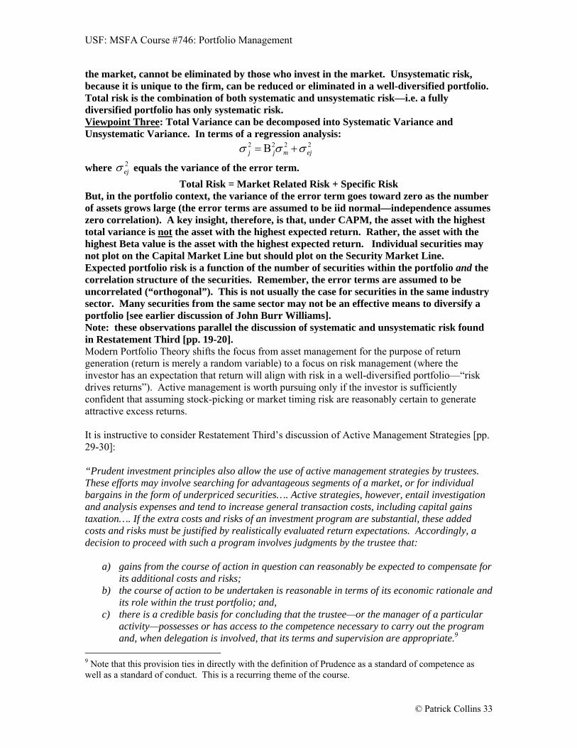
USF: MSFA Course #746: Portfolio Management
© Patrick Collins 33
the market, cannot be eliminated by those who invest in the market. Unsystematic risk, because it is unique to the firm, can be reduced or eliminated in a well-diversified portfolio. Total risk is the combination of both systematic and unsystematic risk—i.e. a fully diversified portfolio has only systematic risk. Viewpoint Three: Total Variance can be decomposed into Systematic Variance and Unsystematic Variance. In terms of a regression analysis:
2222ejmjj
where 2ej equals the variance of the error term.
Total Risk = Market Related Risk + Specific Risk But, in the portfolio context, the variance of the error term goes toward zero as the number of assets grows large (the error terms are assumed to be iid normal—independence assumes zero correlation). A key insight, therefore, is that, under CAPM, the asset with the highest total variance is not the asset with the highest expected return. Rather, the asset with the highest Beta value is the asset with the highest expected return. Individual securities may not plot on the Capital Market Line but should plot on the Security Market Line. Expected portfolio risk is a function of the number of securities within the portfolio and the correlation structure of the securities. Remember, the error terms are assumed to be uncorrelated (“orthogonal”). This is not usually the case for securities in the same industry sector. Many securities from the same sector may not be an effective means to diversify a portfolio [see earlier discussion of John Burr Williams]. Note: these observations parallel the discussion of systematic and unsystematic risk found in Restatement Third [pp. 19-20]. Modern Portfolio Theory shifts the focus from asset management for the purpose of return generation (return is merely a random variable) to a focus on risk management (where the investor has an expectation that return will align with risk in a well-diversified portfolio—“risk drives returns”). Active management is worth pursuing only if the investor is sufficiently confident that assuming stock-picking or market timing risk are reasonably certain to generate attractive excess returns. It is instructive to consider Restatement Third’s discussion of Active Management Strategies [pp. 29-30]: “Prudent investment principles also allow the use of active management strategies by trustees. These efforts may involve searching for advantageous segments of a market, or for individual bargains in the form of underpriced securities…. Active strategies, however, entail investigation and analysis expenses and tend to increase general transaction costs, including capital gains taxation…. If the extra costs and risks of an investment program are substantial, these added costs and risks must be justified by realistically evaluated return expectations. Accordingly, a decision to proceed with such a program involves judgments by the trustee that:
a) gains from the course of action in question can reasonably be expected to compensate for its additional costs and risks;
b) the course of action to be undertaken is reasonable in terms of its economic rationale and its role within the trust portfolio; and,
c) there is a credible basis for concluding that the trustee—or the manager of a particular activity—possesses or has access to the competence necessary to carry out the program and, when delegation is involved, that its terms and supervision are appropriate.9
9 Note that this provision ties in directly with the definition of Prudence as a standard of competence as well as a standard of conduct. This is a recurring theme of the course.

USF: MSFA Course #746: Portfolio Management
© Patrick Collins 34
In addition, the course of action and the overall strategy of which it is a part must be suitable to the particular trust in light of its objectives, risk tolerance, liquidity requirements, and other circumstances.” Is the portfolio manager designing investment strategies and building portfolios for the client; or, is the client hitching on to a portfolio manager that generates attractive returns by following his or her own agendas?

USF: MSFA Course #746: Portfolio Management
© Patrick Collins 35
Appendix I: Legal List: An Example from the State of Maryland Estates and Trusts Annotated Code §15-106 OPTIONAL READING—THIS MATERIAL WILL NOT BE TESTED
(b) List of lawful investments—The following investments shall be lawful investments for any person [acting in a fiduciary capacity]:
(1) Debentures issued by federal intermediate credit banks or by banks for
cooperatives; (2) Bonds issued by federal land banks or by the Federal Home Loan Bank Board; (3) Mortgages, bonds, or notes secured by a mortgage or deed of trust, or debentures
issued by the Federal Housing Administration; (4) Obligations of national mortgage associations; (5) Shares, free-share accounts, certificates of deposit, or investment certificates of
any insured financial institution….; (6) Bonds or other obligations issued by a housing authority … or issued by any
public housing authority or agency in the United States, when such bonds or other obligations are secured by a pledge of annual contributions to be paid by the United States or any agency of the United States;
(7) Obligations issued or guaranteed by the International Bank for Reconstruction and Development;
(8) Obligations issued or guaranteed by the African Development Bank; or (9) United States government obligations, whether invested in directly, or in the
form of securities of, or other interests in, any open-end or closed-end management type investment company or investment trust registered under the provisions of the federal Investment Company Act of 1940, 15 U.S.C. §80a-1 et seq., if:
(i) The portfolio of the open-end or closed-end management type investment company or investment trust is limited to direct obligations of the United States government and to repurchase agreements fully collateralized by United States government obligations; and
(ii) The open-end or closed-end management type investment company or investment trust takes delivery of that collateral, either directly or through an authorized custodian.
Note: The Maryland legal list does not prohibit the trustee from investing in assets other than those enumerated in the statute. However, there may be “a presumption against their propriety” (Restatement 3rd). Nor is the legal list a safe harbor. The trustee must still assemble a portfolio that discharges the duties of loyalty, impartiality, use of care, skill & caution, etc.

USF: MSFA Course #746: Portfolio Management
© Patrick Collins 36
Section Two: Investment Policy for Institutional Investors: Private Trusts / Foundations & Endowments / Insurance Companies / Banks Section Two continues the discussion of The Prudent Investor Rule with special attention to defining the meaning of ‘Prudence’ with respect to the management of institutional investment portfolios. Although the primary reading for this section [“Managing Institutional Investor Portfolios”] begins with a lengthy discussion of Tax-Qualified Retirement Savings Plans (e.g., Pensions and Profit Sharing/401(k) Plans), we will defer an in-depth discussion of these plans until next session. I. Towards a Modern Definition of Prudence On a preliminary basis, prudence is a credible process to enhance the probability of a successful financial outcome at a level of risk appropriate for the purposes, terms, distribution requirements and other circumstances of the trust. A well-known characterization of prudence, outlined by Bevis Longstreth (former chairman of the SEC) in 1986, is as follows [emphasis added]: “In light of the overreaching principle, reaffirmed by most soundly reasoned cases and recent legislative and administrative developments, that prudence is a test of conduct and not performance, the most promising vehicle for accomplishing that shift is a paradigm of prudence based above all on process. Neither the overall performance of the portfolio nor the performance of individual investments should be viewed as central to the inquiry. Prudence should be measured principally by the process through which investment strategies and tactics are developed, adopted, implemented, and monitored. Prudence is demonstrated by the process through which risk is managed rather than by the labeling of specific investments risks as either prudent or imprudent. Investment products and techniques are essentially neutral; none should be classified prudent or imprudent per se.” Longstreth continues: ‘…the test of prudence is the care, diligence, and skill demonstrated by the fiduciary in considering all relevant factors bearing on an investment decision. Among the relevant factors to be considered [is]…the competence of the fiduciary or the delegates selected by him to employ the product or technique.” Throughout Restatement Third, the phrase “required degree of care, skill, and caution” becomes a defining expression for prudence. ‘Competence’ or ‘skill’ in asset management is a necessary prelude to Prudence. If the goal of the process is to enhance the probability of a successful financial outcome, the asset management process must reflect a test of conduct where conduct can be defined in terms of the methods by which a fiduciary determines that its investment strategies and elections are well

USF: MSFA Course #746: Portfolio Management
© Patrick Collins 37
suited to the trust.10 The Longstreth definition also strongly suggests the importance of a standard of competence; and it would be difficult to argue that phraseology suggesting that prudence is demonstrated by the process through which strategies are developed, portfolios are implemented and monitored, and risk is managed does not implicitly assume trustee expertise in these areas. Prudence involves a credible process (conduct) as well as a requisite degree of care, skill and caution (competence).
II. Other Aspects of the Prudent Investor Rule In this section, you are introduced to several concepts that are critical for management of institutional portfolios. Test of Conduct not of Performance: or, “The Fiduciary cannot always be right; however the Fiduciary can always be Prudent” Restatement 3rd: “The trustee’s compliance with these fiduciary standards is to be judged as of the time the investment decision in question was made, not with the benefit of hindsight or by taking account of developments that occurred after the time of a decision to make, retain, or sell an investment. The question of whether a breach of trust has occurred turns on the prudence of the trustee’s conduct, not on the eventual results of investment decisions.” You will recognize that this statement is a primary underlying rationale for the establishment of a well-written Investment Policy Statement. Without an IPS, the fiduciary’s asset management strategies can only be judged according to their outcomes. The outcome of an investment in a risky asset, however, is a random variable the future value of which cannot be known at the time of making the investment. NOTE: This is a primary justification for managing assets under a written Investment Policy Statement. The IPS documents the prudence of the asset management process. Care Skill & Caution The fiduciary must exercise “care, skill and caution” in order to assure that the asset management strategy is prudent and suitable. If “care” can be defined as extensive consideration before committing trust assets to a particular course of action; if “skill” can be defined as expertise in financial economics and the statistical and quantitative methods underlying Modern Portfolio Theory; and if “caution” can be defined as an unbiased and critical examination of the likely monetary effects of asset management decisions, then the fiduciary (or the agents of the fiduciary) must demonstrate competency in these areas. This topic will be explored further in Course Sections Five and Six [Portfolio Monitoring and Evaluating Portfolio Performance]. Principles of Prudence (Restatement 3rd) 10 Note that the phrase “enhance the probability of a successful financial outcome,” differs from “maximize portfolio return,” or “beat the market.”

USF: MSFA Course #746: Portfolio Management
© Patrick Collins 38
1. Sound diversification is fundamental to risk management and is therefore ordinarily required of trustees;
2. Risk and return are so directly related that trustees have a duty to analyze and make conscious decisions concerning the levels of risk appropriate to the purposes, distribution requirements, and other circumstances of the trusts they administer;
3. Trustees have a duty to avoid fees, transaction costs and other expenses that are not justified by needs and realistic objectives of the trust’s investment program;
4. The fiduciary duty of impartiality requires a balancing of the elements of return between production of current income and the protection of purchasing power; and,
5. Trustees may have a duty as well as having the authority to delegate as prudent investors would.
Each of these principles forms a recurring theme within this course. Here are a series of preliminary questions/issues/and observations regarding each. These items merit your careful consideration both for class discussions and for final exam purposes. Diversification: Why would you want to diversify if you have good forecasting / stock-valuation skills? When is it prudent not to diversify? How does the diversification requirement of ERISA differ from the principle of diversification embodied in Restatement Third? How many securities do you need to diversify a portfolio adequately? Risk & Return: Throughout the course readings, the CFA curriculum stresses the importance of understanding the following two concepts: (1) Required Return vs. Desired Return; (2) Willingness to assume Risk vs. Ability to assume Risk. Is the risk of a portfolio controlled by picking “good” (i.e., undervalued) securities? Should fiduciaries wish to beat-the market? Should fiduciaries wish to match-the-market (indexed investing)? What risks and returns are appropriate for the fiduciary to consider and to target? What type of quantitative process constitutes making “conscious decisions concerning the levels of risk appropriate to the purposes, distribution requirements, and other circumstances of the trust?” How would such a process differ from a process based on “intention,” or “good faith?” Unjustified Costs: Are fiduciaries required to select the lowest cost products and services? How important is cost control for realizing investment success? What strategies are appropriate for cost effective securities trading? Are “soft dollars” and “directed trading” arrangements breaches of fiduciary duties? Duty of Impartiality: This is one of the most important justifications for designing and implementing sound Investment Policy. In almost every institutional portfolio management engagement there will be competing interests that are difficult to reconcile. For example, in family trusts, the interests of the income beneficiaries compete with the interests of the remainder beneficiaries (income v. growth—see section below entitled “Duty of Loyalty and The Investment Policy Statement.”). What are the competing interests in Endowment portfolio management? In Pension Plan portfolio management? In Bank securities portfolio management? In Life Insurance Company portfolio management? How does written Investment Policy mitigate or reconcile competing interests? Delegation: Which tasks should the Trustee undertake personally and which should be delegated? For asset management, what are the implications of a trustee (such as a bank) using proprietary products [see Duty of Loyalty below]? If a trustee selects an outside investment manager, what should the search process look like? How should the prospective manager be evaluated [topics for course Section Six]?

USF: MSFA Course #746: Portfolio Management
© Patrick Collins 39
Duty of Loyalty The classic definition of the duty of loyalty comes from Judge Cardozo’s decision in the 1928 case of Meinhard v. Salmon: “Many forms of conduct permissible in a workaday world for those acting at arm’s length, are forbidden to those bound by fiduciary ties. A trustee is held to something stricter than the morals of the market place. Not honesty alone, but the punctilio of an honor the most sensitive, is then the standard of behavior. As to this there has developed a tradition that is unbending and inveterate. Uncompromising rigidity has been the attitude of courts of equity when petitioned to undermine the rule of undivided loyalty by the ‘disintegrating erosion’ of particular exceptions. Only thus has the level of conduct for fiduciaries been kept at a level higher than that trodden by the crowd.” Query: Do you see how this language refers to the Section One discussions about (1) the difference between agency law and fiduciary law; and, (2) legal ownership vs. equitable interest? Note: the California Prudent Investor Statute expresses the duty of loyalty as follows: “a trustee has a duty not to use or deal with the trust property for his own profit, or for any other purpose unconnected with the trust, in any manner.”11 Duty of Loyalty and the Investment Policy Statement A written Investment Policy Statement [IPS] serves several functions with respect to prudent asset administration. In part, the IPS:
1. Documents the prudence of the trustee’s decision making process;
2. Memorializes the guidelines under which the investments will selected, monitored, and evaluated; and
3. Communicates important investment strategies (asset allocation, distribution policies, active v. passive elections for generation of investment returns, etc.) to all interested parties.
For private or family trusts, one of the most daunting challenges faced by the trustee is the balance of competing interests for various beneficiary classes. Many trusts have at least two types of beneficiaries: (1) current beneficiaries who are entitled to receive distributions of income from the trust during their lifetime(s); and, (2) remainder beneficiaries [remaindermen] who are entitled to receive a distribution of the remaining value of the trust following the death of the last member of the current beneficiary class (e.g., kids get what’s left after mom lives on the income produced by assets put into trust following dad’s death). The tension between current and remainder beneficiaries can be especially acute when there are children /step-mother or step-father relationships.
11 A current legal issue in the U.S. is the extent to which disclosure of conflicts of interest is sufficient to mitigate trustee liability. For example, if a broker/dealer-affiliated trust company provides disclosure of potential conflicts of interest, are they then free to pursue transactions (e.g., sale of proprietary products / directed brokerage arrangements, etc.), which may be otherwise categorized as self-dealing?

USF: MSFA Course #746: Portfolio Management
© Patrick Collins 40
Tension between competing beneficiary classes is also evident in many other types of trusts. Consider some of the competing interests in the management of tax qualified retirement plans. The interests of pre-retirement participants may not coincide with that of post retirement participants; or, there may be potential conflicts between a company owner/shareholder who sits on the plan’s administrative committee and the plan’s non-owner participants. The shareholder, although inclined to balance the interests of owners and workers, must make all decisions solely for the benefit of plan participants and beneficiaries. Competing interests is analogous to the mathematical problem of “Dimensionality” (problems become difficult to solve as the number of variables increase)—that is, the number of interested parties becomes so numerous that it is difficult to maintain strict impartiality. Additionally, in most every institutional investment program, a key interested party is the state or federal regulatory agency that has oversight responsibilities. One of the advantages of a written IPS is that it assists the trustee to walk the tightrope between the competing interests of interested parties. The trustee can shape the IPS in such a way that it provides solid evidence that the trustee followed well designed and clearly communicated procedures. This stands in contrast to a possible ad hoc decision-making process that may leave the trustee vulnerable to surcharge actions for breach of fiduciary duties. In drafting an IPS, therefore, it is especially important that the investment advisor have a strong grasp of:
The nature and scope of trustee duties as enumerated under common law (Restatement 3rd) as well as under applicable statutes;
The “political” or “competing-interests” nature of the asset management engagement; and,
The regulatory environment in which the engagement unfolds.
III. Charitable Trusts / Endowments Restatement Third: §379 [1990] The Duties of the Trustee “The duties of the trustee of a charitable trust are similar to the duties of the trustee of a private trust.” Restatement Third: §389 [1990] Investments of Charitable Trusts “In making decisions and taking actions with respect to the investment of trust funds, the trustee of a charitable trust is under a duty similar to that of the trustee of a private trust.” A foundation is a nongovernmental, nonprofit organization with its own funds (usually from a single source, either an individual, family, or corporation) and program managed by its own trustees and directors, which was established to maintain or aid educational, social, charitable, religious, or other activities serving the common welfare primarily by making grants to other nonprofit organizations. [David F. Freeman, The Handbook on Private Foundations, p.2]. Private Foundations Private Foundations are usually characterized by a single family or corporate funding source (e.g., the Pew Foundation, the Getty Foundation, the Hughes Foundation, and the T. Rowe Price Foundation). Private Foundations are required by the U.S. tax code to distribute 5% of the value of their assets each year or they may be subject to income tax on

USF: MSFA Course #746: Portfolio Management
© Patrick Collins 41
the undistributed amounts.12 The article in the CFA course book entitled “Managing Institutional Investor Portfolios” distinguishes four types of private foundations: Independent Foundation or Private Nonoperating or Grantmaking Foundation. Investment income of a private nonoperating foundation is currently taxed at a rate of 1% provided that minimum distribution requirements are met. A key point with respect to IPS drafting is that the advisor must recognize that these foundations are subject to minimum payout requirements. Operating Foundation. This is a private foundation that conducts its own charitable programs as opposed to making grants to other charitable organizations. Operating Foundations must utilize 85% of investment income for the active conduct of their charitable programs. Corporate or Company-Sponsored Foundation. These are company-sponsored foundations that have spending requirements similar to those of the Independent Foundation. As the name implies, a single corporation is usually the sole source of funds. Community Foundation. Organized as organizations that make grants to public charities (see below). Donors receive the maximum allowable annual tax deductions (allowable percentage of Adjusted Gross Income for individual donors) for contributions made to eligible community foundations. Note: The U.S. Tax Code divides charitable organizations into private foundations and public charities. The Revenue Service typically classifies every charitable organization as a private foundation unless the nonprofit organization specifically requests a classification as a public charity. A Public Charity is, in general, a nonprofit organization that (a) has broad public support [relies on contributions from the general public and the contributions are tax-deductible according to applicable rules and limitations]; (b) actively functions to support other public charities (i.e., a public charity like United Way can act like a private foundation), or (c) is devoted exclusively to testing for public safety purposes. Private Foundations are all remaining charitable organizations that do not qualify as public charities. Usually, they are nonprofit organizations established with funds from a single source (private family or corporate wealth). Many larger private foundations have endowments (see below). The IRS distinguishes between:
a private non-operating foundation that makes grants to other charitable organizations; and,
a private operating foundation that distributes funds to its own programs. These programs must be deemed to exist for legitimate charitable purposes—political lobbying efforts, for example, are not permitted.
Endowments The terms ‘Foundation’ and ‘Endowment’ are often used interchangeably. However, endowments are organizations specifically excepted from the Internal Revenue Code’s private foundation classification. These excepted organizations are organized under IRC §509(a)(1) and §501(c)(3) and are termed, in the Code, “public charities.” These are principally schools, churches, and hospitals. In general, there are two types of endowments: True Endowments. A true endowment is created by a gift or bequest when a donor instructs the fiduciary that the corpus of the gift be held in perpetuity (or for a specified term of years) with the income used to support the institution or a particular program. Quasi-Endowments. A fund functioning as an endowment (FFE), also called a quasi-endowment, may be created by a gift or bequest when a donor does not instruct either that
12 Note that his acts as a de facto distribution policy.

USF: MSFA Course #746: Portfolio Management
© Patrick Collins 42
the gift be expended in its entirety or held as a true endowment. In such cases, the institution may, acting in its own discretion, decide to create a fund functioning as an endowment, which means the funds are invested in the same manner as if they were subject to the terms of a true endowment, with the crucial distinction that the institution may at any time decide to withdraw all or part of the corpus of the fund and expend it for the purpose designated by the donor. Historically, courts were uncertain regarding the applicable standards of prudence to apply to charitable organizations. Sometimes, the application of law was merely a function of the organization’s name—charities organized as trusts had trust law standards applied to trustee actions; charities organized as corporations had corporate ‘business judgment rule’ standards applied to directors. The authors of the famous 1969 Ford Foundation report state “A trustee may be liable for actual negligence, but [corporate] directors have not even been held to that standard. As a practical matter courts require proof of bad faith or gross or willful neglect before imposing personal liability upon directors of business corporations, and the little authority in point indicates that this is true also in respect of directors of charitable corporations.” NOTE: market pressures are often sufficient to act as a restraint on improper corporate behavior. The guilty parties may suffer a reduction in the value of their stock/compensation packages, or may be removed by shareholder actions. There are few comparable checks on the actions of Charitable Corporations. Charitable organizations are governed by a mishmash of rules and regulations that may shape or, depending on your point of view, impinge upon portfolio investment activities. These include requirements listed in the IRC (especially code section 4944 forbidding private foundations to invest “any amount in such a manner as to jeopardize the carrying out of any of its exempt purposes;” and, state regulations (charitable corporations are subject to state Department of Corporation regulations as well as the state statutes adopting the 1972 provisions of the Uniform Management of Institutional Funds Act (UMIFA). The following paragraphs give you a “taste” of federal and state rules and governing regulations for California non-profit organizations. These rules are too complex to commit to memory—simply keep alert for changes in language from item to item. Do the rules contradict each other? What are the issues for drafting and following Investment Policy? If you were asked to become a member of a charitable organization’s board of directors, what questions would you ask the portfolio manager? Would you manage a foundation’s portfolio differently from an endowment portfolio? You can see the evolution of the law by contrasting the former California UMIFA statute (Probate Code Section 18500-18509, adopted in 1973) with the new California Uniform Prudent Management of Institutional Funds Act UPMIFA adopted in 2008 and effective starting in 2009. The former statute stated: “The [Charity’s] governing board may appropriate for expenditure for the uses and purposes for which an endowment fund is established so much of the net appreciation, realized and unrealized, in the fair value of the assets of an endowment fund over the historic dollar value of the fund as is prudent under the standard established by Section 18506.” “Historic dollar value” means the aggregate fair value in dollars of (1) an endowment fund at the time it became an endowment fund, (2) each subsequent donation to the endowment fund at the time it is made, and (3) each accumulation made pursuant to a direction in the applicable gift instrument at the time the accumulation is added to the endowment fund.” The new (2009) UPMIFA13 states:
13 §18504(a) Calif. Probate Code. Note, however, §18504(d): The appropriation for expenditure in any year of an amount greater than 7 percent of the fair market
value of an endowment fund, calculated on the basis of market values determined at least quarterly and averaged over a period of not less than three years
immediately preceding the year in which the appropriation for expenditure is made, creates a rebuttable presumption of imprudence.

USF: MSFA Course #746: Portfolio Management
© Patrick Collins 43
Subject to the intent of a donor expressed in the gift instrument, an institution may appropriate for expenditure or accumulate so much of an endowment fund as the institution determines is prudent for the uses, benefits, purposes, and duration for which the endowment fund is established. Unless stated otherwise in the gift instrument, the assets in an endowment fund are donor-restricted assets until appropriated for expenditure by the institution. In making a determination to appropriate or accumulate, the institution shall act in good faith, with the care that an ordinarily prudent person in a like position would exercise under similar circumstances, and shall consider, if relevant, all of the following factors: (1) The duration and preservation of the endowment fund. (2) The purposes of the institution and the endowment fund. (3) General economic conditions. (4) The possible effect of inflation or deflation. (5) The expected total return from income and the appreciation of investments. (6) Other resources of the institution. (7) The investment policy of the institution. NOTE: This statute assumes the existence of an investment policy. The historical restrictions on endowment fund spending are being relaxed under the new prudent investor standards. Federal regulation interpreting 4944 [Reg. 53.4944-1(a)(2)(i)] states: “…the foundation managers must exercise ordinary business care and prudence, under the facts and circumstances prevailing at the time of making the investment, in providing for the long-and short-term financial needs of the foundation to carry out its exempt purposes. Foundation managers may take into account the expected return (including both income and appreciation of capital), the risks of rising and falling price levels, and the need for diversification, within the investment portfolio. The determination whether the investment of a particular amount jeopardizes the carrying out the exempt purposes of a foundation shall be made on an investment by investment basis, in each case taking into account the foundation’s portfolio as a whole. No category of investments shall be treated as a per se violation of section 4944.” Section 18503 of the California Probate Code states: (a) Subject to the intent of a donor expressed in a gift instrument, an institution, in managing and investing an institutional fund, shall consider the charitable purposes of the institution and the purposes of the institutional fund. (b) In addition to complying with the duty of loyalty imposed by law other than this part, each person responsible for managing and investing an institutional fund shall manage and invest the fund in good faith and with the care an ordinarily prudent person in a like position would exercise under similar circumstances. (c) In managing and investing an institutional fund, an institution is subject to both of the following: (1) It may incur only costs that are appropriate and reasonable in relation to the assets, the purposes of the institution, and the skills available to the institution. (2) It shall make a reasonable effort to verify facts relevant to the management and investment of the fund. (d) An institution may pool two or more institutional funds for purposes of management and investment. (e) Except as otherwise provided by a gift instrument, the following rules apply:

USF: MSFA Course #746: Portfolio Management
© Patrick Collins 44
(1) In managing and investing an institutional fund, all of the following factors, if relevant, must be considered: (A) General economic conditions. (B) The possible effect of inflation or deflation. (C) The expected tax consequences, if any, of investment decisions or strategies. (D) The role that each investment or course of action plays within the overall investment portfolio of the fund. (E) The expected total return from income and the appreciation of investments. (F) Other resources of the institution. (G) The needs of the institution and the fund to make distributions and to preserve capital. (H) An asset's special relationship or special value, if any, to the charitable purposes of the institution. (2) Management and investment decisions about an individual asset must be made not in isolation but rather in the context of the institutional fund's portfolio of investments as a whole and as a part of an overall investment strategy having risk and return objectives reasonably suited to the fund and to the institution. (3) Except as otherwise provided by law other than this part, an institution may invest in any kind of property or type of investment consistent with this section. (4) An institution shall diversify the investments of an institutional fund unless the institution reasonably determines that, because of special circumstances, the purposes of the fund are better served without diversification. (5) Within a reasonable time after receiving property, an institution shall make and carry out decisions concerning the retention or disposition of the property or to rebalance a portfolio, in order to bring the institutional fund into compliance with the purposes, terms, and distribution requirements of the institution as necessary to meet other circumstances of the institution and the requirements of this part. (6) A person that has special skills or expertise, or is selected in reliance upon the person's representation that the person has special skills or expertise, has a duty to use those skills or that expertise in managing and investing institutional funds. (f) Nothing in this section alters the duties and liabilities of a director of a nonprofit public benefit corporation under Section 5240 of the Corporations Code. Note: The statute provides a good blueprint for the drafting of a written IPS. Unfortunately, the California Probate Code is not fully consistent with the California Corporations Code. The Corporations Code provides that, when making investments, the board must “avoid speculation, looking instead to the permanent disposition of the funds, considering the probable income, as well as the probable safety of funds.” Note: This is a standard akin to the ‘legal list.’ It reflects much common law of trusts [“The Prudent Man Rule”] prior to the adoption of Restatement Third [‘The Prudent Investor Rule”]. FASB 124 requires that distributions from the endowment as well as losses suffered by the endowment, be taken from the unrestricted asset class (FFE). The reported value of the ‘true endowment’ remains as the sum of the value of gifts and bequests on their date of transfer. All gains, losses, income, and distributions impact the FFE or unrestricted asset class. Key Concepts:
UMIFA permits a change in the traditional law of trusts that specifies that trustees could only spend current income.
The change in spending rules creates a focus on the management of a “total return” trust rather than on a “net income” trust.

USF: MSFA Course #746: Portfolio Management
© Patrick Collins 45
Under UMIFA, traditional prohibitions against delegation of investment responsibilities are repealed.
To a donor, an endowment is a fund of money given for charitable purposes; to an accountant, it is a fund of money that is “permanently restricted;” to a lawyer, it is a fund of money that is organized under the terms of a gift or governing instrument.14 As an investment manager, your job is to satisfy all parties while upholding the highest fiduciary standards!
IV. A Preface to Investment Policy for Institutional Portfolios: Utility, Asset Allocation, and Modern Portfolio Theory This section is both a brief review of basic capital market theory as well as an introduction to material that is important for a clear understanding of multi period asset management under the presence of cash flows. Investor Utility UTILITY OF WEALTH: This is a measure of “satisfaction” with any given level of wealth. As wealth changes, the investor’s satisfaction also will change with a decrease in wealth generating “disutility” and an increase generating positive “utility.” The rate of each investor’s unique utility increase or decrease can be represented by a curve graphed in wealth (x-axis) / utility (y-axis) space. For most investors the pain of losing a dollar is greater than the pleasure of gaining a dollar; and the lower the level of wealth, the more the pleasure/pain tradeoff is magnified. As wealth approaches a subsistence level, the pain of further loss may become intolerable. One important consequence of this observation is that utility is not necessarily “money-equivalent.” A dollar is merely a dollar (the unit measurement stays constant), while the amount of pleasure and pain are variables. Investors generally prefer a risk-free payoff to a risky payoff with an equivalent expected value. This is because the risk-free payoff is certain; while the risky payoff may yield an amount greater or lesser than that guaranteed by the risk-free alternative. Given that the pleasure of gain is less than the pain of an equivalent loss, a risky payoff must provide a risk-premium to induce the investor to make the investment. Thus, any payoff must be adjusted to reflect the degree of uncertainty—this adjustment yields a money-equivalent index of satisfaction. For many financial economists, utility measurement is the best way to make such an adjustment. Investor sensitivity to wealth changes is the slope value that determines the investor’s utility function curve—the rate at which wealth gains provide increased satisfaction and wealth losses generate disutility. The existence of fixed commitments alters the asset allocation preferences of many investors. Such commitments may include home mortgages (home foreclosure creates significant disutility), education costs, closely hold business obligations, and, most importantly, a threshold standard of living where the threshold is variously defined as either a subsistence level or preservation of an existing lifestyle. If the return realizations achieved under the investor’s asset management election are unfavorable—i.e., increase the likelihood of a failure to fund threshold commitments—an increasingly convex utility penalty may significantly alter the investor’s risk tolerance.
14 You will recognize the importance of an IPS as a way of integrating the various points of view.

USF: MSFA Course #746: Portfolio Management
© Patrick Collins 46
RISK AVERSION: This is a mathematical expression of the investor’s attitude towards risk. It is measured by the amount of risk premium required by the investor to make the utility of a risky asset position equivalent to that of a risk-free investment. Risk aversion curves are also known as “indifference curves.” The curve plots the series of increasingly risky investments that provide equal utility to the investor (hence, the term “indifference”). The more sensitive the investor to a change in wealth, the steeper the slope of the indifference curve—that is to say, the greater the risk premium required to induce the investor away from the risk-free “neighborhood.” The steepness of the risk aversion curve is mathematically equivalent to the change (“elasticity”) of marginal utility at any given wealth level. Investors exhibiting Absolute Risk Aversion will not risk more than a specific dollar amount on any uncertain venture; investors exhibiting Constant Relative Risk Aversion will not risk more than a specific fraction of their wealth on any uncertain venture. Relative Risk Aversion is, at least theoretically, independent of the actual level of an investor’s wealth. Given that the utility of wealth curves are generally upward slopping--at a decreasing rate of acceleration as wealth grows larger-- it follows mathematically that the upwardly sloping curves have a positive “velocity” and a negative “acceleration.” For students familiar with calculus, the curves have a positive first derivative and a negative second derivative. Although each investor has a unique attitude towards risk [and, therefore, will differ in their preferred risk/reward tradeoffs], it is generally true that the risk aversion function is expressed as follows:
Risk Aversion = -(second derivative of the utility of wealth) ÷ +(first derivative of the utility of wealth).
In other words, an investor’s risk aversion function can be derived from the shape of the individual’s utility of wealth curve; and the investor’s utility of wealth can be recovered from his risk aversion curve. There is a substantial literature on fitting specific risk aversion functions to investor preferences. Each risk aversion function curve has a unique slope (rate of change) reflecting the individual investor’s sensitivity to changes in wealth. It is common to build risk aversion curves that are (1) quadratic (an upside-down bowl shape); (2) exponential (increasing exponential risk aversion where the exponent is a negative fraction); (3) power (where the exponent ranges from a value greater than 0 through to a value of 1); and, (4) logarithmic (where the value of the exponent approaches 0). Although many modifications (called “positive affine transformations”) are possible for each of the common forms of risk aversion curves, a simple way to gain an intuitive understanding is to compare the “risk premium” required by investors where the probability of loss is equal to the probability of gain (e.g., odds = 50/50). We assume that the hypothetical investor has a current wealth endowment of $1 million. The investor with quadratic risk aversion (curve = square root of wealth) requires a
payoff of at least $51,282 to risk a loss of $50,000;
The investor with a power risk aversion exponent of 0.1 requires a payoff of at least $52,356 to risk a loss of $50,000; and,
The investor with logarithmic risk aversion requires a payoff of at least $52,632 to risk a loss of $50,000.
The payoff (asset allocation risk/reward tradeoff) that will satisfy one investor is unsatisfactory to other investors. How do we know how much dollar gain must be put on the table to risk the $50,000 loss? For the quadratic risk-averse investor, the square root of $1,000,000 equals 1,000. That is

USF: MSFA Course #746: Portfolio Management
© Patrick Collins 47
to say, $1,000,000 generates 1,000 units of utility. By risking $50,000, the investor may increase wealth to $1,051,282 or decrease wealth to $950,000. But the square root of $1,051,282 is 1,025.32; and the square root of $950,000 is 974.68. Thus, at 50/50 odds, the average of the two risky gamble square roots equals 1,000 units of utility which is the exact value of the risk free $1,000,000. If wealth decreases towards a critical level, the slope of the investor’s indifference curve may become steeper. Similar mathematical calculations confirm the values for the power risk aversion (exponent of 0.1) and the log of wealth risk aversion function. RISK TOLERANCE: This is the reciprocal of the risk aversion function curve [1 ÷ Risk Aversion]. The less risk averse; the more risk tolerant. Asset Allocation and Investor Utility You remember that the Markowitz algorithm for solving the portfolio selection problem (i.e., finding the optimal portfolio) under conditions of uncertainty (i.e., risky assets only) requires three inputs:
1. Expected Return
2. Expected Variance of Return
3. Correlation Structure of Securities
The variance of a two-asset portfolio when the value of the correlation statistic equals +1 (i.e., perfect correlation) is defined as:
2p = (WAA + WBB)2
NOTE: This is a perfect square.
However, when the value of the correlation statistic is less that +1 (with a lower boundary equal to –1), then the equality sign becomes an inequality:
2p < (WAA + WBB)2
If the distribution of risky asset returns is approximately (log)normal, then only its first two moments (mean and variance) are needed to fully describe it. That is to say, only first and second order (i.e., squared) terms are relevant to the investment decision. [Note: there are several extensions of Markowitz that involve higher order terms such as skew and kurtosis]. The assertion that the Markowitz portfolio selection process assumes that investors care only about expected means and variances is equivalent to stating that investors have quadratic utility because variance is a squared term and there are no terms of a higher order:
U(W) = expected return – ½(variance)(risk aversion parameter); or, U(W) = - ½ 2(A)
This equation indicates that investor utility of wealth U(W) increases with return and decreases with uncertainty (i.e., variance of return) with each investor having a unique risk aversion curve. The equation is a specific form of the more general equation:
Utility = a + bX – cX2
Where is expected return (a + bX) and the first derivative (marginal utility) is b - 2cX. The optimal portfolio is, according to Markowitz, the portfolio that maximizes the utility of terminal wealth in a single period planning horizon. The Markowitz algorithm is appropriate only for a “myopic” investor (i.e., not concerned about future planning periods).15
15 Technically, the Markowitz algorithm is appropriate for a multiperiod investor assuming that the distribution of returns is iid normal (investment opportunity set is constant) and that variance is finite.

USF: MSFA Course #746: Portfolio Management
© Patrick Collins 48
In terms of Utility theory, a Markowitz investor exhibits quadratic utility such that satisfaction is measured by the square root of terminal wealth. That is to say, an investor is risk averse if
E[U(W)] > U[E(W)]. For example, if Wealth (W) = $400, for quadratic utility:
E[U(W)] = U($400)= 4001/2 = 20. However, for an uncertain proposition where W = $100 at 50/50 odds or $700 at 50/50 odds, E(W) = 1002 = $50 plus $7002 = $350. Therefore E(W) = $50 + $350 = $400.
But U[E(W)] = 23.182
700
2
100
And, 20 > 18.13. Despite equal expected value, the risk-averse investor prefers the more certain outcome. NOTE: for investors with log of wealth utility, the portfolio that maximizes the compound rate of growth over the applicable planning horizon is optimal. This is because:
Terminal Compound Wealth Initial Wealth[Average Return – ½(Variance)].
NOTE: Quadratic Utility is an example of Power Utility with Wealth raised to the power of 0.5. Log utility, at the limit, approaches power utility with Wealth raised to the power of .0001. A log utility investor is more risk sensitive than an investor exhibiting quadratic utility (i.e. he or she demands a bigger payoff or better odds when placing money at risk). Conversely, an investor with power utility approaching .999 is almost linear with respect to risk. The portfolio that satisfies one investor will not be the portfolio that satisfies another simply because their utility of wealth functions differ. The “CFA readings” in the course speak about aligning desired return / required return / risk. This is a process of matching the portfolio’s payoff function to the investor’s utility function. Maximizing single period Utility is the same as implementing a portfolio that is on the highest possible feasible “indifference curve” (isoquant). In a world in which assets exhibit less than perfect correlation, achieving the most efficient portfolio means finding the combination or weighting of assets that offers the greatest reward per unit of risk and the lowest risk per unit of reward. This is an asset weighting or asset allocation decision—the weights of the assets express the investor’s decisions (and, given the Markowitz assumption that investors are rational, it would be irrational for investors to arrive at differing estimates of the algorithm’s inputs). Thus, in terms of the classic expression of the risk (standard deviation) of a portfolio:
2/12222 2 jiijjijjiiport wwww
The investment / asset allocation decision becomes the decision where to position the portfolio on the efficient frontier so that the investor maximizes his or her utility of end-of-period wealth. When the location on the frontier exactly matches the investor’s risk-aversion preferences, the portfolio resulting portfolio is the optimal portfolio.

USF: MSFA Course #746: Portfolio Management
© Patrick Collins 49
Key Concept: The Markowitz model is a “closed-form” solution to an optimization problem. The model assumes that cash flows, if any, are paid at the end of the period under evaluation. Thus, the classic Markowitz model of portfolio selection is a single-period model. For a multi-period model in the presence of cash flows [a situation more likely to be faced by institutional investors—remember that foundations, for example, have minimum periodic distribution requirements], the concept of utility must be extended to include:
1. The utility of terminal wealth,
2. The utility of interim wealth (e.g., think of a defined benefit pension that seeks to always maintain a surplus)
3. The utility of consumption (think of an endowed institution that relies on portfolio distributions to fund its operating budget).
Thus, in terms of financial economics, asset management is an activity demanding that the IPS guidelines are well aligned with all components of investor utility. This is difficult for institutional investment portfolios because of the competing objectives and financial goals of multiple interested parties. The following graphs illustrate these concepts:

USF: MSFA Course #746: Portfolio Management
© Patrick Collins 50
Constant Risk Aversion
Wealth/Consumption
Utility
Constant Risk Aversion
Marginal Wealth/Consumption
MarginalUtility
Constant Risk Aversion
Log Marginal Wealth/Consumption
Log MarginalUtility
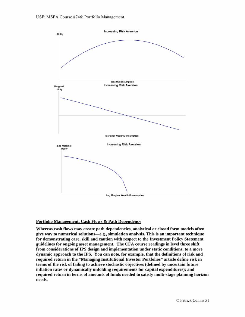
USF: MSFA Course #746: Portfolio Management
© Patrick Collins 51
Portfolio Management, Cash Flows & Path Dependency
Whereas cash flows may create path dependencies, analytical or closed form models often give way to numerical solutions—e.g., simulation analysis. This is an important technique for demonstrating care, skill and caution with respect to the Investment Policy Statement guidelines for ongoing asset management. The CFA course readings in level three shift from considerations of IPS design and implementation under static conditions, to a more dynamic approach to the IPS. You can note, for example, that the definitions of risk and required return in the “Managing Institutional Investor Portfolios” article define risk in terms of the risk of failing to achieve stochastic objectives (defined by uncertain future inflation rates or dynamically unfolding requirements for capital expenditures); and required return in terms of amounts of funds needed to satisfy multi-stage planning horizon needs.
Increasing Risk Aversion
Wealth/Consumption
Utility
Increasing Risk Aversion
Marginal Wealth/Consumption
MarginalUtility
Increasing Risk Aversion
Log Marginal Wealth/Consumption
Log MarginalUtility

USF: MSFA Course #746: Portfolio Management
© Patrick Collins 52
Here is a highly stylized example:
We know (because multiplication is commutative) that 3*2*1 = 6; and that 1*2*3 = 6. The order of the ‘returns’ does not matter. This principle holds for any compound return series in which there are no cash flows. Consider, however, what happens when we add cash-flow requirements—withdraw 1/2 unit of value—to the series:
Period One: 1*3 = 3 – ½ = 2½ *2 = 5
Period Two: 5 - ½ = 4½ * 1 = 4½
Period Three: 4½ - ½ = 4 units of ending wealth.
However,
Period One: 1*1 = 1 – ½ = ½ * 2 = 1
Period Two: 1 – ½ = ½ * 3 = 1½
Period Three: 1 ½ - ½ = 1 unit of ending wealth.
What happened? The order in which returns are earned matters when there are cash flows.16 An average return “target” is no longer sufficient in the presence of portfolio distributions and return variance. Cash flows change the definition of required return.
Two important asset management implications:
1. People Spend Dollars not Rates of Return. (The ‘Flaw of Averages’17) Over time, when faced with the presence of cash flows, one can be exactly on track with respect to a portfolio’s expected average return; but wildly off with respect to the portfolio’s actual dollar value. It is the dollar value, however, that must support financial objectives.
2. Variance decrements Wealth (‘Variance Drain’). You know that, absent cash flows, downside variance hurts a portfolio more than upside variance helps. For example, if you start with $1.00 and lose 20% in period one, you need to earn 25% in period two simply to get back to even [0.80*1.25 = $1.00]. Even worse, whenever a portfolio experiences periods of gains and losses, cash flow distributional demands act as a further decrement to dollar wealth. This is because, during periods of losses, the distributions act as multipliers (i.e., there are fewer dollars left in the portfolio to “rebound” in a period of gains).18 Conversely, during periods of gains, distributions act as a cap (the full dollar value of the portfolio cannot participate in the gain because assets must be liquidated to raise cash for distributions). Multiplying losses and capping gains cannot be good!
16 This is sometimes termed the “sequence of returns” risk. 17 Beware the flaw of averages. This is what killed the overconfident statistician who drowned while crossing a river with an average depth of only 3 feet. 18 This is also known as “feeding the bear.”

USF: MSFA Course #746: Portfolio Management
© Patrick Collins 53
Therefore, it should not come as a surprise that one important current issue in Investment Policy for Institutional Investors is the coordination of Asset Allocation with Distribution Policy. 19
Note: thus far, the course has presented several concepts of diversification. There is the “Markowitz” or classic Modern Portfolio Theory justification for diversification (mitigation of uncompensated risk); and the “ERISA” or prudent expert justification for diversification (limit the possibility of incurring a large loss). To these, we can now add the “Variance Drain” justification for diversification. The Variance Drain concept suggests that diversified portfolios can limit downside risks and, consequently, better support long-term cash withdrawals.
Query: Is more money always better than less (The “Nonsatiation Principle”)? Does the highest expected multiperiod return strategy dominate all other portfolio design alternatives? Can you create more wealth by limiting variance than by seeking greater expected return?
V. Family Trusts, Investment Policy & Restatement Third:
Consider the following passage from Restatement Third:
“Among the characteristics a trustee should consider in examining a contemplated investment are the following:
(1) Expectations concerning the investment’s total return, and also the amount and regularity of the income element of that return….
(2) The degree and nature of risks associated with the investment, and the relationship of its volatility characteristics to the diversification needs of the portfolio as a whole;
(3) The marketability of the investment, and the relation between its liquidity and volatility characteristics and the amount, timing, and certainty of the trust’s cash flow or distribution requirements;20
(4) Transaction costs (including tax costs) and special skills associated with the acquisition, holding, management, and later disposition of the particular investment; and;
(5) Any special characteristics of the investment that affect it risk-reward tradeoffs and effective return, such as exposure to unlimited tort liability, the presence and utility of tax advantages, and the maturity dates and possible redemption provisions of debt instruments.
…Asset selection also requires sensitivity to the trust’s investment time horizons and to the goals and needs of the trust.”
Key Concepts:
Note similarity to CFA Institute Standards of Practice provisions for Standard III(C) [Duties to Clients: Suitability]: “a member or candidate should take the following into consideration:
19 These topics are further developed in Section 3. Try to keep these observations in mind as you read the “Asset Allocation” article’s [§3.2 & §3.3] discussion on Return Objectives and Strategic Asset Allocation pp. 14-16 and Risk Objectives and Strategic Asset Allocation (pp. 16-19). 20 This might have special application to limited liquidity investments such as hedge funds and private equity programs.

USF: MSFA Course #746: Portfolio Management
© Patrick Collins 54
Client identification—(1) type and nature of clients and (2) the existence of separate beneficiaries, and (3) approximate portion of total client assets;
Investor objectives—(1) return objectives (income, growth in principal, maintenance of purchasing power) and (2) risk tolerance (suitability, stability of values);
Investor constraints—(1) liquidity needs, (2) expected cash flows (patterns of additions and/or withdrawals), (3) investable funds (assets and liabilities or other commitments), (4) time horizon, (5) tax considerations, (6) regulatory and legal circumstances, (7) investor preferences, prohibitions, circumstances, and unique needs, and (8) proxy voting responsibilities and guidance.”
Performance measurement benchmarks.” [p. 71—2005 Standards of Practice Handbook].
The Standards of Practice recommendations are also memorialized in Section B(6a) and B(6b) of the Asset Manager Code of Professional Conduct. Each student should know this material cold—especially the elements of a well-designed IPS and the application of each element to the needs and circumstances of the client. Query: In your opinion, is setting investment policy the same as setting a strategy for generating investment returns? VI. Formulating Investment Policy The course reading for this session asks candidates to develop a skill set sufficient to allow them to formulate an investment policy statement for a foundation, an endowment, an insurance company, and a bank. I highly recommend that each student create a series of information matrices. Each matrix can be devoted to one of the important IPS considerations [return objectives, risk tolerances, liquidity requirements, time horizons, tax considerations, legal and regulatory environment, and unique circumstances & needs]; and can fill in the appropriate information for each type of institutional client [foundation, endowment, insurance firm, and bank]. To assist you in this task, I have developed a sample matrix for a U.S. “legal and regulatory environment” [Many private trusts and charitable trusts & foundations are purely creatures of the tax code—it is not certain where tax provisions and legal provisions start or end]. Note that we have not discussed the implication of Uniform Principal & Income Acts nor Trust Code provisions. In this course, you are only responsible for knowing that these statutes contain various provisions that facilitate trust administration so that it may more comfortably conform to the Prudent Investor Rules. Section Three of this course discusses pension plans, which are included in the grid for the sake of completeness.
Institutional Client Statutes Oversight Body Other Notes & Items
Private Trusts (administered by a commercial fiduciary such as a bank trust department).
State “Uniform Acts”:
1. Prudent Investor Act
2. Principal & Income Act
3. Trust Code.
Office of Comptroller of Currency for Bank Trust Departments / Office of Thrift Supervision for Independent Trust Companies and Savings & Loans. Note—the OTS is being phased out of the government regulatory structure.
Specific trust provisions may modify or eliminate certain trustee duties. Private Trust administration must conform to all applicable tax code provisions to realize income, gift, or estate tax objectives.
Private Foundations State Uniform Management of Institutional Funds Act [UMIFA]. State Prudent Investor Act IRC §4944
State Attorney General Internal Revenue Service
Some statutes have a “prudent expert” orientation while others have a “prudent business judgment” orientation.” IRS concerned with investments jeopardizing the organization’s tax-exempt purposes. Note: minimum

USF: MSFA Course #746: Portfolio Management
© Patrick Collins 55
distribution requirement rules.
Endowments State Uniform Management of Institutional Funds Act [UMIFA]. State Prudent Investor Act
State Attorney General Internal Revenue Service
FASB 124 restrictions on distributions (only in excess of historical cost) Some statutes have a “prudent expert” orientation while others have a “prudent business judgment” orientation
Life Insurance Companies State Insurance Codes & Regulations
State Insurance Commissioner
National Association of Insurance Commissioners (NAIC) promulgates model statutes and standards. Note Risk Based Capital [RBC] requirements. Insurance companies operate under Statutory Accounting Principles [SAP not GAAP] regulations.
Banks State and Federal Banking Laws
Office of Controller of Currency for Banks / Office of Thrift Supervision for Savings & Loans.
Note bank reserving / pledging requirements and Risk Based Capital [RBC] requirements
Defined Benefit Pensions ERISA U.S. Treasury Department (especially IRS)
Plans must have actuarial certification / underfunded plans subject to insurance premium increases from Pension Benefit Guarantee Corporation [PBGC].
Defined Contribution Pensions
ERISA / DOL regulations for 401(k) Plans
U.S. Treasury Department (especially IRS) / Department of Labor (DOL)
Note special regulations for participant-directed plans [ERISA §404(c) liability exemption]
VII. Managing a Bank’s Security Portfolio The Office of the Comptroller of the Currency regulates banks. I have provided a brief excerpt from the OCC manual so that you can glimpse the nature and scope of bank regulation. The following discussion is drawn from material that used to be in the CFA curriculum; but was eliminated several years ago. Generally, the bank’s decision to purchase securities for their investment portfolio comes last in a pecking order that determines the use of bank funds. Specifically, banks utilize funds to (1) meet reserve requirements; (2) meet liquidity needs; (3) serve loan demand; and, (4) invest in securities portfolios. A fundamental problem faced by banks is that during recessionary periods when loan demand is slack and interest rates are low, the bank can invest excess funds into fixed income securities. However, as the business cycle moves from recession to growth, loan demand must often be satisfied by selling securities at a loss [WHY?]. If bank management forecasts that liquidity may be needed for the security portfolio (in order to finance the demand for loans), then funds may be directed only into the purchase of short-term instruments. By the end of the business cycle, a bank may have made commitments for a portfolio of long-term loans; but may find itself holding a portfolio of short-term debt. Thus, a well considered plan for the optimal management of the bank’s security portfolio is of great importance. Banks incur four types of risk in a portfolio of fixed income securities:
1. Marketability Risk
2. Interest Rate Risk (including reinvestment risk and prepayment risk)
3. Credit Risk or Default Risk
4. Purchasing Power Risk (which is highly correlated to interest rate risk)

USF: MSFA Course #746: Portfolio Management
© Patrick Collins 56
Additionally, some fixed income instruments have option-like characteristics because they are callable or have embedded put options. Banks have limited ability to exclude tax-favored interest payments paid by securities issued by states and municipalities (interest paid on deposited funds used to purchase these securities is tax-deductible within the limits of Tax Equity and Fiscal Responsibility Act, and the bank cannot exempt an amount equal to the average cost of the funds used to finance the purchase of the municipal securities. The Tax Reform Act of 1986 imposed additional restrictions on bank ownership of larger issues of state and local bonds. For the purposes of the course, remember that the changes in the Revenue Code have resulted either in the elimination or lowering of the tax exemption available to banks owning municipal securities). Therefore, the lower rates generally offered on munis, combined with the inability to exclude coupon payments from ordinary income, may make these instruments unattractive for bank portfolios. Managing the portfolio is a five step process:
1. Establish General Criteria and Objectives. A written investment policy for bank-owned portfolio management has two advantages: (1) it provides for a continuity of approach over time; and (2) it serves as a concrete basis for appraising portfolio performance. Objectives should be achievable, understandable and measurable.
2. Forecast Interest Rates and Economic Environment. Portfolio decisions should be consistent with the bank’s forecasts; but adequate safeguards should be in place lest the forecast proves incorrect.
3. Inventory Investment Needs, Risk Positions, Pledging Requirements, Level of Diversification, Interest Sensitivity, and Tax Position, Liquidity Needs, and Capital Position.
4. Establish Policies and Strategies focusing on the appropriate Portfolio Size (given loan demand, liquidity requirements, pledging requirements, and profitability of other opportunities such as leasing and loan generation), Risk, Maturity, and Marketability characteristics of the investment portfolio.
5. Delegate Authority for effective action and responsibility.
Bank fixed income portfolio management requires special attention to maturity policies and strategies. The (theoretically) “ideal” strategy is comparable to a market timing strategy for stocks which adjusts portfolio beta upwards at the beginning of a bull market and downwards at the start of a bear market. For fixed income instruments (bonds), such a strategy involves increasing duration just prior to a long-term decline in interest rates and decreasing or shortening duration just prior to a long-term increase in interest rates. This a cyclical maturity strategy. Unfortunately, the imperatives and constraints faced by the portfolio manager often exist in an uneasy relationship with the imperatives and constraints faced by the needs to satisfy shareholders. During periods of rising interest rates and increased loan demand (expansionary economy), there is pressure to sell long-term securities, use funds to generate loans, and, in general, keep maturities short term to satisfy high demands for portfolio liquidity. In the opposite economic environment (business contraction and low loan demand), there is pressure to use the portfolio to boost bank earnings by investing long-term (reaching for yield). The other forms of fixed income “maturity policies and strategies” are staggered or evenly spaced maturities (a maturity ladder); and a barbell maturity strategy which keeps a percentage of funds short and liquid while investing remaining funds long-term to increase yield. The former strategy is often used in smaller sized banks that lack fixed-income management expertise.

USF: MSFA Course #746: Portfolio Management
© Patrick Collins 57
VIII. Bank Investment Policy: Office of the Comptroller of the Currency [“The Role of a National Bank Director—the Director’s Book / March 1997]. “Investments traditionally have been a bank’s second largest source of income. Investments should generate quality earnings, allow the bank to diversify its asset base, and provide liquidity. While the board may seek advice from technically competent managers or external sources such as correspondent banks, brokerage houses, or consulting services, it may not delegate its responsibility for overseeing the investment portfolio. The investment policy should state that the bank must comply with legal restrictions on the types of securities it may hold. It also should specify the type and composition (including the maturity and repricing characteristics) of instruments the bank may have. Factors such as the bank’s earnings, ability to accept risk, liquidity needs, pledging requirements, funding sources, and income objectives help define the board’s policy objectives. The board should review the portfolio as necessary to confirm that the risk level remains acceptable and consistent with previously approved portfolio objectives. The review should include information on the current market value of the portfolio and consideration of whether the investment policy needs to be revised…. When considering investment portfolio activities, the following practices or conditions should trigger additional board scrutiny: Failure to select securities dealers carefully. Management should be aware of the credit standing, record, and reputation of securities dealers with whom the bank does business. The board should reaffirm a list of approved securities dealers annually to ensure that the bank does not deal with financially unstable, irresponsible, or dishonest securities dealers. Efforts to obtain higher yields without regard for other portfolio objectives. A bank should not extend the maturity of the investment portfolio to obtain higher yields without carefully considering liquidity and funding issues. Extending maturities without evaluating these issues increases liquidity and interest rate risks because unanticipated liquidity demands may lead to the sale of securities at depressed market prices. In addition, interest rate movements or changes in quality can cause the value of securities to decline. The purchase of low-quality investments to obtain higher yields. Low-quality investments are highly volatile because they can experience wide price fluctuations as interest rate or other investor expectations change. As a result, purchasing these investments increases credit risk. Lower quality investments also impair a bank’s liquidity and reduce flexibility in managing the investment portfolio. Failure to adequately diversify investments. A bank that has concentrations of investments in the securities of individual obligors or groups of obligors with common economic ties could have an unsound investment portfolio strategy because price fluctuations, a deterioration of the quality of the securities, or loss of principal will have an increased impact on the bank’s financial statement. Failure to consider pledging requirements in investment decisions. To meet present and future funding needs, a bank must be able to pledge eligible securities to support deposits of public funds and to use as collateral. When developing portfolio and liquidity strategies, management must consider the eligibility of securities to meet the bank’s pledging and repossession requirements. Failure to institute adequate internal controls for investment and trading activities. Some banks have experienced substantial losses because the internal controls on their investment and trading operations were inadequate to monitor and control risks. A bank with significant investment portfolio transactions or one engaging in trading activity should be certain that controls such as a segregation of duties are in place. Failure to ensure the investment portfolio complies with current accounting standards. Current accounting standards require a bank to divide its investment portfolio into three parts: held-to-maturity, available-for-sale, and trading. Securities in the held-to-maturity portfolio

USF: MSFA Course #746: Portfolio Management
© Patrick Collins 58
are those in which a bank has the intent and ability to hold until maturity; a bank may not use this portfolio to engage in trading or to conduct speculative securities transactions. The securities in the available-for-sale account are those that will be sold at a future date but will not be traded often enough to qualify for the trading account. The trading portfolio holds securities bought and held principally for selling in the near term; a bank must record and report trading transactions in this account.” IX. Institutional Investors and Municipal Bond Portfolios The code governing taxation of municipal bonds for institutional investors is a complicated and ever-changing set of rules. As of 2008, the deductibility of muni bond interest by banks is limited (see discussion above). Life insurance companies, in general, also incur full taxation on muni bond interest payments when muni bonds are held as an asset to fund policy reserves. As a result, few life insurers make substantial investments in muni bonds. The situation is much different for property and casualty [P&C] insurers. Historically, P&C companies have held up to 40% of their asset portfolios in muni bonds. In general, only 15% of muni bond income is considered taxable revenue by the IRS as of the end of 2008. Keep in mind, however, that there are several types of muni bonds issued by states and municipalities; and that some types of bonds generate fully taxable interest. For example, bonds that fund “private activities” such as the construction of sports stadiums may be subject to full taxation. Additionally, for both private and institutional investors, the Alternative Minimum Tax places an upper limit on the amount of tax preferenced income that the investor can receive. If the individual investor is over the AMT tax limit, then 75% of the tax-preferenced income is added to taxable income and it is taxed at a 20% rate. For P&C companies, current tax law converts any AMT payments into tax credits that are applicable in future years. Economically, this has the effect of converting AMT payments to the IRS into interest-free loans to the federal government. As the course readings suggest, the attractiveness of municipal bonds is a function of the underwriting cycle for a P&C company. During profitable years, tax preferenced income from munis can be compared to fully taxable yields from corporate bonds (assuming no discount or premium paid at purchase) in order to determine the “cross over” or “indifference” point for holding munis. Remember, determining the cross over point is a function of projected taxable profits and the AMT trigger. The portfolio manager must account for both factors when deciding to buy or sell munis. Of course, when the underwriting cycle produces losses, munis cease to be an attractive asset. Other factors to consider when managing a portfolio of muni bonds are:
1. Historical and projected default rates across the various ratings categories (Aaa, Aa, A, Baa….);
2. Duration of the bond portfolio in relation to the duration of the P&C liabilities;
3. The tax-adjusted yield curve spread (munis vs. corporate) across various bond maturities.
For example, a manager might identify a significant yield spread advantage for long-term munis, a significant default credit advantage for long-term munis; but, a short duration liability structure. The decision is, in part, whether to mismatch asset/liability duration in the hopes of picking up a substantial return advantage. You should recognize that the P&C insurance company’s underwriting profitability cycle is analogous to a bank’s loan demand cycle. Asset management strategies depend on business needs as well as on “modern portfolio theory” prescriptions.

USF: MSFA Course #746: Portfolio Management
© Patrick Collins 59
X. Previous Exam Questions Question #1: Part One: Compare and contrast asset management / investment policy issues for a Defined Benefit Pension Plan and a Life Insurance Company’s Policy Reserve Portfolio. Part Two: Consider the following facts regarding the current status of the ABC company’s defined benefit plan as well as ABC’s current financial status: (1) ABC Company consists of three separate operating divisions the eligible employees of which are covered under a defined benefit pension plan; (2) The average age of ABC’s workforce is 43; (3) The plan’s funding ratio is currently 0.90; (4) ABC plans to sell its manufacturing division in Fresno in approximately two years. The average age of the Fresno workforce is 57; (5) Starting next month, ABC plans to offer each Fresno employee an early retirement option that, if accepted, will automatically accelerate any non-vested plan benefits and will substitute their current age for the plan’s normal retirement age; (6) Although ABC has not been profitable for the past several years, the majority of losses are attributable to the Fresno division. The Plan’s Investment Committee wishes to begin a study aimed at revising the plan’s investment policy to account for the sponsor’s changed circumstances. Identify and discuss critical issues regarding the Plan’s willingness and ability to accept investment risk. Question #2: Tom Thumb, an experienced accountant, had a phone conversation with Judy, the widow of his best friend Punch who died in an automobile accident. Judy is Punch’s second wife. Prior to his death, Punch had appointed Tom as successor Trustee to his revocable “living trust.” The trust designates Judy as the income beneficiary, and Tom’s children from a former marriage as remainder beneficiaries. The trust language specifies that Judy is entitled to trust accounting income (dividends, interest, rents); and the children, upon Judy’s death are entitled to receive the trust’s remaining principal. Currently, the trust portfolio is allocated 50% to fixed income securities and 50% to equity securities. In the recent phone conversation, Judy complained bitterly about the amount of current accounting income distributions. Given a recent decline in interest rates, the fixed income portion of the trust’s investment portfolio was yielding only 3%. Moreover, following a rise in stock prices, the dividend yield on the equity portion of the portfolio was less than 2%. Tom believes that the relationship between the children and their stepmother is not good; and that the children would oppose any attempt to further tilt the portfolio’s allocation to benefit Judy. Judy is currently age 70 and in good health. Tom’s three children are in their 50s. As an experienced investment advisor, Tom has asked you to help him through this thicket of problems: Given the above facts, identify and briefly discuss a fiduciary duty that is central to
the current management issues confronting the Punch Trust portfolio; Identify and briefly discuss two planning options (other than the option to make no
portfolio changes) available to Tom. Discuss how Tom might evaluate the merits and liabilities of each of the planning
options; Do you think that Tom can arrive at an equitable solution and communicate it to
Judy and the children so that both parties will be satisfied? If ‘No,’ why; if ‘Yes,” How?

USF: MSFA Course #746: Portfolio Management
© Patrick Collins 60
Section Three: Investment Policy for Institutional Investors (Pension Plans) / Asset Allocation / Asset-Liability Management [ALM] I. ERISA §404(a)
Tax qualified retirement plan assets must be placed in a trust (i.e., cannot remain under the ownership or control of the sponsoring business entity). Retirement plan trustees are fiduciaries that invest and manage under the terms of the Employee Retirement Income Security Act [ERISA]. ERISA has been called a “Federalization of the U.S. Common Law of Trusts.” ERISA Section 404(a) governs the investment standards required of an ERISA trustee. These standards require that plan assets be invested prudently and, in general, be diversified. You will recall from Section One (history of fiduciary standards), that ERISA §404(a) states: “…a fiduciary shall discharge his duties with respect to a plan solely in the interest of the participants and beneficiaries and—
(A) for the exclusive purpose of: (i) providing benefits to participants and their beneficiaries; and (ii) defraying reasonable expenses of administering the plan;
(B) with the care, skill, prudence, and diligence under the circumstances then prevailing that a prudent man acting in a like capacity and familiar with such matters would use in the conduct of an enterprise of a like character and with like aims;
(C) by diversifying the investments of the plan so as to minimize the risk of large losses, unless under the circumstances it is clearly prudent not to do so; and
(D) in accordance with the documents and instruments governing the plan insofar as such documents and instruments are consistent with the provisions of this subchapter…..”
Recall that Session One discusses (1) elements of Prudence; (2) duties of a fiduciary; and (3) standards of conduct. If you were presented with the text of §404(a), how would you characterize the treatment of each of these items? Remember, the King v. Talbot investment standards viewed diversification as a bad idea because owning a broad cross-section of “speculative” assets subjected trust principal to the risk of loss. You will also recall the following Key Concepts from Session One:
The Prudent Expert Standard: “Thus, the investment fiduciary is held to the standard of a ‘prudent expert,’ that is, ‘of a prudent man…. familiar with such matters.’” [Howard v. Shay, 1993 US Dist. Lexis 20153, (C.D. Cal.1993)].
Investment Managers hired by the retirement plan trustees are fiduciaries: “…a person is a fiduciary with respect to a plan to the extent (i) he exercises any discretionary authority or discretionary control respecting management of such plan or exercises any authority or control respecting management or disposition of its assets, (ii) he renders investment advice for a fee or other compensation, direct or indirect, with respect to any moneys or other property of such plan, or has any authority or responsibility to do so….”
Diversification requirement for prevention of large losses rather than for enhancing portfolio efficiency (level of return at a given level of risk). Restatement Third, by contrast, calls for broad diversification both across and within asset classes.
Duty to avoid inappropriate or unnecessary costs. Historically, most U.S. tax-qualified retirement savings plans (i.e., Defined Benefit Pension Plans, Defined Contribution Pension Plans, Profit Sharing Plans, and variations thereon)

USF: MSFA Course #746: Portfolio Management
© Patrick Collins 61
have been sponsor or company directed plans established and administered under the 404(a) code provisions.21 The “Managing Institutional Investor Portfolios” article in the textbook opens with a discussion regarding the differences between corporate-sponsored Defined Benefit [DB] Plans (of which Cash Balance Plans are a subset), and Defined Contribution [DC] plans (of which Profit Sharing Plans are a subset). Although this material may seem arcane because the retirement plans are creatures of a complicated U.S. tax code, nevertheless it is basic information that should be mastered by each student. In particular, you should develop facility in discussing the liabilities inherent in sponsorship of and participation in both DB and DC plans. In a nutshell, DB plans shift investment risks (technically, the risk of a shortfall in benefit funding) to the corporate sponsor; DC plans shift investment risks (technically, the risk of insufficient retirement accumulations) to plan participants. Note: Individual Retirement Accounts [IRAs] are tax-qualified personal accounts and are not subject to ERISA. II. Defined Benefit v. Defined Contribution Retirement Savings Plans
You should be prepared to answer exam questions along the lines of “Compare and contrast the important aspects of Risk Tolerance for a Company Sponsored DB Plan and a Company Sponsored DC Plan;” or “Compare and contrast the important aspects of Risk Tolerance for a Company Directed DC Plan and a Participant Directed DC Plan.” The following is a sample comparison of certain IPS issues and inputs for Defined Benefit (DB) and Defined Contribution (DC) Pension Plans. I suggest that you create a “matrix” for each underlined category [see example in Session Two] and that you fill in the matrix with relevant information.
Risk Tolerance: DB plans commit the corporate sponsor to provide plan participants with specified current and future benefits. Plan sponsors therefore fully bear all risk that investment returns will not be sufficient to fund the promised benefits. DC plans commit the corporation to provide specified current funding. Once the required contributions have been made, all risks and benefits of the investment portfolio are borne by plan participants. Generally speaking, DB plan sponsors are more risk averse than DC plan sponsors. Investor Return Objectives: DB plans define objectives according to actuarial formulae. In general, sponsors must be able to demonstrate that the present value of plan assets is sufficient to discharge future obligations. DC plans either permit participants to define their own objectives (e.g. self-directed participant account plans) or set portfolio return objectives for a pooled account. Liquidity Needs: For both DC and DB plans liquidity needs are often a function of employee turnover, vesting schedules, distribution of ages (i.e. working population skewed towards retirement age or skewed towards a younger age), cash-out provisions within the plan document (lump sum v. installment), number of participants currently receiving benefits, and so forth. Planning Horizon: Unless working with a small corporation (i.e. personal service corporation like a one-person medical or dental practice) there is usually a long-term horizon. DB plans can have a short-term horizon if, for example, a corporate sponsor is managing towards a plan termination date.
21 Union and Association sponsored plans, as well as plans sponsored by governmental agencies are not discussed directly in this course. You should know that these plans often have unique regulatory environments.

USF: MSFA Course #746: Portfolio Management
© Patrick Collins 62
Tax Concerns: Both types of plans are usually tax-exempt. Asset managers should avoid investments (usually in operating businesses like wineries, restaurants, and some debt-financed real estate ventures) that generate unrelated taxable business income [UTBI] to the plan. Plans must file “informational” tax returns (IRS form 5500) each year and must provide detailed schedules of information on the informational tax return. Unique Needs and Preferences: For DB Plans it is important to determine if the plan is expected to continue or if the sponsor is about to terminate the plan. Why? Likewise, for both DB and DC plans, it is important to ascertain the impact of investing for a retired population of employees vs. the population of active employees. Legal and Regulatory Constraints: Both DB and DC plans are highly regulated and must conform to the requirements of the Employee Retirement Income Security Act (ERISA). Both the Treasury Department (IRS) and the Department of Labor (DOL) audit and evaluate plan activities. Courts have interpreted ERISA to mean that portfolio management activities must conform to the “Prudent Expert” standard.
Note: The CFA course material follows a standardized format for organizing and expressing the components of a well-crafted IPS. These include discussions of:
1. Risk Objectives
2. Return Objectives
3. Liquidity Requirements
4. Time Horizon
5. Tax Concerns
6. Legal and Regulatory Factors
7. Unique Preferences and Circumstances
You would do well to memorize this organizational structure for the purpose of answering a final exam IPS question.
III. ALM Portfolio Management The first two levels of the CFA curriculum focus on optimized asset allocation with the objective of maximizing the Sharpe Ratio of terminal wealth. The Sharpe Ratio is a measure of “efficiency” in the use of risk—the more reward per unit of risk, the higher the ratio’s value. [Please note that the Sharpe Ratio acts as a portfolio preferencing criteria—given two portfolios, the one with the higher Sharpe Ratio value is preferred, all else equal. In an ALM context, the Sharpe Ratio may no longer be an allowable preferencing metric.] The discussion of Asset / Liability Management [ALM] asks you to consider a different approach to portfolio design and asset management. A portfolio is now viewed primarily as a finite amount of capital that must be managed so that it may successfully discharge a series of liability payments. The ALM discussion will be used as a springboard to introduce you to concepts of asset management under conditions of cash flows. [Remember—cash flows create path dependencies.] Furthermore, as we move from this session’s focus on pensions to next session’s discussion about personal retirement income

USF: MSFA Course #746: Portfolio Management
© Patrick Collins 63
planning, we will again build upon and extend the ALM asset management approach. For now, however, we begin with a limited-scope consideration of the recent U.S. “pension funding crisis.” Given the recent defined benefit pension plan funding shortages of many U.S. plan sponsors (with the concurrent strain on the resources of the Pension Benefit Guarantee Corporation) a topical and important subject is the merits and disadvantages of funding defined benefit pensions with equities. The liability side of a Defined Benefit pension’s balance sheet is actuarially determined (usually as the present value of aggregate lifetime annuity obligations to plan participants determined by applicable plan benefit formulae). The market value of a plan’s liability is sensitive to changes in interest rates (the discount factors for the annuity income stream operate over long planning horizons – small changes in interest rates can mean big changes in liability values). For a plan to be fully funded, the value of its surplus (current market value of assets – present value of liabilities) must be positive.22 Note that the liability of a Defined Benefit Pension Plan may be measured according to a number of criteria including:
Accumulated Benefit Obligation (ABO): Liability assuming immediate Plan termination. Generally, plan termination accelerates all participant vesting schedules to a fully vested status—contingent future liabilities become current obligations. Projected Benefit Obligation (PBO): Liability assuming plan remains an ongoing enterprise. The PBO encompasses projected benefits based on formulae tying them to increases in eligible compensation. Total Future Liability: A projection of future liabilities made internally by the corporate finance department that takes into account various plans to restructure the work-force (mergers, spinoffs, etc), changes in the delivery and structure of compensation packages, inflation, and so forth.
To the extent that a plan uses equity investments, it can anticipate that it will, on average, earn an expected return higher than that available from fixed income investments. Therefore, over the applicable horizon, funding it with equity investments should minimize the cost of plan funding. However, equity investments have more volatility (and a different degree of interest rate sensitivity) than fixed income investments. At any particular point in time there is a greater risk that the value of equity-based pension trust assets will be less than the present value of the plan’s projected liabilities. This is known as surplus variability risk. A negative surplus may trigger a variety of unfortunate results including increased PBGC insurance premium costs, adverse entries on corporate financial statements, etc. Thus ALM for DB plans is an exercise in portfolio optimization (e.g. minimize plan costs) subject to the constraint that the surplus must remain positive. At this point in time, a light bulb should go off over your head. In many respects, the challenges for bank portfolio asset management (use portfolio returns to protect the bank’s minimum capital requirements), life insurance company asset management (use portfolio returns to provide funds sufficient to back policy holder reserves), and Defined Benefit Plan asset management (use portfolio to provide funds for retired and terminating vested workers while maintaining a plan surplus), are similar. If you understand the underlying concept, you should be successful in separating the forest from the trees.
22 Fully funded is not the same as adequately funded. U.S. accounting rules give corporate sponsors time to amortize funding shortfalls and, if they meet the required amortization schedule, they may not be considered underfunded for accounting purposes.

USF: MSFA Course #746: Portfolio Management
© Patrick Collins 64
Before discussing the ALM readings for this section, you may recall that the Bodie, Kane and Marcus [BKM] text book in the CFA Level 2 course curriculum23 suggests that bonds may be preferred over equity in a DB portfolio because of the investment manager’s ability to immunize (i.e. insure) the liabilities through duration/convexity fixed income management strategies. If the obligation is not immunized, the implied costs (the call on corporate assets to make up funding shortages) acts as a “self-insurance” liability the value of which may equal or exceed any expected excess return offered by equity investing. BKM suggest that only equity investments positioned above the Capital Market Line can add value; but that this strategy involves active security selection and market timing skills [active manager risk will be discussed in course section six]. Merely matching market returns (indexed investing) neither mitigates shortfall risk nor decreases plan-funding costs (despite the fact that equities have a higher expected nominal return), because equities must carry a higher discount rate (‘k’ in the Gordon dividend discount model: p = d/(k-g)) to reflect their higher risk.24 Thus, although there may be valid reasons for funding a DB plan with a high allocation to equities, it is imprudent to implement equity asset allocation targets based, in the [BKM] authors’ opinion, on the following incorrect assumptions:
Equities are not risky in the long run;25
Equities are an adequate inflation hedge.26
In this course, ALM discussions are found primarily on pages 11 through 14 & 60 through 68 of the Sharpe, Chen, Pinto & McLeavey [SCPM] chapter entitled “Asset Allocation,” and in the Meder, & Staub [MS] article entitled “Linking Pension Liabilities to Assets.” My take on the treatment of this subject in the CFA curriculum is that the BKM approach may best be seen as a “financial engineering” approach where the authors define a self insurance option and then use valuation theory to quantify the option’s costs and risks; the SCPM approach is an extension of the classic Markowitz Optimization Algorithm for solving the portfolio selection problem (optimizing “surplus”); and the MS approach is an “actuarial” approach (decomposition of a defined benefit plan’s cost factors) and requires multifactor model building. The three approaches provide you with a rich level of insight into both investment theory and practice. You can see that there may be no universally “right,” or even “best” approach to prudent asset management. Nevertheless, the prudent fiduciary should be capable of demonstrating why his or her management strategies are legally defensible, academically sound and administratively reasonable [per the first graphic in this course]. The SCPM article stresses the difference between Asset Only [AO] optimization and ALM optimization approaches. It defines the asset-liability management approach as “…explicitly modeling liabilities and adopting the optimal asset allocation in relationship to funding liabilities.” The AO approach tends to focus on ways in which a well-constructed asset portfolio can earn a return that meets or beats the return required to fund the liability; the ALM approach, by contrast, considers both the magnitude of expected return and the relationship of changes in asset values relative to changes in liability values. For
23 This reading is not required for this course. 24 You will recognize this argument as a variant of the efficient market hypothesis: when adjusted for risk, the market offers no investments with a positive net present value. K = d/p + g; or, risk = yield + capital appreciation. 25 The late Paul Samuelson points out that although long planning horizons make equities appear to be safe; a long horizon also means there are more chances for investment catastrophes. 26 In Section Four (Individual Investors) you will read that “a U.S. investor in the S&P 500 in 1967 did not recover purchasing power until about 13 years later. The loss of purchasing power during that period, peak to trough, was about 25 percent.” CFA Level III, Book 1, page 305.

USF: MSFA Course #746: Portfolio Management
© Patrick Collins 65
Defined Benefit Pension plans, ALM focuses on the surplus efficient frontier where surplus is defined as the difference between the current market value of assets and the present value of projected liabilities.27 Although the approach follows the Markowitz mean/variance optimization format; a major difference is that the objective function is to minimize the variability of the plan’s surplus subject to constraints on funding and/or minimum surplus-to-asset ratios [the funding ratio]. In this context, the portfolio that minimizes surplus variance is termed the MSV [minimum surplus variance] portfolio. In terms of a defined benefit pension plan, this portfolio is a fixed income portfolio that consists either of a cash-flow matching bond sequence or an immunized bond portfolio wherein the duration of the fixed income asset portfolio matches the liability duration.28 For a plan with a long-duration liability structure, the preferred (and “safe”) asset is not a T-Bill; but rather a long-term bond. The liability acts like a short position in long-term bonds, whereas the corresponding asset portfolio acts like a matching long position. Query: How would you draw the Surplus Efficient Frontier? Query: When constructing an “optimal” portfolio on the surplus efficient frontier, how would you model a plan’s payout liability (i.e., what are the expected return, variance, and correlation values)? Query: How would you modify the Sharpe Ratio for a long-term ALM portfolio management engagement: [hint—the safe asset is not a short-term treasury]. Historically, have long-term bonds manifested a better Sharpe Ratio than short or intermediate-term bonds? Note what is going on in the SCPM article. Although pages 60 through 66 orient you to the mean/variance approach, the authors push you towards a counterintuitive conclusion—a “preferred” portfolio (i.e., one that exhibits low tracking risk when matched with the corresponding liabilities) may also be a portfolio with a relatively low Sharpe Ratio. This conclusion is surprising because on pages 80 through 93, the article discusses how increasing a portfolio’s Sharpe Ratio is a good way to determine asset allocation preferences for institutional investors faced with using assets to defease liabilities! The world of ALM matching brings us squarely back to the proposition that prudence cannot be defined according to labels (“safe” investments) or according to valuation forecasts (intentions to pick “good” investments). Rather, the prudent asset manager seeks to develop strategies which enhance the probability that a finite amount of capital will be sufficient to discharge the client’s objectives. Therefore, it is not surprising to find that the article also includes a valuable discussion of ALM modeling with simulation [pp. 66-68]. In many respects, a simulation approach avoids many of the conceptual anomalies encountered in both traditional quantitative portfolio design approaches (solutions to a series of closed-form equations a-la Markowitz) as well as in traditional experienced-based approaches (60/40 allocation is best for the average investor; bond allocations should increase as risk aversion increases; long-term investors should tilt their portfolios towards equity; and an investor’s percentage allocation to equity should be 100 – current age). The advantages of a simulation approach are significant:29
27 Where the projection is ABO, PBO or Total Future Liability. 28 Duration matching is a first order condition; convexity matching is a second order condition. 29 Simulation is a tool. At the end of the day, you simulate a risk model. If the risk model is poorly constructed, the simulation output will lead to spurious conclusions. For example, most academic commentators agree that simulation of future stock market return evolutions using a log-normal risk model produces results that are not credible. Despite such warnings, Monte Carlo simulation of normal

USF: MSFA Course #746: Portfolio Management
© Patrick Collins 66
1. A well-constructed application will produce outcomes sufficient to illustrate a probability distribution of future portfolio evolution,
2. The investor can determine the likelihood of penetrating specified floor values (i.e., slipping below funding ratio targets),
3. It provides insight into the impacts of contemplated future contribution patterns,
4. It demonstrates the probability of outpacing long-term liabilities,
5. It illustrates the likely magnitude and length of peak-to-trough periods of asset value declines, as well as the severity and probability of incurring short term asset value declines.
Note: Course session six discusses portfolio performance measures such as the Sharpe Ratio. The fact that a high Sharpe Ratio value can be assigned to a portfolio that is, in fact, less appealing to a particular investor, opens a discussion of a highly mathematical branch of financial economics dealing with the theory of “allowable performance measures.” Is the Sharpe Ratio an allowable performance evaluation measure if a portfolio with a low Sharpe Ratio value provides greater utility that a portfolio with a higher Sharpe Ratio value to one or more investors? To what extent is quantitative performance measurement subjective? The MS article decomposes a defined benefit pension plan into its actuarial components. This is a helpful way to see how and why such plans require actuarial certification regarding their funding status and their contribution/funding requirements. The authors make an argument for ALM asset allocation that mirrors the argument found in the SCPM article. Asset Only optimization neglects the liability side of the balance sheet or assumes that, unlike the asset portfolio, the liability portfolio has no market related risk exposures. However, this is usually not the case because it is well known that liability valuation is a function of the applicable discount rate which, in turn, is a function of interest rate and inflationary forces that impact most tradable financial assets. The MS article provides a discussion of risk factors. From the asset only [AO] perspective, the nominal dollar safe asset is cash or short-term treasuries. From the “liability relative” perspective, the safe asset is a liability-mimicking security. From a short-term perspective, a plan sponsor defines risk as the possibility that the mimicking portfolio will fail to hedge liability price changes over the forthcoming period. A short-term hedging perspective suggests that the ideal asset portfolio consists of duration-matched bonds so that the change in values are offsetting. However, from a long-term perspective, the variability in the real dollar value of benefit payments is also a vital concern. Benefits are likely to increase and, therefore, the asset portfolio should account for inflation and growth factors in compensation—which, in turn, drive growth in dollar benefits). A good portfolio design model must deal with both planning horizons. The authors put on their “actuary hats” and provide a list of DB plan cost factors. They note that costs for inactive participants (primarily retirees) are usually not indexed for inflation and, therefore, constitute a fixed liability that usually can be hedged by a nominal bond portfolio. If, however, post-retirement benefits are indexed, the hedging asset portfolio for this plan expense is an inflation-linked bond portfolio (e.g., TIPS). For active participants—i.e., people still working at the company, plan costs can be divided into payments attributable to past service credits (accrued benefits) and payments for projected future service credits (future compensation projections including wage growth and wage inflation). Accrued benefits are already “in the can” and, therefore, unless
distributions remains a popular way for the financial advisor community to communicate risk/reward probabilities to their clients.

USF: MSFA Course #746: Portfolio Management
© Patrick Collins 67
indexed to inflation, can be hedged by a portfolio of nominal bonds. By contrast, the future wage liability is linked to the FAS 87 Projected Benefit Obligation calculation. A plan sponsor’s corporate finance department may wish to ‘fine-tune’ the PBO by forecasting future wage inflation (a functional relationship between general inflation and wages) as well as by forecasting future real wage growth (a functional relationship between real wages and productivity increases). Most DB Plans calculate the final benefit payments based on service credits that may increase over time (e.g., are not strictly linear with respect to time of service) and may be applied to a higher future wage base (e.g., to higher future Social Security Wage bases). Finally, the corporate finance department may wish to forecast the firm’s future growth or contraction either through self-financed (sustainable growth) activities or M&A activities (either acquisitions or spin offs). The future component of plan benefits can be hedged through an asset portfolio that is a combination of nominal bonds, inflation-adjusted bonds, and equities. Note: the above paragraph discusses the importance of both PBO measure of plan liabilities as well as the Total Future Liability measure. In additional to ABO & PBO calculations (fined-tuned by means of a Total Future Liability obligation calculation made by the company’s finance guys), the plan’s actuary also applies a combination of morbidity assumptions (how many workers will terminate employment due to disability), mortality assumptions (for both pre-and post-retirement populations), and employee turnover assumptions. Benefit entitlements for early termination of employment through death, disability or quitting are, in turn, affected by the plan’s vesting schedule and years-of-service crediting formulas. Deviations from the actuary’s assumptions are, in the MS article, designated as “noise.”30 The gist of the authors’ recommendations is to establish a straightforward linear algebra “matrix multiplication” structure in which the “risk factor adjustment vectors” premultiply a variance/covariance matrix. The values of the matrix derive from creating a proxy taken from the real economy and, then, using the proxy’s time series of returns as representative of the financial risk factor to which the plan is exposed (changes in real rates, inflation, wage growth, equity risk premiums, and real and nominal bond risk premiums). You will note that this is merely the first step in creating a linear multifactor model (e.g., an Arbitrage Pricing Theory Model) in which the model builder identifies and lists the explanatory factors for price changes. The next step is to determine the sensitivity of a plan’s assets and liabilities to each of the factors—i.e., determine the value of the factor “Betas.” Residual risks (“noise”) are assumed to be uncorrelated with all other terms in the equation. Finally, the theoretically optimal asset allocation is the mimicking asset portfolio that best tracks changes in the liability values. Given the decomposition of cost factors for DB plans, it is readily apparent that the optimal mimicking portfolio will hold primarily a lower expected return position in bonds as opposed to a higher expected return position in equities. As a practical reality, such a portfolio will prove unacceptable to many plan sponsors because of the relatively higher costs required to fund benefits (maintain a positive funding ratio in terms of the SCPM article). One solution is to use a derivative overlay to hedge (on a leveraged basis) plan liability value changes. The bulk of plan assets can then be invested in higher expected return positions.
30 The article fails to mention a variety of other important actuarial cost factors that may or may not be built into the plan’s benefit formulae. For example, there is no discussion of a U.S. sponsor’s election to use Social Security Integration Factors. This is an area of pension design that is outside the scope of this course but which you must know if you accept engagements in the pension planning and investment advice area.

USF: MSFA Course #746: Portfolio Management
© Patrick Collins 68
Note: It may be helpful to view the IPS construction process in terms of an ALM portfolio strategy. The issue is quite clear for retirement plans; but it also informs most investment endeavors. Foundations and endowments seek to match assets to spending requirements, individual retirees seek to match investment capital to consumption objectives, life insurance companies seek to maintain statutory solvency by having the value of its asset portfolio equal or exceed the value of its policy reserves.31 Indeed, a well-defined investment objective can often be expressed in terms of present and future liabilities; and, without well-defined objectives, it is difficult to know how to manage assets for the benefit of the investor. This topic is further developed in §3.1 of the SCPM article (page 11) as the authors refer to the concept of “quasi-liabilities.” IV. ERISA §404(c)
Section 404(c), developed primarily for participant directed account plans such as 401(k)s and self-directed profit sharing plans, is the primary statutory exception to the ERISA §404(a) prudence standards: “In the case of a pension plan which provides for individual accounts and permits a participant or beneficiary to exercise control over assets in his account, if a participant or beneficiary exercises control over the assets in his accounts….
(1) such participant or beneficiary shall not be deemed to be a fiduciary by reason of such exercise, and
(2) no person who is otherwise a fiduciary shall be liable under this part for any loss, or by reason of any breach, which results from such participant’s or beneficiary’s exercise of control.
The code section was drafted and implemented approximately 20 years prior to the Department of Labor’s promulgation of final interpretive regulations. The need for DOL interpretation came about because, in the extreme, some employers tried to create participant choice plans that provided only for a one-time (irrevocable) election to allocate retirement funds to one of two choices: (1) a money market, or (2) employer stock. Employers would then point to the provisions of 404(c) and argue that they had liability protection. The DOL perceived the need to define the nature and scope of choice, as well as other reasonable administrative steps that must exist to satisfy the intent of Congress. Key Concepts:
Section 404(c) may protect a plan fiduciary (sponsor) from liability for losses incurred in a participant-directed account where the participant is responsible for having invested imprudently.
31 As stated, because of Statutory Accounting Principles, a Life Insurance Company must maintain at all times a value of assets greater than the value of its policyholder reserves (liabilities). Thus, asset management for a life insurance company is, at least, a two dimensional activity. The company must optimize the reserve portfolio (subject to SAP solvency requirements) and, to the extent that it has “surplus,” must optimize the surplus portfolio to meet a variety of potentially conflicting objectives including shareholder return on investment (ROE) hurdles; minimization of surplus variance; growth of future surplus to permit new policies to be sold. Each time the company sells a new policy, money leaves the surplus portfolio to go into the policyholder reserve portfolio. A company that writes lots of new policies is often under “surplus strain.” It can grow itself into statutory bankruptcy if it is not careful. Life insurance company IPS design and implementation is even more complex when you consider that each policy type may have its own dedicated portfolio (portfolio segmentation) to reflect its unique actuarial assumptions, tax liabilities, sales compensation structure, and profitability objectives.

USF: MSFA Course #746: Portfolio Management
© Patrick Collins 69
Either a plan complies with all requirements of 404(c) and has liability protection, or it does not. There is no such thing as ‘partial compliance.’
Two basic requirements are (1) the plan must offer participants a “broad range of investments,” and (2) the investment options “must be sufficient to permit the participant to pursue a variety of investment objectives.”
One way to satisfy these requirements is to offer “three or more diversified investment alternatives.” These alternatives are often labeled “core” investments. The core investments must have “materially different risk and return characteristics” (such as cash, stocks and bonds).
The three or more diversified investment alternatives rule requires the plan to “provide participants and beneficiaries with a reasonable opportunity to choose from a diversified group of investments within each of three categories…so as to minimize the risk of large losses.” This means that core participant investment elections must diversify within the investment alternative and among the three alternatives (e.g., three large company U.S. stocks funds would probably not offer sufficient diversification because they do not exhibit materially different risk/return characteristics).
Section 404(c) provides only limited liability relief because the plan fiduciaries (sponsor) still retains the responsibility for the following tasks:
(1) Prudent Selection of Investment Vehicles;
(2) Periodic Performance Review of the Investment Vehicles; and,
(3) Ongoing determination that the alternatives remain suitable investment vehicles for plan participants.
NOTE: The diversification across asset classes and within asset classes continues the theme of diversification that the course has been following. A common portfolio construction technique is to pick one or two stocks from each of the major sectors represented in the economy (consumer durables, pharmaceuticals, technology, utilities, banking & insurance, and so forth). A portfolio of 20 to 30 stocks may seem well diversified; but, actually may exhibit a high degree of unsystematic risk. Trivially, if Enron is selected as the energy sector representative, JDS Uniphase as the technology sector representative, Citibank as the financial sector representative, etc., the portfolio may sink faster than the Titanic. Treasure hunting among individual securities for highly concentrated portfolios is not for the faint of heart. Consider the plan trustee making a choice between Bayer Schering (a European drug company) and Genentech (a US drug company) on March 11th 2005. The following charts indicate that Genentech’s stock price was in decline while Schering’s was holding its value rather well. Announcements concerning drug trial results, however, quickly reversed this picture:

USF: MSFA Course #746: Portfolio Management
© Patrick Collins 70
Bayer Schering Pharma AG
48.22 €
56.65 €
40
45
50
55
60
3/1/
2005
3/2/
2005
3/3/
2005
3/4/
2005
3/5/
2005
3/6/
2005
3/7/
2005
3/8/
2005
3/9/
2005
3/10
/200
5
3/11
/200
5
3/12
/200
5
3/13
/200
5
3/14
/200
5
3/15
/200
5
3/16
/200
5
3/17
/200
5
3/18
/200
5
3/19
/200
5
3/20
/200
5
3/21
/200
5
3/22
/200
5
3/23
/200
5
3/24
/200
5
3/25
/200
5
3/26
/200
5
3/27
/200
5
3/28
/200
5
3/29
/200
5
3/30
/200
5
3/31
/200
5
Date
Pri
ce (
EU
R)
-15%
Genentech
$55.00
$44.08
40
45
50
55
60
3/1/
2005
3/2/
2005
3/3/
2005
3/4/
2005
3/5/
2005
3/6/
2005
3/7/
2005
3/8/
2005
3/9/
2005
3/10
/200
5
3/11
/200
5
3/12
/200
5
3/13
/200
5
3/14
/200
5
3/15
/200
5
3/16
/200
5
3/17
/200
5
3/18
/200
5
3/19
/200
5
3/20
/200
5
3/21
/200
5
3/22
/200
5
3/23
/200
5
3/24
/200
5
3/25
/200
5
3/26
/200
5
3/27
/200
5
3/28
/200
5
3/29
/200
5
3/30
/200
5
3/31
/200
5
Date
Pri
ce (
US
D)
+25%

USF: MSFA Course #746: Portfolio Management
© Patrick Collins 71
V. Participant Directed Retirement Savings Plans: The Investment Challenge The material discussed in the “Equity Portfolio Management” article by Gastineau, Olma & Zielinski [GOZ] throws light on the tasks faced by individual plan participants seeking to build suitable portfolios in their retirement savings plans. Additionally, you will find the GOZ article a helpful introduction to the next course section—Investment Policy for Individual Investors—as well as for Section Six—manager performance evaluation. As a general rule, the importance of maintaining the purchasing power of the retirement portfolio looms large for qualified plan participants. Unlike some types of institutional investors (e.g., endowments that may postpone funding of certain capital projects; or, foundations that may decrease the level of grant awards), individuals have minimum standard of living requirements that must be funded throughout a potentially long period of retirement life (longevity risk). Failure to maintain a minimum standard of living level produces “negative utility” for retirees. In the extreme, when the minimum income target approaches a subsistence level, retirees may be placed in a precarious economic position—especially if they like to eat. As you know, future standard of living depends on the ability to purchase the required goods and services. Therefore, it is the purchasing power of wealth--as opposed to the dollar amount of wealth--that is the critical variable in retirement income planning. The GOZ article provides a rationale for including risky assets (i.e., stocks) in the retirement portfolio. The authors argue that, for long-term investors, stocks have hedged the loss of purchasing power caused by inflation. This is in contrast to bonds, which, in the authors’ view, have exhibited returns that are “negatively related to inflation.”32 Thus, although retirees prefer to keep their “nest egg” safe from loss of principal, there may be compelling reasons to diversify beyond cash and bonds: Safety of principal is not the same as preservation of the principal’s purchasing
power; and,
The long-run returns from stocks are more likely to outpace inflation than the long-term returns from cash or short-maturity bonds.33
Many consultants use Morningstar style box, fund ratings (one through five stars) and investment performance analytics to assist plan sponsors in selecting investments for the menu of participant directed plan options. The article [“Compared To What” by Beldon and Waring] in course section VI provides a detailed analysis of the strengths and weaknesses of the Morningstar approach to investment selection.
VI: Prudence and the Active/Passive Investment Strategy Election
32 As financial analysts, what do you think of the GOZ argument? Can you reconcile it with the BKM assertion that stocks are not an adequate hedge against inflation? 33 These arguments mirror those found in Jeremy Siegel’s popular book Stocks for the Long Run: “It is widely known that stock returns, on average, exceed bonds in the long run. But it is little known that in the long run, the risks in stocks are less than those found in bonds or even bills!.... Real stock returns are substantially more volatile than the returns of bonds and bills over short-term periods. But as the horizon increases, the range of stock returns narrows far more quickly than for fixed-income assets….Stocks, in contrast to bonds or bills, have never offered investors a negative real holding period return yield over 20 years or more. Although it might appear riskier to hold stocks than bonds, precisely the opposite is true: the safest long-term investment has clearly been stocks, not bonds.”

USF: MSFA Course #746: Portfolio Management
© Patrick Collins 72
The following excerpt from a 2006 publication develops several course themes and provides motivation for further discussions on measurement of manager skill in Section Six. It follows a discussion of the differences between passive or indexed investment (broad scope diversification at low cost) and active management (creation of focused portfolios designed to meet specific client needs). This except is designed to provide a transition from the first part of the GOZ article to the last part (which, as stated, is required reading for Section Six). Publication Excerpt:
“Absent special considerations (e.g., illiquid or low-basis assets) or client preferences (e.g., directive to retain shares of a closely-held family business), under what circumstances might it be reasonable to reject portfolio diversification in favor of asset concentration? To formulate an answer to this question, it is first necessary to recognize that, absent complete portfolio diversification, a decision to buy or sell asset A is, concurrently, also a decision not to buy or sell asset B. In the limit, a portfolio manager selecting only a few stocks must also demonstrate that, at the time the selection (or, upon review, the retention) decision is made, the security is not only ‘good,’ but is superior to the other ‘non-selected’ securities remaining in the opportunity set. For example, many trust departments concentrate on a universe of several hundred U.S. large company stocks from which they form portfolios consisting of securities issued by twenty to sixty companies. Economists define the opportunity set as the set of securities that are available for purchase or sale by the portfolio manager.34 In general, institutional money managers form portfolios from asset classes35 representing one or more of the following capital markets36:
Large Company U.S. stocks
Mid-Cap U.S. stocks
Small-Cap U.S. stocks
Micro-Cap U.S. stocks
U.S. Securitized Real Estate
Foreign Large Company stocks
Foreign Small-Cap stocks
U.S. Short Term Bonds
U.S. Intermediate Term Bonds
U.S. Long-Term Bonds
International Bonds
34 See, for example, Reilly, Frank K. & Brown Keith C., Investment Analysis and Portfolio Management Fifth Edition (The Dryden Press, 1997), p. 68: “When investors compare the absolute and relative sizes of U.S. and foreign markets for stocks and bonds, they see that ignoring foreign markets reduces their choices to less than 50 percent of available investment opportunities. Because more opportunities broaden your range of risk-return choices, it makes sense to evaluate foreign securities when selecting investments and building a portfolio.” 35 An asset class is a building block of a portfolio. Each asset class consists of securities that exhibit common statistical, economic or accounting characteristics. Asset classes are expected to exhibit differing risk/reward responses to changes in economic conditions. 36 Each of the listed asset classes is available to institutional investors through product manufacturers such as State Street Bank, Vanguard Mutual Fund group, DFA Investment Advisors (Dimensional Funds), Barclays Global Investors, and so forth. Not all institutional money managers offered products replicating all asset classes.

USF: MSFA Course #746: Portfolio Management
© Patrick Collins 73
How large is this global opportunity set? In a diversified model portfolio comprised of indexed investments replicating the above-listed asset classes, the number of securities commonly utilized by institutional investors is approximately 20,959.37 If an investor has zero forecasting ability (i.e. has no confidence whatsoever that he or she is able to forecast future security price changes), the prudent portfolio selection decision is to diversify completely. Market-based returns are readily available at low cost through a variety of investment vehicles including indexed investment programs. Any deviation from broad-scope diversification subjects the portfolio to the chance that selected securities will do less well than omitted securities.38 If an investor has macro-economic forecasting ability,39 he or she may wish to concentrate the investment position by overweighting a particular capital market.40 For example, the investor may wish to overweight the S&P 500 U.S. stock index if the forecast indicates economic conditions particularly favorable for U.S. large company stocks relative to, say, foreign small company stocks. The point to note is that, as confidence in one’s forecasting abilities increases, the prudence of limiting the opportunity set also increases.41 Confidence, however, cannot be based merely on conviction about a subjective belief or on the strength of a marketing intention. One can
37 As measured by index mutual fund holdings calculated by Morningstar Principia Database as of 1/31/2004; the Dimensional Funds website (www.dfaus.com) as of May 23, 2004; Barclays Global Investors website (www.ishares.com) as of May 23, 2004. This list corresponds closely with the “feasible set” of Asset Classes listed in Moses, Edward A., Singleton, J. Clay & Marshall, Stewart A., “The Appropriate Withdrawal Rate: Comparing a Total Return Trust to a Principal and Income Trust,” ACTEC Journal (2005), p. 120. 38 Traditional CAPM equilibrium theory suggests that securities are priced in a market context, and that any strategy designed to truncate the number of securities held in the portfolio results in “overpayment” for the selected securities. For example, owning Airline stocks without owning Petroleum stocks means that the investor takes unwarranted risk (fails to purchase the hedge position offered by the market—if the price of jet fuel changes, one stock group benefits while the other suffers). However, the market price of Airline stocks assumes that rational investors also own the Petroleum stocks. The market therefore gives investors only the return based on the hedged investment position. Unhedged risk yielding only hedged return is the source of the “overpayment.” Owning only a few market sectors (or, overweighting sectors in the hope of beating the market) is, according to this viewpoint, a risky asset management strategy relative to indexing and, therefore, requires the trustee to demonstrate the prudence of a focused stock portfolio. However, more recent extensions of equilibrium theory consider that the market portfolio reflects the demand for risk hedging by investors consciously electing to “tilt” their portfolio in a pre-specified manner. Thus, for example, utility-maximizing investors may not purchase securities highly correlated to their labor income—i.e., may not purchase every security within the index. See, Cochrane, John H., “Portfolio Advice for a Multifactor World,” Economic Perspectives: Federal Reserve Bank of Chicago (3rd Quarter, 1999), p. 60: “The stock market is a way of transferring risks; those exposed to risks can hedge them by proper investments, and those who are not exposed to risks can earn a premium by taking on risks that others do not wish to shoulder.” 39 Accuracy (and the persistency thereof) in Macroeconomic forecasting is an extremely elusive quality. See, for example, McNees, Stephen K, “The Accuracy of Macroeconomic Forecasts,” Improving the Investment Decision Process (AIMR, 1991), pp. 15-23. See also, Cohen, Op. Cit., for a review of recent inaccuracy and imprecision in macro-economic forecasting. 40 A capital market is, in general, a collection of stocks from various industries or ‘sectors.’ Thus, the single capital market of U.S. large stocks contains the stocks of companies in sectors like technology, communication, health, utilities, transportation, and so forth. 41 By extension, a rational asset management strategy might entail broad-scope diversification in the capital market(s) for which the portfolio manager lacks forecasting skill, and concentration within the capital markets where such skill exists. In general, it is neither rational nor prudent to truncate the opportunity set arbitrarily merely because a skill-set is limited to a particular market—unless, of course, it is abundantly clear that you are offering limited-capacity professional money management services only within a narrowly defined investment universe.

USF: MSFA Course #746: Portfolio Management
© Patrick Collins 74
believe with 100 percent confidence that there is a UFO base on the dark side of the moon; or, one can fully intend to live up to marketing claims regarding superior investment performance. Prudent asset management, however, requires that the investment fiduciary possess a level of skill sufficient to justify both the marketing claims and the extra costs and risks attendant with portfolio asset concentration. One can label this requirement as a demand to adhere to the tenets of MPT, or one can simply acknowledge that undertaking a task without possessing the requisite skills is strong evidence of imprudence. Fortunately, there are a number of straightforward statistical tests that measure a fiduciary’s forecasting ability. These tests represent a set of diagnostics that the prudent fiduciary uses to determine whether proprietary investment strategies are likely to add or subtract value for their clients. Employing investment strategies leading to extreme levels of asset concentration, without performing appropriate diagnostics within the money management organization, however, may be evidence of imprudent trust administration. Such conduct puts the organization’s interest in collecting fees above the clients’ interest in achieving successful financial outcomes. In most respects, acting in the capacity of investment advisor or money manager without prudent diagnostics and internal controls is no different than selling medications without sufficient research and testing and without sufficient quality control in the manufacturing and distribution of the pharmaceutical product.42 Institutional investment managers employ internal diagnostics not only to measure the forecasting ability of their organizations, but also to evaluate staff and determine compensation. For example, a security analyst’s compensation may, in part, be based on measures of dispersion in a variety of forecast metrics such as earnings-per-share or target vs. realized share price.43 An especially important set of statistical diagnostics is the measurement of forecast errors. These may include (1) standardized forecast error measurement (to determine if good results are statistically significant at a reasonable confidence level); (2) information ratio measurement (the return added to or subtracted from the asset class benchmark divided by the amount of risk assumed by deviating from the benchmark); or (3) the information coefficient (the correlation structure of forecasted return and realized return).44 The information ratio is an interesting statistic because it measures the amount of excess return relative to the amount by which the portfolio
42 Martin Leibowitz, a managing director at Morgan Stanley, pointing out the folly of relying on past track record as a guide to future results, stresses the need for internal diagnostics as a necessary condition for prudent investment management. Leibowitz suggests rephrasing the prospectus warning on past performance: “A more ominous rephrasing would be, ‘Past performance is not even a good guide to the quality of the decisions that went into that past performance.’ Yet, the ultimate issue is the soundness of the decision process itself: Was all knowable information incorporated? Was the reasoning thorough and sound? Were alternative scenarios considered and contrary views sought? Was a well-planned implementation and monitoring program established—and then followed? Was there a routine postmortem analysis of lessons learned?” Leibowitz, Martin L., “Alpha Hunters and Beta Grazers,” Financial Analysts Journal (September/October, 2005), p. 34. 43 Parenthetically, diagnostics are also critical for identifying analysts that are systematically optimistic or systematically pessimistic so that the portfolio manager may adjust for individual staff tendencies. The important point is that the diagnostics are ubiquitous in the professional money management industry. Diagnostics are appropriate with respect to both price change predictions as well as risk predictions. See, Bacon, Op. Cit., p. 83: “…for effective risk control it is essential to compare the predictive risk calculated by internal systems with the actual realized risk of portfolios.” 44 An analyst with perfect forecasting ability has an information coefficient of +1; an analyst with no forecasting ability has an information coefficient equal to zero; an analyst who always forecasts price movements that are opposite of those that actually occur has an information coefficient of –1.

USF: MSFA Course #746: Portfolio Management
© Patrick Collins 75
manager limited his or her selections from the full set of opportunities in the benchmark index.45 A technical decomposition of the information ratio is as follows:46
Information Ratio = Information Coefficient x (number of securities)1/2
This is a critical piece of information because the term on the right-hand side (the square-root of the number of securities within the portfolio) explicitly recognizes the relationship between forecasting ability and the number of securities that should be held within a prudent portfolio. If a portfolio manager has perfect forecasting ability (a prophet), diversification would be a stupid and wasteful use of client money. He or she would simply own the single security that over the forthcoming planning horizon would generate the greatest return. If a portfolio manager has forecasting ability that is less than perfect, the optimal number of securities that should be held within the portfolio exists on a spectrum that extends from only a few securities to a large number of stocks. As the forecasting ability approaches 50/50, the portfolio’s composition should approach the fully diversified index or customized asset benchmark that aligns with the liabilities to be discharged from the trust corpus. Managers who market time by overweighting or underweighting sectors must have exceptionally high levels of forecasting skill because their portfolios tend only to own a few stocks concentrated in a few industries. Prudence is not measured by adherence to a philosophy of passive investment management or a commitment to active investment management, but rather by a practical real-world measure of
45 Goodwin, Thomas H., “The Information Ratio,” Financial Analysts Journal (July/August 1998), pp. 34. Needless to say, a positive information ratio is a good thing—indicating the amount of value added relative to the amount of unique risk assumed by the manager. A negative information ratio suggests that the manager may be systematically subtracting value. The use of the information ratio as a performance evaluation tool is widespread in the money management industry. See, for example, Bacon, Op. Cit., pp. 71-73; and Feibel. Bruce J., Investment Performance Measurement ( John Wiley & Sons, 2003), pp. 200-210. Feibel defines the Information Ratio (p. 202) as a way to determine if a manager has “some special information not already priced into the market.” An information ratio, according to Feibel, “…above one, using a long enough series of observations, is commonly interpreted as an indication of skill on behalf of the investment manager.” Although beyond the scope of this essay, the interrelationship between the value of a manager’s information ratio and the percentage of successful forecasts provides additional information regarding ranking of managers according to the investor’s risk/return preferences. Briefly, two points are worth noting: (1) managers exhibiting the same information ratio value can differ greatly with respect to the probability of incurring significant losses when the distribution of returns is not normal [Constable, Neil & Armitage, Jeremy, “Information Ratios and Batting Averages,” Financial Analysts Journal (May/June, 2006), pp. 24-31]; and, (2) the information ratio contains important data concerning the extent to which the manager deviated from the benchmark. This provides the investor with a useful ex ante measure of shortfall risk relative to an index [Wander, Brett H., “The Volatility of Relative Performance as a Measure of Risk,” The Journal of Investing (Summer, 2000), pp. 39-44]. The comparative benchmark may be as plain vanilla as the S&P 500 index of U.S. stocks or may be customized to the trust. Simplistically, a trustee requiring “growth” with a “yield-tilt” may customize a benchmark by combining the S&P 500 with an index of U.S. Utility stocks and an aggregate bond index. Investment products geared to the customized benchmark are readily available at low cost; and, therefore, it is prudent for the trustee to document how their investment strategy adds value after fees, taxes and other costs. 46 Grinold, Richard C., “The Fundamental Law of Active Management,” Journal of Portfolio Management (Spring, 1989), pp. 30-37. Grinold defined the quantity ‘n’ (n = # of securities) as the number of active bets made by the investment manager. Clarke, Roger, de Silva, Harindra & Thorley, Steven, “Portfolio Constraints and the Fundamental Law of Active Management,” Financial Analysts Journal (September/October, 2002), pp.48-66, generalize the quantity ‘n’ to include all securities within the manager’s ‘choice set.’ Constable & Armitage, Op. Cit., extend the concept of ‘n’ to include the frequency of investment transactions.

USF: MSFA Course #746: Portfolio Management
© Patrick Collins 76
investment skill.47 Confirmation of skill is a necessary prelude to prudent active management.” VII. Past Final Exam Questions Question #1. Please comment on the following paragraph from Richard Matta’s “ERISA For Securities Professionals” “As for questions regarding whether modern portfolio theory has been properly applied in the retirement plan context, the issue has been highlighted in a number of recent articles and even in the Pension Benefit Guaranty Corporation’s newly announced investment guidelines, i.e., whether ‘asset based’ investing that starts with a 60-40 equity-debt presumption, and that looks principally at the plan’s assets and risk tolerance to vary the mix, has been so overemphasized that plan liabilities and funding have been overlooked. Many believe that this is one of the reasons why the last market downturn resulted in a funding “crisis.” In other words, the question may not be whether the manager has chosen the right point on the efficient frontier, but whether the manager has chosen the right efficient frontier.” Question #2. Please consider the following fact pattern for the ABC Life Insurance Company: Financial Statement Information:
2003 2004 Total Assets $1.8 billion $2.2 billion Estimated Duration of Assets 8 years 9 years Total Liabilities $1.4 billion $2.0 billion Estimated Duration of Liabilities 6 years 5 years Policy Lapse Rates 4.2% 5.7%
The CEO of ABC Life is pleased that the yield on invested assets has increased from 4.8% in 2003 to 5.3% in 2004. At the CEO’s suggestion, the increase in yield has been “marketed” by the sales department in two ways:
(1) New sales brochures indicate that the higher yield on assets will enable the firm to credit more competitive interest earnings to its interest sensitive life and annuity products (good for capturing market share from competitors); and,
(2) The increased yield makes the company more secure from economic downturns and thus a “safer buy” for consumers.
Indeed, in order to enhance the consumer appeal of the company’s new products, the CEO wishes to green light a proposal to reduce surrender charges on new policies from 10 years to 5 years. The company has decided to emphasize the marketing of flexible premium life insurance and annuity products and to deemphasize fixed premium guaranteed cash value policies. However, the fixed premium business has been the historical core of ABC Life’s business and it is anticipated that a large block of policies will remain in force for many years. Additionally, the CEO is pleased with the CFO’s forecast that interest rates will rise during 2005. This should, in the CEO’s opinion, provide the company with opportunities to invest
47 Tracking error, which forms the basis for calculation of the Information Ratio, is also a basis for creation of a forward looking (ex ante) multifactor risk model the purpose of which is not the appraisal of past forecasting results but the control of future portfolio risk exposures. See, for example, Focardi & Fabozzi, Op. Cit., P. 556: “The manager can immediately see the likely effect on tracking error of any intended change in the portfolio. Thus, scenario analysis can be performed by a portfolio manager to assess proposed portfolio strategies and eliminate those that would result in tracking error beyond a specified tolerance for risk.”

USF: MSFA Course #746: Portfolio Management
© Patrick Collins 77
the new premium income from sales at higher rates thus increasing company profitability to shareholders. The CEO’s recommendation is to invest both maturing securities as well as new premium income in long-term bonds in order to capture the higher coupons. Identify and discuss three potential problems with the CEO’s opinions or suggestions. Assume no change in the company’s underwriting rules or mortality experience. Question #3. Consider the data presented in the above question. Develop (in outline form) an Investment Policy Statement (IPS) for the ABC Life Insurance Company. Assume that the IPS will govern the investment of company Surplus rather than investment of Policyholder Reserves. Question #4. A Settlor’s will, upon her death, establishes an irrevocable charitable trust funded with publicly traded stock of a Fortune 500 company. The trust-owned stock represents 20% of the outstanding voting common. The company has paid dividends continuously for the past 40 years at a payout rate equal to that of the S&P 500 US stock index. A significant portion of voting common stock is also owned in a corporate-sponsored 401(k) Plan. Several members of the 401(k) Plan’s administrative committee also serve as trustees for the charitable trust. The provisions of the charitable trust’s governing instrument prohibit the sale of any portion of the stock. At a recent meeting, one trustee opined that the trust was not well diversified and that the trustees should seek legal counsel regarding the trustee’s duty to administer the portfolio prudently. Assume that you are the legal counsel. Identify and discuss relevant investment and legal issues and, where appropriate, make recommendations. Question #5. ERISA is the federal law governing pension and profit sharing plans in the U.S. Enacted in 1974, it directs retirement plan sponsors to diversify the plan’s investment portfolio unless it is prudent not to do so. When might it be prudent not to diversify a retirement plan’s investment portfolio?
Compare and contrast the ERISA definition of prudent diversification for retirement plans with other concepts of diversification discussed in the course.
Why might the academic studies showing that 20 stock portfolios achieve most of the diversification benefits of investing in the asset class (i.e., buying the index of S&P 500 US stocks to proxy the U.S. large company stock asset class) not be a good justification for forming actual portfolios holding only 20 to 30 stocks?
Question #6. In November 2006, the Report of The Working Group on Prudent Investment Process summarized “fiduciary best practices methodology” as defined by the Advisory Council on Employee Welfare and Pension Benefit Plans of the U.S. Department of Labor. The Report encouraged all plan sponsors “…to access all available data and information to effectively manage the financial consequences of the defined benefit plan per ERISA Sec. 404(a)(1)(B) and (D) [ERISA Prudence Standard]. Specifically, it suggests that plan sponsors:
1. Perform actuarial projections to evaluate meeting target funding requirements and the plan’s policy for funding plan benefits;
2. Model the effect of plan design, contribution and rate changes; 3. Conduct cash flow projections to consider future liquidity demands; 4. Perform asset-liability projections to assess future funding status; 5. Review current investment policy statement for guidelines, objectives and asset
allocation; 6. Manage risk – evaluation, measurement and management including evaluation
of plan diversification.

USF: MSFA Course #746: Portfolio Management
© Patrick Collins 78
You are on the Plan Administrative Committee for the ABC Corporation’s defined benefit plan. There is a proposal before the committee for inclusion of Hedge Funds in the plan’s investment portfolio.
Identify and discuss relevant issues for plan fiduciaries considering inclusion of Hedge Funds.
Discuss the merits and liabilities of investing in Hedge Funds within a Defined Benefit plan structure.
Are you inclined to approve or disapprove the proposal? Why?
[Note: You may or may not wish to use the “fiduciary best practices methodology” points outlined above to answer this question. They are listed primarily to stimulate your thought process regarding DB Plans]

USF: MSFA Course #746: Portfolio Management
© Patrick Collins 79
Section Four: Investment Policy for Individual Investors This section investigates several topics with respect to understanding Investment Policy for individual investors. Although individual investment accounts are usually not considered to be “fiduciary accounts” because (1) they are legally owned by the individual investor;48 and, (2) are under their direct control, nevertheless, there may be instances where fiduciary standards are applicable.49 Generally, however, absent fraud, an individual is permitted to be as reckless and inept with their funds as they care to be. In addition to fiduciary standards, this section discusses some key differences between individual and institutional investors. Section topics include longevity/mortality risks; wage earnings/human capital considerations; the life cycle risk aversion hypothesis; and several extensions of the Capital Asset Pricing Model. Finally, the section discusses the consequences of investing in a taxable environment (income, estate and gift taxes) from the perspective of the U.S. individual investor. Taxation raises issues concerning not only optimal asset allocation; but also optimal asset location. Throughout this section it is important to keep in mind that there are three federal tax systems of special importance for individual investors: (1) Income Tax [Ordinary Income Rates v. Capital Gains Rates], (2) Gift Taxes, and (3) Estate Taxes. Please note that Estate Taxes are federal taxes levied on the transfer of property at death—they are not income taxes payable by the residents of a state. I. Extension of Fiduciary Standards of Practice to other relationships based on expectations of expertise and on trust. An interesting and evolving section of U.S. law extends the concept of fiduciary duty beyond the strict confines of the formal office of trustee. Investment managers holding CFA designations who provide discretionary asset management services to living trust accounts, for example, may be held to standards of fiduciary conduct. Likewise, any relationship between an individual and a ‘service provider’ in which the provider creates a presumption that he or she is representing the client’s interests in a professional and expert manner may be considered to be a fiduciary relationship.50 This extension of fiduciary law, for example, is at the heart of former New York Attorney General Eliot Spitzer’s cases against the Marsh & McLennan insurance brokerage firm and against the Coventry Life Settlement Firm (specializing in sales of insurance policies on the secondary market). Spitzer alleged that Marsh & Coventry clients relied on representations that the respective firms would shop the marketplace to obtain the most appropriate insurance policies or most attractive bid prices for existing policies. Spitzer alleged that Marsh and Coventry
48 Recall that a trust beneficiary has an ‘equitable’ ownership interest rather than a ‘legal’ ownership interest in trust-owned property. 49 For U.S. tax purposes, certain retirement accounts (e.g., IRAs) are not considered to by directly owned by individuals. For individually owned accounts in the U.S. there exist a variety of consumer protection laws such as the NASD/SEC “suitability/ know-your-customer” requirements. Some U.S. state laws specify that stockbrokers have a fiduciary relationship with customers. 50 In 1963 the U.S. Supreme Court held that a ‘registered investment advisor’ firm is a fiduciary [U.S. Securities and Exchange Commission v. Capital Gains Research Bureau, et. al.]. Many corporate registered investment advisor firms ask clients to sign Investment Advisory Agreements that contain provisions contracting out of certain fiduciary obligations. Disclosure of conflicts of interest is especially common; and the Agreement asks the client to acknowledge and accept such conflicts. That is to say, the Agreement (contract) overrides the default provisions of the state prudent investor statutes—caveat emptor! [See also, footnote #55]

USF: MSFA Course #746: Portfolio Management
© Patrick Collins 80
engaged in bid rigging or in steering business to preferred carriers despite the fact that such conduct may have been detrimental to the client’s interests. Likewise, the attorneys general of other states are currently prosecuting insurance/annuity sales that occur as part of educational seminars purporting to advise senior citizens on how to avoid probate, arrange their medical affairs, and so forth. Often, however, the real purpose of the “seminar” is to sell high commission financial products to the attendees.51 The nature and context of the seminar process, it is alleged, creates expectations and duties that are fiduciary in nature. The topic of how fiduciary relationships may be created even when the asset portfolio is directly owned by an individual investor has also become important in the U.S. banking industry. Over the past several years many U.S. banks have created “private wealth management” / “private banking services” departments. Concurrently, new U.S. banking laws permit banks to sell financial products and services (e.g., life insurance and mutual funds). This creates a potential for self-dealing and other conflicts of interest that may be a breach of fiduciary duty. I list in Appendix One, for your inspection, the guidelines for U.S. bank fiduciary activities with respect to its private wealth management departments. The Office of the Comptroller of the Currency--a U.S. federal government regulatory agency--promulgates these guidelines.52 II. CFA Standards of Practice (from 2005 Standards of Practice Handbook) Standard III (A)—Duties to Clients Loyalty, Prudence, and Care.
“Members and Candidates have a duty of loyalty to their clients and must act with
reasonable care and exercise prudent judgment. Members and Candidates must act
for the benefit of their clients and place their clients’ interest before their employer’s
or their own interests. In relationships with clients, members and Candidates must
determine applicable fiduciary duty and must comply with such duty to persons and
interests to whom it is owed.”
You should be able to recognize that both the exposition of Standard III (A) and the handbook’s follow-on commentary use language similar to the fiduciary standards promulgated under the statutes governing asset management of pensions and private trusts. The handbook states:
“Prudence requires caution and discretion. The exercise of prudence by an
investment professional requires that they must act with the care, skill, and diligence
51 This is an example of “bait-and-switch” advertising. Many states offer senior-citizen protection by means of elder-abuse laws. 52 You are not responsible for the material in the Appendix and should not expect to be tested on it.

USF: MSFA Course #746: Portfolio Management
© Patrick Collins 81
under the circumstances that a reasonable person acting in a like capacity and
familiar with such matters would use. In the context of managing a client’s portfolio,
prudence requires following the investment parameters set forth by the client and
balancing risk and return. Acting with care requires members and candidates to act
in a prudent and judicious manner in avoiding harm to clients.”
The commentary includes a specific section dealing with the CFA’s duty to the individual investor:
“The duty of loyalty, prudence, and care owned to the individual client is especially
important because the professional investment manager typically possess greater
knowledge than the client. This disparity places the individual client in a vulnerable
position of trust. The manager in these situations should ensure that the client’s
objectives and expectations for the performance of the account are realistic and
suitable to the client’s circumstances and that the risks involved are appropriate….
Particular care must be taken to ensure that the goals of the investment manager or
the firm in placing business, selling products, or executing security transactions do
not conflict with the best interests and objectives of the client.”
The issues of custody and control are key to determining the nature of the relationship between the CFA and his or her client. If the CFA has an advisory relationship with a client, and if the CFA exercises custody or control of the client’s assets, then, according to the handbook, “a heightened level of responsibility arises.” The fact that the CFA Institute acknowledges that its Members and Candidates may be fiduciaries with respect to the management of individual client portfolios may have profound implications for your asset management activities.53
53 Although beyond the scope of this course, you should be aware of a current U.S. legal controversy based on the acknowledgment that investment experts “possess greater knowledge than the client.” In both law and economics this situation is termed information asymmetry. In the free market, there are checks and balances against unethical behavior arising from an attempt to exploit such information asymmetry—for example, if shareholders find that managers are not conducting corporate business in their interests, they can exercise proxy voting rights to correct the situation (or, more simply, sell their shares and make the managers’ stock options worthless). If a stockbroker or insurance agent develops a reputation for cheating his customers, other consumers will refuse to transact business with him. In the world of trusts, however,

USF: MSFA Course #746: Portfolio Management
© Patrick Collins 82
III. Managing Individual Investor Portfolios The textbook presents a case study [“The Inger Family’] that focuses on the development of an IPS. You should read the case study (pp. 224-254) to familiarize yourself with the relevant details. Key Concepts: Situational Profiling. IPS provisions regarding risk and reward may, to a greater or lesser
extent, depend on the investor’s (1) source of wealth (lotto winning, inheritance, sale of personally owned business, etc.); (2) measure of wealth (size of the portfolio v. spending objectives); and, (3) Stage of Life (the investor’s life cycle).
Behavioral Finance Tendencies. Markowitz investors are assumed to (1) be risk averse; (2) rational, unbiased forecasters; and, (3) practice asset integration (investments considered within the portfolio context). The individual investor, however, may have ‘behaviorist’ tendencies including (1) loss aversion; (2) biased forecasting (overconfidence); and, (3) asset segregation (investments evaluated individually).54 Note: a “behaviorist” portfolio may become a pyramid of assets in which each layer of the pyramid matches the investment vehicles to specific economic objectives. Under this set of portfolio construction principles, critical objectives are matched with low-variance assets; non-critical or long-term objectives are matched with higher risk assets. At the limit, the individual’s allocation to equity becomes merely the purchase of stocks with his or her residual wealth—the money remaining after critical objectives are fully funded with “safe” assets. Equity exposure is an amount left over that may allow you, if lucky, to become rich.
Personality Typing. This is the attempt to match the investor’s risk aversion profile with the portfolio’s asset allocation. According to the CFA course reading, the alignment of investment objectives and risk tolerance can be done on an ad hoc basis by an experienced investment professional (a method shot through with subjectivity); or, may be done on the basis of questionnaires designed to identify personality types (and, by extension, to link certain personality types with certain portfolio characteristics and investor behaviors).
Income & Growth vs. Total Return. The article makes the important point that return requirements are driven by both spending objectives and wealth accumulation goals. Often, investors will default to the vocabulary of “income” for spending and “growth” for wealth accumulation. This is a variation on the theme of “segregation.” These terms are more confusing, however, than helpful. “Income” connotes a fixed-income or bond allocation while “Growth” connotes an equity-oriented asset allocation. A more helpful concept is “total return” which incorporates both elements into a discussion concerning an integrated portfolio that matches the investor’s overall risk profile.
Risk. The article makes an important distinction between an ability to take risk and a willingness to take risk. Asset allocation must reflect both required risk (necessary to achieve
such checks and balances do not exist.--this is one reason why fiduciary standards of asset management are very strict. However, many commercial fiduciaries draft (or refer business to attorneys who draft) trust instruments that provide the trustee with broad scope exculpatory provisions or permissive language. Sometimes the trust language exempts the trustee from following Prudent Investor Rules. Trust Settlors may sign the documents without realizing that they may be writing a blank check giving the bank or trust company free reign to engage in opportunistic behaviors. Some lawyers are arguing that such practices are against public policy. 54 This distinction is sometimes described as the “rational” investor vs. the “normal” investor.

USF: MSFA Course #746: Portfolio Management
© Patrick Collins 83
financial objectives) and desired risk. A low-risk (i.e., low variance) portfolio may be a high-risk portfolio in the sense that it has a high probability of failing to produce wealth sufficient to discharge successfully an investor’s critical economic goals.
Mean Blur. This phenomenon occurs when the volatility of an asset series is large relative to its historical mean. There is so much variance in returns that it is difficult to see how the return series converges to a long-term or steady-state equilibrium value. Mean blur is one reason why a strict reliance on historical data may not be an optimal method for determining expected return. In some cases, mean/variance optimizers can become mistake maximizers.55
Simulation Analysis. The article recommends using simulation analysis to establish success/failure probabilities. This method stands in contrast to analytical methods used to develop point estimates. An analysis that conveys a distribution of probable results will, the authors argue, provide better insight to the appropriateness of the portfolio’s asset allocation.
NOTES:
Never confuse a client’s willingness to accept risk with the ability to accept risk. If wealthy people suffer investment losses, they may be even more likely to sue you for damages.
Keep in mind the distinction between absolute measures of risk [variance, range, downside risk (lower partial moments)] and relative measures of risk (performance relative to a benchmark).
Keep in mind the limitations of risk measures. For example, a low variance portfolio is not necessarily the portfolio most appropriate for the “purposes, terms, distribution requirements or other objectives” of the client. In a multiperiod context (multiplicative time series of returns), you are, as Jack Treynor says, “only as good as your worst mistake.”
Simulation capability is becoming increasingly necessary for credible asset management. You should be able to recognize several potential advantages to simulation analysis including (1) shows a range of probable portfolio evolutions; (2) is not limited to a prespecified distribution of returns (can accommodate regime shifts); (3) illustrates the impact of contributions and distributions; and (4) can test a variety of asset management decisions (rebalancing, tax strategies, turnover and trading affects, etc.) prior to their actual implementation.
IV. Extensions of The CAPM: the Consumption Capital Asset Pricing Model Several extensions of Sharpe’s Single Index CAPM—e.g. Multi-Factor models (e.g., APT models based on primarily macroeconomic factors; and multi-factor models based on financial or accounting characteristics such as P/E ratios or book to market ratios) are part of the CFA curriculum. One important extension is the Consumption Capital Asset Pricing Model (CCAPM) originally introduced by Mark Rubenstein and Douglas Breeden in the 1970s. This model is discussed on pages 72-80 in the SCPM article on “Asset Allocation.”56 Under this model, investors may not be primarily interested in the utility of terminal wealth. Rather, wealth is valued not for its own sake but because of the standard of living that it supports.
55 You may recall the concept of parameter uncertainty from your Quantitative Analysis course. In a regression analysis, uncertainty is expressed as the standard error of estimate for the mean. 56 More accurately, the SCPM discussion blends elements of the CCAPM with Merton’s Intertemporal Capital Asset Pricing Model, or ICAPM.

USF: MSFA Course #746: Portfolio Management
© Patrick Collins 84
Investment portfolios capable of supporting targeted levels of real (inflation-adjusted) consumption over the applicable planning horizon may be more valued than portfolios providing high levels of ending wealth or safety of principal under conditions of uncertain future inflation. In a CCAPM context, non-financial, non-tradable wealth (e.g., labor income) becomes important in the portfolio selection process. High levels of labor wealth (a claim upon a future stream of labor income) may make the investor more willing to hold high variance assets (stocks). On the other hand, many self-employed business owners or professionals may have labor income that correlates highly with stock market returns. This may dampen the demand to hold some types of equity. [This is a variation on the ESOP employer stock diversification issue faced by pension plan participants]. Furthermore, utility derives only from expenditures above a threshold level of subsistence. The higher the subsistence level, the more total human wealth is decremented by the “negative labor income” required to achieve the threshold standard of living level. The present value of future wages required for subsistence goes on the liability side of the balance sheet. Note: The SCPM calculations of human capital [“the present value of expected future labor income] fail to take this critical factor into account. You should recognize that a more accurate calculation of total wealth considers financial capital (which is a surplus in assets defined as “more readily tradable assets such as stocks, bonds, and real estate”) and surplus in Human Capital. If I must spend a portion of my wages for food, then wage “wealth” should be decremented to the extent of this forced expenditure for subsistence. That is to say, the wealth is really not available to me because it is earmarked to go into my tummy! Under CCAPM, investors with high gift or bequest preferences may act like Markowitz investors seeking to maximize end-of-period wealth. However, CCAPM investors may also seek to maximize the utility of consumption throughout the applicable planning horizon. At the limit, a highly risk averse retirement investor under a CCAPM model, may seek to mitigate longevity risk (the risk of living longer than “life expectancy”), investment risk (the risk that returns may be insufficient relative to economic objectives), and consumption risk (the risk of portfolio depletion prior to death) by “spending” wealth to secure a real (inflation-indexed) immediate annuity. [Note: an immediate annuity involves trading wealth (a lump sum of money) for the promise to pay periodic income for future periods. The future period is usually measured by the lifetime of the annuitant.] Builders of Consumption Capital Asset Pricing Models derive results, in part, from considerations of utility of wealth functions, utility of consumption functions, and from the investor’s elasticity of intertemporal substitution [EIS]. The latter term signifies willingness to spread consumption equally over retirement as opposed to front or back-end loading retirement income. For threshold (subsistence) standard of living expenses, an investor has a zero elasticity of intertemporal substitution—the money must be available exactly when needed. The basic notion underlying the models is that, in a multiperiod setting, the investor derives utility primarily from consumption; and, because consumption above the threshold level is critical to maximizing utility, the importance of terminal wealth conditions gives way to the importance of financing adequate consumption at each intermediate point in time. In fact, the time horizon can go to infinity (planning horizon is no longer a critical determination in investment policy) as long as the model calibrates period-by-period consumption preferences through subjective time discount factors. For example, retirees who wish to front-load their retirement for travel and other types of entertainment, view near term consumption as having a greater importance than consumption in the distant future. [At the limit, as the subjective discounting goes to zero, investors behave as single-period Markowitz investors]. Maximum utility is achieved when the marginal utility of spending a

USF: MSFA Course #746: Portfolio Management
© Patrick Collins 85
dollar equals the marginal benefit of reinvesting the dollar to enhance the probability of (discounted) future consumption. Note that the CCAPM is an asset pricing model as well as a portfolio selection / asset allocation model. Individual subjective consumption preferences (utility plus elasticity of intertemporal substitution) can be aggregated into a general consensus preference function that determines how assets are priced in the marketplace.57 Thus the CCAPM is expressed as:
Etrt+1 – rf,t+1 + ½ t2 = (A)Covt(rt+1,Ct+1)
Where A is a risk aversion factor; rt is the return on a risky asset; rf is the return on a risk free asset; and C is consumption. This equation says that, in equilibrium, the risk premium (of an asset with a log normal distribution of returns) is equal to the risk aversion times the covariance of the risky asset’s returns and the growth rate of consumption. Assume that the investor spends a constant proportion of wealth across all states of nature (EIS = 1). Negative covariance is useful (just as in Sharpe’s CAPM model) in that an asset that increases in value when the wealth that supports consumption decreases in value will, all else equal, be priced accordingly in the marketplace. [Note: this is a variation on Robert Merton’s Intertemporal Capital Asset Pricing Model [ICAPM] which introduces the concept of hedging demand for assets—if interest rates fall, yielding less future income from bond coupon reinvestments, the investor values long-term bonds because they are an asset that rises in value]. As you can see, there are many portfolio selection theories and asset pricing models. You recall that a main point of the SCPM article is that the existence and character of labor income should be considered in any asset allocation recommendation for the individual investor. Individuals with labor income correlated to price changes in stocks should, all else equal, prefer to allocate investment assets to bonds (and visa-versa). Retirees faced with consumption requirements in the absence of labor income should, all else equal, have a preference for stocks. Note, however, the key concept: consumption must occur over an uncertain lifetime. Therefore, planning horizon becomes critically important. Retirees in their sixties, for example, may have a required return on assets that mandates a higher commitment to equity than suggested by many simple financial planning rules of thumb [e.g., equity allocation percentage should equal 100 – your current age].58 IV. Life Cycle Investing This is the title of an article that is an excerpt from the CFA Institute Monograph entitled Investment Management for Taxable Private Investors, authored by Jarrod Wilcox, Jeffrey Horvitz and Dan deBartolomeo. The authors recommend use of simulation analysis to design and implement suitable asset allocation programs for individual investors. However, they introduce a financial planning concept to the asset allocation decision: “the key element in applying best-practice simulations is the time series of implied balance sheets showing the relationship of discretionary wealth to assets.” This concept flows from a series of past articles written by Wilcox in which he argues that asset allocation decisions should reflect two “states of nature” for individual investors. In a simplistic asset/liability matching model, assets that are key to discharging critical or near-term investor
57 A general consensus preference function, in this case, can be interpreted as the average preferences of the general population. 58 Also note that the U.S. tax structure provides a strong preference for personally owned equity for retirees with strong bequest objectives. This is because the U.S. Estate Tax law provides for a “step-up” in tax basis to fair market value at the date of a death. Embedded capital gains tax liabilities are “washed out” of any assets in a decedent’s estate.

USF: MSFA Course #746: Portfolio Management
© Patrick Collins 86
liabilities should be invested at low levels of risk. Wilcox, however, argues that if the current value of your assets exceeds the present value of critical liabilities (housing, college expenses, retirement income), the your “consumer surplus” should be invested according to “optimal growth” assumptions--i.e., investor has low risk tolerance for that portion of the investment portfolio designed to defease critical liabilities, and has log utility for surplus assets (recall, the log of ex equals x). The CFA monograph does not develop these mathematical concepts explicitly. Rather, it defines surplus as “what the investor would not like to give up but the loss of which would not be considered disastrous.” All assets above this level are considered to be “discretionary wealth.” If you do not have large amounts of discretionary wealth on your balance sheet, you are advised to invest conservatively. Indeed, if you face a shortfall (present value of liabilities > current value of assets), there should be a zero demand to hold high variance assets (equities) in your portfolio. Query: How would you draw the risk aversion curve for such an investor? Have you seen this type of risk aversion curve elsewhere in the course? Can you reconcile the Wilcox point of view with the concept of “integrated total wealth management” discussed in the SCPM article? Are there common points between the Wilcox model and Sharpe’s insured portfolio management strategy [Constant Proportion Portfolio Management approach]? Is there any commonality between the Wilcox approach and the ALM approach for Institutional investor asset management? Key concepts:
The concept of discretionary wealth is relative to each investor’s desired standard of living. People with lots of money may not have a large amount of discretionary wealth if they are targeting a high standard of living.
Furthermore, the value of future liabilities changes merely due to the passage of time. For example, the present value of retirement income liabilities are relatively small for a young investor because it can be discounted over many years; however, the present value of the liability increases as the investor approaches retirement age. Likewise, the present value of assets set aside to defease the liability is initially small but, with luck, will grow as a compound growth factor is applied to them. Concurrently, the present value of a mortgage liability may be very high; but, with the passage of time, may decrease as it is paid down. Thus, the nature of the asset/liability relationship is dynamic and the changes should impact asset allocation decisions.59
Mortality Risk affects asset allocation. At a particular age (e.g. mid 70s for males, early 80s for females) the “mortality credits”60 accrued by growing older by one year are sufficient to overcome decrements to wealth from poor investment performance. Simplistically, a 90-year-old man may defease 20% of his expected consumption liability simply by reaching age 91. Therefore, even if his portfolio return is -10% for the year, he can give himself a raise!
It is also interesting to note the discussion of annuity and life insurance products at the end of the article. These represent “actuarial” solutions to what have been traditionally “investment” issues. Thus, the CFA curriculum is taking steps to include an actuarial component to the asset allocation decision. NOTES: At this point in the course, you should be able to formulate an answer to the following question—when is it not prudent to diversify?
59 This concept has important implications for the IPS. The IPS is no longer primarily seen as an “architectural” document; but, rather, as a dynamic “systems engineering” document. 60 This is not a term used in the article; but, it is commonly used by actuaries.

USF: MSFA Course #746: Portfolio Management
© Patrick Collins 87
Among the possible answers are: 1. When an investment manager exhibits superior forecasting skills; 2. In an ALM asset management context; 3. In the presence of certain tax situations that often involve a consideration of
basis. For example, if a dying investor owned a concentrated portfolio of low basis stocks, you would not want to diversify because there is a step up in cost basis at death;
4. If a retiree must trade all wealth to secure an annuity sufficient to fund a minimum standard of living [a zero discretionary wealth situation].
5. If a client’s primary asset is a controlling interest in a commercial venture. V. Life Cycle Funds and Retirement Plan Savings Elections This section discusses the merits and disadvantages of mutual fund products the design of which is based on the principles of life cycle investing. As we have seen, these products are increasingly selected as menu options in self-directed retirement plans (e.g., 401(k) Plans). The funds have proven popular because each life cycle fund is a diversified portfolio (a “fund of funds”) and thus alleviates the burden of fund selection faced by individuals who must build their own portfolios. This section extends the discussion of life cycle funds used in qualified retirement plans; and also explores a popular asset allocation “rule of thumb” used by many individual investors. Consider the following publication excerpt: “Plan sponsors considering adding Life Cycle funds to the firm’s retirement plan menu are currently faced with a difficult evaluative decision. Life Cycle funds, in the main, share the following characteristics:
1. Fully articulated portfolios 2. Diversified across several asset classes 3. Allocated according to pre-specified risk/return objectives.
Vendor marketing efforts generally emphasize several alleged advantages of Life Cycle funds: Fully articulated portfolios reduce participant choice to a single selection option.
Participants no longer need to figure out how to assemble a portfolio from a variety of component building blocks.
Portfolios achieve adequate diversification either through a ‘fund-of-funds’ approach or by portfolio construction techniques designed to provide sufficient exposure to a variety of capital markets.
The funds eliminate the sometimes-difficult-to-communicate concept of asset allocation (weighting investments to calibrate the portfolio to a participant’s risk preferences). The Life Cycle funds, it is claimed, provide investors with portfolios selections that are on or near the “efficient frontier.”
Thus the underlying and sometimes implicit claim of Life Cycle fund vendors is that the fund program enables plan participants to address successfully the complex problem of retirement investing under conditions of uncertainty. According to an analysis by the Vanguard Fund Group, there are two types of Life Cycle funds:

USF: MSFA Course #746: Portfolio Management
© Patrick Collins 88
Targeted Maturity Funds: “These target a retirement year and then change their asset allocations from aggressive to conservative as that date approaches. The final allocation is intended to see the investor through retirement;” and, Static Allocation Funds: “These funds maintain a defined asset allocation. They are typically offered in sets ranging from aggressive to conservative, with the investor determining which portfolio is appropriate for his or her circumstances at any given time.”61 The marketing nomenclature, however, is not standardized across the financial products industry. Sometimes the Targeted Maturity funds are distinguished from Static Allocation funds by terms such as ‘Life Cycle’ vs. ‘Life Style’ or by some other such label; while, at other times, a common designation is employed for both types of funds. A review of marketing literature (i.e., vendor-produced literature or articles appearing in trade association magazines) suggests that the Targeted Maturity funds are designed for participant groups that either lack investment education programs or lack sufficient language proficiency, educational acumen, motivation, or time to make retirement savings and investment decisions. The Static Allocation funds, by contrast, require plan participants to assess their personal preferences, constraints, and risk aversion prior to selecting the fund. Marketing of Static Allocation funds assumes a participant group that is both more capable and willing to consider the problems of investing for retirement. The controversy surrounding the election to include Life Cycle funds on a retirement plan menu has several aspects. These include: The Agency Problem62: An agency problem is a potential conflict of interest between the ‘agent’ (in this case, the mutual fund company) and the individual(s) to whom the agent owes certain duties or to whom the agent contracts to undertake certain responsibilities. A classic agency problem in the actively managed segment of the mutual fund industry is the tension between fund shareholders who wish to achieve a successful financial outcome at limited risk to their nest eggs, and fund managers who wish to achieve marketing advantages by outperforming peer group funds through whatever means available. With respect to Life Cycle funds, it is sometimes alleged that mutual fund companies place poorly performing funds into a ‘fund-of-funds’ package hoping to short-circuit the likelihood that the weaker components of the larger structure will come under strong evaluative scrutiny. This problem has several dimensions: (1) from the participant’s point of view, the automatic rebalancing required to maintain internal asset allocation targets has the perverse economic consequence of rewarding poor fund performance; (2) from the plan fiduciary’s perspective, the lock up of funds into a bundled structure may prohibit efficient monitoring and surveillance of the plan’s investments; and, may constrain the ability to apply commonly used tools and techniques of investment performance evaluation, or may constrain the ability of fund sponsors to take corrective measures to protect the interests of plan participants and beneficiaries. [These issues are further discussed in Sections Five and Six of this course]. The Capital Sufficiency Problem: Targeted maturity Life Cycle funds start with a generally plausible assumption that younger plan participants lack sufficient wealth to sustain consumption, gifting and bequest preferences throughout the applicable planning horizon. However, the funds assume that participants who are closer to retirement age have attained or are about to attain
61 “Funds for Retirement: The ‘Life-Cycle’ Approach,” The Vanguard Group, Inc. (2004), p. 1. 62 The Agency Problem is a term used in economics to describe behaviors in potential conflict of interest situations. It is akin to the concept of ‘Agency Law’ which is a legal term defining the duties and obligations that an agent owes to his or her principals or clients. An agent with conflicting obligations to a principal and a client has an ‘agency problem.’

USF: MSFA Course #746: Portfolio Management
© Patrick Collins 89
capital sufficiency. Stated otherwise, the funds’ asset allocation algorithms are calibrated to optimize for terminal wealth (e.g., dollar returns achieved through age 65) rather than to optimize for sustainable consumption over the retirement period. The question of whether the amount of dollar wealth is sufficient to justify a predominately fixed income portfolio (with lower expected returns) is, however, a critical issue ignored by the funds. The fundamental issue for an individual contemplating retirement is the issue of feasibility:
“A feasible retirement date is when the present value of assets equals or exceeds the present value of liabilities. Investors with a substantial surplus tend to be more risk tolerant than investors with asset values close to liability values. But asset values go up and down; and liability values change merely because of the passage of time … Planning around averages tends to lead to financial tragedies because people must live with actual results not average results. Additionally, liability values are as volatile as asset values; and can suddenly increase or decrease based on changes of health, marital status, rates of inflation, and so forth. Values that change randomly are said to be random or stochastic variables. Thus, we reformulate the retirement income problem (how should I invest my money? / how much income can I have without running out of money?) as follows: a successful retirement is possible when the stochastic present value of assets equals or exceeds the stochastic present value of liabilities.”63
Although the Life Cycle funds claim to mitigate the risks of under diversified or inefficient portfolio allocation, many, if not most, retirees perceive risk in terms of the likelihood of running out of money in old age. Redefining risk along these lines makes it clear that the Life Cycle fund solution may be neither comprehensive nor rational. Technically, this amounts to acknowledging that there is no closed-form investment algorithm for optimizing the participant’s asset allocation. Given the nature of the retirement investing problem, two critical issues with respect to Life Cycle funds present themselves: (1) Is there fiduciary liability for including a set of funds on the menu which, in the eyes of unsophisticated plan participants, may imply that retirement security is merely a function of product selection? (2) How well is the participant served either by forcing the portfolio towards lower expected return assets as retirement age approaches (the targeted maturity fund approach) or by placing labels such as ‘aggressive,’ ‘balanced,’ ‘conservative,’ and so forth, on a menu of static allocation funds?64 A number of academic studies suggest that most retirees faced with uncertain rates of inflation, uncertain life spans, and uncertain economic shocks to their precautionary savings, are better served holding portfolios tilted towards equities until rather late in life.65 The Investor Utility Problem: Life Cycle funds provide asset allocation according to a traditional model of investment advice based on the Life Cycle Risk Aversion Hypothesis. Briefly, this hypothesis assumes that the longer an investor’s time horizon, the more risk the investor is both able and willing to tolerate. The hypothesis generalizes into planning recommendations that encourage younger investors to own a more risky portfolio; and to move towards a more conservative portfolio as they grow older. The theoretical assumptions underlying this hypothesis
63 Collins, Patrick J., “Solutions for the Retirement Income Quandary,” Retirement Counseling, Society of Financial Service Professionals (December, 2005), p. 5. 64 An important extension of this issue lies in the lack of consensus among fund managers as to what allocation actually is appropriate for ‘conservative’ or an ‘aggressive’ fund. 65 See, for example, Milevsky, Moshe, A., Ho, Kwok, & Robinson, Chris, “Asset Allocation Via Conditional First Exit Time or How To Avoid Outliving Your Money,” Review of Quantitative Finance and Accounting (vol. 9, 1997), pp. 53-70.

USF: MSFA Course #746: Portfolio Management
© Patrick Collins 90
remain controversial.66 Recent academic research in this area incorporates the affects of labor income, habit formation (becoming accustomed to a pre-established standard of living), education and other factors. One intuitively appealing assumption is that younger workers can assume more risk because if their investment expectations are not realized, they have labor flexibility (the ability to adjust their living standards and to trade leisure for increased wages and savings). Adopting a set of Life Cycle funds into a retirement plan menu based on the Life Cycle Risk Aversion Hypothesis may, however, be difficult to justify. Problems occur in at least two dimensions: (1) empirical evidence does not always conform neatly to the hypothesis. For example, consumer surveys reveal that the proportion of risky assets held by investors relative to their total wealth actually increases with age.67 The intuition behind this finding is that, as wealth increases, the ability and willingness to assume risk also increases by some additional factor. Economists suggest that a consumer’s risk aversion function is kinked rather than continuous; and, that if consumers develop a surplus, they become risk seeking; and, alternately, if they move towards a subsistence level of wealth they become risk avoiding. (2) The nature of labor income (as opposed to time horizon) seems to be of especial importance in formulating and implementing portfolio selection decisions. Under most models, total human wealth is the sum of labor wealth (the present value of future earnings) plus financial wealth. Over time, labor wealth is converted into financial wealth (hopefully, at a rate sufficient to support retirement consumption and bequest objectives). Consider, however, two plan participants.68 Participant one works for a Wall Street firm. The labor income of this employee may correlate highly with equity—experiencing sudden jumps in a perhaps discontinuous process as he or she moves from employer to employer. Participant two is a semi-skilled worker hired into an employee group where industry labor demand should remain steady but where labor costs are relatively static perhaps increasing only slightly above the future rate of inflation. This worker’s income correlates more strongly with a bond. The point is, all else equal, participant one would prefer to hold bonds in the investment portfolio to offset the equity characteristics of labor income; participant two would prefer to hold equity in the investment portfolio to offset the bond characteristics of labor income. Although many of the marketing claims made by Life Cycle fund vendors are correct, the plan fiduciary must, nevertheless, recognize that the funds may not offer credible and comprehensive solutions to the retirement investment problem. Thus, in certain respects, the availability of Life Cycle funds increases rather than decreases the fiduciary’s burden. Should pre-fabricated products substitute for investment education? Should participants be encouraged to take a sub-optimal path to avoid the likelihood that they might suffer financial catastrophe for want of such a path? Are simplified investment elections good substitutes for superior investment alternatives that may seem opaque to many plan participants?” We would be remiss if we did not address, albeit briefly, the question of whether a long planning horizon decreases the risk of high variance assets like stocks. Consider the following facts
66 Paul Samuelson, in a famous paper, argued, assuming random-walk investment returns, that investors with constant relative risk aversion could maximize expected utility only by maintaining a constant proportion of risky and risk-free assets irrespective of age (Samuelson, Paul A., “Lifetime Portfolio Selection by Dynamic Stochastic Programming,” Review of Economics and Statistics (August, 1969), pp. 239-246. 67 See, for example, Wang, Hui & Hanna, Sherman, “Does Risk Tolerance Decrease With Age?” Financial Counseling and Planning (Volume 8, 1997), pp.27-31. 68 The following example is based, in part, on Van Eaton, Douglas & Conover, James, “Equity Allocations and the Investment Horizon: A Total Portfolio Approach,” Financial Services Review (Vol. 11, 2002), pp. 130-131. The authors conclude: “An asset allocation strategy that focuses only, or primarily, on the length of an investor’s investment horizon may lead to poor results for that investor if other important factors are ignored” (p. 118).

USF: MSFA Course #746: Portfolio Management
© Patrick Collins 91
regarding flipping a fair coin (i.e., a proxy for an independent return series)—if you flip it five times, you may hit all tails (with tails signifying a monetary loss). If you flip it many times (diversification over time) do you reduce your risk? Certainly the law of large numbers suggests that as many coin flippers approach an infinite number of flips, the aggregate proportion of heads to tails approaches 50/50. We can predict that the average investor will come close to breaking even. However, at the limit, the chances of breaking even by flipping an infinite amount of times approaches zero. If you flip a coin 1,000 times, you break even only with exactly 500 heads and exactly 500 tails which, given the number of flips, is an extremely improbable result. Despite the fact that coin toss participants have a mathematical expectation that they will leave the game with zero profit, the possibility of leaving the game with wealth significantly different than zero grows with time (i.e. with the number of tosses or Bernoulli trials). The distribution of final results for this game, having a mean of $0 and a variance of $1, is a normal or bell curve distribution given a sufficiently large number of trials [the Binomial or Bernoulli distribution approximates, at the limit, the bell curve distribution]. The variance term will push the actual results for any single player away from the mean of the distribution, which is $0.00. If the variance term pushes the player towards the left side of the bell curve, the player is in negative (loss) territory; if it pushes the player to the right hand side, he or she is in positive (profit) territory. If the game is limited to a few tosses, many players will break even. However, after a sufficiently large number of tosses, it becomes virtually unthinkable that any player will break even (expected value is a value never to be expected). Thus, for a game of 100 tosses, there is a 5% probability that the player will either win or lose $20 [($1 variance) * (2 standard deviations on the bell curve) * (100)1/2] ; for a game of 1 million trials, there is a 5% probability that the player will either win or lose $2,000. The longer you play the game, the greater the odds that you will be far away from the expected value. It seems that time increases risk. Query: How does this stylized example influence your thinking regarding the advice to hold equities if you have a long planning horizon or to hold bonds if you have a short term planning horizon? Does time reduce the risk of an all equity investment position?
VII. Taxes / Distribution Policy / Asset Location Several reading selections introduce issues commonly encountered when investing in a taxable environment. For example, the excerpts from Investment Management for Taxable Private Investors jump from topic to topic in an attempt to provide a kind of “survey” of asset management issues for taxable investors. For the purposes of this course, you will be asked both to familiarize yourself with the issues raised by the Wilcox, Horvitz & deBartolomeo [WHB] article, and to recognize how they relate to the other asset management topics in this course. For example, when WHB state that taxes decrement return, you should be able to talk about the impact of taxes on (1) establishing investment policy goals for realistic portfolio distribution targets (distribution policy); (2) increasing the pre-tax return requirements (asset allocation policy); taking advantage of multiple investment accounts (asset location policy). In other words, this course is not so much interested in the minutiae of tax code provisions as it is on focusing on taxes as a consideration when designing and implementing a written IPS. If you recall the elements of a well-designed IPS, taxes have important consequences for each component:
Return—required return is after tax; bequests may be subject to estate taxes, etc.;69
69 The traditional “efficient frontier” which reflects the risk/reward tradeoffs available to investors in the current marketplace is two-dimensional in the context of the Capital Asset Pricing Model. The tax dimension, however, creates at least a three-dimensional efficient frontier in which the pre-tax forecasts of asset returns and standard

USF: MSFA Course #746: Portfolio Management
© Patrick Collins 92
Risk—risk of tax law changes (disallowance of a tax sheltered investment); decrease in portfolio after-tax return variability (losses can be used to subsidize gains, gains are shared by the government),70 etc.; Liquidity—funds must be reserved for payment of taxes; Planning Horizon—complex interrelationships between mortality events and tax code provisions –e.g., “step-up” in basis at death; compounding of current tax benefits into the future; etc.; Taxes—application of applicable tax rules and regulations to asset management strategies; tax-smart investment (tax-loss harvesting, tax lot accounting, etc.); Unique Needs & Circumstances—tax apportionment (e.g. who pays the tax for family loans, gifts, creation of defective grantor trusts, etc.); Legal & Regulatory—Tax arbitrage opportunities (asset location); special provisions for private trusts or charitable foundations, etc.
At this point, you might benefit from (1) creating an IPS matrix for a taxable individual investor accounts, and (2) for a tax-favored account such as an IRA. The WHB article asks you to develop the facility required to discuss the following key concepts: Average Life Span v. Actual Life Span [IPS Planning Horizon]—one half of the population will live longer than the average (actuarial) life span; and, in some cases, the individual’s life span may be many years above the average [mortality distributions (“the force of mortality”) approach exponential distributions with long tails rather than normal distributions]. Longevity risk (the likelihood of outliving resources) is a stochastic variable not simply an “average.” Risk Tolerance and Tax Strategy--the mortality variable impacts risk tolerance in a variety of possible ways. WHB present two examples: (1) decreasing risk tolerance as the investment horizon shrinks (i.e., as people age) and (2) increasing risk tolerance as bequest objectives become more important (a dynastic planning horizon). Tax considerations interact with planning horizon and risk tolerance in ways that may be counterintuitive. WHB cites the U.S. tax code provisions that forgive the embedded gains on certain financial assets owned by decedents. Query—do IRAs qualify for this tax treatment? Are IRAs a good place in which to own equity? Inheritance Taxes—the U.S. Federal tax code contains “Estate Tax” provisions that levy a tax on the right to transfer assets from the estate of a decedent to heirs. Some states also have statutes called “Inheritance Taxes” that also tax these transfer rights. In virtually all jurisdictions, however, both lifetime and deathtime transfers of property to a spouse are exempt from gift and estate/inheritance tax liabilities. This creates some (often complex) tax planning opportunities for families when spousal transfers are combined with estate and gift tax exemption amounts and with creations of either charitable trusts designed to throw off income to the surviving spouse or of private trusts designed to fund other types of family consumption objectives. WHB point out that donation of highly appreciated assets to charitable remainder trusts can provide a form of tax-
deviations no longer suffice to describe the opportunity set accurately. Whereas pre-tax positive return creates “utility” (i.e., satisfaction), tax liability creates a “disutility function” for investors. Thus decision making in a taxable environment is considerably more complex than simple portfolio optimization with the objective of creating the most favorable pre-tax risk/reward tradeoffs. 70 Note: one counterintuitive aspect of investing in a taxable environment concerns the interplay between portfolio risk control and tax-efficient investing. Like all options, the option to harvest tax losses has value. Therefore, increasing investment volatility should, all else equal, make tax management options more valuable.

USF: MSFA Course #746: Portfolio Management
© Patrick Collins 93
favored income (tax deduction for gifts can be carried forward and used as a partial offset to trust income distributions) for many years. This discussion picks up the topic discussed earlier in this course on the optimization of fiduciary wealth structures. Decrements to Pre-Tax Returns—WHB lists four items of concern: (1) investment expenses; (2) Taxes; (3) inflation; and (4) consumption.71 Taxable Bond Risk—Long-term returns indicate that taxable bonds have not provided a positive net after-tax & after inflation return to investors. Query: are Treasury Inflation Protected Bonds (TIPS) an attractive investment for high tax bracket investors? Tax Mitigation Strategies—following a discussion of various types of taxes (income taxes, taxes on deathtime transfers, taxes on lifetime gifts and transfers and taxes on consumption (sales taxes), the authors list a variety of tax management strategies including: (1) tax-lot management which allows the investor to sell high basis lots or low basis lots depending on his or her current tax situation; (2) extending the holding period to qualify an asset for long-term gain as opposed to short-term gain; (3) tax loss harvesting;72 and, tax-deferral through a low-turnover asset management approach. Note: Maximizing tax benefits through asset location mirrors the topic found in section two of this course on maximizing the benefits of “fiduciary wealth structures.” The strategy of tax loss harvesting is a variation on the theme of “optimization” that runs throughout the course. We have discussed optimization in terms of finding the efficient portfolio, in terms of minimizing shortfall probabilities, and so forth. Consider, for example, the following chart which provides a stylized picture of the tradeoffs involved in optimizing for tax benefits:
71 Keep in mind the distinctions between Investment Policy, Distribution Policy, and Spending Policy. Spending policy is the amount the client wants to allocate to his or her personal consumption. 72 According to the authors tax loss harvesting may result in payment of higher future taxes if the replacement assets (the cost of which is at a lower basis) register substantial subsequent appreciation in value.

USF: MSFA Course #746: Portfolio Management
© Patrick Collins 94
Tax Alpha refers to the value added to a portfolio through effective use of the above listed tax management strategies. Tax alpha has an uneasy relationship, however, with IPS provisions that require the manager to rebalance the portfolio to targeted asset allocation weights. Rebalancing triggers both taxes and trading costs, which can decrement return to a significant extent. See the discussion of Taxes & Diversification below. The reading materials provide you with a brief introduction to several important topics:
1. Tax Efficient Investing 2. After-Tax Asset Allocation; and, 3. Optimal Asset Location.
It is highly probable that, as graduates of the MSFA program, you will be expected to know these topics in much greater detail. For example, one of the most important recent developments in asset management is the introduction of tax-managed mutual funds. In order to provide you with an overview of the asset location debate, I provide a narrative summary of recent articles in Appendix II. Although this course does not ask you to discuss the details of these articles, nevertheless you should develop your ‘issue recognition skills’ as you read through the material. Pay special attention to how tax issues affect such topics as portfolio rebalancing (covered in Section Five) and the choice between active and passive investment management. VIII. Asset Allocation
Maximizing Tax Benefits
-$10
-$5
$0
$5
$10
$15
$20
$25
Tax Benefits as f(Loss Harvesting Intensity) Transaction Costs Net Benefit
Loss Harvesting Produces Negative Value
Loss Harvesting Produces Positive Value
Breakeven Point

USF: MSFA Course #746: Portfolio Management
© Patrick Collins 95
ASSET CLASS INVESTING
For trustees administering trust wealth under an asset allocation approach, it is important to have familiarity with several topics:73
(1) What is the definition of asset allocation?
(2) What is the purpose of asset allocation?
(3) What is the relationship between asset allocation and risk control?
Asset allocation is the process of combining various asset classes into a portfolio with risk and reward characteristics suitable for the investor’s risk tolerance and investment objectives. Asset classes are the building blocks of the portfolio; and, for institutional investors, each asset class is separately managed either through an index approach seeking to replicate closely the asset class risk and return or through an actively managed approach seeking to add value over and above a passive index. An asset class is a group of securities that share common legal, economic and statistical characteristics. For example, the asset class of U.S. small stocks differs from the class of U.S. large stocks in several respects, including fundamental characteristics such as market capitalization, and statistical characteristics such as the expected volatility of return. Institutional investors often prefer asset class building blocks (e.g., an index of large company stocks such as the S&P 500) to individual securities primarily because the stock of a single company may be a poor representative of the class. Enron, for example, was not a typical energy stock. All securities carry both systematic risk (also known as market risk) and unsystematic risk (also known as unique risk, diversifiable risk, or uncompensated risk). Although unsystematic risk may sometimes be obvious to an observer—e.g., poor labor / management relations—it is often unforeseeable. For example, the price of Union Carbide changed dramatically as a sudden result of the horrible industrial accident in Bhopal, India; or, the price of British Petroleum plummeted following the Gulf of Mexico oil rig disaster. The unique risk of an individual security stands in contrast to the tendency of relatively homogeneous groups of securities--asset classes--to exhibit predictably common exposures to similar sets of risk factors. Over the long run, a diversified portfolio’s returns are primarily associated with exposures to systematic risk factors. Thus, the primary purpose of asset allocation is to set the investor’s long-term exposure to systematic risks.
73 An asset allocation approach is loosely defined as use of quantitative analysis to design and implement portfolios based on statistical measures of risk and reward. A portfolio exhibiting ‘efficient’ risk/reward tradeoffs is deemed to be ‘optimal’ when it aligns with investor preferences—i.e., maximizes investor utility. Generally, this approach seeks to create broadly diversified portfolios with expected returns sufficient to discharge the trust’s future obligations, and projected volatility within the trust’s risk tolerance constraints. Until the start of the 21st century, limitations on computer capacity and on availability of software applications limited a quantitative approach primarily to institutional investors. Thus, with some admitted definitional ambiguity, we equate the term ‘institutional investing, with an approach that allocates pooled investments such as mutual funds and exchange traded funds, and we contrast this approach to one that selects individual securities evaluated in isolation. This is not to suggest that individual securities are inappropriate investment vehicles for a portfolio, or that an asset class cannot be effectively proxied by a subset of individual stocks or bonds. Rather, the key difference lies in the approach to portfolio design— top down weighting to systematic (market wide) risk exposures v. bottom up security selection.

USF: MSFA Course #746: Portfolio Management
© Patrick Collins 96
A GRAPHCIAL APPROACH TO UNDERSTANDING RISK AND ASSET ALLOCATION
The phrase ‘setting exposures to systematic risks’ sounds complicated. Graphically, however, it is easier to understand. Intuitively, most investors agree that the price volatility of a government-guaranteed, short-term T-Bill is considerably less than the price volatility of the S&P 500 U.S. stock index. At least in the short run, government guaranteed T-Bills are a safer asset than stocks. Additionally, the expected behavior of a portfolio allocated 20% to T-Bills and 80% to stock should differ greatly from that of a portfolio allocated 80% to T-Bills and 20% to stock. The following chart illustrates a hypothetical range of annual returns generated by each portfolio. The red curve traces returns from the portfolio allocated 80% to T-Bills, the blue curve traces returns from the portfolio allocated 80% to stocks.
The graph depicts risk as the shape of the return curve.74 The more narrow the shape, the more certain the final outcome; the wider the shape, the greater the range of possible returns and, therefore, the less certain the final outcome. Narrower shapes exhibit lower expected returns and wider shapes exhibit higher expected returns because investors expect to be compensated for risk. Asset allocation determines the shape of portfolio returns and, as such, acts a primary mechanism for risk control.
74 The chart is used for pedagogical purposes only—it is neither a market prediction nor a replication of an historical return series.
Distribution of Returns from Different Asset Allocations
0%
1%
2%
3%
4%
5%
6%
7%
8%
9%
10%
-30% -20% -10% 0% 10% 20% 30% 40% 50%
Annual Rate of Return
Pro
bab
ilit
y o
f A
chie
vin
g R
etu
rn
20% T-Bills/80% Stock
80% T-Bills/20% Stock
Median Return = 5%
Median Return = 12%

USF: MSFA Course #746: Portfolio Management
© Patrick Collins 97
ASSET ALLOCATION AND THE RISK/RETURN TRADEOFF
Although trustees cannot control returns,75 they can pick an allocation that produces a shape that is appropriate in terms of both required return and risk. Here is the important part—a basic tenet of capital market theory is that there is an approximately linear relationship between systematic risk and expected long-term return. Simply put, if you diversify the portfolio so that it reflects market risk rather than unique company risk, then the risk and reward should line up over the long run. In any particular stretch of time, you may be getting returns from the left side of the distribution range--a bear market--or from the right side--a bull market. However, both bull and bear returns are in the distribution; and, if you maintain your asset allocation, ultimately you can expect to receive a return close to the long-term average. It is the logic underlying the advice to “stay the course” if you are a long-term investor.76 It is also the logic that suggests that focused portfolios consisting of only a few securities are not safe. The unique risk of each position overwhelms the systematic risk of the aggregate portfolio making both the short-term and long-term risk/return alignment dangerously unpredictable. The following graph illustrates the historical risk/reward tradeoff of various asset allocations. It depicts the best, worst and average annual returns from different allocations. An allocation to 100% T-Bills generated the lowest realized return over the period 1973 through 2011. As risk (uncertainty of return increases, long-term reward becomes greater. A 100% equity allocation (before expenses) generated an annual returns of 14.28% compared to the all T-Bill returns of 6.14%.77
75 Future returns are ‘random variables’ the values of which are not yet known. 76 These propositions are re-examined in part three of this essay. 77 T-Bills are proxied by the One-Year Constant Maturity T-Bill index and equities are proxied by the S&P 500 stock index.
0.18%
‐6.26%
‐15.66%
‐24.61%
‐33.85%
‐42.81%
15.22%17.63%
24.21%
32.83%
40.95%
49.56%
6.14% 8.15% 9.58% 11.22% 12.74% 14.28%
‐50%
‐40%
‐30%
‐20%
‐10%
0%
10%
20%
30%
40%
50%
100% FixedIncome
20/80 40/60 60/40 80/20 100% Equity

USF: MSFA Course #746: Portfolio Management
© Patrick Collins 98
ASSET ALLOCATION AND PORTFOLIO PREFERENCING CRITERIA
The institutional approach to portfolio design does not define the best allocation as the one with the highest expected long-term return. Rather, it selects portfolios based on a lengthy list of preferencing criteria. Suppose that a trustee evaluates six portfolios. The first preferencing criterion eliminates all portfolios that aren’t expected to generate the required return. These portfolios might be very “safe” but are hardly prudent choices because they are likely to fall short of the dollar amounts required to fund investment goals. Assume that the required return preferencing criterion eliminates three of the six candidate portfolios. The second preferencing criterion is risk—the trustee doesn’t want to take more risk than is actually needed for long-term success. In other words, he does not wish to create a “risk gap”. In this case, we can define risk in terms of the magnitude and likelihood of a shortfall in actual future dollar wealth despite the fact that the expected future dollar wealth satisfies the trust’s funding requirements. For example, if the trust cannot accept more than a 20% risk of future shortfall, this criterion eliminates any portfolio likely to violate the trust’s risk tolerance guidelines.78 Assume that two portfolios pass the return and risk preference tests. Of the remaining candidates, one consists of eight asset class building blocks; the other of ten. Candidate one exposes 25% of the portfolio to the risks and returns of a single asset class; candidate two’s maximum exposure to a single asset class is 21%. Both portfolios have equal liquidity and marketability. Consequently the trustee may wish to elect the second candidate based on a diversification preferencing criterion. By thoughtful and systematic application of preferencing criteria the trustee has arrived at a portfolio that is appropriate for a trust’s economic objectives and risk preferences. Asset allocation has controlled risk and provided the best opportunity for a successful long-term outcome. This is the good news. The bad news is:
(1) the allocation is completely myopic; and,
(2) it is statistically valid only if there are no cash flows into or out of the portfolio.
“STAY-THE-COURSE” ALLOCATION V. DYNAMIC ASSET ALLOCATION
Operating a strict stay-the-course asset allocation on a period-by-period basis is like driving an automobile towards a destination by making directional decisions one street at a time. By contrast, a dynamic allocation is like understanding the interconnection of streets throughout the entire trip and plotting a course accordingly. The latter driver avoids dead ends, traffic lights, and other detriments to efficient travel that could plague the myopic driver.
78 From the income beneficiary’s viewpoint shortfall risk may mean the inability to make sufficient periodic distributions; from the remaindermen beneficiary’s viewpoint shortfall risk may mean a terminal wealth distribution below a specified amount—e.g., below the original amount of trust principal.

USF: MSFA Course #746: Portfolio Management
© Patrick Collins 99
The right asset allocation suggests that “on average” you should succeed in creating sufficient dollar wealth. However, whenever cash enters or leaves the portfolio, the concept of “average” disappears. Assume that a trustee wants to design a portfolio to provide a sustainable yearly income of $120,000 to the current beneficiary. The investment portfolio is currently worth $3,000,000. The trustee makes the following calculations:
The portfolio should be able to earn 8% after costs over the long term.
Inflation should average 3% over the long term.
The trust needs to distribute 4% per year ($120,000 ÷ $3,000,000) to the income
beneficiary.
4% + 3% = 7% which is less than 8%.
The portfolio should be sufficient to fund the target income on an inflation-adjusted basis
in perpetuity.
Unfortunately, the conclusion is correct only under the improbable conditions that the portfolio earns exactly 8% each and every year under an inflationary environment of exactly 3% each and every year. The trustee failed to consider the variability of future inflation, future investment returns, and the complex interactions between these factors. Withdrawals during periods of below-average returns compound the deleterious effects on dollar wealth. But withdrawals during periods when returns are above average vitiate the positive effects on dollar wealth. Constantly compounding the negative consequences of bad returns and limiting the positive consequences of good returns renders the concept of “average” return meaningless. Although asset allocation is a critical component of prudent portfolio design, it is not the final step in the path towards investment success. In general, the prudent investor cannot simply set an asset allocation and blindly stay the course. The missing ingredient is asset management which includes the process of periodically evaluating whether current assets are likely to be able to fund anticipated liabilities. Substantial changes in trust wealth—positive or negative—require a rethinking of goals and strategies. One challenge to effective asset management is to move from a single-period asset allocation structure to a dynamic multi-period structure that acknowledges changes in investor wealth and risk aversion. This topic is further explored later in this essay. The asset allocation decision remains an important step in the investment process; but, if it is a necessary condition, it should not also be viewed as a sufficient condition for maximizing the probability of long-term success. Such a strategy requires familiarity with two additional topics that are central to the asset allocation process: “diversification” and “correlation.” DIVERSIFICATION
Unlike investment approaches that select investments based primarily on forecasts of future security prices—investing so that assets grow quickly, the institutional investing approach often

USF: MSFA Course #746: Portfolio Management
© Patrick Collins 100
starts the portfolio design process from the liability side—investing to secure an adequate and sustainable income for the current beneficiary and a reasonable terminal wealth distribution for the remaindermen. An institutional approach selects investments based on their contributions to overall portfolio return requirements and risk constraints. In general, institutional investing approaches move towards diversified portfolios designed to create a suitable return at the appropriate level of systematic risk rather than towards focused “maximum return” portfolios consisting of only a few securities. A maximum return approach asks “how much money can I earn;” the institutional approach asks “how much money do I need to earn / how much risk do I need to take.” Asset classes are broadly diversified investments in distinct capital markets. Asset class investments generally “wash out” some of the major risks associated with ownership of just a few securities. By contrast, focused, performance-seeking portfolios often jump from security to security (or sector to sector) with only a passing nod to risk control on a macro portfolio level. Rather, a portfolio is deemed to be safe if either most or all of its securities are low risk—e.g., government guaranteed—or if its securities are fairly valued and represent ownership in solid companies. After all, how risky can it be to own a portfolio of seasoned, blue-chip, well-admired S&P 500 companies like Enron, GM, Lehman Brothers, Kodak, and Citibank?
THE PERFORMANCE SEEKING PORTFOLIO: A CASE AGAINST DIVERSIFICATION
We continue the discussion of prudent portfolio design by considering the topic of Diversification. The concept of investment diversification is often misunderstood and diversification strategies are sometimes maligned. Buying a broad cross-section of stocks and bonds in capital markets seems like a foolish and speculative investment strategy. The portfolio is packed with securities of firms about which the investor knows little or nothing. Many non-U.S. securities trade on exchanges that are open only during hours in which the U.S. investor is asleep. Inevitably, the investor ends up owning worthless securities in some portion of the portfolio as companies succumb inevitably to competitive pressures. Owning small positions in dozens of securities contributes to a failure to pay attention to important developments within each firm. The investor, fooling himself into believing that small losses do not matter in the context of his overall wealth, may develop habits of neglect and inattention that undermine long-term goals. Conversely, real fortunes are built by concentrating intellectual focus and capital resources. In the words of Andrew Carnegie:
“Put all your eggs into one basket and then watch that basket, do not scatter your shot.”
Even worse, ownership of securities with uncertain dividend payments is a speculative venture. Protection of principal and security of income has, for generations, formed the core principles of American trust law. Consider, for example, the prohibition on speculative investments by trustees upheld in a famous 1869 New York Court of Appeals ruling:79
“This necessarily excludes all speculation, all investments for an uncertain and doubtful rise in
the market…..the preservation of the fund, and the procurement of a just income therefrom, are
primary objects of the creation of the trust itself, and are to be primarily regarded.” 79 King v Talbot, Court of Appeals of New York [40 NY 76].

USF: MSFA Course #746: Portfolio Management
© Patrick Collins 101
If speculation is imprudent, then purchase of speculative investments such as raw land, securities of unseasoned companies, or any other undervalued or untried venture is also inappropriate. For several generations, investment commentators viewed diversification across capital markets unfavorably. Conventional wisdom told investors to avoid unsafe investment categories. Ultimately, even purchase of “blue chip” stocks became questionable. Investment and Speculation, a book co-authored by L. Chamberlain and William Wren Hay in 1931, provides a post-1929 stock market crash point of view:
“Common stocks, as such, are not superior to bonds as long-term investments, because primarily
they are not investments at all. They are speculations.”
As late as 1983, a court ruled against a bank trust department (First Alabama Bank of Montgomery, N.A. v. Martin) because the bank purchased “…undervalued stocks instead of the higher priced, more established ones.” The sentiment against diversification, and in favor of a concentrated portfolio, echoes forcefully today. Many investors hire star investment managers to locate a few undervalued firms that are diamonds in the rough. One need only consider Warren Buffett’s investment philosophy wherein he recommends a value-investing style characterized by a portfolio of carefully selected, undervalued companies offering superior opportunity for above average future growth. The tenets of Buffettology, however, exist somewhat uncomfortably with the alternative advanced by Vanguard’s John Bogle:
“The winning formula for success in investing is owning the entire stock market through an index
fund, and then doing nothing. Just stay the course.”
How did this modern-day divergence of opinion come about? Which opinion is correct? Is it possible to reconcile the competing points of view? We consider these questions next.
THE MOST IMPORTANT INVESTMENT BOOK EVER WRITTEN
If you had a time machine that transported you back to 1938, you may notice a book entitled The Theory of Investment Value written, originally, as a Ph.D. thesis at Harvard, by John Burr Williams. This book is perhaps the most important and influential investment text ever published. Not only does it establish the foundation for much of the mathematics currently employed by bond analysts, it is the first book to fully develop the theory of discounted cash flow analysis which underpins much of today’s investment valuation modeling and stock forecasting methods. Discounted cash flow analysis holds that the justified price of a stock reflects the present value of dividends paid from the company’s projected future earnings and profits. To some extent, Burr Williams sought to counter certain investment strategies advocated by the prominent economist John Maynard Keynes. Keynes recognized that proper analysis of a stock’s prospects should also incorporate an analysis of political, military, and macro-economic trends. The astute stock analyst must not only identify and monitor important macro trends, but must also

USF: MSFA Course #746: Portfolio Management
© Patrick Collins 102
consider industry-by-industry developments, a firm’s competitive position within its industry, management capabilities, and other important factors that influence how the marketplace will assess the firm’s future prospects. The degree of care and skill needed to select and monitor stocks demands full-time effort and attention. At best, even the most diligent portfolio manager quickly faces limits on the number of securities that can be safely included in the portfolio. Keynes was a powerful voice articulating the merits of a focused portfolio owning securities of a few companies exhibiting good prospects for future share-price appreciation. The Janus Twenty mutual fund or the Sequoia fund reflect a Keynesian investment approach in today’s market place. The Keynesian approach disturbed Burr Williams because, in part, he recognized that a portfolio owning only a few securities was vulnerable to catastrophic losses. Irrespective of how closely the manager monitored macro-trends, industry developments, and individual firm financial trends, unforeseeable events may wreak havoc on one or more stocks. Today, this phenomenon is well known to investors in Enron, the Madoff proprietary fund, and such infamous investments as Executive Life (a casualty of Milken’s junk-bond manipulations), ZZZ-Best (a high-flying stock of a mob-owned company), and others (Facebook?). Burr Williams offered an alternative strategy based on the concept of diversification. Rather than owning just a handful of stocks, the savvy investor should own a broad cross-section of securities from economic sectors that seem most promising. For example, if trends appeared favorable for railroads, an investor in the late 1930s may wish to own positions across the entire industry. Railroads in the Midwest generate profits transporting agricultural products (grains), Southern railroads transport cotton and fruits, Northeastern railroads transport industrial products, Mid-Atlantic railroads transport coal and steel, and so forth. A portfolio owning just a few railroad securities from a single region may be devastated by bad weather, labor conflicts, or other unanticipated surprises. Owning a cross-section of railroad securities, however, protects the portfolio from unacceptable downside loss. Sector funds reflect the Burr Williams investment view in today’s market place. In many ways, Burr Williams is the intellectual grandfather of the Fidelity Select Funds. In 1952, a University of Chicago graduate student, working under economist and statistician Professor L.J. Savage, read John Burr William’s book. The student, Harry Markowitz--a future Nobel Prize winner in Economics--agreed with Burr Williams that focused or concentrated portfolios subject investors to risk of catastrophic loss However, Markowitz disagreed with Burr Williams’ alternative strategy. Although the concept of diversification appealed to Markowitz, he recognized that owning 100 railroad stocks was not the same as owning 100 stocks across all industry groups. Rather than having 100 independent earnings events (statistical trials), the Burr William portfolio is the equivalent of a single trial. In statistical terms, although the Burr Williams portfolio owns many securities, their price paths are highly correlated. There is a tendency for all investments to move in lockstep—which is wonderful if forecasted profits are realized; but disastrous if they are not. In a nutshell, Burr Williams’ solution exacerbates the risk of focused portfolios rather than mitigating it. Markowitz’s “scientific diversification”80 solution to the fundamental problem of portfolio design, however, was slow to catch on because it is based on two “unobservable” statistical factors: volatility and correlation. [Investors can only know the historical series of realized investment returns. Volatility and correlation values depend on measurement intervals and sampling periods. Annualized volatility--also known as annual standard deviation--differs according to whether price changes are measured on a daily, weekly or monthly basis.
80 This term is defined below.

USF: MSFA Course #746: Portfolio Management
© Patrick Collins 103
Correlation, in turn, is a function of volatility]. Eventually, however, Markowitz’s revised and expanded doctoral thesis, published in 1959, became the cornerstone of Modern Portfolio Theory. INVESTMENTS 101: A POP QUIZ
Most every introductory investment textbook starts a discussion of diversification by asking students to select investments for a simple and stylized portfolio. This essay follows this tradition by presenting data on the following three investments:
Investment X has an expected return of 6% and volatility of 15%
Investment Y has an expected return of 7% and volatility of 20%
Investment Z has an expected return of 4% and volatility of 25%.
The student is given the assignment of designing a portfolio with an expected return of 6% over the forthcoming period. The challenge is to pick the most efficient combination of investments for the portfolio. Many beginning students eliminate investment Z immediately for at least two reasons:
1. The return prospects for Z are relatively poor; and, including Z within the portfolio puts a
drag on investment returns; and,
2. The volatility of Z is higher than the alternatives; and, including Z within the portfolio
will increase the risk of unfavorable outcomes.
When considered in isolation, investment Z seems like a poor choice. It is unlikely that a TV investment guru would recommend purchase of this investment because it seems difficult to justify owning an investment that exhibits both high risk and mediocre return. Considering investments in isolation, however, is common among less sophisticated investors.81 In the above example, the student may decide to allocate 100% to investment X. Investment X meets the target return (6%) at the lowest level of volatility. Alternatively, investment Y might seem to be a better choice because its expected return of 7% provides a cushion (margin of safety) despite the fact that it may be more volatile. Perhaps, after some consideration, the student may opt for a combination of X and Y.
THE QUIZ ANSWER
The key input that the beginning student lacks is asset return correlation values. On a preliminary basis, we define correlation as a measure of the linear association between two investments. If the return of investment A tends to be higher than its long-term average at the same time that the return of investment B tends to be higher than its long-term average, then the two investments are positively correlated. If the return of one investment tends to be lower than its long-term average
81 Many 401(k) participants, for example, convince themselves that they should own only five-star mutual fund investments because the “best” investments make the “best” portfolio.

USF: MSFA Course #746: Portfolio Management
© Patrick Collins 104
while that of the other investment tends to be higher, then the two investments are negatively correlated. Finally, if the returns of each investment exhibit no linear association, the returns are not correlated. Uncorrelated returns have a correlation value of 0; returns that are perfectly correlated have a correlation value of +1; and returns that are perfectly negatively correlated have a correlation value of -1. Correlation can assume any value within the ±1 interval. When considered individually, each investment within the portfolio is risky. Given an expected return of 6% and a standard deviation of 15%, for example, creates an approximately 95% chance of a realized return in the forthcoming period between -24% and +36% for investment X assuming a normal return distribution. However, if investments Y and Z are less than perfectly correlated with X, there may be an opportunity to use one or both to offset a portion of X’s downside risk while preserving the feasibility of the 6% return target. Let’s suppose that the correlations are 0.7 for X and Y, -0.4 for X and Z, and 0.8 for Y and Z. Some matrix algebra indicates that the investor prefers to own the follow portfolio:
Investment X: 71.3% of wealth
Investment Y: 19.1% of wealth
Investment Z: 9.6% of wealth.
This portfolio achieves an expected return of 6% at a standard deviation of 13.65%. It is a more efficient asset allocation because it incorporates both correlation values and volatility values in addition to expected returns. The focus on selecting investments for maximum return gives way to a focus on the asset allocation decision. The most efficient asset allocation weightings, in turn, suggest the wisdom of what Markowitz termed “scientific diversification.” This is diversification based not on a higgledy-piggledy collection of many investments; but, rather, based on combining investments to generate return at an efficient level of risk. In this example, the best portfolio contains a positive weighting of the worst investment. Once the portfolio’s required return has been identified, primary effort is put into calibrating the return target with the investor’s risk preferences. In this context, owning just a few stocks seems to be a foolish investment strategy that amounts to mere speculation. Modern Portfolio Theory often runs counter to traditional investment wisdom.
THE PERIODIC TABLE OF INVESTMENT RETURNS
A common method for illustrating the value of diversification is the use of a “periodic table” of investment returns. We create such a table for the twenty-year period 1992 through 2011.

USF: MSFA Course #746: Portfolio Management
© Patrick Collins 105

USF: MSFA Course #746: Portfolio Management
© Patrick Collins 106
As the above table illustrates, the relative performance of asset classes can shift dramatically year-to-year. Investors have a choice as to whether they will attempt to predict the winning asset classes for the forthcoming year, or will maintain exposures to all asset classes so that they avoid the possibility of extreme portfolio performance results. It is difficult to identify any exploitable investment pattern from the above table. Winners seem not to persist; and, conversely, a strict contrarian approach--investing in the previous year’s losers--also seems not to assure long-term profitability. The lack of predictability is a source of frustration for the focused portfolio approach; but, is a potential benefit for a diversified portfolio approach. A later section of this essay examines the nature of this benefit as well as limitations and pitfalls that may arise when designing a diversified portfolio. It will revisit the above table from a very different perspective. AN INVESTMENT TAG TEAM MATCH: WARREN BUFFETT & ANDREW CARNEGIE V. JOHN BOGLE &
HARRY MARKOWITZ
Is there a way to reconcile Warren Buffet/Andrew Carnegie with John Bogle/Harry Markowitz? One often encounters a phrase like “when you buy a share of stock, you are investing in a company.” However, the phrase’s vocabulary may unwittingly serve to confuse as much as enlighten. When an entrepreneur invests in a company, he or she seeks control of company assets, and, by extension, control of the company’s business strategies, with an ultimate goal of commercial success. When an investor buys a share of stock in a company, he or she probably does not demand operating control of the firm. Rather, the investor desires a reasonable return on the stock purchase with an ultimate goal of investment success. Carnegie wishes to control U.S. Steel, Buffett wishes to control Berkshire Hathaway, and Bogle wishes to achieve an attractive return for a wide population of mutual fund shareholders. The strategies required to attain commercial success are very different from those required to attain investment success. Unfortunately, to the great confusion of many investors, a common vocabulary is used for each endeavor. We can take a second pass at the phrase: “when you buy a share of stock, you are investing in a company.” The force and effect of the vocabulary inevitably directs attention to the fact that each share of stock represents a pro-rata right to share in the future dividends and profits of the company. Again, a good portfolio should only own the stocks of good companies—right? Who would want to own the stock of a company that may have poor future dividends and profits? The portfolio design process reduces itself to a hunt for good stocks with asset allocation concerns slipping far into the background—“my investment policy is to make money.” We are faced with the compelling examples of commercial success, and are confused by the vocabulary in common use. But Warren Buffett doesn’t run money; he runs businesses. There is no such thing as the Buffett Mutual Fund. The financial analyst looking for a good business investment concerns himself with the “fundamentals” [“the firm has good earnings quality, the firm has a strong balance sheet, the firm has attractive patent protections and cutting edge technology...”]. The analyst looking to design a good portfolio concerns himself with both fundamentals--a security seen as a bundle of forecasted monetary payoffs in each economic environment-- as well as with a security’s statistical aspects--a vector of returns that is a bundle of quantitative characteristics including its correlation values with other securities. In short, don’t place all your bets on NASDAQ stocks because many of them share the same statistical characteristics. WHEN IS IT PRUDENT NOT TO DIVERSIFY?
Briefly, it may be prudent to limit diversification under one or more of the following circumstances: Proven skill in selecting securities that can beat the market after taxes and fees (are investment
managers like the children living at Lake Woebegone—all above average?);
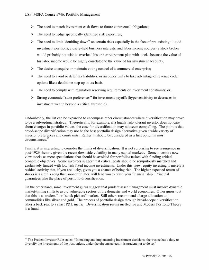
USF: MSFA Course #746: Portfolio Management
© Patrick Collins 107
The need to match investment cash flows to future contractual obligations;
The need to hedge specifically identified risk exposures;
The need to limit “doubling-down” on certain risks especially in the face of pre-existing illiquid
investment positions, closely-held business interests, and labor income sources (a stock broker
would probably not wish to overload his or her retirement plan with stocks because the value of
his labor income would be highly correlated to the value of his investment account);
The desire to acquire or maintain voting control of a commercial enterprise;
The need to avoid or defer tax liabilities, or an opportunity to take advantage of revenue code
options like a deathtime step up in tax basis;
The need to comply with regulatory reserving requirements or investment constraints; or,
Strong economic “state preferences” for investment payoffs (hypersensitivity to decreases in
investment wealth beyond a critical threshold).
Undoubtedly, the list can be expanded to encompass other circumstances where diversification may prove to be a sub-optimal strategy. Theoretically, for example, if a highly risk-tolerant investor does not care about changes in portfolio values, the case for diversification may not seem compelling. The point is that broad-scope diversification may not be the best portfolio design alternative given a wide variety of investor preferences and constraints. Rather, it should be considered as a first option in most circumstances.82 Finally, it is interesting to consider the limits of diversification. It is not surprising to see resurgence in post-1929 rhetoric given the recent downside volatility in many capital markets. Some investors now view stocks as mere speculations that should be avoided for portfolios tasked with funding critical economic objectives. Some investors suggest that critical goals should be scrupulously matched and exclusively funded with low-risk fixed income investments. Under this view, equity investing is merely a residual activity that, if you are lucky, gives you a chance of being rich. The higher expected return of stocks is a siren’s song that, sooner or later, will lead you to crash your financial ship. Principal guarantees take the place of portfolio diversification. On the other hand, some investment gurus suggest that prudent asset management must involve dynamic market-timing shifts to avoid vulnerable sectors of the domestic and world economies. Other gurus tout that this is a “traders’” or “stock pickers” market. Still others recommend a large allocation to commodities like silver and gold. The process of portfolio design through broad-scope diversification takes a back seat to a strict P&L metric. Diversification seems ineffective and Modern Portfolio Theory is a fraud.
82 The Prudent Investor Rule states: “In making and implementing investment decisions, the trustee has a duty to diversify the investments of the trust unless, under the circumstances, it is prudent not to do so.”

USF: MSFA Course #746: Portfolio Management
© Patrick Collins 108
CORRELATION AND ASSET ALLOCATION
The previous sections demonstrate how an efficient combination of investments with differing statistical characteristics enhances a portfolio’s risk/reward tradeoffs. This statistical-based method of portfolio construction stands in contrast to a technique that bundles investments sharing common statistical characteristics—safety of principal, forecasted capital appreciation, high current dividend or interest income, etc. —into a portfolio. In brief, the example illustrates how a combination of three securities generates a portfolio that achieves the expected return at a level of risk lower than any individual security. The pedagogical message of the admittedly stylized example is that the most favorable combination of securities includes an investment that, when viewed in isolation, promises comparatively low returns and high risk. The “best” portfolio includes the most “lousy” investment. A comparable example generally appears in most introductory investment textbooks in order to illustrate how combinations of assets with differing risk/return patterns offer an opportunity to create portfolios well suited to investor goals. More advanced investment texts use similar examples to introduce technical expositions on the mathematics of diversification.
IS DIVERSIFICATION AN EFFECTIVE STRATEGY FOR CONTROLLING PORTFOLIO RISK?
A key concept for understanding the principles of efficient (“scientific”) portfolio diversification is the correlation statistic. At the outset, it may be important to clarify why we are inviting you on a soporific journey by reading about a statistical concept. The central question that we wish to address is whether the recent bear market forces trustees to reassess the risk/reward benefits of portfolio diversification. In other words, is diversification an effective strategy for controlling portfolio risk; or, should it be relegated to the scrap heap? Understanding the concept of correlation is a prerequisite to understanding the limits of diversification. There is one more benefit to slogging through this material—once trustees grasp the limits of diversification, they are in a better position to formulate a coherent asset management strategy that fits the trust’s risk/return preferences.83 Without such an understanding, the trustee is condemned to be like the investor who jumps from investment to investment because he is enthralled by every new story spun out by a product salesperson. Or, at the limit, the trustee traps himself in an undiversified portfolio like the employee who loads up his or her retirement plan with company stock (e.g., Enron).
THE GEOMETRY OF CORRELATION
The essay previously defined correlation as “a measure of the linear association between two investments. If the return of investment A tends to be higher than its long-term average at the same time that the return of investment B tends to be higher than its long-term average, then the two investments are positively correlated. If the return of one investment tends to be lower than its long-term average while that of the other investment tends to be higher, then the two investments are negatively correlated. Finally, if the returns of each investment exhibit no linear association, the returns are not correlated. Uncorrelated returns have a correlation value of 0; returns that are perfectly correlated have a correlation value of +1;
83 Or, as expressed in §90 of the Restatement Third: “The trustee has a duty to the beneficiaries to invest and manage the funds of the trust as a prudent investor would, in light of the purposes, terms, distribution requirements, and other circumstances of the trust. (a) This standard requires the exercise of reasonable care, skill, and caution, and is to be applied to investments not in isolation but in the context of the trust portfolio and as a part of an overall investment strategy, which should incorporate risk and return objectives reasonably suitable to the trust.”

USF: MSFA Course #746: Portfolio Management
© Patrick Collins 109
and returns that are perfectly negatively correlated have a correlation value of -1. The correlation statistic can assume any value within the ±1 interval.” Geometrically, we can think of correlation as the interaction of return vectors. Working in a simplified two-dimensional coordinate plane [a “bivariate return distribution”], each return vector is a line through the origin if we set the initial period t – 1 return to zero. In two-dimensional subspace, if two returns are perfectly positively correlated they must point in the same direction; if perfectly negatively correlated they must point in opposite directions. Here are pictures of return vectors (arrows) in two-space for various values of the correlation statistic:
It is apparent that correlation depends on the angle formed by the two return vectors. More formally, for return vectors of equal volatility, correlation is associated with the cosine of the angle formed by the corresponding vectors. In linear algebra terms, for vectors X and Y, cosine equals the inner product of the two vectors [X·Y] divided by the product of the norm of vector X and the norm of vector Y, where norm is a measure of distance according to the Pythagorean Theorem: distance = [(X)2 + (Y)2]1/2. Our explanation stresses the fact that correlation is a measure of a linear dependence relationship only. Two results flow from this observation:
1. Some linear relationships result in spurious correlations. A well-known example is the correlation between ability in mathematics and children’s shoe-size. This correlation is spurious because older children are typically better in math than younger children; and, older children tend to have larger feet. Buying your youngster an ill-fitting pair of large shoes will not increase his or her scores on an arithmetic test! Courses in advanced statistics often discuss difficulties encountered when estimating correlations between data series that cannot pass tests for stationarity (infinite variance series). This is important in finance because random walk price evolutions are, by definition, non-stationary.
2. Two data series can have a zero value for the correlation statistic and, yet, exhibit a strong dependence structure because of a non-linear relationship. If, for example, X is distributed symmetrically around the origin and Y equals X2, then their correlation equals zero despite their perfect dependence: the X return vector equals (-2, -1, 0, 1, 2) and the Y return vector equals (4, 1, 0, 1, 4). The correlation between X and Y = 0 despite their non-linear dependence relationship.
X Y
Correlation = +1.0
X Y
Correlation = -1.0
X
X
Y
Correlation = 0.0 Correlation = +0.7Cosine(0.7) 45 degrees
YX

USF: MSFA Course #746: Portfolio Management
© Patrick Collins 110
Each of these observations has important consequences for portfolio design and management that we will discuss later in the article. We advance this somewhat technical explanation because many investors think that positive correlation means that two assets tend to increase in value at the same time, while negative correlation means that two assets tend to exhibit offsetting returns. This incorrect view can be expressed graphically as follows:
If this, in fact, were the case, combining assets with perfect negative correlation would take the portfolio nowhere fast—any gains made by investment X (blue) would be exactly offset by investment Y (brown). Combining the two investments into an equally-weighted portfolio guarantees no growth whatsoever! This incorrect view of correlation causes some commentators to observe that focused portfolios seeking high period-by-period performance are superior to portfolios formed by combining assets with low or negative correlation. This argument, although it sounds compelling, is specious. Consider an alternative, correct, view of negative correlation as expressed in the following chart:
- 1 0
- 8
- 6
- 4
- 2
0
2
4
6
8
1 0
1 2 3 4 5 6 7 8 9 1 0
- 1 0
- 8
- 6
- 4
- 2
0
2
4
6
8
1 0
1 2 3 4 5 6 7 8 9 1 0

USF: MSFA Course #746: Portfolio Management
© Patrick Collins 111
This graph also shows negative correlation (when asset X is above its mean return of 3%, asset Y is below its mean return of 3%, and visa-versa). However, there is a positive long-term rate of growth as evidenced by the upwardly sloping arrow. For example, X and Y are negatively correlated in period‘t’ if asset X earns 4% and asset Y earns 2%. Both assets increase in value but exhibit perfect negative correlation for the period because the returns fall on the opposite side of their respective means (averages).
CORRELATION AND RISK CONTROL
During the early period of Modern Portfolio Theory from the 1960s through the 1980s, knowledge of asset correlations was considered valuable in so far as it provided a guide to designing portfolios at an appropriate level of risk. The promise of Modern Portfolio Theory [MPT] is centered in its belief that the correlation structure of securities provides the key to controlling risk without sacrificing return. Portfolios built on MPT principles differ in approach from methods that accept low returns in exchange for principal guarantees. By forming portfolios of assets exhibiting differing pair-wise correlation values, overall risk is measured and controlled from the “portfolio context” rather than by aggregating low earning, stable-value assets. Let’s work through some examples to illustrate how MPT uses correlation as a “risk-control” input for portfolios.
Correlation = +1
2%
4%
6%
8%
10%
12%
14%
0% 2% 4% 6% 8% 10% 12% 14% 16% 18% 20% 22% 24% 26% 28%
Risk (Standard Deviation)
Return
A
B
Risk/Return Bound;Correlation = +/- 1
2%
4%
6%
8%
10%
12%
14%
0% 2% 4% 6% 8% 10% 12% 14% 16% 18% 20% 22% 24% 26% 28%
Risk (Standard Deviation)
Return
A
B
Risk/Return "Region"
Correlation = -1
2%
4%
6%
8%
10%
12%
14%
0% 2% 4% 6% 8% 10% 12% 14% 16% 18% 20% 22% 24% 26% 28%
Risk (Standard Deviation)
Return
A
B
-1 ≤ Correlation Value ≤ +1
2%
4%
6%
8%
10%
12%
14%
0% 2% 4% 6% 8% 10% 12% 14% 16% 18% 20% 22% 24% 26% 28%
Risk (Standard Deviation)
Return
A
B
-.5 +.4+.8

USF: MSFA Course #746: Portfolio Management
© Patrick Collins 112
Each of the above charts depicts the consequences of forming a portfolio from two assets: asset A has an expected return of 6% with a volatility of 8% as measured by its annualized standard deviation; asset B has an expected return of 12% with a volatility of 20%. If we choose to form a portfolio consisting of 100% asset A, all of the portfolio weight will fall on the point labeled ‘A.’ If we begin to blend A with investment B, the economic consequences differ depending on the value of the correlation statistic. The upper left chart indicates that as we move from a 100% investment in A to a 100% investment in B, the investment results trace out a straight line because the correlation value is a perfect +1. However, if the correlation value is at the opposite extreme—i.e., negative 1—then the upper right chart indicates that blending the two investments will result in the risk of A tending to offset the risk of B. Risk reduction continues until we arrive at a minimum risk portfolio. As the portfolio moves away from the minimum risk “blend,” the portfolio tracks either A or B more closely. The bottom left chart depicts the region of feasible investment combinations over the complete range of correlation values—i.e., ±1. The upper and lower correlation bounds carve out a risk/return region into which any two investments with known returns and standard deviations must fall. The riskiest spot in the region is located at the point where the portfolio consists of 100% B and 0% A. This point has an expected return of 12% with a standard deviation of 20%. The least risky spot in the region is located at the point where A and B combine for 0% risk—the minimum risk blend. This point has an expected return of slightly less than 8% with a standard deviation of zero. (You can tell that this is a highly stylized example because today’s risk-free rate is only about 1%--investors would love to earn a risk-free 8%!). The bottom right chart indicates that a combination of asset weightings and correlation values between ±1 determine the portfolio’s location within the feasible region’s risk/return space. Given a positive weighting of any asset, the portfolio is likely to be improved by combining the asset with an investment in a second asset with a low correlation value. The bottom right chart illustrates the risk/return profiles when asset correlations are -0.5, +0.4, and +0.8. The higher the value, the closer the portfolio tracks to the straight line (correlation = +1.0) at the edge of the region. Mixtures of assets with different pair-wise correlations create an aggregate portfolio with a more favorable risk/reward tradeoff. In general, a portfolio benefits more by adding assets with lower correlation values than with higher values, all else equal. Knowledge of correlation enables investments to be evaluated in a portfolio context rather than in isolation because it provides a clue to how investments interact over time. This observation gives rise to a classic problem in Modern Portfolio Theory—what is the optimal combination of assets given an investor’s return preferences and risk constraints. Harry Markowitz shared the 1990 Nobel Prize in Economics, in large part, because he provided a solution to this problem. THE PERIODIC TABLE OF INVESTMENT RETURNS REVISITED
You may recall the “periodic table” of returns presented in a previous section. We expand our view of this table by summarizing the asset class returns (i.e., the vectors of historically realized returns) into a more compact table of correlations (average pair-wise values of the correlation statistic):84
84 Table exhibits correlation values for the twenty-year period ending 2008.

USF: MSFA Course #746: Portfolio Management
© Patrick Collins 113
The classic definition of the portfolio design process entails the optimal combination of investments based, in part, on the correlation values like those exhibited in the above table. If certain simplifying assumptions are allowed, it can be demonstrated that there is a unique combination of assets that generates the highest expected returns for a given risk; and, the lowest level of expected risk for a given return. Financial economists term this unique combination “the optimal portfolio.” Furthermore, investing in any portfolio other than the set of optimal portfolios along the risk/return spectrum results in an unnecessary destruction of wealth in the sense that a non-optimal portfolio has expected returns insufficient to compensate the investor for risk. Correlation values seem to be the key to creating prudent investment portfolios.
RECENT RESEARCH: CAUSE FOR REASSESSMENT?
During the period that roughly spans the late 1980s through the present, probably no other area of academic research in finance has proved more fruitful than the study of how asset prices “behave.” Finance professors investigating the properties of the time series of returns from financial assets became skilled econometricians; and, with the aid of increased computer power, they developed a rich set of theories on the topic of dynamic asset pricing. Central to this research is a re-examination of the nature of correlation. Recent advances in econometrics--the application of statistical techniques to finance problems--have led, in some cases, to substantial modifications of the classic principles of Modern Portfolio Theory. The scope of the literature on financial econometrics is vast, and we provide only a brief discussion of some basic points. The classic definition of correlation relies, in part, on the central limit theorem. According to this point of view, there is a long-term average expected return which represents the central tendency for the growth of wealth under specific asset allocations. In any period, realized returns may be either above or below this central tendency; but, such deviations represent only temporary diversions from the true—but unobservable—central mean (called “the first moment”). Likewise, depending on the method of measurement, by the central limit theorem, there is a constant long-term parameter value for volatility (called “the second moment”). Risk-averse investors have a positive preference for a high first moment (average return) and a negative preference for a high second moment (volatility)—they like return and dislike risk. Although this economic world view allows for period-by-period variations in realized risks and returns, such variations are merely temporary perturbations from fixed long-term constant parameter
# Years
U.S. Large Company
Stock
U.S. Small Company
Stock
U.S. Micro Cap Stock
Securitized Real Estate
Foreign Large
Company Stock
Foreign Small
Company Stock
Emerging Markets Stock
U.S. 1-Year T-Bill
U.S. Intermediate
Bonds
World Government
Bonds
U.S. Large Company Stock
20 1.00 0.82 0.65 0.47 0.73 0.55 0.45 0.40 0.20 0.05
U.S. Small Company Stock 20 0.82 1.00 0.95 0.69 0.72 0.61 0.63 0.05 0.09 -0.04
U.S. Micro Cap Stock 20 0.65 0.95 1.00 0.72 0.61 0.55 0.55 -0.15 0.07 0.00
Securitized Real Estate 20 0.47 0.69 0.72 1.00 0.48 0.46 0.38 -0.04 0.07 -0.08
Foreign Large Company Stock
20 0.73 0.72 0.61 0.48 1.00 0.92 0.74 -0.05 -0.20 0.04
Foreign Small Company Stock
20 0.55 0.61 0.55 0.46 0.92 1.00 0.80 -0.13 -0.27 0.02
Emerging Markets Stock
20 0.45 0.63 0.55 0.38 0.74 0.80 1.00 -0.01 -0.08 -0.07
U.S. 1-Year T-Bill 20 0.40 0.05 -0.15 -0.04 -0.05 -0.13 -0.01 1.00 0.40 -0.17
U.S. Intermediate Bonds
20 0.20 0.09 0.07 0.07 -0.20 -0.27 -0.08 0.40 1.00 0.53
World Government Bonds
20 0.05 -0.04 0.00 -0.08 0.04 0.02 -0.07 -0.17 0.53 1.00

USF: MSFA Course #746: Portfolio Management
© Patrick Collins 114
values. Ultimately, this is a static, equilibrium-oriented system rather than a dynamic economic world view. Volatility differs from period-to-period; but, its long-term value is a constant—i.e., not time varying. Correlation—as the “byproduct” of asset returns and volatility—is also deemed, by the central limit theorem, to converge to an average or theoretical steady-state value. Econometricians call this constant value ‘unconditional correlation.’ Under the central limit theorem, the larger the sample (i.e., the longer the history of returns), the more confident the investor can be in the “true” (i.e., unconditional) value of asset correlations. Beginning in the late 1980s more powerful computers allowed financial economists to model asset returns such that volatility became volatile (time varying volatility) and correlations became dynamic (conditional correlation v. unconditional correlation). By the mid 1990s certain large institutional investment houses (e.g., J. P. Morgan) and consulting firms (e.g., BARRA) developed more sophisticated “risk metrics” capable of producing advanced computer-driven asset return models. Recent econometric research has, to some extent, turned some elements of classic Modern Portfolio Theory on their head—in 2005, for example, Markowitz published an essay arguing that the market portfolio is not efficient and that there is probably no linear relationship between an asset’s Beta and its expected returns.85 Current asset pricing theory now views return distribution parameters such as mean and volatility not as converging towards a theoretical steady-state constant value, but, rather, as dynamic values that must be adjusted both within differing regimes and across differing regimes. There may not be a true overall unconditional average like the central limit theorem suggests; rather, volatility and correlation values are conditional on the particular market regime—e.g., “bull” or “bear” market. Consider, for example the following graph of rolling three-year correlation between large capitalization U.S. stocks (the S&P 500) and large capitalization foreign stocks (the EAFE index) over the period 1976 through 2008.
85 Markowitz, Harry M., “Market Efficiency” A Theoretical Distinction and So What?” Financial Analysts Journal (September/October, 2005), pp.17-30.

USF: MSFA Course #746: Portfolio Management
© Patrick Collins 115
A correlation table fixes the value of the correlation statistic at 0.56 which is the average for the period. However, the actual three-year rolling correlation values range from a low of approximately 0.1 to a high of 0.92. Building a portfolio on the assumption that the average is a reliable parameter estimate seems not to be a particularly good idea. The above graph suggests two important facts about correlation:
1. It is an average taken over many years; and, like all averages, may not be representative of actual year-by-year values.
2. It is dynamic. Rather than forcing the correlation value to “fit” the entire period by assuming that it converges to a constant value, it may be more appropriate to split the time period into two or more regimes—e.g., a bull market regime and a bear market regime. If the correlation values shift dramatically from regime to regime, then building a portfolio based on an overall average may yield suboptimal results.
The second of the two facts leads some econometricians to argue that the most useful statistic is conditional correlation rather than absolute or unconditional correlation. Estimating a value for conditional correlation involves asking the following question: if the economy is currently in regime X, what is the likely linear association between one or more assets in this regime. This question is, of course, different from calculating the correlation values over all regimes within the sample period. Asset pricing models using conditional correlation values seem to produce models that better replicate the real world behavior of investment returns.
Conditional correlation calculations highlight not only the dynamic nature of correlation; but, also reveal a fact that is critical for risk control purposes. In severe down markets, volatility tends to increase (a higher standard deviation signifies that investment returns are more uncertain) and, most importantly,
Rolling 36 Month Period CorrelationsS&P 500 vs. Foreign Large Company Stocks (EAFE)
92.47%
0.00
0.10
0.20
0.30
0.40
0.50
0.60
0.70
0.80
0.90
1.00
1/1/1976 1/1/1979 1/1/1982 1/1/1985 1/1/1988 1/1/1991 1/1/1994 1/1/1997 1/1/2000 1/1/2003 1/1/2006 1/1/2009
Average = 0.56

USF: MSFA Course #746: Portfolio Management
© Patrick Collins 116
correlation values tend to increase. This observation has profound consequences for portfolio management. In a nutshell, during bear markets when downside volatility increases, increases in asset correlations make it less likely that the portfolio can emerge unscathed. If correlation is the key to efficient diversification, then increasing correlation values erode the benefits of diversification when it is most needed.
DIVERSIFICATION MELTDOWNS AND NEW POINTS OF VIEW
During the last several years, a flood of research has appeared on the topic of “diversification meltdowns” during periods of severe downside returns. Here is a brief recap of two important topics: First, correlation is only one measure of the possible dependence structures of financial return time series. It is a good dependence measure if the return series are multivariate normal (bell-curves) but a potentially misleading measure for non-normal time series. Unfortunately most publically traded assets (individual stocks and bonds as well as baskets of securities such as stock and bond index funds) flunk statistical tests for normality. Although they may flunk for a variety of reasons, the bad news is that financial returns are often leptokurtic. This means that they are “fat-tailed” and exhibit a propensity to manifest extreme results (both positive and negative) at a probability far greater than that found in normal distributions. This is not good news for risk-averse investors. Extreme downside volatility increases pair-wise correlation values so that many asset combinations appear to be headed into a death spiral simultaneously. This can be very scary.86 Second, financial return series exhibit a variety of extremely interesting non-linear associations. Cutting edge research is moving beyond correlation metrics into analysis of asset co-integration and portfolio copula structures. This research contains both good and bad news for investors. Let’s spend a moment on co-integration. The question to be entertained is this—if an asset price series is a random walk, where random walk is defined as “unpredictable” (readers of the famous book A Random Walk Down Wall Street by the economist Burton Malkiel87 know that under certain Modern Portfolio Theory models financial asset price changes follow a random walk88), can two random-walk asset price time series exhibit joint predictability? [Take a breath at this point because the intellectual waters get deep very fast]. According to classical statistics, a financial time series is “stationary” if the series has a constant mean, a constant variance, and a constant autocovariance--the correlation structure of its own current value and values in previous time periods—i.e., “lagged values.” A random walk price series is not stationary but, fortunately for investors, can be transformed easily into a stationary series by using a logarithmic transform of periodic returns [ln(asset price period 1 - asset price period 2) ÷ ln(asset price period 1)]. 86 Recent exploration of topics on “the butterfly effect”—a plunge in Los Angeles real estate values impacts orders for a factory in Dongguan, China—and on the “crowded trading effect”—liquidity demands like hedge fund margin calls require a widespread sale of collateral asset positions like TIPS that are traditionally uncorrelated with the margined account assets—indicate the limits of viewing correlation as a simple linear association tending towards a constant parameter value. 87 Malkiel, Burton G., A Random Walk Down Wall Street, W.W. Norton & Company, Inc. (New York, New York), 2003. 88 Technically, a random walk is usually modeled as a zero-mean martingale process. However, the time series of investment returns often exhibits characteristics comparable to a sub-martingale process with a drift component (expected return) and a diffusion component (standard deviation). A zero-mean random walk exhibits long periods of time in positive return territory and long periods of time is negative territory. Thus, it differs from a white noise process wherein returns rapidly oscillate between positive and negative values. A threshold requirement for demonstrating care, skill and caution appears to require the trustee to have some awareness of the nature and risks of the return generating process to which he is exposing trust wealth.

USF: MSFA Course #746: Portfolio Management
© Patrick Collins 117
This means that financial asset prices can wander a long way from their average values (the Dow Jones Index price level at the end of 1930 was 164, and wandered to 12,463 at the end of 2006) and may only rarely cross the moving average. Asset prices follow a random walk, and therefore, are unpredictable. If this sounds a lot like the Efficient Market Hypothesis, it should—because both points of view give expression to the same underlying mathematical concepts. Financial asset return series, however, are stationary and, therefore, are more tractable to computer modeling. A model of future returns can be applied to asset prices at a point in time (an “initial value condition”) to model the evolution of the price series. In classical statistics, by definition, two random walk price series have zero correlation. You don’t have a clue as to how series B will behave even if you know exactly what series A will do (as a matter of fact, you also don’t have a clue about series A’s future behavior but this is a different problem). Each series is random, exhibits no trend, and the pair-wise correlation must be zero. No association, no predictability—right? Wrong. Here is an example of a co-integrating relationship. Consider a dog that is wandering about a field. Its movements seem completely random—moving from spot to spot with no discernible purpose. Consider an inebriated man that is also wandering about the field. His movements seem completely random—moving from place to place with no discernible purpose. Although there should be no “dependency structures” to be found in uncorrelated vectors of motion; nevertheless, if the man is the owner of the dog, it is unlikely that the dog will wander too far away from its master. Uncorrelated random walks can exhibit a formal dependency structure—i.e., they can be co-integrated. Robert Engle and Clive Granger shared the 2003 Nobel Prize in economics, in part, for their studies of financial asset price behaviors including common trends such as co-integrating relationships and autocorrelation values. Copulas provide very good news for investors because they offer new ways of looking at how the “marginal distributions” of individual assets (the return distributions of assets considered in isolation) relate to the “joint distributions” of portfolio components as they dynamically interact. Although the mathematical complexities of copula structures make it unlikely that they will appear any time soon at your local financial planner’s office, nevertheless, as the underlying mathematics become better understood, the “dangers” of using only an unconditional correlation metric in portfolio design and asset management should also become better understood. We illustrate how copula functions can capture risk characteristics of financial asset returns that correlations miss. Correlation is a valid risk-control metric only when distributions manifest a symmetric, linear dependence structure. Copulas, by contrast, capture asymmetric tail dependence. Here are two pictures of a normal mixture copula density. A normal mixture assumes that each of the financial return series is normal; but, that means and variances are conditional on the regime (bull or bear market). Graph one illustrates results assuming a -0.1 correlation value; graph two illustrates results assuming a +0.7 correlation value. Note that the base of the graphs is a unit square representing the possible range of correlation relationships.

USF: MSFA Course #746: Portfolio Management
© Patrick Collins 118
Graph One:
Graph Two:
0.50.751
1.251.51.752
2.252.52.753
3.253.53.754
4.25
0.50.751
1.25
1.5
1.75
2
2.25
2.5
2.75

USF: MSFA Course #746: Portfolio Management
© Patrick Collins 119
The two graphs look very different from the bell-curves that usually represent normal distributions. Bell curves have most of the probability mass in the center, and the tails are relatively skinny.89 Extreme events are considered to be unlikely. Copula structures also exhibit skinny tails (located in the four corners), but they do a much better job capturing higher corner values. This reflects the relative importance of tightening correlations (i.e., greater dependence) in extreme market conditions.
NEW APPROACHES AND OLD REMEDIES
As the dust settles on the global bear market, investors ponder whether they should reexamine their macro allocation (ratio of stocks to bonds). MPT suggests that stock risk is manageable in the portfolio context because securitized real estate, emerging markets stocks, and blue-chip U.S. stocks manifest differing pair-wise correlation values. Further research, however, suggests that this statement should be modified—the asset classes manifest differing pair-wise correlation values on average. In extreme volatility regimes, however, the correlation values often differ significantly from their historical averages; and, in down-market regimes, the pair-wise correlation values may move towards +1. For investors who elected to assume certain bond risks by holding junk (high-yield) bonds or mortgage-backed debt instruments, the recent convergence of the correlation structure towards unity was particularly devastating. So the question now is do we go back to a static blueprint for investment decision making or do we rethink how best to manage wealth in a more dynamic context? During the depths of the global recession some trust companies advocated a stay-the-course posture because, in their view, stocks were “on sale.” It was a good time to re-commit to equities because they were likely to go up in value as the business cycle moved out of the recession. Other trust companies sought to re-assess a trust’s tolerance for risk as a first step in selecting a new long-term macro allocation. The strategy often involved increasing the relative portfolio weight to short-term fixed income instruments that may be government guaranteed with respect to payments of interest and principal. The astute reader may recognize that the financial advice profession has, to a great extent, landed clients back into the old fear/greed decision making structure that has been discredited for decades! Decisions are driven by a P&L metric (“today’s the day to make money” / “don’t lose any more money”) that, at the end of the day, is not helpful. For all of the advances in financial economics, it seems as if some trustees are returning to the days of using investment nostrums from yesteryear to cure current portfolio ills. Is there a credible solution path? The answer to this most important question forms the subject matter of the next section.
APPROACHES TO ASSET ALLOCATION, REVIEW OF RECENT ACADEMIC OPINION, AND
A CASE STUDY
Restatement Third Trusts and its statutory “derivative,” the Uniform Prudent Investor Act, require an understanding of principles of financial economics on the part of trustees and their legal counsel. This requirement flows, in part, from the duty to invest funds with appropriate care, skill and caution. Indeed, care, skill and caution have become defining characteristics of prudence in modern trust administration. Good faith and absence of speculation may no longer be adequate defenses against breach of fiduciary
89 The Copula graphs also have most probability mass in the center because the graph is a three-dimensional square and the surface area covered by values close to the median is greater than the surface area covered by the “skinny” tails.

USF: MSFA Course #746: Portfolio Management
© Patrick Collins 120
duty allegations involving investment decisions--especially when a trustee advertises special skills and expertise. Before reviewing recent approaches to the asset allocation paradigm, it is worth noting that there is a growing chorus of opinion suggesting that MPT is “wrong” and that following the “prescriptions” of MPT is dangerous and may, in fact, increase litigation risk.90 If the author may be allowed a brief editorial aside, this seems very much a straw man argument. It is akin to quoting medical science textbooks published in the 1960s and concluding that medical science should be ignored and modern doctors should not be trusted because subsequent research found that certain statements in their med-school textbooks were incorrect.
STRATEGIC ASSET ALLOCATION IN PORTFOLIO MANAGEMENT: SELECTING AND CONTROLLING
EXPOSURES TO SYSTEMATIC RISK
The function of strategic asset allocation in portfolio management is to integrate the investor’s return objectives, risk tolerance, investment preferences and constraints with long-term capital market expectations in order to enhance investor utility. The concept of utility is key to the development of credible and defensible trust investment strategies. Utility is a numerical measure of ‘happiness’ or ‘satisfaction’ with the portfolio. Specifically, a utility function is a mathematical expression of a preference relationship—e.g., an investor prefers x to y, y to z, and, therefore x to z. Investors generally have a positive preference for return and a negative preference for risk—i.e., risk aversion. The greater a portfolio’s utility value, the more the investor prefers it to portfolios with alternative allocations. Thus, we restate our initial proposition […the primary purpose of asset allocation is to set the investor’s long-term exposure to systematic risks] as follows: the primary purpose of strategic asset allocation is to increase utility by establishing appropriate exposures (weightings) to asset classes. One benefit of efficient asset allocation is risk reduction. Variance is a common measure of portfolio risk.91 The greater the value of the variance statistic, the greater is the uncertainty of the final outcome. A portfolio’s variance [σ2—‘sigma’ squared is the Greek symbol for variance] is commonly expressed as:
tww2
Where, is the variance/covariance matrix (correlation structure); and ‘w’ is the vector of asset weights (asset allocation).92 Strategic asset allocation is a function of (1) long-term capital market expectations (efficient market equilibrium expected returns) or (2) long-term capital market forecasts (active management’s forecasted views). An efficient portfolio is one which produces the highest expected return for a given value of portfolio variance; or, the lowest level of variance for a given expected return.
90 In a legal context, see, for example, Sterk, Stewart E., “Rethinking Trust Law Reform: How Prudent is Modern Prudent Investor Doctrine?” Cornell Law Review (Vol.95, 2010). 91 The square root of variance is standard deviation. The greater the value of the standard deviation statistic, the more uncertain the outcome—the realized return of an investment may differ greatly from the expected or forecasted return. Therefore, a lower standard deviation is generally preferred to a higher standard deviation, all else equal.. 92 wt is the transpose vector of ‘w.’ Variance is a squared or second order term the calculation of which requires the squaring of the asset allocation weighting vector.

USF: MSFA Course #746: Portfolio Management
© Patrick Collins 121
Controlling the magnitude of the variance term through efficient asset class weighting is an important objective of asset allocation.93 When risk is defined as the variance of the portfolio’s returns, the total risk of portfolio ‘j’ can be decomposed into Systematic Variance and Unsystematic Variance. In the single factor CAPM market model, total risk can be expressed as:
2222ejmjj
Where Beta [B] is the slope of the characteristic line of a regression analysis [independent variable is the
market / dependent variable is portfolio ‘j’]; where 2m
is the variance of the broad stock market and
where 2ej
equals the variance of the error term—the portion of return not attributable to the aggregate stock and/or bond market.
Total Portfolio Risk = Market Related Risk + Investment Specific Risk
But, in the portfolio context, the variance of the error term goes toward zero as the number of assets grows large.94 Expected portfolio risk is a function of the number of securities within the portfolio and the correlation structure of the securities. In a multifactor model, the sources of risk may include both beta (market risk) as well as other systematic risk factors. Thus, beta can encompass a variety of risks—not just an investment’s sensitivity to its comparative benchmark.95 The beta of a stock can be (1) the CAPM beta—a measure of how sensitive the stock is to up and down market movements; (2) an accounting beta—a measure of how sensitive the stock is to changes in general corporate earnings; (3) a liquidity beta—a measure of how sensitive the stock is to aggregate demand to buy or sell; (4) a small cap beta—a measure of sensitivity to small company risks; (5) a value beta or “recession” risk sensitivity; (6) an inflation beta, etc. It is important to define what you mean by the term “Beta” [Beta = one or more systematic risks] lest there be unwarranted confusion. Sometimes one hears a statement like “Beta is not a useful measure of an investment’s risk.” Without sufficient context, such a statement is almost devoid of meaning. Thus, on a preliminary basis, we can define asset allocation as the process by which a trustee (1) selects systematic risk exposures appropriate for the purposes, terms, distribution requirements and other circumstances of the trust, (2) selects appropriate assets to provide the desired risk exposure(s), and (3) weights the assets within the portfolio to conform with the trust’s return preferences and risk constraints. The realities of modern asset allocation often take the trustee far from the world of the single-index CAPM model in which, for a diversified portfolio, the relevant measure of long-term systematic risk is a portfolio’s market Beta.96 Two basic tenets of financial theory are:
93 Note that in this expression the variance/covariance matrix (correlation structure) is static. Risk is controlled by varying the weight of the asset classes. 94 The Capital Asset Pricing Model assumes that error terms are independent. By definition, independence assumes zero correlation. 95 The beta of U.S. stock investments is often derived by reference to the S&P 500 index; foreign stock investment betas are often derived by using the EAFE [Europe, Australian & Far East] index as a comparative benchmark, and so forth. 96 From time-to-time some commentators suggest that portfolio allocation should be ‘risk factor allocation’ rather than ‘asset class allocation.’ That is to say, the trustee should identify the risk exposures which are appropriate, and derive a weighted exposure to each risk factor such that the total portfolio risk is acceptable. One difficulty to such an approach is that it may be difficult to accurately forecast the expected return from each risk factor exposure. Risk allocation, however, remains a promising field for future research.

USF: MSFA Course #746: Portfolio Management
© Patrick Collins 122
1. in the long run, the returns earned on a diversified portfolio are reliably related to the portfolio’s exposures to systematic risk; and,
2. only systematic risks should be rewarded because all other risks can be diversified away.
Much of the Third Restatement’s Prudent Investor Rule discusses the implications of these two propositions. The traditional view assumes that strategic asset allocation specifies the investor’s desired exposures to systematic risk(s). From the 1980’s onwards, there has been a fruitful research effort to develop a more sophisticated understanding of risk and to develop more insightful ways to measure, profile, and manage it. An understanding of econometric research requires a somewhat high level of mathematical and analytical skill. However, many of the insights of recent econometric research inform the tasks of portfolio design and asset management. Therefore, it is critical for a trustee representing that his organization possesses investment acumen to document that the trust’s allocation is the product of a prudent—credible and defensible—decision making process.
THE IMPORTANCE OF ASSET ALLOCATION FOR PORTFOLIO PERFORMANCE
Several academic studies discuss the importance of asset allocation to the long-term risk/return characteristics of the investment portfolio. The importance of the asset allocation decision on long-term investment results is a subject of some controversy. Conventional wisdom, based on a 1986 study, suggests that the asset allocation decision is the primary determinant of return for portfolios with long-term planning horizons.97 That is to say, asset allocation explains much of the variation in returns over time:
Determinants of Portfolio Performance
Other Factors
Market Timing
Asset Allocation
Security Selection
0 20 40 60 80 100
From a short-term perspective, these findings are counterintuitive because stock selection and transaction timing have a significant impact on short-term returns. But focusing on the short term can be detrimental for investors with longer planning horizons. Indeed, the study found that market-timing activities actually subtracted returns from portfolios over planning horizons longer than ten years. However, the study does not explain the reasons why individual portfolio returns differ from each other—that is to say, it does not
97 Brinson, Gary P., Hood, Randolph L., and Beebower, Gilbert L., “Determinants of Portfolio Performance,” The Financial Analysts Journal July/August, (1986), pp. 39-44. See also, Brinson, Gary P., Singer, Brian D., and Beebower, Gilbert L, “Determinants of Portfolio Performance II: An Update,” Financial Analysts Journal, Vol. 47, #3 (1991), pp. 40-48.

USF: MSFA Course #746: Portfolio Management
© Patrick Collins 123
examine the cross-sectional variation of returns [why fund A’s returns differ from fund B’s v. what explains fund A’s return variance over time]. However, another recent study suggests that, even over long planning horizons, security selection should dominate asset allocation decisions with respect to its affect on portfolio performance. The study outlined five factors that could explain investment returns: (1) asset allocation, (2) country allocation, (3) global industry sector allocation, (4) country-specific industry sector allocation, and (5) security selection.98 The authors isolated each factor and simulated 10,000 portfolios (60% stock/40% fixed income asset allocation) using data from 1987 through 2001. Portfolios based on the security selection factor had the greatest range of returns; portfolios based on the asset allocation factor had the smallest dispersion of returns. Therefore, at least theoretically, the authors conclude that security selection has the greatest potential for influencing long-term investment returns.99 Other studies come to different conclusions. For example, a 2000 study argues that the importance of asset allocation depends on the investment question under consideration.100 Specifically, the investor might be interested in knowing:
1. What percentage of a portfolio’s ups and downs (variability in return) is explained, over time, by its asset allocation choices? [EXPLAIN VARIANCE] or,
2. How much of the performance difference between two distinct portfolios can be explained by differences in their asset allocation? [EXPLAIN RETURN DIFFERENTIALS] or,
3. How much of a specific portfolio’s actual returns can, over time, be explained by its asset allocation? [EXPLAIN TIME SERIES OF RETURNS]
These are very different questions and require separate methods of analysis. The authors decompose monthly returns of balanced mutual funds over a ten-year period into a ‘policy’ return (the return attributable to the fund’s asset allocation), and an ‘active’ return (the remaining return). The study confirms that approximately 90% of the variability in the returns of the average fund can be explained by its asset allocation decisions [EXPLAIN VARIANCE]. When funds are compared to each other, however, the conclusion differs. If two funds select the same asset allocation and each invests in the same cross-section of passively managed indexes, 100% of each fund’s variation of returns across time would be attributable to asset allocation policy. Likewise, if two funds had the same asset allocation policy but each invested in a separate set of securities, asset allocation would explain 0% of the return differences over time. In fact, however, the mutual funds under evaluation differed with respect to their asset allocations and their security selection, market timing, fees and other factors. The study concludes that, on average, asset allocation decisions account for about 40% of the variation of returns across funds [EXPLAIN RETURN DIFFERENTIALS]. Bottom Line is that asset allocation explains 90%+ of the variation in returns over time; or explains 40%+ of cross-sectional
98 Kritzman, Mark & Page, Sebastien, “The hierarchy of Investment Choice: A Normative Interpretation.” The Journal of Portfolio Management, Spring 2003. 99 The titles of several recent research studies suggest that asset allocation is unimportant to financial success. For example, Munnell, Alicia H., Orlova, Natalia Sergeyevna & Webb, Anthony, “How Important is Asset Allocation To Financial Security in Retirement,” Center for Retirement Research at Boston College, (April, 2012) concludes that their data “suggests a minor role for asset allocation in creating a secure retirement.” However, this is primarily due to the fact that most retirees have such a small nest egg that a decision like working longer will dominate any asset weighting decision. The best allocation can do little good if the portfolio is not worth much. 100 Ibbotson, Roger, & Kaplan, Paul, “Does Asset Allocation Policy Explain 40, 90, or 100 Percent of Performance?” Financial Analysts Journal, Vol. 56 No. 1, pp. 26-33.

USF: MSFA Course #746: Portfolio Management
© Patrick Collins 124
variation in the returns of different funds. Either way, asset allocation is an important determinant of long-term performance. Finally, the authors test for the percentage of individual fund returns that, over time, can be explained by asset allocation [EXPLAIN TIME SERIES OF RETURNS]. This is the ratio of policy return divided by total actual return. A hypothetical fund with a consistent asset allocation policy implemented by a purely passively investment strategy will, by definition have a ratio equal to one—total return is policy return. Funds exhibiting ratios greater than one will have subtracted value through active management decisions (actual total returns in the denominator fail to equal the policy returns in the numerator); funds exhibiting ratios less than one will have added value through active management decisions regarding security selection and market timing. The distribution of ratio values is interesting. The median result (50th percentile) was 1.00—on average, actively managed mutual funds neither added nor subtracted value during the period under evaluation. The best actively managed funds exhibit ratios of 0.82; however, the worst performing funds exhibit ratios of 1.32. These results suggest that the risk of selecting active management for a trust portfolio is not symmetric because the downside risk has a magnitude greater than upside reward.
APPROACHES TO ASSET ALLOCATION: MEAN–VARIANCE, RESAMPLED EFFICIENT FRONTIER,
BLACK–LITTERMAN, MONTE CARLO SIMULATION, ALM, EXPERIENCE BASED, AND ADAPTIVE
ASSET ALLOCATION
A comprehensive discussion of the many approaches to asset allocation would require a book-length manuscript. The following is a short-list of some widely discussed allocation methods. Mean Variance Optimization: This approach, first pioneered by Harry Markowitz,101 has a strong basis in capital market theory as it employs capital market expectations along with investor risk aversion, preferences and constraints to design an optimal asset allocation. However, it is very sensitive to small changes to the inputs to the Markowitz calculation algorithm—i.e., the model is prone to estimation error. This is especially true if the input relies on the average of historical returns—the estimator is ‘unbiased’ but ‘inefficient.’ Usually, estimation error in the expected return input has greater impact than estimation error in the variance/covariance matrix values. Mean Variance Optimization software programs are sometimes derisively referred to as “mistake maximizers.” Resampled Efficient Frontier: This approach recognizes that critical inputs to Mean/Variance optimization are known only with a high degree of uncertainty.102 Small changes in forecasted returns can produce large changes in optimal asset allocations. The Resampled approach simulates a large number of possible return evolutions and optimizes across each of the possible efficient frontiers within the range of outcomes. The portfolios are ranked, and the resampled frontier is the average of the asset class weightings at each rank (with the percentile of results ordered from lowest to highest return). The strength of this solution is that it creates more diversified portfolios that do not strictly rely on the single path of either historical results or forecasted point-estimate parameter values. The approach, however,
101 Markowitz, Harry, Portfolio Selection: Efficient Diversification of Investments, New Haven, Connecticut (Yale University Press), 1959. 102 Economists use the term ‘mean blur’ to characterize uncertainty of expected returns.

USF: MSFA Course #746: Portfolio Management
© Patrick Collins 125
lacks a strong basis in capital market theory and does not take into account estimated equilibrium returns given the relative weighting of asset classes in today’s world market portfolio.103 Black-Litterman: There are two versions of the Black-Litterman [B/L] approach:104 The unconstrained approach (no sign restrictions on asset class weights) takes the weights of the asset classes in a global benchmark (e.g., MSCI World) as a neutral starting point. The asset weights are adjusted to reflect the investor’s views on expected returns according to a Bayesian procedure that also takes the strength of the investor’s confidence about the views into account. The reverse engineering approach derives implicit equilibrium expected returns given the relative asset weightings within the global benchmark. It then combines these “estimated” returns with the investor’s unique views, adjusting for confidence levels, to derive the B/L view-adjusted return forecasts. These forecasts are, in turn, used as the inputs to a mean/variance optimization. The B/L approach has a strong basis in capital market theory, takes into account equilibrium market conditions, and tends to result in well-diversified portfolios. The linear algebra needed to build effective algorithms is, however, complex; and, for many practitioners, B/L approaches are merely a black box. The output of the model is a function of implied equilibrium expected returns adjusted for (1) the investor’s forecasted returns; and (2) the confidence the investor has in the accuracy of the forecasts. In essence, the B/L approach blends the market portfolio with the investor’s opinions to derive a revised probability distribution of future returns. This revised distribution is then optimized to obtain an efficient frontier. Simulation [Monte Carlo]: Simulation is fast becoming the preferred method for asset allocation decision making. This approach calculates a range of possible future outcomes derived from a risk model that incorporates the statistical characteristics of multiple asset class return series. Future evolutions of wealth are generated under random scenarios for investment returns, inflation, and other relevant values (e.g., longevity for trust income beneficiaries). Simulation is critical to create numerical solutions in the presence of path dependency (e.g., cash flows, fees, trading costs, etc.). Simulation is often used to specify the probability of a future shortfall in assets relative to trust objectives. However, great care must be taken in the development of the risk model lest the output suffers from misspecification [model risk]. Unfortunately, many commercial software programs assume that investment distributions are ‘normal’ or, in a multi-period context, ‘lognormal.’105 Asset/Liability: The Asset/Liability management [ALM] approach combines both assets and liabilities in the analysis of the optimal portfolio. Often the objective is to obtain growth in the surplus (assets minus liabilities) subject to certain risk constraints. ALM can incorporate each of the above listed asset allocation approaches. It’s strength lies in its ability to model liability exposures through short positions
103 Michaud, Richard, “The Markowitz Optimization Enigma: Is Optimized Optimal?” Financial Analysts Journal, Vol. 45 No. 1, (1989) pp. 31-42. See also, Michaud, Richard, Efficient Asset Management. Boston, Mass. (Harvard Business School Press), 1998. 104 Black, Fischer, & Litterman, Robert, “Asset Allocation: Combining Investor Views with Market Equilibrium,” Journal of Fixed Income, Vol. 1, No. 2 (1991), pp. 7-18. See also, Idzorek, Thomas, “A Step-By-Step Guide to the Black-Litterman Model,” Working paper (Stanford University), 2002. Litterman, Bob, “Global Equilibrium Expected Return,” and “Beyond Equilibrium, the Black-Litterman Approach,” Chapters Six and Seven in Modern Investment Management, (John Wiley & Sons, 2003), pp. 55 – 88. 105 That is to say, the shape of the distribution of expected returns is symmetrical—like a bell curve—with approximately 99% of outcomes falling within three standard deviations above or below the average. It is rare to find a commercially available program that allows the user to construct a risk model in which correlations and volatility are time varying, inflation is stochastic, and longevity risk is something other than life expectancy. Furthermore, it has been pointed out that the more widely used programs often generate outputs with vastly different risk assessments and projected values. Milevsky, Moshe A., & Abaimova, Anna, “Will The True Monte Carlo Number Please Sand Up?” Working Paper, The IFID Centre (March 2006).

USF: MSFA Course #746: Portfolio Management
© Patrick Collins 126
in appropriate mimicking portfolios. However, it is subject to misspecification of the mimicking portfolio when changes in liability values are not market related.106 One of the more promising directions in the recent evolution of portfolio design and implementation is the incorporation of shortfall risk metrics--as quantified through simulation of credible risk models--to an ALM allocation approach. Advances in computer technology allow trustees to track not only long-term shortfall risk but also the likelihood of breaching within-horizon minimum value thresholds. This enables the trustee to monitor insolvency risk—the risk that the present value of trust assets is less than the present value of current beneficiary and remaindermen “claims.”107 Experienced Based: These approaches rely on financial planning “rules of thumb.” Here is an example: A prudent investment strategy is to own a portfolio with a proportional weighting to stock equal to 100 – the investor’s current age. One advantage, especially for unsophisticated beneficiaries, is that such rules are often easy to understand intuitively—i.e., little quantitative analysis skill required. However, it is often difficult to justify a rote application of these rules to trusts with differing preferences, positions, and constraints. Adaptive Asset Allocation: This approach, promulgated primarily by William Sharpe,108 points out that maintaining a static investment policy under all economic conditions does not maintain a constant exposure to systematic risk. Security price changes contain information regarding the consensus view about the distribution of future expected returns. For example, the value of the aggregate U.S. or world stock market changes constantly relative to the aggregate value of the aggregate U.S. or world bond market. When the ratio of aggregate stock market value increases relative to aggregate bond market, the consensus investor opinion reflects optimism regarding future stock returns. When the ratio decreases, the reverse is true. For a 60-40 stock-to-bond portfolio, maintaining a constant percentage weighting during a period when stock-bond dollar values are 50-50 means that the investor’s portfolio is more risky than the general market. An Adaptive Asset Allocation approach recommends changing the portfolio’s asset weighting over time to reflect changes in market values even if there has been no change in the investor’s risk/return preferences. This approach is not commonly used because of the difficulty in obtaining information regarding current dollar values of aggregate world market indexes. There are many variations on and combinations of the above approaches. As a consequence, no bright-line standard of practice for developing and implementing an asset allocation policy exists.109 This said, it is becoming less likely that an approach based primarily on selecting twenty to fifty stocks from the “recommended list” of an affiliated research department, monitoring investment holdings based on analyst buy/hold/sell recommendations, and controlling risk by limiting sector exposures or individual stock weights will remain a defensible approach to asset allocation. The trend appears to call for
106 For an extensive discussion on this approach to trust asset management see Collins, Patrick J., “When All Choices Are Bad….” ALI-ABA Course of Study Materials: Representing Estate and Trust Beneficiaries and Fiduciaries (San Francisco, 2012); and, “Managing Modest-Sized Family Trust portfolios: Issues in Income Adequacy and Portfolio Sustainability,” ALI-ABA Course of Study Materials: Representing Estate and Trust Beneficiaries and Fiduciaries (Chicago, 2011). 107 Claims might take the form of providing sufficient distributions under an ascertainable standard criterion, preserving principal value for the remaindermen, etc. For a discussion of portfolio optimization in the face of a defined liability structure see “Rethinking Asset Allocation” Vision Focus (State Street), June 2012. The State Street term for monitoring within-horizon portfolio value is “Full-Scale Optimization.” 108 Sharpe, William F., “Adaptive Asset Allocation Policies,” Financial Analysts Journal (May/June, 2012), pp. 45 – 59. 109 It is interesting to speculate on the consequences of the absence of a bright line standard of practice. Does this encourage trustees to concentrate on making their portfolios look like those offered by other trust departments? Is there a rush towards uniformity in asset allocation policy to the exclusion of thoughtful consideration of the terms, purposes, distribution requirements and other circumstances of each trust?

USF: MSFA Course #746: Portfolio Management
© Patrick Collins 127
utilization of a risk model110 in order to identify the portfolio’s risk exposures and to demonstrate portfolio feasibility in terms of (1) matching expected returns to the trust’s economic requirements, and (2) aligning the magnitude of potential risks with the trust’s risk constraints. IX. Taxes / Diversification / and Active Investment Management Conventional wisdom suggests that active investment management is best able to meet the needs of private taxable investors. However, the concept of tax Alpha added through active investment management has critical implications for portfolio design and implementation. The individual investor’s initial portfolio should be highly diversified because of its propensity, over time, to build up embedded gains as the market value of appreciating securities exceed their original cost. Indeed, there is an inherent tension between active investment management and the likelihood for increased recognition of tax liabilities caused by active management. Active management, by focusing on concentrated security selection may, if successful, create conditions that destroy both the need for and feasibility of continued portfolio management. This occurs when gains become so great over time that they become “locked into” the portfolio: “It also may well expose the portfolio to the risk that it ‘freezes’ at some point—when there is so much unrealized gain in all positions that no further trades, and thus management, can possibly make sense. Once frozen, the portfolio no longer can earn excess returns, and may in fact trail the market because of bets that are no longer attractive. Further, it is exposed to rising risk over time….” Taxable portfolios must be sufficiently diversified at the time of their inception so that the client remains comfortable holding them for the long term. The concept of “lockup” returns us to the active/passive investment debate. A default method of tax management is to invest in a capitalization-weighted index fund. Such an investment has three advantages: (1) it is broadly diversified and reflects the consensus ideas of all portfolio managers and investment decision makers; (2) the fund tends to move in lockstep with the index and, because it requires little rebalancing in order to stay in alignment, it tends to delay realization of capital gains; and (3) turnover within the index is usually low and, therefore, the tax cost of ongoing rebalancing also remains low. It may be preferable, according to the authors, to be passive with respect to investment management and active with respect to tax management. Concentrated portfolios are particularly subject to portfolio lockup. They are retained at inefficient risk or are diversified at a large tax cost: There is a dynamic conflict between lockup and diversification when managing portfolios in the presence of taxes. Active investment management is difficult because the dual goals of seeking a security selection alpha and a tax-managed alpha work against one another. When an active manager generates returns in excess of the market, the excess returns generate additional taxes. Thus, a key issue is the amount of excess return that the active manager must generate to equal the after-tax results of a passive strategy. Taxes and diversification (strategies for low basis stock) is the subject of the Jean L.P. Brunel article in the readings for this Section. Brunel creates a “life cycle” of concentrated equity ownership that consists of three stages:
110 Early examples of such a model are J.P. Morgan’s RiskMetrics and the BARRA portfolio risk analysis programs both of which are now owned by MSCI.

USF: MSFA Course #746: Portfolio Management
© Patrick Collins 128
1. Entrepreneurial—in which the founder of a business holds most of his wealth in the form of stock of a new “unseasoned” company. Despite the high degree of company-specific risk, the entrepreneur is not inclined to diversify for a variety of reasons including lack of a market, stock control issues, and upside price change potential.
2. Executive—The stage of ownership for stock in newly public companies. Unique risk is still very high but the company now has a wider market and benefits from increased liquidity. Founding shareholders may no longer exercise a high degree of control and may be more inclined to begin a process of diversification.
3. Investor—In this stage, the investor moves away from the single stock position to a more prudent balanced and diversified portfolio. If the investor wishes to eliminate all unsystematic risk, the new portfolio will employ a strategy of indexing to achieve maximum diversification.
Brunel lists several techniques that are commonly used to diversify a concentrated low-basis position. These include: Outright Sale Exchange Partnerships Completion Portfolios Hedging Strategies
In his opinion, the preferred diversification technique is hedging: “Hedging strategies have become the technique of choice for low-basis diversification….” The asset manager, however, must be particularly sensitive to the U.S. tax code regulations defining “constructive sales.” Knowledge of constructive sale regulations, which are both complex and, seemingly, ever changing, is not required in this course. You should be familiar, however, with the merits and disadvantages of the more popular hedging techniques:
1. Collars (especially, the concept of the “cashless collar”); 2. Hedge + monetization; and 3. Variable pre-paid forwards (a form of ‘deferred sale’).
X. Previous Exam Questions 1. An individual investor, several years away from retirement, establishes a personally owned,
discretionary investment account with a Bank’s Private Wealth Management division. The “know-your-client” forms signed by both the Bank and the investor, at the time of account opening, marked the checkbox “growth” next to the Investment Objective category; and marked the checkbox “above-average” next to the Risk Tolerance category. The Bank established a 100% stock portfolio invested in a cross-section of U.S. large-cap (“blue-chip”) and mid-cap growth stocks. The account does not have an Investment Policy Statement. Unfortunately, the portfolio lost 50% of its market value over a three-year period. The client has initiated legal action charging the Bank with a breach of fiduciary duty. The client contents that the Bank knew that the account represented the major portion of the “nest egg;” and that the Bank should have established a more appropriate investment allocation.
The Bank, however, has asked a judge for “summary judgment” ordering the case to be
dismissed without trial. The Bank notes that, although the account was discretionary, they

USF: MSFA Course #746: Portfolio Management
© Patrick Collins 129
communicated each investment transaction to the client (via trade confirmations, monthly
account statements and quarterly investment recaps). The Bank’s argument for dismissal is
based on the fact that the client “ratified” the investment actions by not voicing his
disapproval; or, that the client could veto the actions and order the trades to be reversed. The
client, therefore, exercised “control” over the account. Furthermore, the Bank argued that the
client was free to fire them if the client was uncomfortable with the investment process or
dissatisfied with the investment results. The fact that the client waited three years before
taking action suggests that the case is nothing more than “sour grapes.” The client contends
that he periodically voiced concern over mounting investment losses. However, the Bank’s
account representative assured him that, in the long run, equity outperforms other assets and
that the client should ‘stay the course.’
You are asked to provide insight from the perspective on an investment professional.
Discuss the merits and liabilities of the Bank’s theory of the case.
2. Assume that state insurance commissioners will not allow insurance carriers to issue policies that
offer a positive net present value expected return to policyholders. Offer two reasons, based on portfolio theory, why prudent asset allocation for a young individual investor starting a career may include purchase of a disability income policy. [Note: disability income policies replace a portion of an insured’s earned income if, due to sickness or accident, he or she is unable to work in their occupation.]
3. Two clients, each age 35, come to your office to seek advice regarding portfolio asset allocation.
Client one is a recently tenured college professor in the economics department; while client two is a recently hired MBA starting an executive position at a technology firm.
Identify the important objectives and constraints of a well-constructed written
investment policy;
Speculate on how investment policy for each client might differ given his or her respective career paths; and
Construct a hypothetical asset allocation for each client and justify your recommendations.

USF: MSFA Course #746: Portfolio Management
© Patrick Collins 130
4. A husband and wife, without children or other dependents, visit your office shortly after they retire. You are engaged to help them develop, write, and implement an Investment Policy Statement [IPS] for a retirement income portfolio.
What economic and personal risk factors may be most significant for this couple?
What information would you want to elicit from them in order to help you better understand the nature and magnitude of their retirement risks?
How might you quantify each risk factor?
How might the investment strategies and guidelines contained in the IPS address each risk?
5. Comment on the following investment opinion regarding ownership of a diversified portfolio of
stocks:
“Confining oneself to situations convincing enough to be entered on a relatively large scale is a great help to safety and profit. One must know far more about it [i.e., the stock] to enter the position in the first place….A large number of small [stock] holdings will be purchased with less care and ordinarily allowed to run into a variety of small losses without full realization of the eventual total sum lost. Thus over-diversification acts as a poor protection against lack of knowledge.”
Appendix I: Office of the Comptroller of Currency [OCC] guidelines for Bank Fiduciary Activities OPTIONAL READING—THIS MATERIAL WILL NOT BE TESTED Banks are increasingly providing services to private high-net-worth investors. The Director’s Book, published by the OCC, provides the following caution for banks attempting to expand their traditional fiduciary activities beyond employee benefit and private trust departments: “Many large banks have established a private banking department, offering a full array of investment management services, including fiduciary services, to high net worth individuals. As the fiduciary business continues to evolve, the wide variety of products and services, frequently offered in locations outside of the traditional trust department, presents a complex administrative challenge to bank boards. Regardless of the scope of the fiduciary activities, however, the board is responsible for monitoring its administration. The board must protect the bank’s fiduciary reputation, as well as the assets of the customer, by having effective policies and procedures, management information systems, and risk management practices. The board should confirm that individuals who administer fiduciary activities at the bank are knowledgeable, competent, and have high personal integrity….” The OCC lists several areas of concern: [NOTE: The following list outlines a prudent procedure for banks]

USF: MSFA Course #746: Portfolio Management
© Patrick Collins 131
“When considering fiduciary activities, the following practices or conditions should trigger additional board scrutiny: The opening of new accounts not in compliance with account acceptance guidelines.
To protect the bank’s reputation as a fiduciary, and thereby minimize reputation risk, the bank must know its customers. The board should establish, or delegate the establishment of, guidelines designed to make sure that only accounts that meet the board’s selection standards are accepted. An account acceptance process helps prevent the opening of new accounts with unclear objectives, accounts that management is not qualified to administer, accounts that may lead to conflicts of interest, and accounts that may expose the bank to future liabilities such as from environmental hazards….
The purchasing of securities not previously approved by the board or investment committee.
The board or investment committee normally establishes investment guidelines and approves investment lists to control the acceptable amount of risk. Any security purchase that falls outside of established guidelines should be carefully evaluated to determine its suitability for an account. Management should document its decision to purchase such an asset.
Higher than anticipated yields on investment portfolios, collective investment funds, or advertised mutual funds.
Investment managers who are rewarded solely on the performance of the portfolios they manage may have an incentive to accept more risk in order to increase returns. Even if the securities purchased are authorized for the account or fund, the manager may be taking undue risks….
The existence of accounts with unusually high cash balances or large or extended overdrafts.
A fiduciary is responsible for properly managing fiduciary assets. High cash balances in accounts may indicate that management is failing to meet its responsibility to make fiduciary assets productive. Similarly, large or extended overdrafts may indicate poor management of an account….
Failure to institute adequate internal controls for fiduciary activities. Indications that internal controls are weak include references to numerous or repeat exceptions to policies and procedures in internal reports, internal or external audits, or in examination reports…. Losses or settlements arising from actual or threatened litigation that are significant in either size or volume. Losses or settlements may indicate that fiduciary assets are not being administered properly. The board should require management to explain thoroughly any significant losses or litigation, and make an effort to identify the cause of the problem. The board should then determine that the underlying reason for the problem has been corrected. Numerous or increased amounts of customer complaints also may indicate administrative weaknesses. To mitigate reputation and litigations risks, the bank should ensure that all customer complaints are investigated and addressed by management to ensure that customers are being properly served. Any situations that give rise to a conflict of interest. To protect the bank’s reputation as a fiduciary, the board should direct management to implement policies and procedures to avoid conflicts of interest and even the appearance of conflicts….” Appendix II: After-Tax Asset Location OPTIONAL READING—THIS MATERIAL WILL NOT BE TESTED

USF: MSFA Course #746: Portfolio Management
© Patrick Collins 132
Appendix II is intended to provide students with a glimpse into current debate on the issue of whether it is best to own certain assets in a tax-favored retirement account or in a taxable account [The Asset Location Debate]. We begin with an article authored in 1996 by William Ghee and William Reichenstein of Baylor University.111 This important article develops the concept of ‘tax alpha.’ The authors define this term as “the additional after-tax rates of return attributable to tax structures.” The returns earned by stocks and bonds differ depending on whether they are held in tax-deferred accounts or in taxable accounts. A tax alpha is a characteristic of certain tax-favored accounts, and it is measured in terms of a benchmark defined as “the after-tax rate of return that the individual could earn by holding the bond or stock in the personal tax structure.” The authors argue that the Alpha generated by the tax structure of savings vehicles is more important than investment manager alphas in long-term wealth accumulation: “The investor with average stock-picking skills who saves in the pension tax structure will almost always retire with more wealth than the superior stock picker who saves in an account subject to the personal tax structure.” According to the authors’ calculations, “the ending after-tax wealth on stocks held in the pension is 60 percent larger after 20 years than if the same stocks were held in the benchmark personal tax structure.” Some financial advisors extend, not entirely appropriately, the authors’ findings into a rationale for loading tax-deferred retirement accounts with equity. However, pointing out that holding equity in a retirement account produces greater wealth than owning equity in a taxable personal account is not the same as demonstrating that equity ownership within a tax-deferred account is favored over bond ownership within a tax-deferred account; and, that loading equity-oriented investments into retirement plans will result in a higher utility of overall wealth. The article is thus an important source for the asset location debate over whether it is best to own stocks within or outside of a retirement account. Additionally, the authors note that annuities provide a third tax structure for investors—namely the ability to contribute after-tax dollars to a tax-deferred savings vehicle. However, annuities, in general, lack sufficient tax-alpha to overcome their high fees: “Insurance companies charge annual fees on deferred annuity contracts. Unfortunately, the typical annual fee of 1.25% usually exceeds the tax advantages of the deferred-annuity tax structure.” In 2000, John Shoven & Clemens Sialm reexamine the asset location debate.112 The authors point out that investments held in tax-deferred accounts are not, in general, perfect substitutes for investments in taxable accounts because investments in tax-deferred accounts have both a higher expected return and higher risk (as measured by standard deviation). The higher expected returns are a result of compounding in a tax-favored environment. However, the after-tax returns from equity held in a conventional savings account are less variable because realized capital gains increase the tax liability while realized losses decrease the tax liability: “This symmetric tax system dampens both gains and losses.” The authors agree with the proposition that the optimal asset location significantly enhances retirement resources; but argue that it is the combination of expected return, standard deviation and the tax rates facing the returns that dictates the preferred asset location. The optimal location decision rests primarily on “the proportion of returns that the equity fund distributes annually as dividends and capital gains (tax effect). Only funds with high annual (potentially taxable) distributions should be located in a TDA [tax deferred account].” In the authors’ model, equity will be held in the TDA if the annual distributions of the equity fund are above
111 Ghee, William & Reichenstein, William, “The After-Tax Returns from Different Savings Vehicles,” Financial Analysts Journal (July/August, 1996), pp. 62-72. 112 Shoven, John & Sialm, Clemens, “Asset Location in Tax-Deferred and Conventional Savings Accounts,” National Bureau of Economic Research Working Paper 7192 (April, 2000).

USF: MSFA Course #746: Portfolio Management
© Patrick Collins 133
17%. Furthermore, according to their model, the optimal asset location increased the benefits of the TDA by 6.7 percent. The paper also discusses the option to invest in municipal bonds. Historically, the implicit tax rate on munis (1 – rm/rb, where rm and rb denote the nominal returns of municipal and corporate bonds) has been lower than the marginal tax rate of high-income taxpayers. The authors contend that the implicit tax rate on municipal bonds has historically been in the neighborhood of 30%. Conventional financial planning wisdom states that high bracket individuals should own tax-exempt bonds if the marginal tax rate on their ordinary income is higher than the implicit tax rate on munis. However, according to the authors, the relevant comparison is the implicit tax rate on municipal bonds vs. the tax on stocks: “Individuals should put [taxable] bonds in the TDA and mostly stocks in the [conventional savings account] if the taxes on stocks are lower than the implied taxes on municipal bonds. This reduces the demand of investors for municipal bonds….” One key implication of this argument is that an investor’s demand to hold municipal bonds decreases with the availability of tax-efficient equity vehicles (e.g., index funds and Exchange Traded funds). A 2001 research monograph by James Poterba at MIT advances the proposition that it is important to separate an asset’s risk characteristics and its tax attributes.113 Differing tax attributes lead to the concept of “asset habitat.” The habitat issue complicates the portfolio optimization problem. Differences in post-tax payoffs will influence decisions on asset allocation (i.e., the shape and location of the post-tax efficient frontier). For long-term investors, estimations of future tax rates (government tax rate schedules, tax policy, as well as changes in future labor income) also complicate the portfolio choice problem. Tax law complications may be an important factor in explaining why lower wealth households often hold undiversified portfolios. For example, the accounting burdens and costs of owning just a single real estate partnership may overwhelm any diversification benefit from including the asset within a small investment portfolio. Studies suggest a link between tax rates and portfolio structure: the probability that a household owns tax-favored assets (low dividend stocks or tax-exempt bonds) is a positive function of the household’s marginal tax rate. The author argues that highly taxed bonds should be held in the tax-favored account: “This is a pure ‘tax arbitrage’ in the sense that the household’s after-tax return can be increased without changing its risk exposure.” However, households seem to own both equity and taxable fixed income investments in both taxable and tax-deferred accounts—this is an asset location puzzle. That is to say, “relatively few investors are choosing markedly different asset allocation patterns in their taxable and in their tax-deferred accounts.” Following the work of Poterba, Shoven and Sialm, most academic studies advocate owning equity in taxable accounts and taxable bonds in retirement accounts. Indeed, since 2002, a kind of disconnect has developed between academic prescriptive advice and the planning recommendations given by a large segment of financial advisors. One reason for the disconnect may be traced to the complexity of the topic. The scope of potential complexity is the topic of an address by Nancy Jacob to the New York Society of Security Analysts in 2002.114 Jacob points out that private client portfolios are complex because they often include (1) Fully taxable Sub-portfolios (Grantor trusts, personal portfolios); (2) Tax-Advantaged Sub-portfolios (401(k)s, IRAs, Variable Annuities, Charitable Remainder Trusts); and, (3) Tax-Exempt Sub-Portfolios (Life Insurance
113 Poterba, James M., “Taxation and Portfolio Structure: Issues and Implications,” National Bureau of Economic Research Working Paper 8223 (February, 2001). 114 Jacob, Nancy L., “Advanced Tax-Aware Asset Allocation and Location,” New York Society of Security Analysts conference (January, 2002).

USF: MSFA Course #746: Portfolio Management
© Patrick Collins 134
policies, Private Foundations). Additionally, tax exposures occur in two dimensions—income tax and estate tax: “The more estate tax exposure you have, the more taxes you’re going to ultimately pay and you have to think about having growth assets in those portfolios versus income-producing assets…” Restructuring existing portfolios is especially complex because of possible imbedded capital gains and other transaction costs. Tax aware asset allocation becomes a function of the portfolio’s starting point: “it is almost like a Markoff Chain. The starting point determines the ending point.” [A Markoff Chain is a period-by-period evolution of a system from its current state to a future state when the evolution is governed by (sometimes known) transition probabilities]. Simple rules of thumb like ‘put-all bonds-in-an-IRA’ are difficult to apply because of the complexity and relative sizes of the sub-portfolio accounts. Generally, however, “Where you have the highest tax rates, you want to have the most tax-efficient type of management, and passive generally is more tax-efficient than active management.” An excellent synthesis between the findings of academic research (characterized by mathematical modeling) and the practitioner community is found in Don Mulvihill’s 2003 essay entitled “Asset Allocation and Location.”115 Mulvihill states that the tax code allows investors to use various entities for purposes of income, gift and estate tax planning. Entities include qualified retirement plans, grantor trusts, private foundations, charitable trusts and so forth. Optimization techniques can be used to determine both the ideal asset allocation plus asset location. For example, a common function to optimize is “subject to funding my consumption needs, maximize the risk-adjusted real value of wealth that will be received, net of income and transfer taxes, by my intended heirs and charitable beneficiaries.” According to Mulvihill, as a general rule, the optimal solution usually entails (1) shifting of highly appreciating assets to estate tax –favored entities like a grantor trust; and, (2) shifting income tax-inefficient assets into qualified plans. Mulvihill echoes the academic advice for funding qualified plans but extends the rationale for locating bonds in the retirement account beyond a consideration of income taxes into the area of estate-taxes: “All return earned or accrued within the retirement account will be subject to ordinary income tax when it is withdrawn. Any balance left over when both parents have died will be subject to ordinary income tax. The remaining balance will then be subject to estate tax and will not have the benefit of the step-up in basis….it makes little sense to shift highly appreciating assets that generate long-term capital gains rather than ordinary income into the retirement account.” While Mulvihill extends the rationale for owning taxable bonds within the retirement account by considering the complex interactions of income, gift and estate tax law, Ashraf Zaman from Purdue University published a monograph in 2004 that increases the number of assets beyond a single stock and a single bond usually considered in academic model building. The increase in assets introduces new dimensions of correlation and portfolio rebalancing as factors in the asset allocation and asset location decisions.116 These considerations modify the general rule advocating that preference be given to bonds over equity within the tax-deferred account. The author begins the essay by acknowledging the tradeoff between utilization of the tax timing option to defer gain recognition and the benefits of diversification: “In a taxable account, investors have incentives to realize capital losses yet defer capital gains…. Over time, following this strategy will lead to a poorly diversified portfolio.” Most economic models consider the asset allocation / asset location decision in terms of a two-asset portfolio. However, when multiple risky assets are considered, their correlation structure is often a key determinant of investor choice. By placing some equities in the TDRA [tax deferred retirement account], investors can “freely trade these assets to maintain a diversified portfolio without incurring the tax consequences.” The author develops a model that incorporates two risky assets
115 Mulvihill, Don, “Asset Allocation and Location,” Modern Investment Management edited by Bob Litterman (2003), pp. 565-578. 116 Zaman, Ashraf, “Asset Location and Allocation with Multiple Risky Assets,” Working Paper, Krannert Graduate School of Management, Purdue University (March, 2004).

USF: MSFA Course #746: Portfolio Management
© Patrick Collins 135
under various correlation parameter values and under various borrowing and short sale constraints. Other key factors include the investor’s bequest motives and the “retirement wealth ratio” (fraction of total wealth held in the retirement account). The author develops an equation denoting the change in net cash flow assuming that an investor shifts from stock to bonds in the tax deferred account and from bonds to stock in the taxable account. Given that the tax on ordinary income is higher than the tax on capital gains, and that interest rate on bonds is higher that the dividend rate on stocks, the investor is “strictly better off holding the bond in the tax deferred account and holding stock i in the taxable account.” Having made this observation, the author notes two “schools” of academic advice: (1) the yield-driven investor choice rule that says that tax deferred accounts should be funded with the assets with the highest yields (yield is defined as the percentage of total return distributed to the investor); and (2) the tax-rate investor choice rule that says “the preferred asset location is determined primarily by the tax rates facing the asset returns, and assets with the high tax rates should be allocated in the tax-deferred account.” Zaman’s model, however, predicts various mixes of bonds and equities in both tax-deferred and taxable accounts. Investors with most retirement funds in tax-deferred accounts will hold high amounts of equity in these accounts in order to stay close to their desired asset allocation targets. However, “for low retirement wealth ratio, almost 100% of the retirement wealth is allocated to bonds.” For investors with lower retirement wealth ratios (most assets held in the taxable account), the demand to hold equity in taxable accounts increases. This is especially the case for investors with high bequest motives. Indeed, older investors have an increasing demand to hold equity to capture the step-up in basis tax options and because they must finance consumption for heirs over long periods. As the value of the correlation coefficient decreases, the diversification benefits of equities increases (at perfect negative correlation, all of the retirement account is funded with equities—“the diversification value simply outweighs the tax timing option value”). When correlation values are close to zero or positive, however, no equities are held in the TDRA if the investor has no borrowing constraints (i.e. can utilize margin loans on taxable brokerage accounts). Likewise, investors with lower bequest motives tend to hold almost zero equity in the TDRA. In June of 2004, three finance professors co-authored an important article in The Journal of Finance on the topics of asset location and asset allocation.117 The authors explore the interrelationships between the asset allocation decision (“deciding how much of each asset to own”) and the asset location decision (“deciding which assets to hold in the taxable and tax-deferred accounts”). The study is, in part, motivated by their desire to test the wisdom of conventional advice: “Financial advisors commonly recommend that investors hold a mix of stocks and bonds in both their taxable and tax-deferred accounts, with some financial advisors recommending that investors tilt their tax-deferred accounts toward equity.” Conventional advice seems to inform the asset location decisions of many investors. For example, the authors report that 48.3% of investors who own taxable bonds in taxable accounts also own equity in tax-deferred accounts, and 53.1% of the owners of tax-exempt bonds also own equity in tax-deferred accounts. The research study employs “arbitrage arguments” to test the optimal location of asset holdings. The arbitrage approach involves a risk-free shift in the location of assets (i.e. moving a dollar of taxable bond holdings either into or out of a tax-deferred account in favor of an “equivalent” after-tax dollar of equity holdings). The authors develop a series of equations designed to identify “…the asset location policy that produces the highest expected utility of after-tax wealth.” The equations require sufficient complexity to reflect the fact that (1) the value of a dollar located in a tax-deferred account (the government will tax withdrawals as ordinary income) is not equal to the value of a dollar located in a taxable account; (2) investors face differential tax rates on investment returns; and (3) investors face differing borrowing and
117 Dammon, Robert M., Spatt, Chester S. & Zhang, Harold H., “Optimal Asset Location and Allocation with Taxable and Tax-Deferred Investing,” The Journal of Finance (June, 2004), pp. 999-1037.

USF: MSFA Course #746: Portfolio Management
© Patrick Collins 136
lending constraints on their taxable accounts. In order to reduce the dimensionality of the problem to manageable proportions, the authors employ the arbitrage approach under the assumptions that (1) the investor has a choice of investing in one of two assets (a riskless bond—either taxable or municipal) and an equity ‘portfolio;’ and, (2) the investor must realize all capital gains and losses each year. This last condition is deliberately restrictive in order to test financial planning advice under the most unfavorable circumstances for holding equity within a taxable account. In practice, equity provides investors with valuable options with respect to lifetime tax liability timing or step-up in basis elections at death. The equations demonstrate that the change in after-tax wealth generated by a shifting a dollar is independent of the stochastic growth rate of equity (bond interest and stock dividends are modeled as constants) and, therefore, a change in wealth “represents a risk-free after-tax payoff that can be generated by shifting the location of asset holdings.” However, there is no guarantee that a positive change in after-tax wealth in either the tax-deferred or taxable account will, in fact, produce positive utility with respect to total wealth. The source of the uncertainty lies in the fact that the tax structure affects changes in the taxable and tax-deferred accounts differently. To preserve the results of the arbitrage argument, the authors successfully undertake the burden of verifying, under reasonable assumptions regarding investment yields and tax rates, that the investor is “strictly better off holding taxable bonds in the tax-deferred account.” The study extends the analysis to recent changes in U.S. tax law wherein equity dividends and capital gains are taxed at the same rate, while interest income is taxed at a higher rate: ‘this implies that it is not optimal to hold equity in the tax-deferred account, regardless of the magnitude of the dividend yield on equity.” The authors reverse the common financial advice and advance the proposition that “it is tax efficient to hold equity (or equity mutual funds) in the taxable account and taxable bonds in the tax-deferred account if taxable bonds have higher yields.” The study revisits the argument advanced by Shoven and Sialm that suggests the opportunity to hold municipal bonds in the taxable account may change the optimal asset location decision. They verify the viability of such a strategy by substituting a shift from equity to a municipal bond rather than to a taxable bond within their arbitrage argument framework; and, under certain conditions, they verify that it is optimal for an investor to hold equity in the tax-deferred account and tax-exempt bonds in the taxable account. However, under reasonable assumptions regarding returns, distributions and tax rates, the mutual fund would have to be highly tax-inefficient to justify owning it in a tax-deferred account. The authors make two points: (1) the mutual fund would have to distribute approximately 75% of its capital gains each and every year; and (2) the presence of tax-efficient index funds implies that, in general, the superior strategy is to hold tax-efficient equity in the taxable account. The authors conduct a ‘certainty-equivalency’ analysis and determine that an actively managed mutual fund must generate a “pre-tax abnormal return (before transaction costs and fees) of 165 basis points or more…before it is beneficial to hold the actively managed equity mutual fund in the tax-deferred account.” They conclude: “…the opportunity to invest in tax-exempt bonds does not alter the optimal asset location policy provided equity can be held in a relatively tax-efficient form.” The study presents a simulation model assuming that the investor does not leverage the taxable account (i.e., does not avail himself of margin loans). The model suggests that equity appears in the tax-deferred account only under a limited set of circumstances; and then, only in limited amounts. For example, if an investor has little taxable wealth, the demand to hold equity in the tax-deferred account in order to achieve an overall optimal asset allocation would increase. However, the tax-inefficiency of equity held in a tax-deferred account makes investors reluctant to substitute equity for taxable bonds unless the tax-deferred account is so large relative to total investable wealth that the investor must take reasonable steps to avoid becoming too underweighted in equity. Parenthetically, the model also indicates that older investors with strong bequest motives have an increasing demand to hold equity because of the forgiveness of capital gains at death and because they are faced with high mortality rates (i.e., the step-up

USF: MSFA Course #746: Portfolio Management
© Patrick Collins 137
in basis option becomes increasingly valuable). Again, this observation contrasts with the more common financial advice to decrease equity exposure during retirement. The study continues by calculating the utility costs to investors electing to follow the conventional advice suggesting that they should first allocate equity to the retirement account before holding it in the taxable account. The penalty to investor utility is measured in terms of “computing the amount of additional wealth…that is needed to equate the investor’s total expected utility under the suboptimal location policy to that under the optimal location policy.” The penalty is greatest for younger investors who will incur a higher utility cost because they maintain the suboptimal asset location policy over a longer planning horizon. The estimated utility costs are in the neighborhood of 15%. The concluding section explores the utility of precautionary savings in an investor’s financial planning strategy. In order for holding bonds in the taxable account to be attractive, there must be a positive probability of a liquidity shock sufficiently severe to drive the investor’s standard of living below an acceptable minimum threshold. Additionally, the amount of funds in the taxable account must be insufficient to cover the magnitude of the liquidity shock. The risk of holding equity in the taxable account rests on the fact that: “if equity values decline significantly, it may be necessary …to incur a penalty to liquidate a portion of the tax-deferred accounts to finance consumption.” The simulation model suggests, however, that with the exception of a few years just prior to retirement, most liquidity shocks would not justify deviating from the tax-optimal allocation and location policies. These cases, however, involve simulations wherein the value of the taxable account relative to total wealth is small; and, therefore, would not apply to most investors, in the authors’ opinion. Investors living this ‘close-to-the-bone’ appear to adapt to a positive probability of liquidity shocks less through asset location strategies and more through a tendency to reduce their contributions to retirement accounts. The CFA Institute published a comprehensive treatise on the topic of tax efficient wealth accumulation in 2005.118 The book defines the relationships between asset allocation (“…how an investor allocates his or her investment portfolio among different asset classes.”) and asset location (“…how assets are distributed among taxable accounts and TDAs”) [Tax Deferred Accounts]. The author builds a step-by-step framework to analyze investment decision making under a variety of taxable regimes. He begins with a detailed analysis of the “simple” choice between a ‘front-end-loaded’ tax favored account like a traditional IRA, and a ‘back-end-loaded’ account like a Roth IRA. Front-end-loaded accounts include 401(k) and Keogh Plans, and refer to the tax deductibility of the initial contribution. Back-end-loaded accounts include Roth 401(k) and 529 College Savings plans, and refer to the lack of deductibility for the initial contribution, and the withdrawal of funds on a tax-free basis. Both types of accounts offer investors the opportunity to accumulate earnings on a tax-deferred basis. If there is no change in the applicable tax rate (a pivotal assumption) the present value of the future tax liability on withdrawals from a traditional IRA will exactly equal the present value of the extra taxes paid by virtue of the non-deductibility of contributions to a Roth IRA. The nominal taxes on the entire corpus of the traditional IRA are, of course, greater; but “properly discounting these future taxes at the opportunity cost of capital exactly offsets their nominal growth.” The investor considering which tax-advantaged vehicle to use, however, soon discovers a myriad of complications. Analysis is difficult because of the arcane terminology associated with the dual lexicons of tax law and financial economics, and because of the economic consequences of a tax system that embodies differential rates and recognition rules. That is to say, a dollar in one type of tax environment is not worth a dollar in another. Horan’s monograph, however, seeks to work through the dense thicket of tax and investment variables by creating algebraic models under certain simplifying assumptions (e.g., constant investment returns and
118 Horan, Stephen, Tax-Advantaged Savings Accounts and Tax-Efficient Wealth Accumulation (The Research Foundation of CFA Institute), 2005.

USF: MSFA Course #746: Portfolio Management
© Patrick Collins 138
constant pre and post retirement tax rates). The reader is then free to plug in values representative of his or her personal situation in order to arrive at a ‘first order’ understanding of the financial consequences of investment elections. Although it is intuitively easy to see that a traditional IRA [IRA] is valuable if the contribution tax rates are high, while the Roth IRA is valuable if the withdrawal tax rates are high, a formal analysis requires the investor to decide whether the comparison will be on a pre- or a post-tax basis. The author uses the contribution limits for the 2004 tax year ($3,000) as the point of departure. Suppose an investor in the 25% tax bracket wishes to make a contribution of $3,000. The IRA account receives a total after-tax investment of $3,000 while the Roth IRA account receives a total after-tax investment of $2,250 because the contribution was not deductible and, therefore, required the investor to pay ($3,000 x .25) $750 in taxes. Alternately, one can compare the two accounts by noting that a $3,000 contribution to an IRA generates a $750 tax deduction. Thus the investor can contribute the ‘extra’ $750 to a taxable investment account. A Roth IRA, on the other hand, requires a total investment of $4,000 in order to reach the $3,000 contribution limit of the IRA ($4,000 x .25 = $1,000) because the investor must pay taxes on the entire contribution. Thus, a $4,000 Roth IRA contribution equals a $3,000 traditional IRA contribution, a $750 contribution to a taxable investment, and a $250 payment in taxes to the federal treasury. The total after-tax IRA investment equals $3,750 compared to the total after-tax Roth IRA investment of $3,000. A moment’s reflection reveals that the pre-tax contribution allowable under the tax code for an IRA is greater than the contribution limit for that IRA (with the excess earmarked for a taxable account). As stated, this gets very complicated very fast. The point of the preliminary numbers crunching, however, is to illustrate that one can use either pre-tax or post-tax comparisons with equal validity provided that the tax consequences are fully accounted for and provided that any applicable tax savings are appropriately invested. Horan’s analysis, therefore, solves a major academic debate over the merits of comparing the accounts on a pre- or post-tax basis. Unfortunately, however, it introduces another complicated dimension to the analysis—the decision making involved in investing the supplemental taxable account. For investors wishing to maximize their pre-tax contributions, the attractiveness of the traditional IRA will, in large measure, stand or fall based on the taxability of the taxable side account. This, in turn, requires yet a more complicated round of algebra to model the future value interest factors attributable to current contributions to both tax-favored and taxable accounts, where taxable accounts are subject to differential tax rates and where future taxes must reflect adjustments to basis caused by payment of taxes in the present. At this point, the “dimensionality” of the problem (i.e., the number of relevant variables) increases substantially. Variables can also include the planning horizon, the assumed investment return, the assumed pre and post retirement tax rates and the assumed investment characteristics of the taxable side account (ordinary income, capital gains, gain recognition rates, and so forth). The author provides illustrative tables for investors in various tax brackets under differing planning horizons and investment returns. A change in any one of these variables may alter the relative attractiveness of the investment options significantly. Additionally, a critical variable is the amount of change, if any, from pre- to post-retirement tax bracket. Horan cites evidence that, on average, post-retirement income is about 64 percent of pre-retirement income. For a married couple filing jointly with an adjusted gross income of $180,000, such a decrease would drop them two tax brackets in retirement to a marginal rate of 25 percent. Indeed, across many planning horizons and investment return rates, “…the optimal choice between a traditional IRA and a Roth IRA depends largely on the tax rate prevailing when the funds are withdrawn.” Horan offers several observations: If the investor drops two tax brackets during retirement, the traditional IRA is nonetheless
optimal because the benefit of the low withdrawal tax rate outweighs the disadvantage of the taxable investment associated with the traditional IRA strategy. When the same investor drops

USF: MSFA Course #746: Portfolio Management
© Patrick Collins 139
only one tax bracket, the traditional IRA is optimal only for short time horizons or for investments with low rates of return” [e.g., short and intermediate term fixed income investments].
Establishing both types of accounts may provide investors with a useful tax option: “…an investor with both types of accounts may choose the account from which withdrawals are made prior to the mandatory withdrawal age of 70 1/2 years.” This is “akin to a real option in a capital budgeting context.”
The tax characteristics of the supplemental taxable account may profoundly influence the investor’s choice between traditional and Roth accounts. The lower the tax-drag in the taxable account, the greater the attractiveness of the traditional IRA account at the maximum contribution level. Thus investors with low-cost and low-turnover passively managed investment portfolios will tend to favor traditional IRAs.
Investors subject to the Alternative Minimum Tax may wish to lower their adjusted gross income by making contributions to a traditional IRAs in order to avoid or mitigate the phase out of exemptions that occurs as AGI increases.
Investors benefiting from employer matches to front-end-loaded accounts will find these types of 401(k) options almost always more valuable that back-end-loaded options lacking a contribution match provision.
Converting a traditional IRA to a Roth IRA is attractive only if the tax liability triggered by the conversion is paid from funds in a highly taxed account. Otherwise the investor’s tax rate at withdrawal must increase by about 11% (i.e. a 25% marginal tax bracket investor must find himself in the (1.11x..25 = 27.75) 28% tax bracket after retirement to compensate for the payment of taxes and early withdrawal penalties.
Horan’s study continues with interesting discussions of a variety of topics including comparisons between non-deductible IRAs and taxable investments, early withdrawal penalties and breakeven horizons, and so forth. Of special interest is a lengthy discussion of valuation of assets held within tax-sheltered accounts. Recognizing that retirees buy goods and services with after-tax dollars rather than with pre-tax dollars, Horan develops a formula for determining the taxable equivalent of a pre-tax dollar held in a tax favored account: “…that is, the amount of taxable assets that would produce the same after-tax cash flow as a withdrawal from the tax-sheltered account at some future date.” The important message is that the determination of the value of a pre-tax dollar is strictly relative to the investment strategies and returns applied over the applicable planning horizon within the taxable account alternatives. In other words, depending on the tax efficiency and expected returns in the taxable account (not to mention the investor’s tax bracket), a pre-tax dollar might be worth either more or less than an equivalent dollar within the taxable account. The later chapters of the research monograph address the issue of asset location—should stocks be owned in taxable accounts or in tax shelters? The asset location decision, “…involves a series of trade-offs. On the one hand, the higher expected return associated with equity investments increases the value of deferring taxes on their return (as opposed to bond returns)…suggesting stocks might be optimally located in tax-deferred accounts. On the other hand, the effective tax rate on equities is lower than on fixed-income instruments, suggesting stocks might be optimally located in taxable accounts.” Horan provides a nice summary of research on the asset location topic. For example, arguments in favor of owning stocks in tax-sheltered accounts include: Active investors may wish to hold stocks in tax-sheltered accounts if frequent trading generates
substantial amounts of short-term gains;

USF: MSFA Course #746: Portfolio Management
© Patrick Collins 140
Stocks may be the optimal holding for tax-sheltered accounts if the planning horizon, expected return, withdrawal pattern, and the applicable investor tax brackets result in an after-tax valuation of a dollar within the tax-sheltered account greater than $1.00;
The opportunity to purchase municipal bonds in a taxable account may tip the scale in favor of using tax-shelter dollars to purchase stocks.
Investors with strong precautionary savings motives may prefer to have highly liquid, low risk portfolios that can be used to finance consumption requirements in times of economic shocks. Stocks, given their greater volatility and the possible positive correlation between their returns and the investor’s labor income (i.e., during recessions, stock prices are likely to decline as job layoffs increase), are best placed in tax-sheltered accounts.
However, after applying the after-tax valuation method (i.e., determining the ratio of after-tax goods and services that can be purchased by the income stream from the taxable account and the after-tax goods and services that can be purchased by the income stream from the tax deferred account), Horan concludes that it is generally optimal to hold bonds in tax deferred accounts [TDAs] and stocks in a personally-owned taxable account: “…investors should place bonds, which have a heavy tax burden, in TDAs and use taxable accounts to gain equity exposure….This basic advice seems to hold even in relatively more complex environments….” The presence of municipal bonds within the investment opportunity set does not materially change this conclusion. Even high tax bracket investors are generally better off owning stocks outside of a TDA and taxable bonds within the TDA unless the tax efficiency of the personally owed equity portfolio is poor. For mutual funds, the breakeven point is reached when the fund distributes 68.6% or more of its annual returns. Thus, in Horan’s opinion, “…the opportunity to use municipal bonds to optimize asset location is limited to investors using actively managed equity.” However, “…holding more tax-efficient equity in a taxable account would obviate the need to do this [i.e., own municipal bonds] and tends to make the investor better off.” Only investors with very high precautionary savings motives (generally under age 591/2) realize increased utility by owning bonds in the taxable account: “when it is costly to access funds held in the TDA, investors wishing to insulate themselves from unexpectedly high consumption needs or unexpected shortfalls in labor income may rationally forgo tax efficiency in favor of greater liquidity.” The CFA Institute published a second book dealing with taxes and investments in 2006.119 Although the authors define the asset location problem primarily in terms of whether to own an asset in a tax-favored or taxable account, they readily acknowledge that the number of variables is large and that many variables are difficult to estimate. The gist of their argument is that the characterization of tax-deferral as an interest-free loan from the government is unfortunate because (1) the embedded gains (and hence the value of the “loan”) may diminish over time; and, (2) the real value of tax deferral flows from the compounding of wealth at differential tax rates over time. The authors show that deferral of taxes is valuable primarily at long horizons (greater than ten years) by comparing the terminal results of fully taxable, tax-exempt, and tax-deferred investors. Thus, use of tax-deferred accounts may not generate a significant “tax alpha” for short-term investors. They agree with Horan’s analysis on the choice of a traditional or Roth IRA in that the true value of either type of account flows primarily from unknown future tax rates rather than the tax-structure of contributions and withdrawals: “Whether a contribution to the account is made with after-tax money (and tax-free on withdrawal) or the contribution is made with pretax money (and taxed on withdrawal) is not key to the value of these accounts. The reason is that the tax payment is mathematically identical to a single-period negative return and thus has the same effect on the geometric mean return whether it occurs at the beginning or an the end.” It is difficult to develop a general rule for selecting a traditional or Roth
119 Wilcox, Jarrod, Horvitz, Jeffrey & deBartolomeo, Dan, Investment Management for Taxable Private Investors (Research Foundation of CFA Institute) 2006.

USF: MSFA Course #746: Portfolio Management
© Patrick Collins 141
IRA because of the uncertainty in future tax rates: “…there is no assurance that the future prevailing tax rates, even in lower income brackets, will be lower than the investor’s tax rate at the time the funds are being placed in tax-deferred retirement accounts.” Interestingly, the authors suggest that the new low tax regime in which qualifying dividends and capital gains are taxed at a 15% rate, decreases the value of individual retirement accounts for high net worth investors unless they have very long planning horizons in which the onus of a higher withdrawal tax rate is overcome by the benefit of the differential compounding rates through time. For lower net worth investors, however, there is the possibility that locating assets in retirement accounts will allow them to escape both income taxes on account accumulations and estate taxes (assuming their wealth remains below the estate tax exemption amount) provided that the minimum distribution regulations do not force out a significant amount of the account’s value. The authors agree with the proposition that an important factor in the decision regarding asset location is the need for liquidity and the utility of precautionary savings. If an investor has debts (e.g., a mortgage payment) and is likely to lose his or her job at the same time as equity markets are slumping, it may be useful to own more stable value, albeit tax-inefficient, fixed-income assets in a taxable personal account so that sufficient funds are available to preserve the investor’s standard of living. Absent a high need for liquidity to survive income shocks, and absent allocation constraints, high net worth investors should generally avoid holding equity in retirement accounts. Likewise, the decision to own municipal bonds is a function of the availability of tax-favored accounts to hold taxable bonds. The authors, in general, agree that the logical location for active management of equity is in retirement accounts because it is exceedingly difficult for active managers to add sufficient value to overcome the tax liabilities generated through high turnover. Equities in personally owned taxable accounts should be tax efficient “…such as index funds or ‘tax-aware’ funds….” One important qualification to the general principle that taxable bonds should be held in the IRA / equity outside of the IRA occurs when there is a need for periodic portfolio rebalancing: “Rebalancing usually requires selling stocks and buying bonds, which triggers taxable gains for stocks held directly and thereby increases the tax inefficiency of stocks, which can make it worth at least considering holding some stocks in a retirement account.” This short review of the asset location debate begins and ends with William Reichenstein. It is interesting to note how this author views the asset location debate that was, in large measure, fueled by his 1996 article. In February 2006, Reichenstein published a short monograph defining asset location as a concept that “refers to appropriate location of equities and fixed income.”120 It reviews the major arguments for owning equity in a taxable personal account: (1) equities benefit from lower tax rates on dividends and capital gains; (2) taxation can be avoided completely if the owner receives a step-up in basis upon death; and (3) capital losses can offset gains and, to a limited extent, ordinary income. However, the general rules of thumb must be qualified by considering the equity management style applied to the personal portfolio. For example, a day trader will incur tax liabilities at the highest applicable tax rates. An active investor (e.g., an actively managed mutual fund) will face, in general, a lower tax rate; while a passive investor (e.g., an index fund) will have even a lower rate. Thus, “the more passive the stock management strategy, the more favorable is the treatment from the Tax Code.” The author concludes: “Good assets to hold in retirement accounts include all fixed-income assets and income-producing real estate including real estate funds. Ideal assets to hold in taxable accounts are those that are expected to generate substantial capital gains that will be passively managed for long horizons. Good choices include most index funds, Exchange Traded Funds, tax-managed stock funds, and individual stocks that the investor would be willing to hold passively.”
120 Reichenstein , William, “Trends and Issues: Tax-Efficient Saving and Investing” TIAA-CREFF Institute, (2006).

USF: MSFA Course #746: Portfolio Management
© Patrick Collins 142
Reflecting on the studies produced during the last decade, it appears that there is little justification for designating tax-favored accounts as preferred vehicles in which to own equity. This said, retirement accounts can rationally own equity investments such as stocks and stock-oriented mutual funds under a variety of circumstances and motivations. For example, when the value of tax-deferred accounts is large relative to total financial wealth, the investor may wish to trade maximum tax efficiency to achieve a desired asset allocation balance. Likewise, for high tax bracket investors, the presence of small amounts of equity within retirement plans may keep the tax costs of rebalancing (i.e., gain recognition) in check. The presence of tax-efficient equity investments (e.g., index funds) greatly decreases the demand to hold equities in a tax-favored account, all else equal. Likewise, the ownership of tax-efficient equity has a significant impact on the attractiveness of holding municipal bonds. When equity can be shifted from retirement plans to personally owned taxable accounts and a corresponding shift can be made from personal ownership of municipal bonds to IRA ownership of taxable bonds, the utility of total wealth increases.”

USF: MSFA Course #746: Portfolio Management
© Patrick Collins 143
Section Five: Monitoring, Rebalancing, and Cost Control I. Portfolio Monitoring The Prudent Investor Rule emphasizes that portfolio monitoring is a fiduciary duty. Comments in Restatement Third are as follows:
“In managing investments, as in other matters relating to the administration of the trust, the trustee must adhere to fundamental fiduciary standards…. The trustee’s duties apply not only in making investments but also in monitoring and reviewing investments, which is to be done in a manner that is reasonable and appropriate to the particular investments, courses of action, and strategies involved.”
The Uniform Prudent Investor Act incorporates monitoring into the concept of investment management:
“Managing embraces monitoring, that is, the trustee’s continuing responsibility for oversight of the suitability of investments already made as well as the trustee’s decisions respecting new investments.”
The authors of the CFA reading [Arnott, Burns, Plaxco & Moore—ABPM] echo this language: “Only by systematic monitoring can a fiduciary secure an informed view of the appropriateness and suitability of a portfolio for a client.” Specifically, they point to three factors that are subject to change over time: (1) client needs and circumstances; (2) investment’s basic characteristics; and (3) basic characteristics of the portfolio. These factors are the focus of monitoring activities. ABPM provide a straightforward set of examples showing how each of the three above-listed factors may change. For the Client-Needs-and-Circumstances factor, they distinguish between:
a) Individual Investors—circumstances may change due merely to the passage of time (a life-cycle hypothesis) or due to changes in wealth (including changes in liabilities).
b) Institutional Investors—circumstances may change due to new corporate mandates (e.g., change in pension plan funding approach) or due to institutional power shifts (e.g., faculty compensation demands).
For the Capital-Market-Conditions factor, the authors focus on the task of matching portfolio return expectations to the return required to achieve client financial objectives. Failure to adjust the portfolio for shifts in capital market conditions may exacerbate a shortfall risk when shortfall is measured in terms of the portfolio’s unique economic objectives [as opposed to shortfall risk measured in terms of either a benchmark (e.g.., failure to beat the S&P 500) or a rate of return bogey (e.g., the risk free rate)]. For the Portfolio factor, the authors state the straightforward truism that allowing a portfolio to drift (a strict buy-and-hold approach) means that it may fail to adhere to its strategic asset allocation. Key Concept: The Capital-Market-Conditions factor focuses on a gap between forecasted and required rate of return; the Portfolio factor focuses on a gap between the level of risk established by the asset
allocation [portfolio variance = tww
] and the risk of a portfolio that allows the asset weighting to drift according to market forces. The purely academic concept of a portfolio’s risk/return tradeoff is, in this article, applied to specific investor circumstances.

USF: MSFA Course #746: Portfolio Management
© Patrick Collins 144
Note: The above insights have sometimes been expressed in terms of a “risk gap.” Just as a portfolio whose return expectations are mismatched to the required return may be considered imprudent, so also, a portfolio that takes on more (or, less) risk than necessary may be considered imprudent. Again, the fundamental question becomes “What is The Trustee or Investment Advisor Being Hired to Do?” Is the goal to beat the market, to match the market, or to provide funds sufficient to achieve an investment goal? Note: The above question can be restated in terms of Agency law v. Fiduciary Law. Agency Law: a person hires a money manager to “beat-the-market” or to maximize risk-adjusted return (produce a good Sharpe Ratio) vs. Fiduciary Law: a trustee must design and implement (see section on trading) a portfolio that enhances the probability of a successful financial outcome for the trust beneficiaries. As we noted in Course Section One, these concepts may sound similar but they can be very different. As a money manager / investment advisor, a primary obligation is to know what it is you are being asked to do! II. The Investment Policy Statement This material returns you to a discussion of the basic elements of a well-deigned IPS. The ABPM article asks you to think about two things: (1) what events might motivate changes to an IPS; and, (2) investor utility. A. Changes in Investor Circumstances and Wealth Individual Investors: Change in employment, number of dependents, marital status may affect the need for income, ability to save, appetite for risk, etc. Institutional Investors: Change in profitability, corporate governance practices, stakeholder demands and expectations, and so forth, may alter the risk exposures, return requirements, and risk tolerance of the investor. Utility theory suggests that each investor may have a unique set of reactions and preferences to the new situation. Trivially, a shortfall in investment return might cause one retiree to become more aggressive in his or her asset allocation (the behavioral finance observation that some folks become gamblers when placed in a loss position); while the same event might provoke another investor to become more conservative (a kink in their risk aversion curve that causes them to be aggressive with investment surpluses but to become conservative as they approach or sink below threshold values for their future standard of living requirements). Note: a common example in fiduciary breach litigation is the self-made businessman who invests “pedal-to-the-metal” in his business and personal portfolio until such time that he receives the big-payola. He then sets up family trusts with his $50 or $100 million and fills out a questionnaire regarding his investment experience, preferences, background etc. He records his satisfaction with “success through aggressive stance” preferences on the questionnaire but tells the trust officer that the money is now a nest egg that must support the family for several generations. He is voicing a preference for conservatism while simultaneously recording a pride in and satisfaction with the outcomes of aggressive investing. Bad things happen (and large settlement checks are written!!) when investor risk preferences get mixed up in the investment process. In terms of the ABPM article, the investor’s ability to take risk should never be confused with the investor’s willingness to take risk. B. Changes in Liquidity Requirements Key concept: Definition of change in a client’s liquidity requirement is an increased (decreased) need for cash in excess of planned savings or portfolio contributions (withdrawals). If you are a CFA candidate,

USF: MSFA Course #746: Portfolio Management
© Patrick Collins 145
don’t get trapped by the arithmetic of calculating the liquidity—i.e., excess funds-- need. The change in the liquidity requirement is usually triggered by either an expected or unexpected event. Individual Investors: unemployment, illness, court judgments, divorce, home purchase, etc. Institutional Investors: demands to fund new projects, increased gifting mandates for endowments, litigation, etc. Liquidity demands have a direct impact on the utility of difficult-to-market investments. The utility of owning a home, for example, may be high; but one cannot sell off a bathroom to raise funds during a period of unemployment. Readily tradable assets will, all else equal, provide greater utility for investors anticipating liquidity needs. C. Changes in Time Horizon Individual Investors: ABPM subscribes to the life-cycle investment hypothesis: “reducing investment risk is generally advisable as an individual moves through the life cycle and his time horizon shortens.” The authors make much of the fact that certain events (e.g., birth of the first child) can change a “two-stage” planning horizon (e.g. wealth accumulation to retirement / decumulation in retirement) to a “multi-stage’ planning horizon (e.g., accumulation / college expenses / decumulation). Institutional Investors: often have, theoretically, an infinite planning horizon although sudden shifts in the makeup of a firm’s work force, in M&A activity, or in collective bargaining agreements may have significant economic consequences with regard to pension plan funding. Family trusts must often balance the competing demands of several beneficiary classes [“duty of impartiality’] including the current income beneficiary [Mom] and the remainder beneficiaries [the kids]. When Mom dies, the need for current income may diminish; and the portfolio’s allocation may need only to reflect the longer-term horizon of the remaindermen. Note: Utility is not discussed explicitly by the authors. However, you should be able to recognize that investor utility can be expressed in terms of subjective discount rates (i.e., time preferences for money), which, in turn, will directly impact asset allocation decisions (Markowitz’s Portfolio Selection Problem in a multi-period context). Although not in the CFA course, this type of analysis underlies a host of valuable research including Robert Merton’s Intertemporal Capital Asset Pricing Model as well as Mark Rubinstein’s Consumption Capital Asset Pricing Model. Note: The concept of time preference for money (subjective discount rate) comes into play in practice when designing a retirement income portfolio. Should the IPS distribution policy provide income on a constant or nominal dollar basis, on a smoothed basis, on a front-load basis, or on a back-loaded basis? Knowing the client’s preferences can make a big difference on the appropriate asset allocation. D. Tax Concerns ABPM state “taxable investors should make all decisions on an after-tax basis.” Needless to say, since tax law in most jurisdictions is quite fluid, the portfolio should be designed and monitored with tax consequences in mind. The authors offer the example of managing towards lightly taxed long-term gain as opposed to heavily taxed short-term gain. They then launch into a discussion of efficient tax management, which seems not to fit well into a discussion concerning IPS dynamics. After pointing out some obvious tax management strategies (accelerating expenses, deferring gains, taking short-term losses), they recommend two items that do relate to asset allocation / asset location decision making: (1) locate highly appreciated assets in charitable trusts via strategic timing of donations; and (2) increase or decrease allocation to tax-favored instruments (e.g., muni bonds) as appropriate.

USF: MSFA Course #746: Portfolio Management
© Patrick Collins 146
Note: You should be able to relate this discussion to the topic of “optimizing fiduciary wealth structures” that we covered earlier in the course. Note: the authors acknowledge that differential tax rates and changes in those rates affect “the equilibrium relationships among assets.” For CFA test purposes, it may be useful to remember that changes in these relationships require the portfolio manager to reevaluate portfolio risk/return expectations [recall the CFA Level 2 materials on how taxes impact the Security Market Line] and hence to make IPS changes so that forecasted return remains well aligned with required return. Note: all else equal, taxes are considered to be a “portfolio friction” that produces investor disutility. E. Legal and Regulatory Factors Changes in the law and the regulatory environment may have profound influence on IPS design and implementation. The authors point to recent adoptions of the Uniform Prudent Investor Act and the Uniform Principal and Income Act by many state legislatures. Here is a brief (and oversimplified) example of how each of these new laws motivated changes in Investment Policy by changing the nature and scope of fiduciary standards of investing: Uniform Prudent Investor Act: Old Law stated that “Prudence” was the absence of speculation. Each portfolio investment must be considered in isolation and judged to be speculative (imprudent) or safe (prudent). Under former law, asset allocation avoided small company stocks, international investments, low-rated bonds, etc. New Law states that the investment fiduciary is tasked with developing an overall investment strategy appropriate for the terms, purposes, distribution requirements and other objectives of the trust. Evaluation of the prudence of investments is made from the portfolio context. Uniform Principal and Income Act: Old Law assigned rents, dividends, interest, profits from options & futures, royalties, etc to “income” giving all rights to receive income to the current beneficiary. The remainder was allocated to “principal” with all benefits accruing to the remainder beneficiaries. Thus, in low interest rate, low stock dividend environments, a large portion of the portfolio had to be allocated to bonds, utility stocks, etc. in order to give Mom a decent income stream. New Law allows the trustee to reallocate income receipts to principal and principal gains to income in order to balance the interests of both beneficiary classes. This, in turn, allows trustees to invest for total return. The theory is that both Mom and the kids will get a fair share of a growing investment pie. That is to say, both the income and remainder portions have a chance to outpace inflation. III. Rebalancing Rebalancing is a type of active portfolio management strategy employed either to enhance returns, control risk or both. A simple example illustrates both the concept and mechanics of rebalancing. Assume a portfolio that, at time zero, places $1,000 into each of three investments. This is comparable to stating that the portfolio has a one-third allocation to each asset. Over the forthcoming period, investment A earns a return of 10% ($1,100); investment B earns a return of –3% ($970) and investment C earns a return of 5% ($1,050). At time period one, the aggregate portfolio has a value of $3,120. In order to maintain the one-third allocation, the investor sells $60 of investment A and $10 of investment C. The $70 in sales proceeds is reallocated to investment B. Each rebalanced investment position has a value of $1,040, which is exactly one-third of the portfolio’s total period one value. The ABPM article advances two categories of benefits for investors electing to rebalance the portfolio to the normal portfolio—i.e., the targeted strategic asset allocation:

USF: MSFA Course #746: Portfolio Management
© Patrick Collins 147
Theoretical: This benefit is based on the assumption that the optimal asset allocation mix provides the greatest utility to the investor. Therefore, any deviation from the optimal asset weightings will incur a loss in measurable utility. Total utility loss over a multiple planning horizon is summed as the present value of the utility shortfall for each sub period.121 The optimal utility benefit is obtained when the investor minimizes tracking error [defined as the squared difference between the optimal strategic asset weighting and the actual period-by-period asset weighting] and minimizes the trading costs required to keep tracking error within acceptable bounds. Note: The authors draw heavily on the work of Hayne Leyland at Berkeley. I have outlined Hayne Leyland’s pioneering research paper on this subject in Appendix I. Practical: The authors point to three practical benefits that flow from rebalancing:
1. Rebalancing controls drift in the overall level of portfolio risk--there is the expectation that if you hold a portfolio allocated between stocks and bonds under a drifting-mix passive management regime, it will eventually approach a portfolio that is 100% stocks given a sufficiently long planning horizon. Not only is the risk of a drifting mix portfolio much greater, the expected risk increases over time as equities dominate the asset weightings. Reward to risk performance ratios may not be the best comparative measure under these circumstances. This problem is known as “equity drift” and it presents a difficulty to the researcher wishing to make an apples-to-apples comparison of a static portfolio and a dynamic portfolio over time.
2. Rebalancing prevents various types of risks from deviating from the optimal exposures--investors may define portfolio risk on an absolute basis such as the variance of total return, or on a relative basis such as the risk of deviations from the returns of a benchmark. If ‘style’ is a key determinate of investment performance, then allowing style-based exposures to evolve and change over time may have unintended consequences. Specifically, if a style (growth v. value) experiences long term underperformance (i.e., style cycles), either the absolute risk/return objectives of the investor may not be met, or, the returns of the style-weighted portfolio may lag those of a market normal benchmark. [Keep in mind that the CFA program defines Strategic Asset Allocation as the mechanism by which an investor sets his or her desired exposures to systematic risk].
3. Rebalancing avoids continued commitment to assets that may have become overpriced (i.e., have inferior expected future returns). This is especially true for return series that exhibit mean reversionary characteristics.
Note: an IPS rebalancing policy may, at the limit, be a form of tactical asset allocation. However, it is not a market-anticipating;” but, rather, a “market reactive” strategy. There are various “rules” for rebalancing. Calendar rebalancing, according to the authors, “involves rebalancing a portfolio to target weights on a periodic basis. The advantages of calendar rebalancing (other than the primary advantage of risk control / return enhancement) include simplicity of execution and alleviation of the need to constantly monitor evolving portfolio values. The drawback of calendar rebalancing is that the portfolio manager’s actions are unrelated to market behavior. Percentage-of-Portfolio rebalancing (interval rebalancing) in this article is defined as a fixed percentage drift. For example, given a 60% allocation to stock, if stock value increases to more than 70% weighting
121 This is referred to as a “separate and additive utility” function. This is only one type of a broad range of utility functions.

USF: MSFA Course #746: Portfolio Management
© Patrick Collins 148
or decreases to less than 50% portfolio weighting, the investor would take rebalance action. The investor can set differing upper and lower bounds for each asset class or investment within the portfolio. These bounds constitute the corridor or tolerance band for the investment. The advantages of a Percentage-of-Portfolio rebalancing discipline flow from tighter risk control as tracking risk is minimized; and from the fact that portfolio management reflects the evolution of the market. Of course, this type of rebalancing program requires greater software sophistication and monitoring efforts. Note: there are many variations of rebalancing protocols including proportionate drift, Z-score drift (x standard deviations from forecasted return), probability based rebalancing as a function of confidence intervals, constant derivative overlay strategies, tactical rebalancing (anticipating trending or mean-reverting markets) and so forth. In addition to the frequency of rebalancing; a portfolio manager must also make decisions regarding the magnitude of rebalancing. The authors acknowledge that there is no established industry standard for rebalancing. The primary cause lies in the difficulty of determining an optimal rebalance strategy. Rebalancing to target asset allocations has the advantage of maintaining close alignment with the optimal weightings. In this sense, the present value of utility loss is minimized. However, such a rebalance regime requires increased transaction costs. Conversely, rebalancing to the boundary or threshold limit at which the transaction is triggered may decrease transactions costs at the expense of increasing utility costs. Compromise strategies (e.g., rebalance to a point between the target and the boundary) attempt to balance the risk/reward tradeoffs. Optimizing the objective function [minimize utility loss plus transaction costs; subject to investor preferences and constraints] is difficult:
1. One must assume that transaction costs are strictly proportional in order to facilitate closed form solutions to the problem. In fact, however, custodial platforms contain both fixed and proportionate trading expenses and, trading costs may be difficult to estimate ex ante.
2. Trading strategies often make assumptions regarding the distributional “shape” of investment returns and the correlation structure that exists in a multi-asset portfolio. Distributions may not be multivariate normal and the choice of unconditional (i.e., historic) correlation may not be optimal for a dynamically evolving portfolio.
3. Rebalancing decisions are “linked” in the sense that one decision affects another. Although the authors do not explain this statement clearly, I suspect that they are referring to the issue of “conditional returns” in predictable markets (predictability decreases conditional volatility). As market predictability increases or decreases over time, the shape and the threshold values of the no-trade region will also change. All else equal, predictability should increase a risk-averse investor’s willingness to assume larger boundary values.
4. Trading costs may be non-linear in trade size. 5. The optimal strategy for one period may not hold for future periods (see point 3); and, 6. Evolutions in the tax code (as well as the existence of differential tax rates for investors) make it
difficult to generalize mathematical models into rebalancing protocols. The ABPM article lists five factors that affect the calculation of the optimal corridor width (i.e., the width of the no-trade region):
1. Transaction Costs: High trade costs generate more burdensome portfolio frictions. Therefore, to avoid incurring such costs, the transaction corridor should be wider;
2. Risk Tolerance: The more risk-tolerant the investor, the less present value utility loss from
tracking error. This argues for a wider corridor.

USF: MSFA Course #746: Portfolio Management
© Patrick Collins 149
3. Correlation Statistic Value: The higher the correlation between any two asset classes, the less
likely it is that their co-movements will remain out of sync. Therefore, a low probability for a large future divergence in value suggests that, all else equal, the corridor value should be wide.
4. Asset Class Volatility: A higher volatility suggests a greater likelihood of sudden extreme
movements in value; and, therefore suggests the wisdom of a lower corridor value.
5. Volatility of Remainder of Portfolio: Looking at the portfolio from a “two-asset” perspective [asset one equals the individual investment / asset two equals the remainder of the aggregate portfolio], the higher the volatility of the ‘portfolio asset,’ the greater the likelihood of large divergences in value. This also argues for a narrower corridor.
IV. Investor Utility & Asset Management Approaches: Buy & Hold, Constant Mix, and Floor + Equity Multiplier (Constant-Proportion Portfolio Insurance) The following section is from a recent Working Paper: Among financial economists there is a general consensus that strategic asset allocation is an important factor in determining a portfolio’s long-term expected risk and return.122 Conversely, short-term traders lack a strategic asset allocation because their investment policy is “to make money” though a rapid series of round-trip transactions in only a few securities (or, baskets of securities).123 If price prognostications are correct, the trader is successful; if not, the concentrated security positions may prove disastrous. The world of an aggressive trader is one of feast or famine. By contrast, economists assume that most investors wish to use capital markets to solve longer-term “intertemporal cash flow problems.”124 An endowment fund wishes to have sufficient money to build a new hospital facility in eight years; a worker wishes to accumulate funds to support consumption during retirement; a young couple wishes to accelerate capital into the present by borrowing to finance a home purchase. Capital markets act like time machines sending money from the present to the future (investing), or from the future to the present (borrowing). In these circumstances, a feast or famine approach is generally inappropriate unless the investor enters the marketplace with entertainment or speculative motives. Although capital markets accommodate a variety of participants ranging from hedgers (farmers selling a futures contract against their crop) to arbitrageurs (buyers and sellers who act when they perceive a violation of the “law of one price”—securities with identical payoffs in all future
122 The asset allocation decision’s degree of importance to long-term investment results is a subject of some current controversy. An early study suggested that the asset allocation decision is the primary determinant of return variance for portfolios with long-term planning horizons [Brinson, Gary P., Singer, Brian D., and Beebower, Gilbert L., “Determinants of Portfolio Performance,” Financial Analysts Journal (May-June, 1991)]. Return variance, however, is not the same as realized returns. A more recent study suggests that the importance of asset allocation depends on the investment issue under consideration [Ibbotson, Roger, G., & Kaplan, Paul D., “Does Asset Allocation Policy Explain 40, 90, or 100 Percent of Performance?” Financial Analysts Journal (January/February, 2000), pp. 26-33]. Specifically, the investor might be interested in knowing: (1) What percentage of a portfolio’s ups and downs (return variance) is explained, over time, by asset allocation choices; or, (2) how much of the performance difference between two distinct portfolios can, over time, be explained by differences in their asset allocation; or, (3) how much of a specific portfolio’s actual returns can, over time, be explained by its asset allocation. These are very different questions; and must be answered by different analytical methods. 123 Meucci, Attilio, Risk and Asset Allocation (Springer, 2005), p. 240: “For example, traders focus on their daily profit and loss (P & L). Therefore for a trader the investment horizon is one day and the net profits are his objective.” 124 Harris, Larry, Trading & Exchanges, Oxford University Press (2003), pp. 178-180.

USF: MSFA Course #746: Portfolio Management
© Patrick Collins 150
economic states must sell for the same price), this essay focus primarily on individual investors wishing to accumulate funds for important future goals such as retirement and bequest objectives. Wealth, Risk, and Required Return With apologies to Nobel prize economist Kenneth Arrow (who proved that rational, risk-averse investors will always commit at least a small percentage of wealth to a risky investment with an expected return in excess of the risk free rate),125 we begin by stating that if an investor’s current wealth is sufficient to fund critical future objectives by investing only in risk-free investments (U.S. T-Bills), then he need not take additional market-related risk.126 Bill Gates, for example, need not worry about stock returns to ensure to his personal financial security. That is to say, he does not have an “intertemporal cash flow problem” because it is highly unlikely that he will run out of money in the future. Bill Gates does not need a strategic asset allocation that includes risky asset positions.127 Investors with a smaller stock of money, however, must solve this problem, at least in part, by determining an appropriate set of long-term exposures to the risks and returns of capital markets (“systematic risk exposures”).128 If I want to retire comfortably in ten years, what percentage of current wealth should I expose to real estate, foreign small capitalization stock, the S&P 500 stock index, and so forth? If my objectives are ambitious and my current wealth is small, then my allocation must incur substantial systematic risk so that there is the expectation of earning a commensurate reward. If my objectives are modest relative to my current wealth, then the opposite holds true. But determining hypothetical “optimal” asset allocations based on systematic risk exposures is merely an intellectual exercise. On paper, many investors want to maximize expected return, and many investors have the courage of lions. If all investors share the same capital market efficiency assumptions (markets are the optimal mechanism for allocating societal wealth); if all investors owned the same amount of wealth (identical initial endowments); and, if all investors have the same personal preferences and goals, then the most appropriate wealth accumulation strategy would simply be to buy the capitalization-weighted world capital market and hold it throughout the applicable time horizon [in fact, this is the optimal strategy for certain investors].129 However, investors have different preferences and endowments. Consequently, the wealth accumulation strategy that is appropriate for one investor may be far from optimal for another.130 These differences make solving for an optimal wealth accumulation
125Arrow, Kenneth, “The Theory of Risk Aversion,” Essays in the Theory of Risk Bearing Markham Press (Chicago, 1971), pp. 90-120. 126 Even short-term default free instruments, however, are risky from a long-term perspective because their cash flows must be reinvested at uncertain future interest rates. The risk-free instrument for a long-term investor focused on wealth accumulation may be a Treasury Inflation-Protected Security. Inflation indexed annuities, guaranteed by state insurance funds approximate risk-free instruments for investors concerned with the utility of consumption. 127 Equivalently, if current wealth is sufficient to achieve a terminal wealth objective at a guaranteed rate available in the marketplace, then all wealth may be invested in a default-free, zero-coupon bond maturing at the end of the investor’s planning horizon. 128 Sharpe, William F., Chen, P., Pinto, Jerald E. & McLeavey. Dennis W., “Asset Allocation,” Managing Investment Portfolios, (John Wiley & Sons, 2007), pp. 230-320. 129 See, for example, Bogle, John C., The Little Book of Common Sense Investing,” John Wiley & Sons (2007), p. 58: “The winning formula for success in investing is owning the entire stock market through an index fund, and then doing nothing. Just stay the course.” 130 Campbell, John Y. & Viceira, Luis M., Strategic Asset Allocation: Portfolio Choice for Long-Term Investors , Oxford University Press (2002), pp.3-4. See also, Davis, Steven J. & Willen, Paulo, Income Shocks, Asset Returns, and Portfolio Choice,” Innovations in Retirement Financing, eds., Olivia Mitchell, Zvi Bodie, P. Brett Hammond, and Stephen Zeldes University of Pennsylvania Press (2002), p. 44: “When labor income and asset returns are correlated, investors are implicitly endowed with certain exposures to risky financial assets….Because investors

USF: MSFA Course #746: Portfolio Management
© Patrick Collins 151
approach more difficult. Investors must resolve at least two complex problems: (1) what is an appropriate strategic asset allocation; and (2) what is the best way to manage the portfolio so that, as it evolves, its risk does not exceed the investor’s ability (and willingness) to withstand possible losses? The investment problem becomes at least three-dimensional for portfolios making current cash distributions; but this essay does not explore the complexity of “decumulation” strategies. A properly drafted Investment Policy Statement [IPS] can help address these problems. The first problem is relatively straightforward. For example, actuarial calculations may suggest appropriate longevity and return assumptions over the applicable planning horizon to determine the “required return” for a portfolio owned by a worker (and, possibly, a spouse) who is twelve years from retirement. If the required return is in excess of what is feasible to earn in the capital markets, the portfolio owner must either decide to delay retirement or reduce planned annual withdrawals during retirement.131 Addressing the second problem is more difficult. Although more money is always better than less, the pursuit of more money also increases the risk of a future shortfall.132 A portfolio that generates higher expected ending wealth is not necessarily preferable to a portfolio with both lower expected terminal wealth and lower downside risk.133 Hence, expected ending wealth should not be the only standard for comparing alternate portfolios. Rather, the investor should select the portfolio that maximizes both return requirements and risk preferences. In the words of economists, the investor seeks to maximize “utility” where utility is defined as satisfaction with the portfolio in terms of its likelihood of meeting both future economic goals and interim risk preferences and investment constraints. The Appendix at the end of the article provides additional insight into the interrelated concepts of “utility,” “risk aversion,” and “risk tolerance.” The properly drafted IPS should memorialize the investor’s specific risk/return preferences, asset allocation, planning horizon, tax and legal issues, liquidity demands, and other constraints.134 The IPS
typically differ in their endowed exposures, they also differ in their optimal portfolio allocations (levels and shares), even when they have the same tolerance for risk and the same beliefs about asset returns.” 131 Although it is not obvious how much of an adjustment should be made today to enhance the likelihood of achieving a future objective. See, for example, Collins, Patrick J., “Investment Reserves and Precautionary Savings,” Wealth Strategies Journal, http://www.wealthstrategiesjournal.com/articles/2008/11/managing-retirement-portfolio.html. If the worker values leisure time (retirement) more than a standard of living goal (consumption in retirement), the asset allocation decision will reflect this tradeoff. Following a bad year, instead of maximizing expected future return by investing heavily in equities, the investor may decide to decrease the retirement income goal so that the target retirement date remains feasible. See, for example, Boscaljon, Brian, “Time, wealth, and human capital as determinants of asset allocation,” Financial Services Review (2004), pp. 167-184. 132 Where shortfall is defined either in absolute terms as an insufficient amount of dollar wealth; or, in relative terms as underperformance versus a comparable benchmark portfolio or versus the compound risk-free rate of return. 133 High expected returns calculated by averaging portfolio payoffs over all future economic states may not be as important as higher payoffs in a depression or recession but a lower total expected return over all future economic states. 134 Boone, Norman M. & Lubitz, Linda S., Creating an Investment Policy Statement (FPA Press, 2004), pp. 34-51. See also, Trone, Donald B., Allbright, William R. & Taylor, Philip R., The Management of Investment Decisions, McGraw-Hill (1996), pp. 103-117. The Comptroller of the Currency strongly recommends that national banks design and implement a written Investment Policy Statement as part of their investment management services. For example, the Comptroller’s Handbook (August, 2001), p. 110 states: “The creation of an appropriate investment policy document or statement, is the culmination of analyzing the investment assignment, identifying investment objectives, determining asset allocation guidelines, and establishing performance measurement benchmarks. The lack of an investment policy statement, or the existence of a poorly developed one, is a weakness in portfolio management risk control.” The Office of Thrift Supervision discusses the role of Investment Policy Statements in the OTS Trust and Asset Management Handbook (July, 2001) in §§800 & 810. The American College of Trust and Estate Counsel, in its “Guide for ACTEC Fellows Serving As Trustees,” ACTEC Notes (2001), p. 318 recommends the development of a written “investment plan (which should be in writing),” to facilitate investment of trust assets;

USF: MSFA Course #746: Portfolio Management
© Patrick Collins 152
should reflect each investor’s current levels of wealth, personal preferences for future consumption (the future “cash flow” problem), the ability to tolerate downside portfolio risk, the planning horizon, and other critical factors. At the heart of most individual investors’ IPS is a strategic asset allocation which defines appropriate systematic risk and return exposures. The correct asset allocation enhances the investor’s ability to achieve economic success at an appropriate level of volatility.135 This essay focuses on how investor risk tolerance affects IPS design; and, specifically, how the investor calibrates risk tolerance and wealth accumulation objectives under conditions of investment uncertainty—i.e., when investing in risky assets.136 Constant Absolute Risk Aversion Consider the following example which assumes only a two asset market—the risk free asset (Treasury-Bill) and a risky asset (Stocks). The risk free T-Bill’s return for the forthcoming year is 3%; and the expected return on stocks is 9% with volatility (risk) of 15%. The investor selects a portfolio with a strategic asset allocation of 30% T-Bills and 70% stocks. The expected payoff of this portfolio equals:
(30%)(3%) + (70%)(9%) = 0.9% + 6.3% = 7.2%. If the investor has an initial wealth of $1 million, the portfolio’s expected gain at year end equals $72,000. What is the portfolio’s downside risk? The risk-free asset has no volatility. Consequently, the portfolio’s risk as measured by the annual standard deviation of the risky asset is 10.5%.137 Given the portfolio’s million dollar beginning value, a variance of: One standard deviation represents a change in wealth of ± $105,000; Two standard deviations represents a change in wealth of ± $210,000; and, Three standard deviations represents a change in wealth of ± $315,000.
Assuming the portfolio follows a normal return distribution, the investor runs the risk of the following downside results: A 34% probability of one-year portfolio value between $1,072,000 and $967,000; A 13.5% probability of one-year portfolio value between $967,000 and $862,000; A 2% probability of a one-year portfolio value between $862,000 and $757,000; and, A 0.5% probability of a one-year portfolio value below $757,000. 138
and, the Institute of Certified Financial Planners states in the Personal Financial Planning: A CFP Practitioners’ Guide (November, 1998), p. 3-11: “Considering the importance of the investment plan to the accomplishment of financial planning objectives, a written investment policy statement appears to be as important as a written financial plan.” 135 See, for example, Restatement (Third) of the Law Trusts: Prudent Investor Rule, The American Law Institute §90 comment g: “…asset allocation decisions are a fundamental aspect of an investment strategy and a starting point in formulating a plan of diversification.” 136 Economists distinguish between ‘risk’—a condition to which a probability measure can be assigned; and ‘uncertainty’—a condition not conducive to probability measurement. Uncertainty exists when the investor does not know or cannot learn the true parameters of a return generating process. 137 The risk free asset has no variance. The only term remaining in the calculation of portfolio variance is the weight of the risky asset squared (.7)2 times the variance of the risky asset (.15)2. The standard deviation of the portfolio is the square root of this product, or 10.5%. 138 These are “back of the envelope” calculations in that the realized distribution of historical returns in many equity markets exhibit leptokurtosis—a greater likelihood of extreme price movements than would be expected in a normal (Gaussian) distribution.

USF: MSFA Course #746: Portfolio Management
© Patrick Collins 153
At the end of the year, the investor decides to add additional funds to the portfolio to bring the total portfolio value up to $2 million. However, he does not wish the strategic asset allocation to incur any additional risk to his dollar wealth. In order words, the portfolio should not incur more than a one-standard deviation risk of $105,000. If the expected volatility and returns for the risk-free and risky asset remain the same, the portfolio’s asset allocation changes to a 65% T-Bill (risk free) / 35% stocks (risky) asset weighting. The investor will not put any additional funds into stocks because he wishes to keep his dollar-denominated risk to a $105,000 standard deviation. The investor selects an initial strategic asset allocation but, as portfolio wealth changes, he does not “stay the course” in the sense that he chooses not to maintain the initial target allocation throughout all future periods. The IPS implications are clear—the portfolio should not maintain a constant percentage exposure to the systematic risk of stocks. However, many IPS documents presume that constant risk exposures will be maintained.139 Traditionally, there have been two primary justifications for the design and implementation of investment portfolios that are periodically rebalanced to their target asset allocations:
1. A mathematical approach based on the concept of maximizing investor utility. Under this approach, deviations from the optimal risk exposures produce disutility; and, therefore, should be corrected provided that the present value cost of rebalancing does not exceed the present value of “utility loss.” 140
2. A statistical approach based on the assumption that a sufficiently long planning horizon produces results that converge to long-term expected values under the “law of large numbers.” This means that holding to a constant asset allocation target throughout both up and down market cycles is the best guarantee for long term success.141
The issue of the extent to which predictability (forecasting conditional expectations) or variation in the risk premium (non constant investment opportunity set) over time may motivate a change from strategic asset allocation towards tactical asset allocation is beyond the scope of this essay. Other Risk Aversion Functions and Implications for Investment Policy The hypothetical investor exhibits a risk aversion function characterized by constant absolute risk aversion or CARA. This risk aversion function is interesting, but is not common. More typically, investors view increases in portfolio dollar value as a “cushion” that, all else equal, allows for an increase
139 “Glide Path” investment strategies represent a recent variation in asset allocation. This is an age-based strategy in which the amount of equity exposure in the portfolio decreases according to a pre-determined formula. In general, the glide-path formula considers neither investor reactions to market price movements nor the level of the investor’s current wealth. For further discussion see, Sharpe, William F., Scott, Jason S. & Watson, John G., “Efficient Retirement Financial Strategies,” Recalibrating Retirement Spending and Saving, Oxford University Press (2008), pp. 209-226. There is considerable debate in the qualified retirement plan community regarding the wisdom of focusing exclusively on asset allocation as a function of time until retirement, while ignoring the investor’s critical wealth level. See, Lewis, Nigel D., “Assessing Shortfall Risk in Life-Cycle Investment Funds,” The Journal of Wealth Management (Summer, 2008), pp. 15-19. 140 A seminal work in this area is Leland, Hayne, “Optimal Asset Rebalancing In the Presence of Transaction Costs,” Working Paper No. RPF-261, Walter A. Haas School of Business Research Program in Finance Working Paper Series (August, 1996). Leland’s utility-based argument is an extension of an earlier proof by Merton that, given assumptions of a constant opportunity set (investment returns that exhibit statistical stationarity and ‘iid’ error terms), investors will wish to maintain a constant asset allocation over all time periods. The proof is reprinted in: Merton, Robert C., Continuous-Time Finance, Blackwell Publishing (1992), pp. 169-173. 141 For example, “The rate of return obtained in an investment portfolio is a derivative of the level of market risk assumed—or avoided—in the portfolio; the consistency with which that risk level is maintained through market cycles; and the skill with which specific stock risk and stock group risk are eliminated or minimized through portfolio diversification….” Ellis, Charles, D., Investment Policy, Irwin Publishing, Second Edition (1993), p. 50.

USF: MSFA Course #746: Portfolio Management
© Patrick Collins 154
in portfolio risk. Having a cushion makes the investor more comfortable accepting risk. Conversely, some investors manifest increasing risk aversion--putting fewer dollars at risk as the portfolio’s cushion grows. Other investors exhibit constant relative risk aversion or CRRA. The CRRA investor is willing to risk a constant percentage of wealth (as opposed to a constant dollar value of wealth) within a reasonable range above and below the current level of wealth. The CRRA investor might be willing to risk 10% of wealth when the portfolio value is $1 million, or 10% of wealth when the portfolio is either $800,000 or $1.2 million.142 The CRRA investor is most likely to approve and sustain a fixed target asset allocation through both up and down markets. For this investor, the IPS serves primarily as an “architectural document” akin to a building blueprint where all aspects of the portfolio’s structure must remain “up to code;” rather than as a “systems engineering” protocol where the portfolio owner periodically evaluates different asset management options.143 Blueprint-oriented IPS documents may not work for all investors. Expanding the above example, assume that a financial advisor presents the investor with a series of model portfolios each of which has a different macro allocation between safe and risky assets. The least volatile portfolio consists of a 100% allocation to T-Bills while the most volatile allocation consists of a 100% allocation to stocks. Other model portfolios consist of various positive weightings of the two assets. Each point on the allocation spectrum determines a tradeoff between reward and risk. The challenge to the investor is to select a macro allocation that best suits his required return objectives and his risk tolerance. The investor decides that, given his current level of wealth and his planning horizon, an allocation of 78% to risky assets and 22% to risk free assets provides maximum expected utility (satisfaction with the portfolio). Sometimes it may be possible to derive an equation that describes the investor’s risk aversion function.144 Intuitively, the slope of the investor’s risk aversion equals the rate at which the investor is willing to trade risk for return. If this were not the case, the investor would move either up or down the risk/return spectrum until he found the tradeoff point that maximizes his expected satisfaction. Of course, every investor wants to earn positive returns; but, when making decisions under conditions of uncertainty (i.e., investing part of wealth in a risky asset), this result can never be guaranteed. What is certain, however, is that, at the moment of portfolio choice, the financial advisor knows the “marginal rate of substitution” of a risk averse investor who prefers more money to less, and who selects a specific risk/return tradeoff. The investor’s portfolio selection decision identifies both:
1. The marginal rate of substitution (the ability and willingness to trade risk for return) at the selected asset allocation point; and,
2. The rate of return required to achieve the financial objective. Together, these two factors jointly determine the most appropriate strategic asset allocation for the investor.145 Unfortunately, investors do not walk around with their unique risk aversion equations tattooed on their foreheads. Furthermore, although the financial advisor may infer the correct equation because of the
142 Campbell & Viceira, Luis M., Id., pp. 22-30. Strictly speaking, CRRA utility models suggest that portfolio choice is independent of the level of investment wealth. A pauper’s lose of a nickel is equivalent to a billionaires loss of $50 million. 143 For further discussion see, Collins, Patrick J., “A Risk Primer for Investment Fiduciaries,” California Trusts and Estates Quarterly (Fall, 2002), pp. 4-24. 144 Sharpe, William F., ATT Asset Allocation Tools (Second Edition), The Scientific Press (1987), p. 39. 145 The simple model discussed in this essay ignores intertemporal hedging, precautionary savings, consumption motives and other factors that are potentially important in the asset allocation decision. The required rate of return is akin to the concept of “hurdle rate” common to corporate financial analysis.

USF: MSFA Course #746: Portfolio Management
© Patrick Collins 155
investor’s strategic asset allocation choice, the advisor only knows the equation in the “neighborhood” of the asset allocation point (78% risky asset / 22% safe asset, in this example). This limited knowledge could be a problem. Let’s jump ahead one year and revisit the hypothetical investor. It has been a bad year. The dollar value of the portfolio has declined significantly and the applicable planning horizon has also changed. Remember, the investor selected the 78/22 allocation based, in part, on his economic circumstances (level of dollar wealth) at the time of the initial decision. Given the ability to make another decision, based on today’s wealth, does the investor retain the 78/22 allocation; or, does the investor wish to leave the 78/22 neighborhood because of a change in his risk aversion function. What would motivate the investor to wander outside the “hood?” There are several factors that can impact the asset allocation decision when wealth declines due to falling asset prices:146
The Wealth Effect: A decrease in wealth may cause the investor’s risk aversion to increase (especially if the portfolio values are nearing the critical point at which the investor has no further wealth “cushion”). As the investor approaches a critical minimum wealth level, he may become more sensitive to volatility. If enough investors exhibit increased risk sensitivity, all else equal, asset prices will fall as risky asset are sold in favor of safe assets. Eventually, this effect can trigger an asset price death spiral as risky asset sales generate a feedback loop that motives even further sales.
The Risk Effect: The increase in downside volatility may cause investors to demand a corresponding increase in compensation for investing in risky assets (an increase in the expected “risk premium”). The increase in the expected future risk premium is implemented in the capital markets by a reduction in price for financial assets. Lower prices translate into higher expected future returns, especially if volatility moderates.147 The risk effect counterbalances the potential death spiral of the wealth effect. It is the condition that brings value and contrarian investors into the market.
The Liquidity Effect: An increase in downside volatility makes it less likely that a potential buyer will want to purchase your asset. This effect is currently visible in the residential housing market. Three years ago, some real estate agents told customers that their greatest risk was not buying a home immediately because prices were skyrocketing. Delaying the purchase would only result in a more costly future transaction. Currently, the reverse seems to be true. Agents find it difficult to find willing buyers because delaying a purchase may raise the likelihood that a cheaper purchase will be possible in the future. Liquidity (the ability to sell an asset at a reasonable price within a reasonable time) can evaporate rapidly in a deflating market. Facing diminishing liquidity, extremely risk averse investors may sell assets even at substantially reduced prices.
The Diversification Effect: Increased downside volatility can put price pressure on a broad cross section of financial assets. In this scenario, falling prices cause inter-asset correlation to increase (most investments in the portfolio move downward in lockstep). As a result, diversification becomes a less effective portfolio risk management tool.148 Highly risk averse investors may sell risky investments in an effort to substitute principal guarantees for asset diversification. Investor Sensitivity to Changes in Wealth How does the hypothetical investor react to the decline in portfolio dollar value; and, most importantly, how does he wish to position the portfolio for the future? Recall that the portfolio consists of two
146 The following discussion draws, in part, on Rubinstein, Mark, “Comments on the 1987 Stock Market Crash,” Risks in Accumulation Products, Society of Actuaries (2000). 147 French, Kenneth R., Schwert, G. William & Stambaugh, Robert F., “Expected Stock Returns and Volatility,” Journal of Financial Economics (1987), pp. 3-29. 148 This phenomenon is also known as “correlation clustering.” Alexander, Carol, Practical Financial Econometrics, John Wiley & Sons (2008), p. 164.

USF: MSFA Course #746: Portfolio Management
© Patrick Collins 156
assets—a risk free position in T-Bills and a risky position in stocks. The initial strategic asset allocation was 78% stocks 22% T-Bills—a ratio of 3.54 [78 ÷ 22]. We know that the asset pricing dynamics caused a decrease in this ratio given the decline in the portfolio’s dollar value. The dollar value of the safe asset remains the same while the dollar value of the risky asset falls. If, for example, the $1 million portfolio lost 10% over the year, the ratio is now 3.09 [68 ÷ 22] assuming no net interest on the T-bills. A 20% loss produces a ‘risk/safety’ ratio of approximately 2.64 with lower ratio values indicating yet a further reduction in portfolio risk due to the deceleration in the rate of future dollar declines. If the investor’s sensitivity increases more than proportionately with changes in wealth, then the investor will want to make no changes to the portfolio. Rebalancing to the initial asset allocation target exposures will not seem attractive. To see this, note that the risk/safety ratio improved by 13% as the portfolio dollar value declined by 10% ($1 million to $900,000). The ratio improved by an additional 15% as the portfolio declined by an additional 11% ($900,000 to $800,000). For this hypothetical investor, optimal wealth management, as codified in an IPS, may involve a buy-and-hold portfolio management strategy. Theoretically, if the price of risky assets goes to zero, the portfolio’s minimum value is $220,000 (plus interest). If the price of risky assets rises, there is no cap on the portfolio’s future dollar value. If our hypothetical investor is hypersensitive to changes in wealth, but still recognizes that failure to use capital markets to solve intertemporal cash flow problems entails too high of an opportunity cost over a long-term horizon,149 a buy-and-hold asset management strategy may not adjust quickly enough given the investor’s steeply sloping utility function. What would cause such hypersensitivity? Consider the following chart that graphs a utility of wealth curve with a critical point. The X axis represents wealth, and the Y axis represents utility. The shape of the curve defines the investor’s risk aversion. Where the curve is relatively flat, a large drop in wealth corresponds to just a small reduction in utility (satisfaction). But, where the curve is relatively steep, even a small drop in wealth represents a significant loss of utility.
149 Ellis, Id., p. 27: “Avoidance of market risk does have a real “opportunity cost,” and the client should be fully informed of the opportunity cost of each level of market risk not taken.”

USF: MSFA Course #746: Portfolio Management
© Patrick Collins 157
Conceptually, the critical point on the curve represents the minimum level of wealth necessary to fund an important economic liability. This liability could be a balloon mortgage payment, a retirement nest egg with a minimum value, or so forth. To the right of the critical point the investor has a surplus. To the left of the critical point the investor has a shortfall. As the portfolio’s value approaches the critical point from the right (i.e. moving right to left), the investor becomes more and more sensitive to risk. Moving through to the left of the critical point represents a potential financial disaster.150 The slope of the investor’s risk aversion curve becomes increasingly steeper as the value of the portfolio—change in wealth-- moves closer to the critical point. The slope value measures the investor’s sensitivity to changes in wealth—the steeper the slope, the more risk averse is the investor. Imagine, also, that the hypothetical investor becomes more comfortable as the portfolio’s wealth moves above the critical point’s dollar value. Whenever there is a cushion, the investor feels like a gambler who plays with “house money.” This is an investor that is hypersensitive to losses in the vicinity of a critical point; but, who is willing to take substantial risks in the presence of sufficient investment surplus.151
150 In reality, it is sometimes difficult to fix the liability deterministically. For example, retirement is a feasible objective only if the stochastic present value of assets is equal to or greater than the stochastic present value of liabilities. Usually, there is randomness on both sides of the equation. 151 When the critical point is defined as a subsistence level, it may be important to incorporate Social Security income into the asset allocation analysis. Social Security represents a forced investment of a portion of total wealth (labor income) into a risk-free, inflation adjusted annuity. Generally, whenever investment wealth must exceed a subsistence level at all times, the investor will decrease allocation to risky assets as their price declines. If the critical minimum wealth level exceeds the present value of Social Security entitlements, the investor allocates 100% of assets to risk-free investments until critical funding is assured. We assume that failure to preserve the critical minimum subsistence wealth level creates infinite disutility. Thereafter, surplus wealth may be allocated, at least in part, to risky assets. A homeowner’s ability to acquire a reverse annuity mortgage; or, an executive’s entitlement to deferred compensation are further examples of potential factors in the asset allocation decision. The consequences
Risk Aversion and Utility of Wealth
Level of Wealth
Utility
High Risk Aversion - Losses represent significant risk of failing to achieve objective.
Low Risk Aversion - Sufficient wealth to withstand losses. Investor is willing to gamble for higher returns
Low Risk Aversion - Cannot achieve objectives absent extremely high risk and returns. Investor becomes a gambler.
Inflection Point - The amount of wealth where the investor is most risk averse.
Convex Portion of Investor's Utility Function Concave Portion of Investor's Utility Function

USF: MSFA Course #746: Portfolio Management
© Patrick Collins 158
Similarly, if the investor’s wealth is well below the critical point, he may also be willing to take substantial risks, since the investor’s only chance of achieving the critical value is to earn extremely high returns that can only come with extremely high risk. Note, however, that if these extremely high returns become manifest, risk aversion increases rapidly as portfolio values approach the critical point. When the goal is in sight, the pain of unexpected losses becomes much sharper. The Floor + Equity Multiplier Asset Management Approach What is an appropriate wealth management strategy for this investor? One critical aspect of an IPS may be to acknowledge a “floor” beyond which the portfolio’s dollar value should not decrease. Under the buy-and-hold portfolio described above, the theoretical minimum floor was $220,000. If, in fact, the investor’s actual floor value should have been $750,000, then, under the buy-and-hold approach, the initial strategic asset allocation was incorrect. The IPS allocation should have been $750,000 to T-Bills and $250,000 to risky assets. This is clearly a “safer” portfolio; but, unfortunately, it is a portfolio with only limited opportunity for the meaningful long-term growth usually required to solve intertemporal cash flow problems. Instead of a buy-and-hold asset management approach, this investor would better be served by a “floor + equity multiplier” approach.152 Let’s see how this would work in the simple two-asset portfolio example. The portfolio’s initial value is $1 million. Conceptually, its value can be segregated into two pieces: (1) a “floor” of $750,000, and (2) a “cushion” of $250,000. Depending on the curvature (i.e., slope) of the investor’s utility of wealth function (as well as on several other factors), a “multiplier” is applied to the cushion. In this case, assume that the multiplier is 2.5. This means that for every $1.00 in the cushion, the investor is willing to place $2.50 into the risky asset. The initial strategic asset allocation is, therefore, the amount of cushion [$250,000] times the equity multiplier [2.5] for an allocation to risky assets (stocks) of $625,000. The formula is:
e = mc; or equity allocation equals multiplier times cushion.
of these observations for investment policy are profound. For example, if one assumes that long-term investors must acquire a greater level of risk-free wealth to fund the present value of subsistence over the applicable planning horizon, then older investors having surplus wealth should be more inclined to invest in equities—a result that contradicts the glide path assumptions underlying many managed mutual funds. See also, Kyrychenko, Vladyslav, “Optimal asset allocation in the presence of nonfinancial assets,” Financial Services Review (Spring, 2008), pp. 69-86; and, Wilcox, Jarrod, Horvitz, Jeffrey E. & diBartolomeo, Dan, Investment Management for Taxable Private Investors, Research Foundation of CFA Institute (2006), p.21. Management of personal investment surplus parallels, in some respects, the theory of liability-relative investing for Defined Benefit Pension Plans. 152 The floor + equity multiplier” approach is also known as “portfolio insurance” or “constant proportion portfolio insurance.” The following sources are helpful for readers wishing further insight into this asset management approach: Black, Fischer & Jones, R., “Simplifying Portfolio Insurance,” Journal of Portfolio Management (Fall, 1987), pp. 48-51; Perold, Andre & Sharpe, William, “Dynamic Strategies for Asset Allocation” Financial Analysts Journal (January/February, 1988), pp 16-26; Cesari, Riccardo & Cremonini, David, “Benchmarking, portfolio insurance and technical analysis: A Monte Carlo comparison of dynamic strategies of asset allocation,” Journal of Economic Dynamics & Control (2003), pp. 987-1011; Rubinstein, Mark, “Portfolio Insurance and the Market Crash,” Financial Analysts Journal (January/February, 1988), pp. 38-47; Farrell, James L., Portfolio Management: Theory and Application, Irwin McGraw-Hill (1997), pp. 291-297; Sharpe, William F., Investors And Markets, Princeton University Press (2007), pp. 179-181; Grossman, Sanford J. & Zhou, Zhongquan, “Equilibrium Analysis of Portfolio Insurance,” Journal of Finance (1996), pp. 1379-1403; and, Boscaljon, Brian & Sun, Licheng, “A Simple Portfolio Insurance Strategy for Retirement Investing,” Journal of Financial Service Professionals (September, 2006), pp. 60-65.

USF: MSFA Course #746: Portfolio Management
© Patrick Collins 159
The risk/reward tradeoff (marginal rate of substitution) that best suits hypersensitive investors can be calibrated through the floor and multiplier values. For example, a floor of $700,000 with a multiplier of 3.0 results in an initial strategic asset allocation of 90% risky asset / 10% risk free asset.153 The floor + equity multiplier asset management approach is a dynamic wealth management strategy. To see this, assume that the $1 million dollar portfolio with a $750,000 cushion and a 2.5 multiplier is worth only $900,000 at the end of the year. The cushion is now only $150,000; and the required equity allocation must shrink from $650,000 to $375,000 or 42% (375,000 ÷ 900,000). If, at the end of the year, the portfolio value decreased to $800,000, the cushion is a scant $50,000 and the equity allocation must adjust to $50,000 times 2.5; or, $125,000.154 The new allocation is 16% risky asset / 84% T-Bills. As the portfolio’s dollar value approaches the $750,000 minimum floor, the allocation to the risky asset goes to zero. As the value of the portfolio increases above the floor, the investor becomes more comfortable with risk and uses the multiplier to “leverage” upside returns. Risk aversion, and thus strategic asset allocation, may change considerably in areas far away from the “hood.” Note that the floor + equity multiplier strategy is not a market timing strategy. Rather than predicting market movements and changing the asset allocation in anticipation of them, it is a market reaction strategy that increases or decreases risk based on fully-known price moves. Note, also, that a $1 million buy-and-hold portfolio with a floor of $750,000 in T-Bills and a risky asset position of $250,000 is mathematically equivalent to a floor + multiplier portfolio with a $750,000 floor and a multiplier of 1.0. It is clear that the buy-and-hold portfolio management does not entail market timing; and, therefore, neither does the floor + equity multiplier approach. The Constant Mix Asset Management Approach If our hypothetical investor exhibits average sensitivity to changes in wealth, but still recognizes that failure to use capital markets to solve intertemporal cash flow problems entails too high of an opportunity cost over a long-term horizon, neither a buy-and-hold asset management strategy nor a floor + equity multiplier strategy may be appropriate. What wealth management strategy is suitable for this investor? To answer this question, imagine a gambler in a game with constant positive odds (probability of a win > 50% for any trial) who wishes to develop a strategy that minimizes the probability of ruin (bankruptcy) and that maximizes the chances of long-term success where long-term success is defined in terms of a profit and loss metric per unit of elapsed time in the game. Although this problem seems straightforward, it is not easy to solve; and, in fact, was not solved until J. L. Kelly—a scientist at Bell Labs in New Jersey—published a now famous essay in 1956.155 If the player wishes to generate quick riches, he bets his entire stake on every trial because, for each trial, the odds are in his favor. However, this strategy will
153 A more in-depth discussion of how to calibrate the multiple is found in Hamidi, Benjamin, Maillet, Bertrand & Prigent, Jean-Luc, “A Time-varying Proportion Portfolio Insurance Strategy based on a CAViaR Approach,” http://www.finance-innovation.org/risk08/files/7629259.pdf (March 2008). The multiple must be smaller than the inverse of the maximum portfolio drawdown that can occur prior to the rebalancing of the portfolio to its adjusted risk position. Simplistically, if the portfolio is adjusted each year, the multiple cannot be greater than 2.5 assuming a maximum yearly decline of 40% [1 ÷ .40 = 2.5]. 154 At the limit, this strategy would require constant trading to adjust for stochastic price movements. Modeling a floor + multiplier approach under continuous time finance assumptions assumes that the probability of attaining the floor value is zero because of rebalancing during arbitrarily small time intervals. In reality, however, discrete time rebalancing creates a positive probability of penetrating the floor value. If this occurs, it is clear that the investor faces another type of risk that differs from the risk to principal. The portfolio becomes 100% invested in the risk free asset with no opportunity for future growth in excess of the risk-free rate. In practice, the investor in a floor + multiplier approach is unlikely to be able to sustain such a result for the remainder of the planning horizon. Another way to characterize this new risk is “the risk of becoming over insured.” 155 Kelly, J. L., “A New Interpretation of Information Rate,” Bell System Technical Journal (July, 1956), pp. 917-926.

USF: MSFA Course #746: Portfolio Management
© Patrick Collins 160
inevitably lead to an exit from the game. At the other extreme, if he wagers a sufficiently miniscule portion of his wealth on each trial, the law of large numbers guarantees that he will eventually win all the money after an infinite time in the game. Unfortunately, investors with intertemporal cash flow problems may not have creditors with infinite patience. The problem reduces to solving for an optimal fixed fraction of wealth that should be invested in each trial—under the assumption that the gamble has a positive return expectation (unlike the wagers offered to casino visitors or lotto ticket buyers). Although the mathematics of the solution is complicated, an approximating strategy with good odds for success is: Investment of a constant fraction of total wealth for each trial; and, Determination of the appropriate fraction. This is accomplished by solving for the maximization
of “logarithmic utility” of wealth [the logarithmic function is the inverse of the exponential growth function; and, therefore will both optimize the time required to achieve any given level of wealth and minimize the chance of bankruptcy].
A rough investment equivalent of the constant fraction betting strategy is a constant-mix asset allocation. Although the constant fraction strategy has many appealing properties, it is most appropriate for investors with longer-term planning horizons and average risk aversion functions. In terms of our earlier discussion, investors electing to maintain a constant asset allocation throughout all future economies and levels of future wealth exhibit CRRA risk aversion functions (at least within a reasonably large “neighborhood” of their risk/return tradeoff point). Thus, in terms of our hypothetical investor, he will elect to maintain the 78% / 22% allocation throughout all market environments provided his wealth level does not change precipitously. The constant mix asset management approach is, therefore, also a dynamic strategy that requires periodic portfolio adjustments (rebalancing to the IPS strategic asset allocation target). It should be noted, that the fixed-fraction / log utility strategy will, over time, provide greater odds of success than any other investment strategy; and, as time goes to infinity, its odds of success approach 100% while its odds of bankruptcy approach 0%. However, given the empirical characteristics of risky asset returns, even assuming a normal distribution of those returns, it may take hundreds of years for the constant mix strategy to outperform an all T-Bill portfolio and thousands of years to outperform an all risky asset portfolio (at a 95% confidence level).156 In any finite time period, the fixed-fraction of wealth (i.e., the solution to maximizing logarithmic utility) strategy may require that the player’s wealth shrink to nerve-shatteringly low levels with only the cold comfort of knowing that if the game can be continued infinitely, the player will win. In everyday language, investors must live with actual results not theoretical results.157 This is why actual investors wishing to pursue a constant-mix asset allocation may not select the point on the risk/return spectrum that maximizes results over an infinite horizon; but, rather selects the point that keeps a more reasonable downside limit on the portfolio—minimizes the likelihood that it will wander too far away from the “hood.” The maximum expected return portfolio gives way to the “safety first” portfolio.158
156 Rubinstein, Mark, “Continuously Rebalanced Investment Strategies,” Journal of Portfolio Management (Fall, 1991), pp. 78-81. 157 The “growth optimal portfolio” that maximizes log utility is the preferred portfolio only under a set of extremely restrictive assumptions. These include the assumption that the investor manifests a CRRA utility function over all levels of wealth, and that returns are independent and identically distributed through time. Under these conditions, the probability of loss decreases as the planning horizon grows longer; but, the magnitude of possible loss increases. See, for example, Kritzman, Mark, Puzzles of Finance, John Wiley & Sons (2000), pp. 48-50. 158 Roy, A.D., “Safety-First and the Holding of Assets,” Econometrics (July, 1952), pp. 431-449.

USF: MSFA Course #746: Portfolio Management
© Patrick Collins 161
Static vs. Dynamic Wealth Management Approaches To recap, three asset management approaches are available to investors with multi-period wealth accumulation time horizons: (1) buy-and-hold; (2) floor + equity multiplier; and, (3) constant mix. The approaches require different portfolio management tasks; and provide different expected payoffs to investors. The following graph depicts how payoffs differ under each asset management approach:
Most importantly, investor risk preferences must be calibrated accurately to the selected portfolio management approach to enhance the probability of investment policy success. This means that the IPS must not only specify the initial portfolio asset allocation; but, just as importantly, must specify whether the portfolio’s risk will be sustained or will vary according to changes in investor wealth.159 The following table summarizes some important conceptual and practical differences among the three strategies:
Buy & Hold Constant Mix Floor + Equity Multiplier
Operational Costs Low Moderate High Management Strategy Static Dynamic Dynamic Risk/Return Payoff Linear Concave Convex Rebalance Protocol None Time/%drift/volatility
based f(risky asset price, floor
value, multiplier) Rebalance goal Allocation remains
unadjusted throughout all future markets
Keep initial allocation proportions constant throughout all future
markets
Change initial allocation as a reaction to changes in market value of risky
assets Underlying investment “efficient market” Buy Low/ Sell High Buy High / Sell Low
159 Ellis, Id., p. 59. See, also, Wilcox, et al. id, p. 11: “… risk aversion may change as a function of substantial changes in wealth. This issue is particularly acute for private investors who experience major personal losses.”
Comparative Performance of Asset Management Styles
Value of Risky Asset
Valu
e of
Ove
rall
Port
folio
Buy & Hold
Constant Mix
Floor + Multiplier

USF: MSFA Course #746: Portfolio Management
© Patrick Collins 162
philosophy (contrarian) (momentum) “Best Market” Trending Oscillating Trending Utility match in the neighborhood of the initial strategic allocation
Greater than Average Sensitivity to Changes in
Wealth
Average Sensitivity to Changes in Wealth
Hypersensitivity to Changes in Wealth
Note: a “stop loss” order,160 for example, is a form of portfolio insurance that exacerbates downward movements in the market and takes liquidity away from the market at the time that it is most highly demanded. In a declining market, more and more stop loss (sell) orders are triggered, putting more downward pressure on prices. Several research papers point to the “unknown” and “unrevealed” hedging demand of floor + equity multiplier stop-loss orders as a contributing factor to the 1987 crash. Furthermore, the sophisticated trading/hedging programs created a type of “synthetic” security (baskets of stocks), which obscured the “informational content” of stock trade orders. Market makers found it difficult to determine whether sell orders reflected new information regarding a security’s fundamental value or whether they were the product of uninformed hedging strategies. This type of uncertainty in price formation caused many liquidity providers to leave the market temporarily until things could be sorted out. The fact that prices plunged and then quickly recovered at first seemed to be a problem for rational expectations theory (i.e., efficient market hypothesis) because the price movements seemed not to be driven by changes in a security’s fundamental value. It was the inability of the trading system and trading rules to match the desires of buyers and sellers that caused bizarre price behaviors and called into question market viability. Query: To what extent do portfolio management strategies become a function of forecasts of market conditions? If either strategy dominates the money management community, it may sow the seeds of its own destruction. Floor + equity multiplier management creates market volatility, because its momentum driven trading strategy exacerbates market swings. In volatile markets, it may be unable to provide the investment payoff functions that it promises. Conversely, Constant Mix portfolio management reduces market volatility by buying when prices are falling and selling as prices rise. But Constant Mix strategies require volatility (sudden price reversals) to make contrarian bets worthwhile. The Key concept is that each style’s payoff is different under different market conditions. Linear, Concave, and Convex Rebalancing Strategies Buy and Hold Strategies--exhibit linear payoff functions; Constant Mix Strategies--the future change in value of the portfolio has a concave (turned down curve) slope. CPPI [Floor + Equity Multilplier Strategies--, the investment payoff will be convex (turned up curve). Note: Tactical asset allocation / market timing strategies are market trend anticipating strategies. By contrast, theFloor + Equity Multiplier [CPPI] approach to asset management is a trend following strategy. Tactical asset allocation takes a prospective view of the market; CPPI takes a retrospective view of the market; and both buy-and-hold & rebalancing to a fixed mix do not require a market viewpoint.
160 By placing a stop loss order, an investor receives priority to sell at a specified price. This is a form of “insurance” within the trading system although, unlike a put option, a stop loss order does not guarantee price. The stop loss order becomes a market order that executes at the then current market price which may, in fact, be below the stop loss price.

USF: MSFA Course #746: Portfolio Management
© Patrick Collins 163
Note: Investors pursuing a fixed mix rebalancing strategy are natural counterparties to investor pursuing an insured portfolio[CPPI] management strategy. The fixed mix investor, in the process of portfolio rebalancing, sells insurance. Under an insured portfolio management strategy, the investor moves out of risky assets when they decline in value and moves into risk-free securities. Portfolio rebalancing, by contrast, demands that the investor buy into weakness and sell into strength because money is moved out of the relative winners and into the relative losers. Thus, when seen in terms of buying or selling insurance, it seems as if rebalancing should add value to returns (insurance has a premium cost and if you sell insurance you expect to receive a fair price for it). Paradoxically, however, the purchase of insurance mitigates risk while the sale of insurance increases risk (technically, the risk is not increased but is transferred from the buyer to the seller for consideration received).
V. Rebalancing, Asset Management Strategies, and Investor Risk Aversion This material returns the discussion to the concept of investor Utility. The authors state: “the appropriateness of buy-and-hold, constant mix, and constant-proportion portfolio insurance strategies for an investor depends on the investor’s risk tolerance, the types of risk with which she is concerned (e.g., floor values or downside risk), and asset-class return expectations.” Briefly, investors whose risk aversion exhibits greater than average sensitivity to wealth changes will employ a buy high/sell low strategy. This suggests a CPPI portfolio management approach. Investors with average risk aversion will employ a buy low/sell high strategy. If an asset price declines, they will buy into the falling market. Conversely, they will take profits by selling into rising markets. A typical example of this strategy is the Constant Mix management style. Some investors have utility curves that are straight line (linear with respect to wealth). These investors may prefer a buy & hold approach [likewise, investors exhibiting decreasing risk aversion as wealth increases / increasing risk aversion as wealth decreases may also prefer the buy & hold approach]. Along the spectrum of possible risk aversion curves, highly risk-averse investors may prefer a CPPI portfolio strategy; while, at the other end of the spectrum, an investor with low risk aversion may wish to employ a strict contrarian strategy. Between these two extremes lie a series of portfolio management elections that include elections to rebalance towards the strategic asset allocation targets. Rebalance elections are appropriate for investors that exhibit risk aversion curves more in line with the “average” within the population of investors. Technical Note: Quadratic utility assumes that the investor becomes more risk averse as wealth increases. This means that the investor exhibits Absolute Risk Aversion [ARA] because a 5% negative return causes a millionaire to lose more dollars than a 5% negative return causes a child with a $100 Christmas club account to lose. Although this type of utility curve may seem counterintuitive, nevertheless, it is characteristic of a certain group of investors. Many investors have utility curves that exhibit decreasing absolute risk aversion and Constant Relative Risk Aversion [CRRA].161 Finally, there are investors with “kinked” risk aversion curves. They may feel comfortable with investment risk above a specified
161 Such curves are consistent with investors that exhibit log utility of wealth. Constant risk aversion means that both the millionaire and the child with the Christmas club account would be willing to risk 5% of their wealth given a reasonable expectation of investment gain. Most mathematical models of portfolio choice assume that investors have CRRA curves.

USF: MSFA Course #746: Portfolio Management
© Patrick Collins 164
portfolio value, but may become highly risk averse below the threshold value.162 The important point to note is that some investors are highly affected by shifts in wealth while others may remain largely unaffected. Returns measured in dollar space are no longer adequate gauges of portfolio performance. Rather, performance is best measured in utility space. Three Case Studies Stocks = Growth Bonds = Safety Risk Profile #1: Investor not sensitive to changes in current wealth. Investor (at or near retirement) seeks advice on how to invest a $2 million portfolio to support retirement income needs. After consultation with an investment advisor, including a review of historical returns generated by various stock and bond combinations, the investor decides that he is comfortable with an allocation of 60% stock/ 40% bond. The advisor informs him that such a portfolio exhibits a maximum yearly downside risk of approximately 30% (as measured by two standard deviations below its historical average return), but it is possible that such a portfolio could have a greater fall in value. The Advisor creates an IPS that memorializes future portfolio management guidelines. The IPS indicates that the portfolio will adhere closely (±10%) to the 60-40 asset allocation target. The advisor informs the client that such an asset management approach is “disciplined.” This means that if stocks go up in value, the portfolio will continue to adhere to its strategic asset allocation target by selling growth and buying safety. Sales will occur when stocks are up in value and this is good because it imposes a ‘sell high’ discipline. If, however, stocks decline in value, the portfolio will sell safety and buy growth. This is also represented as a good thing because it imposes a ‘buy low’ investment discipline. The advisor’s educational program conveys the following message--under a disciplined investment approach maintaining a lower than target equity allocation is sub-optimal and getting completely out of stocks is a bad thing—i.e., market timing. For a client to contemplate such an action suggests that he may be acting irrationally rather than acting as a rational, disciplined investor.
Therefore, the investment discipline is:
1. Sell high / Buy low 2. Maintain the initial growth / safety ratio throughout all market conditions 3. A variant of a ‘strict contrarian’ investment strategy—sell into growth and buy into market
declines.
FOCUS ON BEAR MARKET In a prolonged bear market the investor sells safety The risk to client wealth increases at an increasing rate—not only does the equity piece continue
to decline but the investor is getting rid of safety at the time it is most needed. If cash is removed from the portfolio for retirement income, the investor accelerates the decline in
wealth. Risk goes into the red zone if the bear market is long and/or severe.
162 This behavior is consistent with defined benefit pension plans that seek to maintain a plan surplus. A comparable set of behavior may be exhibited by an individual who is risk averse until a wealth target is reached; but, when the goal is attained, the investor becomes more risk seeking with the ‘excess’ money.

USF: MSFA Course #746: Portfolio Management
© Patrick Collins 165
Discipline may mean you are first on your block to visit the soup kitchen
SUITABILITY This type of risk management approach is appropriate for many types of investors Investors who are not concerned about an increasing rates of wealth loss. Investors with investment goals that are not critically important—goal is something they would
like to do rather than something they must do. Investors with very high Wealth to Consumption ratios (lots of wealth but little need for
substantial cash flow from the portfolio). Investors with: (1) long-term planning horizons; (2) asset accumulation objectives—not
decumulation objectives; (3) investors making periodic contributions towards funding a long-term goal—i.e., investors with labor income rather than retirees.
GENERAL RESULTS Under this risk management approach, the investment advisor must believe that the client is willing to sacrifice performance in extreme bull and bear markets in order to enhance performance in an average market. “On average,” the client will do well in such a risk management system. But a client in asset decumulation mode owns only a single portfolio and has only one chance to assure that it is sufficient to fund critical needs. The client must live with his ‘actual’ portfolio rather than with the cold comfort that, on average, investors do well. This portfolio management approach offers a concave payoff function—good in the middle and poor during market extremes. It is not appropriate for clients who are sensitive to changes in the current wealth. A risk management approach that accelerates the decline of wealth to the point where a portfolio is no longer able to support the desired retirement lifestyle is imprudent. Telling the client that he should stay the course in the hope that someday (“in the long run”) the growth part of the portfolio will rebound and the lost dollars will return, is not investment discipline—it is mere “hope.” Finally, it is especially imprudent for clients who must compound losses by taking money out of the portfolio. Dollars removed for retirement income do not have the opportunity to recover when times are good—spending can readily create a failure cascade from which the portfolio cannot recover even if it meets or exceeds its long-term return targets. An investment advisor is responsible for assessing both a client’s willingness to take risk and his ability. It is a fiduciary breach (duty of loyalty to the client) for a fiduciary to recommend and facilitate a course of action that will substantially increase the probability that critical investment goals become infeasible (duty to protect the property and duty to make it productive).

USF: MSFA Course #746: Portfolio Management
© Patrick Collins 166
Risk Profile #2: Investor moderately sensitive to changes in current wealth. Same fact pattern. After reviewing historical data, the client tells the advisor he is comfortable with a 60-40 allocation. However, the client tells the advisor that if his wealth increases—the portfolio’s growth element (stocks) goes up in value—he is OK with maintaining the increased exposure to equity risk. After all, at that point he is “playing with house money.” If portfolio growth turns negative, however, he does not want to sell safety during a bear market. The advisor understands that the client wants a fixed “safety” component to protect against the downside and a variable growth component for the upside. This means that only changes in stock prices will drive a change in investor wealth. The advisor memorializes the clients risk preferences and constraints in an Investment Policy Statement calling for a static bond position—constant safety and variable growth position. This is a Buy-and-Hold Investment approach to portfolio risk management. Note: internally, the stock and bond components can be rebalanced—selling stocks to buy bonds (or vice versa) is not a permitted activity. FOCUS ON BEAR MARKET Portfolio risk—the risk of failing to achieve a target return or a dollar wealth goal increases at a decreasing rate: stocks continue to decline in value but the rate of overall wealth decrease slows because equity constitutes an ever smaller portion of the aggregate portfolio. SUITABILITY This type of risk management approach is appropriate for many types of investors Investors with moderately important goals or with shorter planning horizons. Investors with a moderate wealth to consumption ratio—there is not a strong probability that
demands for cash will deplete the portfolio.
GENERAL RESULTS Investor is willing to take higher equity risks in a bull market environment. In a bull market, portfolio risk increases at an increasing rate because the proportion of growth to safety increases. The opposite is true for bear market environments. The payoff function from this risk management approach is linear—wealth changes at the rate of change determined by the current proportion of equity in the portfolio.

USF: MSFA Course #746: Portfolio Management
© Patrick Collins 167
Risk Profile #3: Investor extremely sensitive to changes in current wealth. Same fact pattern. After reviewing historical data, the client tells the advisor he is comfortable with a 60-40 allocation. However, the client tells the advisor that if his wealth increases—the portfolio’s growth element (stocks) goes up in value—he is willing to increase risk at an increasing rate. Such a client might be willing to margin a portfolio (or hold leveraged ETFs) to capture as much bull market return as possible. However, if wealth decreases, the probability of a shortfall relative to the client’s goal increases. Therefore, the client is not willing to incur declines below the point at which the (retirement income) goal ceases to be feasible. The advisor memorializes the clients risk preferences and constraints in an Investment Policy Statement calling for a dynamic risk-controlled asset management approach. As the growth element increases in value, the client has a greater margin of safety and, therefore, is willing to take more risk. However, as wealth declines towards a critical “feasibility” boundary, the equity positions are unwound. By the time the portfolio reaches the critical boundary, equity has been eliminated and only safety remains. This is an example of an Insured Portfolio Risk Management approach. FOCUS ON BEAR MARKET Under this type of risk-controlled portfolio management, getting out of equity is a good thing—
not an irrational response based on fear. As the bear market unfolds, equity positions are carefully and systematically unwound as wealth
approaches the client’s maximum stop-loss limit. An equity position is maintained only above the minimum floor value required to fund critical goals.
Risk aversion changes with changes in wealth. Dynamic risk management is much like solving a simultaneous equation.
Asset allocation, because it is dynamic rather than static is always calibrated to the investor’s risk preferences and constraints.
SUITABILITY This type of risk management approach is appropriate for many types of investors: Investors with low wealth/consumption ratio—especially in portfolio decumulation mode Investors with critical planning objectives—things they must do rather than things they would
like to do. Investors owning portfolios at a time when they lack labor income—e.g., retirees. Investors with strong “state preference” payoff functions.
VI. Prudent Investment Policy: Investor Risk Preferences & Constraints Example #1: Matching the Portfolio to Investor Risk Tolerance
Investors exhibiting Constant Absolute Risk Aversion [CARA] will not risk more than a specific dollar amount on any uncertain venture—“Throughout the planning horizon, $X at risk in the stock market”;

USF: MSFA Course #746: Portfolio Management
© Patrick Collins 168
Investors exhibiting Constant Relative Risk Aversion [CRRA] will not risk more than a specific fraction of their wealth on any uncertain venture—“let’s keep a constant percentage of wealth exposed to the risks and rewards of stocks”;
Investors exhibiting Decreasing Absolute Risk Aversion [DARA] will risk a greater dollar value of wealth as wealth increases—“If stock prices are increasing, let’s add some more money “;
Investors exhibiting Decreasing Relative Risk Aversion [DRRA] will risk a greater fraction of wealth as the dollar value of wealth increases— “If stock prices are increasing, increase my fractional allocation to risky assets.”
Investor Reactions to Changes in Portfolio Value
Event Risk Aversion Function
Preferred Wealth Management Response
Example
Increase in Value
CARA Preserve the Gain Investor sells the gains in risky assets and puts profits into risk‐free investments
CRRA Rebalance to Target Allocation (“stay the course”)
Investor sells risky assets to maintain asset allocation—i.e., rebalance to target asset allocation
DARA Add more to the
winners
Investor increases commitment to risky assets in excess of original dollar amount or targeted allocation percentage.
DRRA Let it ride—I have a
“cushion” Investor maintains a Buy‐and‐Hold Strategy
Decrease in Value
CARA Limit absolute amount at risk
Investor buys risky assets only up to the dollar value that is to be kept at risk
CRRA Rebalance to Target Allocation (“stay the course”)
Investor buys risky assets to maintain target asset allocation—i.e., rebalance to target asset allocation
DARA Sell Growth and Buy
Safety
Investor sells risky assets to reflect the fact that decreased wealth leads to decreased risk tolerance
DRRA Do not “feed the
bear” Investor maintains a Buy‐and‐Hold Strategy
Implications:
The CRRA risk aversion function generally encourages investors to stay the course. The CRRA function is independent of wealth. That is to say, the investor who maintains this portfolio management approach

USF: MSFA Course #746: Portfolio Management
© Patrick Collins 169
through all states of the economy is willing to keep the same asset allocation irrespective of changes in portfolio value.

USF: MSFA Course #746: Portfolio Management
© Patrick Collins 170
Example #2: Matching the Portfolio to Risk Preferences Assume a future economy that can have only five states of the world. In this economy the portfolio can hold risk-free investments or can invest in risky investments. The risk-free rate of return is 2%. The investor forms beliefs concerning the probability of the occurrence of each state as well as the payoff per dollar of initial portfolio wealth in each state. Payoffs represent consumption opportunities—e.g., retirement income—available in each state. The following table summarizes the investor’s beliefs.
Economic State
Probability of Economic State
Payoff per $1
invested
Expected Return [Probability x Payoff]
Depression 5% $0.40 $0.02
Recession 15% $0.80 $0.12
Normal 60% $1.10 $0.66
Prosperity 15% $1.20 $0.18
Boom 5% $1.60 $0.08
Expected Return (Sum of Probability-Adjusted Payoffs - 1)
6%
Decision Rule: Expected Return over all Economic States [6%] > Risk-Free Return [2%], therefore select the risky asset portfolio. If, however, the investor does not have an equal preference for returns across all possible economic states, you need a different decision rule. For example, an investor may value returns received in contraction states more than returns received in growth states—‘enough to eat’ vs. ‘keeping up with the Joneses.’ The following table summarizes the payoff preferences.
Economic State Probability of Economic State
Payoff Subjective
Discount Factor Discounted Expected Return [Probability x
Payoff x Discount Factor]
Depression 5% $0.40 1.00 $0.02
Recession 15% $0.80 0.99 $0.12
Normal 60% $1.10 0.98 $0.65
Prosperity 15% $1.20 0.90 $0.16
Boom 5% $1.60 0.80 $0.06
State Preference Value of Portfolio Return 1%
Decision Rule: Preferred Return over all Economic States [1%] < Risk-Free Return [2%], therefore remain in the risk-free asset. A state-preference approach to asset management decision making may differ considerably from a more traditional maximization of utility over all economic states approach.
Implications:
Each investor should carefully assess both their willingness to take risk and their ability to take risk. Selecting a “low-risk” portfolio may be a high-risk decision (or, visa-versa) depending on your financial circumstances and investment goals.

USF: MSFA Course #746: Portfolio Management
© Patrick Collins 171
Appendix I: Leland’s Original (1996) study of rebalancing tradeoffs OPTIONAL READING—THIS MATERIAL WILL NOT BE TESTED Hayne Leland at the University of California, Berkeley, authored a seminal mathematical study of rebalance tradeoffs.163 Drawing upon earlier studies by George Constantindes, and B. Dumas & E. Luciano,164 Leland’s study argues that when rebalancing costs are proportional to the amount rebalanced,165 the optimal strategy involves:
1. Placing a “no-trade” zone around the asset; and, 2. If the proportional weighting of the asset within the portfolio penetrates the no-trade barrier,
rebalancing should be undertaken to restore the asset weighting to the nearest edge of the barrier rather than to the nominal asset allocation target.
Leland does not specify a particular utility function for the investor,166 but develops a cost function for deviations from the targeted asset allocation. If the target allocation is well synchronized to the investor’s wealth accumulation and consumption objectives, deviation from the target will result in a measure of “disutility” to the extent that it makes the attainment of future economic goals more uncertain. Leland’s model uses two asset classes (stocks = S and bonds = B) that follow log random walks (Brownian Motion).167 Therefore, according to the fundamental law of the evolution of wealth, the instantaneous rate of change for the stock position equals
)()(
tdZdtS
tdSSSS
and, for the bond position, equals
)()(
tdZdtB
tdBBBB
These equations state that the change in wealth follows a process dependent on three factors: the expected return ( = mean or average return); the expected standard deviation of return ( = standard deviation) and an adjustment to the expected standard deviation (Z = a random process) that is characterized by a
163 Leland, Hayne E., “Optimal Asset Rebalancing In the Presence of Transaction Costs,” Working Paper No. RPF-261 Walter A. Haas School of Business Research Program in Finance Working Paper Series (August, 1996). 164 Constantinides, George, “Capital Market Equilibrium with Transactions Costs,” Journal of Political Economy (1986), and Dumas, B., & Luciano, E., “An Exact Solution to a Dynamic Portfolio Choice Problem Under Transactions Costs,” Journal of Finance (1991), pp. 577-596. 165 Transactions costs can be fixed (i.e. irrespective of the amount bought and sold the investor has only a fixed charge) or proportional. If proportional costs are, for example, one percent, a trade involving $1,000 of assets will cost $10 while a trade involving $1,000,000 of assets will cost $10,000. 166 Utility functions are the inverse of risk aversion functions. Risk aversion function graphs are usually increasing convex with positive first and second derivatives (the more risk undertaken, the more reward demanded; and the demand for reward increases at a rate faster than the risk assumed--because the pain of dollar lost is greater than the joy of a dollar gained). The inverse utility of wealth curve is usually increasing concave with a positive first and a negative second derivative—utility (satisfaction) with wealth increases as one earns an extra dollar but increases at a decreasing rate (a millionaire gains satisfaction by adding another dollar of wealth but his or her satisfaction is not as great as the pauper who adds a dollar to his or her wealth). 167 Brownian motion refers to the movement of molecules in a liquid medium. Movement has a “drift” component and a “diffusion” component. The drift is a central tendency to move in a general direction, the diffusion is the extent to which shocks (i.e., collisions with other molecules) can change the direction of motion. Stock markets, for example, have a drift component that tends to reflect the underlying growth rate of the economy and a diffusion component that reflects exogenous shocks or unexpected surprises.

USF: MSFA Course #746: Portfolio Management
© Patrick Collins 172
zero mean and unit variance (i.e., a random draw from a standard log-normal distribution). The mean sets the general direction for the evolution of the vector of wealth over time, but the evolution of wealth is uncertain because the investment’s volatility generates a range of possibly negative and positive values for each vector component (period return). The ratio of stocks to bonds will determine the future wealth of the investor. Thus, if we define wealth by the letter ‘w,’ the instantaneous rate of change in the investor’s wealth equals:
)()()()( 2 tdZtdZdt
w
tdwBBSSSBBBS
where = the correlation between stocks and bonds, and, t = the applicable interval of time. As stated, any difference between the target portfolio asset allocation (presumed to be optimal for the needs, goals and circumstances of the investor) and the actual portfolio will generate a loss of utility (L). Loss is measured by the degree of tracking error (the squared deviations of the actual portfolio (w(t)) from the optimal portfolio (w*), with the utility cost-per-unit-of-tracking-error measured by the parameter lamda ():
Utility Loss = L = (w(t)-w*)2dt.
Over the applicable planning horizon, the investor will want to minimize the discounted (present valued) integral (sum) of the cost of divergence () plus any trading costs associated with the rebalancing function. Leland’s model is “self-financing” in that any costs associated with rebalance trades are paid from without rather than from within the portfolio. This makes the mathematics more tractable because any change in the value of the stock allocation (S) is offset exactly by a change in the value of the bond position with the change having the opposite sign (S = -B). A brief review may be helpful. Leland posits a “no trade” region around the stock and bond positions because the costs of rebalancing small variations from the optimal portfolio may be greater than the cost in “disutility” by not maintaining the strict asset allocation targets of the optimal portfolio. Costs, therefore, involve two terms: a monetary term () measured by trading costs and a utility term () measured by the increased uncertainties of not adhering to the asset allocation target. The total cost function, therefore, includes + with equal to $0.00 whenever the asset drift remains within the bounds of the no trade region (wmax, wmin). Putting it all together, the investor wishes to achieve the most favorable total cost function (V) over the integral of all periods within the applicable planning horizon:
V(w(t); wmax,wmin) = )}(}]cos{))(({[ 2)( tgivenwtsnstransactioPVdwweEt
tr
This equation says that investor utility is maximized when the present value costs of tracking error plus the present value costs of rebalance transactions are minimized for any given level of wealth.168 168 Leland’s argument also assumes that a passive portfolio management strategy (i.e. drifting mix) has a quantifiable cost that can be measured relative to the ideal asset allocation. Thus, rebalancing mitigates “tracking error.” This has proved to be a fruitful concept in much recent research. For example, one study notes: “What drives the benefit of rebalancing is reducing the tracking error from getting far off-target. As it happens, tracking error is quadratic. It’s proportional to the square of the deviation from the target allocation. For example, when a portfolio with a 30% target for U.S. bonds gets to 32% bonds (2% over target) the tracking error is four times as

USF: MSFA Course #746: Portfolio Management
© Patrick Collins 173
Recalling the equation for the instantaneous change of wealth according to the fundamental law of the evolution of wealth listed earlier, Leland “decomposes” it into two terms: a = S - B + 2
B - BS; and, b = S
2 + B2 - 2SB
Maximizing the first two derivatives of the total value function leads to the differential equation: awV1[w;wmin,wmax] + .5bw2V11[w;wmin,wmax] + (w-w*)2 – rV[w; wmin,wmax] = 0
where r = the risk free rate of return. Solving the equation produces the optimal parameters for the no trade zone. Leland solves the differential equation for a 60% stock and 40% bond portfolio allocation where: S - B = 3.6% (expected risk premium of stocks over bonds) r = 7.5% (the risk free rate) S = 20% (the standard deviation of stock returns) B = 10% (the standard deviation of bond returns) = 0.3 (the correlation coefficient between stocks and bonds) w* = 1.5 (the target ratio of stocks to bonds is 60/40) = 0.35 (derived from maximizing a quadratic utility function) S = 1.0% (one way transaction cost of trading stocks) B = 0.5% (one way transaction cost of trading bonds) Given the above-listed assumptions, the optimal no trade region for the stock position within the portfolio is: wmin = 58.69% wmax = 61.14%. Therefore, if the stock does not break through the upper and lower bounds of the no-trade region, the investor should take no rebalance actions. Leland’s article continues by calculating the optimal rebalance strategy. According to the model, it is optimal to return the portfolio’s stock weighting to the edge of the no trade boundary rather than to the 60% allocation target; and Leland compares the costs and estimated turnover of this strategy with a quarterly calendar-based rebalance formula that maintains the exact allocation target. He estimates a cost savings of approximately 50% when the investor uses the optimal strategy.169 Needless to say, if there are other costs (i.e., taxes are considered for taxable investment accounts), the width of the no-trade region expands: “In many cases, the no-trade interval changes with the cube root of the parametric changes.” 170
high as being 1% over target. And if bonds climb to 33% of the portfolio, the tracking error risk is nine times the risk associated with a 1% deviation.” Masters, Seth J., “Rules for Rebalancing,” Financial Planning (December, 2002), pp. 89-93. 169 Although trading frequency may increase, Leland’s model assumes that trading costs are strictly proportionate and not fixed. Additionally, the amounts traded will be very small. Small trades generate only small costs (unlike the fixed or step-rate trade commission schedule found at most brokerages) and all “costly trades” within the no-trade zone (i.e., trades that produce more trading costs than investor utility increases) are eliminated. The model’s predicted cost savings may not be attainable under most wealth administration platforms in today’s marketplace. 170 Other studies indicate that the nature of the costs (i.e., fixed, proportional, or a combination thereof), determine whether the rebalance action should bring the asset weighting to the closest boundary of the no-trade region or to a point inside the region.

USF: MSFA Course #746: Portfolio Management
© Patrick Collins 174

USF: MSFA Course #746: Portfolio Management
© Patrick Collins 175
Section Six: Portfolio Performance Evaluation I. Portfolio Monitoring and Evaluation: Restatement Third. §171 [1990] Duty with Respect to Delegation “A trustee has a duty personally to perform the responsibilities of the trusteeship except as a prudent person might delegate those responsibilities to others. In deciding whether, to whom and in what manner to delegate fiduciary authority in the administration of a trust, and thereafter in supervising agents, the trustee is under a duty to the beneficiaries to exercise fiduciary discretion and to act as a prudent person would act in similar circumstances” Key Concepts
Previous to passage of the Uniform Prudent Investor Act, trustees were not permitted to delegate the investment management function.171 They were, however, encouraged to consult with investment advisors to gain the advantage of the advisors’ expertise. Following promulgation of Restatement Third (The Prudent Investor Rule), however, there arose a “duty to delegate” if the trustee wished to pursue investment strategies that were beyond his or her skill sets.
Prudent Delegation requires careful consideration regarding the terms of the delegation. Both the costs of the administrative platform(s) upon which wealth is managed and the compensation for asset management services are important considerations. The trustee must be able to document that the costs of wealth management are reasonable “in light of the purposes, terms, distribution requirements, and other circumstances of the trust.”
There is a growing school of thought that a primary determinate of investment success is the administrative costs of the wealth management platforms as opposed to prowess in either security selection or market timing.
One of the primary benefits of a written IPS is that it sets the terms of delegation in that it provides the asset manager(s) with a guideline for investment activities. Can a trustee ever justify putting assets on the high-cost retail side of a brokerage operation?
The IPS also addresses the delegation issue with respect to monitoring, surveillance, and evaluation of portfolio performance.
Section 171 has been extended in some recent court cases to a “duty to warn.” If the manager reports problems to the trustee, the trustee may have an obligation to report these problems to trust beneficiaries. This concept forms a basis for litigation on some recent well-known breach of fiduciary duty allegations following the collapse of corporations such as WorldCom and Enron.
The trustee, by virtue of assuming the office, retains certain non-delegable duties: “the trustee must personally either formulate or approve the trust’s investment strategies and programs.” Hence the benefit of a written IPS to evidence that these duties have been effectively discharged.
The trustee sets investment policy and may elect to delegate the task of generating investment returns. Generating investment returns (the investment manager’s job) is not the same as setting investment policy (the trustee’s job). Too often, however, trustees loose sight of this critical distinction. The “policy” is collapsed into the mere intention to
171 With the exception of provisions in the Uniform Management of Institutional Funds Act which permitted Charitable trustees / Endowments to delegate investment management for the trust.

USF: MSFA Course #746: Portfolio Management
© Patrick Collins 176
generate attractive returns. They establish a “policy” of buying “safe securities” or buying “good stocks,” of, “making money.” This is good intention—not good investment policy.
II. Common Performance Evaluation Measures Prior to the early 1960s, investment performance evaluation focused almost exclusively on the single dimension of investment returns. However, with the rise of Modern Portfolio Theory, performance evaluation becomes two dimensional in the sense that returns are adjusted for risk. A returns-only based evaluation is similar to an investment “horse race” in which the winner is the manager that earns the highest rate of return. Incorporation of risk, however, changes the dynamic of the discussion from “what did I earn in the period under evaluation” to “what should I have earned given the risk to which the money manager exposed my wealth.” Example of One-Dimensional Performance Evaluation:
Money Manager A: 100% ROR Money Manager B: 20% ROR Money Manager C: 10% ROR
If the investor is faced with the decision as to which money manager to hire for the forthcoming period, a prudent process suggests that the investor consider how each manager generates his or her returns (i.e., understand and evaluate the manager’s return generating process). Trivially, if manager A purchased lotto tickets and was fortunate to hit some winners, it would probably be imprudent to count on good fortune continuing into the forthcoming period. This eliminates the manager with the best ex post realized return. If managers B and C both formed equally weighted portfolios of 10 stocks, it might be helpful to decompose each manager’s return:
Manager B Manager C 2% 8% -5% 10% 0% -2% -9% 16% -24% 1% 1% 9% -3% 20% 4% 13% -6% 0%
240% 22% Average = 20% Average = 10%
Manager B seems not to evidence much skill in selecting profitable stocks on a consistent basis. Indeed, the portfolio’s performance is rescued because of a single lucky stock pick. Manager C, however, selected only one losing stock during the period and appears to have some ability to identify and select profitable securities.

USF: MSFA Course #746: Portfolio Management
© Patrick Collins 177
The course reading acquaints you with several MPT-based risk-adjusted performance measures. You should familiarize yourself with the following performance appraisal measures: Treynor Ratio—Reward per unit of systematic portfolio risk (as measured by Beta)
j
fj RRRatioTreynor
Sharpe Ratio—Reward per unit of total portfolio risk (as measured by standard deviation)
j
fj RRRatioSharpe
Jensen’s Differential Alpha—Regression analysis intercept measure of ‘return in excess of risk-free rate’ when the manager’s portfolio is evaluated relative to a benchmark portfolio.
Portfolio Return - RF = AlphaP + BetaP(RM – RF) + eP
We can interpret ex post alpha as the differential return of the account compared to the return required to compensate for the systematic risk assumed by the account during the evaluation period. Note: Alpha is positive when the majority of error terms are also positive. However, the magnitude of the error terms also indicates the degree of uncertainty regarding the manager’s ability to obtain positive alpha. Statistically significant alpha is tough to achieve. M2 (Modigliani Measure)—Compares the incremental return of an actual portfolio to that of a benchmark portfolio. In this case, the benchmark is levered up (by borrowing or “margin”) or down (by adding cash) so that its standard deviation matches that of the actual portfolio under evaluation. Once the absolute measure of risk is equalized, the investor can determine the amount of value added or subtracted by the active manager:
M2 = mj
fjf
RRr
Where m = the standard deviation of the benchmark. Or, rearranging the terms,
M2 = [(the average risk free rate) + (Average Risk Premium)(adjustment for comparative risk)]. Note: The Modigliani adjustment is important to the argument of Susan Beldon [“Compared to What? A Debate on Picking Benchmarks”].

USF: MSFA Course #746: Portfolio Management
© Patrick Collins 178
Information Ratio—Excess Return Tracking Error
Bp RR
BP RRIR
Where RB is the returns for a suitable comparative benchmark portfolio. NOTE: Constructing a suitable comparative benchmark portfolio may involve blending various stock and bond indices (domestic and foreign) into a custom index that matches (on average) the weightings of the money manager’s investment positions. Such a custom index may be further decomposed into appropriate style weightings (e.g., value/growth/market neutral). It is evident that the Treynor Ratio, Jensen’s Differential Alpha, and the Information Ratio are relative performance measures that require the selection or construction of an appropriate reference benchmark. This means that each measure may be subject to Roll’s cautions regarding the misspecified benchmark problem. Another important observation is that, although Jensen’s Differential Alpha measure allows portfolios to be ranked according to peer group performance (i.e., a group of portfolios taking similar levels of risk), it is not a good measure for comparing portfolios with substantially different levels of risk. This is because the alpha calculated via a regression analysis is proportional to the level of risk or beta (slope of the characteristic line). To compare portfolios with greatly different risk, the alpha values should be “normalized” by dividing them by the regression’s beta value: alpha/beta. [Note: this adjustment is known as the Black-Treynor Ratio]. Thus, in terms of the formulation of expected return under CAPM [E(R) - RF = B(RM-RF)], Jensen’s “value added” or “alpha” measure is expressed as:
E(RP) - RF = alpha + BetaP(RM-RF) And, if we divide through by the Beta of the Portfolio, the equation becomes:
])([B
R- )E(R
P
FPFm
P
P RRE
Where the term on the left hand side of the equation is the Treynor Ratio. The Treynor Ratio is the ‘normalized’ alpha plus the expected market premium. This allows for legitimate comparison of portfolios exhibiting different levels of systematic risk. Likewise, the Information Ratio can be considered as a portfolio’s alpha (value added or subtracted relative to a benchmark) divided by the standard deviation of the alpha (tracking risk):
IR
But, you will recognize, this is the formula used to calculate the student’s t statistic for the significance of alpha [alpha standard deviation of alpha]. Thus, each of the three “benchmark relative” performance

USF: MSFA Course #746: Portfolio Management
© Patrick Collins 179
measures derives exactly from the classic formulation of the CAPM, and each one is directly related to the others. IMPORTANT NOTE: For the purpose of this course, in determining the manager’s information ratio, calculate alpha as the average return differential between the portfolio under evaluation and the comparative benchmark. Do not calculate alpha based on a regression analysis (the characteristic line of a regression analysis acts as a smoothing function in that the magnitude of the error terms are the squares of the difference between the estimated best-fit regression line and the actual data points). Likewise, the standard deviation (SD) of the return differential should be calculated as the SD of the return differential rather than as the standard error of estimate for the alpha (intercept value) in a regression analysis. The Information Ratio, in addition to allowing determination of a portfolio’s benefit/risk ratio, also allows for an estimation of the length of time required to demonstrate investment skill at a statistically significant level (95% confidence interval = t-stat of 1.96 assuming 30+ data points). Thus:
T
stattIR
Solving for T,
2
IR
stattT
Thus, if a money manager has an annualized information ratio of 0.463, and the investor requires a 95% confidence level for determining that the manager is skilled as opposed to lucky, the required length of
the manager’s track record must be 2
463.0
96.1
T = 17.92 years. This can be a problem (especially for
401(k) mutual fund selection), because most active managers have information ratios less than 0.50, but have average fund manager tenure of less than 5 years. Note: A single stock may have a Beta of One. No one, however, would suggest that an investor would be fully compensated if the single stock earned the same rate of return as the market because, although the Beta values are equal, the total risk (standard deviation) of a single stock is far greater than the standard deviation of the market. Let’s say that the SD of the single stock is 30 and the SD of the market (i.e., a fully diversified portfolio) is 15. You must adjust the fully diversified portfolio’s returns to determine what it could be expected to earn at an SD of 30 (one way of doing this is by leveraging the portfolio up the capital market line via a Modigliani adjustment). The two portfolios are then compared with respect to an apples-to-apples risk profile. Simplistically, if the single stock earned 10% and the market earned 8%, the analysis might suggest that the payoff to the single stock’s total risk should have been 16%, leaving a 6% shortfall. However, the adjustments are not strictly linear because the risk-free rate is always subtracted from the gross returns. III. Attribution Analysis Attribution analysis is possible when there is a clear record of actual portfolio holdings. (Note: mutual funds are only required to provide a ‘snapshot’ of their holdings on a semi-annual basis—some funds may

USF: MSFA Course #746: Portfolio Management
© Patrick Collins 180
succumb to the temptation of ‘window dressing’—changing the holdings in the portfolio just prior to the snapshot in order to make it appear that management has successfully identified hot stocks and/or avoided losing stocks). In order to determine whether the portfolio manager’s market timing / tactical asset allocation decisions have added value, the performance evaluation Identifies relevant sectors or asset classes; Compares the period-by-period weighting of the asset classes in the actual portfolio to the period-
by-period weighting of the asset classes in the benchmark (differential in weightings = tactical asset allocation decisions); and,
Determines the returns to the asset classes over the evaluation period; and, Sums the period-by-period value added or subtracted by the portfolio manager with respect to his
decision to under or over weight each asset classes.
The above procedure determines the value of the manager’s market timing decisions holding asset class returns constant. In order to determine whether the portfolio manager’s stock selection decisions have added value, the performance evaluation Identifies relevant sectors or asset classes; Determines the period-by-period weighting of each asset class within the manager’s portfolio; Calculates the period by period difference between the manager’s return for the asset class and
the benchmark’s return of the asset class; and, Sums the weighted return differentials for the total period under evaluation.
The above procedure determines the value of the manager’s security selection decisions holding market timing / tactical asset allocation decisions constant. The total value added by the manager consists of (1) the contribution of market timing / tactical asset allocation; and, (2) security selection. Additional tests for market timing skills involve determination of how a manager adjusts the portfolio prior to the onset of bull and bear markets. For example, evidence of increased portfolio duration prior to the onset of a decline in interest rates / decreased duration prior to the onset of an increase in interest rates may be evidence of timing skill for a bond manager. Successful timing of beta adjustments may be evidence of timing skill for an equity manager. Regression based techniques specific to each regime are often used to identify shifts in duration/beta measures across different economic environments. The Jensen Differential Alpha method calculates only an average Beta over all regimes and may not correctly identify the benefits of market timing skills.

USF: MSFA Course #746: Portfolio Management
© Patrick Collins 181
Return Attribution Example
1. Identify relevant asset classes
2. Determine the weight of the asset classes in the actively managed portfolio [Wp]
3. Determine the weight of the asset classes in the benchmark [WB] (Policy Normal Benchmark)
4. Determine the returns to individual asset classes in the benchmark [RB]
5. Determine the returns of the aggregate benchmark [RAB]
6. Determine the returns of the actively managed portfolio’s individual asset classes [RP]
Return to Timing
Return to Selection
Return to Interaction
Asset Class
WP WB RP RB Return to Timing (WP – WB)(RB –
RAB)
Return to Selection
(WB) x (RP – RB) European Stocks
40% 40% 20% 10% 0.00% 4.00%
Asian Stocks 30% 20% -5% -4% -1.04% -0.20% US Stocks 30% 40% 6% 8% -0.24% -0.80% 100% 100% 8.3% 6.4% RAB -1.28% 3.00%
Portfolio Return = 8.3% Benchmark Return = 6.4% Difference = 1.9% Return to Timing = -1.28% + Return to Selection = 3.00% [Combined return = +1.72%] Return to Interaction = 1.9% - 1.72% = 0.18%.

USF: MSFA Course #746: Portfolio Management
© Patrick Collins 182
IV. Benchmark Issues The Bailey, Richards & Tierney [BRT] article [Evaluating Portfolio Performance”] contains a good discussion of benchmark issues. They define a benchmark as “…a collection of securities or risk factors and associated weights that represents the persistent and prominent investment characteristics of an asset category or manager’s investment process.” An index fund, for example, might be an appropriate benchmark for an asset category. A customized and passively held portfolio of securities (reflective of the risk factors and security/industry types that commonly appear in a manager’s portfolios) might be an appropriate benchmark for a particular manager. A valid benchmark is: Unambiguous, (holdings are clearly defined) Investable (can be held as a passively managed portfolio) Measurable (return can be calculated) Appropriate (consistent with manager’s investment approach / style) Reflective of investment opinion (manager knows the relevant risk/reward exposures reflected in
the choice of benchmark) Specified (benchmark is known at the start of the evaluation period) Owned (manager “signs off” regarding his acceptance of the benchmark as a relevant
comparative measure). Although common, the authors decry the use of peer group comparisons as a suitable performance benchmark. In fact, they contend that performance evaluation based on a peer group comparison is not reasonable because the peer group benchmark fails most or all of the criteria for a valid benchmark. The median manager’s portfolio holdings may not be known, the identity of the median manager changes from period to period and, therefore, the portfolio is not investable; return measurements may be subject to survivorship bias, the portfolio of the median manager may not be appropriate for the investment policy of the client, the median manager is not know in advance and therefore the manager under evaluation does not know the relevant factors by which he or she will be evaluated and judged. The authors correctly point out the fallacy of using a Sharpe Ratio measure to evaluate hedge fund performance. Using only the first two moments of a distribution (mean & variance) is not appropriate if the actual distribution exhibits “optionality” (skew and kurtosis). A classic hedge-fund scam, for example, is to sell leveraged deep, out-of-the-money puts. The Sharpe Ratio is unbeatable until the day comes when the entire portfolio crashes into bankruptcy. V. Style Analysis When an analyst lacks detailed information on the period-by-period holdings of a portfolio, an alternative approach to performance evaluation is returns-based style analysis. Returns-based style analysis requires only easily obtained information (the time series of returns), while portfolio-based style analysis requires knowledge of the actual composition of the portfolio. The material covered in the BRT article supplements the previous reading from Gastineau, Olma & Zielinski [“Equity Portfolio Management”] covered in Section Three’s discussion of Investment Policy for Institutional Investors. This would be a

USF: MSFA Course #746: Portfolio Management
© Patrick Collins 183
good time to review pages 429 to 450 where the Gastineau et al. compare style based analysis to holdings based analysis.
The Model BRT point out that returns-based style analysis (based on research by William Sharpe) regresses the actual time series of portfolio returns (the dependent variable) against the time series of returns for multiple asset classes which may have explanatory value in a constrained multi-variate regression model. The combination (weighting) of asset classes that best explains (R2) the returns of the portfolio is considered to be the style benchmark. The regression constraints are:
1. No short positions in an asset class (i.e., asset weightings are strictly positive); and, 2. The sum of the weights equals unity.
Thus, unlike Jensen’s Differential Alpha regression methodology, which puts most of the “action” in the intercept or alpha term, Sharpe’s “Selection Ratio” analysis puts must of the “action” in the error term. The ‘explained” portion of the regression provides information on how much of the portfolio’s return can be explained by “style” [style, in this context, refers to exposure to the risks and rewards proxied by passive index benchmarks]. The error term (1 – R2) is the unexplained returns not attributable to asset class exposures. These returns must be attributable to active manager decisions regarding security selection and market timing. Thus, manager value added or subtracted is a function of the error term (although in Jensen’s methodology a positive alpha requires a preponderance of positive error terms). The explained portion of the dependent variable’s return is labeled “style;” the active manager decision portion of the dependent variable’s return is labeled “selection.”
Model Risk Whereas returns based analysis, unlike holdings based analysis, is not precise (portfolio composition is not pre-specified but is derived from a regression analysis), any returns-based performance model may suffer from various types of misspecifications (i.e., model risk). Among the more common model risks are: Incomplete set of asset class benchmarks (i.e., gaps within the set of explanatory variables); Inadequate benchmarks (i.e., asset classes with returns that are not associated with the returns of
the dependent variable); Multicollinearity (asset class benchmarks exhibit a high degree of correlation thus distorting the
linearity of error terms); Lack of exclusivity (the same securities are included in more than one asset class benchmark);
and, Overfitting (introduction of additional independent variables with little additional explanatory
value or predictive content). The Appendix at the end of this chapter is an adaptation from litigation concerning the prudence of a retirement plan sponsor’s selection of a mutual fund for a 401(k) product menu. It provides an example of style-based analysis. VI. Fixed Income and International Equity Benchmark Issues

USF: MSFA Course #746: Portfolio Management
© Patrick Collins 184
Fixed Income Benchmarks The course readings excerpt several chapters from Laurence Siegel’s research monograph entitled Benchmarks and Investment Management. Siegel discusses the concept of an ‘Index Map’ which is especially appropriate in the fixed income instrument world because of the ability to distinguish bonds in terms distinct attributes including: Issuer (Government, Corporation, Agency/Instrumentality, etc.); Currency (for payment of principal and coupon interest); Maturity; Optionality (call and prepayment provisions); and, Security (claims on issuer assets in the event of default).
Siegel points out that index mapping for bonds is “easier” than for equities. Equity indexes try to map individual company stocks into “characteristic space” by classifying them according to style or sector or industry. However, each stock represents ownership of a business enterprise with a large amount of idiosyncratic risk. Furthermore, unlike a bond, the cash flows from stocks are not well specified; and, returns from stocks within the same industry groupings may be largely unrelated. Various manufacturers of equity indexes will often include the same stocks (e.g., the S&P BARRA Large Company Growth Index contains many of the securities found in the Russell Large Company Growth Index). It is rarer, however, for manufacturers of bond indexes to include the same bonds in each index. Not only are bonds much more numerous than stocks, but each issue is, in general, more thinly traded. The bond market is largely a dealer market in which bonds are bought and sold only from dealer inventory. Low liquidity means potentially high transaction costs; and, therefore, only large purchases from dealers will receive good execution. [Note: this is the opposite of expected results for buying and selling stocks where large orders may have difficulty achieving good execution]. Tracking a bond index with a live portfolio is, in the author’s opinion, a difficult undertaking; and, in general, only the larger sized bond funds will be successful. Siegel discusses three issues for fixed income investors seeking to invest in a bond index:
1. The Duration Problem: the duration structure of an index is the result of historical happenstance. For example, bond issuers often seek to lengthen maturity because, historically, risk premiums do not increase linearly with maturity extensions. The duration of an index may not match the preferred duration of an individual investor.
2. The Bums Problem: the exposure in a capitalization-weighted bond index is skewed to those companies or countries that have issued the greatest amount of debt. As the author remarks, “…holding [a global government bond] benchmark seems to be a bet on whatever country has most profoundly mismanaged its public finances.”
3. The Volatility Problem: In the portfolio context, many investors value bonds for their volatility reduction and principal protection characteristics. However, as the Federal debt decreased in the late 1990s the indexes held proportionately fewer U.S. treasury securities and proportionately greater amount of mortgage-backed and asset-backed bonds. The indexes themselves became more risky. Additionally, in the race to attract funds through superior returns, fixed-income managers began to trade bonds like equities—i.e., attempting to maximize short-term total return.
The increased risks that have “crept into” the bond benchmarks (volatility risk, duration risk and credit risk) may not align well with investor needs, goals and circumstances.

USF: MSFA Course #746: Portfolio Management
© Patrick Collins 185
International Equity Benchmarks This chapter from Siegel’s book provides a brief history of international equity benchmarks from their first appearance as equal-weighted price-only return series through the more useful construction approaches adopted by Morgan Stanley Capital International (MSCI). Siegel identifies four ‘trade-offs’ in index construction:
1. Breadth v. Investability: The greater the number of stocks in an index, the more representative of the nation’s or region’s economy. However, inclusion of many stocks (especially small company stocks) may increase transaction costs and market impact effects.
2. Liquidity and Crossing Opportunities v. Reconstitution Effects: Popular indexes offer investor the opportunity to buy and sell constituent stocks more cheaply because of their enhanced liquidity. Indeed, the index itself may be easy to buy and sell as a bundled or program trade. Additionally, investment managers may be able to identify crossing opportunities (matching client buy orders to sell orders internally as opposed to presenting the orders to a market) and thus save on trading costs. However, live portfolios tracking indexes suffer from periodic index reconstitution [index selection committees add or delete stock of various firms from the index to reflect economic trends in the broad economy, merger and acquisition activity, termination of business activities (market delisting), changes in the fundamental characteristics of a firm, etc.]. Changes in the index trigger trading costs and, for taxable investors, may result in tax liabilities.
3. Precise Float Adjustments v. Rebalancing Transaction Costs: Adjustments for “float” (failure to adjust for cross-holding of stocks between companies artificially increases the capitalization of each firm and, thus, its weighting in the index) can utilize precise weightings or can establish ‘no-trade’ bands around the calculated target. ‘No trade’ bands or ‘no action’ regions reduce transaction costs but increase tracking risk.
4. Objectivity and Transparency v. Judgment: Publicized criteria for index construction allows index fund managers an opportunity to trade more efficiently in anticipation of changes in the index. Objectively constructed indexes are, in general, good proxies for asset classes. However, indexes that represent subjective selections from an index committee (e.g. the Standard & Poors’ Corporation), may not be good asset class proxies; and, in addition, may make the task of full replication more costly (increased trading expenses) and may make the task of creating a stratified/optimized cell index more uncertain. Index transparency is especially important when planning how to adjust the live fund for significant changes in the construction of an underlying index [MSCI EAFE transitioned from a non float-adjusted index capturing approximately 60% of market cap to a float-adjusted index capturing approximately 85%of market cap]; or, when a fund obtains shareholder permission to change its tracking index [e.g., in 2003, Vanguard switched several index funds from S&P index benchmarks to MSCI indexes].
VII. Benchmarks and Performance Evaluation The course reading material includes a brief debate regarding the best use of benchmarks in performance evaluations [“Compared to What? A Debate on Picking Benchmarks”]. Susan Belden identifies and criticizes two popular benchmarking approaches: Holdings Based Style Analysis (exemplified by the Morningstar grid approach). According to Belden, this method, often applied to mutual funds, has several flaws. These include (1) the holdings data is imprecise because mutual funds only publish portfolio holdings twice a year (and the publication date has

USF: MSFA Course #746: Portfolio Management
© Patrick Collins 186
a substantial lag); (2) Fund investment strategies do not remain constant and the approach cannot address the problem of “style drift” as the fund migrates from one box / peer group evaluation criteria to an entirely different box / evaluation criteria; (3) the nine-box grid assumes that the managers are focused on style consistency and constant factor exposures when, in fact, many equity managers are merely concerned with generating a ‘beat-the-market’ track record. That is to say, the evaluation criteria is inappropriate to the managers’ investment objectives and strategies. Returns Based Style Analysis (exemplified by William Sharpe’s Constrained Multivariate Regression Analysis—the Sharpe Selection Ratio). Belden acknowledges that the returns-based style analysis allows for a more customized benchmark rather than trying forcing a dynamically evolving portfolio into a single style box. Sharpe’s methodology, however, extracts the data about the fund from the historical returns of the fund. This is a kind of circular reasoning in that the customized benchmark exposures (in Sharpe’s vocabulary, the “Policy Normal Benchmark” is not an independent benchmark. However, she contends that as the customized benchmark aligns more and more closely with the actual risk/reward exposures of the fund, the methodology, at the limit, simply degenerates into a comparison between the fund and itself. Note: this is the third time the topic of Holdings Based Analysis v. Style Based analysis has appeared in this course. Different authors use these two analytical methodologies to accomplish different goals and to achieve a variety of insights into the investment process. Can you compare and contrast each article’s approach? Belden recommends a method comparable to the Modigliani risk adjustment (known as the M2 risk adjusted performance statistic). This methodology adjusts the returns of a broad based index (such as the S&P 500 or the Wilshire 5000) to align with the total risk of the equity fund under evaluation. If the standard deviation of the fund to be evaluated is greater than the benchmark (say, Wilshire 5000), then leverage is added until the risk of the Wilshire index matches the risk of the fund. The risk-adjusted returns are compared to determine if the fund added value. Likewise, if the risk of the fund is less than that of the Wilshire index, cash is added to the pure index to create an index + cash portfolio until the standard deviation of the index and fund are equalized. The adjusted returns are then compared to determine if the fund added value. M. Barton Waring argues that failure to use customized, style-based benchmarks generates results that lack the richer information set that allows the evaluator to determine more accurately what the manager is doing and how and where value is being added or subtracted: “…we get as close as possible to understanding what it is that the manager really contributes.” One purpose of customized benchmarking is to reveal critical information regarding what the manager is doing (in order to avoid “unintended risks” in the portfolio). Comparing all managers to a ‘levered up or down index’ homogenizes the evaluation approach with the result that the manager has a blank check to pursue any strategy and will be judged successful as long as he or she beats the market. VIII. Investment Manager Skill and Investment Manager Selection In the later part of the GOZ article (pp. 186-207), we return to the question of manager skill. This, in turn, forms the basis for a brief introduction to the topics of (1) how to optimize the use of active management in the design and implementation of portfolios; and, (2) the “request for proposal” [RFP] process that is customarily used for selection of candidate investment managers. Absent an election to actively manage the portfolio in house, the fiduciary can choose either an index fund or an active manager. The index fund is the investment of choice provided that the

USF: MSFA Course #746: Portfolio Management
© Patrick Collins 187
fiduciary is unable to identify an active manager capable of outperformance. The GOZ article, however, suggests that index funds may not provide the optimal approach to asset management. The authors develop a methodology for manager evaluation based on The Fundamental Law of Active Management. This topic appears in the discussion of active vs. passive investment management covered in Section Three (Institutional Investors). If you recall, the intuition behind this concept is as follows:
1. Asset Class (market-based) returns are available unconditionally for low cost through passively managed investments such as ETFs and Indexed Mutual Funds.
2. The returns generated by active managers, however, may or may not exceed those of the comparable benchmark indexed returns. That is to say, active manager returns are conditional on the manager’s skill. The manager hopes that by deviating from market-based portfolios, he or she will add value. However, this result is not guaranteed.
3. The job of the prudent fiduciary looking to delegate investment management is to find managers who can demonstrate both a statistically and economically significant alpha when compared to comparable passive alternatives.
4. A good method for identifying and ranking a universe of candidate managers is by comparing their information ratios which reveal the extent to which they deviated from a consensus market position as well as the magnitude of the value added or subtracted by virtue of their deviations.
5. Managers achieve an economically and statistically significant information ratio [IR] value either because they have excellent forecasting insights into a small number of securities; or have a market strategy allowing them to add small amounts of value over a large number of securities.
6. The direction and magnitude of manager insight is, in turn, a function of the information coefficient (degree of association between forecasted returns and actual returns) and the manager’s investment breadth (the square root of the number of securities under consideration).
Thus, the IR becomes a key piece of information in the delegation of investment management functions. Given active manager return, active manager risk, and an investor’s aversion to variance from the unconditional returns available through passive management, a quadratic optimization can create a portfolio of managers that will maximize investor utility. When employing such an approach to manager selection, the most commonly derived manager configuration is the core-satellite portfolio. This is a portfolio that places heaviest weighting on index managers while using active managers opportunistically to add alpha on the margin. Basically, the fundamental law of active management says that if you can pick extreme winners, you only need a few stocks in the portfolio; if you can’t, you need a lot of stocks. The intention to pick winners is, of course, wholly insufficient to determine a prudent number of stocks to own. You must be able to demonstrate statistically that you have the required level of expertise to pass rigorous performance evaluation criteria. Finally, the authors recommend using an Equity Manager Questionnaire to examine five key areas:
1. Organization, Structure & Personnel;

USF: MSFA Course #746: Portfolio Management
© Patrick Collins 188
2. Investment Philosophy, Policy & Process 3. Research Capabilities and Resources 4. Historical Performance & Risk Factors 5. Fee Structure.
IX. Previous Exam Questions: Question 1: Part One: Define the portfolio performance measure known as Jensen’s Differential Alpha statistic. Part Two: Identify and briefly discuss two potential difficulties with this performance measure. Part Three: Consider the following information: Risk Free Rate = 5% Standard Deviation of Portfolio = 20% Beta of Portfolio = 1.1 Return of Portfolio = 15% Return of Comparative Benchmark Portfolio = 12% Standard Deviation of Market = 22% Calculate the value of the ex-post Jensen Differential Alpha statistic. What is the relationship between the Jensen Differential Alpha measure and the Treynor Ratio? [Do not simply write the formula for each ratio without specifying how they are related]. X. Recapping the Major Themes of the Course: Elements of a Prudent Asset Management Process The following excerpt from a published article is a brief discussion of the major elements in prudent asset management that ties together many of the topics in this course. Unlike the GOZ article which takes the perspective of a trustee employing the RFP process to find suitable investment managers, this discussion takes the perspective of a commercial fiduciary (e.g., a bank trust department) that has its own in-house management capabilities. The difference in perspectives is important for you to keep in mind because much information requested on a typical RFP is either irrelevant or will not be forthcoming because it is proprietary to the asset management firm. Publication Excerpt: “As one shades the investment management process away from indexed, broadly diversified capital market exposures and towards a focused portfolio based on security selection decisions, there are several components critical to success:172
172 For a discussion of prudent passive investment management see, Collins, Patrick J., “Monitoring Passively Managed Mutual Funds,” The Journal of Investing (Winter, 1999), pp. 49-61. An excellent description of the tools and techniques of portfolio management from the practitioner’s viewpoint is Alford, Andrew, Jones, Robert & Lim, Terence, “Equity Portfolio Management,” Modern Investment Management (John Wiley & Sons, 2003), pp. 416-434. The authors, employees of the Goldman Sachs Asset Management Group, discuss the promises and pitfalls of

USF: MSFA Course #746: Portfolio Management
© Patrick Collins 189
1) Calculation of accurate financial estimates based on a variety of sources including corporate financials, assessment of competitive advantages, evaluation of extra-company activities (“channel checking” suppliers, customers, etc.), determination of non-financial data such as length of patent protections, pending litigation, and so forth. At this stage of the active management process, the commercial fiduciary would want to monitor the accuracy of its analyst’s forecasts in order to spot systematic bias, recurrent errors, degree of forecasting accuracy, and so forth. Many professional organizations have systemized the monitoring and evaluation process of analyst estimates so that they can base incentive compensation on excellence of results. Needless to say, if an organization advertises professional skills and abilities, it should rely on independent analysis derived from the reports of its own (in-house) team of analysts. 2) Input of accurate estimates into well-specified valuation models. This is not merely a garbage in / garbage out observation. Valuation models are critical to forming opinions regarding mispriced securities. If an organization can find undervalued securities, it may be able to exploit the mispricing for the advantage of their clients. The issues involved in such a search are several: (1) valuation models must yield positive ‘information content’ [IC]. That is, the model must be able to estimate mispricing with real world results that are better than chance; (2) valuation models must provide consistent IC. In fact, models vary greatly over markets, industry groups, and economic environments with respect to IC. This is the primary reason why it is imprudent to rely on only one or two valuation models. An analyst may employ six or eight valuation models (each of which is checked for IC) to arrive at a reasonable estimate of a security’s valuation. Likewise, it is important for the analyst to determine how much weight will be given to the estimate produced by each model. Some organizations discard the high and low estimates and average the remaining estimates; others prefer to assign a weighting based on their confidence level for IC. Additionally, it is critically important to check the independence of the models (i.e. adjust for cross correlation of estimates) to make sure that the estimates can each stand on their own. Finally, the fiduciary organization should have a protocol for monitoring the models to assure that they are well specified. One way of doing this is to back test a model by entering 100% accurate information gleaned from the benefit of hindsight, in order to determine how closely its estimates match the actual stock price change. Among the commonly used equity valuation models in the security analysis industry are:
Earnings Based Valuation Models: Dividend Discount Models—estimating discounted present value of future cash flows to
investors;
H-Models—assume transitions across different earnings and profitability regimes;
Multiple Yield Models—estimating discounted present value of cash flows plus changes in relative valuation estimates such as the Price/Earnings multiplier;
Free Cash Flow Valuation Models—estimating cash flow available to investors after adjusting for both current finance and operational costs as well as for asset replacement requirements.
Asset Based Valuation Models: various types of investment approaches: “Testing an investment process is important because it helps to distinguish factors that are reflected in stock prices from those that are not. Only factors that are not yet impounded in stock prices can be used to identify profitable trading opportunities….most quantitative managers like to spread their bets across many names so that the success of any one position will not make or break the strategy. Traditional managers, conversely, prefer to take fewer, larger bets given their detailed hands-on-knowledge of the companies and the high cost of analysis…. Developing good forecasts is the first and perhaps most critical step in the investment process. Without good forecasts, the difficult task of forming superior portfolios becomes nearly impossible” pp.418-419.

USF: MSFA Course #746: Portfolio Management
© Patrick Collins 190
Earnings on Book Value or Return On Equity models—calculates the earnings rate on existing assets to assess the relative attractiveness of a security; and,
Tobin’s Q Ratio—determines the expected benefit of increasing the firm’s asset base (i.e. investing in the firm) by an additional amount of money.
Other Valuation Models: Analyst Forecasts—estimates of stock price changes made by analysts not connected
with the fiduciary organization or the delegated investment management agent;
Risk Forecasts—estimates of either Beta or discount rate changes that will impact the rate of return required by investors;
Equity Duration Models—estimating the interest rate sensitivity of a security where the duration measure parallels the beta measure;
Modern Portfolio Theory forecasts—based on calculation of the security market line (the risk/return ratio for all investments in the market) and on the forecast of changes in the slope and position of the line;
Real Options Models—values corporations as investment projects that provide options to capture earnings within specific markets;
Franchise Value Models—estimates the unique competitive advantages provided by a firm’s patents, ‘brands,’ or its intellectual property assets (i.e., the ability of a firm to earn ‘abnormal profits’); and,
Relative Value Models—compares current pricing assumptions in the cash market for a security with assumptions in the derivatives market. Where assumptions differ markedly, there may be opportunities to spot and exploit mispricing.
There are, of course, many variations on and additions to the above-listed equity valuation models just as there is an extensive list of fixed income valuation approaches.173 3) The next step in assuring a prudent asset management process (using either active or passive investment approaches) is to monitor and evaluate the trading process and platforms that the fiduciary’s portfolio managers utilize to bring their investment ideas to the marketplace. Failure to control trading costs and transaction impact can wipe out any benefits that the manager may have spotted for a specific security. This peril is especially acute for growth-oriented equity managers who often trade on informational insights that tend to disappear quickly in a relatively efficient market. Growth portfolio trades must often be executed quickly with high liquidity costs and high
173 A vast amount of literature explores the accuracy of analyst forecasts, the extent to which forecasts may be biased, and the impact of the recent SEC disclosure obligations (Regulation FD’s requirement for corporations to disclose material information publicly and uniformly). Dreman, David N. & Berry, Michael A, “Analyst Forecasting Errors and Their Implications for Security Analysis,” Financial Analysts Journal (May/June, 1995), pp. 30-41 provides a good historical survey of the research. A comprehensive update is found in Francis, Jennifer, Chen, Qi, Willis, Richard H. & Philbrick, Donna R., Security Analyst Independence (Research Foundation of CFA Institute, 2004). Some investment management firms claim that onsite visits and personal interviews with corporate management provide special insights useful for forming opinions on security valuation issues. This claim, however, is doubtful: “Looking at what managers say is close to useless since almost every one of them claims to have the best interests of stockholders at heart.” Aswath, Damodaran, “In search of Excellence! Are Good Companies Good Investments? (New York University website, 2005), p. 131.

USF: MSFA Course #746: Portfolio Management
© Patrick Collins 191
market impact. Execution costs can obliterate the potential positive values of a portfolio manager’s insights. Because capital resources are finite, prudence demands that the trustee eliminate unjustifiable costs. The duty of cost consciousness extends far beyond the achievement of “best execution.”174 Evidence indicates, over long-term planning horizons, a fundamental determinate of dollar wealth is cost control as much as market timing, security selection, or asset allocation. Achieving “best execution” in a high-cost trading venue (e.g., floor exchange vs. electronic communications network) where the customer trade is sequenced last because of directed brokerage agreements (wrap fee accounts) involving various forms of soft-dollar compensation arrangements may, over time, drain enormous sums of money from a trust portfolio.175 Seeking “best execution” only in a narrowly defined sense of buying or selling a security at the best published (bid/offer) price available at a pre-selected trading venue is comparable to the pitfalls of using “best valuation”/”strong buy” designations as the primary criteria for solving the portfolio composition and selection problems. 4) Portfolio design is a critical step in prudent asset management. From the universe of eligible securities, the portfolio manager must decide which securities are the best candidates for inclusion within the portfolio. At this point, the basic unit of analysis is the portfolio not the individual investment. Paradoxically, stocks that exhibit a likelihood for less attractive future performance may be preferred candidates for the portfolio if they fulfill a hedge or risk-control function. That is to say, it is the analyst’s job to distinguish between promising and unpromising stocks; it is the portfolio manager’s job to determine how the stocks will interact within the portfolio. Often, the inclusion of stocks exhibiting the highest return forecasts, to the exclusion of other assets, creates a portfolio that is high risk (despite the fact it is filled with “good stocks”) because all the securities may tend to move in lockstep. If things turn bad, they become very bad. Furthermore, the essential component of portfolio design for private trusts is to avoid creating an unnecessary and inappropriate risk gap. Even if the portfolio is funded with securities that are expected to yield above-average future returns, diversified across economic sectors, built from assets reflecting a reasonable cross-section of world capital markets, the fiduciary has not yet completed the job; because, at this point, the crucial issue is whether the portfolio is a suitable match to quantifiable economic objectives (liabilities) which the settlor has asked the trust to discharge.176 A well-designed portfolio is not a portfolio with good stocks; it is a portfolio that
174 Schwartz, Robert A. & Wood, Robert A., “Best Execution,” The Journal of Portfolio Management (Summer, 2003), pp. 37-48. The CFA Institute publication Trade Management Guidelines makes explicit the linkage between prudence and best execution: “The concept of “Best Execution” is similar to that of “prudence” in intent and practice. Although prudence and Best Execution may be difficult to define or quantify, a general determination can be made as to whether they have been met. In making this determination, one would examine whether the assets were exposed to extraordinary hazards and whether the practice deviated from what other experts would commonly do. Prudence addresses the appropriateness of holding certain securities, while Best Execution addresses the appropriateness of the methods by which securities are acquired or disposed. Security selection seeks to add value to client portfolios by evaluating future prospects; Best Execution seeks to add value by reducing frictional trading costs. These two activities go hand in hand in achieving better investment performance and in meeting standards of prudent fiduciary behavior.” www.cfainstitute.org/centre/ethics/tmg/pdf. 175 John Bogle provides a well-articulated summary of how investment costs in the mutual fund industry have confiscated nearly one-half of the historical real rate of return on equities: “the mathematical expectation of the long-term investor is a shortfall to the stock market’s return precisely equal to the costs of our system of financial intermediation—the sum total of all those advisory fees, marketing expenditures, sales loads, brokerage commissions, transaction costs, custody and legal fees, and securities processing expenses.” Bogle, John C., “Whether Markets Are More Efficient or Less Efficient, Costs Matter,” CFA Magazine (November/December, 2003), pp. 6-7. 176 The reader will recognize that private family trusts often define their liabilities in terms of the income distributions required by trust beneficiaries. See, for example, Restatement (Third) of Trusts: Prudent Investor Rule,

USF: MSFA Course #746: Portfolio Management
© Patrick Collins 192
lowers the risk of an unsuccessful financial outcome for the beneficiaries. Measurement of risk and calibration of portfolio risk to the goals of the trust is the essence of prudent wealth management. As Bevis Longstreth notes: “Prudence is demonstrated by the process through which risk is managed….”
Op. Cit., General Comment e: “…various distribution requirements facing the trustee effectively serve to define the consequences of the volatility risk with respect to a particular trust.” P. 19.

USF: MSFA Course #746: Portfolio Management
© Patrick Collins 193
Appendix I: Sample Litigation Report Utilizing Style-Based Performance Analysis
Quantitative analysis of the Mainstay Institutional Value Equity Fund The Fund's Management Approach
We conduct a quantitative analysis of the performance of the Mainstay Institutional Value Equity Fund (MIVEF) over the period January 1, 1991 through December 31, 1999. The fund, according to its prospectus dated May 1, 1999, “principally invests in common stocks which:
are ‘undervalued’ (selling below their value) when purchased;
typically pay dividends, although there may be non-dividend paying stocks if they meet the ‘undervalued’ criteria; and,
are listed on a national securities exchange or are traded in the over-the-counter market.”
An additional constraint imposed by the fund’s prospectus is that it “normally invests at least 65% of total assets in equity securities.” The fund’s investment objective allows for ownership of large, mid-cap, and small sized firms both domestic and foreign. The fund Subadvisor, Mackay-Shields Financial Corporation, does not specify a benchmark index (either single asset class index or composite index) against which its returns should be compared.177 Thus, the fund's investment policy provides the advisor with a relatively open-ended mandate to seek return in the areas that, in its opinion, are “undervalued.”
The Subadvisor purports to engage in primarily fundamental analysis of individual firms: “when assessing whether a stock is undervalued, the Subadvisor considers many factors and will compare market price to:
The company’s ‘book’ value;
Estimated value of the company’s assets (liquidating value);
The company’s cash flow; and
“To a lesser extent…at trends and forecasts such as growth rates and future earnings.”
177 Average Annual Total Returns are compared to the S&P 500 but there is no indication that the subadvisor is attempting to invest according to the risk/return dimensions that characterize this single US large company asset class. The S&P 500 comparison is primarily one of convenience in that the S&P 500 is “an unmanaged index and is considered to be generally representative of the U.S. stock market.”

USF: MSFA Course #746: Portfolio Management
© Patrick Collins 194
Evaluating Fund Performance In order to judge the success of management strategy, it is necessary to determine the asset classes
from which the advisor selected securities. Portfolio return is determined by macro risk factors affecting the broad asset class and by the specific factors affecting the subset of securities purchased by the Subadvisor. If the Subadvisor’s strategy is successful, it will generate a return over and above the return of the asset class. In this case, the manager will have added value. Conversely, if the Subadvisor’s strategy fails, fund returns will lag the returns achievable by investments in passively managed indexes representative of the corresponding asset classes.
In order to determine how effectively the fund’s Subadvisor has performed its asset management function, we derive several statistics indicative of whether value has been added or subtracted by management. Specifically, the analysis employs a form of constrained regression in order to replicate, as closely as possible, the historical pattern of fund returns by means of a weighted combination of passive market indexes. The resulting weighted composite of passive investments becomes the benchmark portfolio that will be used to evaluate fund manager investment performance. Benchmark comparison is a particularly powerful evaluative tool in that it enables us to readily compare the impact of management decisions on a level playing field—that is on a risk-adjusted basis equivalent to the actual portfolio positions of the fund. At the end of the day, we are interested in knowing how far management deviated from the passive benchmark index (i.e. the consensus security pricing opinion of the marketplace) in order to find “undervalued” securities. The extent of the deviation from the consensus opinion represented by the benchmark is known as tracking risk. Once the amount of tracking risk is known, the amount of valued added can be calculated. The ratio of valued added to tracking risk is known as the appraisal or information ratio and is a key determinate in judging the quality of fund management. As its name implies, the ratio helps us to appraise the quality of asset management as well as the effectiveness of information provided by research efforts made by the MacKay-Shields Financial Corporation.
Statistical comparison against a benchmark portfolio is also more objective than a peer-group comparison relative to other money managers for two reasons:
Peer group comparisons suffer from survivorship bias—poor managers drop out of the sample; and,
Peer group comparisons suffer from a lack of comparability of investment style between the managers—in the long run the manager who performs the best may be the manager that takes the most risk.

USF: MSFA Course #746: Portfolio Management
© Patrick Collins 195
A Benchmark portfolio, constructed from passive indexes, reflects the universe of securities from which the manager may select. Constructing a benchmark portfolio that mirrors the investment style of the fund manager offers the opportunity to determine the value added to or subtracted by ongoing investment decisions.
Benchmark style analysis Benchmark style analysis, first introduced by Nobel Prize winner William Sharpe in 1987178 has
become widely accepted in the investment community. The analysis provides insight into what Sharpe calls the fund manager’s “overall effective asset mix.”179 The returns of the actively managed MIVEF are evaluated relative to the returns available from a weighted combination of passively managed indexes.
Benchmark style analysis is an alternative to a holdings-based analysis. We do not know the exact fund holdings from month to month because mutual funds usually publish portfolio positions only once or twice per year. Furthermore, published holdings are subject to a form of gamesmanship known as “window dressing.” Window dressing is the attempt by fund management to make last minute changes (buy stocks that have performed well and sell stocks that have done poorly) in order to create the appearance that the portfolio was well positioned for the entire time period.180 Although we cannot know the exact period-to-period holdings, benchmark style analysis calculates a probable asset allocation across a number of major asset classes.
Determining an Appropriate Benchmark Asset classes, in turn, are defined as mutually exclusive groupings of securities. No stock or bond
appears within more than a single group/asset class, and each group exhibits a return pattern significantly different from the other groups. For example, the return generated by a fund investing in foreign bonds will be determined primarily by fixed income, non-U.S. asset classes as well as by global currency exchange factors. Conversely, the returns of a fund investing in U.S. small company stocks will be determined primarily by the factors influencing domestic equity asset classes. For the MIVEF, benchmark style analysis solves the following equation:
Returni = [(wi1*A1) + (wi2*A2) + (wi3*A3) +…+(win*An)] + eI
Where: A1 through An are the asset classes explaining the performance characteristics of
the fund; and
wi1 through win are the weights of each asset class within the fund.
Variance from the Benchmark Portfolio If the fund manager had invested only in the passively managed indexes, all the fund’s returns could
be explained by the return of the passive benchmark’s underlying asset classes. However, in the case of MIVEF, the fund is actively managed. That is to say, the manager deviates from the purely passive index in the attempt to add value for the investor. Whenever the manager deviates from the purely passive benchmark, there is an error term--ei. Error is used in the statistical sense, meaning variance or deviation. The error term in the equation does not represent a mistake (indeed, if the manager adds value that can hardly be called a mistake). Rather, it represents the degree by which the manager elected to deviate from the market index in order to pursue his unique insights and investment predictions. If, at the end of the
178 Sharpe, William F., “An Algorithm for Portfolio Improvement,” Advances in Mathematical Programming and Financial Planning eds. K. D. Lawrence, J. B. Guerard, Jr. & G. D. Reeves (Vol. 1, 1987), pp. 155-170. 179 Sharpe, William F., “Asset Allocation: Management Style and Performance Measurement,” The Journal of Portfolio Management,” (Vol. 18, No. 2, 1992), p. 7. 180 Brown, K. C., Harlow, W. V. & Starks, L. T., “Of Tournaments and Temptations: An Analysis of Managerial Incentives in the Mutual Fund Industry,” The Journal of Finance (Vol. 51, March 1996), p. 93.

USF: MSFA Course #746: Portfolio Management
© Patrick Collins 196
day, the error term is positive, this provides evidence indicating that the manager has added value over and above the comparable index benchmark. If, on the other hand, the error term is negative, the investor could have received more value by simply holding the benchmark index.
Active Strategies for Adding Value The MIVEF manager may attempt to add value by employing one of two basic investment strategies:
Market Timing—shifting the weightings of the asset classes within the portfolio in order to overweight asset classes expected to have high returns and underweight asset classes expected to have poor returns; and
Security Selection—choosing to buy a subset of securities from the broad group of stocks constituting the asset class. The stocks that the manager includes in the portfolio are expected to exhibit returns in excess of the return of the broadly diversified benchmark, while the stocks excluded from the portfolio are expected to generate lower returns.
Therefore, benchmark style analysis seeks to answer three questions:
1) What portion of the fund’s return can be explained by its asset allocation policy (called return to policy)?
2) What portion of the fund’s return can be explained by the market timing activities of the manager (called return to timing)?
3) What portion of the fund’s return can be explained by the security selection activities of the manager (called return to security selection)?
Furthermore, benchmark style analysis provides insight into the key issue of whether management activities added or subtracted value for fund investors.
Asset Allocation Policy
We calculate the composition of the comparable benchmark portfolio by evaluating MIVEF returns relative to the following passive asset class benchmarks:181
S&P/BARRA Large Company Growth Stock Index
S&P/BARRA Large Company Value Stock Index
Wilshire Midcap US Growth Stock Index
Wilshire Midcap US Value Stock Index
BGI US Small Company Growth Stock Index
BGI US Small Company Value Stock Index
181 Return Series data from Ibbotson Analyst database, copyright by Ibbotson Associates 1999.

USF: MSFA Course #746: Portfolio Management
© Patrick Collins 197
Morgan Stanley Capital International Europe-Australia-Far East Stock Index (EAFE)
US 30 day T-Bill returns.

USF: MSFA Course #746: Portfolio Management
© Patrick Collins 198
The following pie chart indicates the asset classes and their portfolio weightings that best explain the returns generated by the MIVEF:
Explanatory Power of Asset Allocation Policy
We define this portfolio as the “normal benchmark portfolio”. It serves as the comparable benchmark for the 1994-1999 period. Most of the MIVEF return reflects its investments into the above-listed asset classes according to the proportions designated on the pie chart. The remainder of the MIVEF return is attributable to the unique investment strategies employed by the fund manager. Not surprisingly, the most important determinate of long-term return is the asset allocation mix depicted on the graph. The next pie chart illustrates the proportion of return attributable to the normal benchmark portfolio asset allocation and the proportion attributable to active fund management:
MainStay Inst Val Eq Inst : OverallManager Style
S&P/BARRA 500 Value TR (c) 2000 (39.71%)
Wilshire Target MidCap Value TR (20.52%)
Wilshire Target MidCap Growth TR (6.64%)
BGI Small Cap Value TR (28.31%)
U.S. 30 Day TBill TR (3.33%)
MSCI EAFE TR (1.50%)
MainStay Inst Val Eq Inst : OverallStyle/Selection
Style ( 85.44%)
Selection ( 14.56%)

USF: MSFA Course #746: Portfolio Management
© Patrick Collins 199
In this graph, the combined effects of management market timing and security selection decisions are subsumed under the heading “Selection.” The green portion of the pie chart represents the relative importance of these factors. The green colored label “Style” represents the effect of the fund’s asset allocation policy. Alternatively, 85.44% of the MIVEF return reflects the sensitivity of the securities within its portfolio to the factors that determine the asset class returns; 14.56% of the MIVEF return reflects active management decision making. Thus, over the period under evaluation, over 85% of the month-to-month variation in fund return is explained by the concurrent variation in the return of the normal benchmark portfolio.
Long Term Investment Style Closer examination of the MIVEF’s asset allocation reveals that the majority of fund assets are
invested in U.S. Value stocks. Although the largest portion of the normal benchmark portfolio consists of US Large Value stocks, nevertheless, management makes a considerable commitment to small and mid-cap value stocks. Liquidity positions are reflected in the US treasury bill exposure, while the EAFE and US growth stock exposures represent management decisions to seek return outside the strict boundaries of U.S. value stocks. The fund’s overall investment position (1991 through 1999) can be graphed along the dimensions of large/small and growth/value. Not surprisingly, the fund exhibits some of the character of a domestic mid-cap value fund:
<--- Value Growth --->
Larg
e --->
<---
Small
Jan 1991 - Dec 1999Overall Style
-110.0% 110.0%-90.0% -70.0% -50.0% -30.0% -10.0% 10.0% 30.0% 50.0% 70.0% 90.0%
-110.0%
110.0%
-100.0%
-90.0%
-80.0%
-70.0%
-60.0%
-50.0%
-40.0%
-30.0%
-20.0%
-10.0%
0.0%
10.0%
20.0%
30.0%
40.0%
50.0%
60.0%
70.0%
80.0%
90.0%
100.0%
MainStay Inst Val Eq Inst

USF: MSFA Course #746: Portfolio Management
© Patrick Collins 200
Rolling Style Analysis Considering Allocation to all Factors
The asset allocation (or benchmark style) represented by the preceding graph is a type of average of changing styles over the period. If fund management elects a market timing strategy they will rotate in and out of asset classes from period to period. This asset class rotation, combined with security selection decisions accounts for the sources of tracking differences that we see between the MIVEF returns and the normal benchmark portfolio returns. Rather than considering merely the average exposure over the entire period (i.e. the normal benchmark portfolio), it is helpful to examine period-by-period exposures in order to quantify the effects of management decisions. The following graph shows the results of such an analysis for the MIVEF:
The color plot for this graphic is calculated as follows:
A constrained regression analysis of the first 36 months of MIVEF returns (January 1991 through December 1993) defines the initial benchmark portfolio. This initial benchmark is represented by the color distribution at the far left of the graphic, above the point labeled January 1994.
The color distribution for every other point on the graph represents the results of a similar regression analysis using an updated set of 36-month data. The final color distribution represents the results of the regression analysis for the 36 months of data ending in December 1999.
Time
WeightsMainStay Inst Val Eq Inst - Estimated Weights
Rolling Style Distribution
0.0%
100.0%
5.0%
10.0%
15.0%
20.0%
25.0%
30.0%
35.0%
40.0%
45.0%
50.0%
55.0%
60.0%
65.0%
70.0%
75.0%
80.0%
85.0%
90.0%
95.0%
Jan1994
Dec1999
Jun1994
Dec1994
Jun1995
Dec1995
Jun1996
Dec1996
Jun1997
Dec1997
Jun1998
Dec1998
Jun1999
S&P/BARRA 500 Growth TR (c) 2000 S&P/BARRA 500 Value TR (c) 2000 Wilshire Target MidCap Value TRWilshire Target MidCap Growth TR BGI Small Cap Growth TR BGI Small Cap Value TRU.S. 30 Day TBill TR MSCI EAFE TR

USF: MSFA Course #746: Portfolio Management
© Patrick Collins 201
As the changing color distribution on the chart illustrates, the commitment to asset classes changes greatly over time. Initially the fund sought returns by investing in growth style asset classes with substantial positions in US large and small growth stocks. More recently, management has sought to produce returns by investing in US mid cap value and foreign stock positions. Such changes in allocation mean that the overall style position of the fund is not an accurate indicator of the funds propensity to drift across the dimensions of large and small / growth and value. We illustrate the extent of drift in the following chart:
Style Drift from small to large and growth to value
In this graphic, the results from the most current regressions are represented by the larger red squares,
while the smaller squares represent regressions covering earlier 36-month periods. The chart illustrates that, despite its name and prospectus description, for a brief period in its early years, MIVEF was actually performing like a small to mid cap growth fund! Over time, however, it has drifted to its current position where benchmark style analysis suggests that it is performing like a mid cap value fund.
<--- Value Growth --->
Larg
e --->
<---
Small
Jan 1991 - Dec 1999Rolling Style
-110.0% 110.0%-90.0% -70.0% -50.0% -30.0% -10.0% 10.0% 30.0% 50.0% 70.0% 90.0%
-110.0%
110.0%
-100.0%
-90.0%
-80.0%
-70.0%
-60.0%
-50.0%
-40.0%
-30.0%
-20.0%
-10.0%
0.0%
10.0%
20.0%
30.0%
40.0%
50.0%
60.0%
70.0%
80.0%
90.0%
100.0%

USF: MSFA Course #746: Portfolio Management
© Patrick Collins 202
Analysis of Fund Return Gross Returns
As noted, the MIVEF return is a combination of returns generated by the passive benchmark style (returns to policy) and returns generated by active management selections (returns to market timing and returns to security selection). The overall cumulative return of the fund is illustrated on the following graph:
We examine the fund’s gross returns in order to provide a context against which to evaluate the impact of managerial decisions. Looking at the one-dimensional performance metric of the growth of a dollar, the line graph shows that $1 invested at the beginning of January 1991 grows to approximately $3.70 by the end of 1999. Until the middle of 1997, the slope of the accumulation line is, in the main, positive. In recent years, the rate of compound growth has suffered.
Time
Index ValuesJan 1991 - Dec 1999
Cumulative Manager Returns
1
5
1
3.7
Dec1990
Dec1999
Jun1991
Dec1991
Jun1992
Dec1992
Jun1993
Dec1993
Jun1994
Dec1994
Jun1995
Dec1995
Jun1996
Dec1996
Jun1997
Dec1997
Jun1998
Dec1998
Jun1999
MainStay Inst Val Eq Inst

USF: MSFA Course #746: Portfolio Management
© Patrick Collins 203
Risk and Return Looking at the two-dimensional performance metric of risk and return, the following graph indicates
that the fund earned an arithmetical return of 1.29% per month at a standard deviation (risk level) of 3.66% per month:
The two-dimensional performance metric is more useful, since it illustrates that the fund’s return was not a free lunch. Considerable risk was taken in order to earn the actual month-to-month returns. Further analysis will indicate if the investor was, in fact, adequately compensated for the amount of risk assumed by the MIVEF. The important point to note is that simplistic examinations of track record do not yield insights sufficiently rich to judge how well or how poorly fund management is performing.
It is, however, worth spending a bit more time with gross return evaluation because even gross return evaluation can provide quantitative data readily usable by investors and plan fiduciaries. Although investors are interested in rates of return, they must use dollars (not rates) to buy goods and services. Certainly, wealth accumulation (compound return*account value) depends on rate of return. However, wealth accumulation also depends on several other important factors. This point is easy to demonstrate. Consider, for example an account worth $1. In period one it declines 20% and in period two it gains 20%. The average return for the period is 0%. But the average wealth is negative ($1*.8 = $0.80 * 1.2 = $0.96). In fact, it takes a 25% gain to offset a 20% loss (the order of gains and losses does not matter). Variance of returns is subtracting wealth despite the fact that average return suggests otherwise. Thus, in this simple example, wealth accumulation depends on two factors: rate of return and variance of return.182
Distribution of Returns Now consider a histogram of the MIVEF’s gross returns:
182 Variance is defined as the square of the Standard Deviation statistic.
0.0% 4.0%0.3% 0.6% 0.9% 1.2% 1.5% 1.8% 2.1% 2.4% 2.7% 3.0% 3.3% 3.6%
MainStay Inst Val Eq Inst
Return (AM) Risk (STD)
Jan 1991 - Dec 1999Risk vs. Return

USF: MSFA Course #746: Portfolio Management
© Patrick Collins 204
The histogram is a visual depiction of a series of descriptive statistics readily obtainable from a basic analysis of fund returns. It shows the average monthly mean of returns (1.29%) as well as the standard deviations of returns. When compared to a normal or bell curve of the distribution of monthly returns, several features are noticeable:
Returns are slightly skewed to the left (negative skew)
The tails of the curve are fatter than expected from a normal curve (positive kurtosis)
In fact, the more complete description of the histogram of MIVEF returns reveals the following statistics:
Statistic Value
Arithmetic Return 1.29%/month
Variance (the square of standard deviation)
0.013
Skew -0.6497
Kurtosis 0.0332
MainStay Inst Val Eq Inst: Jan 1991 - Dec 1999Returns Histogram
Return
NumberMainStay Inst Val Eq Inst: Jan 1991 - Dec 1999
Returns Histogram
-16.0% 12.0%-14.0% -12.0% -10.0% -8.0% -6.0% -4.0% -2.0% 0.0% 2.0% 4.0% 6.0% 8.0% 10.0%
0
28
123456789
101112131415161718192021222324252627
Mean Standard Deviations

USF: MSFA Course #746: Portfolio Management
© Patrick Collins 205
Performance Characteristics Contributing to Wealth Accumulation Most investors seek to maximize wealth accumulation over time, given the risk that they have
accepted in their portfolio. Consequently, investors want to know the rate of return that the investment generates. Compound return, however, is a function of several factors, not just return. The characteristics of compound return can be approximated by the following formula:183
Compound Return = Average Return – ½ variance + 1/3 skew – ¼ Kurtosis.
Ideally, the investor would like a return series with low variance, positive skew, and a kurtosis value close to zero. Such values are not produced by the MIVEF return series, which reflects relatively high variance, negative skew and positive kurtosis.
Contributions of MacKay-Shields’ Management Strategy We are now in an ideal position to evaluate critically the performance of fund management. The
value added or subtracted by management (selection return = market timing + security selection) is the difference between the period-by-period rolling style benchmark and the fund’s actual returns. We have identified the benchmark prior to the start of the performance evaluation—it is the portfolio calculated via a 36 month constrained regression analysis of returns from 1991 through 1993.
Beginning at the 37th month (January 1994), the passive, indexed return of the benchmark portfolio lagged by one month is compared to the actual active return achieved by MIVEF. That is to say, during the 37th month, the investor could have owned either the passive benchmark as determined by the 36-month regression analysis or the actual mutual fund. The difference between what the benchmark would have produced and what fund management actually produced is the measure of management value.
In the 72 months from 1994 through 1999, management decisions added value to the benchmark 35 times and subtracted value 37 times. On average, management strategy subtracted 9 basis points per month; or, 1.12% per year from investment return. The following chart depicts the frequency and magnitude of both additions and subtractions from value:
183 Wilcox, Jarrod W., Investing By The Numbers (Frank J. Fabozzi Associates, 1999), pp. 95-97.
Time
Return ValuesJan 1994 - Dec 1999 Using Arith., Estimated, Rolling
Selection Returns
-7.0%
4.0%
-6.5%
-6.0%
-5.5%
-5.0%
-4.5%
-4.0%
-3.5%
-3.0%
-2.5%
-2.0%
-1.5%
-1.0%
-0.5%
0.0%
0.5%
1.0%
1.5%
2.0%
2.5%
3.0%
3.5%
Jan1994
Dec1999
Jun1994
Sep1994
Dec1994
Mar1995
Jun1995
Sep1995
Dec1995
Mar1996
Jun1996
Sep1996
Dec1996
Mar1997
Jun1997
Sep1997
Dec1997
Mar1998
Jun1998
Sep1998
Dec1998
Mar1999
Jun1999
Sep1999
MainStay Inst Val Eq Inst

USF: MSFA Course #746: Portfolio Management
© Patrick Collins 206
The cumulative detrimental effect of MIVEF management is depicted on the following growth of $1 chart. This chart illustrates the marginal effects of management strategies on investor wealth and demonstrates that management subtracted value during the period under evaluation:
It is instructive to compare a histogram of the marginal effects of management strategies with the
earlier histogram of gross investment returns depicted on page 11:
Time
Index ValuesJan 1994 - Dec 1999 Using Arith., Estimated, Rolling
Cumulative Selection Return
0.8
2
1
1.5
0.9
Dec1993
Dec1999
Mar1994
Jun1994
Sep1994
Dec1994
Mar1995
Jun1995
Sep1995
Dec1995
Mar1996
Jun1996
Sep1996
Dec1996
Mar1997
Jun1997
Sep1997
Dec1997
Mar1998
Jun1998
Sep1998
Dec1998
Mar1999
Jun1999
Sep1999
MainStay Inst Val Eq Inst
MainStay Inst Val Eq Inst: Jan 1994 - Dec 1999Selection Returns Histogram
Return
NumberMainStay Inst Val Eq Inst: Jan 1994 - Dec 1999
Selection Returns Histogram
-7.0% 4.0%-6.0% -5.0% -4.0% -3.0% -2.0% -1.0% 0.0% 1.0% 2.0% 3.0%
0
21
1
2
3
4
5
6
7
8
9
10
11
12
13
14
15
16
17
18
19
20
Mean Standard Deviations

USF: MSFA Course #746: Portfolio Management
© Patrick Collins 207
This histogram illustrates the following descriptive statistics:
Statistic Value
Arithmetic Mean -0.0916%/month
Standard Deviation (tracking error from benchmark)
1.5041
Skew -0.8188
Kurtosis 3.4906
For each factor effecting the compound growth function, fund management activities produce the opposite result from the characteristic that investors would prefer. Returns and skewness turn into negative values while variance and kurtosis become more pronounced.
The Information (Appraisal) Ratio The extent of the failure of the fund’s asset management strategies is depicted in the following chart
illustrating the marginal impact of management activity over time in risk/reward space:
Risk is defined as the standard deviation of the deviations from the passive benchmark. The passive benchmark represents a portfolio that was available to the investor and, more importantly, a portfolio that reflects market consensus on security pricing. According to the prospectus, MacKay Shields deviates from market consensus if it feels that it has identified “undervalued” securities. In evaluating management results, we are interested in how far they strayed from the consensus positions and how much value was added as a result of implementing their research insights.
-0.1% 1.6%0.0% 0.1% 0.2% 0.3% 0.4% 0.5% 0.6% 0.7% 0.8% 0.9% 1.0% 1.1% 1.2% 1.3% 1.4% 1.5%
MainStay Inst Val Eq Inst
Return (AM) Risk (STD)
Jan 1994 - Dec 1999 Using Estimated Rolling WeightsRisk vs. Selection Return

USF: MSFA Course #746: Portfolio Management
© Patrick Collins 208
During the period January 1994 through December 1999 the fund earned an arithmetic return of 1.021% per month. If MacKay Shields had made no security selection or market timing decisions (i.e. invested in the passive benchmark), the return would have been 1.1719% per month. Specifically, management’s market timing strategies subtracted 0.0593% per month, while management’s security selection decisions subtracted 0.0916% per month.
The statistic known as the information ratio or appraisal ratio seeks to summarize in a single number the results of active management strategies. The information ratio is “the average excess return per unit of volatility in excess return.”184 In this case, excess return is negative (-0.0916% per month) and volatility is measured by the degree to which fund management deviated from the returns of the passive benchmark portfolio (standard deviation of tracking error). As Goodwin notes, “the information ratio is a powerful tool for assessing the skill of an active manager.”185 The ratio value for MIVEF is -0.0609. Given the negative ratio value, the MIVEF does not seem to offer investors an economical investment vehicle for retirement wealth accumulation.
Adjusting for Expenses The ratio value calculated above can be adjusted for fund expenses. Total value subtracted relative to
a comparable benchmark portfolio equals 1.83% per year. For most purposes, this gross determination of value added or subtracted represents the appropriate benchmark for the fund. In selecting an actively managed fund, the fiduciaries for the NAME OF DEFENDANT retirement plan presumably assumed that the fund managers would add value at least equal to the fee that was charged. However, we can also determine the value added by fund management, absent fund expenses. The MIVEF fund assesses an annual fee of 0.98% per year. To determine the absolute value of management activities, we can add back the expense ratio to the value subtracted. This adjustment still leaves negative 85 basis points per year as the value added by MacKay Shields portfolio management activity. Thus under any measure, MacKay Shields portfolio management reduced plan participants' returns.
184 Goodwin, Thomas H., “The Information Ratio,” Financial Analysts Journal (July/August 1998), pp. 34. 185 Ibid., p. 43.

USF: MSFA Course #746: Portfolio Management
© Patrick Collins 209
ECON 746 [Asset Management] Final Exam: 2009 Consider the following fact pattern: Five Years Ago: Mr. A’s fraternity buddy, Mr. B, is a Real Estate attorney. Mr. B alerted Mr. A to a real estate development opportunity that should produce a significant profit. The project, headed by Mr. C, also a client of Mr. B, is a condominium development on a prime piece of underdeveloped shore-line property in Delaware. Mr. C has sunk most of his capital into acquiring the land and development rights, and he is now looking for investors to finance the construction stage of the project as a limited partnership [Paradise Shores Partnership] with C acting as the general partner and B providing required legal services to the partnership. Mr. C’s pro forma cash projections suggest that if the condominiums can be built within the projected time and cost estimates, and if the market value of comparable local units remains close to current values, the limited partners will make a 100% return on investment over the next three year period assuming that the project can sell all units within six months of their becoming available. Mr. A, a software developer earning approximately $250,000 per year, is married to Mrs. A and they have two children ages 12 & 13. Mr. A’s parents started a mortgage financing company [MNO Corp] which is now a publicly traded company listed on the NASDAQ. When A was a young child, his Father gifted him 20,000 shares of MNO stock prior to the company’s public listing. The shares have appreciated, on average, by 6% per year, and are currently valued at $150 per share. Mr. A’s Mother died relatively early in her life; but his father died two years before Mr. B outlined the Paradise Shores real estate venture. Mr. & Mrs. A received the following inheritance from his Father’s estate (valuations are from the estate tax return): A majority interest in a Pennsylvania strip mall valued at $700,000; Art work appraised at $300,000; $3,000,000 in diversified mutual funds; and, $1,000,000 in short-term bank certificates of deposit.
Mrs. A’s parents both remain alive but are elderly and very frail. They are upper middle class and, if Mrs. A was to guess, upon their death she would receive an inheritance of approximately $1,000,000. Mrs. A is an only child. Other than the assets received from A’s Father, Mr. and Mrs. A have been able to accumulate approximately $2,500,000 in savings and investments. Mr. A. maintains $1,000,000 in life insurance payable directly to Mrs. A. Mr. B. tells A about the legal work Mr. B is doing for the real estate project. He tells A that he has worked with C in several previous projects, and feels very positive about the Paradise Shores project’s profit potential. After a brief period of reflection, A decides to take B’s advice and participate in the project. Mr. A loans the Paradise Shores Partnership $1,000,000 in the form of a note secured by partnership assets other than land; and purchases $1,000,000 of limited partnership units (a 45% interest in the partnership). The funds for the partnership investments come from Mr. & Mrs. A’s $2,500,000 in personal savings and investments. Attorney B draws up a living trust which A funds with the MNO stock gifted to him many years ago by his Father, plus the remaining inherited assets, the newly issued partnership note, and the limited partnership units. Upon A’s death, the trust is to be administered for the benefit of A’s wife and children, and B is nominated as the sole trustee. The trust contains the following provisions:
1. The trustee is authorized to retain property held by the living trust at the time of A’s death. The trustee may retain any such property without incurring liability. Furthermore, unless the trustee’s investment actions or inactions are made in bad faith or with willful misconduct, or with gross negligence, the trustee will not be held liable for any investment losses.

USF: MSFA Course #746: Portfolio Management
© Patrick Collins 210
2. Mrs. A. has the right to receive income; and B has the right, at his sole discretion, to distribute principal to Mrs. A to fund the family’s health, education, support and maintenance requirements.
Two months later; Mr. A dies in an automobile crash. After the funeral, Mrs. A meets with B and tells him that her personal resources should provide sufficient funds for the foreseeable future. The personal assets include the insurance proceeds ($1,000,000), her expectation of an inheritance from her elderly parents ($1,000,000), and the remaining savings & investments of approximately $500,000. The fact that there is only a small mortgage remaining on the home, should probably leave her with sufficient resources to fund projected family living expenses for the next 10 to 15 years. At the time of their meeting, B gives her the following overview of the newly established irrevocable family trust:
Asset Current Value 20,000 shares MNO Corp $3,000,000Partnership Note $1,000,000Partnership Interest $1,000,000Art Work $300,000Strip Mall Interest $700,000Mutual Funds $3,000,000Bank CDs $1,000,000Total Value $10,000,000
One Month ago: B receives a phone call from Mrs. A asking him to meet with her to inform her about his investment actions over the previous 5 years. She tells him that it is important for her to receive financial information because of the following developments: The children will probably attend private college and she faces significant educational
expense; Her parents died after a lengthy illness which completely depleted their assets. She had to
pay out of pocket for their final expenses; Mrs. A suffered a financial setback when a contractor that she hired for home remodeling
went bankrupt during the middle of the job. At their meeting, she is shocked to learn that the value of the trust has plummeted. B itemized the current value of trust assets:
Asset Current Value20,000 shares MNO Corp $500,000Partnership Note $0Partnership Interest $0Art Work $0 (Sold for $300,000) Strip Mall Interest $700,000Mutual Funds $0Bank CDs $1,100,000Bank Savings Account $1,100,000 Hedge Fund $100,000Socially Responsible Investment Mutual Fund $200,000 (purchased from sale of art) Total Value $3,700,000
B explains that the following events occurred during his time as trustee:
1. B recognized that the MNO Corp stock was an asset with a special family relationship given that A had received it from his Father who was a founding member of the company. To preserve this asset for future family generations, B opted to retain it in the trust. However, MNO was overtaken by the sudden and unexpected crisis in the mortgage lending industry that had adversely affected most companies in this sector. B told Mrs. A that he regretted

USF: MSFA Course #746: Portfolio Management
© Patrick Collins 211
the plunge in value; but that he knew, given his experience as a real estate attorney, that the stock’s value would probably come back during the next upswing in the real estate sales cycle.
2. Noting that the trust had a substantial stake in the Paradise Shores real estate venture, B indicated that it was prudent to take actions to protect the trust’s interests. B sold the mutual fund and split the money into two segments: (1) $2,000,000 was placed in a savings account as a backstop source of funding for the Paradise Shores Partnership project; (2) the remaining $1,000,000 was invested in the Excelsior Hedge Fund. The trust had a strong interest in defending both its promissory note from the partnership (expected payoff = $1,000,000 principal plus $250,000 interest), as well as the anticipated future payoff to the partnership units (expected payoff = $2,000,000). The purpose of the savings account was to provide a liquid emergency fund in case the Paradise Shores project ran into unexpected trouble. As the project unfolded, it ran into a host of difficulties. The condominium foundation construction hit impenetrable rock which caused significant cost overruns and time delays; the slowdown in the real estate market created financing difficulties for buyers which, in turn, meant that the project could not sell all of its available units; the units that did sell sold for far less than the original price projections; and, in the midst of the project, the bank financing for the project dried up. B explained to Mrs. A that he faced an unprecedented series of unanticipated reversals. At first, he committed half ($1,000,000) of the savings account to the partnership in the form of an additional note to forestall bank foreclosure. However, as it became clear that the project would not be able to generate sufficient revenues to pay for its costs, he decided that further infusions of cash would not be prudent.
3. As stated, the remaining $1,000,000 of mutual fund proceeds was invested in the Excelsior Hedge Fund. Despite the fact that its current value is only $100,000, B indicated that initial reasons for making this investment were sound; and that, in the “portfolio context,” it was both prudent and suitable. He outlined his rationale as follows: first, the real estate project’s “emergency funds” in the savings account paid very little interest. Therefore, to protect the interest of trust beneficiaries, B wished to balance the low yield savings account with an investment that generated a higher return. The combination would provide trust beneficiaries with stability of principal and an opportunity for attractive inflation-adjusted growth. Several of B’s financially successful clients were already in the fund and had reported excellent performance. B spoke with several of them at the country club to ascertain if they were pleased with the track record achieved by the fund’s manager. In all cases, the investors gave the fund a solid endorsement. B asked the hedge fund sales representative, also a member of the country club, to drop by his office to discuss the fund. The sales representative pointed out that the fund achieved a favorable risk-adjusted track record from its inception in 1998. The fund’s historical lifetime Sharpe Ratio is 0.284. By contrast, the historical Sharpe Ratio for the S&P 500 from 1976 is only 0.151. B concluded that the risk-adjusted return of the hedge fund made it a prudent and suitable investment for the trust portfolio; and B was as surprised as all of the other investors when the fund suddenly collapsed. In the previous two years, the fund had generated an average annual return of 31%. He offered to let Mrs. A review recent correspondence from fund management that explained how the fund’s merger and acquisition arbitrage strategy could not remain successful in the current financial market environment.
4. The Pennsylvania Strip Mall was managed by Mr. B for which he took a $25,000 fee pro-rata from the income share due to the A family’s trust. The Mall has held its value nicely despite some recent pressure on commercial real estate market values. The Mall was appraised two years ago and continued to operate with a vacancy rate under 10% despite the recent increases in unemployment in the mall’s geographic area. The net cash flow after taxes and expenses averages approximately 10% ($70,000) per year for the trust’s

USF: MSFA Course #746: Portfolio Management
© Patrick Collins 212
ownership share. Heretofore, B utilized the Mall’s net profits to pay bank interest on the Paradise Shores real estate financing. However, B announced that he would be happy to redirect future mall profits to Mrs. A.
5. B informed Mrs. A that he sold the art work last year because, in his words, “a trustee has a duty to make trust property productive.” In B’s judgment, the losses in other trust investments made continued retention of art work imprudent. The paintings were sold to a local art gallery for the original value ($300,000) listed on the estate tax return of A’s Father.
6. In turn, to enhance the diversification of the trust, B invested the art sale proceeds in a Socially Responsible Investment [SRI] mutual fund. B. noted that Mr. A had always made lifetime gifts to his local religious institution and that a mutual fund that reflected the institution’s values was currently open to investors. The fund’s prospectus stated that management emphasizes an ethical approach to investing. Available securities are screened by means of clearly communicated ethical guidelines, and no investment is made in firms failing to meet the fund’s ethical criteria. Fund management espouses a philosophy that ethical corporate behavior, in the long run, enhances shareholder values because ethical firms have (1) reputational marketing advantages; and, (2) a decreased probability of litigation for actions taken merely to maximize short-term profits at the expense of customers or the environment. The SRI fund, which invests primarily in the stock of large U.S. companies, has a sales load of 5% and an annual expense ratio of 90 basis points.
At the close of the meeting, B told Mrs. A that he looked forward to managing the trust’s assets so that Mrs. A. would be able to meet her future projected expenses. Today (May 2009): Mrs. A has hired D, a litigation attorney, to evaluate B’s administration of the trust. D, in turn, has engaged you, in your capacity as investment advisor, to review the facts and to write an opinion regarding the prudence and suitability of B’s trusteeship from the perspective of a professional asset manager. D informs you:
1. The artist responsible for the trust’s paintings died several years ago. High post-death demand for his work has increased the value of the paintings four fold;
2. In addition to the $25,000 mall management fee, B paid himself $100,000 per year as compensation for acting as trustee; and,
3. In the current economic environment, D is worried that a jury, seeing that the A Family Trust still has several million in assets, will not view Mrs. A’s complaints favorably. Given the fact that many investors have suffered recent large losses, there is the possibility that the jury will view any legal actions merely as “sour grapes” from a rich widow who is using the courts as a vehicle to reverse investment losses.
Please compose a written report outlining your observations and opinions. Remember, you are writing the report for Mrs. A’s attorney—not for the ECON 746 course professor. D wishes you to comment on the management of trust assets so that he will be able to decide if there is a viable case against B. Mrs. A is also interested in your advice as to how best to manage trust assets on a go-forward basis; and, she has asked you to make a few comments on this topic.

USF: MSFA Course #746: Portfolio Management
© Patrick Collins 213
2010 Final Exam: Econ 746 TOTAL POINTS = 65 ALL WORK MUST BE “SPELL CHECKED.” EMAILS WITH EXAM ATTACHMENTS MUST BE RECEIVED BY 5pm APRIL 24TH. EMAILS TIME STAMPED AFTER THE 5pm DEADLINE WILL NOT BE OPENED AND THE ATTACHED EXAM DOCUMENTS WILL NOT BE READ. Note: your answers should reflect your professional judgment—not what you think the teacher thinks or wants to hear. Good Luck! Imagine that you are an employee of an investment advisory firm. The firm has recently acquired a new pension plan client [assume a well-educated work force] and has been asked to present a seminar for participants in a “self-directed account” retirement savings program [a 401(k) plan]. The client’s human resource department has established the plan through the Fidelity Mutual Fund Company. The Plan menu has a variety of choices including actively managed funds and indexed funds; domestic and foreign stock and bond funds; life cycle funds; and a money market fund option. Each employee has already received a plan enrollment kit. In each kit is a Morningstar investment style grid for the stock and bond funds on the plan’s menu; and the current Morningstar ratings (one through five stars) for each fund. Select pages from the enrollment kit are reproduced below. Plan participants can select either one or more funds from the top panel (group) of individual Fidelity funds or one or more funds from the bottom panel of individual Fidelity Life Cycle funds. Participants cannot mix funds from the two groups.

USF: MSFA Course #746: Portfolio Management
© Patrick Collins 214
2
Investment Options Spectrum – Proposed Core Line-Up
See following page for Spectrum Notes.
Categories to the left have potentially more inflation risk and less investment risk
Categories to the right have potentially less inflation risk and more investment risk
Money Market (or Short
Term)
Managed Income
(or Stable Value)
Bond Balanced/Hybrid Domestic Equity International/Global
Equity Specialty
Company Stock
Fidelity Retirement
Money Market Portfolio
Fidelity Investment Grade Bond
Fund
Fidelity U.S. Bond Index
Fund
Fidelity Puritan® Fund
Large Value Fidelity
Equity-Income Fund
Large Blend Fidelity
Contrafund®
Fidelity
Disciplined Equity Fund
Spartan® U.S. Equity Index
Fund
Large Growth Fidelity Growth Company Fund
Mid Value Fidelity Value
Fund
Mid Blend Mid Growth Fidelity New Millennium
Fund®
Small Value Small Blend Fidelity Small
Cap Stock Fund
Small Growth
Fidelity Diversified International Fund
Spartan® International
Index Fund
Fidelity Real Estate
Investment Portfolio
Funds to the left have potentially more inflation risk and less investment risk
Lifecycle Funds Funds to the right have potentially
less inflation risk and more investment risk Fidelity Freedom Income Fund®
Fidelity Freedom 2000 Fund®
Fidelity Freedom 2005 FundSM
Fidelity Freedom 2010 Fund®
Fidelity Freedom 2015 FundSM
Fidelity Freedom 2020 Fund®
Fidelity Freedom 2025 FundSM
Fidelity Freedom 2030 Fund®
Fidelity Freedom 2035 FundSM
Fidelity Freedom 2040 Fund®

USF: MSFA Course #746: Portfolio Management
© Patrick Collins 215

USF: MSFA Course #746: Portfolio Management
© Patrick Collins 216
The HR department requests that the seminar agenda cover the following discussion topics: How to maintain the purchasing power of retirement income;
Commentary and evaluation of the menu of Fidelity mutual fund offerings (if you wish, you may give special attention to the Fidelity Disciplined Equity Fund); and,
How to construct a prudent and suitable portfolio using the menu’s investment choices.
Your firm recognizes that you are enrolled in a MSFA program, and your boss boasts to the VP of the HR department that you are the best person for the job! The good news is that this engagement may be a good career building opportunity for you; the bad news is that you have to figure out how to design and build a presentation for the seminar attendees. What do you do? [No credit will be given for any answer that recommends faking a serious illness in the hope that you will be better prepared for the next opportunity]. Question I: Please list and briefly discuss the points that you wish to make on the three topics listed above. (3 x 7 = 21 Points) Additionally, you must explain to the seminar attendees why they might want to select a passively managed index fund; or, conversely, why they might prefer an actively managed fund. Question II: Please provide the attendees guidance on this topic. (10 Points) As you go through the plan’s investment menu, the seminar attendees ask several questions:
(1) Why might a participant wish to purchase out of favor value stocks (either in an index fund or in an actively managed fund) as opposed to stocks of well-performing and highly esteemed companies?
(2) Are not index funds risky because they run on automatic pilot as opposed to actively managed funds that have someone closely monitoring and evaluating the fund’s investments?
(3) If equities produce a higher long-term return, why not invest the account in 100% equities if you do not anticipate retirement for at least 20 years?
(4) Why would a participant investing for retirement income wish to expose his or her portfolio to the risk of small or micro-cap stocks? Is it not more prudent to invest in well-established firms?
(5) As a financial analyst, what do you think of the Morningstar equity style box system? What are the problems/advantages with using the system as a guide for fund selection?
(6) Other than the Morningstar star-system ratings (best funds get 5 stars / worst get 1 star) are there other methods that can be used for fund evaluation? If so, what are they and how do they work? Why would anyone want to own a 1-star fund?
(7) Finally, one participant who is growing bored and impatient with your overly technical discussions simply announces that he is going to design his retirement portfolio by placing a weighted amount of money in the funds (proportionally more money in the 5

USF: MSFA Course #746: Portfolio Management
© Patrick Collins 217
star funds, somewhat less in the 4 and 3 star funds and nothing in the 2 and 1 star funds). What is your opinion of this strategy?
Question III: Please formulate intelligent and credible responses to the above questions. (3 x 7 = 21 Points) Finally, after the employee seminar, a VP from Human Resources pulls you aside and wants to discuss a presentation recently made to the plan committee from a representative of the XYZ mutual fund company—a competitor of Fidelity. XYZ’s 401(k) program consists solely of a target asset allocation fund that automatically adjusts the equity percentage weighting based on the formula: [100 – the participant’s current age]. Thus, a 30 year old participant’s allocation is 70% equity / 30% fixed income; a 50 year old participant’s allocation is 50% equity / 50% fixed income, and so on. Additionally, the XYZ representative informed the plan committee that the automatic ‘asset-allocation’ adjustment feature eliminates plan sponsor liabilities for investment selection and retention of funds for an employee group with ever-changing demographics. The VP is favorably disposed towards moving from Fidelity to the XYZ fund company. The VP particularly likes the idea of having the allocations automatically adjusted for the employees. In the past, several participants have complained that they find it difficult to create a portfolio allocation by selecting from various menu options. The VP requests that you send an email after giving some thought to the XYZ plan. Question IV: Please draft an email to the VP outlining your thoughts on the proposed XYZ program. (13 Points)
2011 Final Exam: Econ 746 TOTAL POINTS = 70 ALL WORK MUST BE SPELL CHECKED. EMAILS WITH EXAM ATTACHMENTS MUST BE RECEIVED BY 5pm APRIL 30TH. EMAILS TIME STAMPED AFTER THE 5pm DEADLINE WILL NOT BE OPENED AND ATTACHED EXAM DOCUMENTS WILL NOT BE READ. Email final work product to: [email protected] Note: Unless otherwise indicated, all questions refer to U.S. companies. Please note the distribution of points over the question set and make sure to allocate your time and effort appropriately. During the two-year period ending in 2009, the U.S. Life Insurance Industry experienced almost five times as many ratings downgrades from the A.M. Best Company—an Insurance company credit rating and evaluation firm—as upgrades. As of December 31, 2010, the A.M. Best ratings outlook for the industry is as follows:

USF: MSFA Course #746: Portfolio Management
© Patrick Collins 218
3% of Life Insurance Companies received a “positive” outlook; 76% of Life Insurance Companies received a “stable” outlook; 21% of Life Insurance Companies received a “negative” outlook. Question One Describe, in general terms, the investment objectives of a life insurance company. [3 Points] Question Two In almost every institutional portfolio management engagement there are competing interests that are difficult to reconcile. For example, in family trusts, the interests of the income beneficiaries compete with the interests of the remainder beneficiaries (income v. growth). What are the competing interests in Life Insurance Company portfolio management? [3 Points] Question Three Other than the economic risks generated by unexpected natural disasters, macro political and military shocks, Identify and briefly discuss some important systematic economic /financial/operational risks faced by U.S. Life Insurance Companies. You may discuss products, markets, investment and interest rate environments, or any other strategic category. [7 points] Question Four Define the concept of Duration with respect to management of fixed income portfolios. [3 Points] Question Five What role does the Duration measure play in fixed income portfolio ‘immunization’? [3 Points] Question Six Why might a Life Insurance company deliberately mismatch the duration of its liabilities and its assets? [3 Points] Question Seven In a rising interest rate environment, describe the likely consequences of a firm’s liability duration exceeding its asset duration? [3 Points] Question Eight Compare, over the business cycle, interest-rate-related risks faced by life insurers to interest-rate-related risks faced by banks. Compare and contrast the fixed income portfolio management strategies and objectives used by banks over the business cycle to those used by life insurance companies. [8 Points] Question Nine Identify three asset management approaches and briefly discuss why each may or may not be appropriate for life insurance company portfolio management. [Note: goal of each approach is to optimize the utility of the life insurance company’s portfolio management]. [6 Points] Question Ten

USF: MSFA Course #746: Portfolio Management
© Patrick Collins 219
Company A issues only fixed Annuity Contracts (fixed payout amounts—either beginning immediately or deferred until a future start date the amounts of which are calculated according to actuarial formulae), Company B issues only Whole Life Insurance Contracts (cash value policies with a minimum statutory interest crediting rate), Company C issues only Variable Life Insurance Contracts (cash value policies where the cash accumulation is linked to the performance of equity and bond subaccounts selected by the policyowner). How would the differing lines of business influence the risk control objectives and preferences in an investment policy statement? [6 Points] Question Eleven Briefly compare and contrast portfolio management strategies and objectives of Life Insurers to those of Property and Casualty Insurers. Make sure that you discuss differences between the cash flow characteristics of Life Insurance firms and Property and Casualty firms including a brief discussion of the “combined ratio.” [4 Points] Question Twelve Refer to the Financial Data provided for the ABC Life Insurance Company in Appendix I. Given the results over the previous three years: Identify possible weaknesses and strengths that ABC’s management might wish to consider with respect to its current financial position. Note: You may draw on any part of the MSFA course sequence to answer this question] [6 Points] Draft some notes that can be used as the basis for establishing an Investment Policy Statement for ABC. Your IPS can focus on the ABC Reserve Portfolio, the ABC Surplus Portfolio, or both--please clarify your intent. Your notes should (1) list the elements of a written investment policy statement, (2) identify areas that you believe will be of immediate interest to management, and (3) justify your IPS recommendations. You do not have to create a specific asset allocation. [10 Points] Question Thirteen The CEO of the ABC Life Company wishes to evaluate the performance of the firm’s investment management department. The head of the department prepares the following data and asks you to prepare a Portfolio Performance Attribution Analysis for the CEO. The data is for the portfolio designed to defease—provide future funding for— ABC’s balance sheet Reserve Liability. [Note: Please show underlying formulae for Performance Attribution calculation steps]. [10 Points]
Portfolio Asset Class
ABC Portfolio Weighting
Benchmark Portfolio Weighting
Returns of ABC Portfolio
Returns of Benchmark Portfolio
Government Agency Bonds 65% 55% 4% 7% Investment-Grade Corporate Bonds 25% 40% 10% 8% High Yield Bonds 10% 5% -5% -9%

USF: MSFA Course #746: Portfolio Management
© Patrick Collins 220
Appendix I: ABC Life Insurance Co. Financial Data
ASSETS LIABILITIES & SURPLUS OPERATIONS ($000) Year %Bon
ds %Mortgage Loans &
Real Estate
%Stock
%Other
Assets
Total Assets ($000)
%Life Insurance Reserves
%Annuity
Reserves
%Capital &
Surplus
Net Premium
s
Operating Cash Flow
Net Income
2006 66.4 12.6 13.0 8.0 1,651,393
59.5 33.2 7.2 70,533 -27,591 19,303
2007 64.1 11.7 15.5 8.7 1,647,280
60.9 31.3 7.8 82,822 -40,899 21,385
2008 63.4 11.2 14.5 10.9 1,544,345
63.4 30.4 6.2 94,110 -72,585 -759
PROFITABILTY LEVERAGE LIQUIDITY Year % Benefits Paid to
Policyholders to Premiums Collected
%Commissions &
Expenses to Premiums Collected
Net Portfolio Yield
Total Return
%Capital & Surplus
to Liabilities
% year-to-year
change in Capital & Surplus
Quick Ratio
%Non-Investment
Grade Bonds to Capital & Surplus
%Mortgages & Real Estate to Capital & Surplus
2006 164.6 29.5 5.49 7.60 26.2 14.7 53.9 11.9 60.6 2007 155.5 18.7 5.24 7.62 31.3 14.6 55.1 10.0 49.2 2008 137.5 24.0 6.24 2.73 28.7 -12.2 56.7 14.1 50.0

USF: MSFA Course #746: Portfolio Management
© Patrick Collins 221
2012 Final Exam: MSFA Course 746
Ersatz Kitsch Gifts, Inc [EKG] manufactures and distributes novelty items like coffee mugs with customized logos. The privately owned family corporation, located in Northern California, sponsors a defined benefit pension plan which has just completed its twelfth year of operation. The corporation’s current balance sheet is as follows: Current Assets: $150 million Current Liabilities: $100 million Receivables: $300 million Long Term Liabilities: $700 million Plant & Equipment: $500 million Total Liabilities: $800 million Other Assets: $50 million Shareholder Equity : $200 million Total Assets: $1 billion Total Liabilities & Shareholder Equity: $1 billion
EKG has been in business for 14 years and all of the 100 plan participants are currently actively employed. The DB Plan’s assets amount to $10 million and the present value of Plan liabilities is $9.8 million. Plan assets are invested in both publicly traded equity and debt instruments in the ratio of 70% stocks and 30% fixed income. The equity portfolio is diversified with a Beta of approximately one when evaluated relative to the S&P 500 U.S. stock index. The Plan’s assumed actuarial earnings rate is 4.5%. Over the last 12 years the plan’s asset portfolio has earned a realized compound annual return of 9.5% (gross of investment expenses and plan trustee fees) with a standard deviation of 18%. Given the current state of capital markets, EKG’s CFO thinks that there is a reasonable probability that the plan will continue to generate a return in excess of 6.5% for the foreseeable future. The plan currently operates without a formal written Investment Policy Statement. However, the CFO recognizes that as the plan assets grow larger, EKG needs to document the prudence of decision making regarding plan operations and investment strategies. EKG’s earnings and profits mirror the general business cycle in the United States. During recessions, novelty item sales decline; during periods of prosperity they increase substantially. During the previous recession, accounts receivable time to collection increased from 60 days to 134 days. The company’s operating leverage ratio is relatively low because (1) it has the ability to reduce labor costs during slack periods, (2) it does not require sophisticated manufacturing equipment to produce merchandise and (3) it has locked in a favorable long-term triple net lease on the building housing the manufacturing facilities. The majority of the work force consists of unskilled non-union workers in the age range of 30 to 50. Although these workers receive an hourly wage roughly equal to the costs of equivalent workers in the Northern California area, the EKG shareholder group’s compensation has averaged $250,000 per year for the previous five years while the non-shareholder management group’s compensation has averaged $100,000 per year for the previous five years. Rank and file wage growth is anticipated to average 1.5% over the long-term; middle management wage growth should approximate an annual average growth rate of 3%. The DB Plan does not allow terminating employees to cash out of the plan by taking a lump sum. Rather, their vested amounts remain in the Plan and they are eligible to begin receiving benefits at age 65. Employees become eligible to participate in the plan after working for EKG for six

USF: MSFA Course #746: Portfolio Management
© Patrick Collins 222
months and they become fully vested in their benefits after participating in the plan for a two-year period. The EKG plan guarantees that employees with 20 years or more credited service will receive 50% of their highest five-year’s salaried compensation starting at normal retirement age 65. The maximum benefit shall not exceed $150,000 per year. Plan retirement benefits are not indexed to inflation. The DB Plan is administered by a three-person plan committee that is responsible for making all decisions regarding operations, benefits, and investments. The committee consists of one management group member plus two shareholder group members. Shares are owned by actively employed shareholders as well as by an irrevocable trust established following the death of the firm’s founder last year [The Joe Ersatz Testamentary Trust]. The corporate trustee for the Joe Ersatz Testamentary Trust, who does not have a seat on the committee, is the ABC bank. The ABC bank, in addition to providing a variety of credit and financial management services directly to EKG, also acts as the DB Plan’s custodian and investment advisor. The Plan committee selects investments offered through the Bank’s affiliated broker/dealer operation. The Plan is intended to comply with all applicable laws and regulations including those enumerated under the ERISA prudence standards of 404(a): “…a fiduciary shall discharge his duties with respect to a plan solely in the interest of the participants and beneficiaries and—
(E) for the exclusive purpose of: (i) providing benefits to participants and their beneficiaries; and (ii) defraying reasonable expenses of administering the plan;
(F) with the care, skill, prudence, and diligence under the circumstances then prevailing that a prudent man acting in a like capacity and familiar with such matters would use in the conduct of an enterprise of a like character and with like aims;
(G) by diversifying the investments of the plan so as to minimize the risk of large losses, unless under the circumstances it is clearly prudent not to do so; and
(H) in accordance with the documents and instruments governing the plan insofar as such documents and instruments are consistent with the provisions of this subchapter…..”
Question One
Evaluate the EKG Defined Benefit Pension Plan’s risk tolerance when risk is considered from the perspective of the (1) plan surplus, (2) EKG’s financial status and profitability, (3) EKG and pension fund common risk exposures, (4) plan features, and (5) workforce characteristics. [10 Points] Question Two
Briefly define the following terms: Accumulated Benefit Obligation Surplus Minimum Variance Portfolio Funding Ratio ERISA [4 Points]
Question Three
Following completion of the MSFA degree, you are offered a management job at Ersatz Corp [EKG] as well as at its major competitor, Bogus Gift Enterprises, Inc. [BGE]. The terms of the employment contracts are exactly the same—i.e., equal salary, vacation time, employee health and dental, corner office, automobile and housing allowances, etc. However, EKG offers a

USF: MSFA Course #746: Portfolio Management
© Patrick Collins 223
defined benefit retirement plan while BGE offers a defined contribution pension plan. From your point of view as a prospective employee, discuss the advantages and disadvantages of each retirement plan. [6 Points]
Question Four
Part A. In almost every institutional portfolio management endeavor there are competing interests that are difficult to reconcile. For example, in family trusts, the interests of the income beneficiaries compete with the interests of the remainder beneficiaries (income v. growth). What are the potentially competing interests in the management of the EKG DB Plan? [2 Points] Part B. If you were the Plan’s legal counsel, what issues would you want to bring to the attention of the Plan Committee? [3 Points] Part C. If you were the Bank’s legal counsel, what issues would you want to bring to the attention of the bank’s employee benefit plan trust department? [3 Points] Question Five
Assume that you are engaged to provide investment consulting services to the EGK retirement plan. The CFO wishes to you to provide information and opinions on the following topics:
Appropriateness of the Plan’s current investment allocation
Alternative asset management strategies employed by other DB Plan sponsors
[5 Points] Question Six
Given a plan expense ratio of 1%, and trustee fees of 1%, calculate the plan’s average—i.e., arithmetic—required return. [2 Points] Question Seven [this question does not reference the facts about the EKG Plan]
1. Define the concept of Duration with respect to management of fixed income portfolios.
2. What role does the Duration measure play in fixed income portfolio ‘immunization’?
[4 Points]

USF: MSFA Course #746: Portfolio Management
© Patrick Collins 224
Question Eight [this question does not reference the facts about the EKG Plan]
Assume a Pension Plan portfolio with the following characteristics: Duration of Assets = 4
Duration of Liabilities = 10
Assets = $1,000,000
Liabilities = $800,000
1. Will an increase in interest rates cause the portfolio value to rise or fall? [2 Points]
2. What will be the approximate change in portfolio value given a ½% increase in the
interest rate? [2 Points]
Question Nine [this question does not reference the facts about the EKG Plan]
Compare and contrast the ‘Efficient Frontier’ as defined by Markowitz to the ‘Surplus Efficient Frontier.’ For a CAPM investor, what is the “safe” asset? For an investor selecting a portfolio on the Surplus Efficient Frontier, what is the “safe” asset? [2 Points] An investor on the Markowitz efficient frontier can lower portfolio risk by adding an asset with low or negative correlation to the existing portfolio, all else equal. For an investor on the surplus efficient frontier, what type of analysis is necessary with respect to the correlation coefficient? HINT: Correlation measures the linear association between two variables. Think about which two variables are under evaluation; think about the sign of the correlation coefficient; and, think about the relation between correlation and portfolio risk mitigation. [2 Points]
Question Ten
EKG, Inc. wishes to employ you to write an Investment Policy Statement [IPS] for their DB Plan. Given the information regarding the EKG DB Pension Plan detailed above, please draft an IPS that you think is appropriate for EKG. [12 Points] Question Eleven
Peter Ersatz, the son of the late Joe Ersatz, pulls you aside after the DB plan committee meeting and asks for a few moments of time. He wishes to hire you for the purposes of reviewing a trust portfolio set up by his father Joe for the benefit of Peter’s two children ages 3 and 5. Peter is the trustee. You find out that each child is in good health and that each child’s college education is assured through fully funded college tuition pre-payment plans. The terms of the trust provide that each child receives a one-sixth share when they marry, a one-sixth share upon attaining age 35, and a one-sixth share upon attaining age 45. If a child does not marry by age 45, the “marital payout” will also be paid out at age 45. Peter is worried about the cyclicality of EKG’s earnings and profits. He views the stock as risky both in terms of its ability to provide the family with future earnings and profits and also with respect to its lack of marketability. Therefore, most of Peter’s personal investments are in “principal guaranteed” instruments like bank CDs. Currently, the trust portfolio is invested

USF: MSFA Course #746: Portfolio Management
© Patrick Collins 225
almost entirely in short-term Bank CDs. Peter does not wish to increase the maturity of the trust’s CD portfolio given the fact the low rates payable in current interest environment. You tell Peter that you will send him a letter outlining your thinking on the subject. What points do you think are important to emphasize in your letter? [5 Points]
2013 Final Exam: MSFA Course 746
Question # 1 Assume that you are a financial advisor. You have accepted an engagement from a client who is about to retire from a firm that offers a defined benefit pension plan. The specific issue that the client wants you to address is as follows: Should the client elect the plan’s lifetime monthly income option or the lump sum (“cash out”) option? The engagement requires you to compose a written report to the client. Part One: In order to complete a credible analysis and to compose a written report what information do you need the client to supply? [6 points] Part Two: Identify and discuss factors that are important to consider when choosing between a monthly lifetime income option and a lump sum cash-out option. [4 points] Part Three: As a financial analyst, how would you determine—i.e., describe the analytical methodology would you employ—to decide which option offers “the best financial deal?” [3 points] Part Four: In researching the issues for your client, you obtain a transcript of a 2010 speech by a pension plan consultant. The transcript is as follows: “The financial market volatility experienced since the beginning of the century has resulted in a full blown retirement plan crisis. Prompted by the bull market in stocks over the mid to late 1990s, many DB Plans attempted to “out earn” their pension liabilities by weighting their investment portfolios towards equities. The rewards for achieving a pension plan surplus are (1) a reduction in the amount of future contributions required to fund currently promised benefits, and (2) the ability to report positive pension-related income on corporate financials. The funding status of a plan is generally calculated by comparing the current fair market value of plan assets to the present value of the benefit liability as calculated by the Accumulated Benefit Obligation liability measure. However, the lackluster performance of world capital markets has placed many DB Plans in a precarious position. The poor performance of equity related investments is the major reason why many plans are currently underfunded. Not only do the sponsoring corporations need to plan for future contributions greater than they had originally estimated, but many firms are also required to pay higher premiums to the Pension Benefit Guarantee Corporation. To make matters worse, some corporations are currently reporting significant negative pension income on the sponsor’s balance sheet. To exacerbate matters, many DB plans have a large segment of their participant population in the “retired lives” group. This fact, of course, raises the liquidity needs

USF: MSFA Course #746: Portfolio Management
© Patrick Collins 226
of the plan. Furthermore, plans with a greater percentage of retirees generally have a longer duration with respect to their pension liabilities. All else equal, a longer duration of plan liabilities increases the sponsor’s risk tolerance. This suggests that underfunded pension plans should be willing to assume greater risks in the hopes of achieving fully funded status in the future. Equity markets are cyclical and the recent sequence of market declines suggests that investors are currently demanded higher expected returns for stock ownership. Such a strategy will reduce risk in two ways (1) lowering future expected plan costs, and (2) enhancing the probability of achieving assets sufficient to defease the promised pension benefits.” Please evaluate the pension consultant’s arguments with respect to the accuracy of the statements and with respect to the merits of the investment strategy suggested for sponsors with underfunded DB plans. [5 points] Question #2 Please consider the information in the following table:
Asset Allocation Expected Return Standard Deviation of Return
A 14% 20% B 10% 16% C 7% 10%
Part One: A client with a risk aversion factor of 5 consults with a financial adviser regarding her portfolio’s asset allocation. Based only on the information in the table, please identify the allocation with the highest expected utility. Show Calculations. [4 points] Part Two: The client additionally states that she wishes to maximize the safety of her portfolio. Her minimum annual spending rate target is 3.5%. Her financial advisor explains the significance of the standard deviation statistic and recommends allocation C based on the fact that it has the lowest expected standard deviation of return. Please evaluate the advisor’s recommendation. [4 points] Part Three: The client further explains that her aspirational annual spending rate is 5%. She expects inflation to be 1.5% and annual investment expenses to be 0.7%. Which allocations satisfy her aspirational return target? Show Calculations. [3 points] Part Four: Critique the use of Standard Deviation as a risk metric when evaluating a portfolio of financial assets. [4 points]
Question #3 You are attending a presentation made by a financial analyst. During the presentation, the analyst points out that both company ABC and XYZ offer defined benefit pension plans to eligible employees. Both plans cover roughly the same number of employees and both have current assets that are valued in the neighborhood of $500 million. The analyst notes that the ABC plan’s current funding ratio is 1.0—the fair market value of plan assets equals the mark-to-market value of plan liabilities. The XYZ company plan’s funding ratio is 1.07—

USF: MSFA Course #746: Portfolio Management
© Patrick Collins 227
i.e., the plan is approximately 7% overfunded. Based on this information, the analyst concludes that the XYZ plan is in a better [“safer”] financial position than the ABC plan. Part One: From the perspective of a plan participant, what is the risk of an underfunded pension plan? [2 points] Part Two: From the perspective of a corporate sponsor, what is the risk of an underfunded pension plan? [2 points] Part Three: Please offer a critique of the analyst’s sole reliance on pension plan balance sheet numbers to measure the financial condition of a company’s defined benefit plan. [3 points] Part Four: What other factor(s) or tool(s) would you recommend the analyst employ in order to arrive at a more credible analysis? [3 points]
Question #4. Written Investment Policy has been described as a tool to address competing or conflicting objectives inherent in the wealth management process. Part One: With respect to a written Investment Policy Statement, identify the key elements that comprise the Policy’s statement of investment goals, objective and constraints. [4 points] Part Two: Provide two specific examples of competing or conflicting objectives [other than the general risk/return tradeoff] commonly faced by institutional investors (including irrevocable family trusts). [4 points] Part Three: For each competing or conflicting objective identified in part two, describe a portfolio management strategy that might successfully balance or resolve the competing interests or objectives. [4 points] Question #5. Although most commentators feel that indexes are prudent, low cost, broadly diversified investment vehicles, a financial analyst opines that investing in index funds (mutual funds or exchange traded funds) may not always be prudent. Part One: Identify and characterize two construction principles other than full replication used by manufacturers of index investments. [2 points] Part Two: Identify and characterize two types of index security weighting approaches (provide an example of each type of index). [4 points] Part Three: Identify and discuss two reasons to support the analyst’s opinion. [2 points] Part Four: Define “float adjustment” and discuss the consequences of not making such an adjustment for an index. [2 points]