HAL Id: hal-01678510https://hal.archives-ouvertes.fr/hal-01678510

Submitted on 9 May 2018

HAL is a multi-disciplinary open accessarchive for the deposit and dissemination of sci-entific research documents, whether they are pub-lished or not. The documents may come fromteaching and research institutions in France orabroad, or from public or private research centers.

L’archive ouverte pluridisciplinaire HAL, estdestinée au dépôt et à la diffusion de documentsscientifiques de niveau recherche, publiés ou non,émanant des établissements d’enseignement et derecherche français ou étrangers, des laboratoirespublics ou privés.

MOVES - I. The evolving magnetic field of theplanet-hosting star HD189733

R. Fares, V. Bourrier, A. A. Vidotto, C. Moutou, M. M. Jardine, P. Zarka,Ch. Helling, A. Lecavelier Etangs, J. Llama, T. Louden, et al.

To cite this version:R. Fares, V. Bourrier, A. A. Vidotto, C. Moutou, M. M. Jardine, et al.. MOVES - I. The evolvingmagnetic field of the planet-hosting star HD189733. Monthly Notices of the Royal AstronomicalSociety, Oxford University Press (OUP): Policy P - Oxford Open Option A, 2017, 471 (1), pp.1246-1257. 10.1093/mnras/stx1581. hal-01678510

Mon. Not. R. Astron. Soc. 000, 000–000 (0000) Printed 13 March 2018 (MN LATEX style file v2.2)

MOVES I. The evolving magnetic field of theplanet-hosting star HD189733

R. Fares1,2?, V. Bourrier3, A.A. Vidotto3,4, C. Moutou5,6, M.M. Jardine7, P. Zarka8

Ch. Helling9, A. Lecavelier des Etangs10, J. Llama11, T. Louden12, P.J. Wheatley12

D. Ehrenreich3

1 INAF - Osservatorio Astrofisico di Catania, Via Santa Sofia 78, 95123 Catania, Italy2 Department of Natural Sciences, School of Arts and Sciences, Lebanese American University, P.O. Box 36, Byblos, Lebanon3 Observatoire de l’Universite de Geneve, Chemin des Maillettes 51, Versoix, CH-1290, Switzerland4 School of Physics, Trinity College Dublin, Dublin-2, Ireland5 LAM–UMR 6110, CNRS & Univ. de Provence, 38 rue Frederic Juliot-Curie, F–13013 Marseille, France6 CFHT, 65-1238 Mamalahoa Hwy., Kamuela, HI 96743, USA7 SUPA, School of Physics and Astronomy, Univ. of St Andrews, St Andrews, Scotland KY16 9SS, UK8 LESIA, Observatoire de Paris, CNRS, PSL/SU/UPMC/UPD/SPC, Place J. Janssen, 92195 Meudon, France9 Centre for Exoplanet Science, SUPA, School of Physics and Astronomy, Univ. of St Andrews, St Andrews, Scotland KY16 9SS, UK10 IAP-UMR7095, CNRS & Universite Pierre & Marie Curie, 98bis boulevard Arago, 75014 Paris, France11 Lowell Observatory, 1400 W. Mars Hill Rd. Flagstaff. Arizona, 86001, USA12 Department of Physics, University of Warwick, Coventry CV4 7AL, UK

ABSTRACTHD189733 is an active K dwarf that is, with its transiting hot Jupiter, among the moststudied exoplanetary systems. In this first paper of the Multiwavelength Observationsof an eVaporating Exoplanet and its Star (MOVES) program, we present a 2-yearmonitoring of the large-scale magnetic field of HD189733. The magnetic maps arereconstructed for five epochs of observations, namely June-July 2013, August 2013,September 2013, September 2014, and July 2015, using Zeeman-Doppler Imaging.We show that the field evolves along the five epochs, with mean values of the totalmagnetic field of 36, 41, 42, 32 and 37 G, respectively. All epochs show a toroidally-dominated field. Using previously published data of Moutou et al. (2007) and Fareset al. (2010), we are able to study the evolution of the magnetic field over 9 years, oneof the longest monitoring campaign for a given star. While the field evolved during theobserved epochs, no polarity switch of the poles was observed. We calculate the stellarmagnetic field value at the position of the planet using the Potential Field SourceSurface extrapolation technique. We show that the planetary magnetic environmentis not homogeneous over the orbit, and that it varies between observing epochs, dueto the evolution of the stellar magnetic field. This result underlines the importance ofcontemporaneous multi-wavelength observations to characterise exoplanetary systems.Our reconstructed maps are a crucial input for the interpretation and modelling ofour MOVES multi-wavelength observations.

Key words: stars: magnetic fields – stars: individual: HD189733 – techniques: po-larimetry – Planet-Star Interaction

1 INTRODUCTION

Hot-Jupiters (HJs), i.e., gas giant exoplanets orbiting close(. 0.1 au) to their host stars, are useful laboratories to studythe complex interactions (e.g. magnetospheric, tidal, ionisa-

? E-mail: rfares@oact.inaf.it

tion) between exoplanets and their host-stars. Because ofthe short orbital distance of HJs, interactions are expectedto be strong and could potentially be detected with currentinstrumentation. The high stellar XUV fluxes that HJs aresubjected to can lead to enhanced heating and atmosphericescape (e.g., Lecavelier Des Etangs 2007; Murray-Clay, Chi-ang & Murray 2009; Davis & Wheatley 2009; Lammer et al.2011; Jackson, Davis & Wheatley 2012; Bourrier & Lecave-

c© 0000 RAS

arX

iv:1

706.

0726

2v2

[as

tro-

ph.S

R]

23

Jun

2017

2 R. Fares et al.

lier des Etangs 2013; Koskinen et al. 2013), which can beprobed through transmission spectroscopy technique (Vidal-Madjar et al. 2003; Fossati et al. 2010; Lecavelier Des Etangset al. 2010; Ehrenreich et al. 2012; Lecavelier des Etangset al. 2012; Bourrier et al. 2013). In addition to the ex-treme radiation environment, HJs are also immersed in stel-lar winds, whose physical characteristics are unparalleled tothose felt by the planets in our own solar system (Preusseet al. 2005; Grießmeier et al. 2007; Vidotto et al. 2009, 2015).The extreme particle and magnetic environments of the stel-lar wind could lead to powerful reconnection events betweenthe stellar and planetary magnetospheres (e.g. Ip, Kopp &Hu 2004), which may have the potential to enhance the stel-lar activity (Cuntz, Saar & Musielak 2000; Shkolnik, Walker& Bohlender 2003; Shkolnik et al. 2008; Scandariato et al.2013). In addition, as a result of the interaction betweenthe planet’s magnetosphere and the coronal material of thestar, bow shocks might also form around HJs (e.g. Vidotto,Jardine & Helling 2010; Cohen et al. 2011; Llama et al.2013; Matsakos, Uribe & Konigl 2015), explaining asymmet-ric UV transit features (Fossati et al. 2010; Vidotto, Jardine& Helling 2010). Radio emission resultant from the inter-action between the stellar magnetised wind and a magne-tised exoplanet is expected to be several orders of magni-tude larger than that of the largest emitter in our own solarsystem, Jupiter (Zarka 2007; Grießmeier, Zarka & Spreeuw2007; Jardine & Cameron 2008; Fares et al. 2010; Vidottoet al. 2012, 2015; See et al. 2015). A varying stellar mag-netic field has also implication for the atmosphere of theorbiting planet leading to variability of the Cosmic Ray fluxreaching the planetary atmosphere (Helling et al. 2013; Rim-mer & Helling 2013). Cosmic rays have been studied as oneexample for external ionisation sources that also effect thechemical compositions by possibly opening reaction pathsto carbo-hydrate molecules (Rimmer, Stark & Helling 2014;Rimmer, Helling & Bilger 2014).

HD189733 is an ideal system to study these differenttypes of interactions. At a distance of 19.3 pc, the bright(V=7.7) and active K2V star hosts a transiting HJ or-biting at 0.031 ± 0.001 au, i.e., at an orbital distance of8.84 ± 0.27 R? (see Table 1). The interactions within thissystem have been the subject of many studies in the litera-ture (e.g. Smith et al. 2009; Pillitteri et al. 2010; Berdyug-ina et al. 2011; Lecavelier Des Etangs et al. 2011; Ben-Jaffel& Ballester 2013; Bourrier & Lecavelier des Etangs 2013;Bourrier et al. 2013; Poppenhaeger, Schmitt & Wolk 2013;Louden & Wheatley 2015; Brogi et al. 2016; Bott et al. 2016;Barnes et al. 2016). Because of its active host, HD189733bis in fast-changing radiation, particle and magnetic envi-ronments. Recent UV observations of the planetary transitshowed that the properties of the hydrogen exosphere sur-rounding the planet are varying over time (Lecavelier desEtangs et al. 2012). An X-ray flare was detected 8h priorto the UV detection of atmospheric escape, suggesting thatvariations in the XUV emission of the host-star and/or itsmagnetised outflowing plasma might have been the cause ofthe observed variability.

Variations in the quiescent stellar wind are also ex-pected for this system. Through spectropolarimetric obser-vations performed by Moutou et al. (2007) and Fares et al.(2010), it was shown that the large-scale magnetic field ofHD189733 varied for the observed epochs. Recently, using

Table 1. Summary of the physical properties of HD189733 and

its hot Jupiter, HD189733b.

Physical property value reference

Star:Sp. type K2V

V (mag) 7.7

Teff (K) 5050± 50 Bouchy et al. (2005)M?(M) 0.92± 0.03 Bouchy et al. (2005)

R?(R) 0.76± 0.01 Winn et al. (2007)

v sin i (km s−1) 2.97± 0.22 Winn et al. (2006)Prot (d) 11.94± 0.16 Fares et al. (2010)

i?() ∼ 85 Fares et al. (2010)

dΩ (rad s−1) 0.146± 0.049 Fares et al. (2010)

Planet:iorb() 85.76± 0.29 Boisse et al. (2009)

Mp(MX) 1.13± 0.03 Boisse et al. (2009)

Rp(RX) 1.154± 0.032 Boisse et al. (2009)Porb(d) 2.2185733± 0.0000019 Boisse et al. (2009)

a (au) 0.031± 0.001 Boisse et al. (2009)

ispin−orbit 0.85+0.32−0.28 Triaud et al. (2009)

the large-scale magnetic maps reconstructed by Fares et al.(2010), Llama et al. (2013) showed that the stellar wind ofHD189733 presents inhomogeneities at the position of theplanet, which could cause short timescale variations in theUV transit lightcurve (on the order of an orbital period), aswell as longer timescale variations (on the order of a year,due to the change in the stellar magnetic field). These au-thors concluded that multi-wavelength data acquired simul-taneously would provide the best tool for a comprehensivecharacterisation of the system.

In this context, we started a multi-wavelength observa-tional campaign of this system, in the frame of the MOVEScollaboration (Multiwavelength Observations of an eVapo-rating Exoplanet and its Star, PI V. Bourrier). Observationsof the star and the planet were obtained at similar epochswith ground-based and space-borne instruments in X-rayswith Swift and XMM-Newton, UV with HST and XMM-Newton, optical spectropolarimetry with NARVAL and ES-PaDOnS, and radio with LOFAR. In the present (first) pa-per of this collaboration, we use optical spectropolarimet-ric observations to reconstruct the surface magnetic fieldof HD189733 at five different epochs, contemporaneous toother sets of observations. These magnetic field maps willprovide a crucial input to the analysis, modelling and inter-pretation of the multi-wavelength data sets that will followin forthcoming papers.

This paper is organised as follows. Section 2 presentsour observations. In Section 3, we describe the magneticimaging method we use. The results are shown in Section 4,where we present the reconstruction of the magnetic field ofHD189733 at five different epochs. We discuss the magneticfield evolution of HD189733 in Section 5, based on this pa-per’s results and results of Moutou et al. (2007) and Fareset al. (2010). Section 6 presents the summary and conclu-sions of this work.

c© 0000 RAS, MNRAS 000, 000–000

The evolving magnetic field of HD189733 3

2 OBSERVATIONS

Our spectropolarimetric data were obtained using bothNARVAL spectropolarimeter at the TBL (2m) and ES-PaDOnS at CFHT (3.6m). A spectropolarimeter is a spec-trograph with a polarisation section, allowing measurementof the polarisation of the spectral lines. A circular polar-isation spectrum is extracted from 4 subexposures takeneach at a different angle of the polarisation waveplates. ES-PaDOns and NARVAL are twin instruments, both operat-ing in the optical domain (370 to 1000 nm) at a resolutionof 65,000 in the polarisation mode. Data reduction is doneautomatically using Libre-Esprit, a fully automated reduc-tion tool installed at TBL and CFHT (Donati et al. 1997).The spectra are normalised to a unit continuum, their wave-lengths referring to the Heliocentric rest frame. Telluric linesare used to correct from spectral shifts due to instrumentaleffects. This correction secures a radial velocity (RV) pre-cision of about 15 m s−1 (Moutou et al. 2007; Morin et al.2008b).

Observations with both NARVAL and ESPaDOnS wereobtained in service mode. Our NARVAL 2013 data (PI Bour-rier) were collected as follow: 5 spectra in May (11-13), 2spectra in June (12-15), 5 spectra in July (01-04-05-08-14),14 spectra in August (02 to 23), 13 spectra in September (02to 24) and finally 5 spectra in October (08-09-12-13-18). ES-PaDOnS’ data were obtained via a filling program targetingplanet-hosting stars (PI Moutou), 7 spectra were collectedin September 2013. Table 2 presents the log of observationsof all our data in 2013. In 2014, 15 spectra were collectedbetween 01 September and 20 October. Another 18 spectrawere collected between 20 May 2015 and 20 July 2015. Thelog of the 2014 and the 2015 (PI Bourrier) observations arepresented in Table 3.

The equatorial rotation period of HD189733 is∼ 12 days (Fares et al. 2010). For the sake of homogene-ity with our previous studies of this star, we used the sameephemeris as in Moutou et al. (2007) and Fares et al. (2010).Rotational (ERot) and orbital (EOrb) cycles are calculatedby:

T0 = HJD 2, 453, 629.389 + 12 ERot

T0 = HJD 2, 453, 629.389 + 2.218575 EOrb (1)

For cool stars, the polarisation signature in single linesis typically within the noise level. Using the polarisation in-formation of many spectral line simultaneously, we can ex-tract the polarisation signal of the spectrum, this is known asmulti-line technique Least-Square Deconvolution (LSD, Do-nati et al. 1997). LSD assumes that all lines have the samepolarisation information, and extracts the polarisation sig-nature by deconvolving the observed spectrum with a linemask. LSD calculates intensity (Stokes I) profiles, circularpolarisation (Stokes V) profiles, as well as a null polarisa-tion profiles (labelled N). These profiles are calculated usinga combination of the sub-exposures taken at different anglesof the waveplates. The Null profile is a check profile, it iscalculated such to cancel out the stellar polarisation signa-ture, and thus should contain no polarisation. It helps checkfor spurious or instrumental signatures. For more details onhow these profiles are calculated, see Donati et al. (1997)and Mengel et al. (2017).

We compute a line mask for HD 189733 using Kurucz’s listsof atomic line parameters (Kurucz CD-Rom 18) and a Ku-rucz model atmosphere with solar abundances, temperatureset to 5000 K and logarithmic gravity (in cm s−2) set to4.0. Only moderate-to-strong lines, featuring central depthslarger than 40% of the local continuum, are included inthe mask (before any macroturbulent or rotational broad-ening); the strongest and broadest features (such as Balmerlines) are excluded. In the optical domain, this mask con-tains about 4000 lines. The LSD profiles calculated by de-convolving the stellar spectra with the mask have a S/N ∼30 times higher than the S/N in single lines with averagemagnetic sensitivity (see Tables 2 and 3), allowing for thedetection of the polarisation signature.

We calculated the RV of each Stokes I profile by fit-ting a Gaussian profile to it. Since the star hosts a hot-Jupiter, the RV signatures varies over the planetary orbit.Our RV data agree (within the error bars) with the orbitalsolution of Boisse et al. (2009). There is an offset betweenour values and theirs, +0.06 km s−1 for June-July 2013,+0.13 km s−1 for August 2013, +0.10 km s−1 for September2013, +0.13 km s−1 for September 2014, and +0.11 km s−1

for June 2015. Such offsets are due to the use of differentreduction pipelines (ESPaDOnS and Narval vs Sophie). Forthe tomographic Imaging, we shift each profile by its RV tocentre all profiles around 0 km s−1.

3 MODEL DESCRIPTION AND IMAGINGMETHOD

Magnetic fields, when present in the photosphere, causesplitting of the magnetically sensitive spectral lines via theZeeman effect. The lines that form in such environmentsare polarised. Measuring the wavelength shift between spec-tral components of the line (when possible, which depends,among others, on the amplitude of this shift, the rotationalbroadening and the spectrograph resolution) allows us tocalculate the longitudinal magnetic field of the star (see,e.g., Shulyak et al. (2014) for M dwarfs). The field topol-ogy (i.e. distribution, polarity, configuration), on the otherhand, can not be determined by the wavelength shift alone,but is determined using a tomographic imaging technique,Zeeman-Doppler Imaging ZDI (Donati et al. 1997). Polari-sation of the spectral lines depends on the orientation of themagnetic field relative to the line of sight (see Fig 2 of Rein-ers 2012). To map the field, spectra are collected during oneor more stellar rotations. ZDI inverts these spectra/profilesinto a magnetic topology that can produce the observed po-larisation signatures. Because this problem is ill-posed, ZDIuses Maximum-Entropy regularisation to get the simplestmagnetic map compatible with the data.

In the newest version of ZDI (Donati et al. 2006), thefield is described by its poloidal and toroidal components(Chandrasekhar 1961), with all the components expressedin terms of spherical harmonics expansion. The highest de-gree of spherical harmonic expansion used to map the fieldrepresents the ZDI map resolution around the equator. Forslow rotators, such as HD189733, we limit the spherical har-monics to the lowest degrees (l ≤ 5 , see Fares et al. 2010for more details). ZDI follows an iterative procedure, it com-pares synthetic Stokes V profiles to the observed profiles col-

c© 0000 RAS, MNRAS 000, 000–000

4 R. Fares et al.

Table 2. List of observations in 2013. The columns list, respectively, the dates of observation, Heliocentric Julian Date and UT time of

observations (at mid-exposure), the peak S/N (per 2.6 km s−1 velocity bin) of each observation (around 700 nm), the rotational cycle ofthe star and orbital cycle of the planet calculated using the ephemeris of Eq. 1, and the radial velocity (RV) of the star at each exposure,

the rms noise level (relative to the unpolarized continuum level Ic and per 1.8 km s−1 velocity bin) in the circular polarisation profile

produced by LSD. The data were taken using NARVAL spectropolarimeter, except for 6 spectra collected using ESPaDOnS (markedby * next to the date of observation). The exposure time of each observation is 4×900 s. Dates marked with † were not used for the

mapping of the stellar field (see text for more details).

Date (UT) HJD UT S/N Rot. Cycle Orb. Cycle vrad σLSD

(2013) (2,456,000+) (h:m:s) (239+) (1297+) (km s−1) (10−4Ic)

12 May† 424.58158 01:55:55 630 -6.0673 -37.0955 -2.134 0.50

12 May† 424.62595 02:59:48 670 -6.0636 -37.0755 -2.154 0.48

13 May† 425.59553 02:15:52 680 -5.9828 -36.6385 -2.340 0.4613 May† 425.63991 03:19:46 680 -5.9791 -36.6185 -2.325 0.46

14 May† 426.62177 02:53:31 660 -5.8973 -36.1759 -2.029 0.47

13 Jun 456.53057 00:38:37 440 -3.4049 -22.6948 -2.385 0.81

16 Jun 459.52985 00:37:17 540 -3.1549 -21.3429 -2.045 0.62

02 Jul 475.60489 02:24:02 650 -1.8153 -14.0973 -2.075 0.5105 Jul 478.60456 02:23:22 650 -1.5654 -12.7452 -2.477 0.47

06 Jul 479.59405 02:08:10 580 -1.4829 -12.2992 -2.045 0.5608 Jul 482.52265 24:25:11 690 -1.2389 -10.9792 -2.218 0.47

15 Jul 488.54927 01:03:14 380 -0.7366 -8.2627 -1.906 0.92

02 Aug 507.50215 23:55:01 400 0.8428 0.2801 -2.298 0.87

04 Aug 509.37413 20:50:4 660 0.9988 1.1239 -2.277 0.50

05 Aug 510.51950 24:20:01 440 1.0942 1.6401 -2.00 0.7108 Aug 513.50839 24:04:03 530 1.3433 2.9873 -2.124 0.63

09 Aug 514.50144 23:54:04 680 1.426 3.4349 -2.241 0.46

10 Aug 515.50391 23:57:39 650 1.5096 3.8868 -2.016 0.4911 Aug 516.52369 24:26:09 660 1.5946 4.3464 -2.294 0.49

14 Aug 518.53989 0:49:32 680 1.7626 5.2552 -2.326 0.46

15 Aug 520.38524 21:06:53 530 1.9164 6.0870 -2.268 0.5918 Aug 523.37830 20:56:59 630 2.1658 7.4361 -2.225 0.51

19 Aug 524.46529 23: 2:18 670 2.2564 7.926 -2.058 0.47

21 Aug 526.49842 23:50:05 610 2.4258 8.8425 -2.027 0.5322 Aug 527.40235 21:31:48 650 2.5011 9.2499 -2.37 0.50

23 Aug 528.50256 23:56:09 640 2.5928 9.7458 -1.938 0.51

02 Sep 538.34180 20:05:15 680 3.4127 14.1807 -2.352 0.47

03 Sep 539.40804 21:40:42 660 3.5016 14.6613 -1.985 0.4704 Sep 540.37393 20:51:39 650 3.5821 15.0967 -2.287 0.51

08 Sep 544.47392 23:15:58 610 3.9237 16.9447 -2.125 0.53

10 Sep 546.42285 22: 2:36 670 4.0862 17.8232 -2.014 0.4811 Sep 547.39768 21:26:26 660 4.1674 18.2626 -2.387 0.48

12 Sep 548.39552 21:23:24 660 4.2505 18.7123 -2.082 0.30

13 Sep* 548.86339 08:37:12 1020 4.2895 18.9232 -2.082 0.3013 Sep 549.40705 21:40:06 560 4.3348 19.1683 -2.346 0.6015 Sep 551.36003 20:32:34 420 4.4976 20.0486 -2.211 0.76

17 Sep* 552.89635 09:25:02 900 4.6256 20.7410 -1.986 0.3719 Sep 555.38839 21:13:48 670 4.8333 21.8643 -2.242 0.34

20 Sep* 555.73218 05:28:55 960 4.8619 22.0193 -2.242 0.3420 Sep 556.39231 21:19:33 640 4.9169 22.3168 -2.39 0.49

21 Sep 557.35420 20:24:46 560 4.9971 22.7504 -2.183 0.3422 Sep* 557.88116 09:03:4 990 5.0410 22.9879 -2.182 0.3424 Sep*† 559.89429 09:22:47 870 5.2088 23.8953 -2.017 0.3924 Sep 560.32644 19:45:07 670 5.2448 24.0901 -2.36 0.33

25 Sep* 560.80689 07:17:02 970 5.2848 24.3066 -2.36 0.3327 Sep* 562.89300 09:21:16 880 5.4587 25.2469 -2.379 0.37

08 Oct† 574.28920 18:53:07 690 6.4084 30.3837 -2.332 0.4609 Oct† 575.28808 18:51:38 670 6.4916 30.8339 -2.007 0.47

12 Oct† 578.28726 18:50:50 610 6.7415 32.1857 -2.329 0.53

13 Oct† 579.29042 18:55:31 530 6.8251 32.6379 -2.008 0.6318 Oct† 584.28323 18:45:50 560 7.2412 34.8884 -2.037 0.60

c© 0000 RAS, MNRAS 000, 000–000

The evolving magnetic field of HD189733 5

Table 3. Same as Table 2 for the observations in 2014 and 2015. The exposure time is 4×900 s, expect for 28 May 2015 with an exposure

time of 4× 800 s, and 20 July 2015 where only two sub-exposures of 900 s each were taken. All spectra were obtained using NARVAL.Dates marked with † were not used for the mapping of the stellar field.

Date (UT) HJD UT S/N Rot. Cycle Orb. Cycle vrad σLSD

(2,456,000+) (h:m:s) (239+) (1297+) (km s−1) (10−4Ic)

01 Sep 2014 902.40942 21:42:33 690 33.7517 178.2805 -2.339 0.47

02 Sep 2014 903.37339 20:50:43 660 33.8320 178.7150 -1.966 0.4903 Sep 2014 904.37260 20:49:39 670 33.9153 179.1654 -2.312 0.48

05 Sep 2014 906.37382 20:51:33 680 34.0821 180.0674 -2.193 0.46

10 Sep 2014 911.37147 20:48:35 670 34.4985 182.3200 -2.338 0.4811 Sep 2014 912.35651 20:27:07 640 34.5806 182.7640 -1.948 0.51

12 Sep 2014 913.39844 21:27:35 660 34.6675 183.2337 -2.366 0.50

24 Sep 2014† 925.34813 20:16:19 90 35.6633 188.6199 -2.041 5.2025 Sep 2014 926.34560 20:12:47 460 35.7464 189.0695 -2.260 0.71

26 Sep 2014 927.34206 20:07:48 600 35.8294 189.5186 -2.105 0.5527 Sep 2014 928.33867 20:03:01 560 35.9125 189.9678 -2.092 0.59

15 Oct 2014† 946.31976 19:37:60 320 37.4109 198.0726 -2.197 1.1319 Oct 2014† 950.32639 19:48: 5 110 37.7448 199.8786 -2.032 3.92

20 Oct 2014† 951.31730 19:35: 8 660 37.8274 200.3252 -2.303 0.48

26 Oct 2014† 957.27473 18:34:38 600 38.3238 203.0105 -2.219 0.56

28 May 2015† 1170.62294 02:53:29 550 56.1028 299.1750 -2.392 0.61

29 May 2015† 1171.55663 01:17:53 530 56.1806 299.5958 -2.077 0.6431 May 2015† 3173.55224 01:11:19 590 56.3469 300.4953 -2.193 0.56

08 June 2015† 1181.58663 01:59:55 510 57.0165 304.1168 -2.331 0.64

25 June 2015 1199.48188 23:27:23 600 58.5077 312.1829 -2.459 0.56

30 June 2015 1203.56315 01:24:06 560 58.8478 314.0225 -2.207 0.64

01 July 2015 1204.53004 00:36:21 570 58.9284 314.4583 -2.259 0.6106 July 2015 3210.48886 23:36:40 560 59.4250 317.1442 -2.351 0.59

07 July 2015 3211.48835 23:35:53 600 59.5083 317.5947 -2.059 0.55

08 July 2015 3212.49073 23:39:15 580 59.5918 318.0465 -2.241 0.5309 July 2015 1213.47407 23:15:13 670 59.6738 318.4897 -2.179 0.48

10 July 2015 1214.49616 23:46:58 530 59.7589 318.9504 -2.087 0.5412 July 2015 1215.52747 00:31:60 610 59.8449 319.4153 -2.251 0.54

12 July 2015 1216.51175 24:09:19 550 59.9269 319.8589 -1.991 0.60

13 July 2015 1217.52512 24:28:31 670 60.0113 320.3157 -2.364 0.5014 July 2015 1218.52267 24:24:57 570 60.0945 320.7653 -1.974 0.59

16 July 2015 1219.52866 00:33:32 430 60.1783 321.2187 -2.337 0.79

20 July 2015 1224.42541 22:04:41 360 60.5864 323.4259 -2.170 0.86

lected during the stellar rotational cycles. In practice, thestellar surface is divided into 9000 grid cells of similar area.The contribution of each grid cell is then calculated in theweak field regime, and a synthetic Stokes profile for eachobserved rotation phase is produced.

In addition to the field intensity and distribution, ZDIalso gives an indication on the stellar inclination (up to∼ 10 accuracy), on the stellar rotation period (see, e.g.Alvarado-Gomez et al. 2015), and on the differential ro-tation (DR). We describe DR using a solar-like DR law,where the rotation rate at a latitude θ is defined by Ω(θ) =Ωeq − dΩ sin2(θ), where Ωeq and dΩ are respectively the ro-tation rate at the equator, and the difference in rotation ratebetween the pole and the equator. In practice, to measureDR, we reconstruct the magnetic image at a given magneticenergy for a pair of fixed (Ωeq, dΩ), and obtain the reduced-chi squared (χ2

r ) of the fit. We investigate the χ2r values of

the 2D parameter space of (Ωeq, dΩ). The optimum DR pa-rameters are the ones minimizing χ2

r . They are obtained byfitting the surface of the χ2

r map with a paraboloid aroundthe minimum value of χ2

r .

The Null profiles, for each epoch, are used as a testto check for spurious polarisation. In practice, we fit theseprofiles with a zero magnetic field configuration. Since theNull profiles should contain no polarisation, the χ2

r of the fitshould be one or less. A χ2

r greater than one indicates either aspurious polarisation signature, or an underestimation of theerror bars. If a systematic signature is found in the profiles,it indicates a spurious origin of the signature. We calculatea mean signature of the Null profiles, and subtract it fromthe Stokes V profiles to eliminate this spurious feature.

4 RESULTS

ZDI requires the use of data covering one or more stellarrotations to derive the photospheric magnetic map. In somefield configurations (see, e.g. Morin et al. 2008a) the large-scale magnetic field of the star is stable for many stellarrotations, and also over many years. In these cases, onecan combine data collected over many rotations togetheras one dataset. To estimate whether the field is stable over

c© 0000 RAS, MNRAS 000, 000–000

6 R. Fares et al.

many stellar rotations, we compare the quality of the fit andthe shape of the polarisation profiles at the same rotationalphases.Our observations cover many stellar rotations at each ob-serving epoch, from June 2013 to July 2015 (see Tables 2and 3).We performed a series of tests on the data, reconstructingthe maps using a combination of datasets for each epoch. Wefind that using Stokes V profiles spread over more than twoconsecutive stellar rotations to reconstruct the map worsensthe quality of the fit. We therefore adopted datasets of upto two stellar rotations for each reconstructed map. Somespectra were not used in the reconstruction because theywere collected with a rotational phase gap of more than astellar rotation in respect to the main dataset (see Tables 2and 3).

4.1 Differential rotation

Differential rotation distorts the magnetic regions on thestellar surface. Spectropolarimetric data can therefore beused to estimate the level of DR.We applied the same technique as in Fares et al. (2010)to search for differential rotation in our data (explained inSection 3). In this study, we were able to detect DR for Au-gust 2013 dataset. The χ2

r map in the (Ωeq, dΩ) space isshown in Fig 1. A well defined χ2

r minimum is found fordΩ = 0.11 ± 0.05 rad d−1 and Ωeq of 0.535 ± 0.004 rad d−1,corresponding to a rotation period at the equator 11.7±0.1d.The shear value dΩ is consistent with the one measured byFares et al. (2010) at dΩ = 0.146 ± 0.049 rad d−1. Thesemeasurements, within their uncertainties, do not reveal avariation of DR.HD 189733 is a slow rotator for which the Fourier Trans-form of the Intensity profile technique presented by Reiners& Schmitt (2002) can not be applied. There are no mea-surements of the DR of this star in the literature, apartfrom the recent work of Cegla et al. (2016). Cegla et al.(2016) modelled the Rossiter-McLaughlin effect to probeplanetary parameters and stellar differential rotation, andfound a dΩ > 0.12 rad d−1 for HD 189733, in agreementwith our findings.Stellar differential rotation is not constant across spectraltypes and rotation rates. Many observational and theoreti-cal studies have addressed the question of its variation (see,e.g., Barnes et al. 2005; Reiners 2006; Collier Cameron 2007;Augustson et al. 2012; Reinhold, Reiners & Basri 2013; Dis-tefano et al. 2016; Balona & Abedigamba 2016). Using Ke-pler photometric data, Reinhold, Reiners & Basri (2013)and Balona & Abedigamba (2016) studied the DR for alarge sample of stars. HD 189733 DR is within the rangeof the shear values of Kepler stars both as a function oftemperature and as a function of rotation. Balona & Abe-digamba (2016) propose an empirical relation between theshear value, the effective temperature of the star and itsrotation. For HD 189733, the predicted value of the dΩ is0.076+0.004

−0.001. Our value is slightly higher, their value is, how-ever, within the error bars of our measurement.

Figure 1. Variations of χ2r as a function of Ωeq and dΩ , derived

from the modelling of the Stokes V data set for August 2013. The

outer colour contour corresponds to a 3.5% increase in the χ2r ,

and traces a 3 σ interval for both parameters taken as a pair.

4.2 Magnetic maps

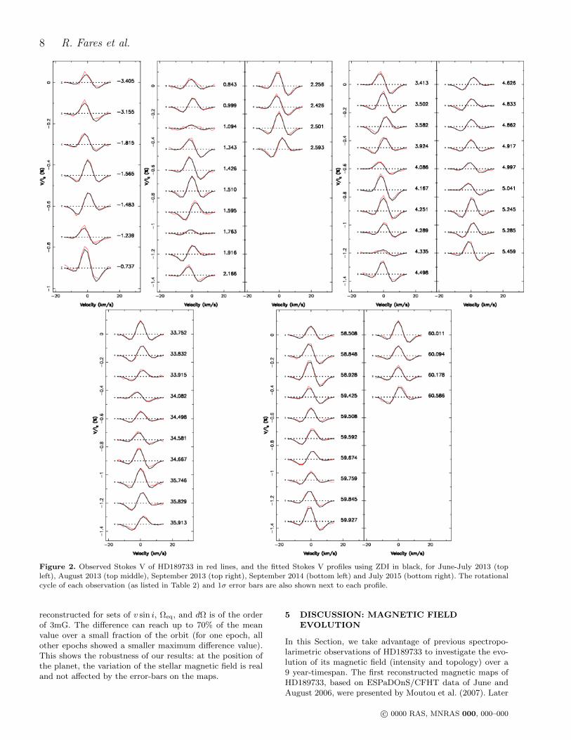
We reconstruct the magnetic maps for five observing epochs.The observed Stokes V (in red) and a 1-sigma error-bar areshown in Fig 2, along with the ZDI reconstructed circularpolarisation (in black). The observed profiles show a detec-tion of the polarisation signature (false-alarm probabilityless than 10−5, see Donati et al. (1997) for the classifica-tion of the detections). The reconstructed maps are shownin Fig 3. As mentioned previously, each dataset used to re-construct a magnetic map consisted of no more than twostellar rotations.

• June/July 2013

We reconstructed the map of June/July 2013, althoughour phase coverage is not optimal. The χ2

r of the recon-struction is 1.15. The mean magnetic field is of 36 G. 61%of the magnetic energy is in the toroidal component. Forthe poloidal component, we define axisymetric modes ashaving m = 0 and m<l/2 (m and l being the order andthe degree of the associated Legendre polynomial, used todescribe the field as spherical harmonics expansion). About40% of the poloidal field is axisymetric.

• August 2013

For August 2013, the data samples the stellar rotationwell. However, the Null profile shows a systematic signaturein the core of the profile. Fitting these Null profiles with nomagnetic field configuration leads to a χ2

r of 1.3. We calcu-lated a mean profile for all the Null profiles. Subtracting themean Null profile from the August 2013 Null spectra leadsto a χ2

r of 0.7 when fitting the corrected Null profiles withno magnetic configuration. Given that the signatures in theNull profiles show a systematic trend, it is more likely to bea spurious signature rather than an underestimation of theerror bars. We subtract the mean Null profile signature ofthe Stokes V profiles. The map is reconstructed with a χ2

r

c© 0000 RAS, MNRAS 000, 000–000

The evolving magnetic field of HD189733 7

of 1.85. The average surface magnetic field is 40 G. 50% ofthe total energy is in the toroidal component of the field.2% of the poloidal energy is in the axisymetric modes, andmainly in modes with m = 0. The poloidal component isthus mainly non-axisymetric. Spherical harmonics modeswith l>3 (i.e. modes higher than the dipole, quadrupoleand octupole) contribute to ∼ 38% of the poloidal energy.

• September 2013

In September 2013, we have data from ESPaDOnS andNARVAL, covering two stellar rotations. We reconstructed amap using those data with a χ2

r of 2.15. We notice a system-atic difference in the Intensity profile depth between Narval’sspectra and ESPaDOnS’ spectra. The difference in depth isnot significant enough to require different modelling of theintensity profiles between instruments. This difference is dueto the normalisation of the spectra at the telescope.

The average surface magnetic field is 42 G. 59% of theenergy in the toroidal component. The poloidal field is stillmainly non-axisymetric (88%, see Table 4). About 50% ofthe poloidal component is in the octupolar mode, higherorders contribute to ∼ 45%.

• September 2014

In September 2014, the average magnetic field drops to31 G (see Fig 3). The χ2

r of the fit is 1.25. The field remainsmainly toroidal, with 78% of the total energy stored inthe toroidal components. The poloidal field is stronglynon-axisymetric, and only 12% of the energy lies withinaxisymmetric modes.

• July 2015

In July 2015, the magnetic field, and in particular theradial component, has changed significantly relative toSeptember 2014. The radial component changes polarityaround the equator between September 2014 and July 2015.The poloidal component contributes to 15% of the total en-ergy. The average magnetic field is of 37 G.

The characteristics of each reconstructed map are listed inTable 4. ZDI does not provide error bars for the recon-structed map. However, statistical errors can be calculatedby varying the input parameters (e.g., v sin i, stellar incli-nation, Ωeq, dΩ) within their error bars. Error bars on fieldcharacteristics are calculated by comparing the characteris-tics of the reconstructed field for the best set of input param-eters to the characteristics of maps reconstructed by varyingthose best input parameters within their error bars. We fol-low Mengel et al. (2016) for error bar calculations: we fix(Ωeq,dΩ) and vary v sin i within its error bars (2.75 km s−1

to 3.2 km s−1, Table 1). We then do a new set of maps fixingv sin i and varying (Ωeq, dΩ) within their error bars. Errorbars in table 4 represent the highest values of our procedure.

4.3 Extrapolation of the magnetic field toinvestigate the corona and the planetary orbit

The interactions between the stellar wind and the planetarymagnetosphere might trigger planetary emission, such as ra-dio emission or bow shock formation (see, e.g. Fares et al.2010; Llama et al. 2013), and it might influence the ionisa-

tion state of the planetary atmosphere (Rimmer & Helling2013; Rimmer, Helling & Bilger 2014). In this Section, weexamine the stellar magnetic field in the corona up to theplanetary orbit using a potential field extrapolation of thesurface magnetic field. For this purpose, we use the Poten-tial Field Source surface (PFSS) code of Jardine, CollierCameron & Donati 2002, originally developed for the Sun(van Ballegooijen et al. 1998) based on Altschuler & Newkirk(1969). The potential field extrapolation assumes that thereis no electric current in the corona. The components of mag-netic field in the corona are described using a spherical har-monics decomposition. This technique delivers satisfactoryresults when compared to wind modelling of the solar corona(Riley et al. 2006).

The PFSS model extrapolates the magnetic field consid-ering two boundary conditions: the first one being that thefield is purely radial at a surface called the Source Surface,the second boundary condition is the observed field geom-etry at the surface of the star. We assume that the SourceSurface is at 3.4 R?. Our radial magnetic maps are used asa boundary condition at the surface of the star, thus givinga realistic model of the radial field.

The extrapolated field in the stellar corona for the fivemaps presented in this paper are shown in Fig 4. This figureshows how different surface field configurations produce dif-ferent field line configuration in the corona. Since the mag-netic field lines in the corona are not those of a very simpleconfiguration, and since the planet and the star are not syn-chronised, the planet crosses different field configuration onits orbit, as well as from one orbit to the other (the planetcrosses in front of the same stellar field configuration af-ter one beat period (of rotation and orbital periods), ratherthan after one orbital period). We calculate, for each observ-ing epoch, the footprints of field lines connecting the stellarsurface to the position of the planet on its orbit . They areshown in Fig 5.

The PFSS model allows the calculation of the field valueand orientation at each position in the corona, out to theSource Surface. Since the planet is outside the Source Sur-face, we proceed as follows to calculate the field at its po-sition. First, we calculate the position of the sub-planetarypoint on the Source Surface, we then calculate the energybudget at this point. We remind the reader here that at theSource Surface, the stellar field is purely radial, the merid-ional and azimuthal components are negligible. Assumingthat the magnetic flux is conserved over spherical shells fromthe source surface to the planetary orbit, we calculate thedecay of the magnetic field between the Source Surface andthe orbit. In Fig 6, we plot the field value at the plane-tary orbit for each epoch of observations (including June2007 and July 2008). The maximum value the field reachesat the planetary orbit can change by 100% between differ-ent epochs, which supports the importance of simultaneousobservations when studying Star-Planet Interactions. We in-vestigate the effect the error bars on the maps could have onthe calculated magnetic field at the planetary orbit. To doso, for each epoch, we use as boundary condition each of themaps calculated for a range of v sin i, Ωeq, and dΩ (see Sec-tion 4.2), extrapolate the magnetic field for each map, andcalculate the magnetic field at the position of the planet. Wefind that the mean difference between the field values pre-sented in this paper and those calculated for the the maps

c© 0000 RAS, MNRAS 000, 000–000

8 R. Fares et al.

Figure 2. Observed Stokes V of HD189733 in red lines, and the fitted Stokes V profiles using ZDI in black, for June-July 2013 (top

left), August 2013 (top middle), September 2013 (top right), September 2014 (bottom left) and July 2015 (bottom right). The rotationalcycle of each observation (as listed in Table 2) and 1σ error bars are also shown next to each profile.

reconstructed for sets of v sin i, Ωeq, and dΩ is of the orderof 3mG. The difference can reach up to 70% of the meanvalue over a small fraction of the orbit (for one epoch, allother epochs showed a smaller maximum difference value).This shows the robustness of our results: at the position ofthe planet, the variation of the stellar magnetic field is realand not affected by the error-bars on the maps.

5 DISCUSSION: MAGNETIC FIELDEVOLUTION

In this Section, we take advantage of previous spectropo-larimetric observations of HD189733 to investigate the evo-lution of its magnetic field (intensity and topology) over a9 year-timespan. The first reconstructed magnetic maps ofHD189733, based on ESPaDOnS/CFHT data of June andAugust 2006, were presented by Moutou et al. (2007). Later

c© 0000 RAS, MNRAS 000, 000–000

The evolving magnetic field of HD189733 9

Figure 3. The reconstructed maps of HD 189733 for June-July 2013 (top row) August 2013 (second row), September 2013 (third row),

September 2014 (fourth raw) and July 2015 (bottom row). The maps are in a polar flattened projection down to latitudes of −30, the

equator is represented by the bold circle. The radial, azimuthal and meridional field components are shown. The magnetic flux valuesare labelled in G. Radial ticks around each map indicate the rotational phase of our observations.

c© 0000 RAS, MNRAS 000, 000–000

10 R. Fares et al.

Figure 4. The extrapolated magnetic field of HD 189733 for June-July 2013 (top left), August 2013 (top middle), September 2013 (topright), September 2014 (bottom left) and July 2015 (bottom right). White lines correspond to the closed magnetic lines, blue ones to

the open field lines (reaching the source surface). The star is shown at the same rotational phase (0.5) to better visualise the differencesin magnetic field topology at each observing epoch. The star is viewed almost equator on (∼ 5), the inclination of the system on thesky (as seen from Earth).

on, and with the aim of detecting star-planet interactionsignatures, Fares et al. (2010) presented two additional re-constructed magnetic maps of HD189733, based on spec-tropolarimetric observations of June 2007 and July 2008, aswell as an update of the reconstructed map of 2006, mergingJune and August data as one dataset.

The data presented in this Paper (5 observing epochsspanning two years) shows that the field of HD 189733 canevolve over a few stellar rotations. Combining datasets span-ning more than two stellar rotations systematically reducesthe quality of the fit. Fares et al. (2010) have merged data

obtained in 2006, spread over 5 stellar rotations. We revis-ited the summer 2006 data and found that the map wasoverfitted. We adopt the results of Moutou et al. (2007) inthis paper.

Due to the 5-year gap in the observations, we can notinvestigate the presence of cyclic variations in the stellarmagnetic field, in a similar way as those reported for theplanet-hosting star τ Boo (Donati et al. 2008; Fares et al.2009, 2013). Nevertheless, an evolution in the stellar mag-netic field intensity and topology can be seen. Variationsin both the axisymmetric contribution to the poloidal field

c© 0000 RAS, MNRAS 000, 000–000

The evolving magnetic field of HD189733 11

Figure 5. The radial magnetic field of HD 189733 for June-July 2013 (top left), August 2013 (top right), September 2013 (middle

left), September 2014 (middle right) and July 2015 (bottom). White dots represent the footprints of the field lines connecting the stellar

surface to the position of the planet on its orbit.

and the toroidal contribution to the total field are observedduring this time span (see Fig 7).

For all epochs (apart from June 2006), the toroidalcomponent dominates over the poloidal one. Petit et al.(2008) suggest, studying a sample of solar-like stars, thatthe toroidal energy dominates over the poloidal one for starswith rotation periods less than ∼ 12 days. HD 189733, hav-ing an equatorial rotation period of 12 days, does not contra-dict their findings. On the other hand, Donati & Landstreet(2009) suggest that stars with Rossby number (Ro) < 1 de-velop toroidal fields. HD 189733 has a Ro = 0.403 (Vidottoet al. 2014). HD 189733 field’s geometry is therefore com-patible with the geometries observed for stars with similarmasses and Ro numbers. The fraction of axisymmetric fieldis almost always less than 50%.

In addition, it is also interesting to compare the evolu-tion of the stellar magnetic field within the 2013 data sets,that are separated by just 9 rotation periods. We note thatlittle variation was seen for the toroidal component. The per-centage of the contributors (dipole, quadrupole, octupole) tothe poloidal field, on the other hand, has changed. The maincontributor to the field (i.e. azimuthal component) does notchange polarity. The radial component evolved, with nega-tive and positive magnetic features appearing at the surface.

Table 4. Magnetic field characteristics of HD189733 for differ-

ent epochs. The columns are: the epoch of the observations, themean magnetic field at the surface of the star, the percentage of

the toroidal energy relative to the total one, the percentage of

the energy contained in the axisymmetric modes of the poloidalcomponent relative to the poloidal energy, the percentage con-

tribution of the dipolar, quadrupolar and octupolar components

to the poloidal energy, and the mean stellar field at the positionof the planetary orbit (see Section 4.3). Results of 2006 are from

Moutou et al. (2007) and the results of 2007 and 2008 are fromFares et al. (2010). Error bars are calculated as in Mengel et al.(2016), i.e. by varying the input parameters within their error

bars. The error bar on Borbit is of the order of 3 mG (see text for

more details).

Epoch Bmean Etor Eaxi El=1 El=2 El=3 Borbit

(G) % % % % % (mG)

7/2015 37+2−2 85+2

−2 9+2−2 33+5

−2 32+2−4 10+10

−1 18

9/2014 32+2−4 78+3

−5 10+2−7 2110

−6 35+6−2 16+1

−6 33

9/2013 42+2−4 59+1

−4 2+2−1 4+4

−1 3+2−1 49+2

−2 31

8/2013 41+2−5 50+5

−5 2−1 10+5−2 20+5

−1 32+3−2 39

6/2013 36+4−3 61+4

−3 38+1−2 21+1

−1 37+3−3 17+5

−1 30

7/2008 36+1−3 77+3

−3 17+2−7 30+4

−5 26+2−8 12−2 23

6/2007 22−3 57+8 26−5 7+2 33+7 30+2−1 16

8/2006 20 60 10 35 20 13

6/2006 18 35 52 50 36 12

c© 0000 RAS, MNRAS 000, 000–000

12 R. Fares et al.

Figure 6. The stellar magnetic field value at the position of the planetary orbit (at 0.031 au). Different colours represent different epochs

of observation. This plot shows that the planet is in a non-homogeneous environment, and that this environment varies from one epochto the other. The error bar shown here is a mean error bar value per orbit, valid for all epochs (see text for more details).

6 CONCLUSIONS AND FUTURE PLANS

This paper is part of the MOVES collaboration (Multiwave-length Observations of an eVaporating Exoplanet and itsStar), which aims to characterise comprehensively the com-plex environment of the exoplanet HD189733b. Orbiting abright and active K dwarf at short distance, this transitinghot-Jupiter has been subjected to many stellar and plan-etary atmosphere studies. The main objectives of MOVESare to probe the different regions of the extended planetaryatmosphere, its interactions with the host-star, and theirtemporal variability. The wider set of multi-wavelength ob-servations (X-ray with Swift and XMM-Newton, UV spec-troscopy with HST and XMM-Newton, and radio observa-tions with LOFAR) were taken contemporaneously with themagnetic field mapping presented here.

In this first paper, we presented a detailed spectropo-larimetric study of HD189733 and studied the evolution ofits magnetism. Stellar magnetism is an important ingre-dient in stellar evolution, and also has important effectson planets surrounding these stars. The star was observed

at five epochs (Jul 2013, Aug 2013, Sept 2013, Sept 2014and Jun 2015), during which we also collected X-ray andUV observations (Wheatley et al, in prep). Using ZeemanDoppler Imaging, we reconstructed the magnetic maps ofthe star. With a strength up to 45 G, the magnetic fieldis dominated by the toroidal component at the five epochs.The toroidal component is mainly axisymmetric during allobserving epochs. In contrast, the poloidal component ismainly non-axisymmetric. We will continue monitoring thissystem to study the magnetic evolution on time-scales longerthan 2 years and look for a potential magnetic cycle. Thesereconstructed magnetic maps are crucial for analysing multi-wavelength observations. They allow us, modelling the stel-lar wind in the corona and at the planetary orbit, to recon-struct the X-ray emission and irradiation of the planet, aswell as the spatial distribution of X-ray that will be absorbedby the extended atmosphere of the exoplanet.

c© 0000 RAS, MNRAS 000, 000–000

The evolving magnetic field of HD189733 13

Figure 7. Magnetic field evolution of HD189733. From left to right: the square-root of the total magnetic energy, the toroidal energyrelative to the total one, and the energy in the axisymmetric modes of the poloidal component relative to the energy of the poloidal

component. Error bars are calculated as stated in the text.

ACKNOWLEDGMENTS

The authors thank an anonymous referee for their usefulcomments. This work is based on observations obtainedwith ESPaDOnS at the Canada-France-Hawaii Telescope(CFHT) and with NARVAL at the Telescope Bernard Lyot(TBL). CFHT/ESPaDOnS are operated by the NationalResearch Council of Canada, the Institut National des Sci-ences de l’Univers of the Centre National de la RechercheScientifique (INSU/CNRS) of France, and the University ofHawaii, while TBL/NARVAL are operated by INSU/CNRS.We thank the CFHT and TBL staff for their help duringthe observations, and in particular R. Cabanac and P. Pe-tit. We also thank J.-F. Donati and E. Hebrard for usefulcomments on the data analysis. RF acknowledges financialsupport by WOW from INAF through the Progetti Premialifunding scheme of the Italian Ministry of Education, Univer-sity, and Research. VB and AL acknowledge the support ofthe French Agence Nationale de la Recherche (ANR), underprogram ANR-12-BS05-0012 ‘Exo-Atmos’. Part of VB workhas been carried out in the frame of the National Centre forCompetence in Research “PlanetS” supported by the SwissNational Science Foundation (SNSF). V.B. also acknowl-edges the financial support of the SNSF. AAV acknowledgespartial support from an Ambizione Fellowship of the SwissNational Science Foundation. ChH highlights financial sup-port of the European Community under the FP7 by an ERCstarting grant number 257431. P.W. is supported by a STFCconsolidated grant (ST/L000733/7)

REFERENCES

Altschuler M. D., Newkirk G., 1969, Sol. Phys., 9, 131Alvarado-Gomez J. D. et al., 2015, A&A, 582, A38

Augustson K. C., Brown B. P., Brun A. S., Miesch M. S.,Toomre J., 2012, ApJ, 756, 169

Balona L. A., Abedigamba O. P., 2016, MNRAS, 461, 497Barnes J. R., Collier Cameron A., Donati J.-F., JamesD. J., Marsden S. C., Petit P., 2005, MNRAS, 357, L1

Barnes J. R., Haswell C. A., Staab D., Anglada-Escude G.,2016, MNRAS, 462, 1012

Ben-Jaffel L., Ballester G. E., 2013, A&A, 553, A52Berdyugina S. V., Berdyugin A. V., Fluri D. M., PiirolaV., 2011, ApJ, 728, L6

Boisse I., Moutou C., Vidal-Madjar A., Bouchy F., PontF., Hebrard, 2009, A&A, 495, 959

Bott K., Bailey J., Kedziora-Chudczer L., Cotton D. V.,Lucas P. W., Marshall J. P., Hough J. H., 2016, MNRAS,459, L109

Bouchy F. et al., 2005, A&A, 444, L15Bourrier V., Lecavelier des Etangs A., 2013, A&A, 557,A124

Bourrier V. et al., 2013, A&A, 551, A63Brogi M., de Kok R. J., Albrecht S., Snellen I. A. G., BirkbyJ. L., Schwarz H., 2016, ApJ, 817, 106

Cegla H. M., Lovis C., Bourrier V., Beeck B., Watson C. A.,Pepe F., 2016, A&A, 588, A127

Chandrasekhar S., 1961, Hydrodynamic and Hydromag-netic Stability. Clarendon Press, Oxford, U.K.

Cohen O., Kashyap V. L., Drake J. J., Sokolov I. V., Gom-bosi T. I., 2011, ApJ, 738, 166

Collier Cameron A., 2007, Astronomische Nachrichten, 328,1030

Cuntz M., Saar S. H., Musielak Z. E., 2000, ApJ, 533, L151Davis T. A., Wheatley P. J., 2009, MNRAS, 396, 1012Distefano E., Lanzafame A. C., Lanza A. F., Messina S.,Spada F., 2016, A&A, 591, A43

Donati J.-F. et al., 2006, MNRAS, 370, 629Donati J.-F., Landstreet J. D., 2009, ARA&A, 47, 333

c© 0000 RAS, MNRAS 000, 000–000

14 R. Fares et al.

Donati J.-F. et al., 2008, MNRAS, 385, 1179

Donati J.-F., Semel M., Carter B. D., Rees D. E., CollierCameron A., 1997, MNRAS, 291, 658

Ehrenreich D. et al., 2012, A&A, 547, A18

Fares R. et al., 2009, MNRAS, 398, 1383

Fares R. et al., 2010, MNRAS, 406, 409

Fares R., Moutou C., Donati J.-F., Catala C., ShkolnikE. L., Jardine M. M., Cameron A. C., Deleuil M., 2013,MNRAS, 435, 1451

Fossati L. et al., 2010, ApJ, 714, L222

Grießmeier J.-M., Preusse S., Khodachenko M.,Motschmann U., Mann G., Rucker H. O., 2007,Planet. Space Sci., 55, 618

Grießmeier J.-M., Zarka P., Spreeuw H., 2007, A&A, 475,359

Helling C., Jardine M., Diver D., Witte S., 2013,Planet. Space Sci., 77, 152

Ip W.-H., Kopp A., Hu J.-H., 2004, ApJ, 602, L53

Jackson A. P., Davis T. A., Wheatley P. J., 2012, MNRAS,422, 2024

Jardine M., Cameron A. C., 2008, A&A, 490, 843

Jardine M., Collier Cameron A., Donati J.-F., 2002, MN-RAS, 333, 339

Koskinen T. T., Harris M. J., Yelle R. V., Lavvas P., 2013,Icarus, 226, 1678

Lammer H. et al., 2011, Origins of Life and Evolution ofthe Biosphere, 41, 503

Lecavelier Des Etangs A., 2007, A&A, 461, 1185

Lecavelier des Etangs A. et al., 2012, A&A, 543, L4

Lecavelier Des Etangs A. et al., 2010, A&A, 514, A72

Lecavelier Des Etangs A., Sirothia S. K., Gopal-Krishna,Zarka P., 2011, A&A, 533, A50

Llama J., Vidotto A. A., Jardine M., Wood K., Fares R.,Gombosi T. I., 2013, MNRAS, 436, 2179

Louden T., Wheatley P. J., 2015, ApJ, 814, L24

Matsakos T., Uribe A., Konigl A., 2015, A&A, 578, A6

Mengel M. W. et al., 2016, MNRAS, 459, 4325

Mengel M. W. et al., 2017, MNRAS, 465, 2734

Morin J. et al., 2008a, MNRAS, 390, 567

Morin J. et al., 2008b, MNRAS, 390, 567

Moutou C. et al., 2007, A&A, 473, 651

Murray-Clay R. A., Chiang E. I., Murray N., 2009, ApJ,693, 23

Petit P. et al., 2008, MNRAS, 388, 80

Pillitteri I., Wolk S. J., Cohen O., Kashyap V., KnutsonH., Lisse C. M., Henry G. W., 2010, ApJ, 722, 1216

Poppenhaeger K., Schmitt J. H. M. M., Wolk S. J., 2013,ApJ, 773, 62

Preusse S., Kopp A., Buchner J., Motschmann U., 2005,A&A, 434, 1191

Reiners A., 2006, A&A, 446, 267

Reiners A., 2012, Living Reviews in Solar Physics, 9, 1

Reiners A., Schmitt J. H. M. M., 2002, A&A, 384, 155

Reinhold T., Reiners A., Basri G., 2013, A&A, 560, A4

Riley P., Linker J. A., Mikic Z., Lionello R., Ledvina S. A.,Luhmann J. G., 2006, ApJ, 653, 1510

Rimmer P. B., Helling C., 2013, ApJ, 774, 108

Rimmer P. B., Helling C., Bilger C., 2014, InternationalJournal of Astrobiology, 13, 173

Rimmer P. B., Stark C. R., Helling C., 2014, ApJ, 787, L25

Scandariato G. et al., 2013, A&A, 552, A7

See V., Jardine M., Fares R., Donati J.-F., Moutou C.,2015, MNRAS, 450, 4323

Shkolnik E., Bohlender D. A., Walker G. A. H., CollierCameron A., 2008, ApJ, 676, 628

Shkolnik E., Walker G. A. H., Bohlender D. A., 2003, ApJ,597, 1092

Shulyak D., Reiners A., Seemann U., Kochukhov O.,Piskunov N., 2014, A&A, 563, A35

Smith A. M. S., Collier Cameron A., Greaves J., JardineM., Langston G., Backer D., 2009, MNRAS, 395, 335

Triaud A. H. M. J. et al., 2009, A&A, 506, 377van Ballegooijen A. A., Nisenson P., Noyes R. W., LofdahlM. G., Stein R. F., Nordlund A., Krishnakumar V., 1998,ApJ, 509, 435

Vidal-Madjar A., Lecavelier des Etangs A., Desert J.-M.,Ballester G. E., Ferlet R., Hebrard G., Mayor M., 2003,Nature, 422, 143

Vidotto A. A., Fares R., Jardine M., Donati J.-F., OpherM., Moutou C., Catala C., Gombosi T. I., 2012, MNRAS,423, 3285

Vidotto A. A., Fares R., Jardine M., Moutou C., DonatiJ.-F., 2015, MNRAS, 449, 4117

Vidotto A. A. et al., 2014, MNRAS, 441, 2361Vidotto A. A., Jardine M., Helling C., 2010, ApJ, 722, L168Vidotto A. A., Opher M., Jatenco-Pereira V., GombosiT. I., 2009, ApJ, 703, 1734

Winn J. N. et al., 2007, AJ, 133, 1828Winn J. N. et al., 2006, ApJ, 653, L69Zarka P., 2007, Planet. Space Sci., 55, 598

c© 0000 RAS, MNRAS 000, 000–000