Mountain permafrost distribution modeling using ... · Mountains (Li et al., 2009), on the eastern QTP. However, in nature logistic regression it still uses a linear function of the

http://www.scar.ac.cn

Sciences in Cold and Arid Regions 2012, 4(5): 0361–0370

DOI: 10.3724/SP.J.1226.2012.00361

Mountain permafrost distribution modeling using Multivariate Adaptive Regression Spline (MARS) in the Wenquan area

over the Qinghai-Tibet Plateau

XiuMin Zhang 1, ZhuoTong Nan 1,2*, JiChun Wu 1, ErJi Du 2, Tong Wang 1, YanHui You 1

1. State Key Laboratory of Frozen Soil Engineering, Cold and Arid Regions Environmental and Engineering Research Institute, Chinese Academy of Sciences, Lanzhou, Gansu 730000, China

2. Cold and Arid Regions Environmental and Engineering Research Institute, Chinese Academy of Sciences, Lanzhou, Gansu 730000, China

*Correspondence to: Dr. ZhuoTong Nan, Professor of Cold and Arid Regions Environmental and Engineering Research Insti-tute, Chinese Academy of Sciences. No. 320, West Donggang Road, Lanzhou, Gansu 730000, China. Tel: +86-931-4967236; Email: [email protected]

Received: March 20, 2012 Accepted: June 27, 2012

ABSTRACT

In high mountainous areas, the development and distribution of alpine permafrost is greatly affected by macro- and mi-cro-topographic factors. The effects of latitude, altitude, slope, and aspect on the distribution of permafrost were studied to under-stand the distribution patterns of permafrost in Wenquan on the Qinghai-Tibet Plateau. Cluster and correlation analysis were per-formed based on 30 m Global Digital Elevation Model (GDEM) data and field data obtained using geophysical exploration and borehole drilling methods. A Multivariate Adaptive Regression Spline model (MARS) was developed to simulate permafrost spa-tial distribution over the studied area. A validation was followed by comparing to 201 geophysical exploration sites, as well as by comparing to two other models, i.e., a binary logistic regression model and the Mean Annual Ground Temperature model (MAGT). The MARS model provides a better simulation than the other two models. Besides the control effect of elevation on permafrost distribution, the MARS model also takes into account the impact of direct solar radiation on permafrost distribution. Keywords: permafrost distribution model; Multivariate Adaptive Regression Splines; Qinghai-Tibet Plateau; permafrost

1. Introduction

Permafrost is a geological entity that has evolved as a result of an exchange of matter and energy between the Earth and atmosphere with multiple impacts of regional geographic conditions, geologic structure, lithology, hy-drology, and topographic characteristics. Permafrost is sensi-tive to environmental changes (Cheng and Zhao, 2000). The characteristics and distribution of permafrost in cold regions seriously affect the stability of embankment engineering constructions (Li et al., 2009); thus, an accurate survey and mapping of permafrost distribution are critical to designing and planning any engineering construction. The traditional method of mapping permafrost is mainly based on field survey data with the map completed by professional people

indoors (Guo et al., 1981; Stocker-Mittaz et al., 2002). Thus, the traditional method requires much labor and time. With the development of Geographical Information System (GIS) and Remote Sensing (RS), a number of permafrost distribu-tion models have been developed for different regions at different spatial scales. Theoretically, permafrost distribution models can be catalogued into two groups: process-oriented models and empirical-statistical models (Hoelzle et al., 2001). Process-oriented models involve a more detailed physical representation of energy fluxes between atmosphere and per-mafrost, for example, PERMEBAL (Lunardini, 1998; Smith and Riseborough, 1998; Hoelzle et al., 2001), PERMACLIM (Guglielmin et al., 2003), and the one-dimensional permafrost evolution model (Li et al., 1996). On the other hand, empiri-cal-statistical models do not consider the process of energy

XiuMin Zhang et al., 2012 / Sciences in Cold and Arid Regions, 4(5): 0361–0370

362

exchange and the specific mechanism between atmosphere and permafrost in detail (Julián and Chueca, 2007). In recent years, empirical-statistical models have been used exten-sively, for example, PERMAKART (Keller, 1992; Imhof, 1996), PERMAMOD (Frauenfelder et al., 1998), equivalent latitude model (Jorgenson and Kreig, 1988), direct radiation model (Funk and Hoelzle, 2006), frost index model (Nelson and Outcalt, 1987; Anisimov and Nelson, 1996; Nelson and Anisimov, 2006), TTOP (Riseborough, 2002; Juliussen and Humlum, 2007), BTS (Ishikawa and Hirakawa, 2000; Isaksen et al., 2002; Antoni and Ednie, 2004; Hoelzle, 2006; Riseborough et al., 2008), and a logistic regression derivation (Jason, 2005; Li et al., 2009).

In China, permafrost is distributed mainly on the Qing-hai-Tibet Plateau (QTP) and the Da- and Xiao-Hinggan mountains. The former is the highest permafrost underlain area in low-latitude regions, with a permafrost area of 1.5×106 km2 (Zhou et al., 2000). Due to physically harsh environmental conditions, such as high elevation, low air temperature, large diurnal temperature range, and strong solar radiation on the QTP, it is extremely hard to collect survey data. The data condition can not sufficiently support process-oriented models. By contrast, empirical-statistical models, such as the elevation model (Cheng and Wang, 1982; Cheng, 1984), equivalent elevation model (Sheng et al., 2010), and Mean Annual Ground Temperature model (MAGT) (Wu et al., 2000, 2001; Nan et al., 2002) have been used extensively in this area.

Previous studies have indicated that latitude, longitude, and elevation are the main factors governing the develop-ment and distribution of permafrost on the QTP (Wu et al., 2000; Zhou et al., 2000; Nan et al., 2002). In high-latitude areas with extensive permafrost distribution, for example, in the Alps, Scandinavia, Japan, Spain, and Canada, elevation and solar radiation contribute importantly to the develop-ment and distribution of alpine permafrost (Gruber and Hoelzle, 2001; Heggem et al., 2005; Etzelmüller et al., 2006; Julián and Chueca, 2007). Similarly, when we study the permafrost distribution on the high elevated QTP, not only the controlling factors but also the local factors which may greatly affect solar radiation, should be taken into account.

In terms of methodology, linear regression methods were used to analyze the spatial distribution of permafrost, as-suming a linear relationship exists between permafrost oc-currence and environmental factors. However, the relation-ship is naturally nonlinear, so statistical methods based on such relationships can hardly produce an accurate perma-frost distribution map. Another form of regression method, the Logistic Regression method (LR), has been used to sim-ulate the spatial distribution of permafrost in the Qilian Mountains (Li et al., 2009), on the eastern QTP. However, in nature logistic regression it still uses a linear function of the predictors to model the probability of outcome.

The Multivariate Adaptive Regression Spline model (MARS) is a non-linear, non-parametric regression method, with a generalization capability specifically for strong high-

dimensional data, proposed by the statistician Jerry Friedman (Friedman, 1991). Since the 1990s, MARS has been used widely and successfully for predictive and simulation efforts, such as land cover classification (Quirós et al., 2009), fire responses to changing climate (Balshi et al., 2008), and spe-cies distribution (Leathwick et al., 2005; Elith and Leathwick, 2007). MARS is better suited to model situations that include a number of variables, non-linearity, multicollinearity, and/or a high degree of interaction among predictors (Munoz and Feli-cisimo, 2004). However, so far, MARS is rarely used to study permafrost distribution, although it looks suitable as permafrost existence is a result of comprehensive effects of climatic conditions and geographical factors.

This study aims to evaluate the effects on the distribution of permafrost of macro- and micro-factors which are select-ed using statistical cluster and correlation analysis. The Wenquan area of the eastern QTP is used as the study area where MARS is used to predict its spatial distribution pat-terns of permafrost. Finally, the simulations from MARS and two other models, namely, the LR and MAGT models, are evaluated. This study shows that MARS presents more advantages on its applicability in mapping permafrost dis-tribution on the QTP. 2. Study area

Wenquan is located in the southeastern part of the QTP. Administratively, it extends across the four counties of Xing-hai, Maduo, Dulan, and Maqin, which belong to the Hainan Tibetan Autonomous Prefecture and the Guoluo Tibetan Au-tonomous Prefecture in Qinghai Province, western China (Figure 1a). Elevations in the study area range from 3,430 m to 5,300 m above sea level, with an average of 4,327 m. Two high and steep mountain ranges, the Ela and Jiangluling mountains, are situated in the study area in a north-west–southeast direction. The Qing-Kang Road traverses through the area in a northeast–southwest direction. There are two basins, the Wenquan Basin and the Kuhai Basin, with lower elevations and flat terrains (Figure 1b). The nearby me-teorological Huashixia station reports average annual temper-ature of −3.2 °C and annual precipitation between 500 and 600 mm (Chou et al., 2009). According to a field investiga-tion in 2009, the study region is dominated by alpine grass-land, meadow, and swamp meadow, and smaller areas of alpine shrub. Alpine meadow and alpine swamp meadow are mainly distributed in low mountains and water-filled depression areas. Alpine grassland is distributed mainly in the high plains. Alpine shrubs are distributed mainly in the northern slopes of Ela and Jiangluling mountains where evaporation and solar radiation intensity are weak.

Wenquan is a typical transition area between permafrost and seasonally frozen soil on the QTP. Permafrost investiga-tions in this region had been conducted during the period of reconstruction of the Qing-Kang Road in the 1990s and 2004, providing information in regards to the distribution and characteristics of permafrost in this region.


363

Figure 1 Location map of the study area (a) and sampling plot locations (b)

3. Data processing 3.1. Data and processing methods

A field investigation, being one of a series of ongoing permafrost surveys on the QTP, has been carried out in Wenquan from September 12 to October 20, 2009. Ground Penetrating Radar (GPR) and borehole drilling were used in this survey. About 130 transects with 626 sampling points were set with an interval of 2 m along transects for the GPR method. The coordinates and elevations of points were rec-orded with a portable GPS. GPR was used to gather perma-frost information during the survey. Data were collected using the Common Offset and Common Midpoint methods. According to the information obtained from GPR in combi-nation with expertise, the depth of permafrost table and the lower elevation limit of permafrost could be determined approximately. Besides, 21 boreholes were drilled in this region (Figure 1b) to verify the performance of the GPR method. Elevation, latitude and longitude, borehole depth, permafrost table, surface conditions, and soil properties about every borehole were recorded in detail. Both GPR and drilling methods provide necessary data to support this study.

Topographic parameters, including elevation, slope, as-pect, and curvatures, on the surveyed locations and the entire area were computed from a 30 m resolution Advanced Spaceborne Thermal Emission and Reflection Radiometer (ASTER) Global Digital Elevation Model (GDEM) provid-ed by the International Scientific Data Service Platform, using the surface analysis procedure from ARCGIS. Solar radiation was calculated using Solar Analyst, an extension to ArcView GIS 3.2 (Fu and Rich, 1999). Solar Analyst takes into account influences of latitude, elevation, slope, surface orientation, shadows cast by surrounding topography, daily and seasonal shifts in solar angle, and atmospheric attenua-tion. With this model, potential direct short-wave solar radi-ation (PSR) over each month, each season, and the whole year of 2009 was calculated every 0.5 hour using 32 horizon

directions (Li et al., 2009). 3.2. Cluster and correlation analyses

The 2 m interval between points was much closer than that necessary for permafrost detection and might bring un-necessary redundancy. A cluster analysis is needed to select points that are more representative. Cluster analysis assigns a set of objects into groups (called clusters) so that the ob-jects in the same cluster are more similar (in some sense or another) to each other than to those in other clusters. The Q type cluster analysis was used and the nearest neighbor method was chosen to analyze a total of 647 points (from GPR and drilling) with 425 sample points remaining after cluster analysis.

One or several factors may play dominant roles in perma-frost occurrence. To analyze the linear association of perma-frost with local factors, a binary state representing permafrost presence (1) or non-presence (0) was set. Screened data from 425 points were analyzed, and the results are presented in Table 1. The most significant relationship was found between the binomial existence of permafrost and elevation with a correlation coefficient of 0.35 at the 0.01 level, showing a strong positive correlation between elevation and permafrost presence. A higher altitude means higher possibility of per-mafrost existence. In low-latitude regions elevation becomes dominant for affecting permafrost distribution. PSR was shown to have a negative significant relation with perma-frost existence (at significance level of 0.01). This finding was consistent with the knowledge that direct incident radia-tion and soil temperature are significantly positively corre-lated. The higher the potential of solar radiation is, the high-er the permafrost temperature is. Because PSR for June on the QTP was the highest, a near zero correlation coefficient with permafrost occurrence can be observed. The other factors, namely, curvature, plan curvature, profile curvature, latitude, longitude, aspect, and slope show no significant relation with permafrost existence (at significance level of 0.05).


364


365

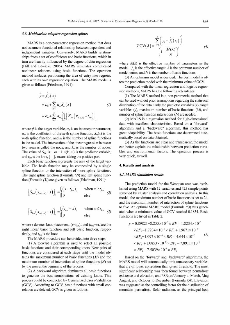
3.3. Multivariate adaptive regression splines

MARS is a non-parametric regression method that does not assume a functional relationship between dependent and independent variables. Conversely, MARS builds relation-ships from a set of coefficients and basic functions, which in turn are heavily influenced by the degree of data regression (Hill and Lewicki, 2006). MARS simulates complicated nonlinear relations using basic functions. The operation method includes partitioning the area of entry into regions, each with its own regression equation. The MARS model is given as follows (Friedman, 1991):

( )

( )

( )( )

01

0 ,1 1

m

M

M

m mm

kM

m km kmv k mm k

f x

x

y

a a S

a a S x t

∧ ∧

=

= = +

=

= +

⎡ ⎤= + −⎣ ⎦

∑

∑ ∏

(1)

where ŷ is the target variable, a0 is an interceptor parameter, am is the coefficient of the m-th spline function, Sm(x) is the m-th spline function, and m is the number of spline functions in the model. The intersection of the linear regression between two areas is called the node, and km is the number of nodes. The value of Skm is 1 or −1. v(k, m) is the predictor variable, and tkm is the knot, [ ]+ means taking the positive part.

Each basic function represents the area of the target var-iable. The basic function may be composited by a single spline function or the interaction of more spline functions. The right spline function (Formula (2)) and left spline func-tion (Formula (3)) are given as follows (Friedman, 1991):

( ) ( )( , )

when

0 elsekm km

km v k m

x t x tS x t +

+

⎧ − ≥⎪⎡ ⎤− = ⎨⎣ ⎦ ⎪⎩ (2)

( ) ( )( , )

when

0 elsekm km

km v k m

t x x tS x t +

+

⎧ − ≤⎪⎡ ⎤− = ⎨⎣ ⎦ ⎪⎩ (3)

where t denotes knot placement, (x−tkm)+ and (tkm−x)+ are the right linear basic function and left basic function, respec-tively, and tkm is the knot.

The MARS procedure can be divided into three steps: (1) A forward algorithm is used to select all possible

basic functions and their corresponding knots. New pairs of functions are considered at each stage until the model ob-tains the maximum number of basic functions (M) and the maximum number of interaction of spline functions (N) set by the user at the beginning of the process.

(2) A backward algorithm eliminates all basic functions to generate the best combinations of existing knots. This process could be conducted by Generalized Cross-Validation (GCV). According to GCV, basic functions with small cor-relation are deleted. GCV is given as follows:

( )( )

2

12GCV

( )1

N

i ii

y f x

MN

λ

λλ

∧

=

⎛ ⎞−⎜ ⎟⎝ ⎠=⎛ ⎞−⎜ ⎟⎝ ⎠

∑ (4)

where M(λ) is the effective number of parameters in the model, is the effective target, λ is the optimum number of model terms, and N is the number of basic functions.

(3) An optimum model is decided. The best model is of-ten the prediction model with the minimum value of GCV.

Compared with the linear regression and logistic regres-sion methods, MARS has the following advantages:

(1) The MARS method is a non-parametric method that can be used without prior assumptions regarding the statistical distribution of the data. Only the predictor variables (x), target variables (y), maximum number of basic functions (M), and number of spline function interactions (N) are needed.

(2) MARS is a regression method for high-dimensional data with excellent characteristics. Based on a "forward" algorithm and a "backward" algorithm, this method has great adaptability. The basic functions are determined auto-matically based on data obtained.

(3) As the functions are clear and transparent, the model can better explain the relationship between prediction varia-bles and environmental factors. The operation process is very quick, as well. 4. Results and analysis 4.1. MARS simulation results

The prediction model for the Wenquan area was estab-lished using MARS with 12 variables and 425 sample points screened by cluster analysis and correlation analysis. In this model, the maximum number of basic functions is set to 24, and the maximum number of interaction of spline functions to five. An optimal MARS model (Formula (5)) was gener-ated when a minimum value of GCV reached 0.1834. Basic functions are listed in Table 2.

3 71

6 62 3

6 74 5

6 97

98 9

0.89821+8.255 10 1.8234 10

1.7234 10 1.9671 10

+1.097 10 4.644 10

1.0853 10 7.8911 10

7.5039 106

y BF

BF BF

BF BF

BF BF

BF BF

− −

− −

− −

− −

−

= × × − ×

× − × × + ×

× × × − ×

× + × × − ×

× + × ×

(5)

Based on the "forward" and "backward" algorithms, the MARS model will automatically omit unnecessary variables that are of lower correlation than given threshold. The most significant relationship was then found between permafrost existence and elevation, and PSRs of January to March, May, August, and October to December (Formula (5)). Elevation was suggested as the controlling factor for the distribution of mountain permafrost. Solar radiation, as the principal heat

f̂λ


366

source of land surface, is another factor affecting distribution of permafrost, especially in cold seasons (September to next April). In winter, snow coverage will provide large reflectiv-ity and reduce thermal absorption. The number of days with negative radiation has a close relationship to permafrost existence.

The PSRs were computed using ArcGIS Solar Analyst. Together with elevation, PSRs were input to Formula (5), where the threshold to determine permafrost was set to 0.5 (Quirós et al., 2009). A value of y ≥0.5 represents permafrost underlain, whereas others represent a seasonally frozen soil type (Figure 2).

4.2. Model validation

The model was validated using 5-fold cross-validation. All 425 sample points were randomly divided into five parts, where four parts, namely 340 sample points, were used for calibration and the remaining one part, namely 85 points, for validation. This model can produce overall accuracies of 78%, 80%, 72%, 72%, and 81%, and an average of 76.6%. Same cross validation was applied to logistic regression method and MAGT model. The logistic regression method (Sheng et al., 2010) is 74.0% in overall accuracy which is smaller than MARS, indicating the latter has a better simulation.

Table 2 Basic functions used in the MARS model

No. Basic function Variable(s) Coefficient BF1 max(0, 4237−x1) Ele 8.255×10−3

BF2 max(0, x3−51891) × max(0, 4389−x1) PSR2, Ele −1.8234×10−7 BF3 BF1 × max(0, 91394−x9) PSR10, Ele −1.7234×10−6 BF4 BF1 × max(0, x7−178030) PSR8, Ele 1.9671×10−6 BF5 BF1 × max(0, 178030−x7) PSR8, Ele 1.097×10−6 BF6 BF1 × max(0, x2−46864) PSR1, Ele −4.644×10−7 BF7 BF1 × max(0, 46864−x2) PSR1, Ele 1.0853×10−6 BF8 max(0, x6−181200) × max(0, 43398−x11) PSR5, PSR12 −7.8911×10−9 BF9 max(0, x6−181200) × max(0, 121240−x4) PSR5, PSR3 7.5039×10−9

Ele: Elevation; PSRn: The potential direct incoming solar radiation of n month.

Figure 2 Permafrost distribution map of the studied area simulated with the MARS model

4.3. Comparison with LR and MAGT

The LR and MAGT models were used to simulate per-mafrost distribution in the Wenquan area of interest. At pre-sent, the MAGT model is a widely-used empirical-statistical

linear model of permafrost distribution (Nan et al., 2002; Heggem et al., 2005; Etzelmüller et al., 2006), derived from borehole measured sub-surface temperature data. Apart from the linear method, there is a non-linear statistical method, such as the nonlinear logistic regression method that was


367

used to simulate permafrost distribution in the eastern Qilian Mountains (Li et al., 2009). We also applied LR and MAGT and compared them to MARS.

For comparative purposes, a binary logistic regression method was used with same data that passed cluster and correlation analyses, among which 253 sample points are of permafrost type and 172 of seasonally frozen soil type. A stepwise regression method was used to screen independent variables that contribute less to the dependent variable. Formula (6) shows the final form of LR taking elevation as the independent variable. By input of the 30 m GDEM data, the probability of permafrost spatial distribution in the Wenquan area was calculated. The threshold is set to 0.5, i.e., a value of P ≥0.5 indicates a permafrost type, and the other values indicate seasonally frozen soil type (Li et al., 2009). The simulated map is presented in Figure 3b.

30.621 0.007

30.621 0.007

e1 e

dem

demP− + ×

− + ×=+

(6)

According to the MAGT model (Nan et al., 2002), the dependent variable is mean annual ground temperatures at the 10 m depth (MAGT) of 21 drilling boreholes, whereas independent variables include latitude, longitude and eleva-tion. Also, a stepwise regression method was used to screen independent variables that are of less correlation to the de

pendent variable. The final MAGT model takes MAGT as the dependent variable and elevation as the independent variable (Formula (7)). The model was then simulated based on the 30 m resolution GDEM data. A MAGT of 0.5 °C is set to the threshold value to distinct permafrost and seasonal frozen soil types (Nan et al., 2002), where MAGT ≤0.5 °C is of permafrost type (Figure 3c).

20.0066 27.8343 0.9731T x r= − + = (7) where T is the predicted mean annual ground temperature of permafrost (°C), and x corresponds to elevation (m), r2 re-lates to the determination coefficient.

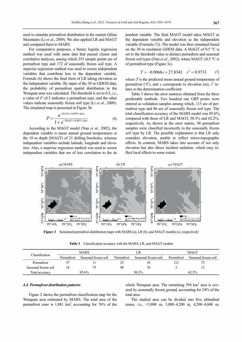
Table 3 shows the error matrices obtained from the three predictable methods. Two hundred one GRP points were entered as validation samples among which, 115 are of per-mafrost type and 86 are of seasonally frozen soil type. The total classification accuracy of the MARS model was 85.6%, compared with those of LR and MAGT, 50.3% and 62.2%, respectively. As shown in the error matrix, 90 permafrost samples were classified incorrectly to the seasonally frozen soil type by LR. The possible explanation is that LR only considers elevation, unable to reflect micro-topographic effects. In contrast, MARS takes into account of not only elevation but also direct incident radiation, which may re-flect local effects to some extent.

Figure 3 Simulated permafrost distribution maps with MARS (a), LR (b), and MAGT models (c), respectively

Table 3 Classification accuracy with the MARS, LR, and MAGT models

Classification MARS LR MAGT

Permafrost Seasonal frozen soil Permafrost Seasonal frozen soil Permafrost Seasonal frozen soilPermafrost 97 11 25 10 112 73

Seasonal frozen soil 18 75 90 76 3 13 Total accuracy 85.6% 50.3% 62.2%

4.4. Permafrost distribution patterns

Figure 2 shows the permafrost classification map for the Wenquan area estimated by MARS. The total area of the permafrost zone is 1,881 km2, accounting for 76% of the

whole Wenquan area. The remaining 594 km2 area is cov-ered by seasonally frozen ground, accounting for 24% of the total area.

The studied area can be divided into five altitudinal zones, i.e., <3,800 m, 3,800–4,200 m, 4,200–4,600 m,


368

4,600–5,000 m, and >5,000 m. 1.81% of total studied area is distributed in the lowest elevation zone, mainly in the Wen-quan valley. There is 24.34% of total area in the 3,800 m to 4,200 m altitudinal zone, which covers southeast to north-east directional mountains and the Kuhai Basin. The altitu-dinal zone from 4,200 m to 4,600 m accounts for 61.14% of the total area, including the Maritang Basin, and the low elevation regions of the Ela and Jiangluling mountains. The zone with elevation from 4,600 m to 5,000 m, includ-ing the middle mountain parts of the Ela and Jiangluling mountains, accounts for 12.55% of the total area. The zone with elevation higher than 5,000 m accounts for about 0.16% of the total area, including high mountain areas (Figure 4a).

In terms of altitudinal distribution characteristics, per-mafrost is extensively distributed throughout high, medium, and low mountain zones, that is to say it is mainly concen-trated in the Ela and Jiangluling mountains. Moreover, per-mafrost covers 71.35%, 44.50%, 82.86%, 98.86%, and 97.58% of each altitudinal zones, respectively, i.e., <3,800 m, 3,800–4,200 m, 4,200–4,600 m, 4,600–5,000 m, and >5,000 m (Figure 4b). By comparison, seasonally frozen soils are distributed in the medium and low mountainous regions, including the Daheba and Wenquan valleys, the Kuhai Basin and the Maritang Plain. For each altitudinal zone, seasonally frozen soil covers 28.65%, 55.50%, 7.14%, 1.14%, and 2.42% of the zonal area, respectively (Figure 4b).

As presented in Figures 2 and 4b, the main factor con-

trolling permafrost development is elevation. However, as a micro-climatic factor, PSR also influences the distribution of permafrost at a much smaller scale. Generally speaking, the amount of solar radiation largely depends on geographic latitude. However, for a small area, solar radiation is also determined by varying topographic conditions such as slope, aspect, and land surface conditions.

In summer, vegetation serves as a canopy shield that re-duces incoming solar radiation to the ground surface. Whereas in cold seasons, with the plateau vegetation going into senescence, more negative heat flux directly enters the soil in favor of permafrost development. These effects are insignificant in the southeastward areas and in the Maritang Plain. However, in some southeast alpine areas permafrost can occur in lower altitudes. This fact may be related to steep slope that prevents surface solar radiation entering into the ground. In northern slopes, alpine shrub and alpine swamp meadow are well established because of favorable water conditions, which considerably reduce solar radiation. As vegetation evapotranspiration also consumes radiation, less heat goes into the ground which is beneficial to the de-velopment of permafrost. That is why we find permafrost coverage in a much lower elevation. For the same reason, in high elevations in the Maritang Plain and the Kuhai Basin, seasonally frozen soil is fully developed because of relative-ly flat topography and sparse alpine grassland coverage. Abundant solar radiation is adverse to permafrost formation in those areas.

Figure 4 Altitudinal zones of the studied area (a) and percentages of permafrost and seasonally frozen soil in different altitudinal zones calculated using MARS (b)

Considering the simulations from the three different

methods, they have similar seasonally frozen soil and per-mafrost distribution characteristics, with seasonally frozen soil mainly distributed in the 3,400–4,200 m altitudinal range and permafrost mostly in the zone higher than 4,200 m. All simulations come to the same conclusion that eleva-tion dominates permafrost distribution in this studied area. However, due to the difference of methods, distribution var-

iations still can be found among them. The simulations of LR and MAGT models show that permafrost is lacking be-low 3,800 m and no seasonally frozen soil exists higher than 4,600 m. However, the MARS model shows that both per-mafrost and seasonally frozen soil can be distributed in all elevations (Table 4). This can be contributed to a compre-hensive consideration of not only elevation but also implicit local factor effects of slope, aspect and surface conditions,


369

which make MARS better in representing alpine complexity and local effects. Statistically, as presented in Tables 3 and 4, an analysis of classification accuracy estimates of the three methods confirms the outstanding performance of MARS. 5. Conclusion

Using measured permafrost distribution information from in-field borehole and GPR investigations, a MARS based model was established for permafrost distribution

simulation in the Wenquan area. The following conclusions were drawn.

(1) Comparing MARS, MAGT, and LR methods using the same dataset, MARS produces a most accurate simula-tion. All models confirm that elevation is the dominant fac-tor to control macro-distribution patterns of regional perma-frost. The simulation variations are related to local factors that affect the micro-distribution of permafrost, which can be taken into account implicitly by introducing potential solar radiation in the MARS model.

Table 4 Areal percentages of permafrost and seasonal frozen soil in different altitudinal zones simulated with different models

Altitudinal zones (m) MARS MAGT LR

Permafrost Seasonal frozen soil Permafrost Seasonal frozen soil Permafrost Seasonal frozen soil3,400–3,800 71.35% 28.65% 0 100% 0 100% 3,800–4,200 44.50% 55.50% 30.97% 69.03% 0 100% 4,200–4,600 82.86% 17.14% 100% 0 60.72% 39.28% 4,600–5,000 98.86% 1.14% 100% 0 100% 0 ≥5,000 97.58% 2.42% 100% 0 100% 0

(2) On the basis of MARS simulation in the studied area,

permafrost covers about 1,881 km2 area, which is mainly distributed in altitudes higher than 4,200 m, accounting for 76% of the total area. In addition, most seasonally frozen soil is distributed in altitudes from 3,400 to 4,200 m. Acknowledgments: This research was supported financially by the Special Basic Research Program of China (Grant No. 2008FY110200) and partially by Open Programme of State Key Laboratory (No. SKLFSE201009). Field investigation was carried out by the State Key Laboratory of Frozen Soil Engineering and State Key Laboratory of Cryospheric Science of CAREERI/CAS. We would like to thank the International Scientific Data Service Platform, which provided the 30m-GDEM data covering the study area. Many thanks should go to Dr. Yu Sheng, Dr. Lin Zhao, Dr. Ji Chen and Dr. Jing Li for their helps in carrying out the field investigations and obtaining valuable data. REFERENCES Anisimov OA, Nelson FE, 1996. Permafrost distribution in the Northern

Hemisphere under scenarios of climatic change. Global and Planetary Change, 14(1–2): 59–72.

Antoni GL, Ednie M, 2004. Probability mapping of mountain permafrost using the BTS method, Wolf Creek, Yukon Territory, Canada. Permafrost and Periglacial Processes, 15(1): 67–80.

Balshi MS, Mcguire AD, Duffy P, Flannigan M, Walsh J, Melillo J, 2008. Assessing the response of area burned to changing climate in western boreal North America using a Multivariate Adaptive Regression Splines (MARS) approach. Global Change Biology, 15(3): 578–600.

Cheng GD, 1984. Problems on zonation of high altitude permafrost. Journal of Geographical Science, 39(2): 185–193.

Cheng GD, Wang SL, 1982. On the zonation of high altitude permafrost in China. Journal of Glaciology and Geocryology, 4(2): 12–16.

Cheng GD, Zhao L, 2000. The problems associated with permafrost in the development of the Qinghai-Xizang Plateau. Quaternary Sciences, 20(6):

521–531. Chou YL, Sheng Y, Wei ZM, 2009. Temperature and deformation differ-

ences between southern and northern slopes of highway embankment on permafrost. Chinese Journal of Rock Mechanics and Engineering, 28(9): 1896–1903.

Elith J, Leathwick J, 2007. Predicting species distributions from museum and herbarium records using multiresponse models fitted with multivariate adaptive regression splines. Diversity and Distributions, 13(3): 265–275.

Etzelmüller B, Heggem ESF, Sharkhuu N, Frauenfelder R, 2006. Mountain permafrost distribution modelling using a multi-criteria approach in the Hövsgöl Area, Northern Mongolian. Permafrost and Periglacial Process-es, 17: 91–104.

Frauenfelder R, Allgwer B, Haeberli W, 1998. Permafrost investigations with GIS on a case study in the Fletschhorn area, Wallis, Swiss Alps. PERMAFROST. Proceedings of the Seventh International Conference, Yellow knife (Canada), Collection Nordicana No. 55, pp. 291–295.

Friedman J, 1991. Multivariate adaptive regression splines. The Annals of Statistics, 19(1): 1–67.

Fu P, Rich P, 1999. Design and implementation of the Solar Analyst: an ArcView extension for modeling solar radiation at landscape scales. Proceedings of the Nineteenth Annual ESRI User Conference. San Diego, USA.

Funk M, Hoelzle M, 2006. A model of potential direct solar radiation for investigating occurrences of mountain permafrost. Permafrost and Peri-glacial Processes, 3(2): 139–142.

Gruber S, Hoelzle M, 2001. Statistical modeling of mountain permafrost distribution: Local calibration and incorporation of remotely sensed data. Permafrost and Periglacial Processes, 12(1): 69–77.

Guglielmin M, Aldighieri B, Testa B, 2003. PERMACLIM: a model for the distribution of mountain permafrost, based on climatic observations. Geomorphology, 51(4): 245–257.

Guo DX, Wang SL, Lu GW, Dai JB, Li EY, 1981. Regionalization of perma-frost in the Da and XiaoXing’anling Mountains in northeastern China. Journal of Glaciology and Geocryology, 3(3): 1–9.

Heggem ESF, Juliussen H, Etzemüller B, 2005. The permafrost distribution in Central-Eastern Norway. Norsk Geografisk Tidskrift, 59(2): 94–108.

Hill T, Lewicki P, 2006. Statistics: Methods and Applications. A Comprehen-sive Reference for Science, Industry and Data Minining. StatSoft, Tulsa, USA.

Hoelzle M, 2006. Permafrost occurrence from BTS measurements and climatic parameters in the Eastern Swiss Alps. Permafrost and Periglacial Processes, 3(2): 143–147.

Hoelzle M, Mittaz C, Etzelmüller B, Haeberli W, 2001. Surface energy fluxes and distribution models of permafrost in European mountain areas: an overview of current developments. Permafrost and Periglacial Pro-


370

cesses, 12: 53–68. Imhof M, 1996. Modeling and verification of the permafrost distribution in

the Bernese Alps (Western Switzerland). Permafrost and Periglacial Pro-cesses, 7(3): 267–280.

Isaksen K, Hauck C, Gudevang E, Rune S, Sollid JL, 2002. Mountain per-mafrost distribution in Dovrefjell and Jotunheimen, southern Norway, based on BTS and DC resistivity tomography data. Norsk Geografisk Tidsskrift—Norwegian Journal of Geography, 56(2): 122–136.

Ishikawa M, Hirakawa K, 2000. Mountain permafrost distribution based on BTS measurements and DC resistivity soundings in the Daisetsu Moun-tains, Hokkaido, Japan. Permafrost and Periglacial Processes, 11(2): 109–123.

Jason RJ, 2005. The occurrence of alpine permafrost in the Front Range of Colorado. Geomorphology, 67(3–4): 375–389.

Jorgenson M, Kreig R, 1988. A model for mapping permafrost distribution based on landscape component maps and climatic variables. PERMAFROST—Fifth International Conference. Tapir Publishers, Tapir. Trondheim. 1: 176–182.

Julián A, Chueca J, 2007. Permafrost distribution from BTS measurements (Sierra de Telera, Central Pyrenees, Spain): assessing the importance of solar radiation in a mid-elevation shaded mountainous area. Permafrost and Periglacial Processes, 18(2): 137–149.

Juliussen H, Humlum O, 2007. Towards a TTOP ground temperature model for mountainous terrain in central-eastern Norway. Permafrost and Peri-glacial Processes, 18(2): 161–184.

Keller F, 1992. Automated mapping of mountain permafrost using the pro-gram PERMAKART within the geographical information system ARC/INFO. Permafrost and Periglacial Processes, 3(2): 133–138.

Leathwick JR, Rowe D, Richardson J, Elith J, Hastie T, 2005. Using multi-variate adaptive regression splines to predict the distributions of New Zealand’s freshwater diadromous fish. Freshwater Biology, 50(12): 2034–2052.

Li J, Sheng Y, Wu JC, Chen J, Zhang XM, 2009. Probability distribution of permafrost along a transportation corridor in the northeastern Qinghai Province of China. Cold Regions Science and Technology, 59(1): 12–18.

Li SX, Cheng GD, Guo DX, 1996. The future thermal regime of numerical simulating permafrost on Qinghai-Xizang (Tibet) Plateau, China, under climate warming. Science in China (Series D), 26(4): 342–347.

Lunardini VJ, 1998. Climatic warming and the degradation of warm perma-frost. Permafrost and Periglacial Processes, 7(4): 311–320.

Munoz J, Felicisimo M, 2004. Comparison of statistical methods commonly used in predictive modeling. Journal of Vegetation Science, 15(2): 285–292.

Nan ZT, Li SX, Liu YZ, 2002. Mean annual ground temperature distribution on the Tibetan Plateau, permafrost distribution mapping and further ap-plication. Journal of Glaciology and Geocryology, 24(2): 142–148.

Nelson FE, Anisimov OA, 2006. Permafrost zonation in Russia under an-thropogenic climatic change. Permafrost and Periglacial Processes, 4(2): 137–148.

Nelson FE, Outcalt SI, 1987. A frost index number for spatial prediction of ground-frost zones. Arctic and Alpine Research, 19: 279–288.

Quirós E, Felicísimo ÁM, Cuartero A, 2009. Testing multivariate adaptive regressionsplines (MARS) as a method of land cover classification of TERRA-ASTER satellite images. Sensors, 9(11): 9011–9028.

Riseborough DW, 2002. The mean annual temperature at the top of perma-frost, the TTOP model, and the effect of unfrozen water. Permafrost and Periglacial Processes, 13(2): 137–143.

Riseborough DW, Shiklomanov N, Etzelmüller B, Gruber S, Marchenko S, 2008. Recent advances in permafrost modelling. Permafrost and Perigla-cial Processes, 19(2): 137–156.

Sheng Y, Li J, Wu JC, Ye BS, Wang J, 2010. Distribution patterns of perma-frost in the upper area of Shule river with the application of GIS tech-nique. Journal of China University of Mining and Technology, 1: 32–39.

Smith MW, Riseborough DW, 1998. Permafrost monitoring and detection of climate change. Permafrost and Periglacial Processes, 7(4): 301–309.

Stocker-Mittaz C, Hoelzle M, Haeberli W, 2002. Modelling alpine perma-frost distribution based on energy-balance data: a first step. Permafrost and Periglacial Processes, 13(4): 271–282.

Wu QB, Li X, Li WJ, 2000. Computer simulation and mapping of the re-gional distribution of permafrost along the Qinghai-Xizang highway. Journal of Glaciology and Geocryology, 22(4): 323–325.

Wu QB, Li X, Li WJ, 2001. The response model of permafrost along the Qinghai–Tibetan highway under climate change. Journal of Glaciology and Geocryology, 23(1): 1–6.

Zhou YW, Guo DX, Qiu GQ, 2000. Geocryology in China. Press of Science, Beijing, pp. 40–46.

Documents

Mountain permafrost distribution modeling using ... · Mountains (Li et al., 2009), on the eastern QTP. However, in nature logistic regression it still uses a linear function of the