Motivation - People | UBC's Okanagan campus ounda ries. Using Kelo wna's natural exp eriment to investigate some of these issues. John Janmaat Green with La wn Envy Background Mo del

BackgroundModelResultsConclusionReferencesGreen with Lawn Envy: Spatial Variation of WaterDemand in Kelowna, British ColumbiaJohn Janmaat11Department of EconomicsUniversity of British Columbia - Okanagan CampusKelowna, British Columbia, Canadapresented at Université du Québec a MontréalJohn Janmaat Green with Lawn Envy

BackgroundModelResultsConclusionReferencesOutline1 BackgroundMotivationLiterature2 ModelData SourcesSummariesModel3 ResultsDiagnostic TestsRegression Results: SummerRegression Results: WinterPrediction: Summer4 Conclusion John Janmaat Green with Lawn Envy

BackgroundModelResultsConclusionReferences MotivationLiteratureOutline1 BackgroundMotivationLiterature2 ModelData SourcesSummariesModel3 ResultsDiagnostic TestsRegression Results: SummerRegression Results: WinterPrediction: Summer4 Conclusion John Janmaat Green with Lawn Envy

BackgroundModelResultsConclusionReferences MotivationLiteratureMotivationRole of price in water demand management.Role of education and other e�orts.Do peer in�uences matter?Five water providers in Kelowna.Di�erent rate structures and information campaignsAreas with similar housing across service area boundaries.Using Kelowna's natural experiment to investigate some ofthese issues. John Janmaat Green with Lawn Envy

BackgroundModelResultsConclusionReferences MotivationLiteratureGeography

John Janmaat Green with Lawn Envy





BackgroundModelResultsConclusionReferences MotivationLiteratureKelowna Water Providers


BackgroundModelResultsConclusionReferences MotivationLiteratureOutline1 BackgroundMotivationLiterature2 ModelData SourcesSummariesModel3 ResultsDiagnostic TestsRegression Results: SummerRegression Results: WinterPrediction: Summer4 Conclusion John Janmaat Green with Lawn Envy

BackgroundModelResultsConclusionReferences MotivationLiteratureLiteratureWater demand analysis [Arbués et al., 2003, Dalhuisen et al.,2003, Worthington and Ho�man, 2008]Generally focus on price and other variablesDemand for water price inelastic, less so for discretionary uses.Spatial issues in water consumption analysisStatistically signi�cant neighbourhood di�erences [Aitkenet al., 1991, Troy and Holloway, 2004].Geographically weighted regression [Wentz and Gober, 2007].Exploring spatial structure [Franczyk and Chang, 2009,Ramachandran, 2010***]John Janmaat Green with Lawn Envy

BackgroundModelResultsConclusionReferences MotivationLiteratureLiteraturePatterns in residential landscapingYes [Zmyslony and Gagnon, 1998, Henderson et al., 1998,Zmyslony and Gagnon, 2000].No [Kirkpatrick et al., 2009].Attitudes and intentions [Iverson Nassauer et al., 2009].Spatial econometrics�Spatial Econometrics: Methods and Models [Anselin, 1988].�Being applied broadly now [Anselin et al., 2004, Arbia andBaltagi, 2009, LeSage and Pace, 2009].Spatial water use analysis new.John Janmaat Green with Lawn Envy

BackgroundModelResultsConclusionReferences Data SourcesSummariesModelOutline1 BackgroundMotivationLiterature2 ModelData SourcesSummariesModel3 ResultsDiagnostic TestsRegression Results: SummerRegression Results: WinterPrediction: Summer4 Conclusion John Janmaat Green with Lawn Envy

BackgroundModelResultsConclusionReferences Data SourcesSummariesModelSourcesWater Use Records: City of KelownaGIS addresses and property boundaries: City of KelownaPeter Lomas (RA) generated relevant variables from GIS layersProperty characteristics: LandcorTM, BC Assessment Authority



BackgroundModelResultsConclusionReferences Data SourcesSummariesModelSeasonal Water UseM

onth

ly W

ater

Use

(m3 )

1999

Jan

1999

Jul

2000

Jan

2000

Jul

2001

Jan

2001

Jul

2002

Jan

2002

Jul

2003

Jan

2003

Jul

2004

Jan

2004

Jul

2005

Jan

2005

Jul

2006

Jan

2006

Jul

2007

Jan

2007

Jul

2008

Jan

2008

Jul

050

100

150

200

All Q1 Q2 Q3 Q4John Janmaat Green with Lawn Envy

BackgroundModelResultsConclusionReferences Data SourcesSummariesModelSpatial Water UseWinter

Okana

gan

Lake

Q1Q2Q3Q4

Summer

Okana

gan

Lake

Q1Q2Q3Q4John Janmaat Green with Lawn Envy

BackgroundModelResultsConclusionReferences Data SourcesSummariesModelKelowna North


BackgroundModelResultsConclusionReferences Data SourcesSummariesModelCrawford Estates


BackgroundModelResultsConclusionReferences Data SourcesSummariesModelBinary and Categorical VariablesS

hare

of S

ampl

e

AllQ1Q2Q3Q4

0.0

0.1

0.2

0.3

0.4

0.5

Pool

PrimeV

iew

GoodV

iew

FairV

iew

Wat

erfro

nt

a) Binary

Bathrooms

1 2 3 4 5 6+

b) Bathrooms

Bedrooms

1 2 3 4 5 6 7

c) Bedrooms

Aspect

N E S W

d) Aspect


BackgroundModelResultsConclusionReferences Data SourcesSummariesModelStandardized Continuous Variables−

0.2

−0.

10.

00.

10.

2

Lot S

ize

Finish

ed A

rea

Impr

oved

Asses

smen

t Tota

l

Asses

smen

t

Year

Buil

t

Effecti

ve Ye

arSlop

e

Elevat

ionJohn Janmaat Green with Lawn Envy


BackgroundModelResultsConclusionReferences Data SourcesSummariesModelModelSpatial Autoregressive Moving Average~y = ρW1~y +X~β +~u~u = λW2~u+~εSpatial autoregressive model, W2 = 0.Spatial lag model, W1 = 0SARMA (spatial autoregressive moving average), W1 6= 0 andW2 6= 0.Two dimensional autoregressive process in OLS model.John Janmaat Green with Lawn Envy

BackgroundModelResultsConclusionReferences Data SourcesSummariesModelSpatial Weights: Neighboursk nearest neighbour (k = 4)Each observation has same number of neighboursSphere of in�uenceFind distance to nearest neighbours, diDraw circle radius di around each observation.Neighbours are points where circles touch.Distance boundInclude as neighbours all points within distance bound(d ∈ {50,100,200}m)John Janmaat Green with Lawn Envy

BackgroundModelResultsConclusionReferences Data SourcesSummariesModelSpatial Weights: WeightingsIn�uence of distanceEqual In�uence (distance ignored)Inverse DistanceInverse Distance SquaredRow standardizationScale rows of weighting matrix to sum one.Required for some algorithms.Implicit assumption that observations have same totalin�uence on neighbours, and only distribution of that in�uencevaries.May overstate impact of observations with few neighbours (espat edge). John Janmaat Green with Lawn Envy

BackgroundModelResultsConclusionReferences Data SourcesSummariesModelRe�ection Problem [Manski, 1993]An identi�cation problemCauses of observed spatial correlationsContextual: similar exogenous variables in neighbourhoodCorrelated: unobserved local correlated shocksEndogenous: mimicing local peersIn linear model,Contextual identi�able with Durbin model~y = ρW~y +X~β +WX~θ +~ε

~θ 6= 0, contextual e�ect.ρ 6= 0, endogenous (peer) and/or correlated e�ects.John Janmaat Green with Lawn Envy

BackgroundModelResultsConclusionReferences Data SourcesSummariesModelRe�ection ProblemIn linear model,Correlated and endogenous separate with di�erence model forpanel dataRequire variation in exogenous variables over time, orendogenous confounded with contextCurrent data inadequate


BackgroundModelResultsConclusionReferences Data SourcesSummariesModelEstimation and PredictionEstimation Equation~ε = (I −λW )(I −ρW )~y− (I −λW )X~βKnown distribution, ML, but di�cult inversionUnknown distribution, GMMPrediction Equation

~y = (I −ρW )−1X~β +(I −ρW )−1(I −λW )−1~εIn�uence of changes in ~β and ~ε propagate across allobservations. John Janmaat Green with Lawn Envy

BackgroundModelResultsConclusionReferences Diagnostic TestsRegression Results: SummerRegression Results: WinterPrediction: SummerOutline1 BackgroundMotivationLiterature2 ModelData SourcesSummariesModel3 ResultsDiagnostic TestsRegression Results: SummerRegression Results: WinterPrediction: Summer4 Conclusion John Janmaat Green with Lawn Envy

BackgroundModelResultsConclusionReferences Diagnostic TestsRegression Results: SummerRegression Results: WinterPrediction: SummerDiagnostic TestsMoran's I, common test for spatial relations.Does not identify type of structure.Lagrange multiplier testsSpatial lag, robust to presence of spatial error.Spatial error, robust to spatial lag.Presence of spatial lag and error.Evaluated for a range of spatial weights matrices.John Janmaat Green with Lawn Envy

BackgroundModelResultsConclusionReferences Diagnostic TestsRegression Results: SummerRegression Results: WinterPrediction: SummerDiagnostic TestsMoran Spatial ErrorWeights θ P θ P λk = 4 18.2 0.0000 21.1 0.0000 0.213k = 8 23.0 0.0000 0.0 0.9217 0.318k = 20 29.8 0.0000 93.5 0.0000 0.456SOI 16.3 0.0000 25.3 0.0000 0.156Spatial Lag SARMAWeights θ P ρ θ P ρ λk = 4 198.6 0.0000 0.392 523.4 0.0000 0.409 -0.232k = 8 230.7 0.0000 0.431 748.5 0.0000 0.443 -0.177k = 20 259.5 0.0000 0.465 1118.1 0.0000 0.467 -0.039SOI 148.6 0.0000 0.337 411.3 0.0000 0.358 -0.199John Janmaat Green with Lawn Envy

BackgroundModelResultsConclusionReferences Diagnostic TestsRegression Results: SummerRegression Results: WinterPrediction: SummerDiagnostic Tests Moran Spatial ErrorWeights θ P θ P λ1/√d200 41.4 0.0000 597.4 0.0000 0.6121/d200 38.1 0.0000 343.0 0.0000 0.5731/d2200 25.5 0.0000 0.1 0.7432 0.3601/√d100 27.7 0.0000 38.2 0.0000 0.4071/d100 26.4 0.0000 12.9 0.0003 0.3821/d2100 21.1 0.0000 11.4 0.0007 0.2791/√d50 11.2 0.0000 1.3 0.2536 0.2281/d50 11.1 0.0000 2.1 0.1436 0.2191/d250 10.3 0.0000 5.1 0.0241 0.185John Janmaat Green with Lawn Envy

BackgroundModelResultsConclusionReferences Diagnostic TestsRegression Results: SummerRegression Results: WinterPrediction: SummerDiagnostic Tests Spatial Lag SARMAWeights θ P ρ θ P ρ λ1/√d200 263.9 0.0000 0.477 1884.3 0.0000 0.467 0.2001/d200 251.3 0.0000 0.487 1663.4 0.0000 0.482 0.1121/d2200 272.4 0.0000 0.479 899.9 0.0000 0.492 -0.1871/√d100 245.8 0.0000 0.467 986.5 0.0000 0.474 -0.1101/d100 229.7 0.0000 0.475 929.3 0.0000 0.484 -0.1571/d2100 251.9 0.0000 0.475 680.4 0.0000 0.497 -0.2731/√d50 54.8 0.0000 0.375 172.2 0.0000 0.394 -0.1931/d50 51.0 0.0000 0.376 172.3 0.0000 0.396 -0.2001/d250 54.7 0.0000 0.346 152.1 0.0000 0.371 -0.188John Janmaat Green with Lawn Envy


BackgroundModelResultsConclusionReferences Diagnostic TestsRegression Results: SummerRegression Results: WinterPrediction: SummerContinuous VariablesOLS SAR LAG SARMAIntercept 2.823∗∗∗ 2.827∗∗∗ 1.437∗∗∗ 1.386∗∗∗Assessed 0.191∗∗∗ 0.217∗ 0.103∗ 0.087∗Assessed2 −0.087∗∗∗ −0.088∗∗∗ −0.069∗∗∗ −0.063∗∗∗Age 0.080∗∗∗ 0.083∗∗∗ 0.056∗∗∗ 0.051∗∗∗Age2 −0.016∗∗∗ −0.015∗∗∗ −0.010∗∗∗ −0.009∗∗∗Lot ha 6.076∗∗∗ 5.605∗∗∗ 3.273∗∗∗ 3.177∗∗∗(Lot ha)2 −10.73∗∗∗ −9.711∗∗∗ −6.126∗∗∗ −6.047∗∗∗Bld ha 0.195∗∗∗ 0.173∗∗∗ 0.137∗∗∗ 0.133∗∗∗(Bld ha)2 −0.019∗∗∗ −0.017∗ −0.012∗ −0.012∗Slope −0.025∗∗∗ −0.024∗∗∗ −0.017∗∗∗ −0.016∗∗∗Elevation 0.916∗∗∗ 1.095∗∗∗ 0.434∗∗∗ 0.386∗∗∗

∗∗∗ P < 0.001 ∗∗ P < 0.01 ∗ P < 0.05 . P < 0.1John Janmaat Green with Lawn Envy

BackgroundModelResultsConclusionReferences Diagnostic TestsRegression Results: SummerRegression Results: WinterPrediction: SummerInteractions and Binary VariablesOLS SAR LAG SARMAAssess×Lot 1.036∗∗∗ 1.028∗∗∗ 0.896∗∗∗ 0.840∗∗∗Assess×Bld 0.014 0.012 0.011 0.012Pool 0.139∗∗∗ 0.124∗∗∗ 0.116∗∗∗ 0.117∗∗∗View 0.013 −0.007 −0.020 −0.010Aspect N −0.047∗∗ −0.045∗∗ −0.047∗∗ −0.044∗∗Aspect S −0.008 −0.015 −0.013 −0.009Aspect W −0.036∗ −0.030. −0.024. −0.025∗Near Agr 0.041. 0.057 0.001 −0.001Near GEID −0.022 −0.026 −0.035 −0.034∗∗∗ P < 0.001 ∗∗ P < 0.01 ∗ P < 0.05 . P < 0.1John Janmaat Green with Lawn Envy

BackgroundModelResultsConclusionReferences Diagnostic TestsRegression Results: SummerRegression Results: WinterPrediction: SummerCategorical VariablesOLS SAR LAG SARMABeds 2 −0.064 −0.072. −0.081. −0.075.Beds 3 0.016 −0.004 −0.024 −0.015Beds 4 0.003 −0.015 −0.032 −0.024Beds 5 0.028 0.010 −0.001 0.007Beds 6 −0.008 −0.025 −0.027 −0.007Beds 7 0.024 0.034 0.051 0.050Beds 8+ −0.197. −0.153 −0.114 −0.126Baths 2 0.114∗∗∗ 0.103∗∗∗ 0.090∗∗∗ 0.089∗∗∗Baths 3 0.162∗∗∗ 0.141∗∗∗ 0.114∗∗∗ 0.116∗∗∗Baths 4 0.163∗∗∗ 0.143∗∗∗ 0.125∗∗∗ 0.127∗∗∗Baths 5 0.155∗∗∗ 0.142∗∗∗ 0.132∗∗ 0.131∗∗Baths 6+ −0.089 −0.083 −0.072 −0.073John Janmaat Green with Lawn Envy

BackgroundModelResultsConclusionReferences Diagnostic TestsRegression Results: SummerRegression Results: WinterPrediction: SummerDiagnostics OLS SAR LAG SARMAλ 0.284 −0.262ρ 0.472∗∗∗ 0.493∗∗∗SSE 2385.4 2269.0 2210.1 2127.4cor(y , y) 0.599 0.626 0.638 0.655R2 0.359 0.391 0.406 0.429n 10995 10995 10995 10995



BackgroundModelResultsConclusionReferences Diagnostic TestsRegression Results: SummerRegression Results: WinterPrediction: SummerContinuous VariablesOLS SAR LAG SARMAIntercept 2.7060∗∗∗ 2.7286∗∗∗ 2.1732∗∗∗ 2.1118∗∗∗Assessed −0.0653. −0.0601 −0.0615 −0.0627Assessed2 −0.0071 −0.0054 −0.0043 −0.0048Age 0.0899∗∗∗ 0.0835∗∗∗ 0.0784∗∗∗ 0.0793∗∗∗Age2 −0.0122∗∗∗ −0.0116∗∗∗ −0.0107∗∗∗ −0.0107∗∗∗Lot ha −0.3232 −0.3797. −0.5173. −0.5114.(Lot ha)2 −0.5230 −0.3958 −0.1405 −0.1510Bld ha 0.1178∗∗∗ 0.1267∗∗∗ 0.1156∗∗∗ 0.1106∗∗∗(Bld ha)2 −0.0081∗ −0.0089. −0.0079. −0.0075.Slope −0.0057∗∗∗ −0.0056∗∗ −0.0050∗∗ −0.0049∗∗Elevation −0.4975∗∗∗ −0.5722∗∗∗ −0.4434∗∗∗ −0.4059∗∗∗

∗∗∗ P < 0.001 ∗∗ P < 0.01 ∗ P < 0.05 . P < 0.1John Janmaat Green with Lawn Envy

BackgroundModelResultsConclusionReferences Diagnostic TestsRegression Results: SummerRegression Results: WinterPrediction: SummerInteractions and Binary VariablesOLS SAR LAG SARMAAssess×Lot 0.6161∗∗∗ 0.6022∗ 0.5798∗ 0.5802∗Assess×Bld −0.0138 −0.0156 −0.0150 −0.0143Pool 0.0773∗∗∗ 0.0795∗∗∗ 0.0767∗∗∗ 0.0752∗∗∗View −0.0302. −0.0297. −0.0306. −0.0306.Aspect N −0.0483∗∗ −0.0438∗ −0.0407∗ −0.0415∗Aspect S 0.0045 0.0023 0.0021 0.0028Aspect W −0.0244. −0.0230 −0.0196 −0.0195Near Agr −0.0245 −0.0299 −0.0261 −0.0237Near GEID −0.0410 −0.0356 −0.0399 −0.0415∗∗∗ P < 0.001 ∗∗ P < 0.01 ∗ P < 0.05 . P < 0.1John Janmaat Green with Lawn Envy

BackgroundModelResultsConclusionReferences Diagnostic TestsRegression Results: SummerRegression Results: WinterPrediction: SummerCategorical VariablesOLS SAR LAG SARMABeds 2 −0.0359 −0.0318 −0.0333 −0.0350Beds 3 −0.0047 0.0026 −0.0026 −0.0060Beds 4 0.0513 0.0546 0.0499 0.0477Beds 5 0.1237∗∗ 0.1292∗ 0.1241∗ 0.1207∗Beds 6 0.1984∗∗∗ 0.1929∗∗ 0.1928∗∗ 0.1937∗∗Beds 7 0.3616∗∗∗ 0.3562∗∗∗ 0.3570∗∗∗ 0.3571∗∗∗Beds 8+ 0.5801∗∗∗ 0.5585∗∗∗ 0.5683∗∗∗ 0.5741∗∗∗Baths 2 0.0670∗∗∗ 0.0688∗∗∗ 0.0641∗∗∗ 0.0626∗∗Baths 3 0.1016∗∗∗ 0.1037∗∗∗ 0.0965∗∗∗ 0.0946∗∗∗Baths 4 0.1286∗∗∗ 0.1271∗∗∗ 0.1221∗∗∗ 0.1216∗∗∗Baths 5 0.2417∗∗∗ 0.2447∗∗∗ 0.2393∗∗∗ 0.2366∗∗∗Baths 6+ 0.0960 0.0863 0.0873 0.0901John Janmaat Green with Lawn Envy

BackgroundModelResultsConclusionReferences Diagnostic TestsRegression Results: SummerRegression Results: WinterPrediction: SummerDiagnostics OLS SAR LAG SARMAλ 0.126 −0.063ρ 0.190 0.209SSE 2302.4 2285.6 2288.2 2280.1cor(y , y) 0.309 0.319 0.318 0.323R2 0.095 0.102 0.101 0.104n 10995 10995 10995 10995



BackgroundModelResultsConclusionReferences Diagnostic TestsRegression Results: SummerRegression Results: WinterPrediction: SummerPrediction and OptimizationPotential to optimally choose location of innovations.E.g. spatially target subsidiesLocation of innovationsWhat is the impact on water saved of di�erent innovationpatterns?Scaling multiple innovationsDo innovations impact each other?Spatial weights matrixWhat is impact of wrong matrix on optimal placement?John Janmaat Green with Lawn Envy

BackgroundModelResultsConclusionReferences Diagnostic TestsRegression Results: SummerRegression Results: WinterPrediction: SummerPrediction and OptimizationImpact of innovations∆~y = (I −ρW )−1(I −λW )−1∆~εInnovations where ∆εi = 1, ∆εj 6=i = 0 with ∑∆εi = k fork = 2 and k = 4.ScalingRaw, ∆~y unchanged.Trimmed, if ∆yi > 1, set ∆yi = 1.Scaled, adjust ∆~y by 1/max(∆~y ).StandardizationRow standardized, all rows sum to one.Matrix standardized, sum of matrix elements equal to numberof rows. John Janmaat Green with Lawn Envy

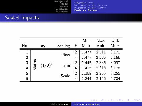
BackgroundModelResultsConclusionReferences Diagnostic TestsRegression Results: SummerRegression Results: WinterPrediction: SummerScaled Impacts Min. Max. Di�.No. wd Scaling k Mult. Mult. Mult.1 Matrix (1/d)2 Raw 2 1.477 2.511 3.1712 4 1.477 2.505 3.1563 Trim 2 1.445 2.386 3.0974 4 1.415 2.318 3.1785 Scale 2 1.389 2.265 3.2556 4 1.244 2.146 4.704John Janmaat Green with Lawn Envy

BackgroundModelResultsConclusionReferences Diagnostic TestsRegression Results: SummerRegression Results: WinterPrediction: SummerScaled Impacts Min. Max. Di�.No. wd Scaling k Mult. Mult. Mult.7 Matrix √1/d Raw 2 1.442 2.628 3.6828 4 1.442 2.618 3.6599 Trim 2 1.420 2.493 3.55410 4 1.420 2.401 3.33511 Scale 2 1.411 2.346 3.27412 4 1.274 2.201 4.377John Janmaat Green with Lawn Envy

BackgroundModelResultsConclusionReferences Diagnostic TestsRegression Results: SummerRegression Results: WinterPrediction: SummerScaled Impacts Min. Max. Di�.No. wd Scaling k Mult. Mult. Mult.13 Row (1/d)2 Raw 2 1.586 2.329 2.26714 4 1.586 2.329 2.26815 Trim 2 1.491 2.257 2.56316 4 1.388 2.256 3.24017 Scale 2 1.338 2.174 3.47218 4 1.112 2.170 10.421John Janmaat Green with Lawn Envy

BackgroundModelResultsConclusionReferences Diagnostic TestsRegression Results: SummerRegression Results: WinterPrediction: SummerScaled Impacts Min. Max. Di�.No. wd Scaling k Mult. Mult. Mult.19 Row √1/d Raw 2 1.505 2.456 2.88320 4 1.505 2.456 2.88321 Trim 2 1.451 2.380 3.06022 4 1.381 2.380 3.61323 Scale 2 1.357 2.283 3.59724 4 1.125 2.277 10.218John Janmaat Green with Lawn Envy

BackgroundModelResultsConclusionReferences Diagnostic TestsRegression Results: SummerRegression Results: WinterPrediction: SummerOptimal Patterns: Minimumsa) 1,3,7,9,11,13,19,21 b) 5,15,17,23 c) 2,8,10,14,20 d) 6,12,16,22


BackgroundModelResultsConclusionReferences Diagnostic TestsRegression Results: SummerRegression Results: WinterPrediction: SummerOptimal Patterns: Maximumsa) 1,7 b) 13,15,17,21,23 c) 3,9 d) 2,8

e) 14,16,18,20,22,24 f) 4,10 g) 6 h) 12


BackgroundModelResultsConclusionReferences Diagnostic TestsRegression Results: SummerRegression Results: WinterPrediction: SummerCost of Being WrongActual wd = (1/d)2 wd =

√1/dMatrix Standard Row Standard Matrix Standard Row StandardRaw Trim Scale Raw Trim Scale Raw Trim Scale Raw Trim Scale1 2 3 4 5 6 7 8 9 10 11 12Assumed1 1.00 0.90 0.76 0.88 0.78 0.68 1.00 0.92 0.82 0.84 0.76 0.702 0.99 1.00 0.99 0.89 0.88 0.88 0.98 1.00 0.99 0.86 0.85 0.853 0.94 0.97 1.00 0.94 0.94 0.95 0.92 0.96 0.99 0.92 0.93 0.934 0.89 0.93 0.96 1.00 1.00 1.00 0.87 0.91 0.95 1.00 1.00 1.005 0.89 0.93 0.96 1.00 1.00 1.00 0.87 0.91 0.95 1.00 1.00 1.006 0.89 0.93 0.96 1.00 1.00 1.00 0.87 0.91 0.95 1.00 1.00 1.007 1.00 0.90 0.76 0.88 0.78 0.68 1.00 0.92 0.82 0.84 0.76 0.708 0.99 1.00 0.99 0.89 0.88 0.88 0.98 1.00 0.99 0.86 0.85 0.859 0.96 0.99 0.99 0.91 0.91 0.91 0.95 0.98 1.00 0.89 0.89 0.8810 0.89 0.93 0.96 1.00 1.00 1.00 0.87 0.91 0.95 1.00 1.00 1.0011 0.89 0.93 0.96 1.00 1.00 1.00 0.87 0.91 0.95 1.00 1.00 1.0012 0.89 0.93 0.96 1.00 1.00 1.00 0.87 0.91 0.95 1.00 1.00 1.00John Janmaat Green with Lawn Envy

BackgroundModelResultsConclusionReferences Diagnostic TestsRegression Results: SummerRegression Results: WinterPrediction: SummerPolicy ImplicationsWhere innovations occur impacts total water savings.Voluntary xeriscaping subsidies may end up concentrated inneighbourhoods with an 'early adopter', rather thanencouraging xeriscaping across the city.Spatially targeted support for conservation may have a greatertotal e�ect.


BackgroundModelResultsConclusionReferencesConclusionStrong evidence for spatial correlation in Kelowna residentialwater use.Summer, spatial lag structure dominantWinter, spatial error structure dominantSpatial structure implies spatial multiplierMultiplier increases with dispersion of innovationsInnovations along edge smaller impact than in centerNo evidence of edge e�ectNeighbour mimicry dominates price?John Janmaat Green with Lawn Envy

BackgroundModelResultsConclusionReferencesFurther WorkThe re�ection problem [Manski, 1993]Spatial correlation from endogenous (peer), correlated, orcontextual e�ects.Durbin Spatial Model~y = ρW~y +X~β +WX~θ +~ε

~θ 6= 0, contextual e�ect.ρ 6= 0, endogenous (peer) and/or correlated e�ects.ML Durbin model supports endogenous (peer) and/orcorrelated e�ects.Di�erence in di�erence with panel to separate.John Janmaat Green with Lawn Envy

BackgroundModelResultsConclusionReferencesFurther WorkIncorporate landscaping detailImage processing of aerial photographs (money?)Street-view assessment of 'degree of xeriscaping'Development historyCaptured by Durbin model?Household characteristicsOther purveyors with potential boundary e�ectsBuild panel dataCurrent variables all constant in one dimension (space or time).John Janmaat Green with Lawn Envy

BackgroundModelResultsConclusionReferencesReferences IC. K. Aitken, H. Duncan, and T. A. McMahon. A cross-sectionalregression analysis of residential water demand in Melbourne,Australia. Applied Geography, 11:157�165, 1991.Luc Anselin. Spatial Econometrics: Methods and Models. Studiesin Operational Regional Science. Kluwer Academic Publishers,1988.Luc Anselin, R.J.G.M Florax, and S.J. Rey, editors. Advances inSpatial Econometrics. Springer, 2004.Guiseppe Arbia and Badi H. Baltagi, editors. Spatial Econometrics:Methods and Applications. Physica-Verlag, Heidelberg, 2009.John Janmaat Green with Lawn Envy

BackgroundModelResultsConclusionReferencesReferences IIFernando Arbués, María Ángeles García-Valiñas, and RobertoMartínez-Espi neira. Estimation of residential water demand: astate-of-the-art review. Journal of Socio-Economics, 32(1):81 �102, 2003.ISSN 1053-5357. doi: DOI:10.1016/S1053-5357(03)00005-2. URLhttp://www.sciencedirect.com/science/article/B6W5H-483BY57-1/2/e1b7bbfa827c3ad935b7298f4feb8cdd.Jasper M. Dalhuisen, Raymond J. G. M. Florax, Henri L. F.deGroot, and Peter Nijkamp. Price and income elasticities ofresidential water demand: A meta-analysis. Land Economics, 79(2):292�308, May 2003.Jon Franczyk and Heejun Chang. Spatial analysis of water use inOregon, usa, 1985�2005. water resources management, 23:755�774, 2009. doi: 10.1007/s11269-008-9298-9.John Janmaat Green with Lawn Envy

http://www.sciencedirect.com/science/article/B6W5H-483BY57-1/2/e1b7bbfa827c3ad935b7298f4feb8cdd

BackgroundModelResultsConclusionReferencesReferences IIIScott P.B. Henderson, Nathan H. Perkins, and Maurice Nelischer.Residential lawn alternatives: a study of their distribution, formand structure. Landscape and Urban Planning, 42:135�145,1998.Joan Iverson Nassauer, Zhifang Wang, and Erik Dayrell. What willthe neighbours think? Cultural norms and ecological design.Landscape and Urban Planning, 92:282�292, 2009.Jamie Kirkpatrick, Grant Daniels, and Aidan Davison. Anantipodean test of spatial contagion in front garden character.Landscape and Urban Planning, 93:103�110, 2009.James LeSage and Robert Kelley Pace. Introduction to SpatialEconometrics. CRC Press, New York, 2009.John Janmaat Green with Lawn Envy

BackgroundModelResultsConclusionReferencesReferences IVCharles F. Manski. Identi�cation of endogenous social e�ects: There�ection problem. The Review of Economic Studies, 60(3):531�542, July 1993.Mahesh Ramachandran. Three Essays in the Economics ofSuburban Water Demand: A Spatial Panel Data Analysis ofResidential Outdoor Water Demand. PhD thesis, ClarkUniversity, 2010.Patrick Troy and Darren Holloway. The use of residential waterconsumption as an urban planning tool: a pilot study inAdelaide. Journal of Environmental Planning and Management,47(1):97�114, 2004.John Janmaat Green with Lawn Envy

BackgroundModelResultsConclusionReferencesReferences VElizabeth A. Wentz and Patricia Gober. Determinants of small-areawater consumption for the city of Phoenix, Arizona. WaterResources Management, 21:1849�1863, 2007. doi:10.1007/s11269-006-91330.Andrew C. Worthington and Mark Ho�man. An empirical survey ofresidential water demand modelling. Journal of EconomicSurveys, 22(5):842 � 871, 2008. ISSN 09500804.Jean Zmyslony and Daniel Gagnon. Residential management ofurban front-yard landscape: A random process? Landscape andUrban Planning, 40:295�307, 1998.Jean Zmyslony and Daniel Gagnon. Path analysis of spatialpredictors of front yard vegetation in an anthropogenicenvironment. Landscape Ecology, 15:375�371, 2000.John Janmaat Green with Lawn Envy

Documents

Motivation - People | UBC's Okanagan campus ounda ries. Using Kelo wna's natural exp eriment to investigate some of these issues. John Janmaat Green with La wn Envy Background Mo del