Motion Tracking for Medical Imaging

Tom Sullivan SCPD

tom.sullivan@kla.com

Sophia Williams Stanford University

sophiarw@gmail.com

Jonathan Fisher Stanford University

jofisher@stanford.edu

Alexander Yoffe SCPD

alexander.yoffe@kla.com

Abstract— Acquisition of medical images (e.g. PET, MRI, etc.) often requires a patient to remain motionless for long periods of time. Even the most compliant patients can’t meet this requirement. Motion compensation methods are used to alleviate this challenge. To compensate for this involuntary movement, one tracks the motion of the patients and incorporates this information into an image reconstruction algorithm. In this paper, we explore three methods of 3D motion tracking of patients using digital images. The three methods are: (1) tracking the motion of an object using two cameras and a geometric target, (2) tracking the motion of an object using one camera and a geometric target, and (3) tracking the motion of an object using two cameras and feature detection algorithms. Our results indicate that methods (1) and (2) may be better suited for robust motion tracking.

Keywords—Medical Imaging, 3D image tracking, stereo tracking, single-image tracking, feature tracking

I. INTRODUCTION (HEADING 1) Positron emission tomography (PET) is a non-invasive

medical imaging modality that provides 3D visualization of physiological processes in a subject’s body. PET complements other medical imaging modalities such as X-ray computed tomography (CT) and magnetic resonance imaging (MRI), which provide high-resolution anatomy, with cellular and molecular information on disease.

The data collected by the PET detector in very noisy. To achieve quantitative image data requires many corrections, including detector efficiency variation correction and photon attenuation correction. For motionless subjects, different methods to estimate and compensate for each degrading factor have been developed. But for imaging of living subjects, there will always be a certain amount of motion that adds another layer of complexity; it causes errors in positioning events along the PET system detector lines of response which leads to significant blurring, inaccurate quantification and additional noise.

To mitigate the problem a motion correction solution is required. The solution shold track the motion and incorporate the information into a suitable image reconstruction algorithm [1], [2].

The most accurate and effective motion tracking approaches in PET/MR scan settings are MR-based [3] and camera-based (provides superior performance), [1], [4], [5], [6].

In this paper we discuss the implementation and compare the results of three different camera-based motion tracking methods for PET motion correction:

1. We track the motion of an object using two cameras and a geometric target.

2. We track the motion of an object using one camera and a geometric target.

3. We track the motion of an object using two cameras and feature detection.

Fig. 1. Typical PET/CT (left) and PET/MRI brain scans of a normal subject acquired separately on the two dual-modality systems.

II. CALIBRATION An essential part of 3D image reconstruction is finding the

mapping from 2D image space to 3D space. This mapping is defined by the matrix 𝑀 which is a product of the intrinsic matrix, 𝐾, and the extrinsic matrix, [𝑅|𝑇]. 𝐾 is consists of the internal properties of the camera, such as focal length, principal point offset (center of array). [𝑅|𝑇]is the combination of the rotation and translation of the camera in space. To find these matrices we use the built-in Matlab Application called CameraCalibrator that is based on the popular Zhang calibration method [1]. For stereo camera processing, we calibrate the two cameras independently and we calculate the rotation and translation between cameras. We do this using the Matlab Application called StereoCameraCalibrator.

III. DATA COLLECTION AND GROUND TRUTH Our images are collected using two Logitech C615 web

cameras that interface with Matlab. Each camera has 1080p resolution. The cameras are mounted such that they maintain their positions relative to one another so that we only have to calibrate the cameras once.

The ground truth, or an estimate of the true position in 3D space, is determined using a MicronTracker for tracking algorithms (1) and (2). A MicronTracker is a commercial product that uses stereo images to locate targets in 3D space. The device has a reported accuracy of 0.25mm RMS and an update rate of 48Hz. The performance of our 3D localization is assessed by comparing the outputs of our algorithms to a data set composed of 3 correspondences between the Microntracker and images of the target taken usingour stereo camera set-up.

To assess the performance of our tracking algorithm that uses feature detection we also developed a set of stereo images of a face without a target. The true position of the head was measured using the magnetic tracker, which was attached to the back of the head. The magnetic tracker used is the MagTracker, which has a resolution of 1.4 mm RMS. The magnetic tracker provides more accurate position estimates than measuring the distances manually.

Stereo videos were also taken, with a 20Hz frame rate, with and without a target. These videos are used to assess certain properties of our algorithms, such as their sensitivity to brightness and motion blur.

IV. KEYPOINT IDENTIFICATION Finding the target’s keypoints is a universal first step

required for the first two motion tracking algorithm being discussed in this paper, as it establishes a correspondence between the target geometry and our images. In this chapter, we will describe how we found the 10 key points of the target shown in Fig. 2.

Fig. 2. Example of the target used for tracking in the presented algorithms. The 10 keypoints are labeled in red.

Fig. 3. Example of the target with a green background mounted on a tripod.

Fig. 4. Example of a target identified using our target segmentation algorithm.

A. Target Segmentation The first step was to segment the target from the rest of the

image. To simplify this part, we choose to give the target a green background, as shown in Fig. 3.

To segment the target we took the following steps, we:

1. Convert the image to color space (CIE 1976 L*a*b* values)

2. Perform k-means in opponent color space (a*, b*) and find the color that is closest to the target color (was found empirically) (the method worked for several sets of images with different lighting conditions) Fig. 5(a).

3. Isolate the biggest segment and perform morphological image processing so that the segmented part will be bigger than the actual target Fig. 5(c) and (b).

4. Perform locally adaptive thresholding using Otsu’s method on the segmented pixels of the gray image Fig. 5(c) and (d).

A zoomed in version of the final result is presented in Fig. 4.

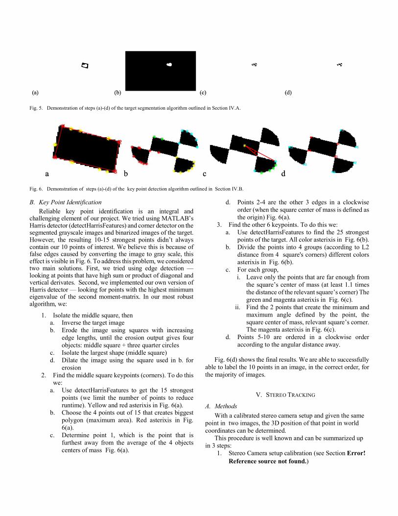
Fig. 5. Demonstration of steps (a)-(d) of the target segmentation algorithm outlined in Section IV.A.

Fig. 6. Demonstration of steps (a)-(d) of the key point detection algorithm outlined in Section IV.B.

B. Key Point Identification Reliable key point identification is an integral and

challenging element of our project. We tried using MATLAB’s Harris detector (detectHarrisFeatures) and corner detector on the segmented grayscale images and binarized images of the target. However, the resulting 10-15 strongest points didn’t always contain our 10 points of interest. We believe this is because of false edges caused by converting the image to gray scale, this effect is visible in Fig. 6. To address this problem, we considered two main solutions. First, we tried using edge detection — looking at points that have high sum or product of diagonal and vertical derivates. Second, we implemented our own version of Harris detector — looking for points with the highest minimum eigenvalue of the second moment-matrix. In our most robust algorithm, we:

1. Isolate the middle square, then a. Inverse the target image b. Erode the image using squares with increasing

edge lengths, until the erosion output gives four objects: middle square + three quarter circles

c. Isolate the largest shape (middle square) d. Dilate the image using the square used in b. for

erosion 2. Find the middle square keypoints (corners). To do this

we: a. Use detectHarrisFeatures to get the 15 strongest

points (we limit the number of points to reduce runtime). Yellow and red asterixis in Fig. 6(a).

b. Choose the 4 points out of 15 that creates biggest polygon (maximum area). Red asterixis in Fig. 6(a).

c. Determine point 1, which is the point that is furthest away from the average of the 4 objects centers of mass Fig. 6(a).

d. Points 2-4 are the other 3 edges in a clockwise order (when the square center of mass is defined as the origin) Fig. 6(a).

3. Find the other 6 keypoints. To do this we: a. Use detectHarrisFeatures to find the 25 strongest

points of the target. All color asterixis in Fig. 6(b). b. Divide the points into 4 groups (according to L2

distance from 4 square's corners) different colors asterixis in Fig. 6(b).

c. For each group, i. Leave only the points that are far enough from

the square’s center of mass (at least 1.1 times the distance of the relevant square’s corner) The green and magenta asterixis in Fig. 6(c).

ii. Find the 2 points that create the minimum and maximum angle defined by the point, the square center of mass, relevant square’s corner. The magenta asterixis in Fig. 6(c).

d. Points 5-10 are ordered in a clockwise order according to the angular distance away.

Fig. 6(d) shows the final results. We are able to successfully

able to label the 10 points in an image, in the correct order, for the majority of images.

V. STEREO TRACKING

A. Methods With a calibrated stereo camera setup and given the same

point in two images, the 3D position of that point in world coordinates can be determined.

This procedure is well known and can be summarized up in 3 steps:

1. Stereo Camera setup calibration (see Section Error! Reference source not found.)

2. Find correspondences between points in left and right cameras (see Section IV).

3. Triangulation which is solved using the linear triangulation method [10].

B. Results To evaluate the accuracy of the results, a comparison with

the MicronTracker output was performed. However, we realized that determining the extrinsic matrix that transformed out camera setup to the MicronTracker coordinate frame was very difficult to measure. This was partly due to the fact that we did not know exactly which point the MicronTracker was using as its origin. So instead of trying to perform an absolute comparison between our outputs and the MicronTracker’s, we opted for a relative comparison between target reference frames. The idea with this approach is that while we cannot get the single camera results to agree absolutely with the MicronTracker results, they should be able to agree on how much the target moved between frames of motion, M1 and M2, using the target’s own reference frame. Stated another way, we are finding the pose of the target after it has been moved, with respect to its own starting reference frame This concept is captured by the following expression,

( 𝑀+,-./0 )2 𝑀+,-/3

. 4 = 𝑀+,-/3/0 = 2 𝑀+,-6789:;

/0 42 𝑀+,-/36789:; 4

Where 𝑀+,-.

/0 and 𝑀+,-6789:;/0 are the inverses of 𝑀+,-/0

. and 𝑀+,-/0

6789:; , respectively. These results are shown below in Table 1 for two different motions.

Table 1 - Pose estimation from target's own frame of reference between motions 1 and 2

Micron Tracker

Two Camera (cherry picked)

|Error|

Two Camera (full algo

run)

|Error|

Θx [rad]

0.05 -0.01 0.06 -0.36 0.41

Θy [rad]

-0.40 -0.43 0.03 0.03 0.43

Θz [rad]

0.06 0.04 0.02 0.02 0.04

tx [mm]

29.58 29.48 0.10 19.25 10.33

ty [mm]

21.69 21.03 0.66 -27.28 48.97

tz [mm]

-11.64 -12.61 0.97 -6.45 5.19

Table 2 - Pose estimation from target's own frame of reference between

motions 1 and 3

Micron Tracker

Two Camera (cherry picked)

|Error|

Two Camera (full algo

run)

|Error|

Θx [rad]

0.13 0.13 0.00 -0.47 0.60

Θy [rad]

-0.48 -0.46 0.02 -0.03 0.45

Θz [rad]

0.04 0.05 0.01 0.03 0.01

tx [mm]

83.38 81.96 1.42 23.84 59.54

ty [mm]

32.84 32.15 0.69 -74.14 106.98

tz [mm]

-93.95 -91.39 2.56 -81.84 12.11

These results suggest this method is very sensitive to noise

in the keypoint location. The cherry picked results are vastly superior to the results produced with segmentation keypoints.

VI. SINGLE CAMERA TRACKING

A. Methods The objective of this method is to estimate the pose, of a

known geometric target using only a single camera. If the pose of the target can be determined for each frame of motion, then the motion of the target is known. The terms model and target will be used interchangeably in this section.

The target used for this method is show in Fig. 2, and the correspondence between keypoints on the target body and their pixel locations is found in the segmentation portion of the algorithm described in IV. In addition to establishing this keypoint correspondence, the intrinsic matrix, K, of the camera must be known, seeSection Error! Reference source not found.Error! Reference source not found.. Lastly, rigid body motion of the target is assumed.

The algorithm to be discussed utilizes the principle of perspective projection. Equation (1) describes this operation. The notation convention being used is leading superscripts represent the frame in which the object or action is observed [9].

𝑝. = 𝑲( 𝑹/. 𝑡/:9@. ) 𝑃/ (1)

Where C𝑝 is the projected point in the camera reference frame, 𝑹/. is the rotation of the model reference frame as seen in the camera reference frame, 𝑡/:9@. is the translation of the model origin as seen in the camera reference frame, and 𝑃/ is the point in the model’s reference frame. The term ( 𝑹/. 𝑡/:9@. ) is referred to as the extrinsic matrix, 𝑴𝒆𝒙𝒕.

Finally, to convert C𝑝toscreenpixels,itisconvertedtohomogeneouscoordinatesbydividingeachtermbythe“z”term.

𝑝. = _𝑥𝑦𝑧c,𝑥76d@+ = 𝑥 𝑧⁄ , 𝑦76d@+ = 𝑦 𝑧⁄ (2)

In the above two equations, both the model keypoints ( 𝑃/ ) and the screen points (𝑥76d@+, 𝑦76d@+) are known, along with the camera intrinsic matrix. The unknown is the extrinsic matrix, which encodes the pose information of the target in the camera’s frame of reference. The following gradient descent algorithm was employed to iteratively solve for the pose [1].

1. Make an initial guess for the pose of the form 𝑥 =(𝜃, 𝜃h 𝜃i 𝑡, 𝑡h 𝑡i)j . Here the first three terms represent rotations about the x, y, and z axes, respectively. The last three terms are the translation components, also referred to as 𝑡/:9@. .

2. Project the target keypoint coordinates onto screen-space using equation (1) and (2). Compare the error between these projected points and the known keypoint locations in screen-space.

3. If the error is less than some threshold, calculate the Jacobian of the projection operation (f(x)), 𝐽 =𝜕𝑓 𝜕𝑥⁄ , and evaluate at x. This produces the relationship 𝑑𝑦 = 𝐽𝑑𝑥

4. Solve for 𝑑𝑥 using the pseudo inverse, 𝑑𝑥 =(𝐽j𝐽)o0𝐽j𝑑𝑦

5. Update pose: 𝑥 = 𝑥 + 𝑑𝑥 6. Repeat steps 2-5 until error is below threshold.

An illustration of the algorithm converging to the known keypoint coordinates can be seen in video file MT_1.gif.

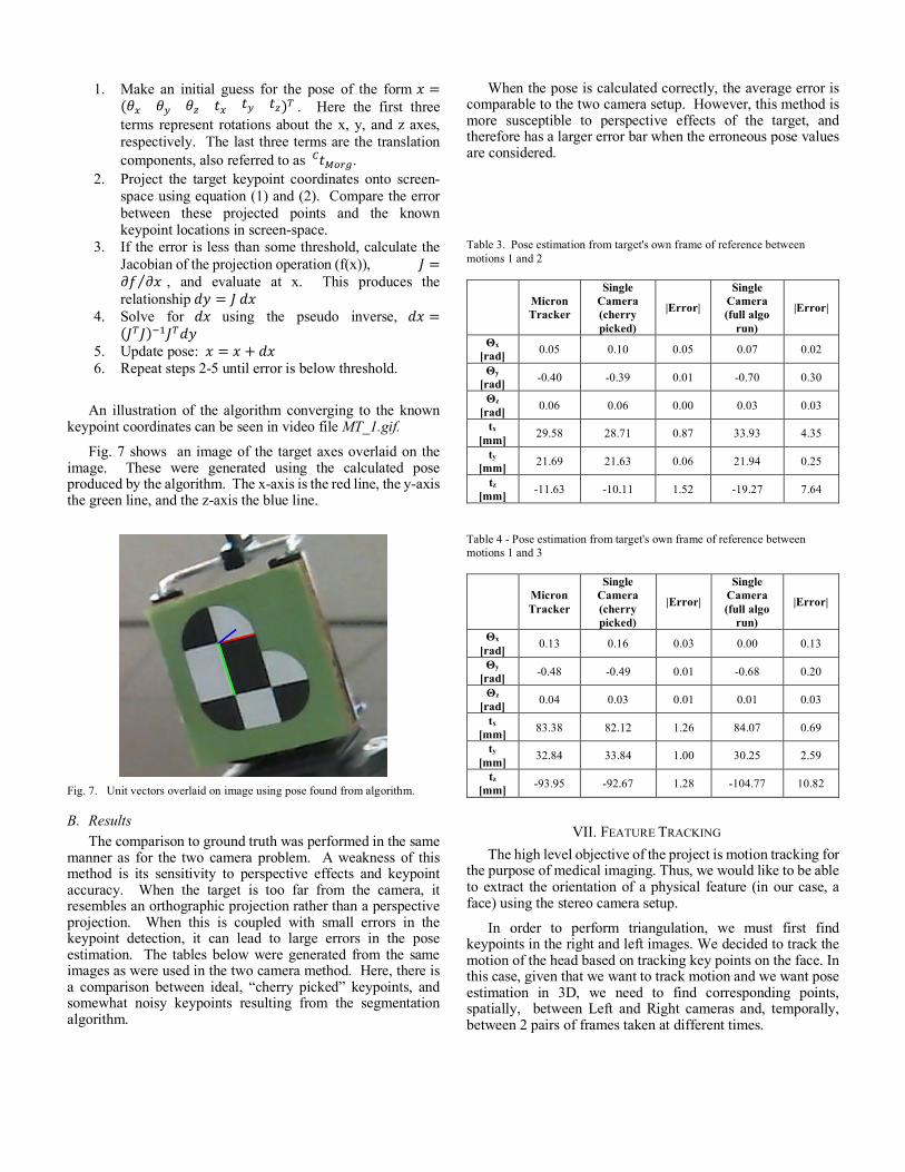
Fig. 7 shows an image of the target axes overlaid on the image. These were generated using the calculated pose produced by the algorithm. The x-axis is the red line, the y-axis the green line, and the z-axis the blue line.

Fig. 7. Unit vectors overlaid on image using pose found from algorithm.

B. Results The comparison to ground truth was performed in the same

manner as for the two camera problem. A weakness of this method is its sensitivity to perspective effects and keypoint accuracy. When the target is too far from the camera, it resembles an orthographic projection rather than a perspective projection. When this is coupled with small errors in the keypoint detection, it can lead to large errors in the pose estimation. The tables below were generated from the same images as were used in the two camera method. Here, there is a comparison between ideal, “cherry picked” keypoints, and somewhat noisy keypoints resulting from the segmentation algorithm.

When the pose is calculated correctly, the average error is comparable to the two camera setup. However, this method is more susceptible to perspective effects of the target, and therefore has a larger error bar when the erroneous pose values are considered.

Table 3. Pose estimation from target's own frame of reference between motions 1 and 2

Micron Tracker

Single Camera (cherry picked)

|Error|

Single Camera (full algo

run)

|Error|

Θx [rad] 0.05 0.10 0.05 0.07 0.02

Θy [rad] -0.40 -0.39 0.01 -0.70 0.30

Θz [rad] 0.06 0.06 0.00 0.03 0.03

tx [mm] 29.58 28.71 0.87 33.93 4.35

ty [mm] 21.69 21.63 0.06 21.94 0.25

tz [mm] -11.63 -10.11 1.52 -19.27 7.64

Table 4 - Pose estimation from target's own frame of reference between motions 1 and 3

Micron Tracker

Single Camera (cherry picked)

|Error|

Single Camera (full algo

run)

|Error|

Θx [rad] 0.13 0.16 0.03 0.00 0.13

Θy [rad] -0.48 -0.49 0.01 -0.68 0.20

Θz [rad] 0.04 0.03 0.01 0.01 0.03

tx [mm] 83.38 82.12 1.26 84.07 0.69

ty [mm] 32.84 33.84 1.00 30.25 2.59

tz [mm] -93.95 -92.67 1.28 -104.77 10.82

VII. FEATURE TRACKING The high level objective of the project is motion tracking for

the purpose of medical imaging. Thus, we would like to be able to extract the orientation of a physical feature (in our case, a face) using the stereo camera setup.

In order to perform triangulation, we must first find keypoints in the right and left images. We decided to track the motion of the head based on tracking key points on the face. In this case, given that we want to track motion and we want pose estimation in 3D, we need to find corresponding points, spatially, between Left and Right cameras and, temporally, between 2 pairs of frames taken at different times.

First, it is necessary to first segment the face from the background. We use the Viola-Jones algorithm in Matlab to detect faces in our images. Using this method we are able to identify complete images of the face, see Error! Reference source not found.. However, we are only able to identify the face in 3 out of 9 pairs of stereo images in our data set. It is possible this algorithm could be improved by improving the quality of the image by removing background noise or changing the lighting conditions We also implemented an algorithm that uses hue detection (CAMShift) [8]. The algorithm was successfully able to detect part or all of the face in an image; however, the bad or partial matches added additional noise to our algorithm.

Fig. 8. Example of the face detection algorithm for pairs of stereo images. The left image illustrates a complete face detection. However, part of the neck is also shown in the image. The right image illustrates a partial face cropping.

We determined point correspondences using the following algorithm that leverages both SIFT descriptors and RANSAC.

Algorithm:

1. Collect 2 pairs of frames with the stereo camera (2x(Left + Right) = 4 images in total)

Perform the following steps on image Frame 1, Left and Right (SIFT + RANSAC): 2. Find keypoints 3. Run Sift Descriptor algorithm on keypoints 4. Generate descriptors vectors for keypoints 5. Find matches between Left and Right Images 6. On Matches found in (4) run RANSAC algorithm to

find the best homography between left and right images

a. For RANSAC, in each iteration 4 points were taken, 30 iterations were ran

b. In each iteration the homography was calculated based on 4 matched points and number of inliers was logged

c. The homography with largest number of inliers was used to remove outliers

7. Filter out all outlier matches and leave only valid matches.

8. Repeat Steps (2) – (8) when images are Frame 1 left, Frame 2 Left

a. Use as keypoints for frame 1 left only the

inlier keypoints that have valid correspondences after RANSAC

9. Repeat Steps (2) – (8) when images are Frame 2 left,

Frame 2 Right a. Use as keypoints for frame 2 left only the

inlier keypoints that have valid correspondences after RANSAC

10. Filter in all 4 images only the keypoints that had valid

correspondences in all 3 aforementioned SIFT + RANSAC steps.

11. Perform triangulation for each frame (based on 2 images and corresponding points)

12. Estimate the pose.

Frame 1 LEFT, Frame 1 Right:

Frame 1 Left, Frame 2 Left:

Frame 2 Left, Frame 2 Right:

Frame 1 Left, Frame 1 Right (After points filtration):

Fig. 9. Example of keypoint detection using our proposed algorithm.

A. Results Table 5. Results of the feature tracking algorithm compared to the magnetic tracker data.

Stereo

Camera Magnetic Tracker

Error

ΔX 30.89 -110 140.89

ΔY 60.89 39 21.81

ΔZ 150.1 36.9 113.2

Results are quite far (> 10 cm), However this can be mostly

explained by poor correspondence between points to triangulate well the 3D point. The inaccuracy of the magnetic tracker collection also contributed to this error.

The drawack of this method is that it requires correspondence in the two directions that requires an accurate and robust manner of describing points between cameras.

VIII. COMPARISONS OF METHODS We compare the three motion tracking methods by

assessing the algorithm accuracy, algorithm speed, and the physical set-up for taking images.

A. Stereo Camera Method: PROS

• Does not require prior knowledge about the tracked target

• Lower computation time (0.67 sec) • Similar calibration Method to single camera

CONS

• Requires accurate correspondence between between points in both cameras

• Requires calibration of both cameras • Sensitive to focus variation between cameras • Computation time would be higher for a better

triangulation method

B. Single Camera Method: PROS

• Comparable accuracy to two camera setup. • Only one camera and a marker.

CONS

• Run-time too long for real-time motion correction (1.5s per frame not including target detection plust time to detect the target).

• Accuracy needs to be improved to sub-millimeter for medical applications.

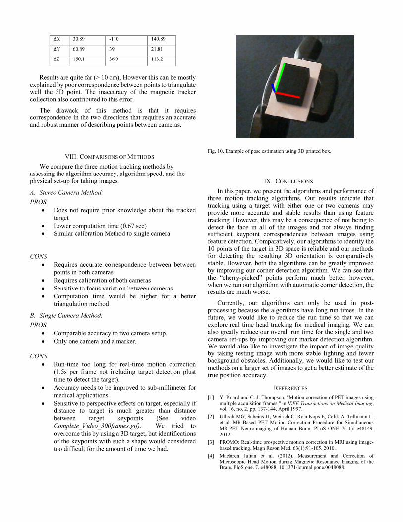
• Sensitive to perspective effects on target, especially if distance to target is much greater than distance between target keypoints (See video Complete_Video_300frames.gif). We tried to overcome this by using a 3D target, but identifications of the keypoints with such a shape would considered too difficult for the amount of time we had.

Fig. 10. Example of pose estimation using 3D printed box.

IX. CONCLUSIONS In this paper, we present the algorithms and performance of

three motion tracking algorithms. Our results indicate that tracking using a target with either one or two cameras may provide more accurate and stable results than using feature tracking. However, this may be a consequence of not being to detect the face in all of the images and not always finding sufficient keypoint correspondences between images using feature detection. Comparatively, our algorithms to identify the 10 points of the target in 3D space is reliable and our methods for detecting the resulting 3D orientation is comparatively stable. However, both the algorithms can be greatly improved by improving our corner detection algorithm. We can see that the “cherry-picked” points perform much better, however, when we run our algorithm with automatic corner detection, the results are much worse.

Currently, our algorithms can only be used in post-processing because the algorithms have long run times. In the future, we would like to reduce the run time so that we can explore real time head tracking for medical imaging. We can also greatly reduce our overall run time for the single and two camera set-ups by improving our marker detection algorithm. We would also like to investigate the impact of image quality by taking testing image with more stable lighting and fewer background obstacles. Additionally, we would like to test our methods on a larger set of images to get a better estimate of the true position accuracy.

REFERENCES [1] Y. Picard and C. J. Thompson, "Motion correction of PET images using

multiple acquisition frames," in IEEE Transactions on Medical Imaging, vol. 16, no. 2, pp. 137-144, April 1997.

[2] Ullisch MG, Scheins JJ, Weirich C, Rota Kops E, Celik A, Tellmann L, et al. MR-Based PET Motion Correction Procedure for Simultaneous MR-PET Neuroimaging of Human Brain. PLoS ONE 7(11): e48149. 2012.

[3] PROMO: Real-time prospective motion correction in MRI using image-based tracking. Magn Reson Med. 63(1):91-105. 2010.

[4] Maclaren Julian et al. (2012). Measurement and Correction of Microscopic Head Motion during Magnetic Resonance Imaging of the Brain. PloS one. 7. e48088. 10.1371/journal.pone.0048088.

[5] Aksoy Murat at al. (2011). Real-Time Optical Motion Correction for Diffusion Tensor Imaging. Magnetic resonance in medicine: official journal of the Society of Magnetic Resonance in Medicine / Society of Magnetic Resonance in Medicine. 66. 366-78. 10.1002/mrm.22787.

[6] Fulton Roger et al. (2002). Errata to "correction for head movements in positron emission tomography using an optical motion-tracking system". Nuclear Science, IEEE Transactions on. 49. 2037- 2038. 10.1109/TNS.2002.805528.

[7] Z. Zhang, "A flexible new technique for camera calibration,“ in IEEE Transactions on Pattern Analysis and Machine Intelligence, 2000

[8] Face Detection and Tracking Using CAMShift. https://www.mathworks.com/help/vision/examples/face-detection-and-tracking-using-camshift.html. 2014.

[9] W. Hoff, “EGGN 512 – Lecture 16-1 Pose Estimation”, 2/22/2012, https://www.youtube.com/watch?v=kq3c6QpcAGc&list=PL4B3F8D4A5CAD8DA3&index=36

[10] R. Sara. The Triangulation Problem. 3D Computer Vision: IV. 10/30/2012. Computing with a Camera Pair (p. 85/213). http://cmp.felk.cvut.cz/cmp/courses/TDV/2012W/lectures/tdv-2012-07-anot.pdf

APPENDIX Jonathan and Tom worked on the keypoint detection and image segmentation code. Tom worked on the single camera detection algorithm. Alex worked on the two camera-detection algorithm. Alex worked on the feature detection algorithm. Sophia implemented face detection algorithm. Sophia collected the calibration images and ground truth data with Jonathan’s help.