Embed Size (px)
Citation preview
MOTION PLANNING WITH LOCALIZATION AND
MAPPING UNCERTAINTIES FOR A MOBILE
MANIPULATOR IN EXPLORATION AND INSPECTION
TASKS
by
Yifeng Huang
B.A.Sc., Tianjin University, P.R.China, 1996
M.A.Sc., China Academic Institute of Science, Shenyang Institute of Automation, 1999
a thesis submitted in partial fulfillment
of the requirements for the degree of
Doctor of Philosophy
in the School of
Engineering Science
c© Yifeng Huang 2009
SIMON FRASER UNIVERSITY
Spring 2009
All rights reserved. This work may not be
reproduced in whole or in part, by photocopy
or other means, without the permission of the author.

Title of thesis: Motion Planning with Localization and Nlapping Uncertain-
ties for a Nlobile Manipulator in Exploration and Inspection
Tasks
Examining Committee: Dr. N{irza Faisal Beg
Chair
Dr. Kamal K. Gupta. Scnior Supervisor
Dr. Ahmad Rad, Supervisor
Dr. Carlo Menon, SFU Examiner
Dr. Thierry Simeon, External Exarniner,
Director Research, LAAS
Toulouse. France
Name:
Degree:
APPROVAL
Yif'eng Huang
Doctor of Philosophy
Date Approved: A'{ '1 "J, z oo'

Last revision: Spring 09
Declaration of Partial Copyright Licence The author, whose copyright is declared on the title page of this work, has granted to Simon Fraser University the right to lend this thesis, project or extended essay to users of the Simon Fraser University Library, and to make partial or single copies only for such users or in response to a request from the library of any other university, or other educational institution, on its own behalf or for one of its users.
The author has further granted permission to Simon Fraser University to keep or make a digital copy for use in its circulating collection (currently available to the public at the “Institutional Repository” link of the SFU Library website <www.lib.sfu.ca> at: <http://ir.lib.sfu.ca/handle/1892/112>) and, without changing the content, to translate the thesis/project or extended essays, if technically possible, to any medium or format for the purpose of preservation of the digital work.
The author has further agreed that permission for multiple copying of this work for scholarly purposes may be granted by either the author or the Dean of Graduate Studies.
It is understood that copying or publication of this work for financial gain shall not be allowed without the author’s written permission.
Permission for public performance, or limited permission for private scholarly use, of any multimedia materials forming part of this work, may have been granted by the author. This information may be found on the separately catalogued multimedia material and in the signed Partial Copyright Licence.
While licensing SFU to permit the above uses, the author retains copyright in the thesis, project or extended essays, including the right to change the work for subsequent purposes, including editing and publishing the work in whole or in part, and licensing other parties, as the author may desire.
The original Partial Copyright Licence attesting to these terms, and signed by this author, may be found in the original bound copy of this work, retained in the Simon Fraser University Archive.
Simon Fraser University Library Burnaby, BC, Canada

Abstract
In this research, we address the motion planning (MP) problem in real world robotic ex-
ploration and inspection tasks, where robot localization and mapping uncertainties have to
be incorporated into the planned motions. The robot considered in this work is a mobile
manipulator system, which combines the mobility of the base with the dexterousness of
the manipulator, and therefore is suitable for the exploration and inspection task in both
open spaces and locally cluttered environments. To explore the environment, a laser range
scanner is mounted in the front of the mobile base.
The first part of this work considers localization and mapping uncertainties in the mo-
tion planning problem. We propose RRT-SLAM, which uses a rapidly-exploring random
tree (RRT) in conjunction with a simulated particle based simultaneous localization and
mapping (SLAM) algorithm to expand the tree. The simulated SLAM explicitly accounts
for localization and mapping uncertainties in the planning stage. Moreover, the RRT itself
is represented in the uncertainty-configuration space (UC-space), which is an augmented
configuration space with an extra dimension of uncertainty. The collision probability along
a planned path is explicitly calculated and is used to select a planned path. Since the
standard Euclidean metric does not reflect the structure of the UC-space well, we address
the efficiency of the RRT in the UC-space. We treat the issue from a data clustering point
of view and propose a fractal dimension (FD) based checking criterion for efficient node
generation. The advantages of our FD based approach are illustrated and discussed, and
we demonstrate the positive results in simulations.
The second part of this research addresses planning motions for the manipulator to
accomplish an inspection task, with the base staying stationary. Therefore, no sensor ob-
servation is available during the motion. We extend the probabilistic roadmap (PRM)
algorithm to plan motions. Since the base pose of the manipulator is not precisely known
iii

due to the localization uncertainty, the path query of the roadmap becomes a constrained
shortest path problem, and is fundamentally different from the query in the standard PRM.
We prove that this path query is an NP-hard problem, and propose an lazy path query
algorithm that judiciously combines a k-shortest path algorithm with a labeling algorithm.
The algorithm rules out large classes of paths, hence leading to efficiency.
The RRT-SLAM is tested on an actual PowerBot and the experimental results show the
effectiveness and benefits of our integrated approach. We also implemented and tested our
integrated planner for the mobile manipulator in simulations. The simulated system is a
mobile base with a 3-dof manipulator mounted on it. A Hokuyo laser range sensor, mounted
on the mobile base, is also simulated. The effectiveness of the combined integrated planner
is demonstrated via these simulations.
iv

To my wife
v

Acknowledgments
I would like to thank the following people for contribution of this thesis. With the support
of individuals below, I went through some of the best years in my life.
I would like to first express my appreciation to my supervisor, Dr. Kamal K. Gupta, for
his guidance and support. I can not convey how thankful I am to him.
I would also like to thank my examining committee, Dr. Ahmad Rad, Dr. Carlo Menon
and Dr. Thierry Simeon for their extremely valuable suggestions.
Special thanks to my lab-mates, Lila Torabi, Moslem Kazemi, Zhengwang Yao and Yi
Li, for their comments and support.
My sincere appreciation also goes to the brothers and sisters in SFU Fellowship. Thanks
for their company with me and my family, and from their sharing and testimonies, I acquired
the true treasure of life.
Last, I like to thank my family for their encouragements, support and patience.
vi

Contents
Approval ii
Abstract iii
Dedication v
Acknowledgments vi
Contents vii
List of Tables xi
List of Figures xii
Notation xvi
Publications xx
Acronyms xxi
1 Introduction 1
1.1 Introduction . . . . . . . . . . . . . . . . . . . . . . . . . . . . . . . . . . . . . 1
1.2 Overview of the Problem and Our Algorithms . . . . . . . . . . . . . . . . . . 7
1.2.1 RRT-SLAM: a Motion Planner with Localization and Mapping Un-
certainties . . . . . . . . . . . . . . . . . . . . . . . . . . . . . . . . . . 8
1.2.2 Lazy-PRM-BU: a Motion Planner for a Manipulator with Base Pose
Uncertainty . . . . . . . . . . . . . . . . . . . . . . . . . . . . . . . . . 10
vii

1.2.3 Delaunay Triangulation Inspired Adaptive k Nearest Neighbor Sample
Connection Strategy for PRM . . . . . . . . . . . . . . . . . . . . . . . 11
1.3 Related Work . . . . . . . . . . . . . . . . . . . . . . . . . . . . . . . . . . . . 11
1.3.1 Model-Based Motion Planning . . . . . . . . . . . . . . . . . . . . . . 11
1.3.2 Motion Planning Under Control and Sensing Uncertainties in Known
Environments . . . . . . . . . . . . . . . . . . . . . . . . . . . . . . . . 14
1.3.3 Motion Planning Under Map Uncertainty . . . . . . . . . . . . . . . . 18
1.3.4 Exploring Unknown Environments Under Control and Sensing Uncer-
tainties . . . . . . . . . . . . . . . . . . . . . . . . . . . . . . . . . . . 18
1.3.5 RRT-SLAM Contribution to Current Path Planning Techniques . . . 20
1.3.6 Representations of Localization and Mapping Uncertainties . . . . . . 21
1.3.7 Representations of Physical Space . . . . . . . . . . . . . . . . . . . . 21
1.3.8 Constrained Shortest Path problem (CSPP) and Lazy Path Query of
the Roadmap . . . . . . . . . . . . . . . . . . . . . . . . . . . . . . . . 22
1.4 Publication Notes . . . . . . . . . . . . . . . . . . . . . . . . . . . . . . . . . . 22
1.5 Thesis Contributions . . . . . . . . . . . . . . . . . . . . . . . . . . . . . . . . 23
1.6 Thesis Outline . . . . . . . . . . . . . . . . . . . . . . . . . . . . . . . . . . . 24
2 RRT-SLAM 25
2.1 FastSLAM: an Overview . . . . . . . . . . . . . . . . . . . . . . . . . . . . . . 25
2.2 Simulated SLAM Framework: Determining Collision Probability Along a
Planned Path . . . . . . . . . . . . . . . . . . . . . . . . . . . . . . . . . . . . 27
2.2.1 Simulated SLAM Framework . . . . . . . . . . . . . . . . . . . . . . . 27
2.2.2 Particle Based Simulated Localization . . . . . . . . . . . . . . . . . . 32
2.3 Planning Motion with Localization and Mapping Uncertainties (RRT-SLAM) 39
2.4 Simulations . . . . . . . . . . . . . . . . . . . . . . . . . . . . . . . . . . . . . 44
2.5 Experiments . . . . . . . . . . . . . . . . . . . . . . . . . . . . . . . . . . . . . 46
2.6 Parameter Values Related to RRT-SLAM . . . . . . . . . . . . . . . . . . . . 48
2.7 Discussion . . . . . . . . . . . . . . . . . . . . . . . . . . . . . . . . . . . . . . 49
3 RRT-SLAM-FD 50
3.1 Tree Exploration in the Uncertainty-Configuration Space (UC-Space) . . . . . 50
3.1.1 Classic RRT’s Dependence on Metrics . . . . . . . . . . . . . . . . . . 51
3.1.2 RRT-Blossom . . . . . . . . . . . . . . . . . . . . . . . . . . . . . . . . 52
viii

3.1.3 Original Regression Condition in the UC-Space . . . . . . . . . . . . . 53
3.2 Outlier Detection Mediated Regression Checking . . . . . . . . . . . . . . . . 57
3.2.1 Fractal Dimension . . . . . . . . . . . . . . . . . . . . . . . . . . . . . 57
3.2.2 Applying FD as a Regression Condition . . . . . . . . . . . . . . . . . 58
3.3 Improving RRT-SLAM Efficiency in the UC-Space: RRT-SLAM-FD . . . . . 58
3.3.1 Discussions on RRT-SLAM-FD . . . . . . . . . . . . . . . . . . . . . . 62
3.3.2 Box Counting: an Algorithm to Determine FD . . . . . . . . . . . . . 63
3.4 Simulations . . . . . . . . . . . . . . . . . . . . . . . . . . . . . . . . . . . . . 64
4 Lazy-PRM-BU 69
4.1 Problem Formulation . . . . . . . . . . . . . . . . . . . . . . . . . . . . . . . . 69
4.1.1 Underlying Structure of PRM with Base Pose Uncertainty . . . . . . . 71
4.1.2 CP-CSPP: an NP-hard Problem . . . . . . . . . . . . . . . . . . . . . 73
4.1.3 Using the Labeling Algorithm to Solve CP-CSPP . . . . . . . . . . . . 75
4.2 Lazy-PRM with Base Pose Uncertainty . . . . . . . . . . . . . . . . . . . . . 77
4.2.1 Lazy-PRM Review . . . . . . . . . . . . . . . . . . . . . . . . . . . . . 77
4.2.2 Lazy-PRM with Base Uncertainty . . . . . . . . . . . . . . . . . . . . 77
4.2.3 The k-shortest Path Algorithm . . . . . . . . . . . . . . . . . . . . . . 78
4.2.4 Calculating the Shortest Path in an Equivalent Class . . . . . . . . . . 80
4.2.5 Lazy-PRM-BU . . . . . . . . . . . . . . . . . . . . . . . . . . . . . . . 81
4.2.6 Roadmap Construction and Node Enhancement . . . . . . . . . . . . 83
4.2.7 Detecting an N-edge . . . . . . . . . . . . . . . . . . . . . . . . . . . . 84
4.2.8 Path Verification from Both Directions . . . . . . . . . . . . . . . . . . 84
4.3 Simulations . . . . . . . . . . . . . . . . . . . . . . . . . . . . . . . . . . . . . 84
4.4 A Motion Planner for the Mobile Manipulator System in an Inspection Task 90
5 DTC 93
5.1 Delaunay Triangulation Review . . . . . . . . . . . . . . . . . . . . . . . . . . 93
5.2 PRM Sample Connection Strategy Review . . . . . . . . . . . . . . . . . . . . 94
5.3 Delaunay Triangulation Inspired Connection (DTC) Strategy . . . . . . . . . 95
5.3.1 Constructing a Delaunay Triangulation Neighborhood . . . . . . . . . 96
5.3.2 Delaunay Triangulation Inspired Adaptive Roadmap Connection (DTC)100
5.3.3 Node Enhancement . . . . . . . . . . . . . . . . . . . . . . . . . . . . . 102
5.4 Simulations . . . . . . . . . . . . . . . . . . . . . . . . . . . . . . . . . . . . . 103
ix

6 Conclusions and Future work 106
6.1 Future Work . . . . . . . . . . . . . . . . . . . . . . . . . . . . . . . . . . . . 107
Appendix 109
A System Implementation 109
A.1 The Simulated Mobile Manipulator Test-bed System . . . . . . . . . . . . . . 109
A.1.1 The Mobile Manipulator Simulator . . . . . . . . . . . . . . . . . . . . 109
A.1.2 Robot System Software Implementation and Architecture . . . . . . . 110
A.2 Sonar-Based Local Collision Avoidance for the Mobile Base During Path Ex-
ecution . . . . . . . . . . . . . . . . . . . . . . . . . . . . . . . . . . . . . . . . 115
Bibliography 117
x

List of Tables
1.1 RRT-SLAM’s relationship with current existing path planning techniques
considering localization and/or mapping uncertainties. . . . . . . . . . . . . . 20
2.1 Parameter values applied in RRT-SLAM for the simulations and experiments.
Unless specified otherwise, all simulations and experiments used these values. 49
3.1 Simulation results for Problems A, B and C. . . . . . . . . . . . . . . . . . . . 68
4.1 Results for Lazy-PRM-BU with pruning invalid equivalent classes. . . . . . . 87
4.2 Results for PRM-BU. . . . . . . . . . . . . . . . . . . . . . . . . . . . . . . . 87
4.3 Number of collision checking for Lazy-PRM-BU and PRM-BU. . . . . . . . . 87
4.4 Results for Lazy-PRM-BU without pruning invalid equivalent classes. . . . . 89
4.5 The number of failure times (FT) and worst case time (WT) for Lazy-PRM-
BU (30 runs) with (w. pr.) and without (w.t. pr.) pruning invalid equivalent
classes. Time limit is 1000 and 1500 seconds for SMALL and LARGE uncer-
tainty, respectively. . . . . . . . . . . . . . . . . . . . . . . . . . . . . . . . . . 89
5.1 Simulation results for problems A, B, C, D and E. . . . . . . . . . . . . . . . 105
A.1 VFH parameters applied. . . . . . . . . . . . . . . . . . . . . . . . . . . . . . 116
xi
List of Figures
1.1 The SFU mobile manipulator system (with an enlarged picture of the Hokuyo
URG-04LX range scanner) in the RAMP laboratory at Simon Fraser University. 2
1.2 The overall exploration/inspection process consists of mainly three stages. . . 3
1.3 Two paths planned with different localization uncertainties considered. White
areas represent free space. Gray areas represent unknown areas, which are
treated as obstacles (in black color) as well. The ellipses along the path
represent the localization uncertainty along the path. The sensing range is
4m, and the grid size in the map is 1m. . . . . . . . . . . . . . . . . . . . . . 5
1.4 The simulated test-bed for the motion planner under robot localization and
mapping uncertainties. The mobile base is a simulated PowerBot of size 80cm
by 65cm. A simulated Hokuyo laser range finder is mounted in the front of
the mobile base. The manipulator has 3 links. The black areas are obstacles,
but unknown to the robot at beginning. Area covered by the scan of the
range finder is gray, and becomes known to the robot. The gray rays are
simulated sonar beams. . . . . . . . . . . . . . . . . . . . . . . . . . . . . . . 6
1.5 Robot motion planning in a wide open area. The ellipses along the two paths
represent the localization uncertainties. . . . . . . . . . . . . . . . . . . . . . 19
2.1 Sample trail particles from the state particle sets (L0, L1, ..., L4) at each
time instant (t=0 to 4). The number of trail particles in the trail particle set
is set as 4, which equals the number of state particles at each time instant. . 34
2.2 Sample trail particles sequentially over each time instant. . . . . . . . . . . . 36
2.3 A typical random tree returned by Algorithm-5 . . . . . . . . . . . . . . . . . 43
xii

2.4 The same goal but different goal uncertainties were given to the robot. The
paths found were different. For the low uncertainty case (b), robot prefers to
go closer to known obstacles to localize itself better. . . . . . . . . . . . . . . 44
2.5 Comparing solution paths returned by RRT-SLAM and the classic RRT in
the simulated environment. . . . . . . . . . . . . . . . . . . . . . . . . . . . . 46
2.6 A map of the RAMP lab in the Applied Science Building at SFU. The next
goal of the robot is marked. . . . . . . . . . . . . . . . . . . . . . . . . . . . . 47
2.7 Comparing solution paths returned by RRT-SLAM and the standard RRT in
the RAMP lab environment shown in Figure 2.6. . . . . . . . . . . . . . . . . 47
2.8 Trace of the mobile base as it executes the path planned using RRT-SLAM
for the RAMP lab environment. . . . . . . . . . . . . . . . . . . . . . . . . . . 48
3.1 The regression checking mechanism for RRT-Blossom. . . . . . . . . . . . . . 53
3.2 Failure of the original regression condition in the UC-space. . . . . . . . . . . 54
3.3 The live tree nodes picked by the regression condition (Equation 3.1) intro-
duced in RRT-blossom. . . . . . . . . . . . . . . . . . . . . . . . . . . . . . . 55
3.4 Distribution of the live nodes (dark) under the original regression condition.
The dormant nodes are shown in light color. . . . . . . . . . . . . . . . . . . . 56
3.5 An example of applying the original regression checking condition (Equation
3.1) in the UC-space. Only live nodes are shown. A small number of live
nodes (dark colored) are available for further extensions. Nodes in gray color
are also live nodes, but they have been extended more than 8 times and hence
will not be further extended (refer to the explanation for RRT-Blossom). . . 57
3.6 The live tree nodes picked by the new FD based regression condition (Equa-
tion 3.3). . . . . . . . . . . . . . . . . . . . . . . . . . . . . . . . . . . . . . . 62
3.7 Distribution of the live nodes under the new FD based regression condition. . 62
3.8 FD values for the data set of the RRT-SLAM nodes, with the initial data set
in the UC-space, for 5 runs. . . . . . . . . . . . . . . . . . . . . . . . . . . . . 64
3.9 Problems A and B. . . . . . . . . . . . . . . . . . . . . . . . . . . . . . . . . . 65
3.10 Problem C. . . . . . . . . . . . . . . . . . . . . . . . . . . . . . . . . . . . . . 65
xiii
3.11 Tree structures in the UC-space, shown in 2D view ((a1), (b1) and (c1))
and 3D view (the rests), acquired by applying RRT-SLAM ((a1) and (a2)),
RRT-SLAM-Blossom ((b1), (b2) and (b3)) and RRT-SLAM-FD ((c1), (c2)
and (c3)), for Problem C. For RRT-SLAM-Blossom and RRT-SLAM-FD,
the nodes (branches) in black and gray color are the live and dormant nodes,
respectively. In (b3) and (c3), only live nodes are shown. . . . . . . . . . . . . 67
4.1 For a manipulator path, there are correspondingly N possible sequences of
configurations swept by the whole mobile manipulator. . . . . . . . . . . . . . 70
4.2 Roadmap G in Cm, and the corresponding graph set G = {G[1], G[2], G[3]}constructed in Cbm (N = 3). . . . . . . . . . . . . . . . . . . . . . . . . . . . . 72
4.3 A graph G constructed to transform the PARTITION problem into CP-CSPP 74
4.4 Building of the branching structure of the shortest path tree T3. . . . . . . . . 80
4.5 Four different start/goal problems. Left: paths planned with PRM-BU with
base uncertainty (LARGE). Right: paths planned with classic PRM with no
uncertainty taken into account and with the base pose at the most weighted
particle. . . . . . . . . . . . . . . . . . . . . . . . . . . . . . . . . . . . . . . . 86
4.6 Running time for problems A to D for all the 30 runs. . . . . . . . . . . . . . 88
4.7 The robot is given an end effector position as goal shown in sub-figure (a),
which is a partially explored environment. The end effector position is marked
by the black square. In (b), the mobile base first moves close to the designated
end effector position (path planned with RRT-SLAM), and then execute the
manipulator path returned by the Lazy-PRM-BU, with the base being sta-
tionary (c). . . . . . . . . . . . . . . . . . . . . . . . . . . . . . . . . . . . . . 92
5.1 Delaunay triangulation and Voronoi diagram of a 2D points set. Square dots
are the points in the point set. Light gray polygon regions are the Voronoi
cells and dark triangles form the Delaunay triangulation. . . . . . . . . . . . . 95
5.2 Delaunay triangulation inherently uses both distance and direction informa-
tion. See text for explanation. . . . . . . . . . . . . . . . . . . . . . . . . . . . 96
5.3 Probability for a node of ranking ki to be DN of node nc, in 6-dimensional
space . . . . . . . . . . . . . . . . . . . . . . . . . . . . . . . . . . . . . . . . . 98
5.4 Selection of kb for each dimension from 2 to 10 . . . . . . . . . . . . . . . . . 99
xiv

5.5 Relationship between the number of uniform nodes and radius selection (the
average value) in 2, 4 and 6-dimensional spaces. . . . . . . . . . . . . . . . . . 101
5.6 Problems A (left) and B (right) – 2D rigid mobile robot . . . . . . . . . . . . 103
5.7 Problems C (left) and D (right) – 4-link planar manipulator with fixed base. . 104
5.8 Problem E – 6-link planar manipulator with fixed base. . . . . . . . . . . . . 104
A.1 Modified MobileSim to support the control of an on-board manipulator.
Shaded areas indicate our modifications to the original MobileSim. . . . . . . 110
A.2 System software for the mobile base that consists of mainly three threads:
the user interface, the planner, and the ARIA path execution module. . . . . 111
A.3 The user interface consists of three windows (marked as A, B and C). Window
A and B are for displaying information and results, and Window C is for user
inputs. See the text for detailed explanation. For local sonar map with robot
at the center (right-bottom corner of window A), please refer to Section A.2
for detailed explanation about this area. . . . . . . . . . . . . . . . . . . . . . 114
xv

Notation
π a path, consisting of a sequence of robot configurations.
νπ a trail that is traversed by robot when it follows π.
t time index.
κπ potential sequence of sensor observations, when robot follows π.
κν the sequence of sensor observations along ν.
qsubscript a configuration or robot state indicated by the subscript.
m an environment model.
♯S the number of SLAM particles.
♯L the number of localization particles.
V a binary random variable indicates the event that robot trail ν is
collision-free (1) or not (0).
Π a binary random variable indicates the event that robot is collision-free
(1) or not (0), when it follows π.
ν [i] the ith trail particle.
m[i] the environment model associated with the ith SLAM particle.
κ[i] the sequence of sensor observations in the jth simulated sequence.
aπt when following π, the control command applied to the robot at time t.
qnext the next intermediate goal when following a path.
q∗t robot configuration corresponding to the most weighted particle in a
particle set.
M the number of repeated sequences of simulated SLAM (or localization)
along a path.
xvi

ν [i,j] the ith trail particles, which are acquired at the jth sequence of simulated
SLAM (or localization).
m[i,j] the environment model associated with the ith SLAM particles, which
are acquired in the jth sequence of simulated SLAM.
m∗ the map associated with the most weighted SLAM particle before plan-
ning the motion.
m∗b the binarized version of m∗.
ν [i]f the ith trail particle that is collision-free in map m∗b .
Y a set of SLAM particles.
Lt the set of particles that represents qt.
L′
t+1 the set of particles that represents the initial guess of robot state at
t + 1.
[x, y, θ] a pose (position x, y and orientation θ ) for the mobile base.
|A| size of area covered by the range sensor.
κ∗t the sequence of sensor observations received from 0 to t in one simulated
sequence.
Bugoalthreshold for the localization uncertainty at goal position.
Bu threshold for the localization uncertainty for a RRT-SLAM tree node.
Pthresh a threshold between [0, 1]. The probability of the solution path being
collision-free has to be higher than τf .
φt−1 the number of particles in Lt−1 , who have decedents in Lt.
ηt−1 ηt−1 = φt−1
♯L.
τp a threshold between [0, 1]. In case ηt−1 ≤ τp, we assume qt−1 is inde-
pendent of qt.
ω[i] the weight of the ith particle in a particles set.
ω[i] the weight of the ith trail particle in a particles set.
n a graph/tree node.
qn the configuration at graph node n.
Tt a data set that stores trail particle set information at time t.
Tnia data set that stores trail particle set information at graph node ni.
xvii

ν[i]ft+1
at time t + 1, the weight of the ith trail particle that is collision-free.
Pni
free the probability that robot is collision-free when arriving graph node ni.
ϕ a weight between [0, 1].
ρ(.) a distance measurement.
DQ the fractal dimension of a data set.
di a grid.
pi the frequency of the data points falling into the cell di.
r the size of a grid.
Nr the number of grids occupied by the data set for a given grid size gr.
fthresh the threshold for a reasonable change of fractal dimension.
fstep the adjustment step of fthresh.
△f the change of fractal dimension before and after a data point is added
into the data set.
Ti the shortest path tree structure constructed from the i shortest paths.
B(nu) a bundle of shortest paths corresponding to tree node nu in Ti.
Bi the set of first i shortest paths in G.
B the set of all the paths in G.
Bi complement of Bi, Bi = B\Bi.
C(nu) a class of paths in Bi corresponding to tree node nu of Ti.
C(nu, nv) a class of paths in Bi corresponding to a tree branch (nu, nv) of Ti.
G a roadmap graph for the manipulator.
G a set of graphs.
Gi the ith graph in G.
C(π) the length (cost) of the path π.
C the configuration space.
Cm the manipulator’s configuration space.
Cmb the mobile manipulator’s configuration space.
e a graph/tree edge/brach.
Πe a binary random variable indicating the event that robot is collision-free
(1) or not (0), when it follows a graph edge e.
xviii

nr a random generated node.
nc a tree node that is the nearest to nr, among all the tree nodes.
nnew a new tree node.
π[i] a manipulator path with base pose at the ith particle.
c[i] a binary variable indicating π[i] is free (1) or not (0).
e[na,nb] an edge between two neighbor graph nodes na and nb in G.
V the set of nodes in G.
E the set of edges in G.
πki the kth path reaching to graph node ni in G.
G[i] a roadmap graph for the manipulator, given the base pose is the ith
particle.
n[i]j the jth node of G[i].
e[i] an edge of G[i].
e[i][nj ,nk] an edge of G[i], connecting node n
[i]j and n
[i]k .
Cki accumulated cost (the length) of the πk
i .
P ki the probability of manipulator path πk
i being collision free.
S a data set.
s a data point in S.
V (s) Voronoi region of s.
P a problem.
xix

Publications
1. Y. Huang and K. Gupta. A Delaunay triangulation based node con-
nection strategy for probabilistic roadmap planners. In Proceedings of
IEEE International Conference on Robotics and Automation (ICRA04),
pages 908 - 913, 2004
2. Y. Huang and K. Gupta. An daptive configuration-space and
work-space based criterion for view planning. In Proceedings of
IEEE/RSJ/GI International Conference on Intelligent Robots and Sys-
tems (IROS05), pages 3366- 3371, 2005
3. Y. Huang and K. Gupta. RRT-SLAM for motion planning with mo-
tion and map uncertainty for robot exploration. In Proceedings of
IEEE/RSJ/GI International Conference on Intelligent Robots and Sys-
tems (IROS08), pages 1077-1082, 2008
4. Y. Huang and K. Gupta. Lazy-PRM for a Manipulator with Base Pose
Uncertainty. Submitted to IEEE/RSJ/GI International Conference on
Intelligent Robots and Systems (IROS09), 2009.
xx

Acronyms
ACA Ariadne’s Clew Algorithm
CSPP Constrained Shortest Path Problem
CP-CSPP Collision Probability Constrained Shortest Path Problem
DN Delaunay Neighbor
DOF Degree Of Freedom
DT Delaunay Triangulation
DTC Delaunay Triangulation inspired sample Connection technique
DW Dynamic Window
FD Fractal Dimension
Lazy-PRM PRM with Lazy query technique
Lazy-PRM-BU Lazy-PRM for manipulator with Base pose Uncertainty
LIDAR Light Detection And Ranging
LP Linear Programming
MDP Markov Decision Process
MP Motion Planning
MPK Motion Planning Kernel
NNC Nearest Neighbor Connection strategy
POMDP Partially Observable Markov Decision Process
PRM Probabilistic Roadmap Method
PRM-BU PRM for manipulator with Base pose Uncertainty
RAMP Robotic Algorithms and Motion Planning Laboratory
RRT Rapid-exploring Random Tree
RRT-Blossom RRT with regression checking technique
xxi

RRT-CT RRT with Collision Tendency technique
RRT-SLAM-
Blossom
RRT-SLAM with original regression checking technique in RRT-
Blossom
RRT-SLAM-FD RRT-SLAM with FD based regression checking technique
RRT-SLAM RRT in conjunction with SLAM technique
SFU Simon Fraser University
SLAM Simultaneously Localization And Mapping
VFH Vector Field Histogram
WCSPP Weight Constrained Shortest Path Problem
xxii

Chapter 1
Introduction
1.1 Introduction
Robot platforms that mix mobility and manipulation, such as humanoid robots or mobile
manipulators, have recently gained more attention. In the long run, expectations are that
these systems will be capable of substituting human beings in many challenging tasks, e.g.,
exploration/inspection in unknown environments [1], samples collection in hazard areas [2],
cargo picking up and transportation [3], and daily service [4].
This research is a step towards the long term goal of the Robotic Algorithms and Motion
Planning (RAMP) laboratory at Simon Fraser University, to build a fully autonomous mobile
manipulator system that is capable of carrying out exploration, inspection and manipulation
tasks in unknown environments. Building such a system requires integrating a variety of
robotic disciplines including, for example, path planning [5, 6], sensing and modeling [7],
vision [8], target tracking [9], and robot control [10].
The mobile manipulator system (Figure 1.1) in RAMP includes a PowerBotTM
mobile
base (with a weight of 120kg and a payload of up to 100kg), and a SchunkTM manipulator,
consisting of a 6-link arm, mounted on the top of the base. The base is heavy enough, so we
can assume that the manipulator motion is precise w.r.t. the base frame when the base is
kept still. The PowerBot can be considered as a holonomic mobile base since it has a very
small turning radius. A Hokuyo URG-04LX range scanner (based on Light Detection and
Ranging (LIDAR) technology), having a sensing range of 4.0m and a span angle of 180◦,
is fixed on the mobile robot and points to the front. Fourteen forward and fourteen rear
sonar sense obstacles from 15cm to 7m. At the end effector of the manipulator, one could
1

CHAPTER 1. INTRODUCTION 2
attach an “eye” sensor, (e.g., a camera or a range finder) for inspection or object modeling
tasks [11, 12, 13], and/or a gripper for visual based [9] grasping/manipulation tasks. Such a
specific system setup combines the mobility of the base with the manipulation ability of the
arm, and therefore is suitable for the exploration/inspection task in both open spaces (by
using the range scanner at base) [7] and cluttered environments (by using the eye sensor)
[14].
Figure 1.1: The SFU mobile manipulator system (with an enlarged picture of the HokuyoURG-04LX range scanner) in the RAMP laboratory at Simon Fraser University.
The particular application that motivates this research is planning motions for au-
tonomous exploration/inspection in unknown environments. As shown in Figure 1.2, the
whole exploration/inspection process is a plan-move and sense-update loop [11], which con-
sists of mainly three stages in each iteration: I) plan for robot’s next (reachable) configura-
tion, i.e., a view point, to further explore/inspect its environment; II) execute the plan, i.e.,
move to the planned configuration (and sense if further information about the environment

CHAPTER 1. INTRODUCTION 3
is available during the motion); and III) update the robot’s own position and/or the envi-
ronment model. Two subproblems are involved in stage I, the planning stage: I-a) where
to go, also called the next best view (NBV) [11, 12, 15, 16]; and I-b) how to get there, i.e.,
determine a reachable path to get to the next viewpoint. If a final goal is to be reached, it
can be easily incorporated in the overall process.
location and environment
model
Update the robot
Motion Planning
View Planning
Execute the plan
stage
Planning
Start
Figure 1.2: The overall exploration/inspection process consists of mainly three stages.
In this exploration/inspection task, a key sub-task for the robot is to plan its motion to
the next viewpoint without colliding with obstacles (the third block in Figure 1.2). This is
critical for safety of both the robot and the working environment, and is the domain of the
classic motion planning sub-field in robotics.
The very basic motion planning (MP) problem, in a narrow sense, is searching for a path
that can guide the robot from a start place to a goal place without colliding with obstacles.
It assumes that 1) the robot can be precisely controlled, and 2) the environment is also
perfectly known [5]. This type of motion planning problem is also referred to as the model-
based MP. A classic solution to the model-based MP is to search in the configuration space
(C-space, denoted as C) [17], which is the space of possible positions that a robot system
may attain. For example, the C-space of a single point robot moving in ordinary Euclidean

CHAPTER 1. INTRODUCTION 4
3D space is just R3, and the C-space of a open-loop manipulator is the joint space, where
each dimension is the value of one manipulator joint. Then the solution of the model-based
MP is a one-dimensional “path” in the free part of the C-space (denoted as Cfree).
The two assumptions mentioned above, however, are not realistic in many real world
scenarios. For example, the robot may have to explore and construct the environment
model (map) step by step, while moving around, with the collected information about the
environment from on-board sensors. In such a case, robot’s next motion is usually planned
within the known part of the environment, with the unknown part treated as obstacle [14].
However, if the robot control is not precise and the on-board sensors are not noise free, the
robot can not precisely know its own true location (the localization uncertainty), where the
sensor data is collected, which is crucial to environment modeling (i.e., mapping). Therefore,
the constructed environment model usually contains errors and is not precise (the mapping
uncertainty). Locating the true position of the robot (i.e., localization), on the other hand,
requires a precise map. Simultaneously localization and mapping (SLAM) [7], a key advance
in the mobile robotics literature in past decade, attempts to solve this problem, and returns
the best estimation of both the map and the robot position at the same time in the execution
stage.
In this work, we widely use the terms of localization and mapping uncertainty. These
uncertainties are a result of underlying uncertainties in control/motion and in sensing. The
localization uncertainty arises when robot can not perfectly localize itself due to underlying
errors in control/motion and in sensing. The mapping uncertainty aries when the robot
can not build a perfect map due to the control and/or sensing uncertainties [7]. Here, the
control/motion uncertainty arises when the robot execution mechanism can not precisely
execute a control command (for example, due to a slip of the wheel friction or due to the
robot internal design limitation [5]). The sensing uncertainty arises when the sensor can not
supply perfect information about the robot current location (e.g., the on-board odometry
sensors and other range sensors such as laser/sonar sensors are usually not perfect [7]).
We study how to plan robot motions that incorporate the robot localization and mapping
uncertainties. Our motion plan, similar to the classic model-based MP, is a path that consists
of a sequence of robot configurations. However, in the presence of uncertainties, both the
map and the exact robot trajectory along the path in the execution stage are not exactly
known at the planning stage.
Figure 1.3 illustrates an example how path planning is impacted by, e.g., the localization

CHAPTER 1. INTRODUCTION 5
(a) path1 (b) path2
Figure 1.3: Two paths planned with different localization uncertainties considered. Whiteareas represent free space. Gray areas represent unknown areas, which are treated as obsta-cles (in black color) as well. The ellipses along the path represent the localization uncertaintyalong the path. The sensing range is 4m, and the grid size in the map is 1m.
uncertainty, for a mobile base. Note that, in the two sub-figures, both paths are feasible
if the control and sensing are both perfect. However, with the localization uncertainty
considered, a safe motion may require the robot to well localize itself with the on-board
sensor, by staying close to the obstacle, as shown in the Figure 1.3 (a). In Figure 1.3 (b) the
uncertainty along the path increases quickly, because the robot is away from the obstacle
and can not well localize itself, leading to a higher chance of collision.
We use a probabilistic framework in the planning process itself, i.e., a planned path
corresponds to a set of possible executed trails, each with a probability attached to it. This
probabilistic approach is fundamentally different from the standard model-based MP, where
a planned path corresponds to a sequence of configurations.
With the probabilistic framework, the collision status of following a path is associated
with a collision probability. This is also different from the model-based MP, where the
collision status of a solution path is binary as either collision-free or in-collision [5]. We use
this collision probability as a travel cost, and refer to a path as “feasible” if its associated
probability of collision-free is higher than a user defined threshold.
Calculating/evaluating possible hazardous consequences of a path in terms of the col-
lision probability, and efficiently returning a robust solution path are contributions of this
thesis.

CHAPTER 1. INTRODUCTION 6
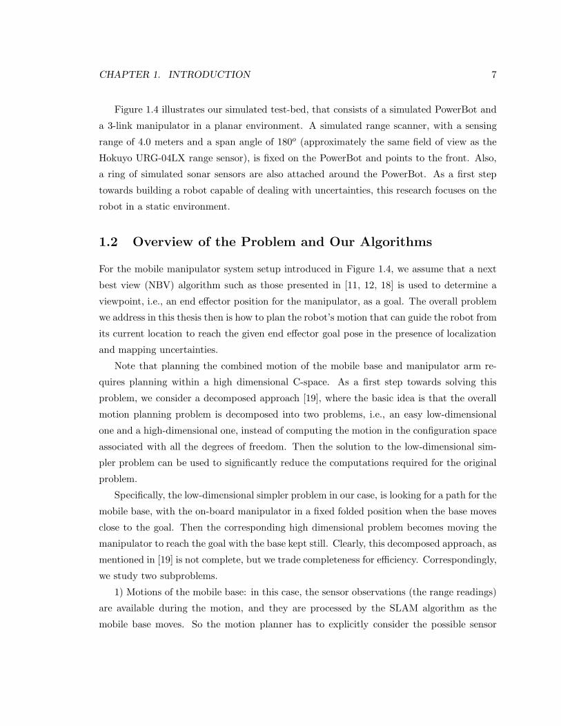
Figure 1.4: The simulated test-bed for the motion planner under robot localization andmapping uncertainties. The mobile base is a simulated PowerBot of size 80cm by 65cm.A simulated Hokuyo laser range finder is mounted in the front of the mobile base. Themanipulator has 3 links. The black areas are obstacles, but unknown to the robot atbeginning. Area covered by the scan of the range finder is gray, and becomes known to therobot. The gray rays are simulated sonar beams.
CHAPTER 1. INTRODUCTION 7
Figure 1.4 illustrates our simulated test-bed, that consists of a simulated PowerBot and
a 3-link manipulator in a planar environment. A simulated range scanner, with a sensing
range of 4.0 meters and a span angle of 180o (approximately the same field of view as the
Hokuyo URG-04LX range sensor), is fixed on the PowerBot and points to the front. Also,
a ring of simulated sonar sensors are also attached around the PowerBot. As a first step
towards building a robot capable of dealing with uncertainties, this research focuses on the
robot in a static environment.
1.2 Overview of the Problem and Our Algorithms
For the mobile manipulator system setup introduced in Figure 1.4, we assume that a next
best view (NBV) algorithm such as those presented in [11, 12, 18] is used to determine a
viewpoint, i.e., an end effector position for the manipulator, as a goal. The overall problem
we address in this thesis then is how to plan the robot’s motion that can guide the robot from
its current location to reach the given end effector goal pose in the presence of localization
and mapping uncertainties.
Note that planning the combined motion of the mobile base and manipulator arm re-
quires planning within a high dimensional C-space. As a first step towards solving this
problem, we consider a decomposed approach [19], where the basic idea is that the overall
motion planning problem is decomposed into two problems, i.e., an easy low-dimensional
one and a high-dimensional one, instead of computing the motion in the configuration space
associated with all the degrees of freedom. Then the solution to the low-dimensional sim-
pler problem can be used to significantly reduce the computations required for the original
problem.
Specifically, the low-dimensional simpler problem in our case, is looking for a path for the
mobile base, with the on-board manipulator in a fixed folded position when the base moves
close to the goal. Then the corresponding high dimensional problem becomes moving the
manipulator to reach the goal with the base kept still. Clearly, this decomposed approach, as
mentioned in [19] is not complete, but we trade completeness for efficiency. Correspondingly,
we study two subproblems.
1) Motions of the mobile base: in this case, the sensor observations (the range readings)
are available during the motion, and they are processed by the SLAM algorithm as the
mobile base moves. So the motion planner has to explicitly consider the possible sensor

CHAPTER 1. INTRODUCTION 8
readings along the candidate planned paths.
2) Motions of only the manipulator, with the base staying stationary: a critical issue for
this scenario is that the location of the mobile base may not be known precisely due to the
localization error (but the localization error does not change because the base stays still).
In this case, no sensor observations are available during the manipulator motion.
For the two cases of motions, two planning algorithms are outlined below.
1.2.1 RRT-SLAM: a Motion Planner with Localization and Mapping Un-
certainties
We use a rapidly-exploring random tree (RRT) to plan efficiently for a feasible path 1. In
order to extend the tree towards a randomly placed node, our RRT planner executes the
very same, albeit simulated, particle based simultaneous localization and mapping (SLAM)
algorithm that the robot would use during the execution, in the process fully accounting for
the control and sensing uncertainties inherent in the robot-sensor system.
SLAM is a technique widely used by autonomous vehicles to build up a map within an
unknown environment while at the same time keeping track of their current positions. The
main issue addressed by SLAM is the inherent control/motion and sensing uncertainties
in discerning the robot’s relative movement from its various sensors. If, at the next time
instant of map building, the measured robot travel distance and direction are not accurate,
any features being added to the map will contain corresponding errors, which will accumulate
and hence distorting the map and weakening the robot’s ability to know its precise location.
We use FastSLAM [20] (a particle filter based variation of the SLAM algorithm) to build
and update the map and robot pose. Therefore, the localization and mapping uncertainties
are inherently represented as a set of particles, and it is natural to extend this particle based
uncertainty representation to build and extend the RRT.
We formulate and explicitly calculate the collision probability of a planned path within
the particle filter based framework. Each time a new node is added into the random tree,
the collision probability of the path corresponding to the new node (from root to the node)
is updated. The new node is kept if the corresponding probability of collision-free is higher
than a threshold, and is discarded otherwise. We expand the tree until the goal is reached.
1Because of RRT’s well known efficiency in the high dimension of the C-spaces, subsequently we wouldlike to extend our planner to the entire mobile manipulator system as a future work. See Chapter 6 fordetail.
CHAPTER 1. INTRODUCTION 9
Note that if the robot takes different paths to reach the same configuration in the
global frame, the uncertainties at this configuration might be different [21]. Therefore, we
use an extra dimension, that of uncertainty, (similar to [22]), and build RRT-SLAM over
the composite Uncertainty-Configuration space (UC-space). This uncertainty dimension
represents the size of uncertainty, in our case the area of the bounding box that contains
all the particles. More sophisticated measures/techniques could be used here as mentioned
later in Section 2.
Applying classic random tree extending techniques [23] in the UC-space, as is the case in
our RRT-SLAM, raises an interesting issue about efficiency. The uncertainty dimension of a
new tree node is determined by four factors: 1) the father node; 2) the control command; 3)
the environment; and 4) the localization algorithm applied. Consequently, the true distance
between two tree nodes in the UC-space, can hardly be measured by the simple traditional
weighted Euclidean distance metric. Since RRT is well known for it sensitivity to the applied
distance metrics [6], the “rapid” flavor of the RRT tends to be compromised in the UC-space.
Several works in literature have attempted to reduce the RRT’s sensitivity on the dis-
tance metric applied. For instance, RRT-Blossom [24] checks whether a new node has been
generated in a place already “covered” by the tree, termed as “regression” in [24]. If a new
node is deemed to be regressing, its likelihood to be further extended is reduced.
As pointed out by [24], regression checking is not a trivial problem. One has to examine
the overall shape of the tree structure and detect new nodes that are “far” away from the
mass of tree nodes, which is not straightforward. They propose a heuristic based technique,
but it, as discussed in Chapter 3, does not work properly in the UC-space. We treat this
regression checking from a sequential data clustering point of view [25], which means that
determining if a new node is not in regression becomes an outlier detection problem. As
shown in [25], the outlier of a data set can be well indicated by reasonable change of the
fractal dimension (FD) after the outlier is included into the data set. Specifically, we treat
all the tree nodes as a data set, and measure the FD value before and after a new node
is incorporated into the data set. If the FD value change is smaller than a threshold, it
is deemed to be regressing, and vice versa. This FD based regression checking technique
is incorporated into our RRT-SLAM-FD, and improves the efficiency of the RRT in the
UC-space, as shown in Chapter 4.

CHAPTER 1. INTRODUCTION 10
1.2.2 Lazy-PRM-BU: a Motion Planner for a Manipulator with Base Pose
Uncertainty
Assume that RRT-SLAM has been used to move the base close to the goal end effector pose.
The mobile base now stays stationary, and the manipulator is deployed for the task. Note
that no sensing is taking place and the base pose uncertainty remains the same during the
motion of the manipulator.
Note that we can apply RRT technique to search for a feasible path for the manipulator.
However, to search for a path with an optimal length,we would like to apply the probabilistic
roadmap method (PRM) [26]. It also allows us to explore the challenges of optimality in
the presence of uncertainty, an interesting issue in itself.
After the roadmap is constructed in the C-space of the manipulator, in a similar way
to the classic PRM, we query whether a path exists over the roadmap. But when planning
motion for the manipulator with base pose uncertainty, a path over the roadmap, again,
is associated with a collision probability. We are looking for a path with the collision-free
probability higher than a given threshold.
Therefore, the path query becomes an interesting problem of searching for the shortest
path over the roadmap, subject that the required collision-free probability of the path is
higher than a threshold. This path query problem, in our case, is actually a constrained
shortest path problem (CSPP) [27]. We refer to this problem as the collision probability
constrained shortest path problem (CP-CSPP), which is fundamentally different from the
one in the classic PRM [26]. We show that the nature of the CP-CSPP is NP-hard, and
then propose a general solution based on the labeling algorithm [27], a general CSPP solver.
We call this PRM extension as PRM with Base pose Uncertainty (PRM-BU). Note that
in our application, the mobile base may often need to be moved to other working areas, so
the roadmap has to be completely reconstructed. A lazy version of PRM, i.e., Lazy-PRM,
for the fast single query [28] is therefore desired. Lazy-PRM is originally designed to answer
quickly for the single query, which may require only portion of the C-space to be explored,
or equivalently, partial edges of the roadmap to be checked for collision.
Note that we can not simply delete an edge in collision as what has been done in the
standard Lazy-PRM, because the collision status of the edge in our roadmap in not binary
(refer to Chapter 4 for detail). We propose to apply the k-shortest path algorithm [29] to
generate candidate paths for verification. But a naive implementation will cause an efficiency

CHAPTER 1. INTRODUCTION 11
problem, because the number of the candidate paths over the roadmap is exponential w.r.t.
the number of the nodes of the roadmap. This leads to our Lazy-PRM-BU, which modifies
the k-shortest path algorithm and integrates the above mentioned labeling algorithm for a
more efficient lazy query technique to address the base pose uncertainty.
1.2.3 Delaunay Triangulation Inspired Adaptive k Nearest Neighbor Sam-
ple Connection Strategy for PRM
We also study the sample connection, a necessary step in roadmap construction for all the
roadmap based planners. The major question in sample connection is how to assign the
edges efficiently in order to keep the ratio of edges to samples fixed, i.e., keep the graph’s
density limited. Many, indeed most, PRM algorithms use a Nearest Neighborhood Con-
nection (NNC) strategy to determine the neighbors of a given node. In [26], a node will
take the k nearest samples as neighbors, with k upper-bounded by a constant parameter
MaxNumNeighbors. This strategy would tend to leave out neighbors along certain direc-
tions if there are many close neighbors along other directions. This can easily adversely
affect the connectivity of the roadmap, leading to potentially large number of un-connected
components. To remedy this, we propose a Delaunay Triangulation inspired adaptive k
nearest neighbor Connection (DTC) strategy. Indeed, due to the intractable complexity of
computing Delaunay triangulation (DT) in high dimensions (exponential in the dimension
of the space), we do not calculate the DT explicitly. Instead, we build a network that would
“approximate” a DT. We show via simulations that our adaptive connection strategy leads
to better connectivity of the roadmap over the commonly used NNC strategy, and boosts
the performance of the classic PRM.
1.3 Related Work
1.3.1 Model-Based Motion Planning
Earlier approaches for the model-based MP depended on an explicit representation of Cfree
(or Cobs = C/Cfree). They can be categorized in three major categories [5]: I) roadmap
based methods, e.g., visibility graph [30] or Voronoi diagram based methods; (II) exact cell
decomposition based methods; and (III) approximate cell decomposition based methods.
These works are tractable only for low-dimensional C-spaces (say less than 4).

CHAPTER 1. INTRODUCTION 12
Potential field based approaches [31] define a potential field over the C-space, and use
a gradient descent method to search for the minimum (goal). But it is hard to build a
potential field that has a single global minimum at the goal without local minima [5], or a
navigation function. So, this approach may get stuck at a local minimum, in which case a
random walk [32] is often applied to help robot escape from the trap.
Sampling based approaches, introduced in last fifteen years or so, have successfully
addressed planning for high dimensional C-spaces [6]. These algorithms aim to “learn”
the C-space incrementally by placing samples in Cfree. Two nodes are connected by a
deterministic “local” planner. There exist variety of algorithms in this category, and we
present here some of these approaches.
Ariadne’s Clew Algorithm (ACA)
ACA [33] forms a tree that explores Cfree. In each iteration, a set of embryos are generated
from current landmarks by random walk in Cfree. Then, the furthest embryo from all the
current landmarks is kept as a new landmark in order to explore the Cfree efficiently.
Rapidly-Exploring Random Tree (RRT)
RRT expands a tree in Cfree in a similar fashion to ACA, but generates tree nodes somewhat
differently. In each iteration, a random configuration (node) is generated. The tree node
that is closest to this random node is selected. The selected tree node is extended towards
the random node to acquire a new node, which finally is added into the tree. Note that a
distance metric has to be introduced to determine the closest tree node to the random node.
In a probabilistic sense, RRT chooses, at each iteration, the tree node with a larger
Voronoi region (the larger the region is, the higher the chance it will be chosen) to extend
towards the center of the region to acquire a new node. Note that these large Voronoi
regions correspond to the open area that is not yet covered by the tree. It is this property
(i.e., generating, with a high chance, new nodes in these large empty Voronoi regions in each
iteration) that gives RRT a rapidly exploring flavor.
RRT has been applied to plan motions for different system setups, such as rigid body,
manipulator system of many degrees of freedom [23], non-holonomic systems, and systems
with dynamic constraints [34]. As pointed out in [6], the distance metric applied plays a
crucial role in RRT. Those tree nodes that are “close” to the unexplored areas will have
CHAPTER 1. INTRODUCTION 13
more chance to be chosen to be extended towards these unexplored areas. Extensions from
these nodes may not generate new nodes efficiently if the distance metric does not reflect
the true distance between two tree nodes (for instance, using the Euclidean distance in the
non-holonomic case). In this case, the tree expansion loses its “efficient” characteristic.
RRT-CT [34] was proposed to avoid numerous extensions from those nodes close to the
unexplored area. The idea is to gradually place penalty on the priority of a node being
chosen for next extension based on the collision tendency of its descendants.
RRT-Blossom [24] checks, at each iteration, for “regression”, i.e. whether the new node
has been generated in a place already “covered” by the tree. A new node which is in
regression is designated “dormant”, i.e., losing (temporarily) the right to be extended in the
further iterations. Consequently, only a portion (referred to as “live” nodes) of all the tree
nodes will have the chance to be extended in further iterations. Intuitively, this regression
checking mechanism avoids repeated search in the already explored area, hence leading to
efficiency. Note that there are cases where the dormant nodes are key to the solution path,
so RRT-Blossom also uses a mechanism to wake them up later. RRT-Blossom has shown
advantages over RRT-CT, especially in the regression prone cases, such as planning motions
for a non-holonomic robot.
However, RRT-Blossom’s regression checking condition does not work properly in the
UC-space. The main reason is that the uncertainty component is determined by several
factors, including uncertainty of the father node, the path taken to reach the node, and the
environment itself. Recall that the robot will conduct a sequence of simulated localization
steps to acquire the uncertainty component. Therefore it can arbitrarily change and hence
leads to branches of arbitrary lengths, which implying that the generated node may fall out-
side the Voronoi region of the father node, hence deemed in regression by RRT-BLOSSOM.
In our RRT-SLAM-FD, we revisit this issue and propose a Fractal Dimension based
regression checking approach from a sequential data clustering point of view, and apply this
new regression checking approach to address efficiency issue of RRT-SLAM in the UC-space.
Probabilistic Roadmap (PRM)
PRM based approaches places random samples in the C-space and retains the ones that
are collision-free as milestones. These milestones are connected using a local deterministic
planner to create the roadmap. Therefore the roadmap gradually captures Cfree, and can
be reused for multiple path queries (for different start/goal problems). After the roadmap

CHAPTER 1. INTRODUCTION 14
construction, PRM will query the roadmap, i.e., check whether a solution path exists over
the roadmap. If the query phase fails, the roadmap will be enhanced by adding more
milestones and edges. By iteratively repeating the enhancement and query phases, the
roadmap incrementally captures the connectivity of the Cfree..
Many, indeed most of the PRM’s variations focus on the sampling step to construct
the roadmap, where a difficult problem is to generate samples in the narrow passage, or to
identify the narrow passage. [35] uses a bridge (C-space line segments between two samples
in collision) testing technique to place samples in the middle point of the bridge. [28, 36]
generate samples that follow gaussian distributions with the mean positions as those samples
in collision. Workspace based sampling technique is also introduced [37, 38] to identify the
narrow passage. These approaches are also referred to as biased (to the narrow passages
area) sampling techniques.
A combination of the biased sampling with uniform sampling (a fixed ratio of samples is
uniformly distributed, and the rest of samples is generated by biased sampling techniques)
[35] have also been used. We apply, in this research, only the uniform sampling technique,
which as reported in [35], is also important for the overall efficiency of PRM.
For a single query problem, removing all the edges in collision may not be necessary. In
[28], the authors propose a fast single query technique, i.e. lazy-PRM, which checks collision
for only a portion of the roadmap edges. We will review this Lazy-PRM in detail in Chapter
4.
1.3.2 Motion Planning Under Control and Sensing Uncertainties in Known
Environments
Motion planning, considering robot control/motion and sensing uncertainties in known en-
vironment, especially for mobile robots, has been studied for decades.
Preimage Back-Chaining
Preimage back-chaining [39] is one of the earliest works that incorporate robot control/motion
uncertainty into the planning stage in known environments. No sensor readings are available
during the motion. This planner searches for a sequence of actions that guarantee to bring
the robot into a goal region. The algorithm starts with the worst-case geometric reasoning
about the goal region’s preimage, from within which if the robot executes a certain motion

CHAPTER 1. INTRODUCTION 15
command, it is guaranteed to attain the goal region. Then preimages of the preimages are
calculated iteratively until there exists a preimage that includes the start region.
Similar to the preimage technique in [39], [40] also represents the robot’s localization
uncertainty with geometric regions. But the authors assume that the robot can localize
itself in a special area that is referred to as the landmark area. With multiple landmark
areas distributed on the robot’s way from the start position to the goal region, the authors
search for a sequence of landmarks for robot to visit, such that robot’s travel distance is
optimized.
Graph Based Planners with Localization Uncertainty
The consequence of the control/motion and sensing uncertainties is the localization uncer-
tainty, i.e., the state of the robot at a given time instant is no longer a single deterministic
configuration, but is instead represented by either a geometric bounding set [39, 40] as above
mentioned, or by a probability distribution [41, 42, 43, 44, 45, 46].
When planning the motion under localization uncertainties, there exists a large body
of literatures, which could be treated as an extension of the model-base MP techniques.
They are similar in that the solution of motion plan is a path, which is a sequence of
configurations. In the execution stage, the robot will follow this solution path. A natural
question that arises here is how control and sensing uncertainties affect the cost of traveling
along a path. Many, indeed most works model the path following in a stochastic manner
[44, 47], which allows the use of Bayesian filtering techniques (e.g. a Kalman filter [48] or a
sequential particle filter [49]) to update the robot localization uncertainty along the path.
If the robot localization uncertainty can be estimated along a given path, the travel cost
can then be explicitly acquired depending on the applications. In [43, 50, 51], the path has
to be free of collision. In [42], energy consumed along the path is studied. [44, 45, 46, 50, 52]
applies the amount of the uncertainty along (or at the end of) the path as a constraint. In
this research, the collision probability is applied as the major evaluation criterion.
Once the travel cost along a path can be explicitly acquired, planning algorithms can be
applied to search for a solution path over workspace grids [42, 43], roadmap [45], random
tree [46, 51], or the path-space [50].
• Searching for an optimal path over workspace grids or roadmap In [21], the path
searching is conducted over a grid map. An optimal path is returned with the travel cost

CHAPTER 1. INTRODUCTION 16
defined by a weighted linear combination of the path length and the amount of uncertainty
along the path. However, choosing the proper weight for the path length and the uncertainty
is usually difficult, because their scales may vary widely.
[22, 42, 43, 44, 45, 53] perform the searching in the UC-space, where the C-space com-
ponent representation is either discretized grids [22, 42, 43, 44, 53], or a roadmap [45] (with
biased sample generation in areas where the robot is easy to localize itself), and the uncer-
tainty component in these works is an “area of ellipse” that is corresponding to the variance
of the Gaussian distribution used to represent robot pose distribution. We note that this
path searching problem in the UC-space is actually a special case of the constrained shortest
path problem, and the algorithms developed in these works (referred to as “modified A*”
in [22]) for searching in the UC-space are special cases of the CSPP solver, i.e., the labeling
algorithm, as applied in our PRM-BU, although these connections were not noticed by the
respective authors. The constraint in these works is the amount of localization uncertainty
at the goal. In [22, 43, 44, 45] the path is optimal in terms of the length. In [42, 53] the
path is optimal in terms of the energy consumed along the path.
• Searching with RRT [51] expands RRT in the UC-space, and also simulates the lo-
calization along the RRT extension step. But there are three major differences between
[51] and our RRT-SLAM: 1) we use particles, while [51] uses Gaussian distribution, whose
geometric shape is an ellipse in 2D, to represent the localization uncertainty; 2) the simu-
lated localization step is updated using a Kalman filter in [51]; 3) [51] does not explicitly
calculate the collision probability of a path. They simply require the bounding ellipse shape
(corresponding to the variance) of the Gaussian to be clear of obstacles (as far as we can
tell they consider for a point robot).
[46] presents an interesting variation of RRT, called particle RRT, to search for a feasible
motion plan to the goal under robot control uncertainty (due to unknown friction param-
eters, in their case). Each extension to the tree corresponds to a given command and is
attempted several times under different conditions (corresponding to different friction coef-
ficient values drawn from a priori distribution). Nodes in the tree are created by clustering
the results from these simulations. Our ideas have some similarity to those in [46] in that
both simulate the possible consequence of following a path. However, we explicitly consider
the sequence of observations in the planning stage because our system is equipped with an
on-board range sensor, which is not addressed in [46]. Secondly, we address the travel cost

CHAPTER 1. INTRODUCTION 17
in terms of collision probability along the path, which is not a concern in [46].
• Searching for a path in path-space [50] first searches for an initial path, whose
travel cost might be high due to the localization uncertainty. The authors then apply the
gradient descent approach, in the path space, to adjust the entire path until acquiring a
locally optimal path with its travel cost under the localization uncertainty being minimized.
Partially Observable Markov Decision Problem (POMDP)
Other than searching for a solution “path”, a more general framework for planning under
robot control and sensing uncertainties, with the localization uncertainty represented by
a probability distribution, is the Partially Observable Markov Decision Process (POMDP)
[41].
In POMDP, the workspace is often discretized into grids, and the robot position is
represented by a distribution over the entire workspace, which is referred to as a belief. The
solution to POMDP is then a policy, which maps a belief to an action. When the map is
accurate, the dimension of the belief space, i.e., a space that contains all the possible beliefs,
equals the number of the grids in the workspace.
The complexity of POMDP increases exponentially with the dimension of the belief
space, and therefore is impractical for solving many real problems requiring large grid sizes.
Recently, two works [41, 54] have tackled higher dimensional POMDP for practical problems
by acquiring approximated solutions. However, the preprocessing time in [41] may take
hours. [54] shows a successful example in target tracking problem but requires a precisely
known environment. For realistic motion planning/exploration problems where the map is
not accurate, the belief space would become a space of the joint of both the robot location
distribution and the map distribution, and therefore has a prohibitively large dimension for
current POMDP algorithms.
If there exist only the control/motion uncertainty, and the on-board sensor is perfect, i.e.,
providing precise information about robot’s location ( the outcome of a control command
execution is not precise, but robot precisely knows its true location after the execution),
POMDP is reduced to Markov Decision Process (MDP) [55]. In the MDP framework, the
sampling based roadmap, instead of workspace grids, can also be used to represent the robot
state, which naturally combines MDP with the PRM framework [56]. The solution to MDP
is obtained by the classic approach of dynamic programming, which finds the optimal policy
CHAPTER 1. INTRODUCTION 18
subject to the expected cost of actions being minimized. [55] shows an example of MDP
with grids of about 25 by 25 when planning a motion for the mobile robot with motion
uncertainty.
1.3.3 Motion Planning Under Map Uncertainty
Instead of localization uncertainty resulting from the control/motion and sensing uncertain-
ties, [57] extends the work of PRM and assumes that the map is not precisely known. It
assumes that the robot can follow an exact path, and that the travel cost of the path is
calculated using a linear combination of collision probability and the length of the path. The
map is a feature based map, and the map uncertainty is represented with a joint Gaussian
distribution for features.
1.3.4 Exploring Unknown Environments Under Control and Sensing Un-
certainties
Some recent works incorporate exploration within the SLAM framework, in particular, e.g.,
[16] and [58]. [58] simulates SLAM for a given set of commands and chooses the one that
maximizes information gain. The information gains for the known part and the unknown
part are evaluated separately. The known part is used to generate a sequence of simulated
range sensor readings for the SLAM simulation, and the result of SLAM simulation is used
to calculate explicitly the information gain for the known part. For the unknown part, the
authors applied the summation of the average entropy changes for each grid in the unknown
area that will be covered by the sensor.
Our RRT-SLAM has similarity to those in [16] and [58] in using simulated SLAM. RRT-
SLAM also acquires the simulated range readings from the known part by ray-casting for
the simulated SLAM. For the unknown part of the environment, we treat it as free when we
do the ray-casting. Theoretically, the unknown part may help reduce the robot localization
uncertainty in the SLAM process if there exist some obstacles inside the unknown area, and
correspondingly affects the collision probability calculation. However, such an evaluation
requires to consider all the possible sensor readings received from the unknown part, which is
computationally expensive. Currently there exists no clearly approach to efficiently address
this issue and we leave it as an open problem for future work 2.
2The work in [12] might shed a light on this issue.

CHAPTER 1. INTRODUCTION 19
Mainly different from RRT-SLAM, the set of potential paths considered in [16] and [58]
(the Voronoi diagram of the environment) is often small and the simulated SLAM is not
integrated within an overall path planning framework. In addition, they are not concerned
about the collision probability of a planned path.
B
A
sensing rangepath1
path2
Figure 1.5: Robot motion planning in a wide open area. The ellipses along the two pathsrepresent the localization uncertainties.
For instance, when following a Voronoi diagram based path from A to B in Figure
1.5 (shown as path1), the robot’s localization uncertainty (marked by the ellipses) may
accumulate quickly along the path (since the robot can not localize itself well due to the
absence of objects within the sensing range along the path), and the robot could get “lost”
and then remains lost as it reaches close to B and may collide with B. Our RRT-SLAM
planner will return an alternative solution such as path2, which, although longer, is a better
choice, since it stays close to the wall and allows the robot to localize itself when traveling
along the path with its on-board range sensor, thereby reducing the chance of collision
caused by the localization uncertainty when approaching the goal area near position B.
[59] proposes an integrated approach that uses the sensor-based Random Tree (SRT) to
build a roadmap of the explored area. The authors use localization potential ( presumably
would provide a fast approximation to the simulated localization) to evaluate view candi-
dates (in the local mode). However, a key assumption is that the sensor covers the entire
body of the robot, hence this approach is not applicable to our system. In addition, the
mapping uncertainty and the collision probability are not addressed.

CHAPTER 1. INTRODUCTION 20
1.3.5 RRT-SLAM Contribution to Current Path Planning Techniques
Table 1.1 shows how RRT-SLAM contributes the motion planning literatures when planning
a path with localization and/or mapping uncertainties. As mentioned before, to return a
robust path, the basic framework is to apply a stochastic test/simulation along the path
to evaluate the travel cost. Then the model-based MP path searching algorithm is applied
to search for a feasible or optimal path. RRT-SLAM falls into this category. Most of the
current works apply the extended Kalman filter (EKF) based simulated localization along
the path to address the path safety. Particle filter based simulations have rarely been used
for path evaluation in motion planning tasks. This is the gap that our proposed RRT-SLAM
algorithm fills in. We will discuss why we choose this particle filter based framework in the
next sub-section.
Model!based motion planning techniques
Path planning
uncertainty
A!star PRM RRT Voronoi
Diagram
Simulated
SLAM or
Localiza!
tion along
the path
EKF
based
Map only [57]
Localization only [22,42,43,
44,53]
[45] [51]
Map and localization [16]
Particle
filter
based
Mapping only
Localization only [46]*
Map and localization RRT!SLAM [58]
*No sensor observation is considered.
Table 1.1: RRT-SLAM’s relationship with current existing path planning techniques con-sidering localization and/or mapping uncertainties.

CHAPTER 1. INTRODUCTION 21
1.3.6 Representations of Localization and Mapping Uncertainties
Robot localization uncertainty is generally represented by a Gaussian distribution [48] or
by particles [7]. The Gaussian based representation of robot localization uncertainty is
usually used in a feature based map. The localization uncertainty (and also the features
uncertainty) can be updated with an Extended Kalman Filter (EKF) based localization (or
SLAM) algorithm.
The particle based localization uncertainty representation can be applied in either a
feature based [20] or a grid based map [60]. Each particle represents a base pose (or a base
pose together with a map, under the particle based SLAM framework) associated with a
weight, which indicates the chance of this particle being the true base pose (or joint state
of both base location and the associated map).
We choose particle based representation for robot localization uncertainty for mainly
three reasons: 1) the true distribution of the robot location (or the joint of robot location
and the map) is complex and may not be well represented by the Gaussian based model
[41]; 2) the particle based representation will allow the collision probability of a path (i.e.,
the travel cost) to be calculated numerically; 3) the Gaussian distribution could also be
sampled by particles [57], which indicates the possibility of transforming the Gaussian based
representation to the particle based one.
We use particles to represent the distribution of the robot location at each tree node.
However, when we apply RRT to conduct the search, a distance metric is required to mea-
sure the distance between two tree nodes, which contain two sets of particles, each of which
represents a distribution of robot pose. There are large body of literatures that could be
considered, for example the KL-distance [61] that measures distance between two distribu-
tions. We consider an aggregated representation of the particles set by the sample mean
(i.e., a configuration) and the size of bounding box of the particle set (uncertainty), together
form the UC-space.
1.3.7 Representations of Physical Space
How the uncertainties (for localization or mapping) are represented is usually tied closely
to physical space representations. In mobile robot research literature, occupancy grids[62]
and feature maps [48] are extensively used.
The occupancy grid model discretizes the workspace into grids. A binary value (0 or 1) or

CHAPTER 1. INTRODUCTION 22
a probability, is then assigned to each grid. This approach is easily extended to 3D space with
voxel maps/octrees [14]. The feature map uses features, such as line segments (or surfaces in
3D [63]), and simple geometries, to represent objects inside an environment. Locations of the
features could be either deterministic or represented by a joint distribution (e.g., a Gaussian
distribution is used in the presence of mapping uncertainty). Feature based representation
is memory efficient, and can be easily applied to sensor data for registration. However the
collision probability computation [57] is not as straightforward as for the occupancy grid
map.
We use the occupancy grid representation, even though it demands extensive memory,
primarily because it is particularly useful for path finding and facilitates collision probability
computation.
1.3.8 Constrained Shortest Path problem (CSPP) and Lazy Path Query
of the Roadmap
The path query problem addressed in our PRM-BU is a constrained shortest path problem
(CSPP) [64], well studied in computer science literature. The labeling algorithm has been
widely used as an effective solution to this problem.
As discussed in [64], the preprocessing, i.e, identifying those edges that cannot be part
of the solution, is important for the overall performance of the labeling algorithm. For some
CSPP, e.g., the weighted constrained shortest path problem (WCSPP), the preprocessing
cost is proportional to the size of the graph. However, the preprocessing in our path query,
which is also formulated as CSPP, involves expensive collision checking (instead of simple
weight comparisons as in WCSPP) for all the edges of the roadmap [28]. Therefore, PRM-
BU is computationally slow for single path query.
This issue is successfully addressed by our Lazy-PRM-BU. In conjunction with the
k-shortest path algorithm, our Lazy-PRM-BU substantially reduces the number of edges
needed to be checked for collision.
1.4 Publication Notes
Several of the main ideas in this thesis have been published or submitted for publication
during the course of this research. The combination of RRT and SLAM to plan motion
with localization and mapping uncertainties was presented in [65]. The manipulator motion

CHAPTER 1. INTRODUCTION 23
planning with base pose uncertainty is reported in [66]. The Delaunay triangulation inspired
adaptive sample connection strategy was given in [67]. The efficiency of the RRT in the
UC-space was reported in [68].
1.5 Thesis Contributions
The thesis focuses on motion planning for a mobile manipulator in the presence of localiza-
tion and mapping uncertainties. Two motion planners using random graph based techniques
are introduced in the context of exploration and inspection tasks. The novel contributions
and significant findings in this thesis are listed as follows.
• A probabilistic framework that extends sampling based planning techniques to incor-
porate localization and mapping uncertainties. More specific, RRT-SLAM, a specific
algorithm that combines RRT with particle based SLAM algorithm.
• A novel RRT-SLAM-FD algorithm, which reduces RRT’s sensitivity on distance met-
rics, particularly in the UC-space, by smartly incorporating techniques of sequential
data clustering.
• A framework that extends PRM for manipulator motion planning with base pose
uncertainty. With the uncertainty represented by particles, the NP-hardness of the
path query problem, i.e., CP-CSPP, is proved.
• Two specific algorithms to address manipulator planning under base pose uncertainty,
particularly on the path query issue.
– PRM-BU algorithm, a general labeling algorithm based solution to CP-CSPP.
– Lazy-PRM-BU, a algorithm combining the labeling algorithm with the k-shortest
path algorithm, substantially reducing the number of candidate path queries and
achieving fast single query.
• A novel Delaunay triangulation inspired adpative sample connection technique, to
achieve better connectivity of the roadmap.

CHAPTER 1. INTRODUCTION 24
1.6 Thesis Outline
The rest of this thesis is organized as follows: Chapter 2 discusses RRT-SLAM in a frame-
work of RRT in the UC-space. Chapter 3 introduces an efficient variation of RRT in the
UC-space. Chapter 4 presents our extension of Lazy-PRM for the manipulator under base
pose uncertainty. A novel roadmap construction from a node connection point of view is
discussed in Chapter 5. Finally, the conclusion and discussion of future work are given in
Chapter 6.
Chapter 2
RRT-SLAM for Motion Planning
Under Mapping and Localization
Uncertainties
In this chapter, we introduce RRT-SLAM, which uses a rapidly-exploring random tree
(RRT) to plan a path, and fully accounts for the localization and mapping uncertainties.
As mentioned earlier in Introduction chapter, the basic idea is to “simulate” the particle
based SLAM, i.e., FastSLAM, as we extend a RRT tree node, and update the collision
probability of the path corresponding to the new node (from the root to this node) based
on the outcome of the simulation.
Before RRT-SLAM is presented, we first introduce the FastSLAM algorithm as described
in [49]. Then we discuss how to conjunct this FastSLAM framework with RRT to plan a
path.
2.1 FastSLAM: an Overview
The content below about FastSLAM (Algorithm-1) is based on what is described in [7, 20].
The notations used in this section indicate the events for the execution stage (later, we will
use the similar notations, but for the planning stage, to indicate the events “potentially in
the future”). Suppose the robot has executed a series of actions from the time index 0 up
to t (current time index). The algorithm considers the joint distribution of the robot trail,
25

CHAPTER 2. RRT-SLAM 26
νt = {q0, · · · , qt}, and the environment model, m, given a sequence of robot motion controls,
at = {a0, · · · , at} and sensor readings, κt = {κ0, · · · , κt} up to time t in the execution stage
(qt, at, and κt are the robot configuration, the control command, and the sensor reading at
time t, respectively). This joint distribution can be formulated as:
p(νt,m|κt, at) = p(νt|κt, at)p(m|νt, κt, at), (2.1)
Algorithm 1: FastSLAM
begin1
while 1 do2
for each particle q[i]t−1 in St−1 do3
q[i]t ∼ p(qt|q[i]
t−1, at−1);4
S ′
t = {S ′
t , (q[i]t , νt−1,[i])};5
Calculate the importance factor w[i]t (resample step);6
Acquire St: draw from S ′
t based on the importance factor;7
t = t + 1;8
end9
notation:St: an SLAM particle set at time t
This multiplication in Equation 2.1 means that the SLAM problem can be decoupled into
two independent problems. Once the estimation of the posterior, p(νt|κt, at), is acquired,
p(m|νt, κt, at) can be easily obtained because it involves only the mapping problem [7]. The
posterior, p(νt|κt, at), can be estimated by FastSLAM using a particle filter. FastSLAM
maintains the posterior p(νt|κt, at) as a particle set at each time instant t. The particle set
at time t is incrementally built based on the particle set at t − 1, the robot control at−1,
and the new observation κt at time t.
Specifically, denote the particle set at time t as St, and each particle in St as νt,[i] =
{q[i]0 , · · · , q
[i]t }. As presented in Algorithm 1, each particle νt−1,[i] = {q[i]
0 , · · · , q[i]t−1} in St−1
is first used to generate a probabilistic guess of the robot pose at time t (i.e., q[i]t ), using
the probabilistic motion model of the robot, p(qt|q[i]t−1, at−1)(line-4). This estimate, q
[i]t , is
then added to the particle νt−1,[i] to form a temporary particle set at time t, denoted here
as S ′
t (line-5). S ′
t is distributed according to p(νt|κt−1, at) given the observation κt−1 at
time t− 1.. The key step of FastSLAM is to sample from S ′
t to obtain St with a probability

CHAPTER 2. RRT-SLAM 27
proportional to the important factor, w[i]t (line-7). This step is called resample step. The
important factor is related to the new observation κt at time t, and is defined as (referring
to [7, 20] for how this importance factor can be calculated),
w[i]t =
p(νt,[i]|κt, at)
p(νt,[i]|κt−1, at) (2.2)
2.2 Simulated SLAM Framework: Determining Collision Prob-
ability Along a Planned Path
Due to the localization and mapping uncertainties, the collision status of a path is no longer
simply collision-free/in-collision, but instead a collision probability is associated with the
path and is used as a travel cost. In this section, we describe how we evaluate the collision
probability along a planned path while taking into account the localization and mapping
uncertainties.
2.2.1 Simulated SLAM Framework
From now on, the notations are used for the planning stage, and indicate the events that
could potentially “happen in the future” unless otherwise specified. Please note that the
framework is developed for a holnomic mobile robot, but we do need the orientation in-
formation for collision checking and sensing scans during execution and during simulated
SLAM. This orientation information is easily derived and we will specify it as needed.
Let π denote a planned path, which consists of a sequence of robot positions (xi, yi).
Let νπ denote a possible trail (a sequence of robot configurations) the robot would traverse,
were it to execute the planned path π (we drop the subscript π to simplify notation in this
chapter). So essentially, the planned path π corresponds to a distribution of a set of potential
trails. This distribution depends on the possible potential maps and sensor readings. The
collision probability of π is simply an expectation of collisions over these trails.
We now set up the framework to calculate this collision probability within a particle
filter based SLAM. We use the standard SLAM notation [7]. Let t denote the current time.
Let κν (κπ) be the sequence of potential sensor measurements along trail ν (path π). At
times, we may omit the subscript ν (or π) for simplicity of notation. We use qsubscript to

CHAPTER 2. RRT-SLAM 28
denote the robot configuration or robot state at the indicated subscript (time or location).
We use [x, y, θ] to denote a mobile base pose at position x and y, with orientation of θ.
Denote m as the environment model. Let V (or Π) = {0, 1} be a binary random variable to
indicate the event that robot trail ν (or π) is collision-free (1) or not (0). We then have:
p(Π = 1)
=
∫∫∫
νmκ
p(V = 1|ν,m, π, κ)p(ν,m, κ|π)dνdmdκ
=
∫∫∫
νmκ
p(V = 1|ν,m)p(ν,m|π, κ)p(κ|π)dνdmdκ
(2.3)
Put in words, we have to consider the joint distribution of robot’s potential trails, sensor
readings, and the environment model updated along the given path π in order to acquire
the collision probability of following path π. The integrand comprises two terms, the first
one where p(V = 1|ν,m) is the probability of robot trail ν being free in the environment
model m, which is essentially a geometric calculation; and p(ν,m|π, κ) · p(κ|π), which is to
be acquired by running the particle filter based SLAM algorithm in simulation over possible
observations.
As in FastSLAM [7], we use particles to represent the joint distribution of the environ-
ment model m and the trail ν. Let m[i] and ν [i] be the environment model and trail in
the ith particle, respectively. Let ♯S be the number of SLAM particles. Equation 2.3 then
becomes
p(Π = 1)
.=
∫
κ
[
♯S∑
i=1
p(V = 1|ν [i],m[i])p(ν [i],m[i]|π, κ)
]
p(κ|π)dκ,(2.4)
where p(V = 1|ν [i],m[i]) is the probability of robot trail ν [i] being free in the environment
model m[i]; and p(ν [i],m[i]|π, κ), is acquired by running the particle filter based SLAM
algorithm in simulation. Note that the sequence of control commands at each time instant
t (denoted as aπt ) is not explicitly specified, but derived from the planned path π, and robot
state at t, e.g., [xnext, ynext] and q∗t , where q∗t is the sample mean configuration (or the most
weighted particle) of the particle set representing the robot state at time t, and [xnext, ynext]
is robot’s intermediate sub-goal, the point on π it would like to reach next in the path.
For the mobile base motion, aπt = [△dt,△θt], where △dt and △θt are translation and

CHAPTER 2. RRT-SLAM 29
rotation, respectively. Given q∗t = [x∗t , y
∗t , θ
∗t ], we set:
△θt = arctan (ynext − y∗txnext − x∗
t
) − θ∗t . (2.5)
△dt =
{
√
(xnext − x∗t )
2 + (ynext − y∗t )2, if|△θt| > εθ
0 else
where εθ is a user defined small value. Put in words, robot will first turn to the direction
pointing to the next intermediate goal and then move towards it.
We use the Equation 2.6 [69] below to obtain a discrete-time robot motion model:
xt+1 = xt + △dt cos(θt + 0.5△θt)
yt+1 = yt + △dt sin(θt + 0.5△θt)
θt+1 = θt + △θt
(2.6)
The additive noise to the translation △dt and rotation △θt are assumed by uncorrelated
Gaussian noises with zero mean, and variances σ2d and σ2
θ . Thus, the “motion model”
in classic SLAM [7] is replaced by a “path following model”, i.e., p(qt+1|qt, aπt ) ↔ qt+1 =
f(qt, aπt )+wt, where wt is the noise and f(.) represents the motion model given by Equation
2.6.
To determine p(Π = 1), we consider a “test-and-evaluate” algorithm (similar to [7, 58])
that conducts several simulated SLAM sequences, each of which consists of a series of
“simulated SLAM” steps: 1) draw a particle from the SLAM particle set with a drawn
probability equal to its weight; 2) apply the control command aπt to the drawn particle
based on the “path following model”, and generate a probabilistic guess of the robot pose;
3) use the map and the guessed robot pose to generate the sensor measurement by the
ray-casting; and 4) given aπt and the simulated sensor measurements, update the map and
the robot pose with the SLAM particle filter.
In the third step of above “test-and-evaluate” algorithm, for the ray-casting operation,
[58] treats the beam differently for information gain calculation in known and unknown
areas. For the known area, the distance between the robot pose and the known obstacle
along the beam (with extra range sensor noise if applicable) is returned, and is applied to
the simulated SLAM to estimate the information gain. For the unknown area, the average

CHAPTER 2. RRT-SLAM 30
entropy change is considered to be proportional to the size of the unknown area that will
be covered by the sensor beam (it is empirically verified).
In our work, when doing the ray-casting, we treat the known area in the same way
as described in [58], but treat the unknown area as free because we concern the collision
probability instead of the information gain 1. Theoretically, the unknown area may help
reduce the robot localization uncertainty in the SLAM process if there exist some obstacles
inside this unknown area, and correspondingly affects the collision probability calculation
(shown later). Intuitively, treating the unknown area as free in our case means that the
localization and mapping uncertainties acquired from the simulation tend to be “larger”
than those in the real execution, because we discard the possible environment information
acquired from the unknown that may help the robot better localize itself. And our estimation
is then, in general, a worse case than what will really happen in the future, i.e., in the
execution stage. In the future, we plan to consider more realistic models, e.g., [12], for the
unknown area, other than treating it as the free in our case.
The simulated SLAM steps are repeated until the robot is deemed to reach the end of
the path π. Therefore a stop condition has to be applied. We stop the simulation if the
sample mean configuration of the particle set representing the robot state is within a distance
threshold of the configuration at the end of the path. Intuitively, this distance threshold
should be correlated to the uncertainty at the end of the path π (a larger uncertainty should
correspond to a larger distance threshold). Since we require the uncertainty along the path
to be bounded (referring to Section 2.3 for details). In this case, we simply set this distance
threshold as a fixed value.
By repeating the simulated sequence M times, we can replace the integration step over
κ in Equation 2.4 with a summation. Let κ[j] be the sequence of sensor measurements in
the jth simulated sequence, and ν [i,j], m[i,j] be the trail and the environment model for the
ith particle in the jth simulated SLAM sequence,
p(Π = 1).=
M∑
j=1
[
♯S∑
i=1
p(V = 1|ν [i,j], m[i,j])p(ν [i,j], m[i,j]|π, κ[j])
]
· p(κ[j]|π)(2.7)
1This is only for ray casting; for collision detection purposes, as we need later to determine the collisionprobability, the unknown areas are treated as obstacles.

CHAPTER 2. RRT-SLAM 31
The probability p(κ[j]|π) is given by [58]:
p(κ[j]|π).=
♯S∑
i=1
p(κ[j]|ν [i,j], m[i,j]).p(ν [i,j], m[i,j]|π) (2.8)
The first term in the summation in Equation 2.8 can be approximated by ray-casting
operations performed in the map of each particle and the second term represents the weight
of that particle.
We now discuss how to compute the collision probability for a given trail, i.e., the first
factor term p(V = 1|ν [i,j], m[i,j]) in Equation 2.7. We use occupancy grids to represent the
map. The value associated with each cell indicates the probability of the cell being occupied.
The probability of a trail being collision-free in a given occupancy grid map m is simply the
product of probabilities of being free for all those cells swept by the robot along the trail in
a given map.
Using Equation 2.7 and 2.8, we can now determine the collision probability for a planned
path. The computation time is M multiplied by the time taken to simulate the particle based
SLAM algorithm and the embedded collision probability computation cost. The SLAM
algorithm using grid based map, has the update cost at O(♯S2|A|) at each time instant [60],
where |A| is the size of area swept by the range finder. Then, the overall cost of evaluating
the collision probability of a path is O(M ∗ (DSLAM ∗ ♯S2|A|+Dcoll ∗ ♯S ∗E), where DSLAM
is the number of times SLAM is called to update the location and the map along the path,
Dcoll is the number of times the collision checking is called along the path (for all the ♯S
particles each time, referring to Section 2.2.2 below for more detail), and E is the time
cost for one single collision checking. Here Dcoll and DSLAM is proportional to the length
of the path. The most time consuming part is the simulated SLAM update. For a typical
computer setup (referring to the Experiment section), it takes up to 0.8 second for one single
(one time instant) SLAM update.
Therefore, the simulated SLAM steps, are relatively expensive in terms of computational
cost, and are not practical for searching over a large amount of possible paths (such as in
RRT) in an online manner 2. In our implementation, we propose two simplifications for
online implementation on a real system: (i) we do not update the environment model
during the simulated SLAM, but instead plan robot’s motion based only on our current
2Given enough computational resources, for example, a parallel implementation, full simulated SLAMcould easily be implemented.

CHAPTER 2. RRT-SLAM 32
knowledge about the environment by ignoring possible information/knowledge gain about
the environment through simulations; and (ii) we use the environment model, denoted as m∗,
in the most weighted SLAM particle (essentially the best estimate of the environment and
the robot’s location in it), instead of using all the maps in the SLAM particles. Effectively,
this implies that instead of “simulated SLAM” we execute “simulated localization” with
respect to the map in the most weighted SLAM particle. Such simplifications save the time
cost on map updating step, the most time consuming part of the particle based SLAM
algorithm, in each time instant.
2.2.2 Particle Based Simulated Localization
Let ♯L be the number of particles from the simulated localization. Equation 2.7 simplifies
to
p(Π = 1)
.=
M∑
j=1
[
♯L∑
i=1
p(V = 1|ν [i,j], m∗)p(ν [i,j]|m∗, π, κ[j])
]
· p(κ[j]|m∗, π)(2.9)
Although faster than Equation 2.7, running multiple simulated localization sequences is
still computationally expensive.
We now discuss an alternative formulation (and the mathematical justification behind
it) in which the trail particle sets could be sampled sequentially over time from the particle
sets that represent the robot state at each time instant in one simulated sequence. The
collision probability when the robot travels along the planned path could also be updated
sequentially over time as we update the trail particle set.
From now on we need to distinguish between the particles representing the trail (we call
them trail particles) and the particles representing the robot state (pose) at a single time
instant t (we call them state particles). We denote the state particle set by Lt, which consists
of a set of robot configurations at time t, i.e., Lt = {q[1]t , · · · , q
[N ]t }. The trail particle set
consists of a set of trails.
From Equation 2.9, summing over κj , we have:
p(Π = 1).=
♯L∑
i
p(V = 1|ν [i], m∗)p(ν [i]|m∗, π) (2.10)

CHAPTER 2. RRT-SLAM 33
Now the key issue is to acquire particles that represent the distribution p(ν|m∗, π) in
a sequential manner. Note that, for one specific sequence of simulated localization along
the path, the acquired trail particle set, representing p(ν|m∗, π, κ), can not be used as the
approximation to p(ν|m∗, π). The main reason is that when a finite number of particles is
used, trajectory posterior acquired from the simulation is often sparse for the state points
in time lying further back in the history after a series of resample steps in the particle filter
[58].
We start with an approximation (similar to [58, 21]) of p(qt|m∗, π) with p(qt|m∗, π, κ∗t ),
where κ∗t is the sequence of range readings received from time 0 to t in the simulated
sequence:
p(qt|m∗, π).= p(qt|m∗, π, κ∗
t ) (2.11)
Given the approximation in Equation 2.11 we could run the simulated localization
sequence once, and use the returned robot state particle sets at each time instant, i.e.,
L0, · · · ,Lt, as approximated representations of p(q0|m∗, π), · · · p(qt|m∗, π), repectively.
We now need to calculate the likelihood p(ν|m∗, π) for a single trail ν. A possible trail ν
consists of a sequence of robot configurations, ν = {q0, · · · , qt}, with each configuration, qt,
as a particle from the state particle sets, Lt at successive time instant. Under the commonly
used assumption of Markov property about robot localization [7], we have,
p(q0 · · · qt|m∗, π) = p(qt|qt−1, m∗, π) · · · p(q1|q0, m
∗, π)p(q0|m∗, π, ), (2.12)
which means we need to calculate the conditional probability p(qt|qt−1, m∗, π) for all the
time instants to acquire the likelihood of the whole trail.
To determine p(qt|qt−1, m∗, π), consider two extreme cases: 1) no sensor readings, at
time t, are available or the readings do not supply extra information about robot location.
p(qt|qt−1, m∗, π) is then simply the “path following motion model”, i.e., p(qt|qt−1, a
πt ); 2) the
sensor readings provide enough information to localize the robot accurately at time t. In
this case, qt is independent of qt−1. Given that the range sensor is quite accurate, it tends
to localize the robot quite well. Hence, we consider the two extreme cases as reasonable
approximations in our case.
Note that the more information is supplied from the range sensor readings, the more

CHAPTER 2. RRT-SLAM 34
likely that qt is independent of qt−1 (this is Case 2 mentioned in above paragraph). Conse-
quently, only a small number of particles will have descendants in the resample step3. Let
the number of particles in Lt−1, who have descendants in Lt, be φt−1. We consider the ratio
ηt−1 = φt−1
♯L. If it is lower than a threshold τp, we assume that qt−1 is independent of qt.
Otherwise, p(qt|qt−1, m∗, π) is determined by the “motion model”. Formally,
p(qt|qt−1, π, m∗).=
p(qt|qt−1, at−1), ηt−1 ≤ τp
p(qt|m∗, π), otherwise(2.13)
where at−1 is the control command for the robot to follow the path between t − 1 and t.
Given the approximation techniques mentioned above, i.e., Equation 2.12 and Equation
2.13, we can now calculate the likelihood of any given robot trail. Then a trail particle set
that represents the distribution p(ν|m∗, π) can be acquired from the state particle sets at
successive time instants, with each trail going through one of the state particles at each time
instant, and a linear interpolation between two time instants. In our work, we keep the size
of the trail particle set equal to the size of the state particle set.
Figure 2.1 shows an example of sampling trail particle sets from state particle sets at five
successive time instants (t = 0 to t = 4). The size of state particle set is 4. Therefore there
exist 45 possible trails in total, with each trail going through one of the state particles at
each time instant. To acquire the trail particle set of size 4, we can use the trail likelihood
as the sampling weight to sample 4 trails (shown in different line style) among all these
possible trails.
t = 3t = 1 t = 2t = 0
L0 L1 L2 L3
t = 4
L4
Figure 2.1: Sample trail particles from the state particle sets (L0, L1, ..., L4) at each timeinstant (t=0 to 4). The number of trail particles in the trail particle set is set as 4, whichequals the number of state particles at each time instant.
In practice, for further efficiency, sampling the trail particle set is done sequentially over
3Usually this also corresponds to a large uncertainty drop from qt−1 to qt, which could also be used as acriterion for evaluating the dependence of qt on qt−1.

CHAPTER 2. RRT-SLAM 35
time as the state particle set is updated at each time instant. This is incorporated in our
simulated localization algorithm as follows. Let the robot state at time t be qt and the
corresponding state particle set be Lt. By applying the motion command, Lt is extended to
generate the initial guess of L′
t+1. Then, the robot resamples from L′
t+1 based on a simulated
sensor readings at time t+1, and acquires the state particle set Lt+1. Once the state particles
set is updated from t to t+1, the trail particle set at time t+1 can be sequentially updated
using the standard sequential sampling (without replacement) technique [7]. Based on this
trail particle sampling technique, coupled with the collision probability calculation as shown
next, one can determine the collision probability for a planned path.
Collision Likelihood for a Trail
Since the laser range finder is quite accurate. In practice, we binarize the map m∗ (denote
the binarized version of m∗ as m∗b). Then, p(V = 1|ν [i], m∗
b) becomes a binary distribution
(collision-free/in-collision) and could be simply determined with a collision detector.
Collision Probability for a Path
After binarizing the map, the collision probability for a path π (Equation 2.10) then becomes:
p(Π = 1).=
∑
i
p(ν[i]f |m∗
b , π) (2.14)
where ν[i]f is the ith trail particle that is collision-free in map m∗
b . Equation 2.14 basically
says that the probability of following a planned path without collisions is the summation
of the normalized probabilities (also called normalized weights) for all those trails that are
collision-free.
Algorithm for Sequentially Updating Collision Likelihood Along a Path
We consider a path π that consists of many segments in the C-space, over a graph structure,
such that each end point of the segments along the path corresponds to a graph node. When
the robot moves from graph node ni to ni+1, the trail particle set as well as the collision
probability is continuously updated at each time instant t (we set t = 0, when the robot is

CHAPTER 2. RRT-SLAM 36
at graph node ni), as stated in Algorithm 2 4.
Localization Particles after resample
Free localization particles after applying the motion model
Colliding localization particles after applying the motion model
Particles for Initial state
L′
1 L1 L′
2 L2
t = 0 t = 1 t = 2
path πn0
n1
Graph nodes along the path π
L0 = Ln0
Parti les being sampled in L′
tat the resample step
Figure 2.2: Sample trail particles sequentially over each time instant.
Figure 2.2 schematically illustrates the algorithm for a simple scenario with state particle
sets Lt of size 4, and three consecutive robot states returned by the simulated localization
sequence at time t = 0, 1, 2, when the robot moves from graph node n0 to n1. We stop the
the simulated localization if the robot arrives at the next graph node n1 (line-3, IsNotNextN-
ode(.) returns true). At each time instant t, we first acquire the motion command to follow
the path given Lt and π (referring to Equation 2.5). We then apply the motion command
(line-5 to 7, Algorithm 2), aπt , to Lt to acquire the initial guess of the robot state at t + 1,
denoted by L′
t+1 (shown as circles). We approximate the true trail between state particles
in two consecutive sets with straight lines between them. Computing collision checks and
updating trail probability (line-9 and 10) is O(♯L2) at each time instant t, and therefore is
slow for a real time solution. For efficiency, we only test the collision of the straight line
4In Algorithm 2, as mentioned before, the simulated localization technique (line-4 to 7, line-11 to 15) isthe same as described in [7].

CHAPTER 2. RRT-SLAM 37
Algorithm 2: SimLocal
input : Lni, Tni
, π[ni,ni+1] , mb∗, Pni
free.
output: Lni+1, Tni+1, Pni+1
free .
begin1
t = 0, Lt = Lni, Pt = Pni
free;2
while IsNotNextNode(Lt, ni+1) do3
aπt = AcquirePathFollowCommand(Lt, π);4
for each particle q[i]t in Lt do5
q[i]t+1 ∼ p(qt+1|q[i]
t , aπt );6
L′
t+1 = {L′
t+1, q[i]t+1}7
Extend the state particles in Lt to the correspondent descendant in L′
t+1;8
Check collision and update the probability for each extended trail based on9
the “path following model”;Update Pt+1, i.e., the collision probability of following the path π up to time10
t + 1; (Equation 2.14)
Sample one particle, say q[j]t from Lt based on its weight;11
q′
t+1 ∼ p(qt+1|q[j]t , aπ
t );12
Do ray-casting from q′
t+1, and acquire a simulated scan of range readings, i.e.,13
κt+1 ;Calculate the importance factor for each particle in L′
t+1, given aπt and κt+114
(Equation 2.2);Sample Lt+1: draw from L′
t+1 based on the importance factor;15
Sample ♯L trail particles based on Equation 2.13;16
For each particle in Lt+1, record its index along with its associated weight of17
the trail particle into Tt+1;t= t+1;18
return < Lt,Tt, Pt >19
end20
notation:Lni
: the state particle set at graph node ni.Tni
: a data set stored at graph node ni. |Tni| = |Lni
|.Pni
free: the probability that robot is collision-free when arriving ni along the pathπ[qn0 ,qni
].♯L: the size of the particle set Lt.aπ
t , the control command to follow the path at time t.

CHAPTER 2. RRT-SLAM 38
between state particles in Lt and their descendants in L′
t+1, shown as dashed lines (both
bold and thin) in Figure 2.2. The updated probability of a particular extended trail (line-9)
is simply the previous trail probability multiplied by the probability of the motion model
used for extending the trail.
At line-10, the probability that the robot is collision-free when following the path π is
updated sequentially over each time instant. Let p(Πt = 1) be the probability that the robot
is collision-free when the robot follows the path up to time t. Based on Equation 2.14, we
then have,
p(Πt+1 = 1) = p(Πt = 1)∑
i
p(ν[i]ft+1
|m∗, π), (2.15)
where p(ν[i]ft+1
|m∗, π) is the normalized weight of the ith extended trail particle that is free
of collision up to time t + 1.
The simulated localization step (line-11 to 15) for acquiring Lt+1 (shown as solid circles)
is similar to the “test-and-evaluate” steps mentioned in Section-2.2.1 (except that it runs
the simulated localization instead of SLAM).
The sampling step for trail particles (line-16, referring to Figure 2.1 for detailed expla-
nation) is based on Equation 2.13 and could be performed using the standard sequential
sampling (without replacement) technique [7]. Again, for efficiency, we acquire the updated
trails by sampling from a subset of all possible updated trails (to acquire all the possible
updated trails, we need to extend each trail particle at time t to all the state particles in
Lt+1). This subset includes only those trails that are extended from the fathers (in Lt,
those from which have extended solid-lines in Figure 2.2) of the state particles in Lt+1. In
addition, we do not re-test the updated trails for collision. The updated trail particle set is
shown as solid lines in Figure 2.2.
Finally, since the collision-free probability is updated in a sequential fashion, we do not
need to explicitly memorize the trail particles. Only the likelihood of the trail, and the
associated index of the state particle, are updated and recorded at each time instant and
finally stored at the graph node at the end of the path (line-17, Algorithm 2).

CHAPTER 2. RRT-SLAM 39
2.3 Planning Motion with Localization and Mapping Uncer-
tainties (RRT-SLAM)
Now we know how to simulate SLAM along a given path. We embed this simulated SLAM
into each RRT extension step and apply the classic RRT version as described in [70] (Algo-
rithm 3), where each tree node is a configuration. In the extension step of the classic RRT
(line-6), the tree is extended from qc to qr with a fixed step, dstep, to acquire a new tree
node, qnew, which will be added into the tree if it is collision-free (shown in Algorithm 4).
Each time a new configuration, qnew, is created, if it is within a fixed range εd of the goal
configuration (line-8), RRT will try to reach the goal from qnew (line-9) and returns if the
extension succeeds.
Algorithm 3: Classic RRT
input: qinit - initial configuration.dgoal - a distance threshold.qgoal - goal configuration.dstep - a user defined fixed step.output: tree - a random tree.begin1
while !TimeUp() do2
qr = RandomConfig().3
qc =NearestNeighbor(qr,tree).4
qnew = ExtendTo(qc, qr, dstep)5
qnew=Extend-Classic-RRT(tree,qnew,qc)6
if qnew 6= NULL then7
if ρ(qnew, qgoal) ≤ dgoal then8
if Extend-Classic-RRT(tree, qgoal,qnew) then9
break;10
end11
We introduce an extra dimension, that of uncertainty, to the C-space (similar to [22],
except that they used A*), and RRT is built over the composite uncertainty-configuration
space (UC-space). As mentioned earlier, since the PowerBot is treated as a holonomic mobile
base, the C-space component in the RRT search contains only the position, i.e. qc = (x, y).
However, for simulated SLAM, we do need to include the orientation component as explained
earlier in Section 2.2.2. As for the uncertainty component, there exist many alternatives for

CHAPTER 2. RRT-SLAM 40
Algorithm 4: Extend-Classic-RRT
input: tree - a random tree.qr - a random configuration.qc - a tree configuration.output: tree - a random treebegin1
if the edge (qnew,qc) is collision-free then2
add qnew to tree as son of qc.;3
return qnew;4
else5
return NULL;6
end7
the measurement. We use the area of the bounding box that contains all the particles and
is easy to calculate 5. Therefore each tree node is composed of a robot base positions and
an uncertainty component indicating the “size” of the localization uncertainty.
We could use more than one dimension to represent the uncertainty component. For
example, the length and width of the particles’ bounding box. This is intuitively helpful if
the solution path is hard to find due to the simplicity of the uncertainty component, i.e., a
scalar. However, this usually tends to increase the search cost because extra dimensions for
the uncertainty components means to search in a higher dimensional space.
The detailed algorithm, which incorporates our collision probability estimation algo-
rithm, is shown in Algorithm 5. We have two criteria for the planned path: 1) the collision-
free probability along the path is higher than a user defined threshold; and 2) the uncertainty
of the robot at the goal position is smaller than another user defined threshold. Note that
the major modification of the basic RRT is in the “Extend” step (Algorithm 6).
We extend our tree as follows. We first generate a random node nr in the UC-space, and
apply a distance metric to choose the nearest one among the tree nodes (denoted as nc) to
the nr. The distance metric used in our RRT-SLAM is:
|nr, nc| = ϕ ∗ ρ(qr, qc) + (1 − ϕ) ∗ |uc − ur|, (2.16)
where qr, qc and ur, uc are the configurations and uncertainty components of the tree nodes
5Other measurements can also be used. For example the area of the smallest ellipse that bounds theparticle set, etc.

CHAPTER 2. RRT-SLAM 41
Algorithm 5: RRT-SLAM
input: Y - SLAM particle set before robot planning the motion.output: tree - a random tree.begin1
< q∗,m∗b > := the most weighted particle in Y;2
for i = 1 to ♯L do3
q[i]ns = q∗; ω
[i]ns =
[i]ns = 1
♯L4
Pns
free = 1;5
tree.init(qs, us = 0,Lns , T Lns
, Pns
free);6
while !TimeUp() do7
< qr, ur >:= RandomState() ;8
nc := NearestNeighbor(< qr, ur >, tree);9
qnew = ExtendTo(qnc , qr, dstep);10
nnew = Extend-RRT-SLAM(tree, qnew, nc,m∗b) ;11
if qnew 6= NULL then12
if ρ(qnew, qgoal) ≤ dgoal then13
if Extend-RRT-SLAM(tree, qgoal, qc,m∗b , dstep) then14
break;15
end16
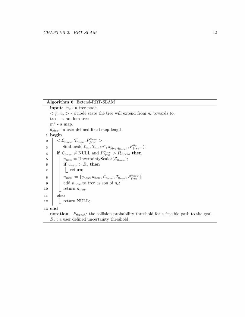
CHAPTER 2. RRT-SLAM 42
Algorithm 6: Extend-RRT-SLAM
input: nc - a tree node.< qr, ur > - a node state the tree will extend from nc towards to.tree - a random treem∗ - a map.dstep - a user defined fixed step lengthbegin1
< Lnnew ,Tnnew , Pnnew
free > =2
SimLocal( Lnc,Tnc ,m∗, π[qns ,qnnew ]
, Pnc
free, );3
if Lnnew 6= NULL and Pnnew
free > Pthresh then4
unew = UncertaintyScalar(Lnnew);5
if unew > Bu then6
return;7
nnew := {qnew, unew,Lnnew ,Tnnew , Pnnew
free };8
add nnew to tree as son of nc;9
return nnew10
else11
return NULL;12
end13
notation: Pthresh: the collision probability threshold for a feasible path to the goal.Bu : a user defined uncertainty threshold.
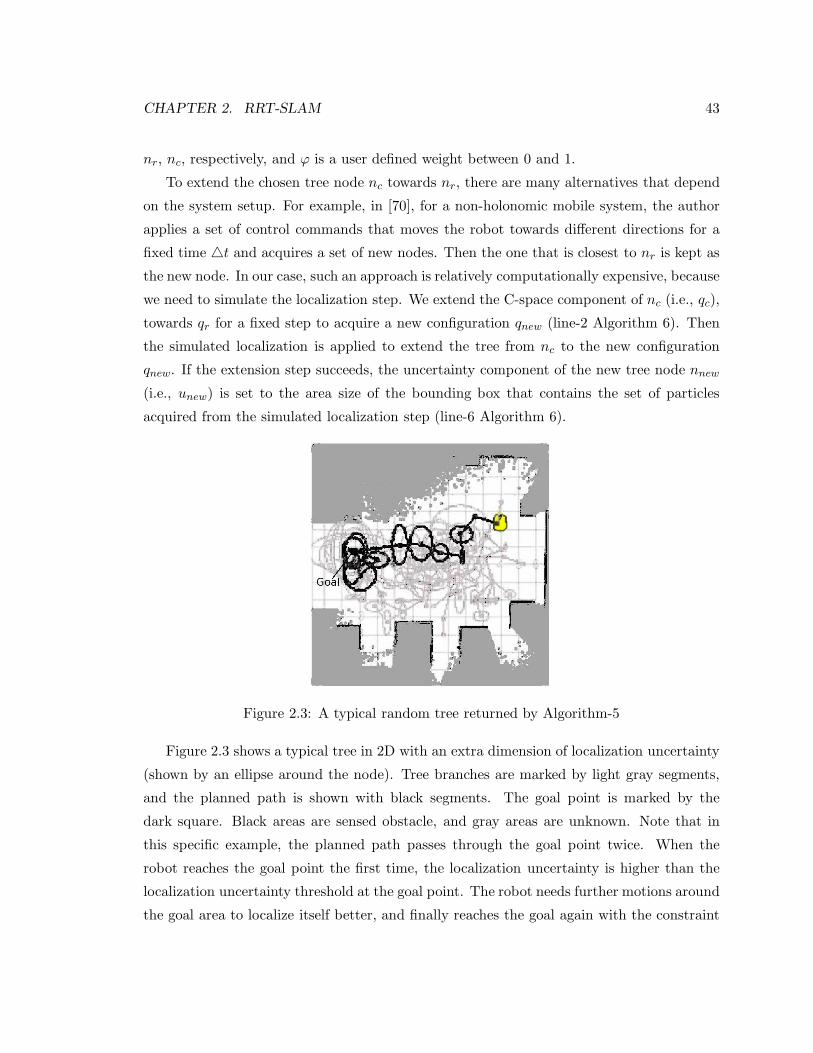
CHAPTER 2. RRT-SLAM 43
nr, nc, respectively, and ϕ is a user defined weight between 0 and 1.
To extend the chosen tree node nc towards nr, there are many alternatives that depend
on the system setup. For example, in [70], for a non-holonomic mobile system, the author
applies a set of control commands that moves the robot towards different directions for a
fixed time △t and acquires a set of new nodes. Then the one that is closest to nr is kept as
the new node. In our case, such an approach is relatively computationally expensive, because
we need to simulate the localization step. We extend the C-space component of nc (i.e., qc),
towards qr for a fixed step to acquire a new configuration qnew (line-2 Algorithm 6). Then
the simulated localization is applied to extend the tree from nc to the new configuration
qnew. If the extension step succeeds, the uncertainty component of the new tree node nnew
(i.e., unew) is set to the area size of the bounding box that contains the set of particles
acquired from the simulated localization step (line-6 Algorithm 6).
Figure 2.3: A typical random tree returned by Algorithm-5
Figure 2.3 shows a typical tree in 2D with an extra dimension of localization uncertainty
(shown by an ellipse around the node). Tree branches are marked by light gray segments,
and the planned path is shown with black segments. The goal point is marked by the
dark square. Black areas are sensed obstacle, and gray areas are unknown. Note that in
this specific example, the planned path passes through the goal point twice. When the
robot reaches the goal point the first time, the localization uncertainty is higher than the
localization uncertainty threshold at the goal point. The robot needs further motions around
the goal area to localize itself better, and finally reaches the goal again with the constraint

CHAPTER 2. RRT-SLAM 44
on the localization uncertainty at the goal less than the required threshold.
(a) path1
(b) path2
Figure 2.4: The same goal but different goal uncertainties were given to the robot. Thepaths found were different. For the low uncertainty case (b), robot prefers to go closer toknown obstacles to localize itself better.
2.4 Simulations
We have run preliminary tests in our simulated test-bed. We acquire online [71] the open
source code and libraries implementation (referred as Gmapping [72]) of FastSLAM, and
incorporate them in our RRT-SLAM implementation. We use the collision detector that is
incorporated in the Player-Stage library [73].
To show meaningful examples, we manually set a sequence of intermediate goal positions,

CHAPTER 2. RRT-SLAM 45
moving the robot along these positions while executing SLAM to explore the simulated
environment. In this subsection, the range sensor in the simulated environment is 4 meters.
and the environment size is indicated by grids shown in the map, with each grid of size 1
meter by 1 meter.
A typical scenario, which indicates the effectiveness of our RRT-SLAM during the ex-
ploration is shown in Figure 2.4, where the robot needs to go across the open free area with
a collision probability less than 0.15 (chosen somewhat arbitrarily 6). The goals in Figure
2.4(a) and Figure 2.4(b) are at the same location but the uncertainty threshold at goal in
Figure 2.4(a) (0.8) is much larger than in Figure 2.4(b) (0.2). In the UC-space, they cor-
respond to two different points separated along the uncertainty dimension. Our algorithm
returns paths that satisfy the collision probability threshold along the path(s) and the lo-
calization uncertainty threshold at the goal. Note that even though path1 is shorter than
path2, the localization uncertainty along the first path is higher than the second path, and
the collision probability for the first path (0.023) is higher than the second path (0.0). Here,
the higher probability of collision for the first path is mainly due to the localization uncer-
tainty around the third last path node. We do not explicitly show the state particle sets
along the path in Figure 2.4, but use the ellipse to demonstrate the localization uncertainty
at each tree node along the path.
Figure 2.5 shows the advantage of applying RRT-SLAM compared with the classic RRT
without considering the localization uncertainty. For the path returned by the classic RRT
we also simulate the localization uncertainty and calculate the expected collision probabil-
ity. The collision probabilities for the paths in Figure 2.5 (a) and (b) are 0.0 and 0.82,
respectively.
Clearly, RRT-SLAM gives a more robust path than the classic RRT because the latter
searches for the path in the C-space without considering the localization uncertainty, and
hence might increase the chance for the robot to collide with the environment.

CHAPTER 2. RRT-SLAM 46
(a) A solution path returned by (b) A solution path returned by standard RRTRRT-SLAM. in our simulated test-bed, with no
uncertainty and collision probabilitytaken into consideration.
Figure 2.5: Comparing solution paths returned by RRT-SLAM and the classic RRT in thesimulated environment.
2.5 Experiments
We also implemented RRT-SLAM on a real PowerBot system. The Hokuyo URG-04LX
range scanner having a sensing range of 4.0m and a span angle of 180◦, is fixed on the
PowerBot and points to the front. The on-board computer has an IntelTM
CPU of 3.0GHz,
with RedhatTM
Linux installed.
Again, we first manually set a sequence of intermediate goal positions, moving the robot
along these positions while executing SLAM to explore the real environment. Figure 2.6
shows this partially constructed map of RAMP lab in Applying Science Building at SFU.
The size of the map is about 7x7 meters. In the task shown in Figure 2.6, the robot tries
to get to the end of the corridor for further exploration.
Figure 2.7 (a) and (b) show the paths returned by RRT-SLAM and classic RRT (with
collision probability of 0.0 and 0.21), respectively. This result clearly shows that path
6Intuitively, allowing a path with non-zero probability of collision and higher localization uncertaintytends to reduce the difficulty level of the planning problem. In practice, the specific threshold would beexperimentally determined by the user.

CHAPTER 2. RRT-SLAM 47
Figure 2.6: A map of the RAMP lab in the Applied Science Building at SFU. The next goalof the robot is marked.
(a) A solution path returned by (b) A solution path returned by the classicRRT-SLAM in real environment. RRT in in real environment, with no
uncertainty and collision probabilitytaken into consideration.
Figure 2.7: Comparing solution paths returned by RRT-SLAM and the standard RRT inthe RAMP lab environment shown in Figure 2.6.

CHAPTER 2. RRT-SLAM 48
Figure 2.8: Trace of the mobile base as it executes the path planned using RRT-SLAM forthe RAMP lab environment.
returned by the RRT-SLAM gives the robot more clearance (especially in the horizontal
corridor area), and therefore is safer compared to the path returned by the classic RRT.
Finally, the robot successfully executed the path planned by RRT-SLAM (Figure 2.7
(a)) and reached the goal. The trajectory of the robot is plotted in Figure 2.8.
2.6 Parameter Values Related to RRT-SLAM
Unless specified otherwise, we used the parameter values that are listed in Table 2.1 for
all the simulations and experiments about RRT-SLAM and its variation i.e., RRT-FD (ex-
plained in detail in next chapter). These parameters are divided into two groups. The first
group of parameters are related to the simulated localization step, where ♯L is the number
of state particles; σd and σθ are the standard deviations of the motion error for translation
and rotation, respectively; εθ is used to determine whether robot’s next motion includes
translation or not(Equation 2.5). The parameters in the second group are applied to RRT-
SLAM, where dstep (line-2 Algorithm 6) is the fixed step length for each RRT extension in
the C-space component; ϕ is the weight of the distance metric in UC-space for RRT-SLAM
(Equation 2.16); Bu is the largest uncertainty allowed for a tree node; Pthresh is the collision-
free probability threshold for a feasible path to the goal, and Bugoalis the goal uncertainty
threshold. In the planning stage, the collision detector is called every time the simulated
motion of the robot rotates (or translates) a fixed angle △θcol (or distance △dcol).

CHAPTER 2. RRT-SLAM 49
Simulated localization RRT-SLAM
♯L σd σθ εθ
30 0.01m 0.015o 5◦dstep ϕ Bu Pthresh Bugoal
△θcol △dcol
0.8m 0.2 2.0 m2 0.90 0.15 5o 5cm
Table 2.1: Parameter values applied in RRT-SLAM for the simulations and experiments.Unless specified otherwise, all simulations and experiments used these values.
2.7 Discussion
In our RRT-SLAM implementation, each time a tree node is extended, we need to simulate
the localization process, which is time consuming (takes up to around 0.5 second to extend
a tree node in our simulation and experiments). Therefore in the RRT-SLAM framework,
which embeds only the standard RRT technique, an efficient tree node generation [6] be-
comes important. This motivates us to further study the RRT efficiency in the UC-space,
which is the major interest in next chapter.

Chapter 3
RRT-SLAM-FD: Fractal
Dimension Based RRT-SLAM in
the UC-Space
In Chapter 2, we presented RRT-SLAM, a RRT based motion planning technique that incor-
porates robot localization uncertainty and mapping uncertainties. The algorithm searches
for a path in the UC-space. We now discuss the efficiency issue of RRT-SLAM in the
UC-space.
3.1 Tree Exploration in the Uncertainty-Configuration Space
(UC-Space)
In RRT-SLAM, the localization uncertainty component of a new tree node is acquired by a
the simulated localization step using the current best map (refer to Chapter 2 for detail).
That means the uncertainty component of a new tree node is determined not only by the
uncertainty of its father node and the control command a, but also by the current best map
and the localization algorithm applied. Consequently, the true distance, i.e., the length of
the optimal path, between two tree nodes in the UC-space, can hardly be measured by the
traditional weighted Euclidean distance metric. Since RRT is well known for it sensitivity
to the applied distance metrics [6], the “rapid” flavor of the RRT tends to be compromised
in the UC-space.
50

CHAPTER 3. RRT-SLAM-FD 51
3.1.1 Classic RRT’s Dependence on Metrics
We now briefly review why the classic RRT is sensitive to the distance metric applied.
In each iteration, RRT aims to place the new tree node nnew, in an area that is not yet
“covered” by the tree. To achieve this, RRT first randomly generates a node (denoted as
nr). Since the larger the uncovered area is, the higher the probability for nr being placed
in this area. Intuitively, this random node actually “identifies” the area that is not covered
by the tree.
Next, RRT tries to extend the tree “towards” the random generated node nr, or equiv-
alently, the uncovered area. However, finding the optimal solution, i.e., the optimal path
from current tree nodes to nr, is as hard as solving the original motion planning problem.
RRT picks up the tree node that is the “closest” to nr using a distance metric defined over
tree nodes as a heuristic, and extends the tree from the chosen tree node “towards” the
random node. That means nr is inside the Voronoi region of the chosen tree node. In other
words, those tree nodes that have larger Voronoi region tend to be chosen to extend at each
iteration, the so-called Voronoi-bias [74].
Obviously, tree nodes that are “close” (measured by the distance metric applied) to the
uncovered area tend to have higher chance to be chosen to extend. However, extensions
from these nodes may lead new nodes to be generated in the area that has been covered by
the tree, if the distance metrics does not reflect the true distance between tree nodes. Also
these tree nodes might be chosen numerous times, which leads to inefficient node generation
[34].
For systems such as rigid body and open-chain, commonly used distance metrics, such
as the weighted Euclidean, works well [23], because the robot can move along a straight line
in the C-space from the chosen node towards the random node , i.e., the distance reflects
the shortest path taken modulo the presence of obstacles. This means that getting closer to
the random node from the chosen tree node is an easy task unless the robot is occluded by
obstacles. Therefore a new node is more likely to be inside the father node’s Voronoi region,
which is a large empty area that has not yet explored by the tree, hence achieving efficiency.
But clearly this is not the case for RRT in the UC-space, because the uncertainty component
of a new node, as mentioned before, also depends on the environment. Consequently, there
is no easy solution to move “towards” the random node from the chosen tree node, and it
is also hard to predict where the new node will be located(in our case due to unpredictable

CHAPTER 3. RRT-SLAM-FD 52
change in uncertainty), hence compromising the efficiency of RRT.
3.1.2 RRT-Blossom
RRT-Blossom (Algorithm 7), instead of looking for a “better” distance metric, aims to
reduce the RRT’s sensitivity on the applied distance metric. An illustration of the algorithm
[24] is shown in Figure 3.1. Let nodes na and nb be the latest two nodes added into the tree.
However, nb does not contribute much to the tree exploration (or, equivalently, nb is deemed
in areas that has already been covered by the tree). This case is referred to as “regression”
(we will discuss the precise condition later in Section 3.1.3 and 3.2). So RRT-blossom forbids
(temporarily) further extension from nb, and nb is referred to as the “dormant” node (light
colored). na, on the other hand, contributes “well” and is referred to as “live” nodes (dark
colored). RRT-blossom allows only those live nodes to be extended in further iterations.
To understand RRT-Blossom, as shown in Figure 3.1, one way to interpret it is that
the set of live nodes is a coarse representation of the whole tree. This means that RRT-
blossom searches first at a lower resolution, and avoids spending time on extending from
those dormant nodes at local areas, hence leading to efficiency.
If those dormant nodes are necessary to the solution path, RRT-Blossom will later wake
them up (i.e., turn the dormant status into live), and allow further extensions from them.
To achieve this, the authors introduce a state-transition machine, where a tree node state
will transit among one of the three states: live, dormant, dead. Each time a new node is
acquired, it will be marked as dormant or live subject to the regression checking condition.
A node is dead if all of its sons are either dead or collided with obstacles. A dormant node
will be waken up if the blocking node (i.e., the node closest to the dormant node, at the time
the dormant node is generated, referring to the part about the regression checking condition
below) is dead or the child of the dominant node is waken up. Finally, in RRT-Blossom,
each node is allowed to be extended for a fixed number of times (we use 8 throughout our
work).
The basic idea of RRT-Blossom can be easily incorporated into RRT-SLAM, and hence
addresses the efficiency issue in the UC-space. We name this modified RRT-SLAM ver-
sion as RRT-SLAM-Blossom. Note that in our RRT-SLAM-Blossom, when extending the
chosen tree node towards the random node, we extend the C-space component of nc (i.e.,
qc), towards qr for a fixed step to acquire a new configuration qnew. Then, the simulated
localization is applied to extend the tree from nc to the new configuration qnew (refer to

CHAPTER 3. RRT-SLAM-FD 53
RRT-SLAM for detail).
Algorithm 7: One iteration of tree extension in RRT-Blossom [24].
begin1
nr := random state()2
nc := nearest neighbor(nr, tree)3
for a ∈ A do4
nnew = sim(nc, a)5
if fail(nc, a, nnew) OR reg.(nc, a, nnew) then6
continue7
tree = tree + new edge(nc, a)8
return a new node closest to nr.9
end10
notation:a: a motion command.A: a discretized motion command set.
Free Area
na
Obstacle
nb
nsnr
Figure 3.1: The regression checking mechanism for RRT-Blossom.
3.1.3 Original Regression Condition in the UC-Space
The regression checking is crucial to RRT-Blossom [24]. It is indeed a measurement of the
new node’s “contribution” to the tree’s exploration progress in the space searched, and keeps
those nodes that “contribute well” (i.e. non-regression nodes) as live nodes. [24] proposes
a regression checking condition, shown in Equation 3.1. It basically says that a new node is
in regression if it is outside the Voronoi region of its father node (in other words, the node
closest to the new node is not the father node, and this closest node is referred to as the
“blocking” node).

CHAPTER 3. RRT-SLAM-FD 54
reg.(nc, nnew, tree) :
∃n ∈ tree, such that ρ(n, nnew) < ρ(nc, nnew)(3.1)
As described in [24], Equation 3.1, which aims to detect redundant explorations, is a
practical solution that works effectively in their system setup (two typical systems including
a non-holonomic system and a kinodynamic system). However, we should notice that this
approach is heuristic based. The effectiveness of applying Equation 3.1 to detect redundant
explorations depends heavily on the distance metric applied ρ(.). We now discuss why
Equation 3.1 would perform poorly in the UC-space.
x
un ertainty
nr
nnew
nc a
Figure 3.2: Failure of the original regression condition in the UC-space.
Now consider a toy example of RRT in the UC-space as shown in Figure 3.2. The robot
has one degree of freedom and moves along x axis with motion uncertainty. The 1D on-
board range sensor helps the robot to localize itself by detecting the markers (black stars)
in the environment. Here, an extra dimension of uncertainty is indicated by the vertical
axis. In Figure 3.2, nc is chosen to be extended towards the randomly generated node
nr by applying a motion command a. If the localization algorithm successfully reduces

CHAPTER 3. RRT-SLAM-FD 55
localization uncertainty, the new node will be in position nnew (with low uncertainty),
outside the Voronoi region of nc, i.e., the father node. Hence it will be reported as regression
and marked as dormant (3.1). Intuitively, nnew in Figure 3.2 contributes well to the tree
expansion process in the UC-space, and should be kept as a live node.
The situation as shown in Figure 3.2 could arise frequently when the robot with higher
localization uncertainty approaches features in the environment. In other words, the original
regression condition tends to put more new nodes into the dormant state than necessary in
the UC-space.
To illustrate what has been discussed in Figure 3.2, we give in Figure 3.3 an example.
In this subsection, all the figures are acquired in the environment setup as shown in Figure
3.9 for Problem B (refer to Section 3.4). We generate a random tree by applying the RRT-
SLAM-Blossom mechanism in the UC-space after a small number of iterations, and show
the nodes that are non-regression (live nodes) as determined by Equation 3.1. Obviously,
the live nodes tend to be closer to their fathers (i.e., do not have dramatic changes in the
uncertainty component). The main reason is that, similar to the discussion about Figure
3.2, those new nodes out of their fathers’ Voronoi regions (due to the dramatic change in
the uncertainty component, and therefore far away from their fathers) will be reported as
in regression if the original regression is applied.
Figure 3.3: The live tree nodes picked by the regression condition (Equation 3.1) introducedin RRT-blossom.
In Figure 3.4, we illustrate both the live nodes (dark colored) and the dormant nodes
(light colored) for RRT-SLAM-Blossom. As mentioned before, this set of live nodes is
preferably a coarse representation of the area that has been covered by the tree (refer to the

CHAPTER 3. RRT-SLAM-FD 56
explanation to Figure 3.1), such that RRT-Blossom can search first in a coarse resolution.
However, as a consequence of the aforementioned shortcoming of the original regression
checking condition, the live nodes identified using the original regression condition cover
only a limited portion of the area that has been covered by the tree.
Figure 3.4: Distribution of the live nodes (dark) under the original regression condition.The dormant nodes are shown in light color.
Another drawback when applying the original regression condition in the UC-space is
shown in Figure 3.5. Because many tree nodes are “mistakenly” marked as dormant, we
observe that the number of live nodes that are available for further extension might be
very small (as mentioned before, in RRT-SLAM-Blossom, a live node extended more than
8 times will not be considered in further extension). In Figure 3.5, the live nodes available
for further extension are in dark color, and otherwise are in light color. This tends to cause
RRT-SLAM-Blossom to spend time on searching at some particular local areas around those
available live nodes. Since it is hard to predict where this small amount of available live
nodes will appear in practice, this becomes problematic when there are some key areas that
require more attention, but those available live nodes do not appear in these areas even
after many iterations.
With these drawbacks of the original regression checking condition in mind, we now
propose a new regression checking mechanism that works well in the UC-space.

CHAPTER 3. RRT-SLAM-FD 57
Figure 3.5: An example of applying the original regression checking condition (Equation3.1) in the UC-space. Only live nodes are shown. A small number of live nodes (darkcolored) are available for further extensions. Nodes in gray color are also live nodes, butthey have been extended more than 8 times and hence will not be further extended (referto the explanation for RRT-Blossom).
3.2 Outlier Detection Mediated Regression Checking
Since regression checking is used to answer whether a new tree node is being placed in an
area that is not yet “covered” by the tree nodes, it could be treated as an outlier w.r.t.
the set of existing tree nodes. Thus, the regression checking indeed becomes an outlier
detection problem from sequential data clustering point of view [25]. Several criteria have
been used for outlier detection in sequential data clustering literature [75]. We choose to
use the Fractal Dimension (FD) of a data set.
3.2.1 Fractal Dimension
The fractal dimension is originally used to characterize fractal sets, i.e., structures that
appear as a consequence of self-similarity. In research areas such as information theory,
data mining, etc., the fractal dimension is used to measure a data set’s intrinsic dimension,
which reflects self-similarity of the data set.
The fractal dimension is defined as follows [25]. Let di be a grid of size r in each
dimension in an n-dimensional space, and pi be the frequency of the data points fall into
the cell di. The generalized fractal dimension Dq is defined as:
Dq =1
q − 1
∂ log∑
i pqi
∂ log r. (3.2)
In particular, the Hausdorff fractal dimension (q = 0), the information dimension

CHAPTER 3. RRT-SLAM-FD 58
limq→1Dq, and the correlation dimension (q = 2) are widely used. In this work, we se-
lect q = 1, i.e., the information dimension, “which is the entropy and therefore reflects
changes in trends” [25], and denote it as FD.
3.2.2 Applying FD as a Regression Condition
Whether a new datum is an outlier of the data set could be well detected based on the
change of the FD value after the new datum is included in the data set. Our new FD based
regression checking condition is given by,
reg.FD(nc, nnew, tree) :
if ∆f < fthresh AND reg.(nc, nnew, tree)(3.3)
where ∆f is the change in the FD value for the tree node set before and after the new node
is included in the tree, and fthresh is a user defined threshold. Equation 3.3 basically claims
that a new node is in regression if the original regression condition is satisfied AND the FD
value of the tree node set (with the new node included) does not increase significantly, i.e.,
the increment is less than a user defined threshold after a new node is included in the tree.
The complexity of calculating FD is of N log N , where N is the size of the data set
[25]. When we extend the random tree in the UC-space, the most computationally time-
consuming step, at each iteration, is in the simulated motion step, which uses the simulated
SLAM and is much more significant compared to the cost of FD calculation. As shown below
in our simulations, even though the FD based regression checking introduces extra cost of
N log N at each iteration, it results in an efficient node generation, hence still improving
the overall efficiency.
3.3 Improving RRT-SLAM Efficiency in the UC-Space: RRT-
SLAM-FD
The detailed RRT-SLAM-FD algorithm is given in Algorithm 8 and 9. There are two major
differences between RRT-SLAM-FD and RRT-Blossom.
The first distinction between RRT-SLAM-FD and RRT-Blossom is, of course, the re-
gression checking mechanism applied (line-11 Algorithm 9).

CHAPTER 3. RRT-SLAM-FD 59
Algorithm 8: RRT-SLAM-FD
input: Y - SLAM particle set before robot planning the motion.output: tree - a random tree.begin1
< q∗,m∗b > := the most weighted particle in Y;2
for i = 1 to ♯L do3
q[i]ns = q∗; ω
[i]ns =
[i]ns = 1
♯L4
Pns
free = 1;5
tree.init(qs, us = 0,Lns , T Lns
, Pns
free);6
DEADNUM COUNT = 87
k = 2, e num = 0, prev e num = 08
w num = 0; prev w num = 09
while !TimeUp() and !(ReachGoal()) do10
< qr, ur >:= RandomState() ;11
nc := NearestNeighbor(< qr, ur >, tree);12
qnew = ExtendTo(qnc , qr, dstep);13
Extend-RRT-SLAM-FD(tree, qnew, nc,m∗b);14
e num = getExtensionNum()15
w num = getLiveNodesNum()16
if e num > prev e num + k then17
if w num <= prev w num then18
fthresh = fthresh − fstep19
k + +20
if k >= DEADNUM COUNT then21
k = DEADNUM COUNT22
else23
fthresh = fthresh + fstep/224
prev w num = w num25
prev e num = e num26
end27
notation: q[i]nj : the ith particle in Lnj
.
ω[i]nj : the weight of q
[i]nj .
[i]nj : the weight of ith trail particle stored in Tnj
.Tnj
: a data set stored at tree node nj.

CHAPTER 3. RRT-SLAM-FD 60
Algorithm 9: Extend-RRT-SLAM-FD
input: nc - a tree node.qnew - a configuration, towards which the tree will extend from nc.tree - a random treem∗ - a map.dstep - a user defined fixed step.begin1
< Lnnew ,Tnnew , Pnnew
free > =2
SimLocal( Lnc,Tnc ,m∗, π[qns ,qnnew ]
, Pnc
free, );3
if Lnnew 6= NULL and Pnnew
free > Pthresh then4
unew = UncertaintyScalar(Lnnew);5
if unew > ubound then6
return;7
else8
nnew := {qnew, unew,Lnnew ,Tnnew , Pnnew
free };9
if reg.FD(nc, nnew, tree) then10
return;11
else12
add nnew to tree as son of nc;13
else14
return;15
end16
notation: Pthresh: the collision probability threshold for a feasible path to the goal.ubound : a user defined uncertainty threshold.

CHAPTER 3. RRT-SLAM-FD 61
Secondly, RRT-SLAM-FD is different from RRT-Blossom in how to deal with the dor-
mant nodes. As previously discussed, if those dormant nodes are crucial for the solution
path, RRT-blossom wakes those dormant nodes, and searches at a finer resolution for al-
ternative paths. RRT-blossom wakes a dormant node (as well as all its precedents that are
dormant) based on the very local information around this node: a dormant node is waken
when a nearby live node is dead, i.e., all the extensions from this live node are failed, or all
its descendants are dead. Therefore, as reported by the authors, the planner might “spend
much time unnecessarily exhausting the free-space” before these dormant nodes, which are
keys to the solution path, are waken up.
Our solution to the above issue is that, instead of waiting for the dormant node to
be waken up, we reduce the FD threshold adaptively. With a reduced threshold, a new
node that “contributes” less to the tree exploration (which would have been deemed as in
regression before fthresh is reduced) will be kept as the live node. So the new live node will
be generated close to the dormant node. The motivation of waking the dormant node is,
indeed, to search for alternative paths at a finer resolution, so reducing the FD threshold
has the similar effect to waking the dormant node up.
Intuitively, we should search at a finer resolution, when the tree stops making progress
at current resolution, which could be well indicated by checking whether the new nodes are
frequently in regression (new nodes often in the area that has been covered by the tree) in
the next few iterations. Or equivalently, it could be reflected by the amount of decrease
of the number of nodes that are both live and available for extension. In our work, we
control the increment of “searching resolution” by monitoring the change of the number of
live nodes available for extension.
In RRT-SLAM-FD, after k extensions, we check the number of available live nodes wnum
(line-17 Algorithm 8). If wnum does not increase, we reduce the FD threshold by a fixed
step, fstep, to increase the search resolution. If wnum does increase (line-23 Algorithm 8),
to avoid the resolution to increase too rapidly, we increase the threshold by a small amount
(set as half of fstep so that the overall trend of the threshold keeps dropping). Users can
control the increment speed of search resolution by adjusting the value of k. k is initially
set to a low value, and is progressively increased each time the threshold is decreased. The
higher k is, the slower the increment speed of search resolution. Note that we bound the
value of k to avoid the search resolution to increase too slowly. In our case, we set its value
between 2 and 8, which is the maximum number of extensions allowed for one node.

CHAPTER 3. RRT-SLAM-FD 62
3.3.1 Discussions on RRT-SLAM-FD
As previously illustrated in Figure 3.2, the original regression condition may fail to work
properly in the UC-space. Here, we show the effectiveness of the new regression condi-
tion with specific examples. Again, in this subsection, all the figures are acquired in the
environment setup as shown in Figure 3.9 for Problem B (refer to Section 3.4).
Figure 3.6 shows the nodes that are non-regressive (live nodes) after applying RRT-
SLAM-FD, as determined by the new regression condition (Equation 3.3). Our FD based
regression checking condition treats many nodes out of their fathers’ Voronoi regions as the
live nodes, and therefore many long branches appear due to the change of the uncertainty
component w.r.t. the father node (refer to Figure 3.3 for a comparison).
Figure 3.6: The live tree nodes picked by the new FD based regression condition (Equation3.3).
Figure 3.7: Distribution of the live nodes under the new FD based regression condition.

CHAPTER 3. RRT-SLAM-FD 63
Figure 3.7 illustrate both the live nodes (dark colored) and the dormant nodes (light
colored). Comparing to the original regression condition (Figure 3.4 shown in Section 3.1.3),
the nodes picked by the FD based regression condition are distributed in a more uniform
fashion, and hence provide a better coarse representation of the whole tree. As mentioned
before, preferably, those chosen live nodes should be a coarse representation of the area that
has been covered by the tree such that RRT-Blossom can search first in a coarse resolution
(refer to the explanation to Figure 3.1). Clearly, RRT-SLAM-FD keeps this very spirit of
RRT-Blossom in the UC-space.
3.3.2 Box Counting: an Algorithm to Determine FD
In our work, we adopt the box counting algorithm as described in [25], and address some
issues regarding this algorithm used to calculate the FD value.
The box counting algorithm divides the space into cells of size r, and counts how many
cells are occupied by data set points denoted as N(r). A plot of N(r) versus r is created,
and the slope of the plot is the Hausdorff FD. Other fractal dimensions could be acquired
in a similar fashion.
The box counting algorithm needs a data set of enough size in order to find a meaningful
slope of the line that fits N(r) and r. Therefore, for the box counting to return a value as a
meaningful approximation of FD, the size of the data set has to be larger than a threshold,
which increases exponentially with the dimensionality of the data set [76]. Thus in the
first several iterations of RRT (experimentally around the first 400-600 iterations in our 3
dimensional UC-space), the FD value returned by the box counting algorithm should be
discarded.
To address this issue, we generate (somewhat arbitrarily) an initial data set (the size is
1000) in the UC-space. For each data, the C-space component is randomly generated, and
the uncertainty-component is a constant, which is 2.0 times the largest uncertainty allowed
for a tree node. One can imagine the initial data set as a layer of cloud on the top of all tree
nodes. How the initial data set is arranged (position, shape, etc.) will affect the FD value
at each iteration. However, this will not be a concern in practice because we care about just
the FD difference (∆f) at each iteration.
Figure 3.8 shows how the FD value of a data set, including the tree nodes plus the initial
data set, changes at each iteration of RRT-SLAM-FD in the UC-space for 5 runs (acquired

CHAPTER 3. RRT-SLAM-FD 64
Figure 3.8: FD values for the data set of the RRT-SLAM nodes, with the initial data set inthe UC-space, for 5 runs.
in the environment as shown in Figure 3.9, Problem B). In each run, we run RRT-SLAM-
FD, record the FD value at each iteration, and plot these values as one curve in Figure 3.8.
The first observation is that adding a new node tends to increase the FD value. Secondly, we
can see that the increment of FD value tends to be larger at the earlier iterations. The main
reason is that, in later iterations, most of the places have been covered by the tree, and hence
the new node tends to “contribute less” than those in earlier iterations. This also indicates
that the change of the FD value could indeed be a measurement of the “contribution” to
the tree expansion for each tree node.
3.4 Simulations
We test our RRT-SLAM-FD in our simulated test-bed and compare it with RRT-SLAM
and RRT-SLAM-Blossom in three problems as shown in Figure 3.9 and 3.10, where the
white area, the black areas, and the gray areas represent the free, known obstacles, and
unknown areas, respectively. We assume that the robot is in the middle of exploration task,
and needs to go to another place to continue the exploration. In the first problem, the goal
is set at A in Figure 3.9, which is closer to the relatively large open region, but is further
away from the known obstacles. The second problem needs the robot to reach position B,
which is surrounded by the unknown areas (hence in a narrower space, since robot can not

CHAPTER 3. RRT-SLAM-FD 65
Figure 3.9: Problems A and B.
Figure 3.10: Problem C.

CHAPTER 3. RRT-SLAM-FD 66
enter the unknown areas) in Figure 3.9, and is closer to the known obstacles than A. In
the third problem (Figure 3.10), we have a larger environment size of 16 by 12 meters (the
environment in Figure 3.9 is about 9 by 7 meters), and larger free space than Figure 3.9.
The goal point C is in open free region.
We show in Figure 3.11 (a), (b) and (c), the tree structures acquired with RRT-SLAM,
RRT-SLAM-FD and RRT-SLAM-Blossom, respectively, for Problem, C. For RRT-SLAM-
FD and RRT-SLAM-Blossom, nodes and branches in dark (gray) color are respectively
the live (dormant) nodes and branches. We observe that both RRT-SLAM-blossom and
RRT-SLAM-FD only allow a portion of the nodes to be further extended, hence avoiding to
spend much time at local areas, which is the major difference from RRT-SLAM in achieving
efficiency. We also observe how the FD based regression checking impacts on the selection
of the live nodes (Figure 3.11 (c)), compared to the original regression condition in RRT-
SLAM-blossom (Figure 3.11 (b)). First, in Figure 3.11 (b3), we can tell that the uncertainty
difference between a live node and its father tends to be small. A new node that has dramatic
change of localization uncertainty, w.r.t. its father node tends to be marked as the dormant
by RRT-SLAM-blossom (refer to Section 3.3.1 for detail). Secondly, the original regression
condition leaves many local areas without a single live node (marked by hand as A, B,
C in Figure 3.11 (b2)), which means that the exploration in these local areas is limited.
RRT-SLAM-FD clearly remedies these issues, hence successfully improving efficiency in the
UC-space.
We performed 60 trials for each algorithm in all three problems. Table 3.4 shows the
number of tree nodes N , the number of extension failures (Nfail), time taken (all in av-
erages) to solve each problem for RRT-SLAM, RRT-SLAM-blossom and RRT-SLAM-FD,
respectively. The variance of the time taken and the average time spent on the FD calcula-
tion are listed as well. The parameters in RRT-SLAM-FD is as follows: fthresh is initially
set at 0.00022; fstep is 0.000003. These parameters are kept the same in all runs.
We can see that the performance of RRT-SLAM-blossom is hard to predict due to the
fact that the original regression condition does not fit properly in the UC-space. In our sim-
ulations for Problems A and B, RRT-SLAM-blossom is even outperformed by RRT-SLAM,
while in simulation for Problem C, RRT-SLAM-blossom performes better than RRT-SLAM.
However, after switching to the new FD based regression condition, and adaptively adjusting
the FD threshold, our new RRT-SLAM-FD consistently shows performance improvements
in the UC-space for all the three problems.

CHAPTER 3. RRT-SLAM-FD 67
(a1) (a2)
(b1) (b2) (b3)
(c1) (c2) (c3)
Figure 3.11: Tree structures in the UC-space, shown in 2D view ((a1), (b1) and (c1)) and 3Dview (the rests), acquired by applying RRT-SLAM ((a1) and (a2)), RRT-SLAM-Blossom((b1), (b2) and (b3)) and RRT-SLAM-FD ((c1), (c2) and (c3)), for Problem C. For RRT-SLAM-Blossom and RRT-SLAM-FD, the nodes (branches) in black and gray color are thelive and dormant nodes, respectively. In (b3) and (c3), only live nodes are shown.

CHAPTER 3. RRT-SLAM-FD 68
Pro Alg. N Nfail Time(sec.) VarT TimeFD(sec.)
RRT-SLAM 686 399 163 18996 0A RRT-SLAM-Blossom 814 263 204 48485 0
RRT-SLAM-FD 500 289 129 15102 7.4
RRT-SLAM 378 186 82 3075 0B RRT-SLAM-Blossom 700 179 166 21187 0
RRT-SLAM-FD 277 140 70 4270 3.5
RRT-SLAM 740 846 176 73345 0C RRT-SLAM-Blossom 772 161 134 13784 0
RRT-SLAM-FD 446 207 86 6693 7.0
Table 3.1: Simulation results for Problems A, B and C.

Chapter 4
Lazy-PRM for a Manipulator with
Base Pose Uncertainty
Represented by Particles
In this chapter, we consider the scenario, where the base is kept still while the on-board
manipulator is performing a motion in a given environment. However, the mobile base’s
true pose w.r.t. the environment might not be perfectly known due to the localization
uncertainty. We choose to extend PRM, instead of RRT, to plan the manipulator motion
because we aim to found a solution path of an optimal length. Correspondingly, the PRM
framework has to take this base pose uncertainty into the consideration.
4.1 Problem Formulation
We assume the manipulator motion can be precisely controlled. Also, the environment is
assumed to be known (or acquired via previous sensing). However, the manipulator base
pose (position and orientation) is not precisely known, and is represented with a set of N
weighted particles. Each particle indicates a possible base configuration qb = [x, y, θ], where
q[i]b is the ith particle. The weight of the ith particle, i.e., ω[i], represents the probability of
q[i]b being the true base configuration [7], with
∑Ni ω[i] = 1. Let q = [θ1, · · · , θd] ∈ Cm, the
C-space of the manipulator, be a configuration for the manipulator w.r.t. the base frame,
where d is the number of degrees of freedom of the manipulator. We use q[i] = [q[i]b , q] to
69
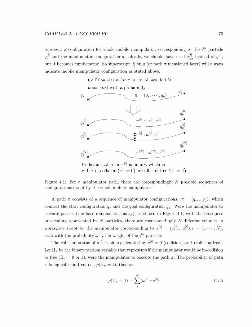
CHAPTER 4. LAZY-PRM-BU 70
represent a configuration for whole mobile manipulator, corresponding to the ith particle
q[i]b and the manipulator configuration q. Ideally, we should have used q
[i]bm instead of q[i],
but it becomes cumbersome. So superscript [i] on q (or path π mentioned later) will always
indicate mobile manipulator configuration as stated above.
qs
qg
π[0] : ω
[0], c
[0]
π[N ] : ω
[N ], c
[N ]
Collision status for π is not binary, but isasso iated with a probability.
Collision status for π[i] is binary, whi h iseither in- ollision (c[i] = 0) or ollision-free (c[i] = 1)
π[i] : ω
[i], c
[i]
q[0]s
q[i]s
q[N ]s
q[N ]g
q[i]g
q[0]g
π = (qs, · · · , qg)
Figure 4.1: For a manipulator path, there are correspondingly N possible sequences ofconfigurations swept by the whole mobile manipulator.
A path π consists of a sequence of manipulator configurations: π = (qs, ...qg), which
connect the start configuration qs and the goal configuration qg. Were the manipulator to
execute path π (the base remains stationary), as shown in Figure 4.1, with the base pose
uncertainty represented by N particles, there are correspondingly N different volumes in
workspace swept by the manipulator corresponding to π[i] = (q[i]s , ...q
[i]g ), i = (1, · · · , N),
each with the probability ω[i], the weight of the ith particle.
The collision status of π[i] is binary, denoted by c[i] = 0 (collision) or 1 (collision-free).
Let Ππ be the binary random variable that represents if the manipulator would be in-collision
or free (Ππ = 0 or 1), were the manipulator to execute the path π. The probability of path
π being collision-free, i.e., p(Ππ = 1), then is:
p(Ππ = 1) =N
∑
i
(ω[i] ∗ c[i]) (4.1)

CHAPTER 4. LAZY-PRM-BU 71
We would like to extend PRM to plan a path for the manipulator with the base pose
uncertainty. To construct a roadmap G in Cm, we generate samples of the manipulator
configuration q ∈ Cm, and connect samples within a distance threshold, as in the standard
PRM construction [26]. A node n of G is a configuration for the manipulator (denoted
as qn), and edges between two nodes ni,nj (denoted as e[ni,nj ]) are line segments in Cm.
Note that the collision status for samples and edges of G are not binary, but are associated
with a probability of being collision-free, which can be easily calculated in a way similar to
Equation 4.1.
For a roadmap G, a path π that connects the start node ns and goal node ng is feasible,
if p(Ππ = 1) ≥ δ, where δ ∈ [0, 1] is a user defined threshold. The problem in the query
phase is to return an optimized solution path π∗:
π∗ = argminπ
C(π)
s.t. p(Ππ∗ = 1) ≥ δ
(4.2)
where C(π) is the length (or cost) of the path π. We refer to this problem as the collision
probability constrained shortest path problem (CP-CSPP).
4.1.1 Underlying Structure of PRM with Base Pose Uncertainty
The graph G is constructed in Cm. But it has an underlying structure, because of base
uncertainty. Corresponding to each node n and edge e of G, we use n[i], e[i] (e[i][nj ,nk]) to
denote a node or edge in the configuration space for the whole mobile manipulator (denoted
as Cbm), with the base pose indicated by the ith particle. G[i] denotes the graph composed
of nodes n[i] and edges e[i], and let G = {G[1], · · · , GN}. Therefore, for a roadmap G in Cm,
there exists correspondingly a set of N graphs in Cbm. Figure 4.2 shows an example, where
N = 3, the weight of each particle is set equal to 13 . The dashed lines in G[1], G[2] and G[3]
are edges in-collision, and the solid line are collision-free.
Let Πe be the binary random variable that the mobile manipulator is in-collision or
free (Πe = 0 or 1), were the manipulator to travel along the edge e. Note for a path π
in G consisting of a sequence of M edges (e1, e2, · · · , eM ), c[i] in Equation 4.1 is given by
c[i]e1 ∧ c
[i]e2 · · · , c
[i]eM
, where c[i]ej = 1(0) if e
[i]j is collision-free (in-collision). As a consequence, we
have:

CHAPTER 4. LAZY-PRM-BU 72
ng
ne
nc
nb
na
nd
n[2]s
n[1]s
n[3]s
n[1]g
n[3]g
ω[1] = ω
[2] = ω[3] = 1
3
ns
G[1]
G[2]
G[3]
n[2]g
roadmap G in Cm
δ = 0.6
G[1], G
[2], G[3] in Cbm
Figure 4.2: Roadmap G in Cm, and the corresponding graph set G = {G[1], G[2], G[3]}constructed in Cbm (N = 3).

CHAPTER 4. LAZY-PRM-BU 73
p(Ππ = 1) =
N∑
i
(ω[i] ∗ [c[i]e1
∧ c[i]e2· · · , c[i]
eM])
≤N
∑
i
(ω[i] ∗ c[i]ej
) = p(Πej= 1)
(4.3)
where ej ∈ π, j = 1, · · · ,M . Therefore, if p(Πe = 1) is lower than the threshold δ, the edge
e can not be a part of a feasible path. We call such an edge in the roadmap G, as “N-edge”
(“N” stands for edges that can not be part of solution), and the rest as “S-edge” (“S” stands
for edges possibly be part of the solution). To calculate p(Πe = 1) (second row of Equation
4.3), c[i]e for all the i = 1 · · ·N can be easily computed with a collision detector [77]. For
example, in Figure 4.2, if δ = 0.6, both e[nc,na] and e[nd,ne] are N-edges and the rest are
S-edges. In a similar way, we distinguish nodes in G as N-nodes and S-nodes, which again
can be easily determined by using a collision detector.
4.1.2 CP-CSPP: an NP-hard Problem
CP-CSPP is a particular version of the well known constrained shortest path problem
(CSPP) [27], which is finding the shortest path that satisfies a given constraint. In our
case, the constraint over the solution path is the probability of being free. Another version,
the weight-constrained shortest path (WCSPP) problem has been shown as NP-hard w.r.t.
the size of the graph [27]. In our case, the constraints have a strong underlaying structure,
which we exploit to show that CP-CSPP is NP-hard as well, but in terms of the number of
particles N . The technique is similar to that employed in [78] which shows the NP-hardness
of WCSPP. We now show the NP-hardness of CP-CSPP.
First, we transform CP-CSPP, the problem in Equation 4.2 into another form. Corre-
sponding to each graph G[i] ∈ G, we associate it with the ith particle weight, ω[i]. For each
G[i], i = 1, · · · , N , we check collision for the edges and remove those in collision. Each G[i]
is then a subgraph of the roadmap G.
Now, it is easy to see that, the problem shown in Equation 4.2 is equivalent to solving the
following problem (call it P): search for a subset G∗ ⊆ G, such that the shortest path that
is common to all the graphs in G∗ is the smallest of all, subject that the weight summation
of the graphs in G∗ is larger than the threshold δ.

CHAPTER 4. LAZY-PRM-BU 74
G∗ = argminG′⊆G
C(πcom∗G′ ),
s.t.∑
G[i]∈G∗
ω[i] ≥ δ(4.4)
where πcom∗G′ is the shortest path that is common to all the graphs in G′
.
We transform the PARTITION problem, known to be NP-complete, into an instance of
our problem P.
Suppose we have a set S with N elements and every element ai, i = 1, · · · , N has a
corresponding size s(ai) ∈ Z+, ai ∈ S,∑
i s(ai) = 2A. The PARTITION problem is to
find a partition of S into Sa and Sb, such that the summation of elements’ size in these two
subsets are equal to A.
Given the partition problem, construct an instance of problem P as follows. We first
construct a graph G as shown in Figure 4.3, with the start and goal node (ns,ng) at two
ends. G contains 3N edges and 2N + 1 nodes, and is composed of a sequence of adjacent
triangles sharing a vertex. For ith triangle, the three edges are of the same length (equal
to s(ai)). Then, we construct a set of N graphs G[i], · · · , G[N ] from the graph G, such that
G[1] = G \ e1, · · · , G[N ] = G \ eN . Also we set ω[i] = s(ai). The set of graphs is denoted by
G = {G[1], · · · , G[N ]}. Above steps can be done in polynomial time.
|ei| = s(ai)
e2e1ns
G eN−1 eNng
Figure 4.3: A graph G constructed to transform the PARTITION problem into CP-CSPP
The problem P instance then is to find a subset G∗ of G such that the weight summation,
of G∗ is no less than A, and C(πcomm∗G′ ), is minimized.
From Figure 4.3, we can tell that
C(πcomm∗G′ ) = 2A +
∑
G[i]∈G′
ω[i]. (4.5)
If there exists a partition for S = Sa ∪Sb such that the summation of the size in Sa and

CHAPTER 4. LAZY-PRM-BU 75
Sb are equal to A, we can easily determine G∗ = {Gi : ai ∈ Sa}, i.e., G∗ shares the same
index set as Sa. Based on Equation 4.5, the weight summation and C(πcomm∗G′ ) are exactly
A and 3A, respectively. This is the minimal path length we can get, thus we have a solution
for problem P.
If a solution exists for our problem P, i.e., we find G∗, there are two possibilities for its
weight summation. If the weight summation is higher than A, there is no solution for the
PARTITION problem. If the weight summation is exactly A, we will have a solution for
the PARTITION problem, such that Sa shares the same index set as G∗.
This shows that CP-CSPP is NP-hard.
4.1.3 Using the Labeling Algorithm to Solve CP-CSPP
We now introduce the labeling algorithm, with our specific variant, to solve CP-CSPP. The
detailed algorithm below is mainly based on what is described in [27]:
Let the roadmap graph be G = (V,E), which consists of a set of nodes V and edges E.
The start node and goal node are ns and ng, respectively. Let Ii be the index set of labels
on the graph node ni. Essentially, each k ∈ Ii corresponds to a path πki from the start node
ns to ni. Let the probability of being free for the path πki , i.e. p(Ππk
ni= 1), be denoted as
P ki , and the length of the path πk
i be Cki . The kth label at node ni is then a pair (P k
i , Cki )
that is associated with path πki .
Clearly, the number of paths to a node could be exponential (in terms of number of
nodes in the graph) in the worst case. To help reduce the search, two key concepts are used:
a) dominant: We say label (P ki , Ck
i ) dominates label (P li , C
li) if 1) Ck
i < C li , and 2) for
two paths πli and πk
i , for all j = 1, · · · , N if π[j],li is collision-free, π
[j],ki is collision-free as
well. Clearly, if (P ki , Ck
i ) dominates (P li , C
li), πl
i can not be a portion of the optimal solution
path π∗, since it can be replaced by πki , which has lower cost. The domination relationship
between two labels can be efficiently determined in O(N).
b) efficient: We will call a label (P ki , Ck
i ) as efficient if it is not dominated by any other
label at node ni and P ki ≥ δ.
The detailed algorithm is shown in Algorithm 10. The general idea is to maintain all
possible paths to each node, and to eliminate paths whose labels are not efficient. The set
of labels is maintained as a tree structure. We refer to it as the label tree. In InitLabeling()
(line-2, Algorithm 10), the first label is initialized at node ns, i.e., (P 1s , C1
s ) with P 1s = 1
and C1s = 0. Correspondingly, the root node of the label tree contains [(P 1
s , C1s ), ns].

CHAPTER 4. LAZY-PRM-BU 76
The algorithm proceeds iteratively from the start node/label. At each iteration, among
all the labels that have not been extended before, a label at node ni, (P ki , Ck
i ) is chosen (the
one with minimal cost), and is extended to all the neighbors of ni. This involves, for all
neighbors nj of ni, 1) computing the label (Pj , Cj), associated with the concatenated path
[πki , e[ni,nj ]], 2) discarding (Pj , Cj) if it is not efficient w.r.t. existing labels at nj, otherwise,
a) storing it at node nj and create a new index for it. Let l be the index of this label at nj
(line-4, Algorithm 11), b) creating a new tree node [(P lj , C
lj), nj ], and adding it to the label
tree as son of [(P ki , Ck
i ), ni] (line-8, Algorithm 10). This procedure is repeated until the label
tree contains a node [(P lg, C
lg), ng], such that ng is the goal node, and C l
g is minimal among
all the labels that have not been extended. The solution path can be retrieved from the
tree by tracing back from this tree node [(P lg, C
lg), ng] to the root of the label tree. To check
the domination between labels at a graph node ni (line-4, Algorithm 11), a list of labels Li
is stored at ni. Readers can refer to [27] for more detailed information about the labeling
algorithm.
Algorithm 10: The labeling algorithm
begin1
InitLabeling();2
while⋃
ni∈V (Ii \ Ti 6= ∅) do3
Choose a label with minimal cost, say (P ki , Ck
i );4
for all nj ∈ ǫ+(ni) do5
(W,C) = ExtendLabel((P ki , Ck
i ), nj);6
if (W,C) 6= (−1,−1) then7
Add ((W,C), nj) to the tree as son of ((P ki , Ck
i ), ni);8
if nj = ng and C is minimal among labels not yet extended then9
return SUCCESS;10
return FAIL;11
end12
notation: ǫ+(ni) - set of neighbors for node ni in the roadmap.;
The labeling algorithm clearly is a general solution to the query phase of the PRM with
base pose uncertainty, i.e., the CP-CSPP. We now adapt it to Lazy-PRM.

CHAPTER 4. LAZY-PRM-BU 77
Algorithm 11: ExtendLabel()
input: (P ki , Ck
i ): a label to extend from;nj: the graph node where the label (P k
i , Cki ) extend towards;
output: (W,C): a new label at node nj.begin1
(W,C) = AcquireNewLabel((P ki , Ck
i ), nj);2
if (W,C) is efficient then3
Lj = Lj
⋃
(W,C), Update Injaccordingly;4
Set Ti = Ti
⋃
k;5
return (W,C);6
else7
return (-1,-1);8
end9
notation: Lj - set of labels at node nj;
4.2 Lazy-PRM with Base Pose Uncertainty
4.2.1 Lazy-PRM Review
For a given roadmap, Lazy-PRM first searches for a shortest path over the roadmap without
considering their collision-free status (edges in classic roadmap either collide or are collision-
free). Then, the path is verified (check for collision) from the start node to the goal node.
The algorithm stops if the path is collision-free. Otherwise, there must exist an edge along
the path that is in collision. This edge is deleted from the roadmap and the shortest path
algorithm is applied again over the roadmap to acquire an alternative path for verification.
This is repeated until a collision-free path is found.
4.2.2 Lazy-PRM with Base Uncertainty
However, to apply the Lazy-PRM to our problem with the base pose uncertainty represented
by weighted particles, looking for an alternative path for verification is non-trivial. For
example, in Figure 4.2, the roadmap with 3 particles, each equally weighted as 13 , the
threshold δ for collision-free probability for a solution path is set as 0.6. Assume that the
first path being verified be ns, nb, nc, ne, ng. It is easy to tell that the probability of being
free for the entire path is 0, but all the four edges along the path are S-edges. If we delete
the S-edge e[nc,ne], we will miss the solution path ns, na, nd, nc, ne, ng, which is the only path

CHAPTER 4. LAZY-PRM-BU 78
that satisfies the collision probability constraint in this example.
Bottom line is that since the collision status of edges in our roadmap is not binary
(collision/free) anymore, and there is a probability of collision associated with it, we can not
propose an alternative path by simply deleting an edge along the path from the roadmap
G and searching again as in the classic Lazy-PRM case. Instead, we must use the next
shortest path that satisfies the collision probability constraint. This suggests the use of a
k-shortest path algorithm [29] to acquire alternative paths for verification.
Obviously, a simple version of our algorithm would be to iteratively call the k-shortest
path algorithm and verify the path until success is reported or all the possible paths have
been exhausted by the k-shortest path algorithm. This is also a possible approach to address
the general CSPP, but, as reported in [27], is not practical, because the number of paths is
exponential w.r.t. the number of nodes and edges in the roadmap.
The key insight of our proposed technique is that if a path is not feasible, i.e. it does not
satisfy the collision probability constraint, the next shortest path can exploit the information
acquired with verifying the previous path. For instance, in Figure 4.2, say the first shortest
path being verified is π1 = {ns, nb, nc, ne, ng}. We can tell that the probability of being
collision-free for a portion of π1, i.e., {ns, nb, nc} is lower than the threshold. Then all the
paths from ns to ng that go through this portion, i.e, paths that have ns, nb, nc then branch
out at node nc, will not be the solution path. All these paths can be eliminated from further
consideration, thereby reducing the number of paths to be considered significantly. We now
explain the precise mechanism to do so.
4.2.3 The k-shortest Path Algorithm
We use a recent k-shortest path algorithm [29], which has run time complexity of O(k|V |(|E|+|V |log|V |)) (|V |, |E| are numbers of the graph vertices and edges). The algorithm returns
the k shortest paths iteratively. Each time the next shortest path, say the ith shortest path,
is returned, the algorithm iteratively updates a tree structure (we call it the shortest path
tree, denoted as Ti−1) constructed from previous i − 1 shortest paths {π1, · · · , πi−1} and
builds Ti, which “compactly encodes how the first i shortest paths branch off from each
other topologically”. Tree nodes in Ti have the same ID as nodes in the graph G. We use
(nu, nv) to denote a branch of of the tree, where nv is a child of nu.
A tree node nu in Ti, encodes a subset (or a bundle) of the i shortest paths in G that
share common portion up to nu, and branch off at nu in G. This set is denoted by B(nu).
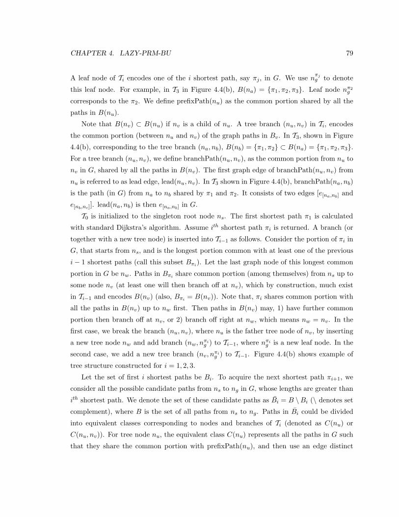
CHAPTER 4. LAZY-PRM-BU 79
A leaf node of Ti encodes one of the i shortest path, say πj, in G. We use nπjg to denote
this leaf node. For example, in T3 in Figure 4.4(b), B(na) = {π1, π2, π3}. Leaf node nπ2g
corresponds to the π2. We define prefixPath(nu) as the common portion shared by all the
paths in B(nu).
Note that B(nv) ⊂ B(nu) if nv is a child of nu. A tree branch (nu, nv) in Ti, encodes
the common portion (between nu and nv) of the graph paths in Bv. In T3, shown in Figure
4.4(b), corresponding to the tree branch (na, nb), B(nb) = {π1, π2} ⊂ B(na) = {π1, π2, π3}.For a tree branch (nu, nv), we define branchPath(nu, nv), as the common portion from nu to
nv in G, shared by all the paths in B(nv). The first graph edge of branchPath(nu, nv) from
nu is referred to as lead edge, lead(nu, nv). In T3 shown in Figure 4.4(b), branchPath(na, nb)
is the path (in G) from na to nb shared by π1 and π2. It consists of two edges [e[na,nb] and
e[nb,nc]]. lead(na, nb) is then e[na,nb] in G.
T0 is initialized to the singleton root node ns. The first shortest path π1 is calculated
with standard Dijkstra’s algorithm. Assume ith shortest path πi is returned. A branch (or
together with a new tree node) is inserted into Ti−1 as follows. Consider the portion of πi in
G, that starts from ns, and is the longest portion common with at least one of the previous
i − 1 shortest paths (call this subset Bπi). Let the last graph node of this longest common
portion in G be nw. Paths in Bπishare common portion (among themselves) from ns up to
some node nv (at least one will then branch off at nv), which by construction, much exist
in Ti−1 and encodes B(nv) (also, Bπi= B(nv)). Note that, πi shares common portion with
all the paths in B(nv) up to nw first. Then paths in B(nv) may, 1) have further common
portion then branch off at nv, or 2) branch off right at nw, which means nw = nv. In the
first case, we break the branch (nu, nv), where nu is the father tree node of nv, by inserting
a new tree node nw and add branch (nw, nπig ) to Ti−1, where nπi
g is a new leaf node. In the
second case, we add a new tree branch (nv, nπig ) to Ti−1. Figure 4.4(b) shows example of
tree structure constructed for i = 1, 2, 3.
Let the set of first i shortest paths be Bi. To acquire the next shortest path πi+1, we
consider all the possible candidate paths from ns to ng in G, whose lengths are greater than
ith shortest path. We denote the set of these candidate paths as Bi = B \Bi (\ denotes set
complement), where B is the set of all paths from ns to ng. Paths in Bi could be divided
into equivalent classes corresponding to nodes and branches of Ti (denoted as C(nu) or
C(nu, nv)). For tree node nu, the equivalent class C(nu) represents all the paths in G such
that they share the common portion with prefixPath(nu), and then use an edge distinct

CHAPTER 4. LAZY-PRM-BU 80
na
π2
nd
π3ne
ns
ng
π1
π2
π3
π1π3
nf
nh
nc
nb
π2 π1
ns
nsns
[1] [2]
[1, 2]
nπ1g n
π2g
ns
nπ1g n
π2gn
π3g
[1][3]
[1, 2, 3]
[2]
na[1, 2]
nπ1g
nb
nb
T0 T1
T2 T3
(a) shortest paths over the graph (b) Updating of the associated branch structure
Figure 4.4: Building of the branching structure of the shortest path tree T3.
from any of the lead edges lead(nu, nvj), j = 1, · · · , α, where nvj is the jth child of nu in Ti.
For tree branch (nu, nv), the equivalent class C(nu, nv) denotes all the paths in G, which
diverge from prefixPath(nv) somewhere strictly between nu and nv. [29] showed that,
[∪nu∈TiC(nu)]
⋃
[∪(nv,nw)∈TiC(nv, nw)] = Bi (4.6)
The shortest path for each equivalent class is calculated (line-8, Algorithm 12) and these
paths are stored in a heap. In each iteration, the shortest path in the heap is popped out,
and is the next shortest path. The tree structure Ti is updated (line-6, Algorithm 12).
4.2.4 Calculating the Shortest Path in an Equivalent Class
The key step in the above k-shortest path algorithm is to compute the shortest path in an
equivalent class, which can be formulated as a replacement paths problem. The description
in this subsection is roughly based on [29]. We briefly describe the corresponding algorithm
below for completeness.
We first introduce the replacement paths problem. Let π∗ be the shortest path from ns
to ng, where π∗ = {n1, n2, · · · , nl − 1, nl}, such that n1 = ns and nl = ng. We want to
compute the shortest path from ns to ng, that does not include the edge (ni, ni+1, for each
i ∈ 1, 2 · · · , l − 1. We call this the best replacement path for (ni, ni+1).

CHAPTER 4. LAZY-PRM-BU 81
Algorithm 12: k-shortest path algorithm
begin1
Initialize T0 to ns; H = ∅2
Calculate the 1st shortest path π1, insert π1 into heap H3
. for i=1; i < k; i++ do4
Extract the next shortest path πi from H.5
Ti = updateTreeStructure(π,Ti−1)6
for Each new node and branch in Ti do7
Apply replacement paths algorithm to compute the shortest path π, from8
ns to ng, in the equivalent class, corresponding to the new node (orbranch) .Insert π into heap H9
end10
notation: H - a heap.
The subroutine, which determines all the replacement paths, takes O(|E| + |V |log|V |)time, and can be used to compute the shortest path in an equivalent class as follows.
Consider an equivalent class C(nu, nv) with a branch (nu, nv) in T . Let nb be the graph
node next to nu, along with the branchPath(nu, nv) in the graph G. We determine the
shortest path in C(nu, nv)), using the replacement paths problem in a subgraph H of G. H
is acquired by deleting from G all the nodes on the prefixPath(nu). In H, we can tell that
the shortest path from nb to ng (denoted as π∗H) coincides with the branchPath(nu, nv) up
through nv. Let [nb = n1, n2, · · · , nl = nv] be the sub-path of π∗H (from nb to nv). We solve
the replacement paths problem in H, from nb to ng for all the edges (ni, ni+1), i = 1, · · · , l.
The shortest of these replacement paths, appended to the prefixPath(nu), is the shortest
path in the equivalent class C(nu, nv).
The shortest path in the equivalent class C(nu) for a tree node in T is acquired as
follows. We obtain a graph H by deleting from G all the vertices in the prefixPath(nu)
except nu, plus all the lead edges that leave from nu. We compute the shortest path from
nu to ng in H, then append it to the prefixPath(nu).
4.2.5 Lazy-PRM-BU
Our lazy-PRM-BU algorithm (Algorithm 13) works as follows. We maintain a label tree,
using a labeling algorithm that creates labels but only for graph nodes along the paths being
verified (line-11). Given a path to verify, the labeling algorithm starts labeling nodes from

CHAPTER 4. LAZY-PRM-BU 82
the start node ns by extending labels along the path. If the generated label at a graph node
is determined as efficient (as explained in labeling algorithm in Section 4.1.3), it is stored
and is added as a child of the tree node, from which this new efficient label was extended.
Then the next node in the path is considered, and procedure is repeated. If an extended
label is determined as in-efficient, the path verification step stops. The path is deemed
invalid, and the next shortest path is considered for verification.
Assume that i paths have been verified and failed. To get the next path for verification,
we modify the k-shortest path algorithm. Let us focus on the equivalent classes correspond-
ing to the nodes and branches of the branching structure Ti. The key is to identify an
equivalent class such that none of the paths in it will be the solution path. This entire class
can be eliminated from consideration for next shortest path, hence leading to efficiency.
Given Ti, consider an equivalent class C(nu, nv) (or C(nu)), which is a subset of all
candidates paths in Bi. Note that, starting from ns, all candidate paths in C(nu, nv) (or
C(nu)) share common portion with prefixPath(nu) up to nu. A key insight is that if the
label that corresponds to prefixPath(nu) is not efficient, none of the candidate paths in
the entire equivalent class will be the optimal solution path and the entire class can be
eliminated from further consideration (line-17, Algorithm 13). We refer to these equivalent
classes as invalid.
To tell whether an equivalent class is valid or not (line-17), we check the label tree
(created in line-11). For the equivalent class C(nu, nv) (or C(nu)) that corresponds to a
tree branch (nu, nv) (or a node nu) of Ti, prefixPath(nu) is a portion of at least one of
previous i shortest paths in G, which has been verified. The verification information has
been stored as labels in the label tree. For equivalent class (C(nu, nv) or C(nu)), we track
along the label tree from the root node along the prefixPath(nu). If we encounter a label tree
node (the leaf node included) that contains node nu, the equivalent class is valid. Otherwise
the equivalent class is invalid.
It is straightforward to show that the proposed method mentioned above returns the
shortest path that satisfies the constraint on likelihood of being collision-free if one exists,
and returns failure otherwise. Based on Equation 4.6, any path in G other than those
encoded in Ti belongs to at least one equivalent class. We excludes those invalid equivalent
classes (denoted as Biinvalid
), which only contains paths that can not be the solution path,
from Bi. Then, it is the shortest path in Bi \ Biinvalid
that is our returned path, and is
verified at each iteration. Obviously, the first valid path for verification will be the shortest

CHAPTER 4. LAZY-PRM-BU 83
Algorithm 13: Lazy-PRM-BU: Lazy PRM algorithm with base pose uncertainty
begin1
R = BuildInitRoadMap()2
Initialize T0 to ns; H = ∅3
Calculate the 1st shortest path π1, insert π1 into heap H.4
InitLabeling(), i=1.5
while T imeUp() do6
Extract the shortest path from the heap, which will be the next shortest path7
πi.if πi == NULL then8
EnhanceRoadMap();9
else10
if verifyPath(πi) then11
return πi;12
else13
Extract the next shortest path πi from H.14
Ti = updateTreeStructure(π,Ti−1)15
for Each new node and branch in Ti do16
if the corresponding equivalent class is valid then17
Apply path replacement algorithm to compute the shortest18
path π, from ns to ng, in the equivalent class, corresponding tothe new node (or branch).Insert π into heap H19
i++20
end21
one that satisfies the constraint on collision probability.
4.2.6 Roadmap Construction and Node Enhancement
We ensure that all the nodes in the constructed roadmap are S-nodes, which can be easily
achieved as described in Section 4.1.1. If our lazy query reports a failure, we enhance the
roadmap by inserting more S-Nodes and connecting them to the current roadmap. All the
data structure for k shortest path calculation, such as the branch tree structure Ti as well
as the queue etc., are initialized again. But the label tree can be reused, because all the
labels in current the label tree are efficient, and they do not need to be created again.

CHAPTER 4. LAZY-PRM-BU 84
4.2.7 Detecting an N-edge
In the path verification step, if we encounter an N-edge, there are two alternations: (I) keep
searching for the next shortest paths using current graph, (II) remove the edge from the
graph, delete the old shortest path tree and build a new one from start for the new graph,
which is similar to the original Lazy-PRM . However, if we already have a large shortest
path tree, removing an N-edge from the graph and rebuilding the shortest path branch tree
structure Ti may not be efficient 1.
In our implementation, we found a practical solution that works well in our experiments.
If the ratio between the number of the nodes in Ti and the number of the N-edges in the
roadmap is smaller than a threshold (we use 50 throughout this work) we will delete the N-
edge from the graph and rebuild the shortest path tree. Otherwise, we keep on the searching
using the same graph and the current shortest path tree.
4.2.8 Path Verification from Both Directions
As suggested in [28], checking end nodes (nodes close to start and goal) of the path benefits
the overall searching performance. In our implementation, we root two label trees from both
start and goal, and verify paths from both directions. Each time we detect an N-edge and
rebuild the shortest path tree, we will switch the direction (from the start node to the goal
or from the goal node to the start node) for the path verification step, and update the label
trees correspondingly.
4.3 Simulations
We have run preliminary tests of PRM-BU and Lazy-PRM-BU in our simulated test-bed
(introduced in chapter of introduction). We use the MobileSim [79] program as our mobile
robot simulator to simulate a PowerBotTM
[79], with a size of about 80cm by 65cm. A
simulated range sensor, with sensing range of 4.0 meters (approximately the same range
as the Hokuyo range sensor), is mounted on the mobile base and points to the front. The
simulated manipulator on-board has three degrees of freedom, and each link is 90cm long.
We simulate an “inspection” task, i.e., the desired goal configuration is as if the arm (say,
1Note that after an N-edge is removed from the graph G, it might be possible to acquire the branchstructure Ti efficiently from the old branch structure incrementally without rebuilding the whole structurefrom scratch. See Chapter 6 for future work.

CHAPTER 4. LAZY-PRM-BU 85
with a camera mounted on the end-effector) was inspecting an area behind the obstacles in
Figure 4.5 (b). We run our simulation under Linux on an Intel Core-2 due 3.0Ghz computer
with 4GB RAM.
We compare the lazy-PRM-BU algorithm with the PRM-BU in four tasks as shown
in Figure 4.5, where sub-figures on the left show paths planned with PRM-BU with base
uncertainty, and sub-figures on the right show paths planned with classic PRM with no
uncertainty taken into account and with the base pose at the most weighted particle. We
assume the robot is in the middle of an exploration task. The black regions are sensed
obstacles, gray regions are unknown and white regions are free. Figure 4.5 (a) and (b) show
the manipulator moving from an unfolded configuration to another unfolded goal configu-
ration. Figure 4.5 (c) and (d) show the manipulator moving from a folded configuration to
an unfolded goal configuration.
We simulate the base uncertainty as follows. We use the true position of the base as the
mean and apply a Gaussian pdf to generate 30 particles (a number that is commonly used
in particle based localization algorithms [7]). The covariance matrix of the Gaussian pdf is
diagonal with the diagonal element values being (0.12m,0.12m,3o) for LARGE uncertainty
and (0.07m,0.07m,1o) for SMALL uncertainty, in x,y and θ dimension, respectively.
To acquire a goal configuration, the most weighted particle used as the base pose, and
a sampling based inverse kinematics technique [80] is used to generate a configuration,
whose end effector is pointed to the designated end effector position. Although we could
set a threshold for probability of being collision free for the goal configuration, we require
(conservatively) this manipulator goal configuration is free for all the base particles. This
generated configuration is used as the goal configuration.
In all our simulations, we set the threshold δ for the collision-free probability of a valid
path as 0.8. For raodmap construction step, the initial roadmap has 500 nodes, and is
enhanced with 50 nodes each time. We ran the planner(s) 30 times for each problem. Note
that for each task, we also set a time limit, which is 1000, and 1500 seconds for SMALL
and LARGE uncertainty, respectively. The results are listed in Table 4.1 to 4.3.
Our first observation is how the base uncertainty affects the planned path. In Figure 4.5,
the sub-figures on the left illustrate some paths planned with the base uncertainty taken into
consideration (the uncertainty size is LARGE), while sub-figures on the right illustrate paths
planned with the true base pose (without any uncertainty) using classic PRM. Note that
paths planned with classic PRM are, at times, closer to the obstacles, as in Figure 4.5 (b).

CHAPTER 4. LAZY-PRM-BU 86
(a) Problem A
(b) Problem B
(c) Problem C
(d) Problem D
Figure 4.5: Four different start/goal problems. Left: paths planned with PRM-BU withbase uncertainty (LARGE). Right: paths planned with classic PRM with no uncertaintytaken into account and with the base pose at the most weighted particle.

CHAPTER 4. LAZY-PRM-BU 87
Unc. G. size Av. Time Av. En. Searching Av.|E| |V | Total Cons. Search Coll. Av. Paths Inv-Cls.
ASL
6698 5026668 502
18.9 2.5 2.1 14.324.4 2.0 6.5 15.8
00
118 39544 575
BSL
6838 5077678 527
13.8 2.5 1.7 9.626.5 1.5 12.7 12.3
0.10.5
97 371229 1461
CSL
6678 5036801 507
51.4 2.1 22.2 27.188.6 2.8 55.1 31.7
0.030.1
1885 24594178 5816
DSL
6838 5076767 505
97.7 3.0 49.6 45.2129.5 2.7 76.4 50.4
0.070.23
3283 46035478 7300
Table 4.1: Results for Lazy-PRM-BU with pruning invalid equivalent classes.
Unc. G. size Av. Time Av. En. Searching Av.|E| |V | Total Cons. Search Coll. Av. Paths Inv-Cls.
ASL
6632 5026690 502
325 322 2.9 320318 315 3.2 313
00
1.9 1.16.9 5.4
BSL
7301 5207749 528
323 321 2.5 319326 321 4.7 320
0.370.53
3 179 87
CSL
6737 5046781 508
327 324 3.3 322324 321 3.1 319
0.030.13
3 34 4
DSL
6697 5026791 507
320 315 4.6 318323 315 8.4 312
00.1
30 39149 211
Table 4.2: Results for PRM-BU.
Unc. PRM-BU Lazy-PRM-BU♯Edges ♯Total ♯Edges ♯Total
ASL
6632 45183786690 4534507
139 203246179 252654
BSL
7301 49109117749 5277889
79 153531134 190784
CSL
6737 45917206781 4674345
232 319204321 445487
DSL
6697 45762016791 4566823
395 533990461 631613
Table 4.3: Number of collision checking for Lazy-PRM-BU and PRM-BU.

CHAPTER 4. LAZY-PRM-BU 88
700
800
Env C
Sec.
500
600
Env.C
300
400
500
PRM
200
300
Lazy P
0
100 Lazy-P
0
Uncertainty size: SMALL
Env. D
M-BU
PRM BUPRM-BU
30
(a) SMALL uncertainty1400
Sec.
1000
1200
Env D
800
Env.CEnv. D
400
600
PRM-
0
200
0
Uncertainty size: LARGE
Env. D
-BU
Lazy-PRM-BU
30
(b) LARGE uncertainty
Figure 4.6: Running time for problems A to D for all the 30 runs.

CHAPTER 4. LAZY-PRM-BU 89
Unc. G. size Av. Time Av. En. Searching Av.|E| |V | Total Cons. Search Coll. Av. Paths Inv-Cls.
ASL
7186 5207278 505
49.2 2.7 38.5 8.1156 2.4 140 13.7
0.40.5
984 05533 0
BSL
6723 5026689 502
89.8 2.7 71.9 15.2107 2.2 89.1 15.9
00
2313 03407 0
CSL
6630 5026824 507
95.4 3.3 65.2 26.9185 2.3 154 28.0
00.1
2215 05349 0
DSL
6996 5127656 527
185 3.3 149 32.2543 2.9 509 30.8
0.20.5
4340 014586 0
Table 4.4: Results for Lazy-PRM-BU without pruning invalid equivalent classes.
A B C DS L S L S L S L
♯F w. pr. 0 0 0 0 0 0 0 0w.t. pr. 1 1 2 2 2 3 4 10
WT w. pr. 25 145 31 137 589 311 538 903(Sec.) w.t. pr. > 1000 > 1500 > 1000 > 1500 > 1000 > 1500 > 1000 > 1500
Table 4.5: The number of failure times (FT) and worst case time (WT) for Lazy-PRM-BU(30 runs) with (w. pr.) and without (w.t. pr.) pruning invalid equivalent classes. Timelimit is 1000 and 1500 seconds for SMALL and LARGE uncertainty, respectively.
Clearly, the paths planned with the base uncertainty tend to be consistently safer. For the
four start/goal problems in Figure 4.5, the probability of being collision-free for the paths
planned with PRM-BU are 0.960, 0.985, 0.808 and 0.815, respectively. We also calculated
this probability for the paths planned using classic PRM and they were, 0.760, 0.303, 0.740
and 0.825, respectively. This clearly illustrates the desirability of using PRM-BU.
Table 4.1, 4.2 and 4.3 show the efficiency of our proposed Lazy-PRM-BU v.s. the PRM-
BU. In these tables, “Unc.” is the size of the base uncertainty, which is marked as “S”
and “L”, standing for SMALL and LARGE uncertainty as mentioned before. The second
column “G. size Av.” is the average graph size, including number of edges (|E|) and nodes
|V |, used to find a solution. The third column, “Time Av.” records the average time spent
to find the path (Total), to construct the roadmap (Cons.), to search the graph (sear.),
and to check collisions (col.). The average number of times the roadmap is enhanced is
recorded in the fourth column. In the fifth column, i.e. “Searching Av.” shows the number
of shortest paths verified before the solution path is found (“paths”), and the number of the
equivalent classes that are invalid (“Iv-Cls”). Finally, the average number of edges being
checked for collision, and the average total number calls of the collision checker are listed in
Table 4.3.

CHAPTER 4. LAZY-PRM-BU 90
Our Lazy-PRM-BU, as shown in Table 4.1, is capable of solving the single query ef-
ficiently. Lazy-PRM-BU, saves significant time on collision checking, but does spend, as
expected, bit more time on the k-shortest path calculation. Please note that in our envi-
ronment setup, the cost of a collision check is quite small (checking intersections of simple
polygons in the planar). In real scenarios (3-D case), collision checking cost is high, partic-
ularly if the geometry of the robot and environment is complex. In such cases we expect
significantly more saving in the overall time for Lazy-PRM-BU for single query problem, as
compared to PRM-BU.
We also observe, as expected, that increasing the base uncertainty tends to make it
harder to find a path. For example, in problem shown in Figure 4.5 (a) the number of paths
needed to be verified increases almost 10 times.
Our lazy-PRM-BU is efficient because it prunes all invalid equivalent classes. We also
ran it without pruning the invalid classes, for each of these four tasks, and show the results
in Table 4.4. Clearly, the number of paths to be verified increases dramatically (up to by an
order of 10) in these tasks. Table 4.3 shows the number of times lazy-PRM-BU, with and
without pruning those in-valid classes, runs over the time limit, as well as the worst case
run time. Our Lazy-PRM-BU clearly benefits from pruning those invalid equivalent classes.
In Figure 4.6, we also plot the time spent on each problem for all the 30 runs for Lazy-
PRM-BU and PRM-BU. In problem C and D, we did observe that the worst cases time
spent for the Lazy-PRM-BU (those high peaks pointed by arrows) is even longer than the
average of time for PRM-BU. But this happens only in a very occasionally manner (2-3
times out of 30 runs), and the worst time is still with in a reasonable range.
4.4 A Motion Planner for the Mobile Manipulator System in
an Inspection Task
In this section, we briefly demonstrate an integrated motion planner for the mobile manip-
ulator that combines, in a decoupled manner, RRT-SLAM for mobile base with Lazy-PRM-
BU in a specific environment inspection task, which originally motivated this research. We
assume an end effector goal position is given in advance, and the manipulator is initially in
a fixed folded configuration.
As mentioned earlier, our planner decouples the base planning with the manipulator
planning similar to [1, 19]. The planner will first invoke RRT-SLAM to move the base

CHAPTER 4. LAZY-PRM-BU 91
close to the end effector position, such that I) the localization uncertainty of the node is
smaller than a threshold ubound (the localization uncertainty is measured by the area of the
bounding box for the base pose particles. We use 0.1m2 in our simulations below), II) the
goal end effector position is within the reachable workspace of the manipulator. A coarse
approximation is sufficient here, i.e., in our case, the base position must be within a distance
lmax (lmax =∑
li, li is the length of the ith link) of the end-effector position.
Then, the planner uses Lazy-PRM-BU to find a path for the manipulator with the base
pose uncertainty given by the latest tree node. The goal configuration for Lazy-PRM-BU
is acquired with inverse kinematic calculation in the same way as what has been described
for problems in Section 4.3.
This planner is implemented and tested in our simulated test-bed, as given in Figure
4.7. After a portion of the environment is explored, an inspection point (shown as a black
square in Figure 4.7 (a)) is to be reached by the arm end-effector. This point is hard for
the mobile base to access by itself. The threshold for the collision-free probability for the
base motion and the manipulator motion are set as 0.85 and 0.8, respectively. A sequence
of decomposed planned motions for the mobile base and the manipulator in this inspection
task are illustrated in Figure 4.7 (b) and (c), respectively. In Figure 4.7 (b) the probability
of the planned base path being free is 1. In Figure 4.7 (c), the probability of the planned
manipulator path being free is 0.943.

CHAPTER 4. LAZY-PRM-BU 92
(a)
(b)
(c)
Figure 4.7: The robot is given an end effector position as goal shown in sub-figure (a),which is a partially explored environment. The end effector position is marked by the blacksquare. In (b), the mobile base first moves close to the designated end effector position(path planned with RRT-SLAM), and then execute the manipulator path returned by theLazy-PRM-BU, with the base being stationary (c).

Chapter 5
DTC: Delaunay Triangulation
Inspired Adaptive k Nearest
Neighbor Roadmap Connection
Technique
In this chapter, we revisit one of the key issues, i.e., node connection, in the probabilistic
roadmap motion planner (PRM) framework, which is applied in Lazy-PRM-BU. We propose
a new neighborhood selection strategy based on certain empirically observed properties of
the Delaunay triangulation of a uniformly distributed random point set. This allows a
node in the network to have neighbors that are close to itself in the sense of the Delaunay
Neighborhood.
We first review the Delaunay triangulation, a basic concept in computational geometry
[81].
5.1 Delaunay Triangulation Review
Given a set S of n distinct points in Rd, the Delaunay triangulation is the geometric dual
of the Voronoi diagram. The Voronoi diagram of a point set S is the partition of Rd into
n polyhedral regions V (s), s ∈ S. Each region V (s) is a Voronoi cell of s, and is defined as
93
CHAPTER 5. DTC 94
the set of points in Rd which are closer to s than any other points in S:
V (s) = (r ∈ Rd | ρ(r, s) ≤ ρ(r, s′
),∀s′ ∈ (S − s))
where ρ(.) is a distance function.
The set of all Voronoi cells and their faces form a cell complex. The vertices of this
complex are called Voronoi vertices. For each vertex v ∈ Rd, the nearest neighbor set
(denoted as nb(S, v)) of v in S is the set of points s ∈ (S − v) which are closest to v.
The convex hull conv(nb(S, v)) of the nearest neighbor set of a Voronoi vertex v in S is
called the Delaunay cell of v. The Delaunay triangulation of S is a partition of the convex
hull of S into Delaunay cells of Voronoi vertices together with their faces. The Delaunay
triangulation consists of a set of triangles in 2-dimensional space (see Figure 5.1), and an
aggregation of disjoint, irregular tetrahedra in 3-dimensional space, assuming that the input
points are non-degenerate. An example of a Delaunay triangulation and Voronoi diagram
of a point set in [0, 1]2, in 2-dimensional space is shown in Figure 5.1. Throughout this
chapter, we use Euclidean metric for Delaunay triangulation calculation.
5.2 PRM Sample Connection Strategy Review
Of main interest here is the Nearest Neighborhood Connection (NNC) strategy used in most
PRM algorithms. To determine the neighbor nodes for a given node nc (the ones the node
is connected to via a collision-free edge), a candidate neighborhood set Snc based purely on
the Euclidean metric is selected. In [26], a threshold Maxdist is used to bound the set of Snc
to be the samples located inside a ball that is centered at nc and has a radius of Maxdist .
Another constant MaxNumNeighbors bounds the size of the set Snc and guarantees that
the ratio between the number of the edges and nodes is approximately fixed. In [26] and
[28], those numbers are chosen experimentally, MaxNumNeighbors is typically of order of
30 when the dimension is 6. Maxdist is selected such that the number of the initial samples
inside a ball of radius of Maxdist is approximately equal to MaxNumNeighbors .
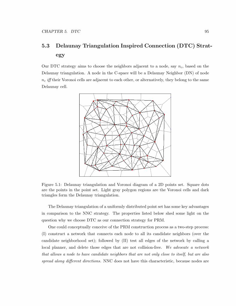
CHAPTER 5. DTC 95
5.3 Delaunay Triangulation Inspired Connection (DTC) Strat-
egy
Our DTC strategy aims to choose the neighbors adjacent to a node, say nc, based on the
Delaunay triangulation. A node in the C-space will be a Delaunay Neighbor (DN) of node
nc iff their Voronoi cells are adjacent to each other, or alternatively, they belong to the same
Delaunay cell.
Figure 5.1: Delaunay triangulation and Voronoi diagram of a 2D points set. Square dotsare the points in the point set. Light gray polygon regions are the Voronoi cells and darktriangles form the Delaunay triangulation.
The Delaunay triangulation of a uniformly distributed point set has some key advantages
in comparison to the NNC strategy. The properties listed below shed some light on the
question why we choose DTC as our connection strategy for PRM.
One could conceptually conceive of the PRM construction process as a two-step process:
(I) construct a network that connects each node to all its candidate neighbors (over the
candidate neighborhood set); followed by (II) test all edges of the network by calling a
local planner, and delete those edges that are not collision-free. We advocate a network
that allows a node to have candidate neighbors that are not only close to itself, but are also
spread along different directions. NNC does not have this characteristic, because nodes are

CHAPTER 5. DTC 96
connected based only on the distance between them. Instead, the Delaunay triangulation
network is constructed based not only on “distance” but also on “direction” information.
Consider a simple intuitive scenario as shown in Figure 5.2. In the left figure, if node B
has some neighbors approximately along a particular direction, say−−→BC, nodes further away
along the same direction, e.g., C, will not be direct neighbors of B. But if B does not have
many neighbors approximately along a direction, say−−→BA, nodes that are even though sort
of far away from B, e.g., A, still will be connected to B so long as they are “close neighbor
in that direction”. However, as shown in the right figure, as A is moved further along the
direction−−→BA, it will get disconnected from node B because it is too far away from B. Hence
the Delaunay neighborhood selection for a uniformly distributed point set keeps a balance
between “distance” and “direction”.
Figure 5.2: Delaunay triangulation inherently uses both distance and direction information.See text for explanation.
5.3.1 Constructing a Delaunay Triangulation Neighborhood
There exist efficient algorithms for computing the Delaunay triangulation and the Voronoi
diagram for lower dimensions, specifically O(N log N) (N is the number of the set points)
algorithms in 2D, and almost O(N log N) algorithms in 3D [81]. Explicit calculation of
Delaunay triangulation will output all the Delaunay cells and a data structure that facilitates
visiting all the cells. When the dimension is high, it has exponential complexity (there exist
an incremental O(N ⌈ d2⌉) algorithm [82]) with respect to the dimensionality, hence intractable

CHAPTER 5. DTC 97
[83]. However, we do not need to build an explicit Delaunay triangulation. We are only
interested in constructing a Delaunay network, inside which two nodes will be connected
by an edge when they belong to the same Delaunay Cell, i.e., they are Delaunay Neighbors
(DN). The problem of deciding if two nodes are Delaunay Neighbors or not, can be posed as
a linear programming (LP) problem, and the description of the corresponding LP problem
below is roughly based on [84].
The Voronoi diagram of a set S of N points in Rd is the projection of the following
(d + 1) polyhedron to Rd space of the first d components:
P = {x ∈ Rd+1|d
∑
j=1
s2j −
d∑
j=1
2sjxj + xd+1 ≥ 0,∀ s ∈ S}
It can be relisted as:
P = {x ∈ Rd+1|b − Ax ≥ 0},
where A is an N × (d + 1) matrix and b is an N -vector. Now, we formulate the following
LP for any distinct i, j = 1, 2, . . . , n
minimize f(x) := bj − Ajx
subject to b′ − Ax ≥ 0
bi − Aix ≤ 0,
(5.1)
where Aj stands for the jth row of A and vector b′
is equal to b except that the jth component
of b′
(denoted by b′
j) is equal to bj + 1 (b′
j = bj + 1).
The Voronoi cell of points i and j are adjacent, i.e, i and j will be Delaunay Neighbors,
if and only if the objective value f(x) is negative at an optimal solution.
So we can decide whether two nodes are Delaunay Neighbors by solving a LP problem
which has N + 1 constraints and can be solved in polynomial time in N . Unfortunately,
it would involve solving O(N2) LP problems to construct the whole Delaunay network. It
would be computationally expensive, to build the Delaunay network exactly because each
LP problem includes N + 1 constraints and every constraint has in turn d variables for d
dimensional space.
We alternatively suggest an efficient approach that will build a network that is “similar”
to Delaunay network. The motivation behind our approach comes from some empirically

CHAPTER 5. DTC 98
observed “statistical” properties of Delaunay neighbors.
Let S be a set of n points that is uniformly distributed inside a unit cube in a d-
dimensional space. Let nc be a node in S that is closest to the center of the cube. When
| S |= N is large enough, a key question arises:
Question 1: How are the Delaunay Neighbors (DNs) of nc distributed?
We answer the question by conducting an experiment below.
Experiment A: We rank all the nodes in S′ = S\nc by their distance to node nc and
we denote the distance ranking of a node, say ni ∈ S′, as ki. Given a ki, we empirically
determine the probability that node ni is a DN of nc.
Since we can easily tell whether two nodes are DNs by solving an LP problem, it is
easy to conduct the experiment by generating a uniformly distributed random point set S
several times and then computing the probability for a given ki. We varied cardinality of
the set S in a range from 1000 to 3000 with an increment of 100. We repeated the testing
100 times for every sample size, and estimated the probability by computing the average
over all sample sizes.
Figure 5.3: Probability for a node of ranking ki to be DN of node nc, in 6-dimensional space
The result of Experiment A is presented in Figure 5.3. It clearly shows that for a given
dimensionality, the higher is the ranking of a node (i.e., the closer it is to node nc), the higher
is the probability that this node is a DN of nc and vice versa. There is also a boundary like
area, (let us denote the two edges of this boundary with k−b and k+
b , respectively) such that
we can tell, with a high degree of certainty that a node with a ranking outside this area is a

CHAPTER 5. DTC 99
DN of nc or not. In Figure 5.3 k−b and k+
b are around 100 and 240, respectively. The width
of the band [k−b , k+
b ] is always small compared to the size of set S. It should be pointed out
that the distribution shown in Figure 5.3 is not sensitive to the size of the sample set S so
long as the size of S is large enough. Note that learning precise value of k−b and k+
b is not
important here, since we only build a network that is “similar” to Delaunay network (see
Algorithm 15 later for detail). We now can choose a number kb inside this band [k−b , k+
b ]
as a boundary (see STEP 1 in Algorithm 14 for detail). Obviously kb can be used as an
estimate of the expected number of DNs of nc. We choose kb as follows. From the plot as
shown in Figure 5.3, traversing from left to right, kb will be the ranking number, where the
first time the probability falls below a threshold (we choose 0.4 in all our simulations).
Question 2: For large enough S, how does kb vary with respect to dimension?
Figure 5.4: Selection of kb for each dimension from 2 to 10
We repeated the above experiment for point sets in different dimensions, ranging from
2 to 10. Figure 5.4 shows the empirical variation of kb (determined by applying STEP 1,
Algorithm 14) for different dimension d, when the set size is large enough. The dependence
of kb on d seems to be of exponential nature1.
Indeed, it is possible to find a ball centered at nc such that the expected number of DN
nodes inside the ball is kb. The radius of the ball corresponds to the expected value of actual
distance between nc and its kthb closest neighbor. We denote the radius as Rd. Figure 5.5
shows the empirically determined minimal, average and maximal radii of ball that contains
1Based on this empirical data, if we were to have a guess, kb ≃ O(f(d) ∗ 2d), where f(d) is larger than 1,and increases slowly with d.

CHAPTER 5. DTC 100
exactly kthb neighbors, for different sample sizes, with 100 runs for each sample size, in 2D,
4D and 6D. The corresponding value for kb are 12, 56 and 150, respectively. In the plot,
the y-axis represents the radius that is normalized as Rd/√
d, where√
d is the diagonal of
length of a unit cube in dimension d.
5.3.2 Delaunay Triangulation Inspired Adaptive Roadmap Connection
(DTC)
Algorithm 14: Calculating Rd for given dimension d:
begin1
STEP 1: Calculating kb2
Select an arbitrary number k (approximately around 2d is a good start). Here k3
represents the ranking of distance from nc to all the other samples.while 1 do4
for counter = 0 to 100 do5
Put n (We set n = 3000) random uniform samples inside a cube [0, 1]d .6
Pick up a sample closest to the center of the cube [0, 1]d, and denote it as7
nc.Calculate the distance from nc to all the other samples, and select the kth
8
closest neighbor of nc. Denote it as nk.Test whether nk and nc are Delaunay Neighbors by solving the LP9
problem in Equation 5.1.
Calculate the fraction of instances that nk and nc are Delaunay Neighbors.10
This is an estimation of probability (denoted as Pk) that nk is a DN of nc .if Pk is less than a threshold (we choose 0.4 in all the simulations) then11
set kb = k.12
break13
else14
k = k + 1.15
STEP 2: Calculating Rd16
Having determined kb, generate another uniform sample set (let the size of sets17
start from 100) 100 times and take the average of the distance value, denote asRd, between nc and nkb
, i.e., the sample whose distance ranking to nc is kb.Increase the number of uniform samples and repeat step 8 to construct a lookup18
table T that stores Rd for different sample sizes.end19
In Algorithm 14, we give the detailed algorithm to calculate kd for different d (STEP

CHAPTER 5. DTC 101
Figure 5.5: Relationship between the number of uniform nodes and radius selection (theaverage value) in 2, 4 and 6-dimensional spaces.

CHAPTER 5. DTC 102
1), and Rd for different sample sizes for a given dimension d (STEP 2). The relationship
shown in Figure 5.5, i.e., the normalized radius Rd (we used the average value) for different
sample sizes, can be stored in a lookup table T (line 13) for each dimension.
We now state our Delaunay triangulation inspired connection algorithm (Algorithm
15). For each node ni, we consider all the nodes whose distances to ni are less than Rd,
which is acquired from table T , as the candidate neighbors. But connecting ni with all
the candidate neighbors may lead the roadmap contains too many edges, especially when
dimension d is high, say above 6. We introduce the same parameter as standard PRM,
MaxNumNeighbors, which works as an upper-limit to the number of Delaunay neighbors.
However we randomly choose MaxNumNeighbor nodes among the candidate neighbor set
within radius Rd.
Algorithm 15: Delaunay triangulation Inspired Connection (DTC)
begin1
For a node ni, select the radius Rd from the lookup table T based on current2
number of uniform nodes.Store all the neighbors, whose distances to ni are less than Rd, in a list L.3
if the length of list L less than MaxNumNeighbors then4
connect the node ni with all the nodes in L.5
else6
randomly choose MaxNumNeighbors neighbors (exclude the nearest7
neighbor of ni) from the list L as the neighbors of ni.
end8
Typically, the number of nodes inside the radius will be around 100 when the dimension
is up to 6 or 7. Our strategy of randomly choosing neighbors among the candidates in a
list L (line 3, Algorithm 15) will permit some “long distance” neighbors and not simply k
closest neighbors, as is the case in NNC.
5.3.3 Node Enhancement
Our enhanced samples are generated in the same way as described in [26] but with some
corresponding modifications to the enhanced node connection step. We introduce a scalar
parameter α ≥ 1 and use αRd as the radius of neighborhood selection for the enhanced
nodes. This is based on the observation that inside narrow passages, the number of the
nodes is sparse, hence requiring a larger radius to include more nodes. In our simulations

CHAPTER 5. DTC 103
we choose α = 1.5.
5.4 Simulations
We now present some tests with DTC algorithm for 2D, 4D and 6D configuration spaces. We
choose the parameter MaxNumNeighbors as 8, 15 and 25, respectively. The planner has
been implemented within Motion Planning Kernel (MPK) Library [85] developed in RAMP
lab, SFU. All the simulations have been run on a 2.0GHz Pentium4 PC. The collision
detector used in all these examples is V-Collide library developed at University of North
Carolina [77].
We first tested our planner on a 2D rigid mobile robot. In environments A and B (see
Figure 5.6 left and right respectively), the robot needs to go through some narrow passages
to reach the goal. Environment C and D (Figure 5.7 left and right, respectively) depicts
solutions for two 4D planning problems and environment E (Figure 5.8) is a 6D planning
problem. Configurations in light color represent the start and goal, respectively. Dark
colored configurations are some intermediate configurations along the solution path. The
sample generation strategies in all our simulations are the same for both NNC and DTC.
Figure 5.6: Problems A (left) and B (right) – 2D rigid mobile robot
We performed 20 trials for each example. Table 5.4 shows the average time taken and
the average number of nodes used to solve each problem for NNC and DTC, respectively.
In our simulations the time spent on the node connection for NNC and DTC is very similar.

CHAPTER 5. DTC 104
Figure 5.7: Problems C (left) and D (right) – 4-link planar manipulator with fixed base.
Figure 5.8: Problem E – 6-link planar manipulator with fixed base.

CHAPTER 5. DTC 105
DTC shows obvious improvements in performance in terms of planning time. The variance
of the run time for the same problem is significantly lower for DTC. This supports our
assertion that DTC is a better connection strategy than NNC.
Pro. Connecter ♯Nodes Time(sec.) Time-Var
NNC 1023 85.6 2812A DTC 750 53.0 730
NNC 1038 64.4 1920B DTC 718 39.8 536
NNC 2183 665 543068C DTC 955 273 144571
NNC 270 155 7526D DTC 201 105 4870
NNC 2350 4298 10571372E DTC 1440 2857 2770558
Table 5.1: Simulation results for problems A, B, C, D and E.

Chapter 6
Conclusions and Future work
In this thesis, we studied two key motion planning sub-problems arising in exploration and
inspection tasks for a mobile manipulator, where the motion planner has to incorporate
robot localization and mapping uncertainties. The sub-problems correspond to I) motion of
the mobile base, considering both the localization and the mapping uncertainties, II) motion
of the manipulator only (with the mobile base being stationary), considering the base pose
uncertainty. We used particle based uncertainty representation, and stochastically formulate
the collision probability of a path. We used the collision probability as the travel cost. Our
planners return, a feasible (for mobile base) and an optimal (in terms of the path length)
path (for manipulator) path, subject to constraint that the probability of being collision
free is higher than a user define threshold.
We proposed RRT-SLAM to solve the first subproblem. It takes the sensor observations
into consideration, and combines RRT with a simulated particle based SLAM algorithm
(FastSLAM) to expand the tree in the UC-space. The collision probability along a planned
path is explicitly computed and is used to select a planned path. To improve efficiency of
RRT in the UC-space, we applied a fractal dimension (FD) based sequential data clustering
approach. A series of simulations show that the efficiency improvement of RRT-FD in
terms of planning time is up to 20% compared with standard RRT. The planners return a
feasible path, subject that the probability of being collision free is higher than a user defined
threshold.
We extended the probability roadmap approach to deal with the second subproblem, i.e.,
to plan motion of a manipulator system with base pose uncertainty, represented with a set of
particles. We formulated the path query as a constrained shortest path problem. We proved
106
CHAPTER 6. CONCLUSIONS AND FUTURE WORK 107
that the complexity of our path query is NP-hard w.r.t. the the number of the particles.
We solved the general query problem over a given roadmap, with a labeling algorithm, and
presented a novel lazy version of it. The lazy query technique, so called LAZY-PRM-BU,
aims to reduce the number of collision checking for fast single path queries. The key idea
to the efficiency improvement of our LAZY-PRM-BU approach is to combine the labeling
algorithm with the k-shortest path algorithm, such that a large number of invalid candidate
paths can be skipped from further consideration. Simulations show that our approach can
efficiently query the path over graphs with the size of up to 1000 nodes and 10000 edges. The
planners return an optimal path (in terms of the path length), subject that the probability
of being collision free is higher than a user defined threshold.
Finally, we studied the sample connection step in PRM’s roadmap construction, a key
step for all the roadmap based approaches. We proposed a new method of neighborhood
selection strategy based on certain empirically observed properties of Delaunay triangulation
of a uniformly distributed random point set. Our method allows a node in the network to
have neighbors that are close to itself in the sense of Delaunay Neighborhood. The Delaunay
triangulation connection (DTC) algorithm is easy to implement and we show the boost in
performance (20% to 50% running time) via a series of simulations.
6.1 Future Work
There is ample scope for future work here, both for algorithmic improvement, and for
several broad issues related to motion planning under uncertainties. First, we discuss the
algorithmic improvements.
We would like to extend RRT-SLAM, implemented on a mobile base in this research, to
the whole mobile manipulator system. The challenge would be the cost of collision checking
for the whole mobile manipulator system, and the significantly higher computational cost
introduced by the high dimensional C-space.
In Lazy-PRM-BU, when an N-edge is detected, we remove it from the graph. But the
shortest path tree has to be reconstructed in our implementation. It might be possible to
acquire the branch structure (refer to Chapter 4 for details) efficiently from the existing
branch structure incrementally without rebuilding the whole structure from scratch, hence
further improving the overall efficiency of the Lazy-PRM-BU.
With the base uncertainty in mind, PRM-BU and Lazy-PRM-BU focus mainly on the

CHAPTER 6. CONCLUSIONS AND FUTURE WORK 108
query phase. The sampling technique is the same as in the classic PRM, which uses uniform
samples generated in C-space. As shown in the classic PRM case, many biased roadmap
sample generation techniques tend to improve the PRM’s efficiency. It will be interesting to
study how these biased sampling techniques could be adapted to further improve efficiency
of PRM-BU (or Lazy-PRM-BU).
The DTC is investigated and tested in a model-based PRM framework. We have not
extended it to the case of PRM-BU. It will be interesting to see how this sample connection
strategy impacts the overall performance of PRM-BU. It is also worth investigating how
to extend DTC with other connection strategies, such as those using different metrics.
Weighted DTC may be one way to approach this. A good review of weighted metrics can
be found in [86].
We now discuss some practical and theoretical issues related to the planning under
uncertainty.
Throughout the work, we assume that a threshold for collision probability is given by
the user in advance (similarly, which is fixed in RRT-SLAM and PRM-BU). In practice, the
specific threshold would be experimentally determined by the user. We need further efforts
to determine the effects of the threshold on the planned path.
The eye sensor in our case is used for inspection task only, and is not used for unknown
environment exploration. How the eye sensor and the sensor on the base can be fused
together [13] for a more efficient exploration is an interesting problem.
In this work, we use a simulated planar mobile manipulator system as atest-bed. We
would like to extend our results on the actual mobile manipulator system 3D environments.
The Hokuyo type sensor can be mounted on a pan/tilt unit on the base for a 3D environment
modeling [63] or on the end effector for envrionment [11] and/or object modeling [13]. This
extension to the 3D case will bring further important practical issues, such as the model
representation, collision detector design, control of the actual robot system, view planning,
and higher degrees of freedom (6 dofs) for the manipulator to the fore.

Appendix A
System Implementation
A.1 The Simulated Mobile Manipulator Test-bed System
In this appendix, we detail the software structure of the motion planner and the simulated
mobile manipulator system that are used to demonstrate the proposed motion planning
techniques in this research. Our implementation of the system introduced here is mainly for
testing the proposed ideas. Similar architectures for fully autonomous systems have been
reported by many researchers, e.g., the one in [87].
A.1.1 The Mobile Manipulator Simulator
The mobile manipulator simulator in our test-bed is a modified version of MobileSimTM
software from MobileRobotsTM
, for simulating mobile robots and their environments, and
for debugging and experimenting with ARIA (Advanced Robotics Interface Application,
i.e., an object oriented interface to robots from MobileRobots) or other softwares that
support MobileRobots platforms. MobileSim is developed based on the Stage library [73], a
simulated environment for mobile robots. An ARIA interface layer is introduced on top of
the Stage library, such that MobileSim can be controlled by ARIA based programs through
a TCP/IP port.
The MobileSim was originally designed for mobile robots only. Figure A.1 shows the
architecture of the modified MobileSim for our simulated mobile manipulator. We inserted
a manipulator model into the Stage library and added extra manipulator control commands
to the ARIA interface. Hence, we control the whole simulated mobile manipulator through
109

APPENDIX A. SYSTEM IMPLEMENTATION 110
our augmented interface with ARIA.
InterfaceCommunation package
MobileSim with on−board manipulator model
the environment, return
information etc..
robot pose, sensor
Stage
Manipulator model
ARIA control command information
On−board sensor
manipulator
Display the robot and
TCP/IP port
interperetation for
ARIA Netowrking
Robot applications(Motion planner)
Figure A.1: Modified MobileSim to support the control of an on-board manipulator. Shadedareas indicate our modifications to the original MobileSim.
A.1.2 Robot System Software Implementation and Architecture
The robot software system mainly consists of three components, i.e., the planner, the ARIA
path execution module, and the user interface (shown in Figure A.2). In the planning stage,
the robot plans its next motion and returns a solution path. Then ARIA path execution
module is responsible for controlling the robot to follow the solution path in the execution
stage. The user interface accepts user input, such as next gaol, as well as displays information
related to the planning and execution stage, such as the constructed environment model,
robot status and the solution path.
Each of the three components, i.e., the planner, the user interface, and the ARIA path
execution module, runs at a different thread. The user interface runs as the main thread,
which is a loop to continually update the display. After the main thread is initialized, it
creates the planner thread, which then creates the ARIA thread. We use the mutex locking

APPENDIX A. SYSTEM IMPLEMENTATION 111
No
Planner start
plan to ARIA
Send the motion
SLAM/localization
Yes
finished?Plan execution
Plan robot next motion
ARIA initialize
Exe
cutio
n of
the
mot
ion
plan
fini
shed
No
Yes
Yes
main
interface
Initialize user
thread
interface
Start the planner
(update UI)
Update user
(execute the path)Main thread Planner thread ARIA thread
Intialize the ARIA
initialize the planner
Odo
met
ry, r
ange
sen
sor
read
ings
No
afte
r th
e pa
th e
xecu
tion
Rob
ot p
ose
and
map
Rob
ot p
ose
estim
atio
n
The
sol
utio
n pa
th
Upd
ated
env
rionm
ent
Plan next view
Path ready?
VFH ollisionGoal rea hed?
avoiderNext goal point
MobileSim (Figure A.1) or Powerbot
modelandrobotpose
Solution path
△t U
I=
35m
s
△t s
enso
r=
20m
s
△t S
LA
M=
20m
s
△tcon
trol=
20m
s
Legend:data paths△
t sen
sorl
=20
ms
Sonarreadings
Control ommands(△θt ,△
dt )torobots
RS-232 (Powerbot) or TCP/IP (MobileSim)Figure A.2: System software for the mobile base that consists of mainly three threads: theuser interface, the planner, and the ARIA path execution module.

APPENDIX A. SYSTEM IMPLEMENTATION 112
mechanism [79] to avoid the data access conflicts when these three threads communicate
with one another .
Figure A.2 shows the details of the three robot software components and the data sharing
(shown by bold arrowed lines) among the corresponding threads. In the execution state,
the planner thread and the ARIA thread also collect on-board sensor reading from or send
out control commands (depicted as the dashed thick lines) to the Powerbot (or MobileSim)
through RS232 serial port (or TCP/IP). The low-level software (referred to as Advanced
Robotics Control Operating System, ARCOS [79]) within the Powerbot embedded system
is responsible for communication with robot system software, and handles motor controls
and raw sensor reading.
In Figure A.2, how often the data is updated in the execution stage is also indicated.
The user interface in the main thread is updated approximately every 35ms (△tUI). How
often the SLAM algorithm (△tSLAM) in planner thread, and the path execution module in
the ARIA thread are called is controlled by the ARIA. The sensor readings (△tsensor) from
and the control commands (△tcontrol) to the Powerbot are updated as the same frequency.
The Planner Thread
The planner thread is mainly based on the overall exploration flowchart shown in Chapter
of Introduction (Figure 1.1). Currently, we do not have the view planner incorporated
(dash-lined rectangular in Figure A.2) in our implementation. Instead, we manually set the
robot’s next goal point from the user interface.
When the robot is planning the next view point, or planning the path to the view point,
the robot will be kept still and no task is given to the ARIA thread, which waits in an
empty loop. Once the solution path is returned by the motion planner, the planner thread
will notify the ARIA thread to execute the path, and call the SLAM algorithm to update
the robot pose and the map during the path execution.
The ARIA Thread: Path Execution
After the solution path is read, it is given to the ARIA thread, which starts the path exe-
cution process. During the path execution stage, the three tasks of updating user interface
(in main thread), updating the environment and the robot location (the SLAM algorithm
in the planner thread), and path execution control module (the ARIA thread) are running

APPENDIX A. SYSTEM IMPLEMENTATION 113
simultaneously. SLAM and the path execution module run at the same priority, but the
user interface is updated at a lower priority (we let the main thread sleep for 20ms, each
time the user interface is updated).
In the SLAM algorithm we used (i.e., Gmapping), the re-sampling step (it includes
sensor data registration and map update) is carried out only if the inverse of the variance of
the weights of the particles drops below a threshold (refer to [72] for detail). Consequently,
in practice, we have noticed that the map will be updated each time the robot rotates about
40o or translates about 0.6m. Map update is the most expensive part of the re-sampling
step, if the re-sampling step is carried out during the SLAM algorithm. It takes about 1
second (.2 seconds for sensor data registration and .8 seconds for map update) to finish, so
the robot will not response to sensor readings or send the corresponding control commands
in time. In this case, we temporarily stop the robot motion (by hanging the ARIA thread),
wait until the SLAM process is finished, and then resume the path execution module.
At each iteration of the ARIA thread, the VFH collision avoider will calculate the control
command based on the current robot pose and map, the path, and the sonar readings (refer
to Section A.2). The control command will be sent to the Powerbot.
The Main Thread: User Interface Updating
Figure A.3 shows the user interface of the system software which consists of mainly three
windows (marked as A, B and C). The Opengl window A mainly displays information
regarding the planning stage, e.g., the RRT in UC-space and the solution path. Window B
is used to display the resulting environment map, the robot, and the trail of the robot. The
terminal window C is used for user inputs, such as next sub-goal.
In window A the solution path is in color yellow. The ellipse along the path indicates
the localization uncertainty. The local sonar map with robot at the center is depicted in the
right-bottom corner of window A. Please refer to Section A.2 for more detailed explanation
about this area.
In window B, the robot trail along the solution path is marked by yellow color. For the
environment map, the white areas are free, the dark gray areas are obstacle and the light
blue areas are unknown.

APPENDIX A. SYSTEM IMPLEMENTATION 114
Figure A.3: The user interface consists of three windows (marked as A, B and C). WindowA and B are for displaying information and results, and Window C is for user inputs. See thetext for detailed explanation. For local sonar map with robot at the center (right-bottomcorner of window A), please refer to Section A.2 for detailed explanation about this area.

APPENDIX A. SYSTEM IMPLEMENTATION 115
A.2 Sonar-Based Local Collision Avoidance for the Mobile
Base During Path Execution
The LIDAR technique based range sensor often misses objects in black color [88]. To further
address safety issue, we incorporate the on-board sonar sensor for local collision avoidance,
in the execution stage, as the mobile base follows the solution path returned by RRT-SLAM.
Many techniques can be applied for sonar based local collision avoidance, such as the
Vector Field Histogram (VFH) approach [89] and the Dynamic Window (DW) approach
[90]. We used the VFH approach, which is briefly described below.
The VFH approach maintains a dynamic local window of a fixed size centered at the
current mobile base position located at the center of the window. The window area is
discretized into grid cells, each of which stores a certainty value (CV) to indicate the certainty
level of that grid cell being occupied/free. There exist many alternatives to calculate the
certainty value of a grid cell. In our implementation, we apply the work in [62] to calculate,
for each grid, the “occupancy probability” (a number between 0 and 1). The “occupancy
probability” is the probability that the cell is an obstacle cell, which particularly addresses
the issue about sonar noise, and is used as the CV for each grid cell.
Based on this local window, the heading directions of the base are discretized. If along a
discretized direction, the cumulated grids’ occupancy probability is higher than a threshold,
this direction is marked as “forbidden”. The available heading directions are referred to
as “valleys”. Finally, the robot chooses the valley which is closest to the heading direction
pointing to the goal.
The VFH approach was implemented by Aidin Miresaidi, an undergraduate student in
the RAMP lab, School of Engineering Science, SFU, and tested in the simulated environ-
ments, i.e., MobileSim [79]. We modified Aidin’s source code and incorporated this VFH
local avoidance approach into our path following process.
The detailed steps for the path following process in the ARIA thread (Figure A.2) are
given below. After the planner, e.g., RRT-SLAM, returns a solution path, which consists
of a sequence of line segments in the x − y plane, the robot will start to follow the solution
path with the VFH approach incorporated.
At each time instant t (every △tSLAM ), the robot applies SLAM to estimate its pose
and the map. Given the estimated pose by SLAM, the robot calculates its next motion
command as follows. First, the robot finds its preferred heading direction by calculating the

APPENDIX A. SYSTEM IMPLEMENTATION 116
heading direction towards the next intermediate subgoal on the path. Then, it calculates
the valleys using VFH. If the preferred heading direction of the robot is not inside the
valleys, we choose, in the valleys, a heading direction closest to the this preferred heading .
Otherwise, the robot uses the preferred heading direction. Once the robot heading direction
(θh) is acquired, the motion command aπt = [△dt,△θt] (△dt and △θt are translation and
rotation, respectively) is given by:
△θt = θh − θ∗t . (A.1)
△dt =
{
√
(xnext − x∗t )
2 + (ynext − y∗t )2, if|△θt| > εθ
0 else
where (x∗, y∗, θ∗t ) is the estimated robot pose returned by SLAM, (xnext, ynext) is the next
intermediate subgoal position along the path, and εθ is a user defined threshold. Basically,
Equation A.1 means that the robot will first turn to the direction of the next sub-goal and
then move straight towards it.
In Figure A.3, the local window is depicted at the right-bottom corner of the window A,
where white areas are free, black areas are obstacles sensed by the sonar. The VFH valleys
are indicated with green beams. Red line segment points to the robot preferred heading
direction and thick green line segments is to the current heading.
Table A.2 lists some parameters of VFH that are used in our PowerBot planner.
Window size (m) Grid size (m) Resolution of motion Direction (Degree)
1.6 0.05 5
Table A.1: VFH parameters applied.

Bibliography
[1] V. A. Sujan and S. Dubowsky. Efficient information-based visual robotic mapping in
unstructured environments. The International Journal of Robotics Research, 24(4):275–
295, 2005.
[2] M. Seelinger, J. D. Yoder, E. T. Baumgartner, and S. B. Skaar. High-precision vi-
sual control of mobile manipulators. IEEE Transactions on Robotics and Automation,
18(6):957–965, 2002.
[3] T. Tomizawa, A. Ohya, and S. Yuta. Remote book browsing system using a mobile
manipulator. In Proceedings of IEEE International Conference on Robotics and Au-
tomation (ICRA03), pages 256–261, 2003.
[4] G. Hirzinger, L. Zlajpah., R. Franci, and V. Parenti-Castelli. Integration of a redundant
mobile manipulator system : a drink serving task. In 15th International Workshop on
Robotics in Alpe-Adria-Danube Region (RAAD06), pages 301–306, 2006.
[5] J. C. Latombe. Robot Motion Planning. Kluwer Academic Publishers, 1991.
[6] S. M. LaValle. Planning Algorithms. Cambridge Unversity Press, U.K., 2006.
[7] S. Thrun, W. Burgard, and D. Fox. Probabilistic Robotics. The MIT Press, 2005.
[8] B. K. P. Horn. Robot vision. MIT press, 1986.
[9] M. Kazemi and K. Gupta. Global path planning for robust visual servoing in com-
plex environments. In Proceedings of IEEE International Conference on Robotics and
Automation (ICRA09), May 2009.
[10] H. Choset, K. M. Lynch, S. Hutchinson, G. Kantor, W. Burgard, L.E. Kavraki, and
S. Thrun. Principles of robot motion. MIT press, 2005.
117
BIBLIOGRAPHY 118
[11] Y. Yu and K. Gupta. C-space entropy: A measure for view planning and exploration
for general robot-sensor systems in unknown environments. International Journal of
Robotics Research, 23(12):1197–1223, Feb. 2004.
[12] L. Torabi, M. Kazemi, and K. Gupta. Configuration space based efficient view planning
and exploration with occupancy grids. In Proceedings of IEEE International Conference
on Intelligent Robots and Systems (IROS 2007), pages 2827–2832, 2007.
[13] L. Torabi. Fully automated 3D surface modeling by a mobile manipulator. Ph.D thesis
proposal, Engineering Science, Simon Fraser University, 2008.
[14] Y. Yu. An information theoretical incremental approach to sensor-based motion plan-
ning for eye-in-hand systems. PhD thesis, Engineering Science, Simon Fraser University,
2000.
[15] P. K. Allen, M. K. Reed, and I. Stamos. View planning for site modeling. In Proceedings
of the DARPA Image Understanding Workshop, pages 21–23, Nov. 1998.
[16] F. Bourgault, A. A. Makarenko, S. B. Williams, B. Grocholsky, and H. F Durrant-
Whyte. Information based adaptive robotic exploration. In Proceedings of IEEE In-
ternational conferenece on intelligent Robots and System (IROS02), pages 540–545,
2002.
[17] T. Lozano-Perez. Spatial planning: A configuration space approach. IEEE transactions
on computers, 100(32):108–120, 1983.
[18] B. Yamauchi. A frontier-based approach for autonomous exploration. In Proceedings
of IEEE International Symposium on Computational Intelligence in Robotics and Au-
tomation (CIRA97), pages 146–151, 1997.
[19] O. Brock and L.E. Kavraki. Decomposition-based motion planning: A framework for
real-time motion planning in high-dimensional configuration spaces. In Proceedings of
IEEE International Conference on Robotics and Automation (ICRA01), pages 1469–
1474, 2001.
[20] M. Montemerlo, S. Thrun, D. Koller, and B. Wegbreit. FastSLAM: A factored solution
to the simultaneous localization and mapping problem. In Proceedings of the AAAI
National Conference on Artificial Intelligence, pages 593–598, 2002.

BIBLIOGRAPHY 119
[21] N. Roy and S. Thrun. Coastal navigation with mobile robots. Advances in Neural
Processing Systems, 12:1043–1049, 2000.
[22] A. Lambert and D. Gruyer. Safe path planning in an uncertain-configuration space. In
Proceedings of the 2002 IEEE International conferenece on Robotics and Automation
(ICRA02), pages 4185–4190, Sept 2003.
[23] J. J. Kuffner Jr. and S. M. LaValle. RRT-connect: An efficient approach to single-
query path planning. In Proceedings of IEEE International Conference on Robotics
and Automation (ICRA 2000), pages 995–1001, 2000.
[24] M. Kalisiak and M. V. de Panne. RRT-blossom: RRT with a local flood-fill behavior. In
Proceedings of IEEE International Conference on Robotics and Automation (ICRA06),
pages 1237–1242, April 2006.
[25] D. Barbara and P. Chen. Using the fractal dimension to cluster datasets. In Proceedings
of the sixth ACM SIGKDD international conference on Knownledge discovery and data
mining (KDD2000), pages 260–264, 2000.
[26] L. E. Kavraki, P. Svestka, J. C. Latombe, and M. H. Overmars. Probabilistic roadmaps
for path planning in high-dimensional configuration spaces. IEEE Transactions on
Robotics and Automation, 12(4):566–580, Aug. 1996.
[27] I. Dumitresce and N. Boland. Algorithms for the weight constrained shortest path
problem. International Transactions in Operational Research, 8(1):15–29, 2001.
[28] R. Bohlin and L. E. Kavraki. Path planning using lazy PRM. In Proceedings of IEEE
International Conference on Robotics and Automation (ICRA00), pages 521–528, 2000.
[29] J. Hershberger, M. Maxel, and S. Suri. Finding the k shortest simple paths: A new
algorithm and its implementation. In Proceedings of the Fifth Workshop on Algorithm
Engineering and Experiments, pages 26–36, 2003.
[30] N. J. Nilsson. A mobile automation: An application of artificial techniques. In Proceed-
ings of the 1st International Joint Conference on Artificial Intelligence, pages 509–520,
1969.

BIBLIOGRAPHY 120
[31] O. Khatib. Real-time obstacle avoidance for manipulators and mobile robots. In Pro-
ceedings of IEEE International Conference on Robotics and Automation (ICRA85),
pages 90–98, 1985.
[32] J. Barraquand and J. C. Latombe. A Monte-Carlo algorithm for path planning with
many degrees of freedom. In Proceedings of IEEE International Conference on Robotics
and Automation 1990 (ICRA90), pages 1712–1217, 1990.
[33] J. M. Ahuactzin, K. Gupta, and E. Mazer. Manipulation planning for redundant robots:
a practical approach. The International Journal of Robotics Research, 17(7):731–741,
1998.
[34] P. Cheng. Reducing RRT metric sensitivity for motion planning with differential con-
straints. Master’s thesis, Computing Science, Iowa State University, 2002.
[35] D. Hsu, T. Jiang, J. Reif, and Z. Sun. The bridge test for sampling narrow passages with
probabilistc roadmap planners. In Proceedings of the IEEE International Conference
on Robotics and Automation (ICRA03), volume 3, pages 4420–4426, 2003.
[36] S. A. Wilmarth, N. M. Amato, and P. F. Stiller. MAPRM: A probabilistic roadmap
planner with sampling on the medial axis of the free space. In Proceedings of the
IEEE International Conference on Robotics and Automation (ICRA99), volume 2,
pages 1024–1031, 1999.
[37] N. M. Amato, O. B. Bayazit, L. K. Dale, C. Jones, and D. Vallejo. OBPRM: An
obstacle-based PRM for 3D workspaces. In Robotics: The Algorithmic Perspective:
Workshop on the Algorithmic Foundations of Robotics, pages 155–168, 1998.
[38] D. Hsu, L. E. Kavraki, J. C. Latombe, R. Motwani, and S. Sorkin. On finding narrow
passages with probabilistic roadmap planners. In Robotics: The Algorithmic Perspec-
tive: Workshop on the Algorithmic Foundations of Robotics, pages 141–154, 1998.
[39] T. Lozano-Perez, M. T. Mason, and R. H. Taylor. Automatic synthesis of fine-motion
strategies for robots. The International Journal of Robotics Research, 3(1):3–24, 1984.
[40] A. Lazanas and J. C. Latombe. Landmark-based robot navigation. Algorithmica,
13(5):472–501, 2005.
BIBLIOGRAPHY 121
[41] N. Roy and G. Gordon. Exponential family PCA for belief compression in POMDPs.
In Proceedings of Advances in Neural Information Processing (NIPS), pages 1667–1674,
June 2002.
[42] J. P. Gonzalez and A. Stentz. Replanning with uncertainty in position: Sensor updates
vs. prior map updates. In Proceedings of the IEEE International Conference on Robotics
and Automation (ICRA08), pages 1806–1813, 2008.
[43] B. Bouilly, T. Simeon, and R. Alami. A numerical technique for planning motion strate-
gies of a mobile robot in presence of uncertainty. In Proceedings of IEEE International
Conference on Robotics and Automation (ICRA95), pages 1327–1332, May 1995.
[44] A. Censi, D. Calisi, A. D. Luca, and G. Oriolo. A Bayesian framework for optimal
motion planning with uncertainty. In Proceedings of IEEE International Conference
on Robotics and Automation (ICRA08), pages 1798–1805, 2008.
[45] R. He, S. Prentice, and N. Roy. Planning in information space for a quadrotor helicopter
in a GPS-denied environment. In Proceedings of the IEEE International Conference on
Robotics and Automation (ICRA08), pages 1814–1820, 2008.
[46] N. A. Melchior and R. Simmons. Particle RRT for path planning with unceratinty. In
Proceedings of IEEE International Conference on Robotics and Automation (ICRA07),
pages 1617–1624, April 2007.
[47] S. M. LaValle and S. A. Hutchinson. An objective-based stochastic framework for
manipulation planning. In Proceedings of IEEE/RSJ/GI International Conference on
Intelligent Robots and Systems (IROS94), pages 1772–1779, 1994.
[48] R. Smith, M. Self, and P. Cheeseman. Estimating uncertain spatial relationships in
robotics. Autonomous robot vehicles, 1:167–193, 1990.
[49] S. Thrun. Probabilistic algorithms in robotics. AI Magazine, 21(4):93–109, Winter
2000.
[50] L.A. Page and A.C. Sanderson. A path-space search algorithm for motion planning
with uncertainties. In Proceedings of IEEE International Symposium on Assembly and
Task Planning, pages 334–340, 1995.

BIBLIOGRAPHY 122
[51] R. Pepy and A. Lambert. Safe path planning in an uncertain-configuration space using
RRT. In Proceedings of IEEE/RSJ International Conference on Intelligent Robots and
Systems (IROS06), pages 5376–5381, 2006.
[52] H. Takeda and J. C. Latombe. Sensory uncertainty field for mobile robot navigation. In
Proceedings of IEEE International Conference on Robotics and Automation (ICRA92),
pages 2465–2472, 1992.
[53] J. P. Gonzalez and A. Stentz. Planning with uncertainty in position: an optimal and
efficient planner. In Proceedings of IEEE International Conference on Intelligent Robots
and Systems (IROS 2005), pages 1327–1332, May 2005.
[54] D. Hsu, W.S. Lee, and N. Rong. A point-based POMDP planner for target tracking.
In Proceedings of IEEE International Conference on Robotics and Automation (ICRA
2008), pages 2644–2650, 2008.
[55] S. M. LaValle. A game-theoretic framework for robot motion planning. PhD thesis,
Electrical Engineering, University of Illinois at Urbana-Champaign, 1995.
[56] R. Alterovitz, T. Simeon, and K. Goldberg. The stochastic motion roadmap: A
sampling framework for planning with Markov motion uncertainty. In Proceeding of
Robotics: Science and Systems, 2007.
[57] P. E. Missiuro and N. Roy. Adapting probabilitic roadmaps to handle uncertain
maps. In Proceedings of IEEE International Conference on Robotics and Automation
(ICRA95), pages 1261–1267, May 2006.
[58] C. Stachniss, G. Grisetti, and W. Burgard. Information gain-based exploration us-
ing rao-blackwellized particle filters. In Proceedings of Robotics: Science and Systems
(RSS05), pages 65–72, 2005.
[59] L. Freda, F. Loiudice, and G. Oriolo. A randomized method for integrated exploration.
In Proceedings of the IEEE International Conference on Intelligent Robots and Systems
(IROS2006), pages 2457–2464, 2006.
[60] A. Eliazar and R. Parr. DP-SLAM 2.0. In Proceedings of IEEE International Conference
on Robotics and Automation (ICRA 2004), volume 2, pages 1314– 1320, 2004.

BIBLIOGRAPHY 123
[61] T.M. Cover and J.A. Thomas. Elements of information theory. Wiley InnerScience,
New York, 1991.
[62] A. Elfes. Using occupancy grids for mobile robot perception and navigation. Computer,
22(6):46–57, 1989.
[63] J. Weingarten and R. Siegwart. EKF-based 3D SLAM for structured environment
reconstruction. In Proceedings of IEEE Intelligent Robots and Systems (IROS05), pages
3834–3839, 2005.
[64] I. Dumitrescu and N. Boland. Algorithms for the weight contrained shortest path
problem. International Transactions in Operational Research, 8(1):15–29, 2001.
[65] Y. Huang and K. Gupta. RRT-SLAM for motion planning with motion and map un-
certainty for robot exploration. In Proceedings of IEEE/RSJ International Conference
on Robotics and System (IROS08), 2008.
[66] Y. Huang and K. Gupta. Lazy-prm for a manipulator with base pose uncertainty.
submitted to ieee/rsj international conference on robotics and system (iros09). 2009.
[67] Y. Huang and K. Gupta. A delaunay triangulation based node connection strategy for
probabilistic roadmap planners. In Proceedings of IEEE International Conference on
Robotics and Automation (ICRA04), pages 908 – 913, June 2004.
[68] Y. Huang and K. Gupta. Random tree techniques using fractal dimension for motion
planning in uncertainty-configuration space. In Technique report, Engineering Science,
Simon Fraser University, 2008.
[69] S. Lee and D. Kim. Recursive unscented Kalman filtering based SLAM using a large
number of noisy observations. International Journal of Control, Automation, and Sys-
tems, 4(6):736–747, 2006.
[70] S. M. LaValle. Rapidly-exploring random trees: A new tool for path planning. Technical
report, Computer Science Dept, Iowa State University, 1998.
[71] Gmapping. URL: http://www.slam.org.
[72] G. Grisetti, C. Stachniss, and W. Burgard. Improved techniques for grid mapping with
rao-blackwellized particle filters. IEEE Transactions on Robotics, 23(1):34–46, 2007.

BIBLIOGRAPHY 124
[73] B. Gerkey, R. T. Vaughan, and A. Howard. The player/stage project: Tools for multi-
robot and distributed sensor systems. In Proceedings of the 11th International Confer-
ence on Advanced Robotics (ICAR 2003), pages 317–323, June 2003.
[74] S. R. Lindemann and S. M. LaValle. Incrementally reducing dispersion by increasing
Voronoi bias in RRTs. In Proceedings of IEEE International Conference on Robotics
and Automation 2004 (ICRA 2004), pages 3251–3257, 2004.
[75] R. Xu and W. Donald II. Survey of clustering algorithms. IEEE Transactions on
Neural Networks, 16(3):645, 2005.
[76] J. J. Sarraille and L. S. Myers. FD3: A program for measuring fractal dimension.
Educational and Psychological Measurement, 54(1):94–97, 1994.
[77] A. Pattekar, J. Cohen, T. Hudson, S. Gottschalk, M. Lin, and D. Manocha. V-
COLLIDE User’s Manual - Release 1.1. Department of Computer Science, University
of North Carolina at Chapel Hill, 1998.
[78] G. Chen and G. Xue. A PTAS for weight constrained steiner trees in series parallel
graphs. In Theoretical Computer Science, pages 237–247. Elsevier, 2003.
[79] http://www.mobilerobots.com.
[80] Z. Yao and K. Gupta. Path planning with general end-effector constraints. Robotics
and Autonomous Systems, 55(4):316–327, 2007.
[81] D. F. Watson. Computing the n-dimensional Delaunay tessellation with application to
Voronoi polytopes. The computer journal, 24(2):167–172, 1981.
[82] J.E. Goodman and J. O’Rourke. Handbook of discrete and computational geometry.
Chapman & Hall/CRC, 2004.
[83] K. Mehlhorn and M. Seel. Delaunay triangulations in higher-
dimensional space, implementation report. URL: http://www.mpi-
sb.mpg.de/LEDA/www/leps/dd geokernal.html, 1998.
[84] K. Fukuda. Frequently asked questions in polyhedral computation. URL:
http://www.ifor.math.ethz.ch/∼fukuda/polyfaq/polyfaq.html, 23:111, 2000.

BIBLIOGRAPHY 125
[85] I. Gipson, K. Gupta, and M. Greenspan. MPK: An open extensible motion planning
kernel. Journal of Robotic Systems, 18(8):433–443, 2001.
[86] N. M. Amato, O. B. Bayazit, L. K. Dale, C. Jones, and D. Vallejo. Choosing good dis-
tance metrics and local planners for probabilistic roadmap methods. In Proceedings of
the IEEE International Conference on Robotics and Automation (ICRA00), volume 16,
pages 442–447, 2000.
[87] R. Philippsen, S. Kolski, K. Macek, and B. Jensen. Mobile robot planning in dynamic
environments and on growable costmaps. In Workshop on Path Planning on Costmaps,
IEEE International Conference on Robotics and Automation (ICRA08), 2008.
[88] H. Kawata, A. Ohya, S. Yuta, W. Santosh, and T. Mori. Development of ultra-small
lightweight optical range sensor system. In Proceedings of IEEE/RSJ/GI International
Conference on Intelligent Robots and Systems (IROS05), pages 1078–1083, 2005.
[89] J. Borenstein and Y. Koren. The vector field histogram-fast obstacle avoidance for
mobile robots. IEEE Transactions on Robotics and Automation, 7(3):278–288, 1991.
[90] D. Fox, W. Burgard, and S. Thrun. The dynamic window approach to collision avoid-
ance. IEEE Robotics & Automation Magazine, 4(1):23–33, 1997.


![Long-Term Simultaneous Localization and Mapping …robots.engin.umich.edu/publications/ncarlevaris-2013b.pdfGraph-based simultaneous localization and mapping (SLAM) [1]–[7] has been](https://img.dokumen.tips/doc/110x75/5f4f36e99f96d02d0d627705/long-term-simultaneous-localization-and-mapping-graph-based-simultaneous-localization.jpg)