HAL Id: hal-01311755https://hal.inria.fr/hal-01311755

Submitted on 4 May 2016

HAL is a multi-disciplinary open accessarchive for the deposit and dissemination of sci-entific research documents, whether they are pub-lished or not. The documents may come fromteaching and research institutions in France orabroad, or from public or private research centers.

L’archive ouverte pluridisciplinaire HAL, estdestinée au dépôt et à la diffusion de documentsscientifiques de niveau recherche, publiés ou non,émanant des établissements d’enseignement et derecherche français ou étrangers, des laboratoirespublics ou privés.

Motion compensation in two-photon microscopytemporal series

Caroline Medioni, Florence Besse, Xavier Descombes, Grégoire Malandain

To cite this version:Caroline Medioni, Florence Besse, Xavier Descombes, Grégoire Malandain. Motion compensation intwo-photon microscopy temporal series. International Symposium on Biomedical Imaging (ISBI), Apr2015, Brooklyn, United States. pp.4, 10.1109/ISBI.2015.7164182. hal-01311755

MOTION COMPENSATION IN TWO-PHOTON MICROSCOPY TEMPORAL SERIES

Caroline Medioni?,1,2 Florence Besse?,1,2 Xavier Descombes†,2 Gregoire Malandain†,2

? Univ. Nice Sophia Antipolis, CNRS, INSERM, iBV, UMR 7277, 06100 Nice, France† INRIA, 06900 Sophia Antipolis, France

ABSTRACT

Over the past decade, novel live-imaging techniques have con-siderably changed our vision of cell biology, in particular in the fieldof neuroscience. Acquisitions of 3D image sequences over long pe-riods of time, in particular, have enabled neurobiologists to followcomplex processes such as the development of neuronal populationsor degenerative events occurring in pathological contexts, improvingour understanding of the mechanisms involved in brain developmentand function. In most cases, live samples are moving/growing dur-ing long-term imaging, therefore it is required to compensate for thisglobal 3D motion before measuring the dynamics of the structure ofinterest. We present here a method to compute a coherent 3D mo-tion over a whole temporal sequence of 3D volumes, which is ableto capture subtle sub-voxelic displacements.

Index Terms— image registration, two-photon microscopy,neuronal morphogenesis, axonal remodeling

1. INTRODUCTION

Quantifying the spatial dynamics of neuronal morphogenesis is cru-cial to identify the cellular mechanisms and the genetic pathwaysinvolved in brain development and repair, and is thus of high priorityregarding the increasing number of patients suffering from neurode-generative diseases. Our work is motivated by the study of develop-mental axonal remodeling, a genetically-controlled process charac-terized by a degeneration step followed by a rapid regrowth of axons.Here, we focus our interest on the axonal regrowth phase, which canbe studied during brain development, using the fruit fly, Drosophilamelanogaster, as a model system [1]. To image axonal regrowth inreal time during brain development, we have developed a brain ex-plant strategy and used 2-photon confocal microscopy. Long termimaging reveals a global motion of the sample. To quantify the ax-onal regrowth event, we have to remove this global motion.

Given a temporal series of images, compensating for a globalmotion comes to register each image of the sequence to a referenceimage that can be one image of the sequence. A straightforwardapproach to compute the motion consists in either co-registeringeach image of the series with the reference (direct method), or co-registering every pair of successive images and compounding the ob-tained elementary transformations to build transformations againstthe reference (indirect method). In both cases, it is assumed that theregistration method at hand is accurate enough to capture the soughtmotion. Temporally distant images may exhibit differences that willimpair the registration for the direct method. Moreover, in case of

Correspondance: caroline.medioni@unice.fr, gregoire.malandain@inria.fr1CM and FB are with ”Axon morphogenesis and local RNA regulation in

Drosophila” team, iBV, UMR 7277.2CM, XD, FB, and GM are with Morpheme project-team, Inria Sophia

Antipolis - Mediterranee, I3S, UMR 7271, iBV, UMR 7277.

large displacements, the common part between the two images tobe registered can be reduced, which may impair the registration too.Thus, the indirect method is often preferred since it comes to co-register images that exhibits few differences, but then compoundingtransformations is prone to error accumulation.

In our context, it appeared that the registration method at handis unable to detect the out-of-plane motion between two successiveimages, since this motion is much smaller than the optical slice thick-ness. To address this last issue, multiple transformations strategieshave been proposed in several contexts: e.g. mosaicking with en-domicroscopy [2] or super-resolution microscopy [3]. Such a strat-egy consists in registering an image of the temporal series againstseveral images of the series (and not only one as in the direct andindirect methods), and in exploiting the redundancy for a better esti-mation of the transformation against the reference.

We propose here to follow the same kind of scheme to compen-sate for the the global motion in temporal series in 3D 2-photon con-focal microscopy images. In addition, we also propose a quantitativeassessment of the compensated series to identify optimal parameters.

2. DATA DESCRIPTION

We are following a symmetric population of fluorescently-labeledneurons localized in the central region of the maturing fly brain. Thispopulation undergoes a stereotypic developmental degeneration ofaxons followed by a phase of axonal regeneration, and is thus usedas a model to study axonal remodeling. Axonal regrowth generatesa distinct projection pattern, allowing the formation of new connec-tions. This event occurs in a time frame of about 15-20 hours, andcan thus be followed in real time using two-photon microscopy. Thetwo hemispheres of the brains are imaged here and the regeneratingaxons are followed thanks to the expression of GFP. A typical acqui-sition resulted in 3D stacks of 21 planes, each of 1024× 512 pixels,with a pixel size of 0.159667µm and a plane spacing of 0.8µm.The imaging field of view is an highly anisotropic parallelepiped of163.50 × 81.75 × 16.8µm3. Imaging is repeated every 5 minutes,resulting in time series of about 200 time points. Eleven sequenceswere used to assessed the proposed method, although only one wasused to illustrate the method here.

3. GLOBAL MOTION COMPENSATION

3.1 Registration method

Registration have been widely addressed in the literature [4, 5].It mainly relies on two components: a similarity measure to be opti-mized and the transformation type to be sought. Similarity measurescan be distance-based, when paired features can be identified be-tween the two images to be aligned, or intensity-based (e.g. SSD,

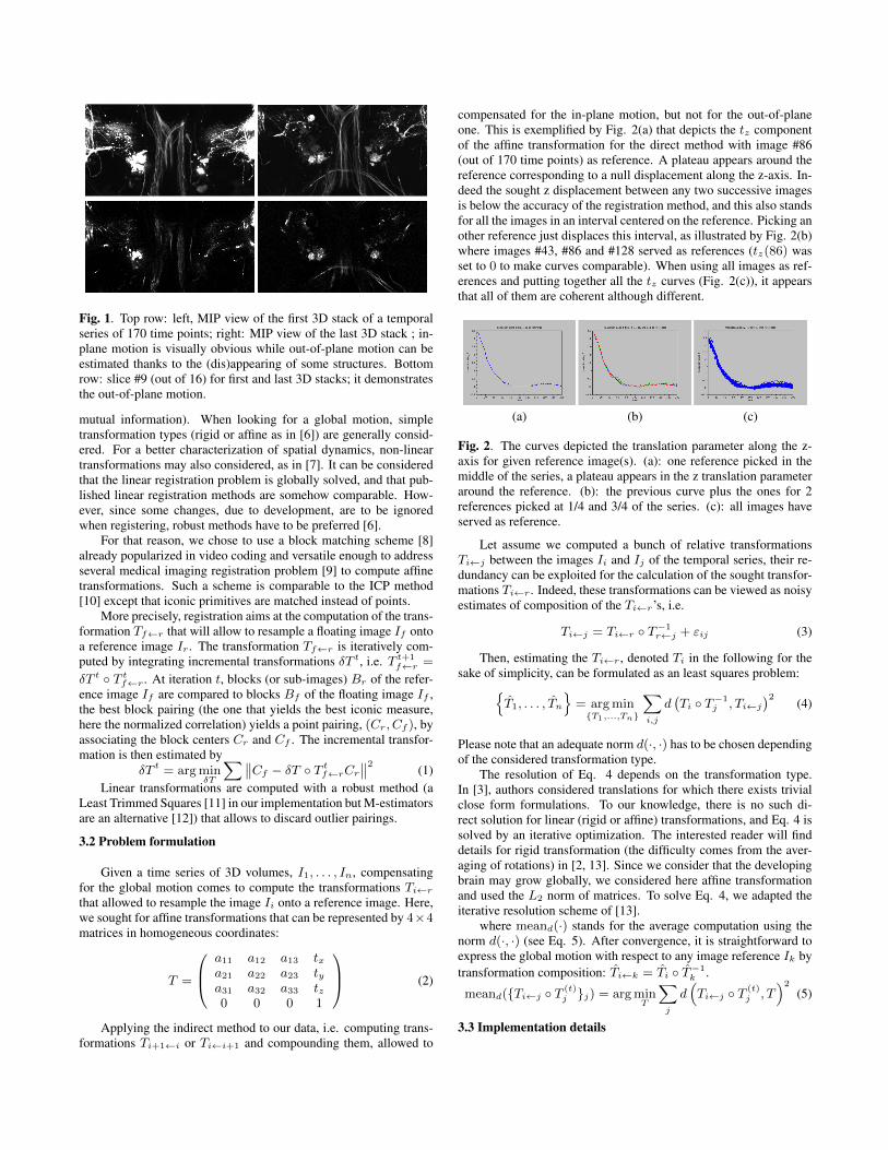
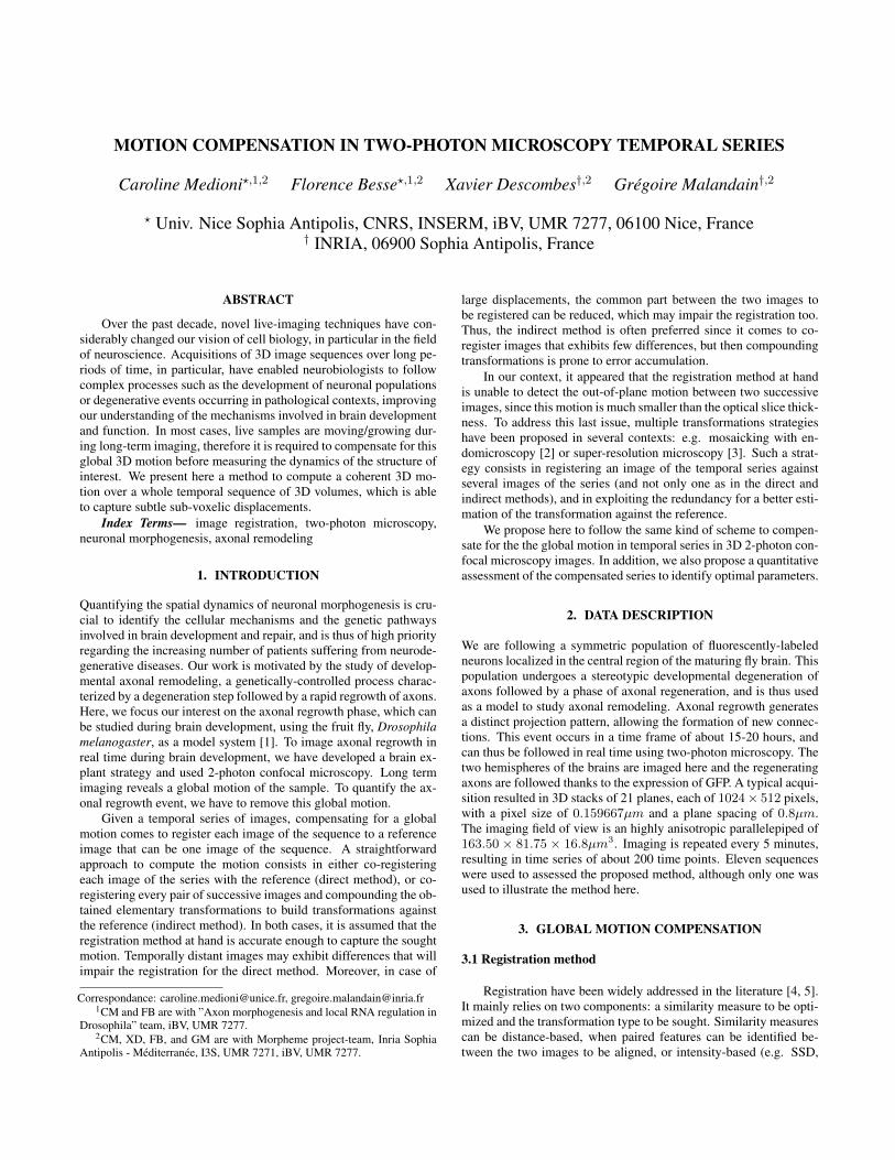
Fig. 1. Top row: left, MIP view of the first 3D stack of a temporalseries of 170 time points; right: MIP view of the last 3D stack ; in-plane motion is visually obvious while out-of-plane motion can beestimated thanks to the (dis)appearing of some structures. Bottomrow: slice #9 (out of 16) for first and last 3D stacks; it demonstratesthe out-of-plane motion.

mutual information). When looking for a global motion, simpletransformation types (rigid or affine as in [6]) are generally consid-ered. For a better characterization of spatial dynamics, non-lineartransformations may also considered, as in [7]. It can be consideredthat the linear registration problem is globally solved, and that pub-lished linear registration methods are somehow comparable. How-ever, since some changes, due to development, are to be ignoredwhen registering, robust methods have to be preferred [6].

For that reason, we chose to use a block matching scheme [8]already popularized in video coding and versatile enough to addressseveral medical imaging registration problem [9] to compute affinetransformations. Such a scheme is comparable to the ICP method[10] except that iconic primitives are matched instead of points.

More precisely, registration aims at the computation of the trans-formation Tf←r that will allow to resample a floating image If ontoa reference image Ir . The transformation Tf←r is iteratively com-puted by integrating incremental transformations δT t, i.e. T t+1

f←r =

δT t T tf←r . At iteration t, blocks (or sub-images) Br of the refer-ence image If are compared to blocks Bf of the floating image If ,the best block pairing (the one that yields the best iconic measure,here the normalized correlation) yields a point pairing, (Cr, Cf ), byassociating the block centers Cr and Cf . The incremental transfor-mation is then estimated by

δT t = arg minδT

∑∥∥Cf − δT T tf←rCr∥∥2 (1)Linear transformations are computed with a robust method (a

Least Trimmed Squares [11] in our implementation but M-estimatorsare an alternative [12]) that allows to discard outlier pairings.

3.2 Problem formulation

Given a time series of 3D volumes, I1, . . . , In, compensatingfor the global motion comes to compute the transformations Ti←rthat allowed to resample the image Ii onto a reference image. Here,we sought for affine transformations that can be represented by 4×4matrices in homogeneous coordinates:

T =

a11 a12 a13 txa21 a22 a23 tya31 a32 a33 tz0 0 0 1

(2)

Applying the indirect method to our data, i.e. computing trans-formations Ti+1←i or Ti←i+1 and compounding them, allowed to

compensated for the in-plane motion, but not for the out-of-planeone. This is exemplified by Fig. 2(a) that depicts the tz componentof the affine transformation for the direct method with image #86(out of 170 time points) as reference. A plateau appears around thereference corresponding to a null displacement along the z-axis. In-deed the sought z displacement between any two successive imagesis below the accuracy of the registration method, and this also standsfor all the images in an interval centered on the reference. Picking another reference just displaces this interval, as illustrated by Fig. 2(b)where images #43, #86 and #128 served as references (tz(86) wasset to 0 to make curves comparable). When using all images as ref-erences and putting together all the tz curves (Fig. 2(c)), it appearsthat all of them are coherent although different.

(a) (b) (c)

Fig. 2. The curves depicted the translation parameter along the z-axis for given reference image(s). (a): one reference picked in themiddle of the series, a plateau appears in the z translation parameteraround the reference. (b): the previous curve plus the ones for 2references picked at 1/4 and 3/4 of the series. (c): all images haveserved as reference.

Let assume we computed a bunch of relative transformationsTi←j between the images Ii and Ij of the temporal series, their re-dundancy can be exploited for the calculation of the sought transfor-mations Ti←r . Indeed, these transformations can be viewed as noisyestimates of composition of the Ti←r’s, i.e.

Ti←j = Ti←r T−1r←j + εij (3)

Then, estimating the Ti←r , denoted Ti in the following for thesake of simplicity, can be formulated as an least squares problem:

T1, . . . , Tn

= arg minT1,...,Tn

∑i,j

d(Ti T−1

j , Ti←j)2

(4)

Please note that an adequate norm d(·, ·) has to be chosen dependingof the considered transformation type.

The resolution of Eq. 4 depends on the transformation type.In [3], authors considered translations for which there exists trivialclose form formulations. To our knowledge, there is no such di-rect solution for linear (rigid or affine) transformations, and Eq. 4 issolved by an iterative optimization. The interested reader will finddetails for rigid transformation (the difficulty comes from the aver-aging of rotations) in [2, 13]. Since we consider that the developingbrain may grow globally, we considered here affine transformationand used the L2 norm of matrices. To solve Eq. 4, we adapted theiterative resolution scheme of [13].

where meand(·) stands for the average computation using thenorm d(·, ·) (see Eq. 5). After convergence, it is straightforward toexpress the global motion with respect to any image reference Ik bytransformation composition: Ti←k = Ti T−1

k .

meand(Ti←j T (t)j j) = arg min

T

∑j

d(Ti←j T (t)

j , T)2

(5)

3.3 Implementation details

Given initial transformations T (0)1 , . . . , T

(0)n ;

repeatfor i = 1 . . . n do

T(t+1)i = meand

(Ti←j T (t)

j j)

endRegularization of the T (t+1)

i until maximum number of iterations tmax is reached;

For a practical implementation of the above iterative optimiza-tion, several choices have to be made.1. The initial guess of the transformations T (0)

1 , . . . , T(0)n . Since

only small displacements are expected, these transformations are setto the identity transformation. Otherwise, transformations with re-spect to a reference (direct method) can be chosen too.2. The choice of the pairwise transformations Ti←j . The more thetransformations, the more costly the computations. We pick one im-age out of 5, i.e. j ∈ 1, 6, . . . to serve as references and reg-ister the neighboring images Ii with i ∈ [j − N, j + N ] ∪ [1, n]for various values of N . When N is equal to the temporal serieslength n, these intervals span the whole series, meaning that all pair-wise the n − 1 registrations against Ij are done. We investigatedN ∈ 10, 30, 50, 70, 100, n.3. The computation of the average meand(Ti←j T (t)

j j). It isnothing but a least squares estimation. Since some registrations mayexhibit a large error (particularly if the common support of images tobe registered is small), robust estimation (i.e. least trimmed squares)may be preferred.4. The number of iterations tmax. Although the iterative optimiza-tion of Eq. 4 is quite fast (because we are dealing with linear trans-formations; this may not be the case with non-linear ones), perform-ing too many iterations is not critical. However, we have to makesure that enough iterations are done to reach convergence.5. Regularization of the T (t+1)

i . A continuous smooth globalmotion is expected. To ensure or enforce the smooth variation of thesought transformations with respect to time, we investigate whetheran explicit smoothing step is required or not. We tested a Gaussianregularization with a standard deviation of 10 minutes (the time stepbetween 2 acquisitions is of 5 minutes).

3.1. Result quantitative assessment

To compare different parameter settings, it is mandatory to as-sess/compare quantitatively the results obtained after global motioncompensation. If the global motion compensation performs well, theintensity of a point M after compensation should not change duringthe acquisition duration (axon growth phenomenons are neglectedbecause of their sparsity, and it is assumed that intensity changesdue to bleaching are less important that intensity variations due tomaterial displacement), thus that Ii Ti(M) ' Ij Tj(M)∀i, j,Mstands, where Ii Ti denotes the image Ii resampled by Ti into thereference frame. The standard deviation of values taken by M (aftercompensation) over the resampled images Ii Ti seemed then tobe a relevant objective measure of motion compensation for the pointM . To assess globally the motion compensation, we computed theprobability density function of the standard deviation values. Thebetter the motion compensation, the smaller the standard deviationvalues. Because of motion, all physical point M imaged in the firstimage I1 may not be imaged during the whole acquisition. We re-stricted the standard deviation computation to the points belongingto the common acquisition space Ω. Let S be the acquisition space

of the 3-D stacks Ii, S = [1 . . . X] × [1 . . . Y ] × [1 . . . Z], and 1Iby the indicator image of the stacks, i.e.

1I(M) =

1 if M ∈ S0 else (6)

We have Ω =⋂i 1I Ti. We computed the probability density

function (pdf) of the standard deviation of the points M ∈ Ω overthe whole resampled sequence Ii Tii (see Fig. 3, left). A centile(say 0.8) of the probability density function is used as the objec-tive quality measure. The cumulative probability density function,cpdf(·) (see Fig. 3, right) exemplifies graphically how to assessthe motion compensation: the leftmost curve indicates the smallerstandard deviation, and σp such that cpdf(σp) = 0.8 is the qualitymeasure for a given parameter settings.

Fig. 3. Left: standard deviation probability density function over thewhole resampled sequence Ii Ti for several parameter settings(the dashed curve corresponds to original data). Right: cumulativestandard deviation probability density function.

4. RESULTS

Fig. 4. Quality measures σp for different parameter settings.

Fig. 4 summarizes the quality measures for different parametersettings for one data set. This is also representative for the 20 datasets we have at hand. From our observations, we can derive somegeneral trends:• There is a floor value for the quality measure: visual inspection ofthe resampled temporal series reconstructed for this floor value didnot reveal any noticeable differences.• The more the iterations, the faster the convergence towards thefloor value.• The more the transformations Ti←j (the larger the N ), the fasterthe convergence towards the floor value.• Before the floor value is reached, a robust estimation of the trans-formation average seems to perform slightly better than non-robustestimation, and transformation regularization seems to slightly dete-riorate the quality measure.

From these observations, we choose to perform 20 iterations, touse all pairwise transformations Ti←j (N = n), without robust esti-mation of the average nor regularization of the transformation. Theevolution of the parameters of the estimated global motion (affinetransformations) Ti with respect to time are depicted in Fig. 5 wherethey can be compared to pairwise transformations Ti←j . Unsurpris-ingly, it appears that the parameters involving the third dimension,i.e. the z-axis, are the ones (see e.g. a33, 3rd column and 3rd row)for which there is the more dispersion in the Ti←j .

We choose the first image as reference, and the Ti’s allow toresample the images Ii’s onto I1. Fig. 6 presents the resampled lastimage, I170 T170, which is to be compared to the first one I1. Itdemonstrates visually the global 3D motion compensation.

Fig. 5. Purple curves depicted the evolution of pairwise transforma-tion parameters (one curve pear each element of the 3 upper rows ofmatrix T , see Eq. 2; the last row corresponds then to the translationcomponent) for all references, while blue curves depicted the motionestimation.

Fig. 6. Top row: left, MIP view of the first 3D stack of a temporalseries of 170 time points; right: MIP view of the last resampled 3Dstack ; in-plane motion correction can be visually estimated. Bottomrow: slice #9 (out of 16) for first and last resampled 3D stacks; theout-of-plane motion has been quite well compensated since similarstructures appear in both slices.

5. CONCLUSION

We propose a method for global motion compensation that is basedon multiple transformations averaging. The proposed results demon-strated its ability to correct for sub-voxelic displacement in temporal

series. Moreover, its versatile design makes it able to handle a vari-ety of transformation classes. In addition, we also propose a qualitymeasure for compensated series. This allowed us to objectively com-pare different parameter settings and identify a default setting fordata processing. Thanks to the drift correction, we are now able toquantitatively measure the axonal regrowth without being perturbedby the global motion of the sample. This opens new perspectives tounderstand how axons are able to regenerate both in normal devel-opmental and in pathological context.Acknowledgments: this work was supported by the French Govern-ment (National Research Agency, ANR) through the ”Investmentsfor the Future” LABEX SIGNALIFE: program reference # ANR-11-LABX-0028-01

6. REFERENCES

[1] S. Lenz, P. Karsten, J.B. Schulz, and A. Voigt, “Drosophila asa screening tool to study human neurodegenerative diseases,”J Neurochem, vol. 127, no. 4, pp. 453–60, November 2013.

[2] T. Vercauteren, A. Perchant, G. Malandain, X. Pennec, andN. Ayache, “Robust mosaicing with correction of motion dis-tortions and tissue deformation for in vivo fibered microscopy,”Medical Image Analysis, vol. 10, no. 5, pp. 673–692, 2006.

[3] Y. Wang, J. Schnitzbauer, Z. Hu, X. Li, Y. Cheng, Z.L.Huang, and B. Huang, “Localization events-based sample driftcorrection for localization microscopy with redundant cross-correlation algorithm,” Opt Express, vol. 22, no. 13, pp.15982–91, June 2014.

[4] J.B. Maintz and M.A. Viergever, “A survey of medical imageregistration,” Med Image Anal, vol. 2, no. 1, pp. 1–36, 1998.

[5] B. Zitova and J. Flusser, “Image registration methods: a sur-vey,” Image Vis Comput, vol. 21, no. 11, pp. 977–1000, 2003.

[6] S. Ozere, P. Bouthemy, F. Spindler, P. Paul-Gilloteaux, andC. Kervrann, “Robust parametric stabilization of movingcells with intensity correction on light microscopy image se-quences,” in ISBI, 2013, pp. 464–467.

[7] D. Sorokin, M. Tektonidis, K. Rohr, and P. Matula, “Non-rigidcontour-based temporal registration of 2d cell nuclei imagesusing the navier equation,” in ISBI, 2014, pp. 746–749.

[8] J.R. Jain and A.K. Jain, “Displacement measurement and itsapplication in interframe image coding,” IEEE Trans. Com-mun., vol. 29, pp. 17991808, 1981.

[9] S. Ourselin, A. Roche, S. Prima, and N. Ayache, “Block match-ing: A general framework to improve robustness of rigid reg-istration of medical images,” in MICCAI. 2000, vol. 1935 ofLNCS, pp. 557–566, Springer.

[10] P.J. Besl and N.D. McKay, “A method for registration of 3-Dshapes,” IEEE Transactions on Pattern Analysis and MachineIntelligence, vol. 14, no. 2, pp. 239–256, February 1992.

[11] P.J. Rousseeuw and A.M. Leroy, Robust Regression and Out-lier Detection, John Wiley & Sons, New-York, 1987.

[12] J.M. Odobez and P. Bouthemy, “Robust multiresolution esti-mation of parametric motion models,” J Vis Commun ImageRepresent, vol. 6, no. 4, pp. 348–365, 1995.

[13] R. Hartley, J. Trumpf, Y. Dai, and H. Li, “Rotation averaging,”Int J Comput Vis, vol. 103, no. 3, pp. 267–305, 2013.