Seediscussions,stats,andauthorprofilesforthispublicationat:https://www.researchgate.net/publication/282181999

Motility-DrivenGlassandJammingTransitionsinBiologicalTissues

ArticleinPhysicalReviewX·September2015

ImpactFactor:9.04·DOI:10.1103/PhysRevX.6.021011·Source:arXiv

CITATION

1

READS

61

4authors:

DapengBi

TheRockefellerUniversity

23PUBLICATIONS220CITATIONS

SEEPROFILE

XingboYang

NorthwesternUniversity

6PUBLICATIONS43CITATIONS

SEEPROFILE

MCristinaMarchetti

SyracuseUniversity

174PUBLICATIONS3,666CITATIONS

SEEPROFILE

M.LisaManning

SyracuseUniversity

39PUBLICATIONS638CITATIONS

SEEPROFILE

Allin-textreferencesunderlinedinbluearelinkedtopublicationsonResearchGate,

lettingyouaccessandreadthemimmediately.

Availablefrom:DapengBi

Retrievedon:22May2016

Motility-driven glass and jamming transitions in biological tissues

Dapeng Bi1,2, Xingbo Yang1,2, M. Cristina Marchetti1,4, M. Lisa Manning1,4

1Department of Physics, Syracuse University, Syracuse, NY, USA2Present address: Center for Studies in Physics and Biology, Rockefeller University, NY ,USA

3Present address: McCormick School of Engineering, Northwestern University, Evanston, IL4Syracuse Biomaterials Institute, Syracuse, NY, USA

Cell motion inside dense tissues governs many biological processes, including embryonic development andcancer metastasis, and recent experiments suggest that these tissues exhibit collective glassy behavior. To makequantitative predictions about glass transitions in tissues, we study a self-propelled Voronoi (SPV) model thatsimultaneously captures polarized cell motility and multi-body cell-cell interactions in a confluent tissue, wherethere are no gaps between cells. We demonstrate that the model exhibits a jamming transition from a solid-likestate to a fluid-like state that is controlled by three parameters: the single-cell motile speed, the persistencetime of single-cell tracks, and a target shape index that characterizes the competition between cell-cell adhesionand cortical tension. In contrast to traditional particulate glasses, we are able to identify an experimentallyaccessible structural order parameter that specifies the entire jamming surface as a function of model parameters.We demonstrate that a continuum Soft Glassy Rheology model precisely captures this transition in the limit ofsmall persistence times, and explain how it fails in the limit of large persistence times. These results providea framework for understanding the collective solid-to-liquid transitions that have been observed in embryonicdevelopment and cancer progression, which may be associated with Epithelial-to-Mesenchymal transition inthese tissues.

Recent experiments have revealed that cells in dense bio-logical tissues exhibit many of the signatures of glassy ma-terials, including caging, dynamical heterogeneities and vis-coelastic behavior [1–5]. These dense tissues, where cells aretouching one another with minimal spaces in between, arefound in diverse biological processes including wound heal-ing, embryonic development, and cancer metastasis.

In many of these processes, tissues undergo an Epithelial-to-Mesenchymal Transition (EMT), where cells in a solid-like, well-ordered epithelial layer transition to a mesenchy-mal, migratory phenotype with less well-ordered cell-cell in-teractions [6, 7], or an inverse process, the Mesenchymal-to-Epithelial Transition (MET). Over many decades, detailed cellbiology research has uncovered many of the signaling path-ways involved in these transitions [8, 9], which are importantin developing treatments for cancer and congenital disease.

Most previous work on EMT/MET has focused, however,on properties and expression levels in single cells or pairs ofcells, leaving open the interesting question of whether there isa collective aspect to these transitions: Are some features ofEMT/MET generated by large numbers of interacting cells?Although there is no definitive answer to this question, severalrecent works have suggested that EMT might coincide with acollective solid-to-liquid jamming transition in biological tis-sues [5, 10–12]. Therefore, our goal is to develop a frameworkfor jamming and glass transitions in a minimal model that ac-counts for both cell shapes and cell motility, in order to makepredictions that can quantitatively test this conjecture.

Jamming occurs in non-biological particulate systems (suchas granular materials, polymers, colloidal suspensions, andfoams) when their packing density is increased above somecritical threshold, and glass transitions occur when the fluid iscooled below a critical temperature. Over the past 20 yearsthese phenomena have been unified by “jamming phase dia-grams” [13, 14].

Building on these successes, researchers have recently used

self-propelled particle (SPP) models to describe dense bio-logical tissues [15–17]. These models are similar to thosefor inert particulate matter – cells are represented as disks orspheres that interact with an isotropic soft repulsive potential –but unlike Brownian particles in a thermal bath, self-propelledparticles exhibit persistent random walks. Just like in thermalsystems, SPP models exhibit a jamming transition at a criticalpacking density φG, but this critical density is slightly alteredby the persistence time of the random walks [17–21].

During many biological processes, however, a tissue re-mains at confluence (packing fraction equal to unity) whileit changes from a liquid-like to a solid-like state or vice-versa.For example, in would-healing, cells collectively organize toform a ‘moving sheet’ without any change in their packingdensity [22], and during vertebrate embryogenesis mesendo-derm tissues are more fluid-like than ectoderm tissues, despiteboth having packing fraction equal to unity [1].

Recently, Bi and coworkers [23] have demonstrated that thewell-studied vertex model for 2-D confluent tissues [24–29]exhibits a rigidity transition in the limit of zero cell motil-ity. Specifically, the rigidity of the tissue vanishes at a crit-ical balance between cortical tension and cell-cell adhesion.An important insight is that this transition depends sensitivelyon cell shapes, which are well-defined in the vertex model.While promising, vertex models are difficult to compare tosome aspects of experiments because they do not incorporatecell motility.

In this work, we bridge the gap between the confluent tis-sue mechanics and cell motility by studying a hybrid betweenthe vertex model and the SPP model, that we name Self-Propelled-Voronoi (SPV) model. A similar model was in-troduced by Li and Sun [30], and cellular Potts models alsobridge this gap [31, 32], although glass transitions have notbeen carefully studied in any of these hybrid systems.

2

��-�

��-�

��-�

���

���

��� ��� ��� ��� �������

����

����

����

����

����

h�r2

(t)i

Fs(q

,t)

t

��-�

��-�

��-�

���

���

p0

De↵

��-�

��-�

��-�

���

���

��-�

��-�

��-�

���

���

��-�

��-�

��-�

���

���

A

B

C

D

decreasing p0

decreasing p0

■ ■ ■ ■ ■ ■ ■

■

■

■■ ■

��� ��� ��� ��� ��� �������

����

����

FIG. 1. Analysis of glassy behavior. (A) The mean-squared displacement of cell centers for Dr = 1 and v0 = 0.1 and various values of p0(top to bottom: p0 = 3.85,3.8,3.75,3.7,3.65,3.5) show the onset of dynamical arrest as p0 is decreased indicating a glass transition. Thedashed lines indicate a slope of 2(ballistic) and 1(diffusive) on log-log plot. (B) The self-intermediate scattering function at the same values ofp0 show in (A) shows the emergence of caging behavior at the glass transition. (C) The effective self-diffusivity as function of p0 at v0 = 0.1.At the glass transition De f f becomes nonzero. (D)The cell displacement map in SPV model for p0 = 3.75, v0 = 0.1 and Dr = 1 over a timewindow t ≈ 103 corresponding to the structural relaxation at which Fs(q, t) = 1/2.

I. THE SPV MODEL

While the vertex model describes a confluent tissue as apolygonal tiling of space where the degrees of freedom arethe vertices of the polygons, the SPV model identifies eachcell only using the center (rrri) of Voronoi cells in a Voronoitessellation of space [33]. For a tissue containing N-cells, theinter-cellular interactions are captured by a total energy whichis the same as that in the vertex model. Since the tessellation iscompletely determined by the {rrri}, the total tissue mechanicalenergy can be fully expressed as E = E({rrri}):

E =N

∑i=1

[KA(A(ri)−A0)

2 +KP(P(ri)−P0)2] . (1)

The term quadratic in cell area A(ri) results from a combi-nation of cell volume incompressibility and the monolayer’sresistance to height fluctuations [26]. The term involvingthe cell perimeter P(ri) originates from active contractilityof the acto-myosin sub-cellular cortex (quadratic in perime-ter) and effective cell membrane tension due to cell-cell ad-hesion and cortical tension (both linear in perimeter). Thisgives rise to an effective target shape index that is dimension-less: p0 = P0/

√A0. KA and KP are the area and perimeter

moduli, respectively. For the remainder of this manuscript weassume p0 is homogenous across a tissue, although heteroge-neous properties are also interesting to consider [34].

In the vertex model [23], a rigidity transition takes place at acritical value of p0 = p∗0 ≈ 3.81, below which the cortical ten-

sion dominates over cell-cell adhesion and the tissue behaveslike a elastic solid; above p∗0, cell-cell adhesion dominates andthe tissue rigidity vanishes. While the energy functional forcell-cell interactions is identical in the vertex and SPV models,the two are truly distinct: the local minimum energy states ofthe vertex model are not guaranteed to be similar to a Voronoitessellation of cell centers, although we do find them to bevery similar in practice. Therefore, we are also interested inwhether a rigidity transition in the SPV model coincides withthe rigidity transition of the vertex model.

We define the effective mechanical interaction force expe-rienced by cell i as FFF i = −∇∇∇iE (see Appendix A for details).In contrast to particle-based models, FFF i is non-local and non-additive: FFF i cannot be expressed as a sum of pairwise forcebetween cells i and its neighboring cells.

In addition to FFF i, cells can also move due to self-propelledmotility. Just as in SPP models, we assign a polarity vectornnni = (cosθi,sinθi) to each cell; along nnni the cell exerts a self-propulsion force with constant magnitude v0/µ, where µ isthe mobility (the inverse of a frictional drag). Together theseforces control the over-damped equation of motion of the cellcenters rrri

drrri

dt= µFFF i + v0nnni. (2)

The polarity is a minimal representation of the front/rearcharacterization of a motile cell [31]. While the precise mech-anism for polarization in cell motility is an area of intense

3

A B

■ ■ ■ ■ ■ ■ ■ ■ ■ ■ ■ ■ ■ ■ ■ ■ ■■ ■ ■ ■ ■ ■ ■ ■ ■ ■ ■ ■ ■ ■ ■ ■ ■■ ■ ■ ■ ■ ■ ■ ■ ■ ■ ■ ■ ■ ■ ■ ■ ■■ ■ ■ ■ ■ ■ ■ ■ ■ ■ ■ ■ ■ ■ ■ ■■ ■ ■ ■ ■ ■ ■ ■ ■ ■ ■ ■ ■ ■ ■■ ■ ■ ■ ■ ■ ■ ■ ■ ■ ■ ■ ■ ■■ ■ ■ ■ ■ ■ ■ ■ ■ ■ ■ ■ ■ ■■ ■ ■ ■ ■ ■ ■ ■ ■ ■ ■ ■ ■■ ■ ■ ■ ■ ■ ■ ■ ■ ■ ■■ ■ ■ ■ ■ ■ ■ ■ ■ ■ ■■ ■ ■ ■ ■ ■ ■ ■ ■■ ■ ■ ■ ■ ■ ■ ■■ ■ ■ ■ ■ ■■ ■ ■ ■■ ■

● ● ● ●● ● ● ●● ● ● ●

● ● ● ● ●● ● ● ● ● ●

● ● ● ● ● ● ●● ● ● ● ● ● ●

● ● ● ● ● ● ● ●● ● ● ● ● ● ● ● ● ●● ● ● ● ● ● ● ● ● ●

● ● ● ● ● ● ● ● ● ● ● ●● ● ● ● ● ● ● ● ● ● ● ● ●

● ● ● ● ● ● ● ● ● ● ● ● ● ● ●● ● ● ● ● ● ● ● ● ● ● ● ● ● ● ● ●

● ● ● ● ● ● ● ● ● ● ● ● ● ● ● ● ● ● ●● ● ● ● ● ● ● ● ● ● ● ● ● ● ● ● ● ● ● ● ●● ● ● ● ● ● ● ● ● ● ● ● ● ● ● ● ● ● ● ● ●

��� ��� ��� ��� ��� ������

���

���

���

��

� �

Solid

Fluid

FIG. 2. (A) Glassy phase diagram for confluent tissues as function of cell motility v0 and target shape index p0 at fixed Dr = 1. Blue datapoints correspond to solid-like tissue with vanishing De f f ; orange points correspond to flowing tissues (finite De f f ). The dynamical glasstransition boundary also coincides with the locations in phase space where the structural order parameter q = 〈p/√a〉= 3.81 (red line). In thesolid phase, q≈ 3.81 and q > 3.81 in the fluid phase. (B) Instantaneous tissue snapshots show the difference in cell shape across the transition.Cell tracks also show dynamical arrest due to caging in the solid phase and diffusion in the fluid phase.

study, here we model its dynamics as a unit vector that under-goes random rotational diffusion

∂tθi = ηi(t)

〈ηi(t)η j(t ′)〉= 2Drδ(t− t ′)δi j(3)

where θi is the polarity angle that defines nnni, and ηi(t) is awhite noise process with zero mean and variance 2Dr. Thevalue of angular noise Dr determines the memory of stochasticnoise in the system, giving rise to a persistence time scale τ =1/Dr for the polarization vector n. For small Dr � 1, thedynamics of n is more persistent than the dynamics of thecell position. At large values of Dr, i.e. when 1/Dr becomesthe shortest timescale in the model, Eq. (2) approaches simpleBrownian motion.

The model can be non-dimensionalized by expressing alllengths in units of

√A0 and time in units of 1/(µKAA0). There

are three remaining independent model parameters: the selfpropulsion speed v0, the cell shape index p0, and the rota-tional noise strength Dr. We simulate a confluent tissue un-der periodic boundary conditions with constant number ofN = 400 cells (no cell divisions or apoptosis) and assume thatthe average cell area coincides with the preferred cell area,i.e. 〈Ai〉 = A0. This approximates a large confluent tissue inthe absence of strong confinement. We numerically simulatethe model using molecular dynamics by performing 105 inte-gration steps at step size ∆t = 10−1 using Euler’s method. Adetailed description of the SPV implementation can be foundin the Appendix Sec. A.

II. CHARACTERIZING GLASSY BEHAVIOR

We first characterize the dynamics of cell motion within thetissue by analyzing the mean-squared displacement (MSD) ofcell trajectories. In Fig. 1(a), we plot the MSD as functionof time, for tissues at various values of p0 and fixed v0 = 0.1and Dr = 1. The MSD exhibits ballistic motion (slope =2on a log-log plot) at short times, and plateaus at intermedi-ate timescales. The plateau is an indication that cells are be-coming caged by their neighbors. For large values of p0, theMSD eventually becomes diffusive (slope =1), but as p0 isdecreased, the plateau persists for increasingly longer times.This indicates dynamical arrest due to caging effects and bro-ken ergodicity, which is a characteristic signature of glassydynamics.

Another standard method for quantifying glassy dynamicsis the self-intermediate scattering function [35]: Fs(q, t) =⟨

ei~q·∆~r(t)⟩. Glassy systems possess a broad range of relax-

ation timescales, which show up as a long plateau in Fs(t)when it is analyzed at a lengthscale q comparable to the near-est neighbor distance. Fig 1 (b) illustrates precisely this be-havior in the SPV model, when |~q| = 2π/r0, where r0 is theposition of the first peak in the pair correlation function. Theaverage 〈...〉 is taken temporally as well as over angles of ~q.Fs(t) also clearly indicates that there is a glass transition as afunction of p0: at high p0 values Fs approaches zero at longtimes, indicating that the structure is changing and the tissuebehaves as a viscoelastic liquid. At lower values of p0, Fs re-mains large at all timescales, indicating that the structure is ar-rested and the tissue is a glassy solid. Fig 1 (d) demonstrates

4

that at the structural relaxation time, the cell displacementsshow collective behavior across large lengthscales suggestingstrong dynamical heterogeneity. This is strongly reminiscentof the ‘swirl’ like collective motion seen in experiment in ep-ithelial monolayers [3, 4].

A. A dynamical order parameter for the glass transition

Although the phase space for this model is three dimen-sional, we now study the model at a fixed value of Dr = 1.

We then search for a dynamical order parameter that dis-tinguishes between the glassy and fluid states as a func-tion of the two remaining model parameters,(v0, p0). Acandidate order parameter is the self-diffusivity Ds: Ds =

limt→∞〈∆r(t)2〉/(4t). For practicality, we calculate Ds usingsimulation runs of 105 time steps, chosen to be much longerthan the typical caging timescale in the fluid regime. Wepresent the self-diffusivity in units of D0 = v2

0/(2Dr), which isthe free diffusion constant of an isolated cell. De f f = Ds/D0then serves as an accurate dynamical order parameter that dis-tinguishes a fluid state from a sold(glassy) state in the spaceof (v0, p0), matching the regimes identified using the MSDand Fq. In Fig. 2, the fluid region is characterized by a finitevalue of De f f and De f f drops below a noise floor of ∼ 10−3

as the glass transition is approached. In practice, we labelmaterials with De f f > 10−3 as fluids indicated by a yellowdot, and those with De f f ≤ 10−3 as solids indicated by bluesquares. Importantly, we find that the SPV model in the limitof zero cell motility shares a rigidity transition with the vertexmodel [23] at p0 ≈ 3.81, and that this rigidity transition con-trols a line of glass transitions at finite cell motilities. Typicalcell tracks (Fig. 2) clearly show caging behavior in the glassysolid phase.

B. Cell shape is a structural order parameter for the glasstransition

Previously the shape index q = 〈p/√a〉 was shown to bean excellent order parameter for the confluent tissue rigiditytransition in the vertex model[10]; for p0 < 3.813, q is con-stant ∼ 3.81 and q≈ p0 for p0 > 3.81. Quite surprisingly, wefind that q (which can be easily calculated in experiments orsimulations from a snapshot) can be used as a structural orderparameter for the glass transition for all values of v0, not justat v0 = 0. Specifically, the boundary defined by q = 3.813,shown by the red solid line in Fig. 2 coincides extremely wellwith the glass transition line obtained using the dynamical or-der parameter, shown by the round and square data points.The insets to Fig. 2 also illustrate typical cell shapes: cellsare isotropic on average in the solid phase and anisotropicin the fluid phase. This provides a new explanation of whythe q = 3.813 prediction works perfectly in identifying a jam-ming transition in in-vitro experiments involving primary hu-man tissues, where cells are clearly motile [10]. Although thisprediction was originally developed using a non-motile vertex

model, the results presented here confirm that it should alsowork in tissues with finite cell motility.

III. A THREE-DIMENSIONAL JAMMING PHASEDIAGRAM FOR TISSUES

Having studied the glass transition as function of v0 andp0 at a large value of Dr, we next investigate the full three-dimensional phase diagram by characterizing the effect of Dron tissue mechanics and structure. Dr controls the persistencetime τ = 1/Dr and persistence length or Peclet number Pe ∼v0/Dr of cell trajectories; smaller values of Dr correspond tomore persistent motion.

In Fig. 3(a), we show several 2D slices of the three di-mensional jamming boundary. Solid lines illustrate the phasetransition line identified by the structural order parameterq = 3.813 as function of v0 and p0 for a large range of Dr val-ues (from 10−2 to 103). (In Appendix B 2 we demonstrate thatthe structural transition line q = 3.813 matches the dynamicaltransition line for all studied values of Dr.) In contrast to re-sults for particulate matter [20], this figure illustrates that theglass transition lines meet at a single point (p0 = 3.81) in thelimit of vanishing cell motility, regardless of persistence.

Fig. 3(b) shows an orthogonal set of slices of the jammingdiagram, illustrating how the phase boundary shifts as func-tion of p0 and Dr at various values of v0. This highlights theinteresting result that a solid-like material at high value of Drcan be made to flow simply by lowering its value of Dr.

These slices can be combined to generate a three-dimensional jamming phase diagram for confluent biologicaltissues, shown in Fig. 3(C). This diagram provides a concrete,quantifiable prediction for how macroscopic tissue mechanicsdepends on single-cell properties such as motile force, persis-tence, and the interfacial tension generated by adhesion andcortical tension.

We note that Fig. 3(C) is significantly different from thejamming phase diagram conjectured by Sadati et al [11],which was informed by results from adhesive particulate mat-ter [14]. For example, in particulate matter adhesion enhancessolidification, while in confluent models adhesion increasescell perimeters/surface area and enhances fluidization. In ad-dition, we identify “persistence” as a new axis with a poten-tially significant impact on cell migration rates in dense tis-sues.

To better understand why persistence is so important indense tissues, we first have to characterize the transitions be-tween different cellular structures. In the limit of zero cellmotility, the system can be described by a potential energylandscape where each allowable arrangement of cell neigh-bors corresponds to a metastable minimum in the landscape.There are many possible pathways out of each metastablestate: some of correspond to localized cell rearrangements,while others correspond to large-scale collective modes. Themaximum energy required to transition out of a metastablestate along each pathway is called an energy barrier [29].

We observe that tissue fluidity can increase drastically withincreasing Dr at finite cell speeds. This suggests that different

5

Dr

p0

v0

��� ��� ��� ��� ��� ��� ��� ������

���

���

���

���0.0112520

1000

● ●

●

●

●

●●

● ● ●

■ ■

■

■

■

■■

■ ■ ■

◆ ◆

◆◆

◆

◆ ◆ ◆ ◆ ◆

▲ ▲

▲ ▲

▲▲ ▲ ▲ ▲ ▲

▼ ▼▼ ▼ ▼ ▼ ▼ ▼ ▼ ▼

○○ ○ ○ ○ ○ ○ ○ ○□ □ □ □ □ □ □ □ □ □

��-� ��-� ��� ��� ��� ���

���

���

���

���

���

v0p0

Dr

A B C

p0

v0

1/Dr

Solid-like

FIG. 3. (A) The glass transition in v0− p0 phase space shifts as the persistence time changes. Lines represent the glass transition identifiedby the structural order parameter q = 3.81. The phase boundary collapse to a single point at p∗0 = 3.81, regardless of Dr, in the limit v0→ 0.(B) The glass transition in p0−Dr phase space shifts as a function of v0 (from top to bottom: v0 = 0.02,0.08,0.14,0.2,0.26) (C) The phaseboundary between solid and fluid as function of motility v0, persistence 1/Dr and p0 which is tuned by cell-cell adhesion can be organizedinto a schematic 3D phase diagram in.

Dr = 0.01 10.1

A B C

FIG. 4. (A-C) Instantaneous cell displacements at p0 = 3.65 andv0 = 0.5. They are different from the displacements shown inFig. 1(D) which are averaged over the structural relaxation timescale.(A) At the lowest value of Dr = 0.01, the cells are able to flow bycollectively displacing along the ‘soft’ modes of the system (Ap-pendix. B 1). (B) At Dr = 0.1, collective displacements are lesspronounced. (C) For Dr = 1 and larger, the displacements appeardisordered and uncorrelated.

pathways (with lower energy barriers) must become dynami-cally accessible at higher values of Dr.

One hint about these pathways comes from the instanta-neous cell displacements, shown for different values of Dr inFig. 4. At high values of Dr, (p0 = 3.78, v0 = 0.1) the instan-taneous displacement field is essentially random and largelyuncorrelated, as shown in Fig. 4, and the material is solid-like. There is no collective behavior among cells, and eachcell ‘rattles’ independently near its equilibrium position.

However, as Dr is lowered, the instantaneous displacementfield becomes much more collective (Fig. 4) and the tissuebegins to flow, presumably because these collective displace-ment fields correspond to pathways with lower transition en-ergies.

Two obvious questions remain: How does a lower valueof Dr generate more collective instantaneous displacements?Why should collective instantaneous displacements generi-cally have lower energy barriers? The first question can be

answered by extending ideas first proposed by Henkes, Filyand Marchetti [17] to explain why motion in self-propelledparticle models seems to follow the ‘soft modes’ of a solid.This argument is based on a simple, yet powerful observation:in the limit of zero motility (v0 = 0), a solid-like state will havea well-defined set of normal modes of vibration (with frequen-cies {ων}), and a corresponding set of eigenvectors ({eν}) thatforms a complete basis. At higher motilities (v0 > 0) near theglass transition, the motion of particles in the system can beexpanded in terms of the eigenvectors. As discussed in Ap-pendix B 1, one can use this observation to show that in thelimit of Dr → 0, motion along the lowest frequency eigen-modes is amplified – the amplitude along each mode is pro-portional to 1/ω2

ν). These low-frequency normal modes areprecisely the collective displacements observed for low Dr.

The second question is more difficult to answer because itis impossible to enumerate all of the possible transition path-ways and energy barriers in a disordered material. However,a partial answer comes from recent work in disordered par-ticulate matter showing that low-frequency normal modes dohave significantly lower energy barriers [36, 37] than higherfrequency normal modes. This is an interesting avenue forfuture research.

IV. A CONTINUUM MODEL FOR GLASS TRANSITIONSIN TISSUES

Although continuum hydrodynamic equations of motionhave been developed by coarse graining SPP models in thedilute limit, there is no existing continuum model for a denseactive matter system near a glass transition. Here we proposethat a simple trap [38] or Soft Glassy Rheology (SGR) [39]model provides an excellent continuum approximation for thephase behavior in the large Dr Brownian regime, but fails inthe small Dr limit.

For large Dr it is known that partilce behave like Brownian

6

particles with an effective temperature Te f f = v20/2µDr [18].

This mapping becomes exact when Dr→∞ at fixed “effectiveinertia” (µDr)

−1 [21]. In other words, like in granular sys-tems [40, 41], the effective temperature in SPP is dominatedby kinetic effects. Guided by this result we conjecture thatin our model the temperature also scale quadratically with thevelocity,

Te f f ∝ cv20. (4)

Physically, this effective temperature gives the amount of en-ergy available for individual cells to vibrate within their cageor ‘trap’.

The next important question is how to characterize the ‘trapdepths’, or energy barriers between metastable states. In theBrownian regime (large Dr) there is no dynamical mechanismfor the cells to organize collectively, and therefore a reason-able assumption is that the rearrangements are small and lo-calized.

■■■■■■■■■■■■■■■■■■■■■■

■■■■■■■■■■■■■■■■■■■■■

■■■■■■■■■■■■■■■■■■■■

■■■■■■■■■■■■■■■■■■■

■■■■■■■■■■■■■■■■■

■■■■■■■■■■■■■■■■

■■■■■■■■■■■■■■

■■■■■■■■■■■

■■■■■■��� ��� ��� ��� ��� ����

�

�

�

�

p0

■

■

■ ■ ■ ■ ■��� ��� ��� ����

�

�

�

�

��

DrTef

f

L2

FIG. 5. Comparison between SPV glass transition and an analyticprediction based on a Soft Glass Rheology (SGR) continuum model.The dashed line corresponds to an SGR prediction with no fit param-eter based on previously measured vertex model trap depths [29].Data points correspond to SPV simulations with Dr = 10−3 andwhere we have defined Te f f = cv2

0 with c= 0.1 as the best-fit normal-ization parameter. Blue points correspond to simulations which aresolid-like, with De f f < 10−3, and the boundary of these points definethe observed SPV glass transition line. (Inset) L2 difference betweenSPV glass transition line (at best-fit value of c) and the predicted SGRtransition line at various values of Dr. The SGR prediction based onlocalized T1 trap depths works well in the high Dr limit, but not inthe low Dr limit.

In [29], some of us explicitly calculated the statistics of en-ergy barriers for localized rearrangements in the equilibriumvertex model. In the 2D vertex model, one can show thatlocalized rearrangements must occur via so-called T1 tran-sitions [42]. Using a trap model [38] or Soft Glassy Rheol-ogy(SGR) [39] framework, we were able to use these statis-tics to generate an analytic prediction, with no fit parameters,for the glass transition temperature Tg as function of p0.

To see if the SGR prediction for the glass transition holdsfor the SPV model in the large Dr limit, we simply overlay

the data points corresponding to glassy states from the SPVmodel with the glass transition Tg line predicted in [29]. Thereis one fitting parameter c that characterizes the proportionalityconstant in Eq. 4. Fig 5, shows that the SPV data for Dr = 103

is in excellent agreement with our previous SGR prediction.The reason the effective temperature SGR model works

here is that, like in SPP models of spherical active Browniancolloids, the angular dynamics of each cell evolves indepen-dently of cell-cell interactions and of the angular dynamics ofother cells. An additional alignment interaction that couplesthe angular and translational dynamics may therefore modifythis behavior.

To our knowledge, this is the first time that a SGR/trapmodel prediction has been precisely tested in any glassy sys-tem. This is because, unlike most glass models, we can enu-merate all of the trap depths for localized transition paths inthe vertex model.

However, for small values of Dr, we have shown that celldisplacements are dominated by collective normal modes, andtherefore the energy barriers for localized T1 transitions areprobably irrelevant in this regime. The inset to Fig 5 showsthe deviation (L2-norm) between glass transition lines in theSPV model and T1-based SGR prediction as a function of Dr.We see that the SGR prediction fails in the small Dr limit,as expected. A better understanding of the energy barriersassociated with collective modes will be required to modifythe theory at small Dr.

V. DISCUSSION AND CONCLUSIONS

We have shown that a minimal model for confluent tissueswith cell motility exhibits glassy dynamics. This model al-lows us to make a quantitative prediction for how the fluid-to-solid/jamming transition in biological tissues depends onparameters such as the cell motile speed, the persistence timeassociated with directed cell motion, and the mechanical prop-erties of the cell (governed by adhesion and cortical tension).We define a simple, experimentally accessible structural orderparameter – the cell shape index – that robustly identifies thejamming transition, and we show that a simple analytic modelbased on localized T1 rearrangements precisely predicts thejamming transition in the large Dr limit. We also show thatthis prediction fails in the small Dr limit, because the instanta-neous particle displacements are dominated by collective nor-mal modes.

One important question is how to measure model param-eters in experiments. This may be achieved by combiningmeasurement of cell shape fluctuations with force tractionmicroscopy (FTM) in wound healing assays. After locatingthe glass transition by imaging cell shape changes, it may bepossible to extract information on cell motility v0 from cel-lular stresses and pressure inferred from FTM in the fluidphase near the glass transition. In the limit of zero motilityour model predicts that shape and pressure fluctuations van-ish when the jamming transition is approached from the solidside, and remain zero in the fluid. A finite motility v0 will,however, induce such fluctuations in the fluid phase, as con-

7

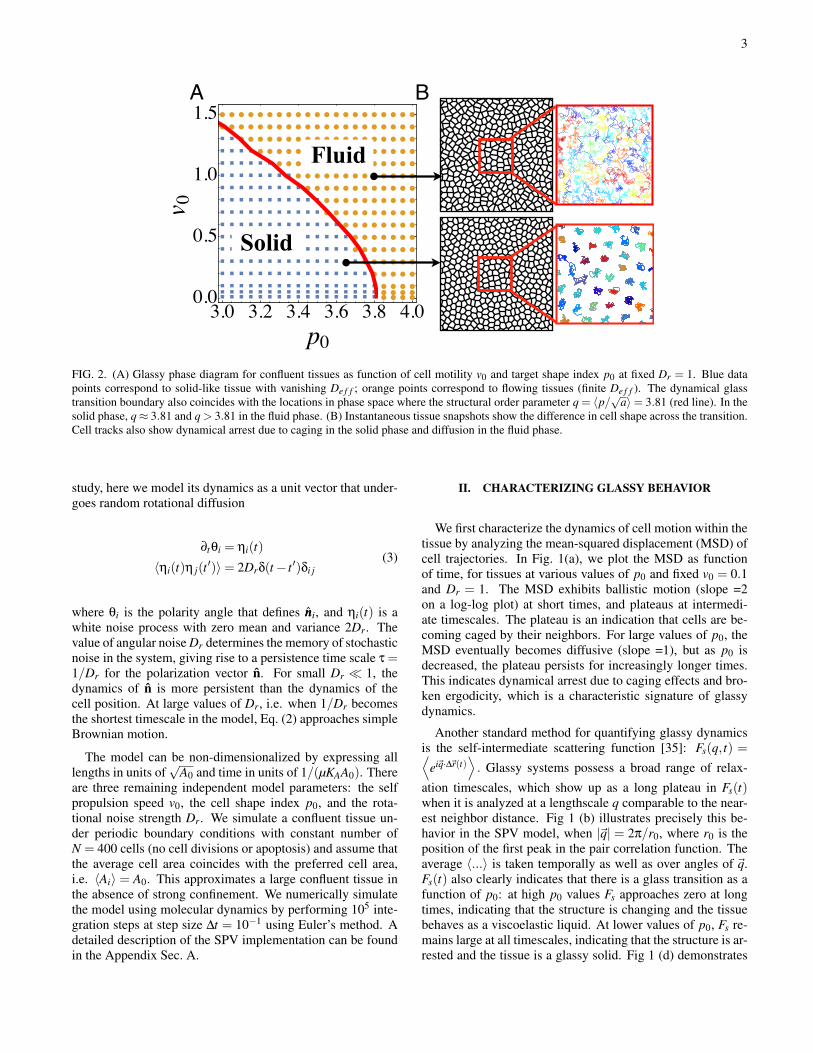
firmed by preliminary explicit calculation of cellular stressesand pressure in the SPV model [43]. This suggests that onemay estimate cell motility by examining the changes in cel-lular stresses and pressure in the cell monolayer near the un-jamming transition and assuming that the local velocity of themonolayer is very small just above the transition. The latterassumption can also be verified independently via particle im-age velocimetry (PIV).

Another result of this work is the surprising and unexpecteddifferences between confluent models (such as the vertex andSPV models) and particle-based models (such as Lennard-Jones glasses and SPP models). For example, works byBerthier [20], Fily and Marchetti in SPP models suggest thatthe location of the zero motility glass transition packing den-sity φG (defined as the density at which dynamics cease in thelimit of v0→ 0) depends the value of noise, Dr. This is also re-lated to the observation that the jamming and glass transitionare not controlled by the same critical point in non-active sys-tems [44, 45]. We find this is not the case in the SPV model.Fig. 3(a & b) show that while the glass transition point p∗0shifts with Dr at finite values of v0, in the limit of vanishingmotility, all glass transition lines merge on to a single point inthe limit v0→ 0, namely p∗0 = 3.81.

Given these differences, it is important to ask which typeof model is appropriate for a given system. We argue thatSPV models are may be more appropriate for many biologicaltissues. Whereas SPP models interact with two-body interac-tions that only depend on particle center positions, both SPVand vertex models capture more information because they takeinto account the intercellular forces due to shape deforma-tions that are inherently multi-body interactions. Unlike ver-tex models, SPV models account for cell motility, and they arealso much easier to simulate in 3D (which is nearly impossiblein practice for the vertex model.)

In our version of the SPV model, we have assumed that cellpolarity is controlled by simple rotational white noise. It isalso possible to include more complex mechanisms. For ex-ample, external chemical or mechanical cues could be mod-eled by coupling v0 and nnni to chemoattractant or mechanicalgradients, allowing waves or other pattern formation mecha-nisms to interact with the jamming transition. Similarly, sim-ple alignment rules (such as those in the Viscek model [46])could lead to collective flocking modes that also affect glassydynamics. These are interesting areas for future research.

Another interesting extension of the SPV model would beto study the role of cell-cell friction. Our current model in-cludes viscous frictional coupling of cell to the 2D substrateand cell-cell adhesion enters as a negative line tension on in-terfaces. However, it would be possible to add a frictionalforce between cells proportional to the length of the edgeshared between two cells, and we know from previous workon particulate glasses that these localized frictions can changethe location of jamming/glass transition and the nature of spa-tial correlations in a glass [47, 48].

In the SPV model, the jamming transition occurs at fixedarea density, which makes it an appropriate model for conflu-ent tissues where there are no spaces between cells. However,it is clear that in many of these tissues, cells change their num-

ber density through cell division, apoptosis, or growth. De-pending on the precise mechanism, changes to number densityalter the ratio between the cell area A0 and the cell perimeterP0, resulting in systematic changes to the model parameterp0. Understanding how p0 changes with cell division, for ex-ample, and making predictions about how tissue solidificationchanges with number density is an interesting avenue for fu-ture research.

It is also tempting to speculate about the relationship be-tween the unjamming transition captured by our model and theepithelial-mesenchimal transition (EMT) that precedes cellescape from a solid tumor mass. The EMT involves significantchanges in cell-cell adhesion and cytoskeletal composition,with associated changes in cell shape and motility. This sug-gests that escape from the tumor mass is controlled not just bythe chemical breakdown of the basement membrane, but alsoby specific changes in mechanical properties of both individ-ual cells and the surrounding tissue. One could then hypoth-esize that the collective unjamming described here may pro-vide the first necessary step towards the mechanical changesneeded for cell escape from primary tumors.

In particular, recent work suggests that cancer tumors aremechanically heterogeneous, with mixtures of stiff and softcells that have varying degrees of active contractility [34]. Ourjamming phase diagram suggests that the soft cells, which of-ten exhibit mesenchymal markers and presumably correspondto higher values of p0, might unjam and move towards theboundary of a primary tumor more easily than their stiff coun-terparts. Examining the effects of tissue heterogeneity on tis-sue rigidity and patterns of cell motility is therefore a verypromising avenue for developing predictive theories for tumorinvasiveness and metastasis.

Appendix A: Simulation algorithm for the SPV model

To create an initial configuration for the simulation, we firstgenerate a seed point pattern using random sequential addi-tion (RSA) [49] and anneal it by integrating Eq. 2 with v0 = 0for 100 MD steps. The resulting structure then serves as aninitially state for all simulations runs. The use of (RSA) onlyserves to speed up the initial seed generation as using a Pois-son random point pattern does not change the results presentedin this paper.

At each time step of the simulation, a Voronoi tesselation iscreated based on the cell centers. The intercellular forces arethen calculated based on shapes and topologies of the Voronoicells (see discussion below). We employ Euler’s method tocarry out the numerical integration of Eq. 2, i.e., at each timestep of the simulation the intercellular forces is calculatedbased on the cell center positions in the previous time step.

In a Delaunay triangulation, a trio of neighboring Voronoicenters define a vertex of a Voronoi polygon. For example inFig. 6, (~ri,~r j,~rk) define the vertex~h3, which is given by

~h3 = α~ri +β~r j + γ~rk, (A1)

8

where the coefficients are given by

α = ‖~r j−~rk‖2(~ri−~r j) · (~ri−~rk)/D

β = ‖~ri−~rk‖2(~r j−~ri) · (~r j−~rk)/D

γ = ‖~ri−~r j‖2(~rk−~ri) · (~rk−~r j)/D

D = 2‖(~ri−~r j)× (~r j−~rk)‖2.

(A2)

~ri

~rj

~rk

~rl~h1

~h2

~h3

~h4

~h5

~h6

~h7

~h8

FIG. 6. Cell centers positions are specified by vectors {~r}. Theyform a Delaunay triangulation (black lines). Its dual is the Voronoitessellation (red lines), with vertices given by {~h}.

In the vertex model, the total mechanical energy of a tissuedepends only on the areas and perimeters of cells:

E =N

∑i=1

[KP(Ai−A0)

2 +KP(Pi−P0)2] . (A3)

In a Voronoi tessellation, the area and perimeter of a cell i canbe calculated in terms of the vertex positions

Pi =zi−1

∑m=0‖~hm−~hm+1‖;

Ai =12

zi−1

∑m=0‖~hm×~hm+1‖,

(A4)

where zi is the number of vertices for cell i (also number ofneighboring cells) and m indexes the vertices. We use the con-vention~hzi =

~h0.With these definitions, the total force on cell-i can be cal-

culated using Eq. A3

Fiµ ≡−∂E∂riµ

=− ∑j∈n.n.(i)

∂E j

∂riµ− ∂Ei

∂riµ, (A5)

here µ denotes the cartesian coordinates (x,y). The first termon the r.h.s. of Eq. A5 sums over all nearest neighbors of celli. It is the force on cell i due to changes in neighboring cellshapes. The second term is the force on cell i due to shapechanges brought on by its own motion.

It maybe tempting to treat ∂E j∂riµ

as the force between cells-iand j, but

∂E j

∂riµ6= ∂Ei

∂r jµ(A6)

since the interaction is inherently multi-cellular in nature andinteractions between i and j also depend on k and l (seeFig. 6).

For the typical configuration shown in Fig. 6, the first termin Eq. A5 can be expanded using the chain rule and calculatedusing Eq. A1

∂E j

∂riµ= ∑

ν

(∂E j

∂h2ν

∂h2ν

riµ+

∂E j

∂h3ν

∂h3ν

riµ

). (A7)

In Eq. A7, only terms involving~h2 and~h3 are kept since E jdoes not depend on other vertices of cell i. ν is a cartesiancoordinate index. The energy derivative in Eq. A7 can be cal-culated in a straightforward way, by using Eqs. A3 and A4

∂E j

∂h2x=2KA(A j−A0)

∂A j

∂h2x+2KP(Pj−P0)

∂Pj

∂h2x

=KA(A j−A0)(h3y−h7y)

+2KP(Pj−P0)

(h2x−h7x

‖~h7−~h2‖+

h2x−h3x

‖~h2−~h3‖

) (A8)

and

∂E j

∂h2y=2KA(A j−A0)

∂A j

∂h2y+2KP(Pj−P0)

∂Pj

∂h2y

=KA(A j−A0)(h3x−h7x)

+2KP(Pj−P0)

(h2y−h7y

‖~h7−~h2‖+

h2y−h3y

‖~h2−~h3‖

).

(A9)

Similarly, the second term on the r.h.s. of Eq. A5 can be cal-culated in a similar way.

Appendix B: Cell displacements and structural order parameteras a function of Dr

1. Expanding cell displacements in an eigenbasis associatedwith the underlying dynamical matrix

In the absence of activity (v0 = 0), the tissue is a solidfor p0 < p∗0 = 3.81. As v0 is increased, the solid behaviorpersists up to v0 = v∗0(p0), which is given by the glass tran-sition line in Fig. 2. In order for the tissue to flow, suffi-cient energy input is needed to overcome energy barriers inthe potential energy landscape, which are a property of theunderlaying solid state at v0 = 0. In this limit, the instan-taneous cell center positions {~ri(t)} can be thought of as asmall displacement {~di(t)} from the nearest solid referencestate {~r0i} [17] where ~di(t) =~ri −~r0i. The ~r0i correspondto positions of cell in a solid, which has a well-defined lin-ear response regime [23]. The linear response is most con-veniently expressed as the eigen-spectrum of the dynamicalmatrix Di jαβ. Since the eigenvectors {ei,ν} of Di jαβ form acomplete orthonormal basis, the cell center displacement canthen be expressed as a linear combination of {ei,ν}

~di(t) = ∑ν

aν(t)ei,ν (B1)

9

For simplicity, we will adopt the Bra-ket notation and expressthe eigenbasis simply as |ν〉 and Eq. B1 becomes

|d〉= ∑ν

aν(t)|ν〉, (B2)

where

D|ν〉= ω2ν|ν〉 (B3)

and ω2ν are the eigenvalues of the dynamical matrix.

The polarization vector ni can also be expressed as a linearcombination of eigenvectors

|n〉= ∑ν

bν(t)|ν〉. (B4)

Since the polarization vector and eigenvector are both unitvectors, it follows that bν(t) = 〈n|ν〉= cos(θν−ψ). Where ψ

is the angle of the polarization and θν the angle of the eigen-vector.

Then the equation of motion for ~di (Eq. 2), can be rewrittenas

~d =−µ∂E∂~ri

∣∣∣∣~r0,i

+ v0ni (B5)

Using Eqs. B2–B5, we find

ddt〈ν|d〉=−µ〈ν|D d〉+ v0〈ν|n〉 ,or

ddt

aν(t) =−µω2νaν(t)+ v0bν(t).

(B6)

Then the equation of motion for each amplitude is

ddt

aν(t) =−µω2νaν(t)+ v0cos(θν−ψ)

ψ = η.(B7)

This is just the equation of motion for a self-propelled particletethered to a spring with active forcing that is strongest alongthe direction of the eigenvector. The solution is then:

aν(t) = aν(t = 0)e−kt + v0

∫ t

0dt ′e−k(t−t ′)cos(θν−ψ), (B8)

where k = µω2ν.

Solving for the ensemble averaged quantity:

〈aν(t)〉= aν(t = 0)e−kt +v0

ξ

∫ t

0dt ′e−k(t−t ′)〈cos(θν−ψ)〉,

(B9)and using the relations

〈cosψ(t)〉= cosψ(0)e−Drt ;

〈sinψ(t)〉= sinψ(0)e−Drt

cos(θν−ψ) = sin(θν)sin(ψ)+ cos(θν)cos(ψ),

(B10)

to get the ensemble averaged solution for the amplitude be-comes

〈aν(t)〉= aν(0)e−kt +v0

ξcos(θν−ψ(0))

e−kt − e−Drt

Dr− k.

(B11)In the Brownian limit Dr→ ∞ and Eq. B11 becomes

〈aν(t)〉= aν(0)e−kt +v0

ξcos(θν−ψ(0))

e−Drt

Dr. (B12)

This suggests that while normal modes control the rate of de-cay, they do no addect the long-time behavior.

However as Dr→ 0, Eq. B11 becomes

aν(t) = aν(0)e−µω2νt +

v0

µω2ν

cos(θν−ψ(0))(

1− e−µω2νt)

(B13)The second term in this equation scales as∼ 1/ω2

ν. Therefore,at short times (corresponding to instantaneous response), themode amplitude aν is much larger for modes at lower frequen-cies. Since the reference state is an elastic solid with Debyescaling D(ω) ∼ ω as ω→ 0 [23], this suggests that the dis-placement will be heavily dominated by the lowest frequencymodes that are spatially more collective in nature.

2. Effect of Dr on glass transition boundary

■ ■ ■ ■ ■ ■ ■ ■ ■ ■ ■ ■ ■ ■ ■ ■ ■

■ ■ ■ ■ ■ ■ ■ ■ ■ ■ ■ ■ ■ ■ ■ ■ ■

■ ■ ■ ■ ■ ■ ■ ■ ■ ■ ■ ■ ■ ■ ■ ■

■ ■ ■ ■ ■ ■ ■ ■ ■ ■ ■ ■ ■ ■ ■

■ ■ ■ ■ ■ ■ ■ ■ ■ ■ ■ ■ ■ ■

■ ■ ■ ■ ■ ■ ■ ■ ■ ■ ■ ■ ■

■ ■ ■ ■ ■ ■ ■ ■ ■ ■ ■ ■

■ ■ ■ ■ ■ ■ ■ ■ ■ ■

■ ■ ■ ■ ■ ■ ■ ■ ■

■ ■ ■ ■ ■ ■ ■

■ ■ ■ ■ ■ ■

● ● ● ●

● ● ● ●

● ● ● ● ●

● ● ● ● ● ●

● ● ● ● ● ● ●

● ● ● ● ● ● ● ●

● ● ● ● ● ● ● ● ●

● ● ● ● ● ● ● ● ● ● ●

● ● ● ● ● ● ● ● ● ● ● ●

● ● ● ● ● ● ● ● ● ● ● ● ● ●

● ● ● ● ● ● ● ● ● ● ● ● ● ● ●

��� ��� ��� ��� ��� ������

���

���

���

���

���

��

� �

■ ■ ■ ■ ■ ■ ■ ■ ■ ■ ■ ■ ■ ■ ■ ■ ■ ■■ ■ ■ ■ ■ ■ ■ ■ ■ ■ ■ ■ ■ ■ ■ ■ ■ ■

■ ■ ■ ■ ■ ■ ■ ■ ■ ■ ■ ■ ■ ■ ■ ■ ■

■ ■ ■ ■ ■ ■ ■ ■ ■ ■ ■ ■ ■ ■ ■ ■ ■

■ ■ ■ ■ ■ ■ ■ ■ ■ ■ ■ ■ ■ ■ ■ ■ ■

■ ■ ■ ■ ■ ■ ■ ■ ■ ■ ■ ■ ■ ■ ■ ■ ■

■ ■ ■ ■ ■ ■ ■ ■ ■ ■ ■ ■ ■ ■ ■ ■

■ ■ ■ ■ ■ ■ ■ ■ ■ ■ ■ ■ ■ ■ ■ ■

■ ■ ■ ■ ■ ■ ■ ■ ■ ■ ■ ■ ■ ■ ■

■ ■ ■ ■ ■ ■ ■ ■ ■ ■ ■ ■ ■ ■ ■

■ ■ ■ ■ ■ ■ ■ ■ ■ ■ ■ ■ ■ ■

● ● ●● ● ●

● ● ● ●

● ● ● ●

● ● ● ●

● ● ● ●

● ● ● ● ●

● ● ● ● ●

● ● ● ● ● ●

● ● ● ● ● ●

● ● ● ● ● ● ●

��� ��� ��� ��� ��� ������

���

���

���

���

���

��

� �

■ ■ ■ ■ ■ ■ ■ ■ ■ ■ ■ ■ ■ ■ ■ ■ ■■ ■ ■ ■ ■ ■ ■ ■ ■ ■ ■ ■ ■ ■ ■ ■ ■■ ■ ■ ■ ■ ■ ■ ■ ■ ■ ■ ■ ■ ■ ■ ■ ■

■ ■ ■ ■ ■ ■ ■ ■ ■ ■ ■ ■ ■ ■ ■ ■

■ ■ ■ ■ ■ ■ ■ ■ ■ ■ ■ ■ ■ ■ ■

■ ■ ■ ■ ■ ■ ■ ■ ■ ■ ■ ■ ■ ■

■ ■ ■ ■ ■ ■ ■ ■ ■ ■ ■ ■ ■ ■

■ ■ ■ ■ ■ ■ ■ ■ ■ ■ ■ ■ ■

■ ■ ■ ■ ■ ■ ■ ■ ■ ■ ■

■ ■ ■ ■ ■ ■ ■ ■ ■ ■ ■

■ ■ ■ ■ ■ ■ ■ ■ ■

■ ■ ■ ■ ■ ■ ■ ■

● ● ● ●● ● ● ●● ● ● ●

● ● ● ● ●

● ● ● ● ● ●

● ● ● ● ● ● ●

● ● ● ● ● ● ●

● ● ● ● ● ● ● ●

● ● ● ● ● ● ● ● ● ●

● ● ● ● ● ● ● ● ● ●

● ● ● ● ● ● ● ● ● ● ● ●

● ● ● ● ● ● ● ● ● ● ● ● ●

��� ��� ��� ��� ��� ������

���

���

���

���

���

��

� �

Dr = 0.01 Dr = 1 Dr = 100

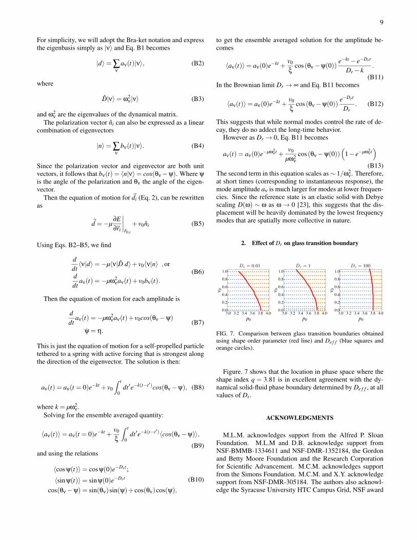
FIG. 7. Comparison between glass transition boundaries obtainedusing shape order parameter (red line) and De f f (blue squares andorange circles).

Figure. 7 shows that the location in phase space where theshape index q = 3.81 is in excellent agreement with the dy-namical solid-fluid phase boundary determined by De f f , at allvalues of Dr.

ACKNOWLEDGMENTS

M.L.M. acknowledges support from the Alfred P. SloanFoundation. M.L.M and D.B. acknowledge support fromNSF-BMMB-1334611 and NSF-DMR-1352184, the Gordonand Betty Moore Foundation and the Research Corporationfor Scientific Advancement. M.C.M. acknowledges supportfrom the Simons Foundation. M.C.M. and X.Y. acknowledgesupport from NSF-DMR-305184. The authors also acknowl-edge the Syracuse University HTC Campus Grid, NSF award

10

ACI-1341006 and the Soft Matter Program at Syracuse Uni- versity.

[1] E.-M. Schoetz, M. Lanio, J. A. Talbot, and M. L. Manning, J.Roy. Soc. Interface 10, 20130726 (2013).

[2] E.-M. Schoetz, R. D. Burdine, F. Julicher, M. S. Steinberg, C.-P.Heisenberg, and R. A. Foty, HFSP journal Vol.2 (1), 1 (2008).

[3] T. E. Angelini, E. Hannezo, X. Trepat, J. J. Fredberg, and D. A.Weitz, Phys. Rev. Lett. 104, 168104 (2010).

[4] T. E. Angelini, E. Hannezo, X. Trepat, M. Marquez, J. J. Fred-berg, and D. A. Weitz, Proceedings of the National Academyof Sciences 108, 4714 (2011).

[5] K. D. Nnetu, M. Knorr, J. Kas, and M. Zink, New Journal ofPhysics 14, 115012 (2012).

[6] J. P. Thiery, Nat Rev Cancer 2, 442 (2002).[7] E. W. Thompson and D. F. Newgreen, Cancer Research 65,

5991 (2005).[8] N. Gunasinghe, A. Wells, E. Thompson, and H. Hugo, Cancer

and Metastasis Reviews 31, 469 (2012).[9] Y. Nakaya, S. Kuroda, Y. T. Katagiri, K. Kaibuchi, and Y. Taka-

hashi, Developmental Cell, Developmental Cell 7, 425 (2015).[10] J.-A. Park, J. H. Kim, D. Bi, J. A. Mitchel, N. T. Qazvini,

K. Tantisira, C. Y. Park, M. McGill, S.-H. Kim, B. Gweon,J. Notbohm, R. Steward Jr, S. Burger, S. H. Randell, A. T. Kho,D. T. Tambe, C. Hardin, S. A. Shore, E. Israel, D. A. Weitz,D. J. Tschumperlin, E. P. Henske, S. T. Weiss, M. L. Manning,J. P. Butler, J. M. Drazen, and J. J. Fredberg, Nat Mater 14,1040 (2015).

[11] M. Sadati, N. T. Qazvini, R. Krishnan, C. Y. Park, and J. J.Fredberg, Differentiation 86, 121 (2013), mechanotransduc-tion.

[12] A. Haeger, M. Krause, K. Wolf, and P. Friedl, Biochimica etBiophysica Acta (BBA) - General Subjects 1840, 2386 (2014),matrix-mediated cell behaviour and properties.

[13] A. J. Liu and S. R. Nagel, Annual Review of Condensed MatterPhysics 1, 347 (2010).

[14] V. Trappe, V. Prasad, L. Cipelletti, and P. Segre. . . , Nature(2001).

[15] B. Szabo, G. J. Szollosi, B. Gonci, Z. Juranyi, D. Selmeczi, andT. Vicsek, Phys. Rev. E 74, 061908 (2006).

[16] J. M. Belmonte, G. L. Thomas, L. G. Brunnet, R. M. C.de Almeida, and H. Chate, Phys. Rev. Lett. 100, 248702(2008).

[17] S. Henkes, Y. Fily, and M. C. Marchetti, Phys. Rev. E 84,040301 (2011).

[18] Y. Fily and M. C. Marchetti, Phys. Rev. Lett. 108, 235702(2012).

[19] R. Ni, M. A. C. Stuart, and M. Dijkstra, Nat Commun 4 (2013).[20] L. Berthier, Physical Review Letters 112, 220602 (2014).[21] Y. Fily, S. Henkes, and M. C. Marchetti, Soft Matter 10, 2132

(2014).[22] J. H. Kim, X. Serra-Picamal, D. T. Tambe, E. H. Zhou, C. Y.

Park, M. Sadati, J.-A. Park, R. Krishnan, B. Gweon, E. Millet,J. P. Butler, X. Trepat, and J. J. Fredberg, Nat Mater 12, 856(2013).

[23] D. Bi, J. H. Lopez, J. M. Schwarz, and M. L. Manning, Nat

Phys advance online publication, (2015).[24] T. Nagai and H. Honda, Philosophical Magazine Part B 81, 699

(2001).[25] R. Farhadifar, J.-C. Roeper, B. Aigouy, S. Eaton, and

F. Julicher, Current Biology 17, 2095 (2007).[26] L. Hufnagel, A. A. Teleman, H. Rouault, S. M. Cohen, and B. I.

Shraiman, Proceedings of the National Academy of Sciences104, 3835 (2007).

[27] D. B. Staple, R. Farhadifar, J. C. Roeper, B. Aigouy, S. Eaton,and F. Julicher, Eur. Phys. J. E 33, 117 (2010).

[28] M. L. Manning, R. A. Foty, M. S. Steinberg, and E.-M.Schoetz, Proceedings of the National Academy of Sciences107, 12517 (2010).

[29] D. Bi, J. H. Lopez, J. M. Schwarz, and M. L. Manning, SoftMatter 10, 1885 (2014).

[30] B. Li and S. X. Sun, Biophysical Journal, Biophysical Journal107, 1532 (2015).

[31] A. Szabo, Runnep, E. Mehes, W. O. Twal, W. S. Argraves,Y. Cao, and A. Czirok, Physical Biology 7, 046007 (2010).

[32] A. J. Kabla, Journal of The Royal Society Interface 9, 3268(2012).

[33] G. Lejeune Dirichlet, Journal fur die reine und angewandteMathematik 40, 209 (1850).

[34] F. Wetzel, A. Fritsch, D. Bi, R. Stange, S. Pawlizak, T. Kieβling,L.-C. Horn, K. Bendrat, M. Oktay, M. Zink, A. Niendorf,J. Condeelis, M. Hockel, M. C. Marchetti, M. L. Manning, andJ. K. Kas, Unpublished (2015).

[35] L. Van Hove, Phys. Rev. 95, 249 (1954).[36] N. Xu, V. Vitelli, A. J. Liu, and S. R. Nagel, EPL (Europhysics

Letters) 90, 56001 (2010).[37] M. L. Manning and A. J. Liu, Phys. Rev. Lett. 107, 108302

(2011).[38] C. Monthus and J.-P. Bouchaud, Journal of Physics A: Mathe-

matical and General 29, 3847 (1996).[39] P. Sollich, Phys. Rev. E 58, 738 (1998).[40] A. R. Abate and D. J. Durian, Phys. Rev. Lett. 101, 245701

(2008).[41] F. Cecconi, A. Puglisi, U. M. B. Marconi, and A. Vulpiani,

Phys. Rev. Lett. 90, 064301 (2003).[42] D. L. Weaire and S. Hutzler, The physics of foams (Oxford Uni-

versity Press, 1999).[43] X. B. Yang, D. Bi, M. C. Marchetti, and M. L. Manning, Un-

published (2015).[44] A. Ikeda, L. Berthier, and P. Sollich, Phys. Rev. Lett. 109,

018301 (2012).[45] P. Olsson and S. Teitel, Phys. Rev. E 88, 010301 (2013).[46] T. Vicsek, A. Czirok, E. Ben-Jacob, I. Cohen, and O. Shochet,

Phys. Rev. Lett. 75, 1226 (1995).[47] L. E. Silbert, Soft Matter 6, 2918 (2010).[48] S. Henkes, M. van Hecke, and W. van Saarloos, EPL (Euro-

physics Letters) 90, 14003 (2010).[49] S. Torquato, Author and H. Haslach, Jr, Applied Mechanics Re-

views 55, B62 (2002).