Mothers in an insider-outsider economy: The puzzle of Spain

J Popul Econ (1996) 9:301-323 --dournaJ o f - -

population Economics © Springer-Verlag 1996

Mothers in an insider-outsider economy: The puzzle of Spain

Paula Adam 1,2

1 Department of Economics, European University Institute, 1-50016 San Domenico di Fiesole, Italy 2IGIER, Via Salasco 5, 1-20136 Milano, Italy (Fax: +39258363302; e-mail: [email protected])

Received January 15, 1996 / Accepted June 18, 1996

Abstract. There is growing evidence tha t social policies towards mothers have i m p o r t a n t effects on their l abour marke t behaviour . This ar t ic le argues tha t these effects are less i m p o r t a n t in a Male Breadwinner Regime if there is emp loymen t insecur i ty in the househo ld or i f women in tend to pa r t i c ipa te in the long-run . I cons ider the case o f Spain, where the workforce has become po la r i zed between insiders and outs iders and where social policies closely resemble the Male Breadwinner Regime. The results show tha t Spanish mothe r s fall in to two groups: those who do not wi thdraw f rom the l abo r force af ter ch i ldb i r th and those who wi thdraw and do no t re-enter af ter thei r chi ldren arrive at school age. En t ry or re-entry appears re la ted to the hus- b a n d ' s emp loymen t uncer ta inty. M a r r i e d women in an " ins ider househo ld" are less l ikely to be mobi le than women in an "ou ts ider househo ld" .

J E L classification: J 22, J 13

Key words: Chi ldb i r th , l abor force pa r t i c ipa t ion , l abo r force t rans i t ions

This research was initiated with the financial support from the Bank of Spain (Fondo para Estudios sobre el Mercado de Trabajo) and the CIRIT (Generalitat de Catalunya). An earlier version has been published in Spanish in Adam, 1995a. I benefited from presentations in the session on Women's Labour Force Transitions in the ESPE ninth annual meeting at Lisbon, in the IESA (CSIC, Madrid) seminar, in the session on European Labour Markets in the IEA meeting at Tunis, and in the IGIER seminar. I thank Namkee Ahn, Sir Gustafsson, John Er- misch, Andrea Ichino, Sergi Jim6nez, Dennis Snower, Robert Waldmann and an anonymous referee for comments. My very especial thanks go to my thesis supervisor, John Micklewright, to Gosta Esping-Andersen, John Myles and David Soskice. Responsible editors: Siv S. Gustafsson, John E Ermisch.

302

1. Introduction

P. Adam

There is growing evidence that childcare and maternity leave provisions have a positive impact on married women's labour force participation. Gustafsson and Stafford (1994) distinguish two policy models: the traditional Male Breadwinner Model which encourages women to withdraw from the labour force after childbirth, and the Individual Model which encourages female re- entry. This difference has been studied in several comparative analyses ap- plied to US and Northern European countries (see Gustafsson and Stafford 1994; Gustafsson et al. 1996; Ondrich et al. 1996; ROnsen and SundstrOm 1996). The central point of this article is that the behaviour of women subject to "male breadwinner" policies may not be as expected when unemployment and job insecurity among "male breadwinners" is high.

Insider-outsider economies are ideal to investigate this issue. The polarization of the labour force in these economies is often reflected through the levels of labour force rotation and mobility: insiders (with high employment security) usually enjoy lung tenure, while outsiders (with low employment security) often shift between intermittent episodes of employment and unemployment. In this context, "male breadwinner" policies are likely to be less effective among outsider households: women may compensate for the household's employment uncertainty, probably with intermittent episodes as well. Among insider households, the response of highly educated mothers to "male breadwinner regimes" may not be as expected if women study because they intend to participate over the entire life-cycle. Highly educated women usually have high real wages which allow dual earner households to afford alternative sources of child care.

Spain is a suitable case to investigate this issue. Its design of social policies towards working mothers resembles closely the breadwinner model in the sense that women are not encouraged to return to work after maternity leave. However, in Spain employment is not guaranteed for a significant proportion of the population. On the one hand, male, female and youth unemployment rates are the highest among OECD countries and, on the other hand, job stability has become highly polarized since the early 1980s between insiders (with permanent contracts) and outsiders (with fixed term contracts). In this context, one would expect the "male breadwinner" policies to be more effective among wives in insider households, than among wives inserted in households with weak job guarantees.

This article is organized as follows. In Section 2 I describe the recent trends in female labour participation in Spain. Section 3 examines the Spanish "Male Breadwinner Regime" comparatively. Section4 describes employment and unemployment trends, and the institutional factors that have favored an insider-outsider polarization in Spain. Section 5 is devoted to the empirical model and its interpretation. Section 6 describes the empirical results, and Section 7 concludes.

2. Female labour force participation

Traditionally, female labour force participation in Spain has been among the lowest in the OECD. Participation has risen since the 1970s by an annual av-

Mothers in an insider-outsider economy 303

erage of 0.4 percentage points, which is lower than in other OECD countries. Nevertheless, in the mid 1980s the growth in female labour force participation has been substantial. Between 1985 and 1992, it rose from 34.8% to 43.6°7o (e.g. an annual average increase of 1.3 points). This increase is more striking among young population groups (excluding those in education, aged < 25). Indeed, for the age group 25- 49 participation rates increased 6.3 percentage points (on average) from 1984 to 1992. Had all entering women actually found jobs, they would have absorbed 70°7o of all job creation. This occurred during a period when the average unemployment rate was around 20%.

Some authors conclude that this female participation growth has been promoted by cyclical effect (encouraged worker effect), given the great employment creation during the second half of the 1980s (see Novales 1989; Albarracin and Artola 1989; Novales and Mateos 1990). However, there are indications that long term secular trends may be even more important (see Adam 1995b). The large increase in female participation in the 1980s was ac- companied by: (i) a structural change in the demand for labour which favored female employment; and (ii) a change in women's life-cycle behaviour, reflected in delayed entry into the labour market due to human capital invest- ment, in higher participation rates after marriage and childbirth, and in decreasing fertility. The key piece of evidence is Arellano and Bover's (1995) time series estimation. Although they find a significant business cycle effect, they conclude that the main effect is due to structural shifts in female earnings potential. Given these results, the predictions of Arellano and Bover are that: " [ . . . ] the levels of prime age female participation that have been reached and that were never experienced before are here to stay. Even if these levels remained constant in the future, we wouM expect the total participation rate to increase due to the replacement of the older cohorts" (1995, pp. 188-189).

Despite the new life-cycle participation profile (especially among highly educated women) and the increase in participation among younger cohorts, female participation rates are still the lowest among OECD countries. This suggests that there is one group of women who a priori intend not to work; I shall call these a priori non-participating women in the case that they do participate. Another group of women intends to remain permanently employed. This group I will call long-run participants. This distinction is used in this research to examine: (i) the response to the "male breadwinner regime", and (ii) the response to husband's employment situation within these two different groups of women.

3. The Spanish male breadwinner regime

Table 1 shows that in countries with different childcare and parental leave regimes 1 mothers' employment rates differ sharply by age of youngest child. In Sweden there is an extensive program of universal daycare and maternity leave (65 weeks). In the United States there is very little public support for child care (except for tax credits that mainly benefit lower-middle income groups) and no paid or unpaid parental leave. As a result, Swedish women tend to re-enter the labour force after maternity leave, while American

304 P. Adam

Table 1. Employment rates (%) of mothers by age of youngest child in selected OECD countries

Age of youngest Sweden a United States b Netherlands c Spain d child

< 1 41.3 42.4 25.7 23.7 1 79.6 54.8 22.1 30.9 e 2 - 3 76.2 55.6 26.8 20.1 f 4 - 5 75.0 63.1 37.9 -

>6 83.4 g - 34.89 h 9.9

Source: Gustafsson S, Stafford F (1994) (Tables 11.3, 11.5, 11.6, pp 349-350), and my own calculations. Note: The source of the Spanish figures in the ECPF (pooled sample), 1985- 90. a Women's age 18-64 as of 1984. b Women's age 23- 30 as of 1988. c Women's age 16-65 as of 1988. a Married women, all age groups. e Youngest child aged 1 - 2. f Youngest child aged 3 - 5. g Youngest child aged > 6. h Youngest child aged 6-18.

mothe r s tend to re turn to work immed ia t e ly af ter ch i ldbi r th . The employ- men t rate a m o n g Swedish mo the r s wi th chi ldren under age 1 is a lmos t 40 percentage po in t s lower t han a m o n g women with o lder preschoolers , while in the Uni ted States it is on ly a b o u t 10 po in t s lower.

In the Ne ther lands , m a t e r n i t y leave provis ion provides 100%0 of the previous wage for 16 weeks and there is no subs tan t ia l daycare provis ion. Thus, the di f ference in e m p l o y m e n t rates o f w o m e n with the younges t child less t han one and more t han one is less than 5 points . The lack o f subs tan t ia l daycare seems to affect exper ience loss, ref lected in the e m p l o y m e n t rates o f mo the r s wi th school age chi ldren: once the younges t chi ld arr ives at school age, e m p l o y m e n t rate a m o n g Swedish mo the r s increases a lmos t 10 points , while a m o n g Du tch mothe r s it decreases by 3 points .

Despi te (op t iona l ) separa te income t axa t ion in the househo ld since 1988, Spa in lies close to the Male Breadwinner Mode l . Ma te rn i t y benef i t s provide 75% o f previous wages for 14 weeks. 2 Af t e r the first three m o n t h s there is no n a t i o n a l pol icy and daycare services are very l imi ted ( including local com- mune daycare) . Despi te the lack o f substant ive daycare provis ion, this does no t reduce the incentives for w o m e n with pre -school chi ldren to enter the l abou r force. Moreover, previous ly employed mothe r s do make use o f mater - n i ty leave. Seventeen percent o f mo the r s wi th one child less than 3 m o n t h s are at work c o m p a r e d to 23.3o70 o f mothe r s wi th one chi ld aged 4 - 1 2 mon ths (Spanish I n c o m e and Expend i tu res Survey, ECPF, poo l ed d a t a 1985 -90 ) .

Once the chi ldren arr ive at school age (6 years), the incentives for Span ish mo the r s to re turn to work are not very s t rong even i f school ing is c o m p u l s o r y and free o f charge. O n the one hand , a l t hough the Span ish school day is usua l ly long (8 hours per day, f rom 9 a m to 5 pm) this still poses an obstacle for women to re turn to work because, unl ike in o ther O E C D countr ies , par t - t ime cont rac ts are rare (see O E C D 1994). On the o ther hand , the loss o f exper ience dur ing ma te rn i t y absence might be qui te s ignif icant . However, even


if the Spanish childcare regime is similar to that of the Netherlands, differences in employment rates by age of youngest child differ tremendously between mothers of school-age children and those with oder pre-schoolers.

The different pattern of mothers' employment in Spain compared to other countries with similar regimes suggests the existence of other factors which influence Spanish mothers' behaviour. On the one hand, a cohort effect (reflected through the age of youngest child) may partly dictate Spanish mothers' behaviour. In fact, mothers with the youngest child less than one belong to the 1960 cohort (on average), while mothers with the youngest child aged 1-3 , aged 3 - 6 and aged >6 belong respectively to the 1955 cohort, the 1940 cohort and the 1930 cohort (on average). On the other hand, as I describe in the following section, the costs of prolonged labour market absence may be especially high in an "insider-outsider" economy like the Spanish.

4. Employment and unemployment, insiders and outsiders

Female unemployment in Spain is very high: 28% in •987 and 24°70 in 1990 (according to the labour Force Survey, which is a more optimistic source than the Employment Office data bank). In spite of the scarcity of part-time female work, 3 atypical employment is now widespread in the form of temporary contracts (i.e. fixed-term contracts with low firing costs, only renewable through permanent contracts) as a result of new legislation introduced in 1984. The proportion of female "temporaries" rose from 18.4°70 of female wage employment in 1987 to 34.2% in 1990, the highest level in the OECD area. Because of expected long periods of absenteeism employers are more likely to favor temporary over permanent contracts for women. The result is a large increase in female labour rotation.4

But temporary contracts are also widespread among (young and adult) men. The debate in the Spanish economic literature about the implications of the extensive use of temporary contracts focuses mainly on its impact on wage setting, and on access to stable employment. It is often concluded that temporary contracts have introduced more rigidity to the system because they create more stability and bargaining power for the permanent workers, and more job volatility within the rest of the population (Bentolila and Dolado 1994; Jimeno and Toharia 1993). Indeed, before 1984 Spain had the longest average job tenure in the OECD, and short term rotation levels were below the OECD average. Seven years later, average tenure remains among the longest in the OECD, but the percentage of workers with less than one year's tenue has, concomitantly, grown tremendously. This, in combination with high unemployment, is consistent with the argument that the Spanish workforce has polarized into an insider and outsider group in terms of access to stable employment and job security (see Lindbeck and Snower 1988). Revenga (1994) describes the existence of a bimodal distribution, with a large number of workers enjoying long tenure (18.4% have more than 20 years tenure) and a growing number of workers with short term turnover (rising from 15070 in 1987 to 24% in 1991). Although the increase of workers with brief tenure may also be due to the recent inflow of new workers, the relationship between the implementation of temporary contracts and employment

306 P. Adam

rotation is clear: only 17% of temporary workers in any year made a transition to permanent contracts 1 year later (Segura et al. 1991). Given the temporary contracts cannot be renewed with another temporary contract by law (AES), this often implies a transition to unemployment. Moreover, before 1992 temporary workers were entitled to unemployment benefit for up to half time of their tenure with a tax-free benefit equal to 80% of previous salary. This gave incentives to some workers to search for short term jobs, followed by intermittent episodes of unemployment (see Bentolila and Dolado 1994). 5 Therefore, temporary contracts seem to be the main cause of the increased labour rotation with intermittent employment among the outsiders.

Within households, the dualisation of the Spanish labour market during the second half of the 1980s has introduced employment uncertainty. If married women are sensitive to the labour and income expectations of the household, they may accept paid jobs to compensate for household uncertainty. Two factors suggest that these are likely to be unstable jobs. One, outsider household breadwinners are likely to be inserted in environments with weak labour market networks, which therefore lowers the probability that the wife finds a stable and/or insider job. Two, household work is usually carried out by wives, and finding substitutes often implies high costs. Therefore, if women combine household and market work, their available time often restricts them to irregular jobs, i.e. high rotation. In this case, women will complement the mobility of other household members with their own mobility. These women are active on the margin because they keep a marginal at- tachment to the labour force, typically characterized by intermittent episodes of employment and inactivity, usually as a response to fluctuations in husband's employment and income. Thus, the labour force rotation of married women may very well be due to a compensation and cyclical effect.

To conclude, married women's mobility may be the result of two separate forces, one which is distinct for long-term participating women, another for short term participating women. In the first case, turnover of a priori active women (usually with high education) should be similar to men, although there are differences when it comes to aspects such as maternity (which also affects mobility). In the second case, mobility of a priori inactive women living in households with an "outsider" breadwinner may have increased in tandem with the increasing polarization of the Spanish workforce.

5. The empirical model

5.1 The standard participation probability model

Let us assume a linear participation function in reduced form g = aXi t+bZi+u i t for wife i at time t, i = 1 . . . . . N , t = 1 . . . . T, where a and b are parameters. The observed vectors of time-variant variables )(it and time-invariant variables Z i are assumed to be exogenous and include factors that affect the reservation wage and market wage values of wife i at time t (see Deaton and Muellbauer 1984). The error term uit includes the unobserved time-variant and time-invariant factors. Typically, the reservation wage value depends on factors such as tastes for use of non-market time, fixed costs of participation such as childcare, wife's individual characteristics, household non-labour income, husband's earnings, etc. The market


wage value depends on factors that determine wives's expected salary in the current labour market, such as wife's education and labour market experience, a given policy she faces, the regional price index, and other economic indicators such as the local unemployment rate.

Let us assign values 0 and 1 to the two possible labour market states (participation and non-participation in the labour force), and define a sequence of binary random variables:

I 1 if i-th wife participates at time t

.Fit = 0 otherwise . (1)

In other words, Yit = ] if g < 0 and Yit = 0 if g--<0. The probabilistic binary choice model can then be defined as follows:

P(Yi = 1 ) = P ( g > 0 ) = G(aXi t+bZi )

P(Yit = 0 ) = P ( g < 0 ) = 1 - P ( g > 0 ) = 1 - G ( a X i t + b Z i ) , (2)

where G is the associated probability distribution of g.

5.2 Transition probabilities

The central objective of this article is to analyze the flow between participation and inactivity for married women in any given period. The essential toot for this analysis is the transition probability. That is, the probability of mov- ing from one labour market state to another during a given time interval. With discrete time data, transition models are a good choice.6 A particular case is the discrete-state, discrete-time Markov model with exogenous variables, which is represented by the parametric analysis of discrete states under the general assumption that an individual' choice of labour market state can be viewed as a first order Markov process. This model is a natural extension of the static qualitative choice model to a dynamic context, where changes in labour market states occur over time as a result of either changes in stochastic characteristics of the individual or the environment, or simply due to individual characteristics which define a mobility propensity.

I shall consider a two-state f irst order Markov model with exogenous variables over T periods as described in Amemyia (1985). The transition probability between state 0 and state 1 can be specified as a conditional probability of the form:

pio~(t) = PLv~ = 1 [y~_~ = o] (3)

and similarly,

P~o(t) = PLv~ = OIy~_l = II ,

which is the conditional probability of transition from state 1 and 0.7 The probabilistic specification showed in (3) can be parametrized by introducing a distribution function which depends upon exogenous variables, and which accounts for heterogeneity and non-stationarity of the data. How to specify

308 P. Adam

this function? Given the probabilistic model in (2), the transition probabilities of (3) can be expressed as:

P~1 (t) = P(aXi ' t + b Zi <- O'aXi't-1 + b Zi>- O ) , (4)

l - G ( a X i , t_ 1 + b Z )

P~o(t) = P(aXi' t +b Zi>-O'aXi't-1 + b Zi <-O)

Cr(aSi, t_ l + b Zi)

which therefore depend on the value of the observed time-variant variables in both periods and on the observed time-invariant characteristics. Equa- tion (4) can be expressed as a linear function in reduced form with a simple distribution function F. The time-variant variables at t - 1 and t are included and measure changes in their values. 8 The time-invariant variables are also included and capture the mobility propensity:

P~ol (t) = F ( a ~ ( X i t - l , X i t ) + flZi) (5)

P~o(t) = F(a* q~(Xit_l,Xit)+ fl* Zi) ,

where a, a*, fl and fl* are vectors of parameters. ~ is a function that measures the changes in the observed time-variant exogenous variables from t - 1 to t. The specification of ~ depends on the nature of each variable.9

The estimation procedure assumes a logistic distribution of F. The likelihood function of the transition model is given by the distribution of the four possible events: stay in, entry, stay out and exit from the labour force. Amemiya (1985) shows that estimation of the present model can be carried out with simple logit models of the two separated hazard rates: the probability of entry (or stay out), and the probability of exit (or stay in) the labour force from t - 1 to t.

Interpretation of the empirical model

I have described a transition model with two probability equations. Transi- tions are modelled from time t - 1 to t. The independent variables are all assumed to be exogenous in the model and measured at time t - 1, i.e. before the transition occurs. The dynamic time-variant variables are measured at time t - 1 and t, i.e. q~(Xit_l,Xit). In principle, these are included in the model separation to capture the effect of changes in these explanatory variables, e.g. husband's change in employment status. Nonetheless, some time- variant variables are also included with a static specification in order to assess which provides the better fit. For example, husband's employment status is introduced as a static variable at time t - 1 , and also as a dynamic variable from t - 1 to t. Moreover, the dynamic specification is tested against lagged measures at time t - 2 and t - l , i.e. q~(Xit_z,Xit_l). The time-invariant effects, Z i, are meant to capture fixed effects with an influence on the transition probabilities.


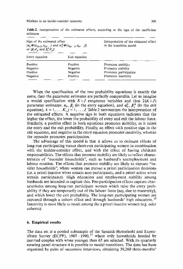
Table 2. Interpretation of the estimated effects, according to the sign of the coefficient estimates

Sign of the estimated effect [ gk ~ (Xkit-2, Xkit - 1 ) a n d a k ~ (Xkit - 2 ' Xkit - 1 )] or bgjZii and/~fZji]

Entry equation Exit equation

Interpretation of the estimated effect in the transition model

Positive Positive Promotes mobility Negative Negative Promotes stability Positive Negative Promotes participation Negative Positive Promotes inactivity

When the specification of the two probability equations is exactly the same, then the parameter estimates are perfectly comparable. ]Let us imagine a model specification with K + J exogenous variables and thus 2 ( K + J ) parameter estimates: a k, pj (in the entry equation), and arc, flJ~ (in the exit equation), k = 1 . . . . K, j = 1 . . . . J. Table 2 summarizes the interpretation of the estimated effects. A negative sign in both equations indicates that the higher the effect, the lower the probability of entry and exit the labour force. Similarly, a positive effect in both equations promotes mobility, as it raises the entry and the exit probability. Finally, an effect with positive sign in the exit equation, and negative in the entry equation promotes inactivity, whereas the opposite promotes participation.

The advantage of this model is that it allows us to estimate effects of long-run participating versus short-run participating women in combination with the insider-outsider effect, and with the effect of having childcare responsabilities. The effects that promote mobility are likely to reflect characteristics of "outsider households", such as husband's unemployment and labour rotation. The effects that promote stability are likely to capture "insider households", where women can pursue a priori participation decisions (i.e. a priori inactive wives remain non-participants, and a priori active wives remain participants). High education and employment stability among husbands are intended to capture this. Pro-participation effects capture characteristics among long-run participant women which raise the entry probability if they are temporarily out of the labour force (say, due to maternity), and which lower the exit probability. The long-run participating women are captured through a cohort effect and through husbands' high education. 10 Inactivity is most likely to result among the a priori inactive women (e.g. oder cohorts).

6. Empirical results

The data set is a pooled subsample of the Spanish Household and Expen- diture Survey (ECPF), 1985-1990, 11 where only households headed by married couples with wives younger than 65 are selected. With its quarterly rotating panel structure it is possible to model transitions. The data has been organized by pairs of successive interviews, obtaining 39,260 three-months'

310 P. Adam

transitions related to 11,802 households. The greatest shortcoming is that there is no information on wives' education, labour market experience and wages, nor on region of residence of the household. Given the great impor- tance of own education and experience for female participation, and the substantial regional differences (in terms of female labour supply behaviour) in Spain, these may well be relevant variables in the model. If the regressors are correlated with the omitted variables, the consequence may be biased parameter estimates. Therefore the goodness of fit of the estimated models is likely to be affected.

The sample transitions are distributed as follows: 24.1°70 of the quarter observations of married women are in the participation pool at time t - 1 . Among these, 8.4% make an exit transition and 91.6% stay at time t. The other 75.9% of quarter observations of married women are in the non-participating pool at time t - 1 . Among these, 3.2% make an entry transition, and 96.8% stay at time t. Table 3 shows the cross-distributions of participation (in %) at time t - 1 and at time t. The off-diagonal cells report the transition rates and the diagonal cells show the survival rates.

The estimation strategy is the following. The same specification is imposed in both the entry and the exit probability equations to obtain perfectly comparable estimates. In terms of goodness of fit of the model, the cost of this strategy is that some irrelevant variables are kept in the specification. Although this does not bias the coefficient estimates, the model loses preci- sion if the irrelevant variables are correlated with other variables in the model specification. The results concerning life-cycle effects are included in Table 4, together with other control variables. Because the time-variation of these variables is trivial, I treat these as time-invariant variables. The effects of children are reported in Table 5, with two different specifications. Again, the time variation of these variables is trivial and therefore these are treated as time-invariant. The exception is the birth of a child. The effects of husbands' labour status (time-invariant specification) are presented in Table 6. Then the effects of husbands' labour market transitions (time-variant specification) are presented in Tables 7 and 8. Descriptive statistics are in the Appendix.

Table 3. Married women ' s labour force transitions in the ECPF pooled subsample

Origin state [time t - 1] Destination state [time t]

Participant Non-part icipant Total

Participant 8, 658 790 29, 812 91.6 8.4 100.0 90.0 2.7 24.1

Non-part icipant 958 28, 854 9, 448 3.2 96.8 100.0

10.0 97.3 75.9

Total 9,616 29,644 39,260 24.5 75.5

100.0 100.0

Note: Cells are organized as normal contingency tables. The first figures (in italics) are the raw numbers . The second are the row percentages and the third are the column percentages.


Transitions over the life-cycle: age and cohort effects. As a first approxima- tion of a life-cycle effect, I examine the effect of age on wives' transitions. A correct specification for wives' age is not straightforward, because the exit rates by wives' age follow a u-curve (reaching around 13% rates in the ex- tremes and 6% as a minimum at the age of 35-39) . This suggests that a quadratic specification would be reasonable. However the entry rates follow a rather decreasing flat curve, suggesting a linear effect. It turns out that linear and quadratic specifications perform poorly when imposed simulta- neously in both equations. I have solved this by using a linear spline function specification because it provides a more flexible alternative to quadratic and linear specifications. 12

The interpretation of the coefficients in the entry equation is the following: a negative sign shows that as age increases, wives are less likely to enter the labour force. 13 As age increases by one year, the entry probability of women aged 3 0 - 4 0 increases 1.5%, while for women aged 4 0 - 5 0 the entry probability decreases 2°-/0 and for women over 50, it decreases 1.7%. Tests for equality of the parameter estimates "wife's age 4 0 - 50" and "wife's age > 50" have not been rejected, which suggests that women have less incentives to enter after the age threshold of 40. Thus, the marginal impacts are quite small and of the same size. What about the size of the effects? These are fairly large 14 and, as discussed later, larger than cohort effects or the impact of husbands' education (except for wives older than 35).

In the exit equation, wives' age parameters are not significant, except "wive's age 3 0 - 4 0 " which is negative. This means that participating wives are less likely to exit at age 40 than at age 30. In this case, the marginalage penalty on the exit probability is 1.9%. The obtained coefficient estimate is not significantly different from the ones obtained in the entry equation. The negative sign in the entry and exit equations suggests the existence of an effect promoting stability, which is larger at age 40 than at age 30. This stability effect is an interesting finding but difficult to interpret without considering other issues related to this period of women's life-cycle. Factors such as cohort membership, childbirth and a greater incidence of fixed-term contracts among women aged 30 than 40 are all likely to play a role. These are discussed below.

Considering the evolution of female participation in Spain, one can expect substantial cohort differences. According to Arellano and Bover (1995), the cohort of 1951 - 6 0 is the first to experience a significant jump in married women's participation rates. In the model specification of Table 4, the dummies capturing 4 different cohorts 15 (the base is: cohort 1921-30) show that, indeed, the 1951-60 and the subsequent cohort (i.e. 196~- 1973) have a large negative coefficient in the exit equation: setting all other effects to zero, being member of the 1951 - 60 cohort (1961 - 73 cohort) lowers the exit probability by 32% (29%) relative to the 1921-30 cohort. Thus, the two effects are significantly not different. Note that older cohorts show no significant effects. Note that these cohorts are aged 2 0 - 4 0 during the years of the ECPF survey (1985 to 1990). Comparing the coefficient estimates, the cohort effect seems to be stronger in reducing the exit probability than the effect of age 20 -40 . The entry probability is clearly not affected by cohort effects, im- plying that differences between younger and older cohorts are not related to entry but to withdrawal from the labour force.

312 E Adam

Table 4. Logit model of transition probabilities: The cohort and age effects, husband's education and district size effects

Entry probability Exit probability (1) (1)

Constant - 3.594 (3.1) - 1.024 (0.8) Wife's age<30 0.055 (1.5) 0.013 (0.3) Wife's age 3 0 - 40 0.060 (2.4) - 0.077 (2.5) Wife's age 40 - 50 - 0.074 (3.1) - 0.049 (1.7) Wife 's age > 50 - 0.068 (3.6) - 0.025 (0.9)

Cohort 1931- i940 (Yes = 1) -0 .096 (0.4) -0 .024 (0.1) Cohort 1941 - 1950 - 0.319 (1.0) - 0.049 (1.4) Cohort 1951 - 1960 -0.451 (1.3) - 1.263 (3.1) Cohort 1961 - 1973 -0 .027 (0.0) - 1.179 (2.5)

Husband's education (Yes = 1) Primary - 0.568 (7.0) - 0.042 (0.5) Lower secondary - 0.521 (4.2) - 0.272 (1.8) Upper secondary - 0.865 (6.0) - 0.574 (3.5) Lower university -0 .700 (3.2) -1 .132 (4.5) Upper university -0 .643 (2.7) -0 .789 (3.5)

Size o f the residence district (Yes = 1) 5,000-10,000 0.209 (1.7) 0.088 (0.7) 10,001-20,000 0.037 (0.3) -0 .153 (1.1) 20,001 - 50,000 0.231 (2.0) - 0.160 (1.2) 50,001 - 100,000 - 0.363 (2.8) - 0.276 (1.9) 100,001 - 500,000 - 0.074 (0.7) - 0.591 (4.7) > 500,000 - 0.226 (2.7) - 0.648 (4.3)

Number of observations 29,812 9,448 Degrees of freedom 25 25 Chi 2 275 192 Pseudo R 2 0.032 0.035

Notes f o r Tables 4, 5 6, 7 and 8: (1) t-statistics in brackets (in absolute values). (2) The Pseudo-R 2 is equivalent to (1 - L 1/Lo), where L 1 is the log of the likelihood function of the model and L 0 is the log of the likelihood of the model with constant only. Therefore, the log-likelihood ratio is (l-Pseudo-R2). Notes: (3) The specification of this model includes also the variables presented in the Table 5, model (1). (4) Base: Cohort 1921 - 1930, Husband education "illiterate or no education" and district size "less than 5,000 inhabitants."

T h e s t r u c t u r a l c h a n g e f o u n d b y o t h e r a u t h o r s is, t h e r e f o r e , c o n s i s t e n t l y r e f l e c t e d in e i t h e r d e l a y e d ex i t o r i n t h e p e r m a n e n c e o f y o u n g e r c o h o r t s i n

t h e l a b o u r f o r ce . W h e t h e r t h i s c o h o r t e f f e c t r e f l e c t s a d e l a y (i.e. ex i t s t a k e p l a c e a t o l d e r a g e s , p r o b a b l y d u e t o d e l a y s i n f e r t i l i t y o r f e r t i l i t y d e c l i n e ) o r p e r m a n e n c e (i.e. a l a r g e p r o p o r t i o n o f w o m e n i n t e n d t o s t a y in t h e l o n g r u n ) is s o m e t h i n g t h a t c a n b e e m p i r i c a l l y a s s e s s e d o n l y in t h e f u t u r e , w h e n t h e c o h o r t s 1951 - 6 0 a n d 1961 - 7 3 wi l l r e a c h t h e p o s t - f e r t i l e a g e s , o r t h r o u g h t h e a n a l y s i s o f t h e r e l e v a n t e f f e c t s o n t h e e n t r y p r o b a b i l i t y .

W o m e n ' s a g e o f l a b o u r f o r c e e n t r y d e p e n d s o n l e n g t h o f e d u c a t i o n . M o r e o v e r , i t is a n u n i v e r s a l f i n d i n g t h a t w o m e n ' s e d u c a t i o n is p o s i t i v e l y c o r -


related with participation. This is particularly relevant in Spanish research (Arellano and Bover 1995; and Martinez 1994). The proportion of highly educated women (with upper secondary school or more) has increased tremendously, from 20% in 1976 to 63 % in 1992 (Adam 1995 b). Therefore, education is expected to affect transition probabilities, first delaying entry and then reducing exists. Unfortunately, we lack information on wives' education and I therefore use husbands' education as proxy. In principle, the inclusion of this variable should not bias the results unless there is a high correlation with other variables included in the model. 16 1 shall here discuss the estimates obtained and will later return to the issue.

Husband's education has been specified using six dummies, where "no education or illiterate" is the base. The effects on the entry probability are fairly large and all negative. So are the effects of university education and upper secondary school on the exit probability, suggesting a stability effect for wives married to men with university and upper secondary school degree, relative to women married to illiterate men. The size of these effects is much larger than the age effects. Specifically, the 'penalty' on the probability of entry is 21.5°70 stronger if the husband has upper secondary school degree than if he is illiterate; 17.5% (16%) if he has lower (upper) university degree; and 14% (13%) if the husband has only primary (lower secondary) school. Note that tests for equality of primary and lower secondary, and lower and upper university have been performed and not rejected. Therefore, relative to wives of illiterate husbands, wives of upper secondary school husbands are less likely to enter than wives of university degree husbands, which in turn are less likely than wives of lower secondary or primary school husbands.

In the exit equation, only upper secondary and university education have significant effects. Being married to university educated male lowers the exit probability two times more than if married to an upper secondary school male. Hence, husband's education promotes stability, and being married to a secondary school husband lowers more the entry probability and lowers less the exit probability than being married to a university male. Despite the ex- clusion of direct effects of education, the indirect effects confirm the hypothesis that more education lowers the exit probability and favors more participation.

The effects of children. The strong negative correlation between the presence of young children in the household and female labour supply is a general finding in the literature (Browning 1992; Nakamura and Nakamura 1992; Lehrer and Nerlove 1986). This correlation is less negative as children age and the cost of alternative supervision and care falls (Gustafsson and Stafford 1994). To capture this, measures such as "age of youngest child" together with "total number of children" are universally accepted as a good specification in female labour supply estimations (Browning 1992). I shall now discuss the problems involved in measuring the costs of supervision and child care and the obtained results, and then discuss the direct effects of children.

Most surveys lack information on the costs of all the types of child care potentially available to a given family. One solution is to employ proxies for child care costs. Heckman (1974) uses "residence in an urban area" variables to allow for the "availability of low-cost care from relatives and friends living nearby" This approach may work for the United States, where rural families

314 P. Adam

live more isolated, but is certainly not the best for Spain, where rural families stay close to relatives. Other authors use "residence in the same area" variables under the assumption that all families living in a given area face the same child care cost and availability environment. This should, in principle, be a better measure for the Spanish case.

My model estimation cannot control for "area of residence" because of ECPF does not provide regional information. A less satisfactory solution is to use information on "size of the residential district" This has the inconve-

17 nience that, one does not know whether it refers to rural or urban areas, and the geographic region of residence is unknown. As in many other countries, female participation patterns vary significantly among Spanish regions (see Van der Laan 1995). To include "size of residential district" in a female labour supply model is therefore ambiguous, as it may well capture other effects such as economic structure. Browning suggests that "consistency re- quires that we should cross these proxies with the children variables and not simply include them as additional right hand side variables (1992, p. 1459)" However, I prefer to retain it as a discrete control variable because the am- biguity may become multiplicative in an interaction specification.

The resulting coefficient estimates are included in Table 4, where the base is a "district with less than 5,000 inhabitants" In the entry equation, only the dummy "district with 50,000-100,000 inhabitants" has a significant negative parameter estimate, meaning that women in these districts are less likely to enter, relative to women in the smallest districts (>5,000 inhabitants). For districts bigger than 100,000 there is no significant effect in the entry equation. However, the exit equation shows significant results. A test for equality of the two coefficient estimates ("district size 100,000-500,000", and "district size > 500,000") is clearly not rejected. Note that its size is not significantly different from the effect of husbands' secondary education in the same equation. Given the size and negative sign of the coefficients, it turns out that wives living in districts larger than 100,000 are 15 % less likely to exit than wives living in the smallest districts (on average). Interpretation of this findings is difficult with the little information available on the districts. Nonetheless, the results support the hypothesis that alternative sources of child care are more available in big cities than in the smallest districts.

Turning to the direct effect of children, a general finding in the female labour supply literature is that women are sensitive to the incentive effects that different policy regimes create. In Spain, exit would be the most likely incentive response in the case of preschool children. Moreover, previously working mothers are expected to make use of maternity leave. Preschool children are likely to lower the entry probability but, for long-run participating women, school age children may raise the entry (re-entry) probability.

Model (1) in Table 5 includes the variable "total number of children~' a set of dummies representing childbirth from t - 1 to t, and the age of youngest child. As expected, childbirth has a large effect on exit. However, the age of youngest child has no effect on exit, whereas the total number of children has a positive effect (but smaller than the childbirth effect). Hence, it appears that children affect mothers ' withdrawal in two ways: at birth and by being numerous. In the entry equation, none of the covariates are signifi-

Mothers in an insider-outsider economy

Table 5. Logit model of transition probabilities: The effect of children

315

Entry probability Exit probability

(1) (2) (1) (2)

Childbirtht 1 to t -0.663 (1.6) Youngest child < 1 -0.190 (0.6) Youngest child 1 - 3 0.099 (0.4) Youngest child 3 - 6 0.177 (0.7) Youngest child 6 - 14 0.192 (0.6)

Total # of children 0.008 (0.2)

Interaction: (youngest child)*(husband's education), (Yes =

(birth)*(low) (birth)*(medium) (birth)*(univ)

(Youngest < 1)*(low) (Youngest < l)*(medium) (Youngest < 1)*(univ)

(Youngest 1 - 3)*(low) (Youngest 1 - 3)*(medium) (Youngest 1 - 3)*(univ)



1).

- 0.374 (0.8)

0.410 (0.4)

0.256 (1.2) 0.386 (1.4)

- 0.401 (1.5)

0.172 (0.7) 0.338 (1.0)

- 0.378 (0.7)

0.361 (1.6) 0.258 (0.8)

- 0.975 (1.9)

0.252 (0.7)

-0.083 (0.1)

1.404 (4.7) 0.347 (1.0) 0.024 (0.1)

- 0.004 (0.0) - 0.261 (0.8)

0.152 (4.0)

1.132 (2.7) 1.572 (3.0) 1.282 (1.6)

1.114 (5.2) 0.941 (0.5)

- 0.285 (2.1)

1.019 (4.9) 0.098 (0.2)

- 0.716 (1.7)

0.932 (5.0) - 0 . 1 9 3 ( 0 . 5 )

- 1.282 (2.7)

0.784 (2.4) 0.889 (1.0) 0.125 (0.1)

Number of observations 29,812 29,812 9,448 9,448 Degrees of freedom 25 32 25 34 Pseudo R 2 0.032 0.034 0.035 0.042

Notes: (1) The specification of models (1) and (2) include the variables presented in Table 4. (2) Husband's education in the interaction effects of model (2) is measured as follows: "low education refers to no studies or primary school, "medium" refers to lower and upper secondary, and "university" refers to lower and upper university degrees. (3) Base: direct size "less than 5,000" and "no educated or illiterate husband."

cant , n o t even " y o u n g e s t ch i ld o f s c h o o l age (_> 6): ' Th i s sugges ts t h a t en t r ies o r re -en t r ies in t he l a b o u r force are n o t d r iven by ch i ld s ta tus o r age. Th i s resul t was n o t an t i c ipa t ed . E x p e r i m e n t s w i th a l t e rna t ive spec i f i ca t ions have b e e n p e r f o r m e d to assess t he o b t a i n e d results . Us ing " n u m b e r o f ch i ld ren by age" va r i ab les does n o t i m p r o v e the m o d e l .

O n e e x p l a n a t i o n fo r these su rp r i s ing resul ts c o u l d be t h a t I a g g r e g a t e d a p r io r i p a r t i c i p a t i n g a n d a p r io r i n o n - p a r t i c i p a t i n g w o m e n . I n t e r a c t i o n o f c o h o r t a n d ch i ld ren is n o t a g o o d way to d i s t ingu i sh the two because s t ruc- tu ra l c h a n g e c lea r ly does n o t a f fec t all w o m e n b o r n a f t e r 1950's in t he s a m e way. A be t t e r s p e c i f i c a t i o n w o u l d be the i n t e r a c t i o n fo r wives ' e d u c a t i o n a n d ch i ld ren . B e c a u s e o f l ack o f i n f o r m a t i o n , I use h u s b a n d ' s e d u c a t i o n as a p ro - xy. T h e resul ts are s h o w n in m o d e l (2) in Table 5. Several in te res t ing resul ts emerge . O n the o n e h a n d , n o w m o s t o f t he coe f f i c i en t s in the exit e q u a t i o n

316 P. Adam

are significant, and the few insignificant effects all pertain to medium educated husbands.

More interesting, while all coefficients concerning low educated husbands are positive (and decrease with the age of youngest child), for the case of university husbands these all become negative (and the size increases with the age of youngest child) in the exit equation. That is to say, when the youngest child is of pre-school age, the exit probability of women married to low educated husbands increases (but the older the preschool child the lower the positive impact); the same constellation lowers the exit probability of women married to university husbands (and the older the preschool child, the more the exit probability declines). Note that the positive effect of children for women married to low educated men is the first positive impact found on exit for all the effects considered in Tables 4 and 5.

With regard to the entry equation, it is not surprising that all estimated effects for preschool children are insignificant (given the Spanish social policy towards mothers). This supports the idea that social policies have an effect on the labour market transitions of women. What is really surprising is the totally insignificant effects obtained for youngest child of school age. This result is rather different to what one would expect given the design of Spanish policy. Unlike in other OECD countries, Spanish mothers do not seem to return to work after the youngest child arrives at school age.

In sum, like in other OECD countries, children are an important cause of mothers ' withdrawal from the labour force, but only for women married to low educated husbands. Unlike other OECD countries, children have no effect on entry or re-entry. Concerning mothers married to university husbands the presence of pre-schoolers actually reduces exit. The use of husbands' education as a proxy turns out to successfully capture women's long- run participation behaviour. Women who intend to participate over the life- cycle may not withdraw from the labour force during child rearing to avoid experience loss, or simply because they are aware of the difficulties of attain- ing stable employment in the Spanish labour market.

Effects o f husbands" labour market status. Little research has been con- ducted on the relationship between husband's and wife's labour market status with Spanish data. What evidence we have is dated and not conclusive. Molt6 and Uriel (1986) used Employment Office (INEM) data from 1978 and 1984 and found "reasonable evidence of an added worker effect" In the following model specification, I assume husband's labour market status is exogenous.

In model (3) in Table 6, I use static measures of husband's employment status to estimate wives' mobility. In the exit equation there is no significant effect, which suggests that wives' withdrawal from the labour force is not driven by husbands' labour status. In the entry equation, the probability is positively affected by husbands' unemployment, and negatively affected by husbands' employment. The effect of husband's employment is similar to that of medium size districts, and thus smaller than husbands' education: women married to employed men are 8O7o less likely to enter than otherwise inactive women (recall that the negative effect of husbands' education ranges from 22% for upper secondary husbands to 13% for lower secondary husbands), while women married to unemployed men are 10°70 more likely


Table 6. Logit model of transition probabilities: the effect of husband's labour market status (Static measures, at time t - 1 )


(3) (4) (3) (4)

Sta t ic m e a s u r e s [at time t - 1] Unemployed 0.389 (2.5) 0.381 (2.5) Employed - 0.289 (2.3)

Self-employed - 0.272 (2.0) White collar -0.375 (2.8) Agrarian worker 0.135 (0.7) Blue collar -0.286 (1.9)

0.111 (0.6) 0.063 (0.5)

0.082 (0.5)

0.196 (1.4) -0.098 (0.7)

0.392 (1.9) -0.055 (0.3)


N o t e s : (1) All variables are dummies which take values 1 or 0. (2) Unemployed includes any person who has no job and was actively searching during the week before the interview. Employed are these working for paid work. (3) Self-employment includes independent professionals and self-employed without dependent workers. Skilled dependent workers (white collar) includes directors, managers, other high and medium level workers and high grade army officials. Agrarian workers includes only unskilled dependents. Other unskilled workers (blue collar) includes administration, sales, other technical workers and low grade army officials. (4) The model specifications (3) and (4) include the variables of model (1). Therefore, the base is: cohort 1921- 30, husbands' education "illiterate or no education", district size "less than 5,000" and inactive husband.

to enter. More importantly, the effect o f husbands ' unemployment is the first positive impact found on entry among all the effects considered in Tables 4, 5 and 6 (except the effect o f "districts 20 ,000-50 ,000" and "districts 5,000-10,000~' and the effect o f wives' age for wives younger than 40).

Because the "employment" variable is ambiguous, I present in model (4) a specification with different categories o f employment . Here, white collar husbands are the only with a strongly significant effect on wives' entry. For "self-employed" husbands, the coefficient is o f similar size to that o f white collar husbands, but less significant. The remaining categories present insignificant coefficient estimates. Therefore, husbands ' employment effect in model (3) is mainly driven by "white collar" status. Compar ing this with previous findings, note that husbands ' educat ion reduces more the entry probability than husband ' s employment: the effect o f white collar status is half that o f secondary school.

These results may not hold, however, if we take into account the insider- outsider division a m o n g the employed. As described in Section 4, the widely used temporary contracts offer little job stability. The model specification o f Table 6 does not really allow us to capture this feature o f the Spanish labour force. Nonetheless, women ' s entry and exit probabil i ty may well be affected by such situations. Given that the E C P F does not provide in format ion on contracts, I use an alternative measure to capture the insiders (with permanent contracts) and the outsiders (with t emporary contracts or unemployed).

318 P. Adam

One of the major effects of the dualization of the Spanish workforce is the rise of labour rotation among outsiders which, of course, is not the case among insiders. I use the panel structure of the ECPF survey to measure husbands' labour rotation (i.e. transitions to employment, to unemployment and from the labour force) as a proxy of outsiders. To avoid measurement error due to transitions into retirement, I consider only husbands younger than 55.

Model (5) in Table 7 reports the results. The selected husbands' transition are: "entry into employment", "entry into unemployment" and "exit the labour force" 18 These are assumed to be exogenous, and are measured from t - 1 to t, that is, during the same time interval as wives' transitions'. The analyses show that the effects of any husbands' transition on any wive's transition are all large, positive and significant. One way to interpret this is to account for each case. For instance, one could interpret the positive effect of husbands' entry into employment on wives' exit probability, and the positive effect of husbands' entry into unemployment on wives' entry probability as an "added worker effect." The positive effect of husbands' entry into employment on wives entry probability and the positive effect of husbands' entry into unemployment on wives' exit probability, can be interpreted as an "encouraged (discouraged) worker" effect. However, in my opinion, there is a more interesting interpretation which is consistent with the situation of the Spanish labour market: husbands' rotation affects wives' mobility and, thus, also wives' rotation. To assess this result, I use in model (6) in Table 7 a different specification with one dummy that takes value i if the husband has changed labour market status. The results are similar to those of model (5).

Now, the results reported in Table 7 may have problems due to exogeneity assumption of husbands' transitions because these are measured in the same time interval as wives'. Table 8 shows the results of the same specification as in Table 7, with the only difference that husbands' transition are lagged one period. 19 Therefore, I control for possible endogeneity. The results do not

Table 7. Logit model of transit ion probabilities: the effects of husband ' s employment rotation (from t - 1 to t)


(5) (6) (5) (6)

Dynamic measures (from t - 1 to t) Entry employment 0.966 (6.3) Entry unemployment 0.499 (2.3) Exit the labour force 1.052 (4.6) Changes o f status

0.754 (4.5) 0.460 (2.2) 0.697 (2.4)

0.772 (7.3) 0.572 (4.9)

Number o f observations 29,812 29,812 9,448 9,448 Degrees of freedom 27 25 27 25 Pseudo R 2 0.037 0.036 0.043 0.042

Notes: (1) All variables are dummies which take values 1 or 0. (2) "Change of Status" refers to these whose labour market status (employed, unemployed or out-of-the-labour force) changes f rom t - 1 to t in model (4) and from t - 2 to t - 1 in model (6). (3) The model includes the variables of model (1), Table 5.


Table 8. Logit model fo transition probabilities: the effects of husband's employment rotation (from t - 2 to t - 1)


(7) (8) (7) (8)

Dynamic measures (from t - 2 to t -1) Entry employment 0.583 (2.7) Entry unemployment 1.049 (5.1) Exit the labour force 0.885 (2.9) Change of status

0.277 (3.3) -0.131 (0.6)

0.657 (2.1) 0.707 (5.5) 0.265 (2.0)


Notes: (1) All variables are dummies which take values 1 or 0. (2) "Change of Status" refers to these whose labour market status (employed, unemployed or out-of-the-labour-force) changes from t - 1 to t in model (4) and from t - 2 to t - 1 in model (6). (3) The model includes the variables of model (1), Table 5.

change substantially. There is, in the exit probability, a loss of significance and a reduction in the size of the estimates, particularly for the coefficient of "entry into unemployment" In the entry equation, the coefficient for "entry into unemployment" gains significance and size, while the remainders do the opposite. Overall, the results of Table 8 confirm that the mobility of husbands increases the mobility of wives.

7. Conclusions

This study considers three features of the Spanish economy to analyze married women's labour force transitions. One, the structural change in terms of women's life-cycle participation. Two, the existence of a male breadwinner regime which does not encourage women to re-enter the labour force after childbirth. Three, the effects of husbands ' employment status as a result of the increasing dualization of the Spanish labour force between insiders (with stable permanent jobs) and outsiders (with high labour mobility).

The model used for the parametric analysis of transitions turn out to be very convenient for its easy an flexible interpretat ion. In particular, the distinction between 'mover-stayer ' effects and 'pro-part icipation' and 'pro- inactivity' effects has revealed interesting results about the forces underlying the labour force transitions of married women. Nonetheless, unobservable factors have a larger impact on the transition probabilities (considering the low pseudo-R 2 obtained), than do the observable factors. Part of this has to do with the non-inclusion of presumably important variables such as wives' education and region of residence. Considering these factors, the results that emerge from my estimations (i.e. the identified effects given observable characteristics) are the following.

Like in other Male Breadwinner regimes, Spanish mothers tend to withdraw from the labour force after childbirth and during the time children

320 P. Adam

are preschoolers. However, unlike elsewhere, Spanish mothers tend to remain outside the labour force after their children arrive at school age. This seems to be less so a m o n g long- run par t ic ipat ing mothers in the younger cohorts. Not having been able to test directly for l ong- run par t ic ipa t ion versus a priori non-par t i c ipa t ing women through controls for educat ion, I have used hus- b a n d s ' educa t ion as a proxy. The results show, indeed, that the effects of children are no t as described above for higher educated husbands.

Chi ldren are clearly the m a i n cause of mothers ' withdrawal f rom the labour force. However, children seem to have little inf luence on women ' s entry or re-entry. Instead, marr ied women ' s l abour force entry appears related to husbands ' employment uncer ta in ty (measured through labour t ransi t ions and unemployment ) . The size of this effect is a lmost as large as the positive effect of children in the exit probability.

The polar iza t ion of the Spanish labour force between insiders and outsiders affects the overall mobi l i ty pat terns of husbands and wives. It divides husbands into a core of pe rmanen t ly employed (insiders) and a s t ra tum of mobile, rotat ing outsiders. It is in this context that I unders tand marr ied women ' s behaviour. Marr ied women in an "insider household" are less likely to be mobi le t han women in an "outsider household." In the former case, chi ldbir th is likely to result in p e r m a n e n t exit a mong the a priori non-par - t icipants. In the latter case, chi ldbir th is less likely to result in pe r ma ne n t exit among the a priori non-par t ic ipants . In contrast , long r un par t ic ipat ing women are much less affected by h u s b a n d ' s insider-outsider status and by childbirth.

E n d n o t e s

1 See OECD (1990) for a detailed description of the child care regimes in OECD countries. 2 Maternity leave depends on participation in the social security system, and on payment of

taxes during the previous 6 months. 3 Spain is the only OECD country (along with Italy) where the proportion of female unemploy-

ment is larger than the proportion of part-time female employment. 4 The proportion of female workers with short-term (less than one year) tenure was 27% in

1991. 5 Bentolila and Dolado (1994) note that since the implementation of the AES law, the number

of unemployed entitled to unemployment benefit has increased, which is consistent with the reduction of unemployment duration and with the increase of labour rotation.

6 See Amemiya (1985) for a description of this group of models. 7 The First-order Markov Model assumes that the distribution of Yit is not independent of

Yit-1, but independent of Yis for all s< t-1. Under the assumption of independence of Yit and Yit-t the probability specified in (3) is equivalent to a simple probabilistic model of the form P[Yit =1], such as the participation model in (2). Moreover, Amemiya (1985) shows that the probability specification of (3) is equivalent to an unconditional specification with state dependence of One period. That is, P(Yit = 1) = P(a, b, Xit, Zi;Yi, t_ 1)"

8 Time-variant variables with trivial variation, such as age, are considered as if they were time- invariant.

9 For discrete variables such as husband's labour market status, • is specified as simple differences or as a dummy accounting for changes of labour market status.

10 As I describe in Section 6, the data used for this research (ECPF) does not provide information on wives' education (nor labour market experience). To partially solve this, I use husband's education as a proxy, since husband's and wife's schooling may well be correlated. In fact, other data sources have yielded a correlation coefficient 0.66 (Source: Encuesta de


Biografia y de Clase, 1991, data kindly provided by Olga Salido). In turn, the husband's education variable also measures the labour market position of the husband (given that men's labour market stability increases with age). The need to use proxies is almost certainly the main reason for the very poor fit in the model tests I present below.

ll The reader is referred to Adam (1996) for a description of the ECPF survey, a discussion of its uses for labour market research and of the degree of non-response. Attrition is less than 5°70 of the theoretical sample size (except for 6 quarters with a rate lower than 10%). In principle, this attrition should not be a problem for maximum likelihood estimation and for valid inference.

12 See Johnston (1984) and Greene (1993) for good descriptions of piecewise specifications (in the form of linear spline functions).

13 In the test, I report either the effect a X or the final marginal impact on the conditional participation probability (i.e. the derivative of the conditional probability P with respect to an explanatory variable X with coefficient a). With logit functional forms, the final marginal impact is:

dP/dX = P ( 1 - P ) a

For different values of P one obtains different marginal impacts. If P = 0.5, then the division of each coefficient by 4 (e.g. a/4) shows the maximum marginal impact.

14 In particular, the size of the age effect for wives and aged 17 is 0.935 (i.e., 0°055× 17) and for age 29 is 1.595 (i.e. 0.055×29). The size of the effect for age 30 is 1.655 (i.e. 1595+0.06) and for age 39 is 1.715 (i.e. 1.595+(0.06× 10)). Similarly, the size of the effect for the age group 40-49 ranges from 2.121 (i.e. 2.175-0.074) to 1.455 (i.e. 2.195 -(0.074× 10)). Finally, the size of the effect for the age group 50-65 ranges from 1.387 (1.455-0.068) to 0.367 (i.e. 1.455 - (0.068 × 16)).

15 Cohort effects have also been approached with piecewise linear specifications. The resulting coefficient estimates turn to be quite similar to those obtained with simple dummies. For simplicity, I decided to show in Table 4 only the later specification.

16 I have performed the same model estimations without including husbands' education and the results do not change significantly.

17 The category "distinct with more than 500,000" inhabitants refers to the two bigger cities: Madrid and Barcelona. Therefore, for this particular category one has more detailed knowledge of the characteristics of the area.

18 The reason why these three transitions have been selected is that they as they present the lowest cross-correlation coefficients. Therefore, they are unlikely to pres~fit collinearity problems.

19 The reader may realize that the sample size decreases with the specification of Table 8. This is because of attrition. The number of households responding to three consecutive interviews is lower than the number of households responding to two (Adam 1996).

References

Adam P (1995 a) Transiciones Laborales de la Mujer Casada: Determinantes de la Movilidad. In: Dolado J, Jimeno JF (eds) Estudios sobre el Functionamiento del Mercado de Trabajo Espa~ol. Colecciones FEDEA

Adam P (1995b) Women and Work in the OECD: Is Spain Really the Exception? Mimeo, Euro- pean University Institute, Florence, Italy

Adam P (1996) The Use of the ECPF for Labour Market Research. In: Labour Force Transitions of Married Women in Spain, Doctoral Thesis, European University Institute, Florence, Italy. Chapter 2 (forthcoming)

Albarracin J, Artola C (1989) Oferta y Demanda de Trabajo en el Perlodo 1977-1988. Boletfn Econdmico, Banco de Espafia, July 103-114

Amemiya T (1985)Advanced Econometrics, Chapter 11. Blackwell, Oxford Arellano M, Bover O (1995) Female Labour Force Participation in the 1980s: The Case of Spain.

Investigaciones Econ6micas (Segunda Epoca)

322 P. Adam

Bentolila S, Dolado J (1994) Labour Flexibility and Wages: Lessons from Spain. CEMFI Work- ing Paper 9406, Madrid

Browning M (1992) Children and Household Economic Behavior. Journal of Economic Literature 30:1439-1475

Deaton A, Muellbauer J (1984) Economics and Consumer Behavior, Chapter 11. Cambridge University Press, Cambridge

Greene WH (1993) Econometric Analysis, 2nd edn. Macmillan, New York Gustafsson SS, Wetzels C, Vlasblom JD, Dex S (1996) Women's Labor Force Transitions in Con-

nection with Childbirth. A Panel Data Comparison between Germany, Sweden and Great Britain. Journal of Population Economics 9:223-246

Gustafsson S, Stafford FP (1994) Three Regimes of Child Care: The United States, the Netherlands and Sweden. In: Blank RM (ed) Social Protection versus Economic Flexibility. Is there a Trade-off? University of Chicago Press, Chicago

Heckman J (1974) Effects of Child-Care Programs on Women's Work Effort. Journal of Political Economy 82 (2, Part II):136-163

Jimeno JF, Toharia L (1993) The Effects of Fixed-Term Employment on Wages: Theory and Evidence from Spain. Investigaciones Econ6micas 17:475-494

Johnston J (1984) Econometric Methods, 3rd edn. MacGraw-Hill, New York Lehrer E, Nerlove M (1986) Female Labour Force Behavior and Fertility in the United States.

A n n ual Review of Sociology 12:181 - 204 Lindbeck A, Snower D (1988) The Insider-Outsider Theory of Employment and Unemploy-

ment. The MIT Press, Cambridge Mass, London (England) Martinez M (1994) An Empirical Model of Female Labour Supply for Spain. CEMFI Working

Paper 9412 Molt6 ML, Uriel E (1986) Amilisis Bayesiano de la Incidencia del Paro Masculino sobre la

Demanda de Empleo Flemenina. Cuadernos Econ6micos del ICE 34, 1986/3 Nakamura A, Nakamura M (1992) The Economics of Female Labor Supply and Children.

Econometric Review 11:1-71, 93-96 Novales A (1989) La Incorporaci6n de la Mujer en el Mercado de Trabajo en Espafia: Participa-

tion y Ocupaci6n. Moneda y Credito, 2 -a epoca, 188 Novales A, Mateos B (1990) Actividad Econ6mica y Participaci6n Laboral de las Mujeres y los

J6venes. In: Estudios Sobre Participaci6n Activa, Empleo y Paro en Espaha. Ed. FEDEA OECD (1990) Employment Outlook, Chapter 5. OECD (1994) Women and Structural Change: New Perspectives, Chapter 3. Paris Ondrich J, Spiess CK, Yang Q (1996) Barefoot and in a German Kitchen: Federal Parental Leave

and Benefit Policy and the Return to Work After Childbirth in Germany. Journal of Popula- tion Economics 9:247-266

Revenga A (1994) Aspectos Microeconomicos del Mercado de Trabajo Espafiol. In: Blanchard O, Jimeno JF (ed) El Paro en Espaha: Tiene Soluci6n? CEPR

R6nsen M, Sundstr6m M (1996) Maternal Employment in Scandinavia: A Comparison of the After-Birth Employment Activity of Norwegian and Swedish Women. Journal of Popula- tion Economics 9:267-285

Segura J, Duran F, Toharia L, Bentolila S (1991) Andlisis de la Contrataci6n Temporal en Espa~a. Ministerio de Trabajo y Seguridad Social, Madrid

Van tier Laan L (1995) Gender and Labour Market Participation: an Analysis of Future Developments in the Regions of the European Union. Mimeo Erasmus Centre for Labour Market Analysis, NL

Mothers in an insider-outsider economy

Appendix

323

Descriptive statistics of some important E C P F variables

Variable Mean Standard Variable Mean Standard deviation deviation

Labour fo rce participation (yes = 1) Wife 0.24 0.43

Wives" age 43.6 11.2

Youngest children (yes = 1) <3 months 0.01 0.09 <1 year 0.03 0.18

1 - 3 0.22 0.42 3 - 6 0.71 0.46 6 - 14 0.04 0.20

Cohort 1 9 2 1 - 3 0 (yes = 1) 0.15 0.36 Cohort 1931 - 40 0.26 0.44 N u m b e r o f children Cohort 1941 - 50 0.28 0.44 < 1 0.03 0.18 Cohort 1 9 5 1 - 6 0 0.24 0.43 1 - 3 0.31 0.60 Cohort 1961 -73 0.07 0.25 3 - 6 0.93 5.01

6 - 14 0.71 0.88

Husband ' s education Illiterate (yes = 1) 0.02 0.14 Husbands" Labour Marke t Status (yes = 1) No studies 0.20 0.40 Static: Primary school 0.50 0.50 Employed 0.77 0.42 Lower secondary 0.10 0.30 Self-employed 0.19 0.39 Upper secondary 0.09 0.29 White collar 0.44 0.50 Lower university 0.04 0.19 Agrarian worker 0.03 0.18 Upper university 0.04 0.19 Blue collar 0.11 0.31

Unemployed 0.07 0.25 District size Dynamic ( from t - 1 to t)~"

< 5,000 0.17 0.38 Entry employment 0.02 0.15 5 ,000-10 ,000 0.10 0.30 Entry unemployment 0.02 0.12 10 ,001-20 ,000 0.10 0.30 Exit the labour force 0.01 0.11 20,001 - 50,000 0.11 0.32 50,001 - 100,000 0.13 0.33 100,001 - 500,000 0.25 0.43 < 500,000 0.14 0.35

Note: All variables are measured at t ime t, that is, the second wave in the data set of 39,260 observations.

Documents

Mothers in an insider-outsider economy: The puzzle of Spain