Embed Size (px)
Citation preview

ABSTRACT
Name: Shafaq Moten Department: Physics
Title: Construction and Initial Characterization of a Low Energy Photoemission
Electron Source for Electron Microscopy
Major: Physics Degree: Master of Science
Approved by: Date:
________________________ ________________________ Thesis Director
NORTHERN ILLINOIS UNIVERSITY

ABSTRACT
A low energy electron source for electron microscopy application is being
developed at NIU. The proposed electron source is based on the photoemission effect
and can produce a pulsed and eventually spin-polarized, electron beam. This thesis
addresses several aspects pertaining to the design and initial installation of the electron
source. The design, numerical simulations, and setup of the needed photocathode drive-
laser are performed. Next we address the control aspects of the electron beam
diagnostics required to measure, with sub-micron resolution, the transverse distribution of
the electron beam. Finally we discuss the design and present preliminary analysis of the
vacuum system required to maintain the high vacuum level in the source.

NORTHERN ILLINOIS UNIVERSITY
CONSTRUCTION AND INITIAL CHARACTERIZATION OF A LOW ENERGY
PHOTOEMISSION ELECTRON SOURCE FOR ELECTRON MICROSCOPY
A THESIS SUBMITTED TO THE GRADUATE SCHOOL
IN PARTIAL FULLFILLMENT OF THE REQUIREMENTS
FOR THE DEGREE
MASTER OF SCIENCE
DEPARTMENT OF PHYSICS
BY
SHAFAQ MOTEN
© 2007 Shafaq Moten
DEKALB, ILLINOIS
AUGUST 2007

Certification: In accordance with departmental and Graduate
School policies, this thesis is accepted in partial
fulfillment of degree requirements.
Thesis Director
Date

ACKNOWLEDGEMENTS
First and foremost, I would like to appreciate Dr. Courtlandt Bohn for his
unwavering belief in me and for being my guardian at NIU. Words cannot describe
my gratitude for him and he will always be remembered. I would like to thank Dr.
Philippe Piot for taking me under his wing. To Dr. Nikolai Vinogradov goes my
heartfelt gratitude for without him this thesis would not have been possible; thank you
for all your hard work, time and patience.
I would also like to thank DOE as well as the AFCI fellowship program for
funding my research.
My parents, Liaquat and Najma Amdani, pushed me, encouraged me, and put
me in my place at all the right times and have made me who I am today. My brothers,
who in turn looked up to me and took care of me, made me realize how lucky I am to
have them in my life. Thank you to all of you for everything. Last but not least, my
husband, who has loved and supported me through everything and kept calm when I
was going crazy, thank you. I love you all.

DEDICATION
In memory of my grandmother and to the people I love

TABLE OF CONTENTS
Page
LIST OF TABLES .............................................................................................. vii
LIST OF FIGURES............................................................................................. viii
LIST OF GRAPHS.............................................................................................. x
Chapter
1. INTRODUCTION................................................................................... 1
2. THE PHOTOCATHODE DRIVE - LASER TRANSPORT .................. 5
2-1 – Photoemission ....................................................................... 5
2-2 – Laser Beam Transport Line................................................... 10
2-2-1 Beam optics.................................................................. 10
2-2-2 Numerical analysis of a three-lens optical system....... 12
2-3 – Simulation of optical system using MathCAD 2001i software 16
2-3-1 – What is MathCAD .................................................... 16
2-3-2 – MathCAD Programming........................................... 17
2-3-3 - MathCAD Logic ........................................................ 19
2-4 Experimental Studies of the Laser Beam Properties................ 21
2-4-1 Description of laser and optical components ............... 21
2-4-2 Experimental setup for the laser beam measurements. 22
2-4-3-Measurements.............................................................. 24

vi
Chapter Page
3. ELECTRON BEAM DIAGNOSTICS AND THE VACUUM SYSTEM 29
3-1 – The main principles of the source construction and operation 30
3-2 – Vacuum system design.......................................................... 36
3-3 – Beam profile measurements. ................................................. 40
3-3 – Programming Motion Controller using LabVIEW ............... 43
3-3-1 - What is LabVIEW ..................................................... 43
3-3-2 – LabVIEW Program ................................................... 44
3-3-3 – LabVIEW Programming Logic ...................................... 47
4. CONCLUSION ....................................................................................... 50
REFERENCES ............................................................................................... 51
APPENDICES ……………………………………………………………… 53

LIST OF TABLES
Table Page
1. Expected operating parameters for electron sources ................................ 4
2. Minilite II Parameters............................................................................... 22
3. Optical Devices Specifications................................................................. 22
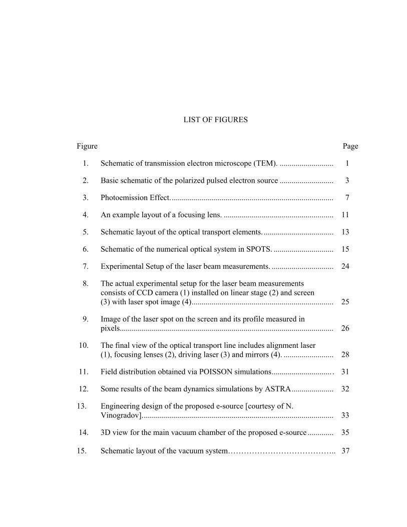
LIST OF FIGURES
Figure Page
1. Schematic of transmission electron microscope (TEM). ........................... 1
2. Basic schematic of the polarized pulsed electron source ........................... 3
3. Photoemission Effect.................................................................................. 7
4. An example layout of a focusing lens. ....................................................... 11
5. Schematic layout of the optical transport elements. ................................... 13
6. Schematic of the numerical optical system in SPOTS. .............................. 15
7. Experimental Setup of the laser beam measurements. ............................... 24
8. The actual experimental setup for the laser beam measurements consists of CCD camera (1) installed on linear stage (2) and screen (3) with laser spot image (4)....................................................................... 25
9. Image of the laser spot on the screen and its profile measured in pixels........................................................................................................... 26
10. The final view of the optical transport line includes alignment laser (1), focusing lenses (2), driving laser (3) and mirrors (4). ......................... 28
11. Field distribution obtained via POISSON simulations.............................. . 31
12. Some results of the beam dynamics simulations by ASTRA..................... 32
13. Engineering design of the proposed e-source [courtesy of N. Vinogradov]................................................................................................ 33
14. 3D view for the main vacuum chamber of the proposed e-source ............. 35 15. Schematic layout of the vacuum system………………………………….. 37

ix
Figure Page
16. Electron beam RMS size evolution in the source....................................... 41
17. Principle of the blade-scan technique......................................................... 42
18. Main Program’s Front panel....................................................................... 46
19. Front Panel of Main Program. .................................................................... 53
20. Motor init 3_1 Front Panel. ........................................................................ 54
21. Motor init 3_1 part Block Diagram. ........................................................... 55

LIST OF GRAPHS
Graph Page
1. Charge Estimation for quantum efficiency of 10-4 (light blue circle) and 10-5 (dark blue diamond) of copper.................................................. 9
2. Ray tracing Graph generated with SPOTS. ............................................. 16
3. Laser beam RMS envelope along the optical transport line .................... 18
4. The camera calibration for different distances between the camera and image on the measuring screen. [Courtesy of N. Vinogradov]................ 27
5. Pumpdown curve for vacuum Chamber. [Data courtesy of Leybold [9]]............................................................................................................ 38
6. An example of measurements with the blade (a) and the obtained beam profile (b)........................................................................................ 43

CHAPTER 1
INTRODUCTION
Standard microscopes use light as a source; hence the image is limited by the
wavelength of light. In an electron microscope the light is replaced by much lower
wavelength electrons, making it possible to attain much better resolution of a few
orders of angstroms (10-10 m). Current electron microscope sources provide a low
energy (10-100 keV) “pencil” electron beam. The beam is tightly focused on a to-be-
analyzed sample and the distribution of the transmitted electron is analyzed. This is
the basic concept of transmission electron microscopy (TEM). The electron beam is
generated via thermoionic emission from a hot cathode, and the beam is focused by
means of magnetic solenoidal lenses. See Figure 1.
Figure 1 - Schematic of transmission electron microscope (TEM).

2
Conventional electron microscopes have limitations; although they can provide
electron beam with sub-microns beam sizes, the electrons beam is not spin-polarized.
Spin-polarization of the electron beam would be an important step for probing some
magnetic phenomena. To enhance electron microscopy capability a pulsed electron
source capable of producing short spin-polarized electron beam is proposed. This
would require a photoemission source. A first step toward this development is to build
a prototype of the pulsed photoemission electron source without spin-polarization.
The Department of Physics of Northern Illinois University (NIU) is collaborating with
Argonne National Laboratory (ANL) on the development of such an inexpensive low
energy electron source. A schematic rendition of the proposed source appears in
Figure 2. A pulsed ultraviolet (UV) laser impinges on a copper photocathode and a
bunched electron beam is extracted and accelerated to approximately 15-30 keV by a
DC electric field established between the photocathode and anode.

3
Figure 2 - Basic schematic of the polarized pulsed electron source. The total footprint of the system is about 1x2 m.
The proof-of-principle electron source aims at producing a pulsed electron
beams with the parameters shown in Table 1. Eventually the source will be upgraded
to provide a spin-polarized, pulsed electron beam. The photocathode will be replaced
by a gallium Arsenide (GaAs) photocathode, and the laser changed to a circularly
polarized, wavelength-tunable laser operating at 800 nm.
4
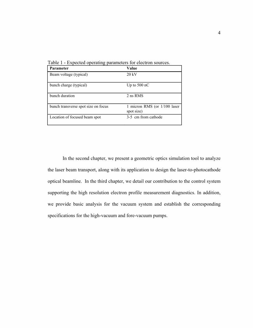
Table 1 - Expected operating parameters for electron sources. Parameter Value Beam voltage (typical) 20 kV
bunch charge (typical) Up to 500 nC
bunch duration 2 ns RMS
bunch transverse spot size on focus 1 micron RMS (or 1/100 laser spot size)
Location of focused beam spot 3-5 cm from cathode
In the second chapter, we present a geometric optics simulation tool to analyze
the laser beam transport, along with its application to design the laser-to-photocathode
optical beamline. In the third chapter, we detail our contribution to the control system
supporting the high resolution electron profile measurement diagnostics. In addition,
we provide basic analysis for the vacuum system and establish the corresponding
specifications for the high-vacuum and fore-vacuum pumps.
CHAPTER 2
THE PHOTOCATHODE DRIVE - LASER TRANSPORT
The purpose of this chapter is to detail the design and installation of an optical
transport line for the ultraviolet photocathode drive laser. In order to achieve these
goals we have estimated of the quantum efficiency for the copper cathode, done the
design and numerical studies of the optical transport line properties to establish the
lens location and focal strength, and made direct experimental measurements of the
laser beam properties for the designed optical transport. To address the first two
problems, a package of simulation codes called Simulated Path of Optical Transport
System (SPOTS) has been developed by using MathCAD 2001i.
2-1 – Photoemission
Photoemission, or the photoelectric effect, is a phenomenon in which
electrically charged particles are released from a material when it absorbs
electromagnetic radiation. In the present thesis, photoemission simply refers to the
ejection of electrons from a metal. This occurs only when the electrons in the metal
6
absorb a sufficient amount of energy from the light to escape from the metal. This
minimum energy is called the binding energy or work function W. The work function
is different for each type of metal. Energy absorbed in excess of this binding energy is
carried off by the electron as kinetic energy. Some of this kinetic energy may be
transferred to other electrons or atoms in the metal so that the electrons will have a
range of kinetic energies leaving the metal. Quantum theory states that the energy of
light is concentrated into discrete bundles called photons. For a given wavelength of
light, each photon has the same energy E = hf = hc/λ where h is a constant, f is the
frequency of the light, c is the speed of light, and λ its wavelength. The intensity of the
impinging light beam determines the rate of electron emission from the metal provided
that each photon has sufficient energy to eject an electron [1].
In the single-photon photoemission process, an electron absorbs the energy of
one photon and if it has more energy than the work function, then the electron is
ejected from the material. The excess energy hf – W appears as the electrons’ kinetic
energy; see Figure 3. A high vacuum is required to avoid interference of the light with
other matter such as residual gasses (see Chapter 3 for more information).

7
Figure 3 - Photoemission Effect.
A measure of photoemission yield is the quantum efficiency: the ratio of the
number of photoemitted electrons over the number of incident photons. Quantum
efficiencies of 1x10⁻⁵ for copper have been measured previously from a 266nm light
(hf=4.66 eV) which is slightly larger than the work function of Cu of (W=4.65 eV) [2].
The charge Q of the photoemitted electron bunch is given by
8
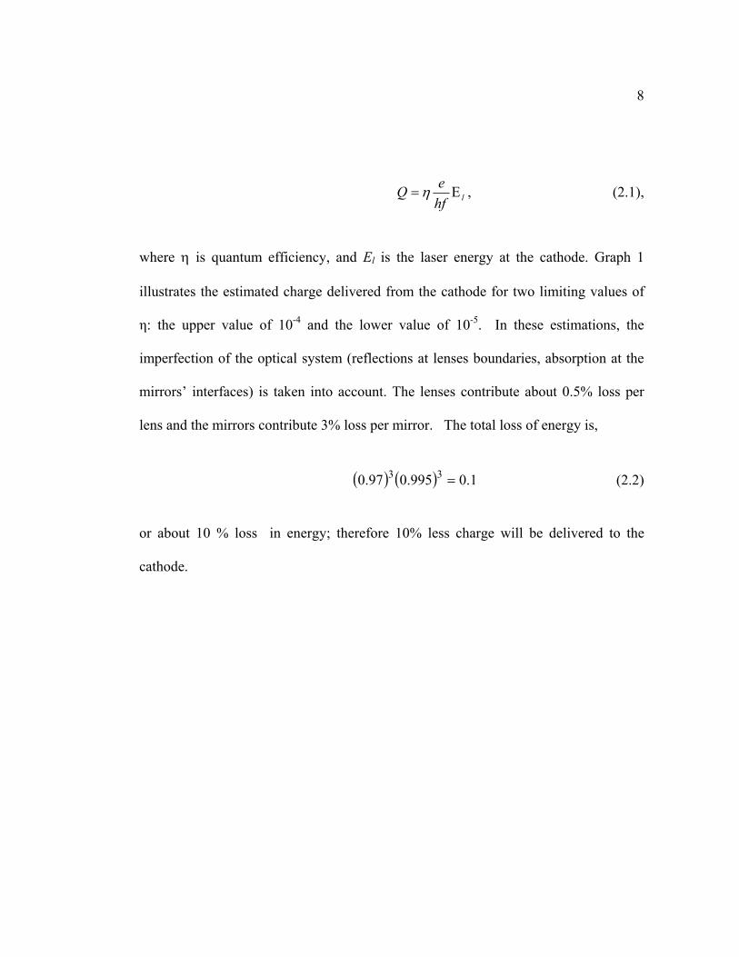
lhfeQ Ε=η , (2.1),
where η is quantum efficiency, and El is the laser energy at the cathode. Graph 1
illustrates the estimated charge delivered from the cathode for two limiting values of
η: the upper value of 10-4 and the lower value of 10-5. In these estimations, the
imperfection of the optical system (reflections at lenses boundaries, absorption at the
mirrors’ interfaces) is taken into account. The lenses contribute about 0.5% loss per
lens and the mirrors contribute 3% loss per mirror. The total loss of energy is,
( ) ( ) 1.0995.097.0 33 = (2.2)
or about 10 % loss in energy; therefore 10% less charge will be delivered to the
cathode.

9
Graph 1 – Charge Estimation for quantum efficiency of 10-4 (light blue circle) and 10-5 (dark blue diamond) of copper. The vertical line corresponds to the maximum energy that can be delivered by the laser at the photocathode.
The neodymium: yttrium-aluminum garnet (Nd:Yag) laser produces, after
frequency quadrupling, UV pulses (λ=266 nm) of 3 mJ. If we assume the quantum
efficiency of copper to be 10-5, the charge delivered to the cathode is 5.8 nC for the
maximum laser energy of 3 mJ. This lower limit case provides a charge much larger
than is needed for electron microscopy applications, which is around a few
picocoulombs.
10
2-2 – Laser Beam Transport Line
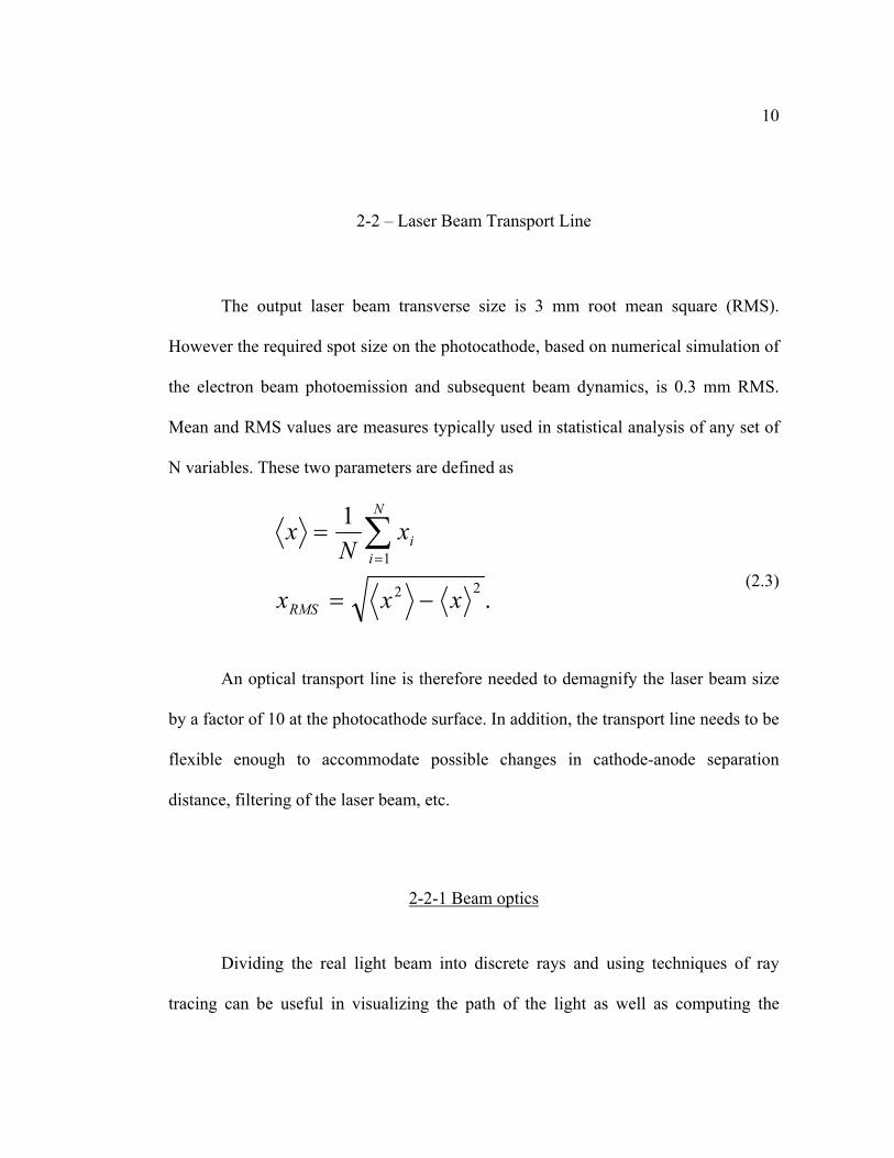
The output laser beam transverse size is 3 mm root mean square (RMS).
However the required spot size on the photocathode, based on numerical simulation of
the electron beam photoemission and subsequent beam dynamics, is 0.3 mm RMS.
Mean and RMS values are measures typically used in statistical analysis of any set of
N variables. These two parameters are defined as
.
1
22
1
xxx
xN
x
RMS
N
ii
−=
= ∑=
(2.3)
An optical transport line is therefore needed to demagnify the laser beam size
by a factor of 10 at the photocathode surface. In addition, the transport line needs to be
flexible enough to accommodate possible changes in cathode-anode separation
distance, filtering of the laser beam, etc.
2-2-1 Beam optics
Dividing the real light beam into discrete rays and using techniques of ray
tracing can be useful in visualizing the path of the light as well as computing the

11
propagation of light throughout the system. The technique of ray tracing is utilized to
find the characteristics of the beam envelope as it is propagating through the system.
This particular optical system contains the laser, three lenses, three mirrors, and a
cathode.
A lens is an object made with certain optical material that causes light to either
converge or diverge. In the present simulations the thin lens model, where the
thickness of the lens (d) is much less than the focal length (f), is used (see Figure 4).
The mirrors re-direct the beam in the optical system to fit the optical table.
Figure 4 - An example layout of a focusing lens.

12
Ray transfer matrix (or ABCD matrix) analysis is a type of ray tracing
technique used in optical systems. This technique is based on the paraxial
approximation which states that all rays are assumed to be at small angles and at small
distances from the optical axis. The matrix analysis depends on the optical system and
lens and drift matrices of the system must be ordered appropriately [3].
2-2-2 Numerical analysis of a three-lens optical system
The ultimate goal of the transport system is to deliver a 0.3 mm RMS beam at
the cathode surface. The transport system must also be tunable to accommodate
possible change of the cathode location. The photocathode drive laser beam is
transported to the copper cathode via three optical lenses and three mirrors as
illustrated in Figure 5 to fit the whole system on the optical table.

13
Figure 5 - Schematic layout of the optical transport elements.
The ray transfer matrix technique is utilized to perform the numerical study of
the optical system. The construction of the ray transfer matrix combines the drift
matrices
=
101 d
DM , (2.4)
as well as the thin lens matrices

14
−= 11
01
fLM .
(2.5) For the numerical study of this optical system the mirrors were neglected in the
calculations as they do not impact the beam properties. The matrix for the mirror is
the identity matrix
=
1001
MM , (2.6)
and hence does not change the light ray vector. Therefore, in the simulations, the
beam from the laser is transported through three thin lenses and focused before it
strikes the cathode, as depicted in the schematic in Figure 6.
In this system, the three thin lenses and the distances between them are
numerically depicted in Equation 2.7 for each light ray. The lenses’ focal lengths are
f1, f2 and f3 respectively, and the distances are d1-d4 respectively, as noted in Figure 6.

15
Figure 6 - Schematic of the numerical optical system in SPOTS.
The final position and divergence downstream of the system (x f, θ f) are
related to the initial value (x i, θ i) via a simple matrix multiplication:
−
−
−
=
i
i
f
f xd
f
d
f
d
f
dxθθ 10
11101
101
1101
101
1101
101 1
1
2
2
3
3
4 , (2.7)
where all the symbols are defined in Figure 6. The latter equation is used to ray trace
a large number of light rays. A statistical analysis can then be made and the moment
(average and RMS values) can be extracted. The MathCAD 2001i Software has been
implemented to perform these calculations (see section 2.3 of this chapter). Graph 2
depicts a number of light rays traveling the optical system.

16
Graph 2 - Ray tracing Graph generated with SPOTS. The lenses locations are schematically shown with the blue vertical lines.
2-3 – Simulation of optical system using MathCAD 2001i software
2-3-1 – What is MathCAD
MathCAD 2001i [4] is an integrating environment which combines standard
mathematical notations, text, and graphs in a single worksheet, making MathCAD
appropriate for knowledge capture, calculation reuse, and engineering collaboration.
MathCAD easily integrates with other applications, including Microsoft’s Excel.
17
2-3-2 – MathCAD Programming
Taking advantage of the matrix functionality, a beam envelope was developed
which included a system of three lenses and three mirrors within a package of codes
called Simulated Path of Optical Transport System (SPOTS). Both the lens matrix
(2.5) and the drift matrix (2.4) are employed in the SPOTS’ main function
characterizing the beam. The initial laser beam is numerically defined by a number of
points within set parameters. These parameters include beam RMS size, RMS
divergence, mean, and number of points (pts), which have a Gaussian distribution.
Thus a matrix of 1 x pts is created as the initial beam at the laser. Each column is a
random point in the beam with a random height (or RMS, radius) and a random drift.
Each row represents a particular point on the path of the lens system. As the light ray
travels, the ray changes direction, which is neatly presented in the matrix format. The
RMS of the collection of all the random beam particles at each point of interest in the
path from the laser to the cathode is also calculated and presented in Graph 3.

18
Graph 3 - Laser beam RMS envelope along the optical transport line. The lenses locations are schematically shown with the light blue arrows.
The divergence of each beam ray at each point of the pathway is also
calculated and accounted for in the second matrix. To numerically produce the
Gaussian beam, the RMS formula and average formula (2.3) are utilized.

19
2-3-3 - MathCAD Logic
SPOTS uses the following logic to develop the beam envelope from the laser,
the initial point, to the cathode or the terminating point: The lens matrix (Equation
2.5) and the drift matrix (Equation 2.4) are utilized in the program to calculate the
beam envelope as well as the path of individual points which make up the beam.
SPOTS allows the following parameters to be user-defined: These variable
parameters include the number of lenses (N), the number of random points (pts)
which made up the beam, the beam’s RMS size (rmsSize), and the RMS divergence
of the beam (rmsDiv) as well as the mean of the initial Gaussian beam. Other
variable parameters are the number of steps within each interval (nstep) where the
interval is the distance between each point of interest. The length matrix, L, is a 4X1
matrix of distances between points of interest, namely the laser and 1st lens, 1st lens
and 2nd lens, 2nd lens and 3rd lens, and 3rd lens and cathode. The focus matrix, F, is a
3x1 matrix of the focal lengths of the 3 lenses. Non-variable parameters use the
variable parameters and define the range of operations and are defined under the
heading of other parameters.
The random numbers generated to make up all the points initialized at the laser
use a MathCAD defined function, rnorm, which returns a column of numbers that
have a Gaussian or normalized distribution with a user-defined mean and variance.

20
Both the initial position and initial divergence of the rays that compose the beam are
distributed according to a Gaussian distribution. These two columns are then
reconfigured into a matrix of 2 x number of points to make the initial matrix of the
beam at the laser, which is labeled Matrix G. This initial matrix is then manipulated in
the R function, which takes advantage of the Lens and Drift matrices and outputs a
matrix, U, with (number of lens + 1) rows and (number of points) columns indicating
each particle’s position throughout the traveling path of the beam. The divergence of
each particle is also kept in the V matrix. The YY matrix is the entire position matrix
of each beam’s particle, including at the laser. XX is the one-column array of the path
location of the YY matrix.
SPOTS also displays the Gaussian distribution of the beam at the laser, at the
cathode, or right after each of the lenses. The user may select the location of the
beam, or the point of interest using the gaus parameter. Once gaus is defined, the
number of steps can also be selected; 100 is the default number of steps. Function h
utilizes the MathCAD defined function hist, which displays the histogram of the
row, hence the point of interest, of the matrix YY chosen. To get the Gaussian of the
distribution, the average and RMS of these points are calculated and utilized in the
Gaussian distribution graph. From here, the RMS envelope of the beam is a natural
development. Once this is graphed, RMS calculation at each point in the path needs to
be done. This calculation requires a separate function, function Cat, which is similar

21
to the R function in that it uses the lens and drift matrices. Cat requires an input of
the row of YY (or at the initial point of interest), the distance between the points of
interest as well as the focal length of the lens at the final point of interest. Cat
outputs a matrix of RMS calculated heights and divergences of the beam, with each
row representing a step in the path and each column once again representing each
particle of the beam. Each interval between the points of interest is calculated
separately and then combined in the graphing section to graph the RMS of the beam at
each step.
2-4 Experimental Studies of the Laser Beam Properties
The SPOTS program indicates that usage of a three-lens configuration is
optimal for the present application. The cathode is movable within the range of ±10
mm so this optimized configuration can be retuned to provide a focused spot of 0.3
mm on the cathode despite its changing location.
2-4-1 Description of laser and optical components

22
The photocathode drive laser is a Contimuum® MiniliteTM Nd: YAG laser
system. It is a pulsed high energy laser with the parameters listed in Table 2. It
incorporates a Nd:YAG rod producing a 50 mJ beam at 1064 nm. The beam is then
passed through two frequency doubling stages to finally yield a ~4 mJ, 266 nm laser
beam. The optical components used to build the transport line from the laser to the
cathode are listed in Table 3. The total length of this optical beamline is approximately
1 meter.
Table 2 - Minilite II Parameters. Description MiniliteII Energy (mJ) 4 Pulsewidth (nsec) 3-5 Linewidth (1/cm) 1 Divergence (mrad) < 3 Rod Diameter (mm) 3 Table 3 - Optical Devices Specifications. Item Manufacturer Comment Lens OFR 266 nm lens with a 300mm and
450 mm focusing length Mirror CVI Laser Contimuum® Nd:Yag, 266nm
2-4-2 Experimental setup for the laser beam measurements

23
The objective is to compare the numerically found RMS beam size to the
experimentally obtained RMS at a number of laser beam cross-sections. The
experimental setup places a mirror at the point of interest with a 45-degree tilt to the
optical axis, and a camera, also tilted at 45 degrees with respect to the mirror plane,
perpendicular to the laser beam axis. This setup, shown in Figure 7, incorporates a
COHU High Performance charge coupled device (CCD) camera installed on an MFA
series miniature linear motion stage supplied by Newport along with the ESP-300
Motion Controller operated from a remote PC via RS-232 port. The camera has a
640x480 pixel array and returns an image of the laser spot. Integrating this image
over the Y direction, one obtains the laser beam X-profile as the intensity (in relative
units) versus pixel number in the X direction (and vice versa) from which the laser
RMS size can be estimated. To find the correspondence between pixels and the actual
transverse distance within the beam (the pixel/mm ratio), the camera needs to be
calibrated. This can be done for any given setup by moving the camera across the
image at a known distance and measuring the shift of the image in pixels. The linear
stage allows the user to adjust the camera position with a high precision. After
calibration, the laser beam transverse intensity distribution can be renormalized as a
function of the transverse coordinate. The laser beam RMS envelope is obtained by
measuring the beam profile and calculating its RMS size at a number of points along
the optical path.

24
Figure 7 - Experimental Setup of the laser beam measurements.
2-4-3-Measurements
Figure 8 shows the actual experimental setup used for the laser beam
measurements. The typical laser spot image along with the laser beam profile is shown
in Figure 9. Calibration of the CCD camera has been done for different distances
between the mirror screen and the camera. According to the technique described in
the previous section, the results obtained appear in Graph 4. Each experimental point
is obtained by averaging the results of five independent measurements. Using this

25
calibration, the laser beam profile can be directly measured for any cross section of the
beam, thus allowing one to determine the actual envelope as a function of longitudinal
distance. The final configuration of the optical transport is demonstrated in Figure 10.
It includes the driving laser, alignment laser, three focusing lenses, and two mirrors.
The alignment laser produces visible light of very low power and is used to align the
optical system.
Figure 8 - The actual experimental setup for the laser beam measurements consists of CCD camera (1) installed on linear stage (2) and screen (3) with laser spot image (4).

26
Figure 9 - Image of the laser spot on the screen and its profile measured in pixels.

27
Graph 4 - The camera calibration for different distances between the camera and image on the measuring screen. [Courtesy of N. Vinogradov]

28
Figure 10 - The final view of the optical transport line includes the alignment laser (1), focusing lenses (2), driving laser (3) and mirrors (4).

CHAPTER 3
ELECTRON BEAM DIAGNOSTICS AND THE VACUUM SYSTEM
Any accelerator incorporates many diagnostic tools capable of measuring
various parameters, associated with the accelerated beam: longitudinal and transversal
bunch profile, total beam current, etc. One of the most important diagnostic tools is
the beam profiler, which is a device that allows the user to measure the transverse
and/or longitudinal intensity distribution within the beam.
The source being discussed has two types of diagnostics: a beam current
monitor and a transverse beam profiler. A conventional Faraday cup installed at the
end of the device is used to measure the total beam current: the electron beam is
dumped in a copper plate and the charge can be inferred. The profile detector
developed for this source has some remarkable features closely tied to the overall
design of the source itself and will be discussed in this chapter.
Contribution to the beam diagnostics for the proposed electron source consists
of development of a fully automated control system for profile measurements of the
beam. The system, created using the LabVIEW software [5], includes control of the
high precision linear actuators for beam scanning, data acquisition for the signal from

30
the measuring detectors, data analysis, etc. There are several difficulties related to the
beam diagnostic for this particular source such as the uncertainty of the exact location
of the focus, the ultra small beam size at the focus, and the very low energy of the
electron beam. The chapter describes how these difficulties have been overcome as
well as explains of the experimental setup along with the supporting software.
3-1 – The main principles of the source construction and operation
The computer simulation of the electrical field distribution in the source has been
performed earlier [6] using the SUPERFISH/POISSON code to optimize the cathode-
anode geometry in order to minimize the electron beam size at the location of its focus
(see Figure 11).

31
Cathode at high voltage
Anode (grounded)
Cathode at high voltage
Anode (grounded)
Figure 11 - Field distribution obtained via POISSON simulations. [The input file for this simulation was provided by J. Lewellen of Argonne National Lab).
The cathode is at 20 kV, while the anode is grounded. After the geometry of
the source electrodes had been established, the beam dynamics simulations were
performed using the ASTRA code [7, 8]. According to these simulations, done with
4•107 macroparticles, the electron beam with an initial RMS size of 0.3 mm has a
focus of less than 1 µm RMS located at a distance of about 39 mm from the cathode,
as illustrated in Figure 12.

32
Figure 12 - Some results of the beam dynamics simulations by ASTRA. Beam size evolution versus distance from the photocathode (bottom left), enlarged view around the focus location (upper right) and calculated transverse density (bottom right) [courtesy of N. Vinogradov].
Because of uncertainties in the numerical simulations, one needs to be capable
of measuring the transverse beam profile at a few points along the beam axis within a
certain longitudinal range. This latter capability of measuring the beam envelope
around the focus location is also important for the future development of the source.

33
One possible solution would consist of using a 2D stage, thereby providing the high
precision motion of the detector both the transversal and longitudinal directions. This
solution is, however, not effective: the design and operation of a 2D in-vacuum motion
actuator is costly and can cause some problems related to outgassing, which in turn
would spoil the vacuum and possibly deteriorate the cathode. This difficulty can be
overcome by using a specially designed vacuum chamber housing the source. The
engineering design of the proposed source appears in Figure 13 [6].
Figure 13 - Engineering design of the proposed e-source [courtesy of N. Vinogradov].

34
Cathode, anode, and anode holder form the actual source. The cathode holder
is connected to the vacuum feedthrough linear actuator (not shown) to adjust the
location of the cathode with respect to the anode if necessary. The cathode is mounted
on the holder using high voltage ceramic isolators rated up to 30 kV. The voltage is
applied to this electrode using the electrical feedthrough attached to the 2-3/4” CF
flange. The laser hits the cathode through the laser view port orientated at 45 degrees
with respect to the source axis. The detector corresponding to the horizontal transverse
profiler is inserted inside the vacuum chamber using high precision linear actuators
mounted on the 2-3/4” CF flange, called “measuring port” on the picture. A second
port (not shown) accommodates the vertical measurement. The whole backside flange
of the main chamber is installed on a heavy-duty manual linear stage (not shown). The
bellows are part of the vacuum chamber wall (see Figure 13) and accommodate
possible motion of the backside flange. Thus the cathode-anode assembly can be
moved longitudinally in the range of ± 10 mm. This allows beam envelope
measurements to be performed for different axial positions around the anticipated
location of the focus. A three-dimensional view of the main vacuum chamber is
shown in Figure 14.

35
Figure 14 - 3D view for the main vacuum chamber of the proposed e-source. 1 – Back side 6” CF flange to mount the anode holder and the linear actuator connected to the cathode holder; 2 – Two 2-3/4” CF flanges to mount the linear actuators for the transverse beam scan; 3 – One of two 1-1/3” CF flanges to install the low voltage feedthroughs for the signal pickup; 4 – 6” CF flange for the turbo pump; 5 – 2-3/4” CF flange to mount the high voltage feedthrough. 6 –2-3/4” CF flange to install the laser viewport; 7 - Front side 6” CF flange to mount a Faraday cup.

36
3-2 – Vacuum system design.
A high vacuum environment is required for successful operation of the source
to avoid interference of the electron beam with residual gases during the process of
photoemission and acceleration. The vacuum level of 10-7 Torr is expected to be
enough for commissioning of the source with a copper cathode. In order to achieve
this pressure, the complete vacuum system was modeled on a computer using
Leybold’s proprietary software, CompuVac [9]. The equipment considered for the
following calculations included a vacuum chamber, a fore pump and a turbomolecular
pump (TMP) as well as a hose connecting these two pumps (see Figure 15). The
chamber is made entirely of stainless steel and in this model is a cylinder of 15 inches
length and 4 inches diameter. The backing pump is Leybold’s SC 15 D scroll-pump
(pumping speed 35 l/s), and the TMP is Leybold’s Turbovac 151 Classicline (150 l/s),
connected to the SC 15 D through a flexible hose 4 feet long and 1 inch in diameter.

37
15 - Schematic layout of the vacuum system.
The initial pumping from atmospheric pressure down to about 10-2 Torr is
provided by the backing pump itself. Then the TMP can be started to pump the source
chamber down to the desired pressure of 10-7 Torr. The pumping time to reach this
pressure depends on the surface area of the vacuum chamber and the speed of the
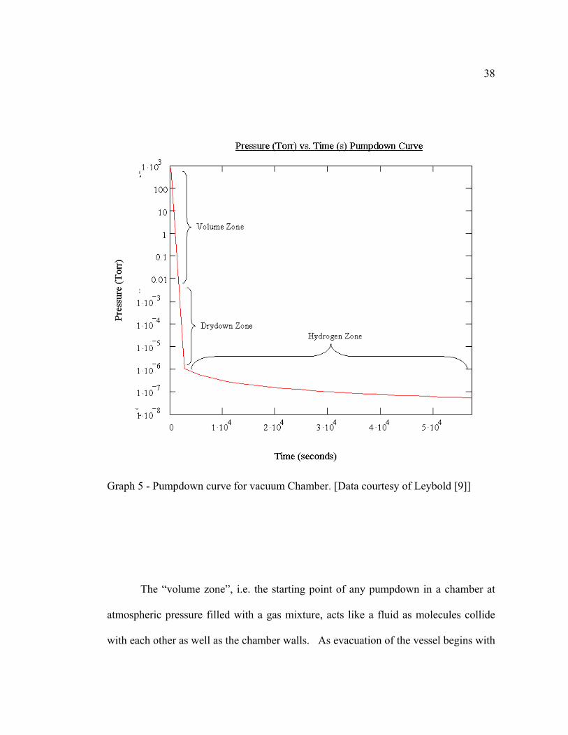
TMP [10]. As analyzed by Leybold [9], pumpdown time is 7½ hours to reach
1.06•10-7 Torr from 760 Torr. See Graph 5.
38
Graph 5 - Pumpdown curve for vacuum Chamber. [Data courtesy of Leybold [9]]
The “volume zone”, i.e. the starting point of any pumpdown in a chamber at
atmospheric pressure filled with a gas mixture, acts like a fluid as molecules collide
with each other as well as the chamber walls. As evacuation of the vessel begins with

39
the fore pump, the pressure will continue to fall as fewer and fewer molecules remain
in the chamber. When the chamber reaches a total pressure of between 10 and 20
Torr, the transitional gas flow region begins and water vapor starts to desorb from the
chamber's surfaces; however, it is only a small contribution to the overall pressure. As
the gases are pumped away, the desorbing water vapor begins to assume a higher
percentage of the total gas makeup as it steadily desorbs into the chamber's volume. At
the point, around 10-3 Torr, the “dry down zone” begins where the water vapor
becomes the predominant partial pressure. At this time, volume gases are diminished
and only a small portion of the desorbing molecules are pumped away. Although the
desorption rate will slowly fall as the bed of absorbed water molecules are pumped
away, a secondary water source then appears in the form of water vapor at the surfaces
and takes even more time to be pumped away, as they tend to absorb on the already
cleared surfaces. The “hydrogen zone” has pressure range called high and ultra-high
vacuum, less than 10-6 Torr, where most of the gas load, (H2) is from the material of
the chamber [11, 12].
The performed estimates show that the 150 l/s TMP in combination with the
35 l/s fore pump is capable of providing the required level of vacuum for the source.
Initial pumping of the source chamber from atmospheric pressure down to 10-7 Torr
will take about 7 hours. Once the vessel is pumped, this time is expected to be less for
a short-term maintenance venting of the chamber if the standard vacuum procedures

40
are followed: the vessel must be vented with dry nitrogen, and the surface of any new
part must be treated with alcohol prior to installation in the chamber.
3-3 – Beam profile measurements.
In the proposed electron source, the electron beam has an initial size of 0.3 mm
(RMS) at the photocathode. The beam is then focused to less than 1 micron
approximately 14 mm downstream of the anode as shown in Figure 16. Measuring
such a small electron beam size is a challenge. At the energies considered (15-30
keV), most of the standard diagnostic techniques, e.g. based on radiation, are not
applicable. Furthermore, the ultra small beam size anticipated at the focus also forbids
the use of standard techniques such as optical imaging of fluorescence induced by the
electron beam in a scintillating screen. The resolution of a conventional fluorescent
screen-type profile detector is limited by the grain size of the scintillating material,
which typically is a few microns or larger. Another method is based on wire-scanning:
a very thin wire scans across the beam and the charge intercepted by the wire is
recorded. This technique is limited in resolution by the size of the measuring wire,
whose diameter is usually no smaller than 1 micron.

41
Figure 16 - Electron beam RMS size evolution in the source. The 1 µm minimum spot size (39 mm from the photocathode) corresponds to the location of the beam profile diagnostics.
The blade-scanning technique is similar to the conventional wire-scan
detectors and has many similar advantages such as mechanical simplicity and
straightforward data acquisition. Unlike the conventional wire-scanners, resolution of
a blade scanner is not limited by wire thickness but by the quality of the blade edge.
The method consists of a blade, mounted on an electrically isolated holder, moving in
small steps across the beam (see Figure 17). The charge intercepted by the blade is
measured after each step. The typical result of such a scan is depicted in Graph 6a and
corresponds to a cumulative integral of the beam profile. Differentiation of this
measurement yields the beam profile as shown in Graph 6b. Therefore, if the quality

42
of the blade edge is high enough, resolution of the scan is defined by the size of each
step. Modern high precision linear actuators are capable of moving the measuring
blade with sub-micron resolution thus providing the accuracy needed to characterize
the focused beam in the proposed source.
Figure 17 - Principle of the blade-scan technique.

43
Graph 6 – An example of measurements with the blade (a) and the obtained beam profile (b).
3-3 – Programming Motion Controller using LabVIEW
3-3-1 - What is LabVIEW
The LabVIEW software package has been used to develop the control system
for the beam scan experiment. National Instruments LabVIEW 8.0 is an object-
oriented graphical programming language that includes all the standard features of a
general-purpose programming environment, such as data structures, looping
structures, and event handling. This software is specifically designed to provide
interface with measurement and control hardware. LabVIEW uses a programming
model that is highly intuitive for people familiar with block diagrams and flowcharts.

44
The flow of data between nodes determines the execution order in LabVIEW, so block
diagrams that execute multiple operations in parallel can be created. The debugging
tools, primarily a process known as execution highlighting, trace the data as it moves
through a program and show precisely how data passes from one node to another
along the wires.
With LabVIEW, graphical programming is combined with state of the art data
acquisition hardware and a PC. The motion controller, which operates the stepper
motor installed on the linear actuator, is connected to the PC through the serial port
(RS232). The code, made using LabVIEW, sends control commands via the serial port
to the device and receives information about motor status, current motor position, etc.
The combination of data acquisition, data analysis, and presentation of results has
made this particular code very useful in this project.
3-3-2 – LabVIEW Program
The main program (Figure 18) allows the user to turn on the motor as well as
control the motor’s movement. To run the program, the user needs to click on
Operate, and then on Run. The user may specify the port number and the axis
number of the motor connection with the computer. The program will initialize the
motor and find the range of its motion from 0 to a maximum limit, which is displayed

45
as MAX on the program. Once that has been established, the user may input a point at
which to start the stepping control motor and another to stop the motor. The user may
specify the number of steps to take between the two endpoints as well as the time
delay between each step. When the program is ready to move the motor, a green light
(Ready) will light up and clicking the MOVE button will start the motion. The user
may repeatedly redefine the parameters and move the motor until ready to exit the
program, when the STOP button may be pressed. If the program encounters any
problems while running, the error code will have a non-zero number and the
explanation of the nature of the error will be displayed in the comment box.

46
Figure 18 - Main Program’s Front panel.

47
3-3-3 – LabVIEW Programming Logic
The user is sees the front panel (Figure 18) and has access to the block
diagram. The main block diagram, ESP_MC_3_8.vi Block Diagram, is composed of
4 major steps or frames. The first frame initializes the motor by assigning parameters
specific to that motor. The motor is connected to motor port 2 and axis 1 as
default but the user may change these settings if desired. SubVI Motor_init_3_1.vi is
utilized to initialize the motor with its specifications. Once the motor is initialized
without errors, the program continues. Failsafe is installed in this program in the form
of error conditions every step of the way. After each step, the program confirms no
errors to continue. If an error is encountered the program displays it and
subsequent errors in the error out section and allows the user to correct it.
After successful initialization, the second frame is activated to find the range of
the motor using FindLimit.vi. Here one end is labeled 0 and the other end becomes
the maximum value. This maximum value is saved into a global variable, Max, to be
utilized later in the program as well as to let the user know the full range of the motor.
This step displays dialogue when moving to each extreme end of the stepping motor.
It ends with a displayed location of the stepping motor in the current motor
position. This range is in units defined in the program and is dependent on the
motor. For this application, each unit distance is smaller than a centimeter and varies
with each run of the program due to motor design.

48
Once the program has successfully established the range of the stepping motor,
the core of the program is galvanized in the third frame. At this time, the user is
allowed to input parameters on the front panel (shown in Figure 18) and press the
MOVE button, which activates the stepping motor. These parameters include Start,
End, StepNum, and Time between Steps. Start is the starting position of
the motor, and End is the ending position. Within this distance, the motor will take
StepNum number of steps and wait Time between Steps number of seconds
after each step. The current motor position will display the location of the
motor at each step. The green light illuminates when the motor has stopped moving,
indicating readiness of the motor to take more commands from the user. The program
allows the user to move the motor as many times as needed. This is achieved through
a “while” loop in the second frame, which continues until the user presses the STOP
button. If any errors occur during this stage the user is notified via the Motor
error out box on the Front Panel and is allowed to correct this error.
Motor error out keeps track of all errors occurring in the program. This
allows tracking of problems encountered during the current run of the program. This
is done in the “while” loop, where the program checks for errors at each step and the
following logic is applied. Once the MOVE button is activated, the program checks to
ensure that the starting position and ending position are within range and that the
ending position occurs after the starting position. If either or both of these conditions

49
are not met the motor is moved to the highest position of the entered parameter. If the
above parameters are satisfactory then the program checks to ensure that both the time
between steps and the number of steps are not less than zero. If either is less than or
equal to zero, the user is notified that these parameters are thusly defined and will be
regarded as zero in the program. Once these values are within acceptable limits, the
program moves forward as specified. At the end of the move, the program checks for
errors and continues if none are detected. The green light illuminates and the user
may move the motor again. This cycle continues until the user is finished and presses
the STOP button.
Once the user has pressed the STOP button on the main window, the fourth
frame is activated. This frame turns off the motor, and resets the parameters to the
default values. For a complete and detailed list of each of these programs and their
subVIs, see Appendix A.

CHAPTER 4
CONCLUSION
This thesis describes the efforts to develop a new photoemission-based
electron source. First a software package, Simulated Path of Optical Transport System
(SPOTS), has been written for numerical analysis of the photocathode drive laser
beam propagation in a user-defined optical system. The optical transport line to deliver
the laser beam from the laser to the source cathode has been simulated and designed
using the latter program. Based on the established specification for the laser beam
transport system, the optical components like lenses and mirrors have been purchased
and installed to provide the required properties of the laser spot on the cathode surface.
We performed initial measurements of the laser beam. Given the laser energy, the
electron bunch charge delivered by the copper cathode has been estimated and is well
over the required charge for electron microscopy. Since the source needs to be housed
in a vacuum chamber, analysis of the vacuum system has also been performed to
calculate the vacuum level. Finally, another program aimed at controlling one of the
electron beam diagnostics, the beam profile, has been developed. This software,
implemented using LabVIEW, is an integrated control system that provides the user
with automatic equipment control and data acquisition capabilities to be used in the
forthcoming commissioning of this electron source.

51
REFERENCES
[1] E. R. Hecht . Optics (2nd ed,), Adison-Wesley, (1987).
[2] Davis, P. Hairapetian, G. Clayton, C. et al. Quantum Efficiency Measurement of
a Copper Photocathode in an RF Electron Gun. IEEE PAC (1993). Retrieved
March 2007 from:
http://pbpl.physics.ucla.edu/Literature/_library/davis_1993_0252.pdf
[3] R.A. Serway. Physics for Scientists and Engineers (4th ed,), Philadelphia:
Harcourt Brace & Company (1997).
[4] Mathcad 2001i User’s Guide With Reference Manual. (2001). Cambridge, MA:
MathSoft Engineering & Education, Inc. http://www.mathsoft.com.
[5] LabVIEW 8.0. http://www.ni.com.
[6] N. Vinogradov, private communications.
[7] Flottmann, K, Lidia, S.M, Piot, P. Recent Improvements to the Astra Particle
Tracking Code. PAC 2003. http://www.desy.de/~mpyflo (2003).
[8] P.Piot, N. Vinogradov, private communications.
[9] A. Berry. Sales Support Engineer of Leybold, private communications. 2007
[10] Lafferty, J.M. (Eds). Foundations of Vacuum Science and Technology. New
York: John Wiley & Sons, Inc (1998).
[11] P.Danielson. A Journal of Practical and Useful Vacuum Technology. Retrieved
January, 2007 from http://www.vacuumlab.com. (2004).
[12] P. Danielson (2007) Private communicatons.

52
APPENDIX A
SUB VI DOCUMENTATION The following Sub VIs used LabVIEW 8: The main program that allows you to view the control and run the necessary application is 0under Shafaq/Work/Motion/ESP_MC_3_8. This program uses an hierarchy system to implement the stepping motor motion control. Notes: def = default. User button, input parameter, output parameter
Motor Error Out = Error Out is the output in most sub vis that become the input (Error In) in the next step of the code. If there is an error, the error is carried all the way to the last step and description is available to the user for help in input parameters).
SUB VI: ESP_MC_3_8.vi: Input(s):
Motor Port # (def = 2): the port the motor is plugged into. Axis # (def = 1): the axis the motor is defined as. Start (def = 0): the starting position for the stepping motor. End (def = 0): the ending position for the stepping motor. StepNum (def = 1): The number of steps the motor has to take between start and end Time between Steps (sec): The amount of time delay between each step in seconds.
Description: At the beginning of each run, the motor automatically moves to one extrema and then to the other extrema and displays the maximum moving distance of the motor (MAX). Current Motor Position is always displayed. The user must press MOVE Button to start moving the motor during steps. Error message with comment is given if one or more of the parameters is not in accordance with other parameters. The program may be stopped at any time by pressing the STOP button. The Ready button is lit when the motor is ready to be moved. Figure 19 displays the user-friendly front panel of this program. Output(s): Moved Motor, Maximum distance of motor, current motor position and Motor Error Out. Sub Vi utilized:
i. Motor init 3_1.vi ii. Find Limit.vi

53
iii. Motor write.vi iv. Current Position.vi v. Motor step 2.vi
vi. Motor write.vi vii. User display messages to User 3, User 4, and User 5
Figure 19 - Front Panel of Main Program.

54
Motor init_3_1.vi: Input(s):
Error in (def = 0): the error code from previous steps of the whole code Motor Port # (def = 2): the port the motor is plugged into. Axis # (def = 1): the axis the motor is defined as.
Description: Initializes the motor. Checks to see if motor is connected and everything is set to go. If no errors, moves the motor to initial position and displays current position. Figure 20 displays the motor initialization part of the main program while Figure 21 displays the inner block diagram or programming of this motor initialization. Output(s): Motor Error Out. Sub Vi utilized:
i. Motor read.vi ii. HardwareStatus1.vi
iii. Motor write.vi iv. Serial Port Init.vi (pre-defined in Labview 8.0)
Figure 20 - Motor init 3_1 Front Panel.

55
Figure 21 - Motor init 3_1 part Block Diagram.

56
MaxFa - global variable. Input(s):
MaxMFA(def=26): Maximum moving distance of stepping motor.
Description: Saves the maximum moving distance of the stepping motor from the initial run of the ESP_MC_3_8.vi. Output(s): MaxMFA. Motor step 2.vi: Input(s):
Error in (def = 0): the error code from previous steps of the whole code. Port # (def = 0): the port the motor is plugged in Axis # (def = 1): the axis the motor is defined as. SM steps (def = 0): The number of steps the motor has to take. Waitsize (def = 1): The amount of time delay between each step in seconds: this program adds ½ second to it.
Description: This program utilizes another subvi ( Motor move.vi) to move the motor with the above parameters. Output(s): Moved Motor, Motor Error Out. Sub Vi utilized: Motor move.vi Find Limit.vi: Input(s):
Error in (def = 0): the error code from previous steps of the whole code Motor Port # (def = 2): the port the motor is plugged into. Axis # (def = 1): the axis the motor is defined as. POS OR NEG: The direction of the motor extrema. Wait (def = 1): The amount of time delay after move command in seconds: this program adds ½ second to it.
Description: Finds the extreme limit of the stepping motor’s traveling distance in either positive or negative direction. Output(s): Position Status, Motor Error Out. Sub Vi utilized:
i. Motor read.vi ii. Current Position.vi
iii. Motor write.vi

57
MaxFa - global variable. Input(s):
MaxMFA(def=26): Maximum moving distance of stepping motor.
Description: Saves the maximum moving distance of the stepping motor from the initial run of the ESP_MC_3_8.vi. Output(s): MaxMFA. Motor move.vi: Input(s):
Error in (def = 0): the error code from previous steps of the whole code Motor Port # (def = 2): the port the motor is plugged into. Axis # (def = 1): the axis the motor is defined as. Pos. SM (def = 0): the position user wants to move to.
Description: Moves the motor to the position defined in Pos SM in one step. Output(s): Motor Error Out. Sub Vi utilized: Motor write.vi Current Position.vi: Input(s):
Error in (def = 0): the error code from previous steps of the whole code Motor Port # (def = 2): the port the motor is plugged into. Axis # (def = 1): the axis the motor is defined as.
Terminator (def = ): ends the command to the motor. Description: Finds the current position of the motor in relation to the one extrema of the stepping motor being 0 and the other being MaxMFA. Output(s): Position Status, Motor Error Out. Sub Vi utilized:
i. Bytes At Serial Port.vi (pre-defined in LabView 8.0). ii. Serial Port Read.vi (pre-defined in LabView 8.0).
iii. Serial Port Write.vi (pre-defined in LabView 8.0). HardwareStatus1.vi: Input(s):

58
Motor Port # (def = 2): the port the motor is plugged into. Axis # (def = 1): the axis the motor is defined as.
Description: Finds which axis is connected to the port and reports to motor answer. If no axis is connected, return that answer. Utilizes substring before match and after substring to determine axis connection. The status light is lit if there is an axis connection. Output(s): Motor answer. Sub Vi utilized:
i. Motor read.vi ii. Motor write.vi
Motor read.vi: Input(s):
Motor Port # (def = 2): the port the motor is plugged into. Axis # (def = 1): the axis the motor is defined as.
Description: Reads in answers/commands from the program to the software. Output(s): Motor answer, Motor Error Out. Sub Vi utilized:
i. Bytes at Serial Port.vi (pre-defined in Labview 8.0). ii. Serial Port Read.vi (pre-defined in Labview 8.0).
Motor write.vi Input(s):
Motor Port # (def = 2): the port the motor is plugged into. Axis # (def = 1): the axis the motor is defined as.
Terminator (def = ): ends the command to the motor Command (def = ): the 2 letter command code to the port (or motor) Description: Sends the command from the user (of software) to the motor. Output(s): Error Out. Sub Vi utilized: Serial Port Write.vi (pre-defined in Labview 8.0). Ex_CorrectErrorChain.vi: (pre-defined in Labview 8.0??) Input(s):
Error In Description: Read in error code, displays Error Out code.

59
Output(s): Error Out. Few Sub Vi NOT USED in ESP_MC_3_8.vi but still can be used are: AxisDetermination.vi: Input(s):
Motor Port # (def = 2): the port the motor is plugged into. Axis # (def = 1): the axis the motor is defined as.
Description: Determines which axis is connected and displays this message in response, axis # and Motor answer as well as tells the 4-digit hex command which led to this determination in after substring. This is to ensure or check which axis is connected. Output(s): Motor answer. Response, axis # and after substring.. Command and Return.vi: Input(s):
Motor Port # (def = 2): the port the motor is plugged into. Axis # (def = 1): the axis the motor is defined as. Command (def = LP): the command sent to the motor from the user
Description: Gives commands to the motor, and sends it back to the user. This is to check to see if the commands are working. Output(s): Motor answer. Move steps.vi: Input(s):
Motor Port # (def = 2): the port the motor is plugged into. Axis # (def = 1): the axis the motor is defined as.
Target motor position (def=0): where the motor needs to be moved Steps (def = 1): The number of steps the motor needs to take to reach target motor position.
Description: Moves the motor to the target position in the number of steps with slight time delay between each step to accommodate the time it takes for the motor to move that prescribed distance. Output(s): Total Distance – motor has to travel. Step Size –

60
Current motor position – at each step including starting and ending. PS in Loop – position in loop.
Sub Vi utilized:
i. Current Position.vi ii. Motor step 2.vi
Motor step 2.vi: Input(s):
Error In (def = 0): error code in. Motor Port # (def = 2): the port the motor is plugged into. Axis # (def = 1): the axis the motor is defined as. SM steps (def = 0): The number of steps the motor has to take. Waitsize (def = 1): The amount of time delay between each step in seconds: this program adds ½ second to it.
Description: Moves the motor in number of steps. Has a time delay of Waitsize after each step. Output(s): Error Out. Sub Vi utilized: Motor move.vi (described above) Motor Position.vi: Input(s):
Motor Port # (def = 2): the port the motor is plugged into. Axis # (def = 1): the axis the motor is defined as. SM steps (def = 0): The number of steps the motor has to take.
Description: Sends command to motor to give the position of the motor. Output(s): Error Out, Answer. Sub Vi utilized:
i. Motor read.vi ii. Motor write.vi
Motor init 3.vi: Input(s):
Error In (def = 0): error code in. Motor Port # (def = 2): the port the motor is plugged into. Axis # (def = 1): the axis the motor is defined as.

61
Description: Simply initializes the motor. Output(s): Error Out. Sub Vi utilized:
i. Motor read.vi ii. Motor write.vi
iii. Serial Port Init.vi (pre-defined in Labview 8.0)
Find Range.vi: Input(s):
Error In (def = 0): error code in. Motor Port # (def = 2): the port the motor is plugged into. Axis # (def = 1): the axis the motor is defined as.
Description: Initializes motor. Finds the range of the motor. Sets one extrema at 0 and finds the Max value of the other extrema. Output(s): Error Out. Max Value, MaxMFA, Current Position Sub Vi utilized:
1. MotorInit_3_1, 2. CurrentPosition.vi 3. MaxMFA (global variable) 4. MotorWrite.vi
RangeSet.vi: Input(s):
Error In (def = 0): error code in. Motor Port # (def = 2): the port the motor is plugged into. Axis # (def = 1): the axis the motor is defined as. Current Position: Position of motion control motor.
Description: Initializes motor. Uses Find Range.vi to set extremas. Output(s): Error Out. Max value. MaxFa, Current Position. Sub Vi utilized:
1. MotorInit_3_1, 2. Find Range.vi, 3. MaxMFA (global variable) 4. MotorWrite.vi