Embed Size (px)
Citation preview

arX
iv:m
ath/
0105
082v
2 [
mat
h.D
S] 3
Oct
200
2
MORSE THEORY ON SPACES OF BRAIDS AND LAGRANGIAN DYNAMICS
R.W. GHRIST, J.B. VAN DEN BERG, AND R.C. VANDERVORST
ABSTRACT. In the first half of the paper we construct a Morse-type theory on certainspaces of braid diagrams. We define a topological invariant of closed positive braidswhich is correlated with the existence of invariant sets of parabolic flows defined on dis-cretized braid spaces. Parabolic flows, a type of one-dimensional lattice dynamics, evolvesingular braid diagrams in such a way as to decrease their topological complexity; alge-braic lengths decrease monotonically. This topological invariant is derived from a Morse-Conley homotopy index.
In the second half of the paper we apply this technology to second order Lagrangiansvia a discrete formulation of the variational problem. This culminates in a very generalforcing theorem for the existence of infinitely many braid classes of closed orbits.
1. PRELUDE
It is well-known that under the evolution of any scalar uniformly parabolic equationof the form
(1) ut = f(x, u, ux, uxx) ; ∂uxxf ≥ δ > 0,
the graphs of two solutions u1(x, t) and u2(x, t) evolve in such a way that the number ofintersections of the graphs does not increase in time. This principle, known in variouscircles as “comparison principle” or “lap number” techniques, entwines the geometryof the graphs (uxx is a curvature term), the topology of the solutions (the intersectionnumber is a local linking number), and the local dynamics of the PDE. This is a valu-able approach for understanding local dynamics for a wide variety of flows exhibitingparabolic behavior with both classical [54] and contemporary [41, 5, 10, 19] implications.
This paper is an extension of this local technique to a global technique. One suchwell-established globalization appears in the work of Angenent on curve-shortening [4]:evolving closed curves on a surface by curve shortening isolates the classes of curvesdynamically and implies a monotonicity with respect to number of self-intersections.
In contrast, one could consider the following topological globalization. Superimpos-ing the graphs of a collection of functions uα(x) gives something which resembles theprojection of a topological braid onto the plane. Assume that the “height” of the strandsabove the page is given by the slope uαx(x), or, equivalently, that all of the crossingsin the projection are of the same sign (bottom-over-top): see Fig. 1[left]. Evolving thesefunctions under a parabolic equation (with, say, boundary endpoints fixed) yields a flowon a certain space of braid diagrams which has a topological monotonicity: linking can bedestroyed but not created. This establishes a partial ordering on the semigroup of positive
Date: October 25, 2018.The first author was supported by NSF DMS-9971629 and NSF DMS-0134408. The second author was
supported by an EPSRC Fellowship. The third author was supported by NWO Vidi-grant 639.032.202.
1

2 R.W. GHRIST, J.B. VAN DEN BERG, AND R.C. VANDERVORST
braids which is respected by parabolic dynamics. The idea of topological braid classeswith this partial ordering is a globalization of the lap number (which, in braid-theoreticterms becomes the length of the braid in the braid group under standard generators).
1.1. Parabolic flows on spaces of braid diagrams. In this paper, we initiate the studyof parabolic flows on spaces of braid diagrams. The particular braids in question will
be (a) positive – all crossings are considered to be of the same sign; (b) closed1 – the leftand right sides are identified; and (c) discretized – or piecewise linear with fixed distancebetween “anchor points,” so as to avoid the analytic difficulties of working on infinitedimensional spaces of curves. See Fig. 1 for examples of braid diagrams.
PSfrag replacements
xx x
uu u
ux
FIGURE 1. Curves in the x− u plane [left] lift to a braid [center] whichis then discretized [right]. In a discretized isotopy, one slides the anchorpoints vertically.
The flows we consider evolve the anchor points of the braid diagram so that the braidclass can change, but only so as to decrease complexity: local linking of strands may notincrease with time. Due to the close similarity with parabolic partial differential equa-tions such systems will be referred to as parabolic recurrence relations, and the inducedflows as parabolic flows. These flows are given by
d
dtui = Ri(ui−1, ui, ui+1),(2)
where the variables ui represent the vertical positions of the ordered anchor points ofdiscrete braid diagrams. The only conditions imposed on the dynamics is the mono-tonicity condition that every Ri be increasing functions of ui−1 and ui+1.
While a discretization of a PDE of the form (1) with nearest-neighbor interactionyields a parabolic recurrence relation, the class of dynamics we consider is significantlylarger in scope (see, e.g., [40]). Parabolic recurrence relations are a sub-class of monotonerecurrence relations as studied in [3] and [26].
The evolution of braid diagrams yields a situation not unlike that considered by Vas-siliev in knot theory [59]: in our scenario, the space of all braid diagrams is partitionedby the discriminant of singular diagrams into the braid classes. The parabolic flowswe consider are transverse to these singular varieties (except for a set of “collapsed”braids) and are co-oriented in a direction along which the algebraic length of the braiddecreases: this is an algebraic version of curve shortening.
To proceed, two types of noncompactness on spaces of braid diagrams must be re-paired. Most severe is the problem of braid strands completely collapsing onto one
1The theory works equally well for braids with fixed endpoints.

MORSE THEORY ON SPACES OF BRAIDS 3
another. To resolve this type of noncompactness, we assume that the dynamics fixessome collection of braid strands, a skeleton, and then work on spaces of braid pairs:one free, one fixed. The relative theory then leads to forcing results of the type “Givena stationary braid class, which other braids are forced as invariant sets of parabolicflows?” The second type of noncompactness in the dynamics occurs when the braidstrands are free to evolve to arbitrarily large values. In the PDE setting, one requiresknowledge of boundary conditions at infinity to prove theorems about the dynamics. Inour braid-theoretic context, we convert boundary conditions to “artificial” braid strandsaugmented to the fixed skeleton.
Thus, working on spaces of braid pairs, the dynamics at the discriminant permits theconstruction of a Morse theory in the spirit of Conley to detect invariant sets of para-bolic flows. Conley’s extension of the Morse index associates to any sufficiently isolatedinvariant set a space whose homotopy type measures not merely the dimension of theunstable manifold (the Morse index) but rather the coarse topological features of the un-stable dynamics associated to this set. We obtain a well-defined Conley index for braiddiagrams from the monotonicity properties of parabolic flows. To be more precise, rela-tive braid classes (equivalence classes of isotopic braid diagrams fixing some skeleton)serve as candidates for isolating neighborhoods to which the Conley index can be as-signed. This approach is reminiscent of the ideas of linking of periodic orbits used byAngenent [2, 4] and LeCalvez [36, 37].
Our finite-dimensional approximations to the (infinite-dimensional) space of smoothtopological braids conceivably alter the Morse-theoretic properties of the discretizedbraid classes. One would like to know that so long as the discretization is not degen-erately coarse, the homotopy index is independent of both the discretization and thespecific parabolic flow employed. This is true. The principal topological result of thiswork is that the homotopy index is indeed an invariant of the topological (relative)braid class: see Theorems 19 and 20 for details. These theorems seem to evade a simplealgebraic-topological proof. The proof we employ in §5 constructs the appropriate ho-motopy by recasting the problem into singular dynamics and applying techniques fromsingular perturbation theory.
We thus obtain a topological index which can, like the Morse index, force the ex-istence of invariant sets. Specifically, a non-vanishing homotopy index for a relativebraid class indicates that there is an invariant set in this braid class for any parabolicflow with the appropriate skeleton. This is the foundation for the applications to followin the remainder of the paper.
The remainder of the paper explores applications of the machinery to a broad classof Lagrangian dynamics.
1.2. Second order Lagrangian dynamics. Our principal application of the Morse the-ory on discretized braids is to the problem of finding periodic orbits of second orderLagrangian systems: that is, Lagrangians of the form L(u, ux, uxx) where L ∈ C2(R3).An important motivation for studying such systems comes from the stationary Swift-Hohenberg model in physics, which is described by the fourth order equation
(1 +
d2
dx2
)2
u− αu + u3 = 0, α ∈ R.(3)

4 R.W. GHRIST, J.B. VAN DEN BERG, AND R.C. VANDERVORST
This equation is the Euler-Lagrange equation of the second order Lagrangian
(4) L(u, ux, uxx) =1
2|uxx|2 − |ux|2 +
1− α
2u2 +
1
4u4.
We generalize to the broadest possible class of second order Lagrangians. One beginswith the conventional convexity assumption, ∂2wL(u, v, w) ≥ δ > 0. The objective isto find bounded functions u : R → R which are stationary for the action integralJ [u] :=
∫L(u, ux, uxx)dx. Such functions u are bounded solutions of the Euler-Lagrange
equations
(5)d2
dx2∂L
∂uxx− d
dx
∂L
∂ux+∂L
∂u= 0.
Due to the translation invariance x 7→ x + c, the solutions of (5) satisfy the energyconstraint
(6)( ∂L∂ux
− d
dx
∂L
∂uxx
)ux +
∂L
∂uxxuxx − L(u, ux, uxx) = E = constant,
where E is the energy of a solution. To find bounded solutions for given values of E,
we employ the variational principle δu,T∫ T
0
(L(u, ux, uxx) + E
)dx = 0, which forces
solutions of (5) to have energy E. The Lagrangian problem can be reformulated as atwo degree-of-freedom Hamiltonian system; in that context, bounded periodic solutionsare closed characteristics of the (corresponding) energy manifold M3 ⊂ R4. Unlike thecase of first-order Lagrangian systems, the energy hypersurface is not of contact type ingeneral [6], and the recent stunning results in contact homology [16] are inapplicable.
The variational principle can be discretized for a certain considerable class of secondorder Lagrangians: those for which monotone laps between consecutive extrema uiare unique and continuous with respect to the endpoints. We give a precise definition in§8, denoting these as (second order Lagrangian) twist systems. Due to the energy iden-tity (6) the extrema ui are restricted to the set UE = u | L(u, 0, 0)+E ≥ 0, connectedcomponents of which are called interval components and denoted by IE . An energy levelis called regular if ∂L
∂u (u, 0, 0) 6= 0 for all u satisfying L(u, 0, 0) + E = 0. In order todeal with non-compact interval components IE certain asymptotic behavior has to bespecified, for example that “infinity” is attracting. Such Lagrangians are called dissipa-tive, and are most common in models coming from physics, like the Swift-HohenbergLagrangian. For a precise definition of dissipativity see §9. Other asymptotic behaviorsmay be considered as well, such as “infinity” is repelling, or more generally that infinityis isolating, implying that closed characteristics are a priori bounded in L∞.
Closed characteristics are either simple or non-simple depending on whether u(x), rep-resented as a closed curve in the (u, ux)-plane, is a simple closed curve or not. Thisdistinction is a sufficient language for the following general forcing theorem:
Theorem 1. Any dissipative twist system possessing a non-simple closed characteristic u(x) ata regular energy valueE such that u(x) ∈ IE , must possess an infinite number of (non-isotopic)closed characteristics at the same energy level as u(x).
This is the optimal type of forcing result: there are neither hidden assumptions aboutnondegeneracy of the orbits, nor restrictions to generic behavior. Sharpness comes fromthe fact that there exist systems with finitely many simple closed characteristics at eachenergy level.

MORSE THEORY ON SPACES OF BRAIDS 5
The above result raises the following question: when does an energy manifold con-tain a non-simple closed characteristic? In general the existence of such characteristicsdepends on the geometry of the energy manifold. One geometric property that sparksthe existence of non-simple closed characteristics is a singularity or near-singularity ofthe energy manifold. This, coupled with Theorem 1, triggers the existence of infinitelymany closed characteristics. The results that can be proved in this context (dissipa-tive twist systems) give a complete classification with respect to the existence of finitelymany versus infinitely many closed characteristics on singular energy levels. The firstresult in this direction deals with singular energy values for which IE = R.
Theorem 2. Suppose that a dissipative twist system has a singular energy levelE with IE = R,which contains two or more rest points. Then the system has infinitely many closed characteris-
tics at energy level E.2
Complementary to the above situation is the case when IE contains exactly one restpoint. To have infinitely many closed characteristics, the nature of the rest point willcome into play. If the rest point is a center (four imaginary eigenvalues), then the system hasinfinitely many closed characteristics at each energy level sufficiently close to E, including E. Ifthe rest point is not a center, there need not exist infinitely many closed characteristicsas results in [57] indicate.
Similar results can be proved for compact interval components (for which dissipativ-ity is irrelevant) and semi-infinite interval components IE ≃ R±.
Theorem 3. Suppose that a dissipative twist system has a singular energy level E with aninterval component IE = [a, b], or IE ≃ R±, which contains at least one rest point of saddle-focus/center type. Then the system has infinitely many closed characteristics at energy levelE.
If an interval component contains no rest points, or only degenerate rest points (0eigenvalues), then there need not exist infinitely many closed characteristics, complet-ing our classification.
This classification immediately applies to the Swift-Hohenberg model (3), which is atwist system for all parameter values α ∈ R. We leave it to the reader to apply the abovetheorems to the different regimes of α.
1.3. Additional applications. The framework of parabolic recurrence relations that weconstruct is robust enough to accommodate several other important classes of dynam-ics.
1.3.1. First-order nonautonomous Lagrangians. Finding periodic solutions of first-orderLagrangian systems of the form δ
∫L(x, u, ux)dx = 0, with L being 1-periodic in x, can
be rephrased in terms of parabolic recurrence relations of gradient type. The homotopyindex can be used to find periodic solutions u(x) in this setting, even though a globallydefined Poincare map on R2 need not exist.
2From the proof of this theorem in §9 it follows that the statement remains true for energy values E + c,
with c > 0 small.

6 R.W. GHRIST, J.B. VAN DEN BERG, AND R.C. VANDERVORST
1.3.2. Monotone twist maps. A monotone twist map (compare [3, 48]) is a (not necessarilyarea-preserving) map on R2 of the form
(u, pu) → (u′, p′u),∂u′
∂pu> 0.
Periodic orbits (ui, pui) are found by solving a parabolic recurrence relation for the
u-coordinates derived from the twist property.
1.3.3. Uniformly parabolic PDE’s. The study of the invariant dynamics of Equation (1)can also be formulated in terms of parabolic recurrence relations by a spatial discretiza-tion. The basic theory for braid forcing developed here can be adapted to the dynamicsof Equation (1): see [24] for details.
1.3.4. Lattice dynamics. The form of a parabolic recurrence relation is precisely that aris-ing from a set of coupled oscillators on a [periodic] one-dimensional lattice with nearest-neighbor attractive coupling. A similar setup arises in Aubry-LeDaeron-Mather theoryof the Frenkel-Kontorova model [7]. In this setting, a nontrivial homotopy index yieldsexistence of invariant states (or stationary, in the exact context) within a particular braidclass. Related physical systems (e.g., charge density waves on a 1-d lattice [45]) are alsooften reducible to parabolic recurrence relations.
1.4. History and outline. The history of our approach is the convergence of ideas fromknot theory, the dynamics of annulus twist maps, and curve shortening. We have al-ready mentioned the similarities with Vassiliev’s topological approach to discriminantsin the space of immersed knots. From the dynamical systems perspective, the studyof parabolic flows and gradient flows in relation with embedding data and the Con-ley index can be found in work of Angenent [2, 3, 4] and Le Calvez [36, 37] on areapreserving twist maps. More general studies of dynamical properties of parabolic-typeflows appear in numerous works: we have been inspired by the work of Smillie [53],Mallet-Paret and Smith [39], Hirsch [26], and, most strongly, the work of Angenent oncurve shortening [4]. Many of our applications to finding closed characteristics of sec-ond order Lagrangian systems share similar goals with the programme of Hofer andhis collaborators (see, e.g., [16, 27, 28]), with the novelty that our energy surfaces are allnon-compact and not necessarily of contact type [6].
Clearly there is a parallel between the homotopy index theory presented here andBoyland’s adaptation of Nielsen-Thurston theory for braid types of surface diffeomor-phisms [9]. An important difference is that we require compactness only at the level ofbraid diagrams, which does not yield compactness on the level of the domains of thereturn maps [if these indeed exist]. Another important observation is that the recur-rence relations are sometimes not defined on all of R2, which makes it very hard if notimpossible to rephrase the problem of finding periodic solutions in terms of fixed pointsof 2-dimensional maps.
There are three components of this paper: (a) the precise definitions of the spacesinvolved and flows constructed, covered in §2-§3; (b) the establishment of existence,invariance, and properties of the index for braid diagrams in §4-§7; and (c) applicationsof the machinery to second order Lagrangian systems §8-§10. Finally, §11 contains openquestions and remarks.

MORSE THEORY ON SPACES OF BRAIDS 7
Acknowledgments. The authors would like express special gratitude to Sigurd An-genent and Konstantin Mischaikow for numerous enlightening discussions. Specialthanks to Madjid Allili for his computational work in the earliest stages of this work.Finally, the hard work of the referee has improved the paper in several respects, espe-cially in the definitions of equivalent relative braid classes.
CONTENTS
1. Prelude 12. Spaces of discretized braid diagrams 73. Parabolic recurrence relations 104. The homotopy index for discretized braids 145. Stabilization and invariance 196. Duality 277. Morse theory 308. Second order Lagrangian systems 329. Multiplicity of closed characteristics 3710. Computation of the homotopy index 4611. Postlude 49References 52Appendix A. Construction of parabolic flows 54
2. SPACES OF DISCRETIZED BRAID DIAGRAMS
2.1. Definitions. Recall the definition of a braid (see [8, 25] for a comprehensive intro-duction). A braid β on n strands is a collection of embeddings βα : [0, 1] → R3nα=1
with disjoint images such that (a) βα(0) = (0, α, 0); (b) βα(1) = (1, τ(α), 0) for some per-mutation τ ; and (c) the image of each βα is transverse to all planes x = const. We will“read” braids from left to right with respect to the x-coordinate. Two such braids aresaid to be of the same topological braid class if they are homotopic in the space of braids:one can deform one braid to the other without any intersections among the strands.There is a natural group structure on the space of topological braids with n strands, Bn,given by concatenation. Using generators σi which interchange the ith and (i + 1)st
strands (with a positive crossing) yields the presentation for Bn:
(7) Bn :=
⟨σ1, . . . , σn−1 :
σiσj = σjσi ; |i− j| > 1σiσi+1σi = σi+1σiσi+1 ; i < n− 1
⟩.
Braids find their greatest applications in knot theory via taking their closures. Alge-
braically, the closed braids on n strands can be defined as the set of conjugacy classes3 inBn. Geometrically, one quotients out the range of the braid embeddings via the equiv-alence relation (0, y, z) ∼ (1, y, z) and alters the restriction (a) and (b) of the position
of the endpoints to be βα(0) ∼ βτ(α)(1), as in Fig. 1[center]. Thus, a closed braid is acollection of disjoint embedded loops in S1 × R2 which are everywhere transverse tothe R2-planes.
3Note that we fix the number of strands and do not allow the Markov move commonly used in knot theory.

8 R.W. GHRIST, J.B. VAN DEN BERG, AND R.C. VANDERVORST
The specification of a topological braid class (closed or otherwise) may be accom-plished unambiguously by a labeled projection to the (x, y)-plane: a braid diagram. Anybraid may be perturbed slightly so that pairs of strand crossings in the projection aretransversal: in this case, a marking of (+) or (−) serves to indicate whether the cross-ing is “bottom over top” or “top over bottom” respectively. Fig. 1[center] illustrates atopological braid with all crossings positive.
2.2. Discretized braids. In the sequel we will restrict to a class of closed braid diagramswhich have two special properties: (a) they are positive — that is, all crossings are of (+)type; and (b) they are discretized, or piecewise linear diagrams with constraints on thepositions of anchor points. We parameterize such diagrams by the configuration spaceof anchor points.
Definition 4. The space of discretized period d braids on n strands, denoted Dnd , is the space
of all pairs (u, τ) where τ ∈ Sn is a permutation on n elements, and u is an unordered collectionof n strands, u = uαnα=1, satisfying the following conditions:
(a) Each strand consists of d+ 1 anchor points: uα = (uα0 , uα1 , . . . , u
αd ) ∈ Rd+1.
(b) For all α = 1, . . . , n, one has
uαd = uτ(α)0 .
(c) The following transversality condition is satisfied: for any pair of distinct strands α
and α′ such that uαi = uα′
i for some i,
(8)(uαi−1 − uα
′
i−1
)(uαi+1 − uα
′
i+1
)< 0.
The topology on Dnd is the standard topology of Rn+1 on the strands and the discrete topology
with respect to the permutation τ , modulo permutations which change orderings of strands.Specifically, two discretized braids (u, τ) and (u, τ ) are close iff for some permutation σ ∈ Sn
one has uσ(α) close to uα (as points in Rn+1) for all α, with σ τ = τ σ.
Remark 5. In Equation (8), and indeed throughout the paper, all expressions involvingcoordinates ui are considered mod the permutation τ at d; thus, for every j ∈ Z, werecursively define
(9) uαd+j := uτ(α)j .
As a point of notation, subscripts always refer to the spatial discretization and super-scripts always denote strands. For simplicity, we will henceforth suppress the τ portionof a discretized braid u.
One associates to each configuration u ∈ Dnd the braid diagram β(u), given as follows.
For each strand uα ∈ u, consider the piecewise-linear (PL) interpolation
(10) βα(s) := uα⌊d·s⌋ + (d · s− ⌊d · s⌋)(uα⌈d·s⌉ − uα⌊d·s⌋),
for s ∈ [0, 1]. The braid diagram β(u) is then defined to be the superimposed graphs ofall the functions βα, as illustrated in Fig. 1[right] for a period six braid on four strands(crossings are shown merely for suggestive purposes).
This explains the transversality condition of Equation (8): a failure of this equationto hold implies that there is a PL-tangency in the associated braid diagram. Since allcrossings in a discretized braid diagram are PL-transverse, the map β(·) sends u to a

MORSE THEORY ON SPACES OF BRAIDS 9
topological closed braid diagram once a convention for crossings is chosen. Inspired bylifting smooth curves to a 1-jet extension, we label all crossings of β(u) as positive type.This can be thought of as using the slope of the PL-extension of u as the “height” of thebraid strand (though this analogy breaks down at the sharp corners). With this conven-tion, then, the space Dn
d embeds into the space of all closed positive braid diagrams onn strands.
Definition 6. Two discretized braids u,u′ ∈ Dnd are of the same discretized braid class,
denoted [u] = [u′], if and only if they are in the same path-component of Dnd . The topological
braid class, u, denotes the path component of β(u) in the space of positive topological braiddiagrams.
The proof of the following lemma is essentially obvious.
Lemma 7. If [u] = [u′] in Dnd , then the induced positive braid diagrams β and β′ correspond
to isotopic closed topological braid diagrams.
The converse to this Lemma is not true: two discretizations of a topological braid arenot necessarily connected in Dn
d .Since one can write the generators σi of the braid group Bn as elements of Dn
1 , it isclear that all positive topological braids are representable as discretized braids. Like-wise, the relations for the groups of positive closed braids can be accomplished by mov-ing within the space of discretized braids; hence, this setting suffices to capture all therelevant braid theory we will use.
2.3. Singular braids. The appropriate discriminant for completing the space Dnd con-
sists of those “singular” braid diagrams admitting tangencies between strands.
Definition 8. Denote by Dnd the nd-dimensional vector space4 of all discretized braid diagrams
u which satisfy properties (a) and (b) of Definition 4. Denote by Σnd := Dn
d − Dnd the set of
singular discretized braids.
We will often suppress the period and strand data and write Σ for the space of sin-gular discretized braids. It follows from Definition 4 and Equation (8) that the set Σn
d isa semi-algebraic variety in Dn
d . Specifically, for any singular braid u ∈ Σ there exists an
integer i ∈ 1, . . . , d and indices α 6= α′ such that uαi = uα′
i , and
(11)(uαi−1 − uα
′
i−1
)(uαi+1 − uα
′
i+1
)≥ 0,
where the subscript is always computed mod the permutation τ at d. The number ofsuch distinct occurrences is the codimension of the singular braid diagram u ∈ Σ. Wedecompose Σ into the union of strata Σ[m] graded by m, the codimension of the singu-larity.
Any closed braid (discretized or topological) is partitioned into components by thepermutation τ . Geometrically, the components are precisely the connected componentsof the closed braid diagram. In our context, a component of a discretized braid can bespecified as uαi i∈Z, since, by our indexing convention, i “wraps around” to the otherside of the braid when i 6∈ 1, . . . , d.
4 Strictly speaking Dn
dis not a vector space, but a union of vector spaces. Fixing appropriate permutations
its components are vector spaces. Consider for instance D31 which is a union of 3 copies of R3.

10 R.W. GHRIST, J.B. VAN DEN BERG, AND R.C. VANDERVORST
For singular braid diagrams of sufficiently high codimension, entire components ofthe braid diagram can coalesce. This can happen in essentially two ways: (1) a singlecomponent involving multiple strands can collapse into a braid with fewer numbers ofstrands, or (2) distinct components can coalesce into a single component. We define thecollapsed singularities, Σ−, as follows:
Σ− := u ∈ Σ | uαi = uα′
i , ∀i ∈ Z, for some α 6= α′ ⊂ Σ.
Clearly the codimension of singularities in Σ− is at least d. Since for braid diagrams inΣ− the number of strands reduces, the subspace Σ− may be decomposed into a union
of the spaces Dn′
d for n′ < n; i.e., Σ− = ∪n′<nDn′
d . If n = 1, then Σ− = ∅.
2.4. Relative braid classes. Evolving certain components of a braid diagram while fix-ing the remaining components motivates working with a class of “relative” braid dia-grams.
Given u ∈ Dnd and v ∈ Dm
d , the union u ∪ v ∈ Dn+md is naturally defined as the
unordered union of the strands. Given v ∈ Dmd , define
Dnd REL v := u ∈ Dn
d : u ∪ v ∈ Dn+md ,
fixing v and imposing transversality. The path components of Dnd REL v comprise the
relative discrete braid classes, denoted [u REL v]. The braid v will be called the skeletonhenceforth. The set of singular braids Σ REL v are those braids u such that u∪v ∈ Σn+m
d
The collapsed singular braids are denoted by Σ− REL v. As before, the set (Dnd REL v) ∪
(Σ REL v) is the closure of Dnd REL v in Rnd, and is denoted Dn
d REL v. We denote byu REL v the topological relative braid class: the set of topological (positive, closed)braids u such that u ∪ v is a topological (positive, closed) braid diagram.
Given two relative braid classes [u REL v] and [u′ REL v′] in Dnd REL v and Dn
d REL v′
respectively, to what extend are they the same? Consider the set
D = (u,v) ∈ Dnd ×Dm
d | u ∪ v ∈ Dn+md .
The natural projection π : (u,v) → v from D to Dmd has as its fiber the braid class
[u REL v]. The path component of (u,v) in D will be denoted[u REL [v]
]. This generates
the equivalence relation for relative braid classes to be used in the remainder of thiswork: [u REL v] ∼ [u′ REL v′] if and only if
[u REL [v]
]=[u′ REL [v′]
].
Likewise, defineu REL v
to be the set of equivalent topological relative braid
classes. That is, u REL v ∼ u′ REL v′ if and only if there is a continuous family oftopological (positive, closed) braid diagram pairs deforming (u,v) to (u′,v′).
3. PARABOLIC RECURRENCE RELATIONS
We consider the dynamics of vector fields given by recurrence relations on the spacesof discretized braid diagrams. These recurrence relations are nearest neighbor interac-tions — each anchor point on a braid strand influences anchor points to the immediateleft and right on that strand — and resemble spatial discretizations of parabolic equa-tions.

MORSE THEORY ON SPACES OF BRAIDS 11
3.1. Axioms and exactness. Denote by X the sequence space X := RZ.
Definition 9. A parabolic recurrence relation R on X is a sequence of real-valued C1 func-tions R = (Ri)i∈Z satisfying
(A1): [monotonicity]5 ∂1Ri > 0 and ∂3Ri ≥ 0 for all i ∈ Z(A2): [periodicity] For some d ∈ N, Ri+d = Ri for all i ∈ Z.
For applications to Lagrangian dynamics a variational structure is necessary. At thelevel of recurrence relations this implies that R is a gradient:
Definition 10. A parabolic recurrence relation on X is called exact if
(A3): [exactness] There exists a sequence of C2 generating functions, (Si)i∈Z, satisfying
(12) Ri(ui−1, ui, ui+1) = ∂2Si−1(ui−1, ui) + ∂1Si(ui, ui+1),
for all i ∈ Z.
In discretized Lagrangian problems the action functional naturally defines the gen-erating functions Si. This agrees with the “formal” action in this case: W (u) :=∑
i Si(ui, ui+1). In this general setting, R = ∇W .
3.2. The induced flow. In order to define parabolic flows we regard R as a vector fieldon X: consider the differential equations
d
dtui = Ri(ui−1, ui, ui+1), u(t) ∈ X, t ∈ R.(13)
Equation (13) defines a (local) C1 flow ψt on X under any periodic boundary conditionswith period nd. To define flows on the finite dimensional spaces Dn
d , one considers thesame equations:
(14)d
dtuαi = Ri(u
αi−1, u
αi , u
αi+1), u ∈ Dn
d .
where the ends of the braid are identified as per Remark 5. Axiom (A2) guaranteesthat the flow is well-defined. Indeed, one may consider a cover of Dn
d by taking the bi-infinite periodic extension of the braids: this yields a subspace of periodic sequences inXn := X× · · · ×X invariant under the product flow of (13) thanks to Axiom (A2). Anyflow Ψt generated by (14) for some parabolic recurrence relation R is called a parabolicflow on discretized braids. In the case of relative classes Dn
d REL v a parabolic flow is therestriction of a parabolic flow on Dn+m
d which fixes the anchor points of the skeleton v.We abuse notation and indicate the invariance of the skeleton by Ψt(v) = v. Indeed, forappropriate coverings of the skeletal strands vα it holds that ψt(vα) = vα.
3.3. Monotonicity and braid diagrams. The monotonicity Axiom (A1) in the previoussubsection has a very clean interpretation in the space of braid diagrams. Recall from §2that any discretized braid u has an associated diagram β(u) which can be interpretedas a positive closed braid. Any such diagram in general position can be expressed in
terms of the (positive) generators σjn−1j=1 of the braid group Bn. While this word is not
necessarily unique, the length of the word is, as one can easily see from the presentationof Bn and the definition of Dn
d . The length of a closed braid in the generators σj is thus
5Equivalently, one could impose ∂1Ri ≥ 0 and ∂3Ri > 0 for all i.

12 R.W. GHRIST, J.B. VAN DEN BERG, AND R.C. VANDERVORST
precisely the word metric |·|word from geometric group theory. The geometric interpre-tation of |u|word for a braid u is clearly the number of pairwise strand crossings in thediagram β(u).
The primary result of this section is that the word metric acts as a discrete Lyapunovfunction for any parabolic flow on Dn
d . This is really the braid-theoretic version of thelap number arguments that have been used in several related settings [2, 4, 5, 19, 22, 39,41, 53]. The result we prove below can be excavated from these cited works; however,we choose to give a brief self-contained proof for completeness.
Proposition 11. Let Ψt be a parabolic flow on Dnd .
(a) For each point u ∈ Σ− Σ−, the local orbit Ψt(u) : t ∈ [−ǫ, ǫ] intersects Σ uniquelyat u for all ǫ sufficiently small.
(b) For any such u, the length of the braid diagram Ψt(u) for t > 0 in the word metric isstrictly less than that of the diagram Ψt(u), t < 0.
Proof. Choose a point u in Σ representing a singular braid diagram. We induct on thecodimension m of the singularity. In the case where u ∈ Σ[1] (i.e., m = 1), there exists a
unique i and a unique pair of strands α 6= α′ such that uαi = uα′
i and
(uαi−1 − uα′
i−1)(uαi+1 − uα
′
i+1) > 0.
Note that the inequality is strict since m = 1. We deduce from (14) that
d
dt(uαi − uα
′
i )
∣∣∣∣t=0
= Ri(uαi−1, u
αi , u
αi+1)−Ri(u
α′
i−1, uα′
i , uα′
i+1).
From Axiom (A2) one has that
SIGN
(Ri(u
αi−1, u
αi , u
αi+1)−Ri(u
α′
i−1, uα′
i , uα′
i+1))= SIGN(uαi−1 − uα
′
i−1).
Therefore, as t → 0−, the two strands have two local crossings, and as t → 0+, thesetwo strands are locally unlinked (see Fig. 2): the length of the braid word in the wordmetric is thus decreased by two, and the flow is transverse to Σ[1]. This proves (a) and(b) on Σ[1].
Assume inductively that (a) and (b) are true for every point in Σ[m] for m < M . Toprove (a) on Σ[M ], choose u ∈ Σ[M ]. There are exactlyM distinct pairs of anchor pointsof the braid which coalesce at the braid diagram u. Since the vector field R is defined bynearest neighbors, singularities which are not strandwise consecutive in the braid be-have independently to first order under the parabolic flow. Thus, it suffices to assume
that for some i, α, and α′ one has uαi+jM+1j=0 and uα′
i+jM+1j=0 chains of consecutive an-
chor points for the braid diagram u such that uαi+j = uα′
i+j if and only if 1 ≤ j ≤ M .(Recall that the addition i + j is always done modulo the permutation τ at d). Thensince
d
dt(uαi+j − uα
′
i+j)
∣∣∣∣t=0
= Ri+j(uαi+j−1, u
αi+j , u
αi+j+1)−Ri+j(u
α′
i+j−1, uα′
i+j , uα′
i+j+1),
it follows that for all j = 2, .., (M − 1), the anchor points uαi+j and uα′
i+j are not separatedto first order. At the left “end” of the singular braid, where j = 0,
Ri(uαi−1, u
αi , u
αi+1)−Ri(u
α′
i−1, uα′
i , uα′
i+1) 6= 0,

MORSE THEORY ON SPACES OF BRAIDS 13
PSfrag replacements
u
Σ[1]
i− 1 i i+ 1
FIGURE 2. A parabolic flow on a discretized braid class is transverse tothe boundary faces. The local linking of strands decreases strictly alongthe flowlines at a singular braid u.
so that the vector field R is tangent to Σ at u but is not tangent to Σ[M ]: the flowlinethrough u decreases codimension immediately. By the induction hypothesis on (b), theflowline through u cannot possess intersections with Σ[m] form < M which accumulateonto u — the length of the braids are finite. Thus the flowline intersects Σ locally at uuniquely. This concludes the proof of (a).
It remains to show that the length of the braid word decreases strictly at u in Σ[M ].By (a), the flow Ψt is nonsingular in a neighborhood of u; thus, by the Flowbox Theo-rem, there is a tubular neighborhood of local Ψt-flowlines about Ψt(u). The beginningand ending points of these local flowlines all represent nonsingular diagrams with thesame word lengths as the beginning and endpoints of the path through u, since thecomplement of Σ is an open set. Since Σ is a codimension-1 algebraic semi-variety inDn
d , it follows from transversality that most of the nearby orbits intersect Σ[1], at whichbraid word length strictly decreases. This concludes the proof of (b).
To put this result in context with the literature, we note that the monotonicity in[22, 39] is one-sided: translated into our terminology, ∂3Ri = 0 for all i. One can adaptthis proof to generalizations of parabolic recurrence relations appearing in the work ofLe Calvez [36, 37]: namely, compositions of twist symplectomorphisms of the annulusreversing the twist-orientation.
As pointed out above a parabolic flow on Dnd REL v is a special case of a parabolic
flow on Dn+md with a fixed skeleton v ∈ Dm
d , and therefor the analogue of the aboveproposition for relative classes thus follows as a special case.
Remark 12. The information that we derive from relative braid diagrams is more thanwhat one can obtain from lap numbers alone (cf. [36]). Fig. 3 gives examples of twoclosed discretized relative braids which have the same set of pairwise intersection num-bers of strands (or lap numbers) but which force very different dynamical behaviors.The homotopy invariant we define in the next section distinguishes these braids. The

14 R.W. GHRIST, J.B. VAN DEN BERG, AND R.C. VANDERVORST
FIGURE 3. Two relative braids with the same linking data but differenthomotopy indices. The free strands are in grey.
index of the first picture can be computed to be trivial, and the index for the secondpicture is computed in §10 to be nontrivial.
4. THE HOMOTOPY INDEX FOR DISCRETIZED BRAIDS
Technical lemmas concerning existence of certain types of parabolic flows are re-quired for showing the existence and well-definedness of the Conley index on braidclasses. We relegate these results to Appendix A.
4.1. Review of the Conley index. We include a brief primer of the relevant ideas fromConley’s index theory for flows. For a more comprehensive treatment, we refer theinterested reader to [47].
In brief, the Conley index is an extension of the Morse index. Consider the case of anondegenerate gradient flow: the Morse index of a fixed point is then the dimension ofthe unstable manifold to the fixed point. In contrast, the Conley index is the homotopytype of a certain pointed space (in this case, the sphere of dimension equal to the Morseindex). The Conley index can be defined for sufficiently “isolated” invariant sets in anyflow, not merely for fixed points of gradients.
Recall the notion of an isolating neighborhood as introduced by Conley [11]. Let Xbe a locally compact metric space. A compact set N ⊂ X is an isolating neighborhood fora flow ψt on X if the maximal invariant set INV(N) := x ∈ N | clψt(x)t∈R ⊂ Nis contained in the interior of N . The invariant set INV(N) is then called a compactisolated invariant set for ψt. In [11] it is shown that every compact isolated invariantset INV(N) admits a pair (N,N−) such that (following the definitions given in [47])(i) INV(N) = INV(cl(N − N−)) with N − N− a neighborhood of INV(N); (ii) N− ispositively invariant in N ; and (iii) N− is an exit set for N : given x ∈ N and t1 > 0 suchthat ψt1(x) 6∈ N , then there exists a t0 ∈ [0, t1] for which ψt(x) : t ∈ [0, t0] ⊂ N andψt0(x) ∈ N−. Such a pair is called an index pair for INV(N). The Conley index, h(N),is then defined as the homotopy type of the pointed space
(N/N−, [N−]
), abbreviated[
N/N−]. This homotopy class is independent of the defining index pair, making theConley index well-defined.
A large body of results and applications of the Conley index theory exists. We recallfollowing [47] two foundational results.
MORSE THEORY ON SPACES OF BRAIDS 15
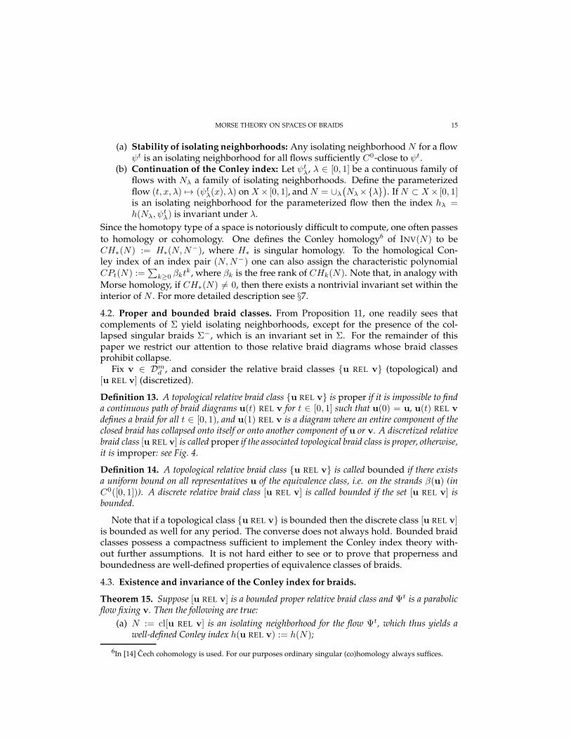
(a) Stability of isolating neighborhoods: Any isolating neighborhood N for a flowψt is an isolating neighborhood for all flows sufficiently C0-close to ψt.
(b) Continuation of the Conley index: Let ψtλ, λ ∈ [0, 1] be a continuous family of
flows with Nλ a family of isolating neighborhoods. Define the parameterizedflow (t, x, λ) 7→ (ψt
λ(x), λ) on X× [0, 1], andN = ∪λ
(Nλ×λ
). IfN ⊂ X× [0, 1]
is an isolating neighborhood for the parameterized flow then the index hλ =h(Nλ, ψ
tλ) is invariant under λ.
Since the homotopy type of a space is notoriously difficult to compute, one often passes
to homology or cohomology. One defines the Conley homology6 of INV(N) to beCH∗(N) := H∗(N,N−), where H∗ is singular homology. To the homological Con-ley index of an index pair (N,N−) one can also assign the characteristic polynomialCPt(N) :=
∑k≥0 βkt
k, where βk is the free rank of CHk(N). Note that, in analogy with
Morse homology, if CH∗(N) 6= 0, then there exists a nontrivial invariant set within theinterior of N . For more detailed description see §7.
4.2. Proper and bounded braid classes. From Proposition 11, one readily sees thatcomplements of Σ yield isolating neighborhoods, except for the presence of the col-lapsed singular braids Σ−, which is an invariant set in Σ. For the remainder of thispaper we restrict our attention to those relative braid diagrams whose braid classesprohibit collapse.
Fix v ∈ Dmd , and consider the relative braid classes u REL v (topological) and
[u REL v] (discretized).
Definition 13. A topological relative braid class u REL v is proper if it is impossible to finda continuous path of braid diagrams u(t) REL v for t ∈ [0, 1] such that u(0) = u, u(t) REL v
defines a braid for all t ∈ [0, 1), and u(1) REL v is a diagram where an entire component of theclosed braid has collapsed onto itself or onto another component of u or v. A discretized relativebraid class [u REL v] is called proper if the associated topological braid class is proper, otherwise,it is improper: see Fig. 4.
Definition 14. A topological relative braid class u REL v is called bounded if there existsa uniform bound on all representatives u of the equivalence class, i.e. on the strands β(u) (inC0([0, 1])). A discrete relative braid class [u REL v] is called bounded if the set [u REL v] isbounded.
Note that if a topological class u REL v is bounded then the discrete class [u REL v]is bounded as well for any period. The converse does not always hold. Bounded braidclasses possess a compactness sufficient to implement the Conley index theory with-out further assumptions. It is not hard either to see or to prove that properness andboundedness are well-defined properties of equivalence classes of braids.
4.3. Existence and invariance of the Conley index for braids.
Theorem 15. Suppose [u REL v] is a bounded proper relative braid class and Ψt is a parabolicflow fixing v. Then the following are true:
(a) N := cl[u REL v] is an isolating neighborhood for the flow Ψt, which thus yields awell-defined Conley index h(u REL v) := h(N);
6In [14] Cech cohomology is used. For our purposes ordinary singular (co)homology always suffices.

16 R.W. GHRIST, J.B. VAN DEN BERG, AND R.C. VANDERVORST
b b b b b
b b b b b
b b b b b
b b b b b
b b b b b
b b b b b
b b b b b
b b b b b
b
b
b
b
b b
b
b
b
b
FIGURE 4. Improper [left] and proper [right] relative braid classes.Both are bounded.
(b) The index h(u REL v) is independent of the choice of parabolic flow Ψt so long asΨt(v) = v;
(c) The index h(u REL v) is an invariant of[u REL [v]
].
Definition 16. The homotopy index of a bounded proper discretized braid class[u REL [v]
]
in Dnd REL [v] is defined to be h(u REL v), the Conley index of the braid class [u REL v] with
respect to some (hence any) parabolic flow fixing any representative v of the skeletal braid classπ[u REL [v]
]⊂ [v].
Proof. Isolation is proved by examining Ψt on the boundary ∂N . By Definition 13and 14 the set N is compact, and ∂N ⊂ Σ\Σ−. Choose a point u on ∂N . Proposition 11implies that the parabolic flow Ψt locally intersects ∂N at u alone and that furthermoreits length in the braid group strictly decreases. This implies that under Ψt, the point uexits the set N either in forwards or backwards time (if not both). Thus, u 6∈ INV(N)and (a) is proved.
Denote by h(u REL v) the index of INV(N). To demonstrate (b), consider two par-abolic flows Ψt
0 and Ψt1 that satisfy all our requirements, and consider the isolating
neighborhood N valid for both flows. Construct a homotopy Ψtλ, λ ∈ [0, 1], by con-
sidering the parabolic recurrence functions Rλ = (1 − λ)R0 + λR1, where R0 and R1
give rise to the flows Ψt0 and Ψt
1 respectively. It follows immediately that Ψtλ(v) = v,
for all λ ∈ [0, 1]; therefore N is an isolating neighborhood for Ψtλ with λ ∈ [0, 1]. Define
INVλ(N), λ ∈ [0, 1], to be the maximal invariant set in N with respect to the flow Ψtλ.
The continuation property of the Conley index completes the proof of (b).Assume that [u REL v] ∼ [u′ REL v′], so that there is a continuous path (u(λ),v(λ)),
for 0 ≤ λ ≤ 1, of braid pairs within Dn+md between the two. From the proof of Lemma 57
in Appendix A, there exists a continuous family of flows Ψtλ, such that Ψt
λ(v(λ)) = v(λ),for all λ ∈ [0, 1]. Item (a) ensures that Nλ := cl[u REL v(λ)] is an isolating neighborhoodfor all λ ∈ [0, 1]. The continuity of v(λ) implies that the set N := ∪λ
(Nλ × λ
)⊂
Dnd × [0, 1] is an isolating neighborhood for the parameterized flow (Ψt
λ(u), λ) on Dnd ×
[0, 1]. Therefore via the continuation property of the Conley index, h(u REL v(λ)) isindependent of λ ∈ [0, 1], which completes the proof of Item (c).
4.4. An intrinsic definition. For any bounded proper relative braid class [u REL v] wecan define its index intrinsically, independent of any notions of parabolic flows. Denoteas before byN the set cl[u REL v] within Dn
d . The singular braid diagrams Σ partition Dnd

MORSE THEORY ON SPACES OF BRAIDS 17
into disjoint cells (the discretized relative braid classes), the closures of which containportions of Σ. For a bounded proper braid class, N is compact, and ∂N avoids Σ−.
To define the exit set N−, consider any point w on ∂N ⊂ Σ. There exists a smallneighborhood W of w in Dn
d for which the subset W − Σ consists of a finite number ofconnected components Wj. Assume that W0 =W ∩N . We define N− to be the set ofw for which the word metric is locally maximal on W0, namely,
(15) N− := clw ∈ ∂N : |W0|word ≥ |Wj |word
∀j > 0.
We deduce that (N,N−) is an index pair for any parabolic flow for which Ψt(v) = v,and thus by the independence of Ψt, the homotopy type
[N/N−] gives the Conley in-
dex. The index can be computed by choosing a representative v ∈ [v] and determiningN and N−. A rigorous computer assisted approach exists for computing the homologi-cal index using cube complexes and digital homology [23].
4.5. Three simple examples. It is not obvious what the homotopy index is measuringtopologically. Since the space N has one dimension per free anchor point, examplesquickly become complex.
Example 1: Consider the proper period-2 braid illustrated in Fig. 5[left]. (Note thatdeleting any strand in the skeleton yields an improper braid.) There is exactly one freestrand with two anchor points (recall that these are closed braids and the left and rightsides are identified). The anchor point in the middle, u1, is free to move vertically be-tween the fixed points on the skeleton. At the endpoints, one has a singular braid in Σwhich is on the exit set since a slight perturbation sends this singular braid to a differ-ent braid class with fewer crossings. The end anchor point, u2 (= u0) can freely movevertically in between the two fixed points on the skeleton. The singular boundaries arein this case not on the exit set since pushing u2 across the skeleton increases the numberof crossings.
PSfrag replacementsu0
u1
u2
u2
u1
Σ
⊂
FIGURE 5. The braid of Example 1 [left] and the associated configura-tion space with parabolic flow [middle]. On the right is an expandedview of D1
2 REL v where the fixed points of the flow correspond to thefour fixed strands in the skeleton v. The braid classes adjacent to thesefixed points are not proper.
Since the points u1 and u2 can be moved independently, the configuration spaceN inthis case is the product of two compact intervals. The exit setN− consists of those points

18 R.W. GHRIST, J.B. VAN DEN BERG, AND R.C. VANDERVORST
on ∂N for which u1 is a boundary point. Thus, the homotopy index of this relative braidis [N/N−] ≃ S1.
Example 2: Consider the proper relative braid presented in Fig. 6[left]. Since there isone free strand of period three, the configuration space N is determined by the vec-tor of positions (u0, u1, u2) of the anchor points. This example differs greatly from theprevious example. For instance, the point u0 (as represented in the figure) may passthrough the nearest strand of the skeleton above and below without changing the braidclass. The points u1 and u2 may not pass through any strands of the skeleton withoutchanging the braid class unless u0 has already passed through. In this case, either u1 oru2 (depending on whether the upper or lower strand is crossed) becomes free.
To simplify the analysis, consider (u0, u1, u2) as all of R3 (allowing for the momentsingular braids and other braid classes as well). The position of the skeleton induces acubical partition of R3 by planes, the equations being ui = vαi for the various strandsvα of the skeleton v. The braid class N is thus some collection of cubes in R3. InFig. 6[right], we illustrate this cube complex associated to N , claiming that it is homeo-morphic to D2 × S1. In this case, the exit set N− happens to be the entire boundary ∂Nand the quotient space is homotopic to the wedge-sum S2 ∨ S3.
PSfrag replacements u0
u1
u2
u3
FIGURE 6. The braid of Example 2 and the configuration space N .
Example 3: To introduce the spirit behind the forcing theorems of the latter half ofthe paper, we reconsider the period two braid of Example 1. Take an n-fold cover ofthe skeleton as illustrated in Fig. 7. By weaving a single free strand in and out of thestrands as shown, it is possible to generate numerous examples with nontrivial index. Amoment’s meditation suffices to show that the configuration spaceN for this lifted braidis a product of 2n intervals, the exit set being completely determined by the numberof times the free strand is “threaded” through the inner loops of the skeletal braid asshown.
For an n-fold cover with one free strand we can select a family of 3n possible braidclasses describes as follows: the even anchor points of the free strand are always in themiddle, while for the odd anchor points there are three possible choices. Two of thesebraid classes are not proper. All of the remaining 3n − 2 braid classes are bounded andhave homotopy indices equal to a sphere Sk for some 0 ≤ k ≤ n. Several of these

MORSE THEORY ON SPACES OF BRAIDS 19
strands may be superimposed while maintaining a nontrivial homotopy index for thenet braid: we leave it to the reader to consider this interesting situation.
FIGURE 7. The lifted skeleton of Example 1 with one free strand.
Stronger results follow from projecting these covers back down to the period twosetting of Example 1. If the free strand in the cover is chosen not to be isotopic to aperiodic braid, then it can be shown via a simple argument that some projection ofthe free strand down to the period two case has nontrivial homotopy index. Thus, thesimple period two skeleton of Example 1 is the seed for an infinite number of braidclasses with nontrivial homotopy indices. Using the techniques of [32], one can use thisfact to show that any parabolic recurrence relation (R = 0) admitting this skeleton isforced to have positive topological entropy: cf. the related results from the Nielsen-Thurston theory of disc homeomorphisms [9].
5. STABILIZATION AND INVARIANCE
5.1. Free braid classes and the extension operator. Via the results of the previous sec-tion, the homotopy index is an invariant of the discretized braid class: keeping the periodfixed and moving within a connected component of the space of relative discretizedbraids leaves the index invariant. The topological braid class, as defined in §2, does nothave an implicit notion of period. The effect of refining the discretization of a topolog-ical closed braid is not obvious: not only does the dimension of the index pair change,the homotopy types of the isolating neighborhood and the exit set may change as wellupon changing the discretization. It is thus perhaps remarkable that any changes arecorrelated under the quotient operation: the homotopy index is an invariant of the topo-logical closed braid class.
On the other hand, given a complicated braid, it is intuitively obvious that a certainnumber of discretization points are necessary to capture the topology correctly. If theperiod d is too small Dn
d REL v may contain more than one path component with thesame topological braid class:
Definition 17. A relative braid class [u REL v] in Dnd REL v is called free if
(16) (Dnd REL v) ∩ u REL v = [u REL v];
that is, if any other discretized braid in Dnd REL v which has the same topological braid class as
u REL v is in the same discretized braid class [u REL v].
20 R.W. GHRIST, J.B. VAN DEN BERG, AND R.C. VANDERVORST
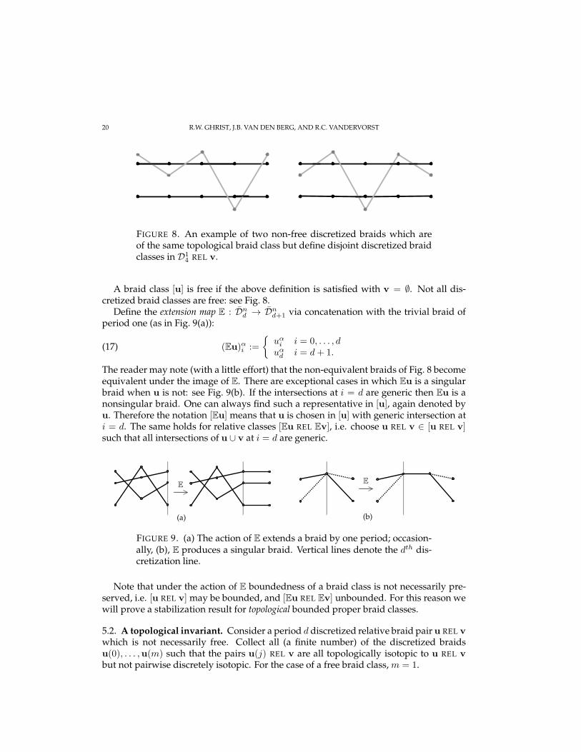
FIGURE 8. An example of two non-free discretized braids which areof the same topological braid class but define disjoint discretized braidclasses in D1
4 REL v.
A braid class [u] is free if the above definition is satisfied with v = ∅. Not all dis-cretized braid classes are free: see Fig. 8.
Define the extension map E : Dnd → Dn
d+1 via concatenation with the trivial braid ofperiod one (as in Fig. 9(a)):
(17) (Eu)αi :=
uαi i = 0, . . . , duαd i = d+ 1.
The reader may note (with a little effort) that the non-equivalent braids of Fig. 8 becomeequivalent under the image of E. There are exceptional cases in which Eu is a singularbraid when u is not: see Fig. 9(b). If the intersections at i = d are generic then Eu is anonsingular braid. One can always find such a representative in [u], again denoted byu. Therefore the notation [Eu] means that u is chosen in [u] with generic intersection ati = d. The same holds for relative classes [Eu REL Ev], i.e. choose u REL v ∈ [u REL v]such that all intersections of u ∪ v at i = d are generic.
PSfrag replacements
(a) (b)
EE
FIGURE 9. (a) The action of E extends a braid by one period; occasion-ally, (b), E produces a singular braid. Vertical lines denote the dth dis-cretization line.
Note that under the action of E boundedness of a braid class is not necessarily pre-served, i.e. [u REL v] may be bounded, and [Eu REL Ev] unbounded. For this reason wewill prove a stabilization result for topological bounded proper braid classes.
5.2. A topological invariant. Consider a period d discretized relative braid pair u REL v
which is not necessarily free. Collect all (a finite number) of the discretized braidsu(0), . . . ,u(m) such that the pairs u(j) REL v are all topologically isotopic to u REL v
but not pairwise discretely isotopic. For the case of a free braid class, m = 1.

MORSE THEORY ON SPACES OF BRAIDS 21
Definition 18. Given u REL v and u(0), . . . ,u(m) as above, denote by H(u REL v) the wedgeof the homotopy indices of these representatives,
(18) H(u REL v) :=
md∨
j=0
h(u(j) REL v),
where ∨ is the topological wedge which, in this context, identifies all the constituent exit sets toa single point.
This wedge product is well-defined by Theorem 15 by considering the isolatingneighborhood N = ∪jcl[u(j) REL v]. In general a union of isolating neighborhoodsis not necessarily an isolating neighborhood again. However, since the word metricstrictly decreases at Σ the invariant set decomposes into the union of invariant sets ofthe individual components of N . Indeed, if an orbit intersects two components it musthave passed through Σ: contradiction.
The principal topological result of this paper is that H is an invariant of the topologicalbounded proper braid class
u REL v
.
Theorem 19. Given u REL v ∈ Dnd REL v and u REL v ∈ Dn
dREL v which are topologically
isotopic as bounded proper braid pairs, then
(19) H(u REL v) = H(u REL v).
The key ingredients in this proof are that (1) the homotopy index is invariant un-der E (Theorem 19); and (2) discretized braids “converge” to topological braids undersufficiently many applications of E (Proposition 27).
Theorem 20. For u REL v any bounded proper discretized braid pair, the wedged homotopyindex of Definition 18 is invariant under the extension operator:
(20) H(Eu REL Ev) = H(u REL v).
Proof. By the invariance of the index with respect to the skeleton v, we may assume
that v is chosen to have all intersections generic (vαi 6= vα′
i for all strands α 6= α′). Thus,from the proof of Lemma 55 in Appendix A, we may fix a recurrence relation R havingv as fixed point(s) for which ∂1R0 = 0.
For ǫ > 0 consider the one-parameter family of augmented recurrence functions7
Rǫ = (Rǫi)
di=0 on braids of period d+ 1:
(21)Rǫ
i(uαi−1, u
αi , u
αi+1) := Ri(u
αi−1, u
αi , u
αi+1), i = 0, .., d− 1,
ǫ · Rǫd(u
αd−1, u
αd , u
αd+1) := uαd+1 − uαd .
Because of our choice of R0(r, s, t) = R0(s, t) as being independent of the first variable,
Rǫ0 is decoupled from the extension of the braid as uαd+1 wraps around to u
τ(α)0 . By
construction the above system satisfies Axioms (A1)-(A2) for all ǫ > 0 with, in particular,the strict monotonicity of (A1) holding only on one side. One therefore has a parabolicflow Ψt
ǫ on Dnd+1 for all ǫ > 0. In the singular limit ǫ = 0, this forces uαd = uαd+1, and one
obtains the flow Ψt0 = E Ψt.
7Recall the indexing conventions: for a period d+ 1 braid, uτ(α)0 = uα
d+1, and R0 := Rd+1.

22 R.W. GHRIST, J.B. VAN DEN BERG, AND R.C. VANDERVORST
Since the skeleton v has only generic intersections, Ev is a nonsingular braid. FromEquation (21), all stationary solutions of Ψt are stationary solutions for Ψt
ǫ, i.e., Ψtǫ(Ev) =
Ev, for all ǫ ≥ 0. Notice that this is not true in general for non-constant solutions.Denote by Bd+1 ⊂ Dn
d+1 REL Ev the subset of relative braids which are topologically
isotopic to Eu REL Ev. Likewise, denote by Bd ⊂ Dnd+1 the image under E of the subset
of braids in Dnd REL v which are topologically isotopic to u REL v. In other words,
(22) Bd+1 :=Eu REL Ev
∩ Dn
d+1 REL Ev ; Bd := E(
u REL v∩ Dn
d REL v).
As per the paragraph preceding Definition 18, there are a finite number of connectedcomponents of each of these sets. Clearly, Bd is a codimension-n subset of cl(Bd+1).Since not all braids in
u REL v
∩ Dn
d REL v have generic intersections, the set Bd maytangentially intersect the boundary of Bd+1. We will denote this set of E-singular braidsby ΣE := ∂Bd+1 ∩ Bd: see Fig. 10.
By performing an appropriate change of coordinates (cf. [12]), we can recast theparabolic system Rǫ as a singular perturbation problem. Let x = (xj)
ndj=1, with
xi+1+(α−1)d := uαi , and let y = (yα)nα=1, with yα := (uαd+1 − uαd ). Upon rescaling time as
τ := t/ǫ, the vector field induced by our choice of Rǫ is of the form
(23)dxdτ = ǫX(x,y),dydτ
= −y + ǫY (x),
for some (unspecified) vector fields X and Y with the functional dependence indicated.The product flow of this vector field (23) in the new coordinates is denoted by Φτ
ǫ and iswell-defined on Dn
d+1. In the case ǫ = 0, the set M := y = 0 ⊂ Dnd+1 is a submanifold
of fixed points containing Bd for which the flow Φτ0 is transversally nondegenerate (since
here y′ = −y). By construction cl(Bd) = cl(Bd+1) ∩M, as illustrated in Fig. 10 (in thesimple case where all braid classes are free and Bd+1 is thus connected).
The remainder of the analysis is a technique in singular perturbation theory fol-lowing [12]: one relates the τ -dynamics of Equation (23) to those of the t-dynamicson M, whose orbits are of the form (x(t), 0), where x(t) satisfies the limiting equationdx/dt = X(x, 0). The Conley index theory is well-suited to this situation.
For any compact set D ⊂ M and r ∈ R, let D(r) := (x,y) | (x, 0) ∈ D, ‖y‖ ≤ rdenote the “product” radius r neighborhood in Dn
d+1. Denote byC = C(D) the maximalvalue C := maxD ‖Y (x)‖. Due to the specific form of (23), we obtain the followinguniform squeezing lemma.
Lemma 21. If S is any invariant set of Φτǫ contained in some D(r), then in fact S ⊂ D(ǫC).
Moreover, for all points (x,y) with x ∈ D and ‖y‖ = 2ǫC it holds that ddτ ‖y‖ < 0.
Proof. Let (x,y)(τ) be an orbit in S contained in some D(r). Take the inner productof the y-equation with y:
〈dydτ,y〉(τ0) = −‖y(τ0)‖2 + ǫ〈Y (x(τ0)),y(τ0)〉,
≤ −‖y‖2 + ǫC‖y‖.

MORSE THEORY ON SPACES OF BRAIDS 23
PSfrag replacements
M
Σ
N0
D(r)
Bd+1
Bd
N0(2ǫC)
ΣE
K
FIGURE 10. The rescaled flow acts on Bd+1, the period d + 1 braidclasses. The submanifold M is a critical manifold of fixed points atǫ = 0. Any appropriate isolating neighborhood N0 in Bd thickens to anisolating neighborhood N0(2ǫC) which is not necessarily contained inBd+1.
Hence ddτ ‖y‖ ≤ −‖y‖+ ǫC, and we conclude that if ‖y(τ0)‖ > ǫC for some τ0 ∈ R, then
ddτ ‖y‖ < 0. Consequently ‖y(τ)‖ grows unbounded for τ < τ0 and therefore (x,y) 6∈ S,a contradiction. Thus ‖y(τ)‖ ≤ ǫC for all τ ∈ R.
For points (x,y) with x ∈ D and ‖y‖ = 2ǫC, the above inequality gives that ddτ ‖y‖ ≤
−‖y‖+ ǫC < 0.
By compactness of the proper braid class, it is clear that Bd+1, and thus the maximal
isolated invariant set of Φτǫ given by Sǫ := INV(Bd+1,Φ
τǫ )
8, is strictly contained (and thusisolated) inD(r) for some compactD ⊂ M and some r sufficiently large. FixC := C(D)as above. Lemma 21 now implies that as ǫ becomes small, Sǫ is squeezed into D(ǫC) —
a small neighborhood of a compact subset D of the critical manifold M, as in Fig. 10.9
This proximity of Sǫ to M allows one to compare the dynamics of the ǫ = 0 andǫ > 0 flows. Let N0 ⊂ Bd ⊂ M be an isolating neighborhood (isolating block withcorners) for the maximal t-dynamics invariant set S0 := INV(Bd,Ψ
t0) within the braid
class Bd. Combining Lemma 21 above, Theorem 2.3C of [12], and the existence theoremsfor isolating blocks [60], one concludes that if (N0, N
−0 ) is an index pair for the limiting
equations dx/dt = X(x, 0) then N0(2ǫC) is an isolating block for Φtǫ for 0 < ǫ ≤ ǫ∗(N0)
with ǫ∗ sufficiently small. A suitable index pair for the flow Φτǫ of Equation (23) is thus
given by
(24)(N0(2ǫC), N
−0 (2ǫC)
).
8Since Bd+1 is a proper braid class Sǫ is contained in its interior.9 If one applies singular perturbation theory it is possible to construct an invariant manifold Mǫ ⊂ D(ǫC).
The manifold Mǫ lies strictly within Bd+1 and intersects M at rest points of the Φt0.

24 R.W. GHRIST, J.B. VAN DEN BERG, AND R.C. VANDERVORST
Clearly, then, the homotopy index of S0 is equal to the homotopy index of INV(N0(2ǫC))for all ǫ sufficiently small. It remains to show that this captures the maximal invariantset Sǫ.
Lemma 22. For all sufficiently small ǫ, INV(N0(2ǫC),Φτǫ ) = Sǫ.
Proof. By the choice of D it holds that Sǫ ⊂ D(2ǫC). We start by proving that Sǫ ⊂N0(2ǫC) for ǫ sufficiently small. Assume by contradiction that Sǫj 6⊂ N0(2ǫjC) for somesequence ǫj → 0. Then, since N0(2ǫC) is an isolating neighborhood for ǫ ≤ ǫ∗, thereexist orbits (xǫj ,yǫj ) in Sǫj such that (xǫj ,yǫj )(τj) ∈ D(2ǫjC) − N0(2ǫjC), for someτj ∈ R. Define (xǫj , yǫj )(τ) = (xǫj ,yǫj )(τ − τj), and set (aǫj ,bǫj)(t) = (xǫj , yǫj )(τ). Thesequence (aǫj ,bǫj ) satisfies the equations
(25)d
dtaǫj = X(aǫj ,bǫj ),
d
dtbǫj = −1
ǫbǫj + Y (aǫj ).
By assumption ‖bǫj(t)‖ ≤ Cǫj , and ‖aǫj‖, ‖daǫj/dt‖ ≤ C, for all t ∈ R and allǫj . An Arzela-Ascoli argument then yields the existence of an orbit (a∗(t), 0) ⊂ Bd,
with (a∗(0), 0) ∈ cl(Bd − N0), satisfying the equation da∗
dt = X(a∗, 0). By defini-tion, (a∗, 0) ∈ INV(Bd) = INV(N0) ⊂ int(N0), a contradiction, which proves thatSǫ ⊂ N0(2ǫC) for ǫ sufficiently small.
The boundary of N0(2ǫC) splits as b1 ∪ b2, with
b1 = (x,y) | ‖y‖ = 2ǫC, and b2 = (x,y) | x ∈ ∂N0.Since the compact set N0 is contained in Bd, the boundary component b2 is contained inBd+1 provided that ǫ is sufficiently small. If the set ΣE is non-empty then the boundarycomponent b1 never lies entirely in Bd+1 regardless of ǫ. As ǫ → 0 the set N0(2ǫC) −(Bd+1∩N0(2ǫC)
)is contained is arbitrary small neighborhood of ΣE. Independent of the
parabolic flow in question, and thus of ǫ, there exists a neighborhood K ⊂ Σnd+1 REL v
of ΣE on which the co-orientation of the boundary is pointed inside the braid class Bd+1.In other words for every parabolic system the points inK enter Bd+1 under the flow, see
Fig. 11. By using coordinates uαi − uα′
i and uαi+1 − uα′
i+1 adapted to the singular strands,it it easily seen (Fig. 11) that the braids are simplified by moving into the set Bd+1.
We now show that INV(N0(2ǫC)) ⊂ Bd+1 ∩ N0(2ǫC). If not, then there exist points(xǫj ,yǫj ) ∈
[N0(2ǫjC)−
(Bd+1∩N0(2ǫjC)
)]∩ INV(N0(2ǫjC)) for some sequence ǫj → 0.
Consider the α-limit sets αǫj ((xǫj ,yǫj )). Since (xǫj ,yǫj ) ∈ INV(N0(2ǫjC)), and sinceΦτ
ǫj ((xǫj ,yǫj )) cannot enter Bd+1∩N0(2ǫjC) in backward time due to the co-orientation
of K , it follows that αǫj ((xǫj ,yǫj )) is contained in N0(2ǫjC)−(Bd+1 ∩N0(2ǫjC)
).
By a similar Arzela-Ascoli argument as before, this yields a set α0 ⊂ ΣE which isinvariant for the flow Ψt
0. However due to the form of the vector field the associatedflow Ψt
0 cannot contain an invariant set in ΣE, which proves that INV(N0(2ǫC)) ⊂ Bd+1∩N0(2ǫC) for ǫ sufficiently small.
Finally, knowing that Sǫ ⊂ INV(N0(2ǫC)), and that for sufficiently small ǫ it holdsINV(N0(2ǫC) = INV(Bd+1 ∩ N0(2ǫC)) = Sǫ, it follows that Sǫ = INV(N0(2ǫC)), whichproves the lemma.
Theorem 20 now follows. Since, by Theorem 15, the homotopy index is independentof the parabolic flow used to compute it, one may choose the parabolic flow Φτ
ǫ for ǫ > 0sufficiently small. The homotopy index of Φτ
ǫ on the maximal invariant set Sǫ yields the

MORSE THEORY ON SPACES OF BRAIDS 25
PSfrag replacements
uαi − uα′i
uαi+1 − u
α′i+1
FIGURE 11. The local picture of a generic singular tangency betweenstrands α (solid) and α′ (dashed). The shaded region represents Bd+1.
wedge of all the connected components: H(Eu REL Ev). We have computed that thisindex is equal to the index of Ψt on the original braid class: H(u REL v).
Remark 23. The proof of Theorem 20 implies that any component of the period-(d+ 1)braid class Bd+1 which does not intersect M must necessarily have trivial index.
Remark 24. The above procedure also yields a stabilization result for bounded properclasses which are not bounded as topological classes. In this case one simply augmentsthe skeleton v by two constant strands as follows. Define the augmented braid v∗ :=v ∪ v− ∪ v+, where
(26) v−i := minα,i
vαi − 1, v+i := maxα,i
vαi + 1.
Suppose [u REL v] ⊂ Dnd0
REL v is bounded for some period d0. It now holds that
h(u REL v) = h(u REL v∗), andu REL v∗
is a bounded class. It therefore follows
from Theorem 19 thatmd0∨
j=0
h(u(j) REL v
)= H(u REL v∗),(27)
where H can be evaluated via any discrete representative ofu REL v∗
of any ad-
missible period.
5.3. Eventually free classes. At the end of this subsection, we complete the proof ofTheorem 19. The preliminary step is to show that discretized braid classes are eventu-ally free under E.
Given a braid u ∈ Dnd , consider the extension Eu of period d + 1. Assume at first
the simple case in which d = 1, so that Eu is a period-2 braid. Draw the braid diagramβ(Eu) as defined in §2 in the domain [0, 2]×R. Choose any 1-parameter family of curves
γs : t 7→ (fs(t), t) ∈ (0, 2)×R such that γ0 : t 7→ (1, t) and so that γs is transverse10 to the
10At the anchor points, the transversality should be topological as opposed to smooth.

26 R.W. GHRIST, J.B. VAN DEN BERG, AND R.C. VANDERVORST
braid diagram β(Eu) for all s. Define the braid γs · Eu as follows:
(28) (γs · Eu)αi :=
(Eu)αi : i = 0, 2
γs ∩ (Eu)α : i = 1.
The point γs ∩ (Eu)α is well-defined since γs is always transverse to the braid strandsand γ0 intersects each strand but once.
Lemma 25. For any such family of curves γs, [γs · Eu] = [Eu].
Proof. It suffices to show that this path of braids does not intersect the singular braidsΣ. Since u is assumed to be a nonsingular braid, every crossing of two strands in thebraid diagram of Eu is a transversal crossing between i = 0 and i = 1. Thus, if for some
s, γs(t) ∩ (Eu)α = γs(t) ∩ (Eu)α′
for distinct strands α and α′, then
(29)(Euα
0 − Euα′
0
)(Euα
1 − Euα′
1
)< 0.
The braid γs · Eu has a crossing of the α and α′ strands at i = 1. Checking the transver-sality of this crossing yields
(30)
((γs · Eu)α0 − (γs · Eu)α
′
0
)((γs · Eu)α2 − (γs · Eu)α
′
2
)
=((Eu)α0 − (Eu)α
′
0
)((Eu)α2 − (Eu)α
′
2
)
=((Eu)α0 − (Eu)α
′
0
)((Eu)α1 − (Eu)α
′
1
)< 0.
Thus the crossing is transverse and the braid is never singular.
Note that the proof of Lemma 25 does not require the braid Eu to be a closed braiddiagram since the isotopy fixes the endpoints: the proof is equally valid for any localizedregion of a braid in which one spatial segment has crossings and the next segment hasflat strands.
Corollary 26. The “shifted” extension operator which inserts a trivial period-1 braid at the ith
discretization point in a braid has the same action on components of Dd as does E.
PSfrag replacements
σi σiσj σjσiσiσi σi+1σi+1σi+1
FIGURE 12. Relations in the braid group via discrete isotopy.
Proposition 27. The period-d discretized braid class [u] is free when d > |u|word.

MORSE THEORY ON SPACES OF BRAIDS 27
Proof. We must show that any braid u′ ∈ Dnd which has the same topological type as
u is discretely isotopic to u. Place both u and u′ in general position so as to record thesequences of crossings using the generators of the n-strand positive braid semigroup,σi, as in §2. Recall the braid group has relations σiσj = σjσi for |i − j| > 1 andσiσi+1σi = σi+1σiσi+1; closure requires making conjugacy classes equivalent.
The conjugacy relation can be realized by a discrete isotopy as follows: since d >|u|word, u must possess some discretization interval on which there are no crossings.Lemma 25 then implies that this interval without crossings commutes with all neighbor-ing discretization intervals via discrete isotopies. Performing d consecutive exchangesshifts the entire braid over by one discretization interval. This generates the conjugacyrelation.
To realize the remaining braid relations in a discrete isotopy, assume first that u andu′ are of the form that there is at most one crossing per discretization interval. It is theneasy to see from Fig. 12 that the braid relations can be executed via discrete isotopy.
In the case where u (and/or u′) exhibits multiple crossings on some discretizationintervals, it must be the case that a corresponding number of other discretization in-tervals do not possess any crossings (since d > |u|word). Again, by inductively utilizingLemma 25, we may redistribute the intervals-without-crossing and “comb” out the mul-tiple crossings via discrete isotopies so as to have at most one crossing per discretizationinterval.
Proof of Theorem 19: Assume thatu REL v
=u′ REL v′
. This implies that
there is a path of topological braid diagrams taking the pair (u,v) to (u′,v′). Thispath may be chosen so as to follow a sequence of standard relations for closed braids.From the proof of Proposition 27, these relations may be performed by a discretizedisotopy to connect the pair (Eju,Ejv) to (Eku′,Ekv′) for j and k sufficiently large, andof the right relative size to make the periods of both pairs equal. For this choice, then,[Eju REL [Ejv]
]=[Eku′ REL [Ekv′]
], and their homotopy indices agree. An application
of Theorem 20 completes the proof.
We suspect that all braids in the image of E are free: a result which, if true, wouldsimplify index computations yet further.
6. DUALITY
For purposes of computation of the index, we will often pass to the homologicallevel. In this setting, there is a natural duality made possible by the fact that the indexpair used to compute the index of a braid class can be chosen to be a manifold pair.
Definition 28. The duality operator on discretized braids is the map D : Dn2p → Dn
2p givenby
(31) (Du)αi := (−1)iuαi .
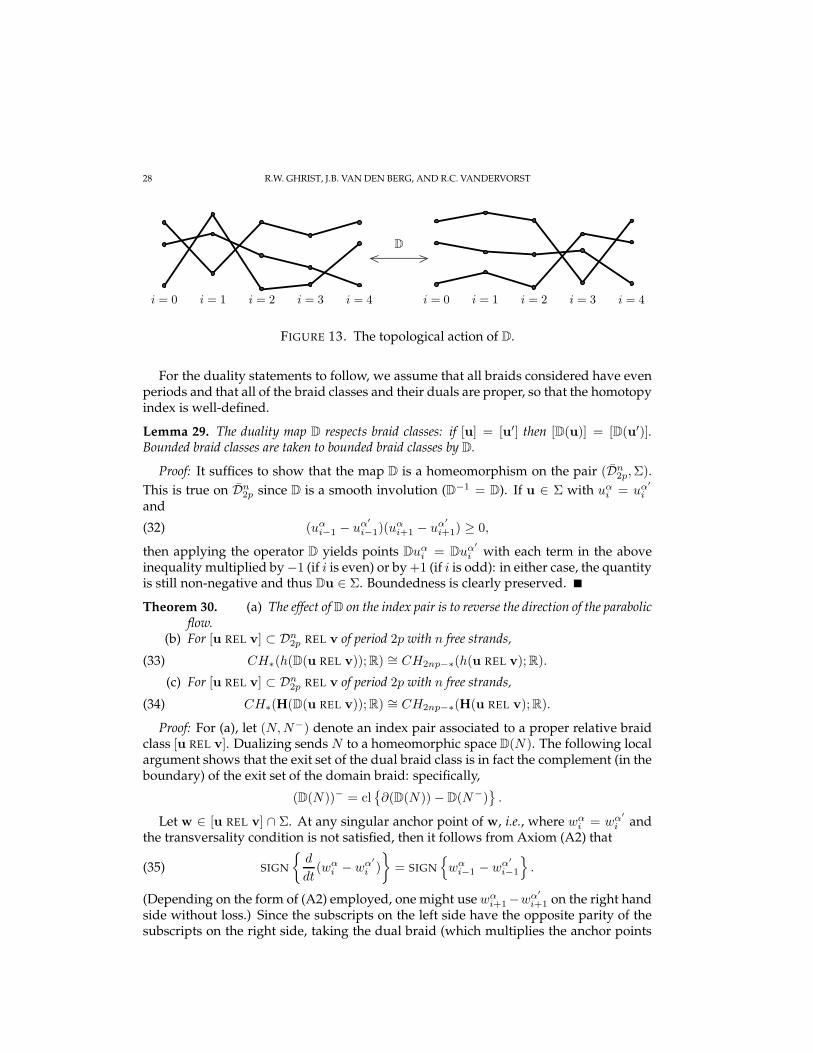
Clearly D induces a map on relative braid diagrams by defining D(u REL v) to beDu REL Dv. The topological action of D is to insert a half-twist at each spatial segmentof the braid. This has the effect of linking unlinked strands, and, sinceD is an involution,linked strands are unlinked by D: see Fig. 13.
28 R.W. GHRIST, J.B. VAN DEN BERG, AND R.C. VANDERVORST
PSfrag replacements
i = 0i = 0 i = 1i = 1 i = 2i = 2 i = 3i = 3 i = 4i = 4
D
FIGURE 13. The topological action of D.
For the duality statements to follow, we assume that all braids considered have evenperiods and that all of the braid classes and their duals are proper, so that the homotopyindex is well-defined.
Lemma 29. The duality map D respects braid classes: if [u] = [u′] then [D(u)] = [D(u′)].Bounded braid classes are taken to bounded braid classes by D.
Proof: It suffices to show that the map D is a homeomorphism on the pair (Dn2p,Σ).
This is true on Dn2p since D is a smooth involution (D−1 = D). If u ∈ Σ with uαi = uα
′
i
and
(32) (uαi−1 − uα′
i−1)(uαi+1 − uα
′
i+1) ≥ 0,
then applying the operator D yields points Duαi = Duα′
i with each term in the aboveinequality multiplied by −1 (if i is even) or by +1 (if i is odd): in either case, the quantityis still non-negative and thus Du ∈ Σ. Boundedness is clearly preserved.
Theorem 30. (a) The effect ofD on the index pair is to reverse the direction of the parabolicflow.
(b) For [u REL v] ⊂ Dn2p REL v of period 2p with n free strands,
(33) CH∗(h(D(u REL v));R) ∼= CH2np−∗(h(u REL v);R).
(c) For [u REL v] ⊂ Dn2p REL v of period 2p with n free strands,
(34) CH∗(H(D(u REL v));R) ∼= CH2np−∗(H(u REL v);R).
Proof: For (a), let (N,N−) denote an index pair associated to a proper relative braidclass [u REL v]. Dualizing sends N to a homeomorphic space D(N). The following localargument shows that the exit set of the dual braid class is in fact the complement (in theboundary) of the exit set of the domain braid: specifically,
(D(N))− = cl∂(D(N))− D(N−)
.
Let w ∈ [u REL v] ∩ Σ. At any singular anchor point of w, i.e., where wαi = wα′
i andthe transversality condition is not satisfied, then it follows from Axiom (A2) that
(35) SIGN
d
dt(wα
i − wα′
i )
= SIGN
wα
i−1 − wα′
i−1
.
(Depending on the form of (A2) employed, one might use wαi+1−wα′
i+1 on the right handside without loss.) Since the subscripts on the left side have the opposite parity of thesubscripts on the right side, taking the dual braid (which multiplies the anchor points

MORSE THEORY ON SPACES OF BRAIDS 29
by (−1)i and (−1)i−1 respectively) alters the sign of the terms. Thus, the operator Dreverses the direction of the parabolic flow.
From this, we may compute the Conley index of the dual braid by reversing the time-orientation of the flow. Since one can choose the index pair used to compute the indexto be an oriented manifold pair (specifically, an isolating block: see, e.g., [60]), one maythen apply a Poincare-Lefschetz duality argument as in [44] and use the fact that thedimension is 2np to obtain the duality formula for homology. This yields (b).
The final claim (c) follows from (b) by showing that D is bijective on topological braidclasses within Dn
2p. Assume that [u REL v] and [u′ REL v] are distinct braid classes inDn
2p of the same topological type. Since D is a homeomorphism on Dn2p, the dual classes
[Du REL Dv] and [Du′ REL Dv] are distinct. Claim (c) follows upon showing that theseduals are still topologically the same braid class.
Proposition 27 implies that [(E2ku) REL (E2kv)] = [(E2ku′) REL (E2kv)] for k suffi-ciently large since u REL v = u′ REL v. By Lemma 29,
D[(E2ku) REL (E2kv)
]= D
[(E2ku′) REL (E2kv)
],
which, by Lemma 7 means that these braids are topologically the same. The topologicalaction of dualizing the 2k-stabilizations of u REL v and u′ REL v is to add k full twists.Since the full twist is in the center of the braid group (this element commutes withall other elements of the braid group [8]), one can factor the dual braids within thetopological braid group and mod out by k full twists, yielding that Du REL Dv =Du′ REL Dv.
We use this homological duality to complete a crucial computation in the proof ofthe forcing theorems (e.g., Theorem 1) at the end of this paper. The following smallcorollary uses duality to give the first step towards answering the question of just whatthe homotopy index measures topologically about a braid class. Recall the definition ofan augmented braid from Remark 24.
Corollary 31. Consider the dual of any augmented proper relative braid. Adding a full twist tothis dual braid shifts the homology of the index up by two dimensions.
Proof: Assume that D[u REL v∗] is the dual of an augmented braid in period 2p (theaugmentation is required to keep the braid class bounded upon adding a full twist).The prior augmentation implies that the outer two strands of Dv “maximally link” theremainder of the relative braid. The effect of adding a full twist to this braid can berealized by instead stabilizing [u REL v∗] twice and then dualizing. The homologicalduality implies that for each connected component of the topological class,
(36)CH∗(h(DE2(u REL v∗))) ∼= CH2np+2−∗(h(E2(u REL v∗)))
∼= CH2np+2−∗(h(u REL v∗))∼= CH∗−2(h(D(u REL v∗))),
which gives the desired result for the index H via Theorem 30.
Remark 32. The homotopy version of (36) can be achieved by following a similar pro-cedure as in §5. One obtains a double-suspension of the homotopy index, as opposed toa shift in homology.

30 R.W. GHRIST, J.B. VAN DEN BERG, AND R.C. VANDERVORST
Remark 33. Given a braid class [u] of odd period p = 2d+ 1, the image under D is notnecessarily a discretized braid at all: without some symmetry condition, the braid willnot “close up” at the ends. To circumvent this, define the dual of u to be the braid D(u2)— the dual of the period 2p extension of u. The analogue of Theorem 30 above is that
(37) CH∗(H(SYM(D(u RELv)));R) ∼= CHnp−∗(H(u REL v);R),
where SYM denotes the subset of the braid class which consists of symmetric braids:uαi = uα2p−i for all i.
7. MORSE THEORY
It is clear that the Morse-theoretic content of the homotopy index on braids holdsimplications for the dynamics of parabolic flows and thus zeros of parabolic recurrencerelations. With this in mind, we restrict ourselves to bounded proper braid classes.
Recall that the characteristic polynomial of an index pair (N,N−) is the polynomial
(38) CPt(N) :=∑
k≥0
βktk; βk(N) := dimCHk(N ;R) = dimHk(N,N
−;R).
The Morse relations in the setting of the Conley index (see [14]) state that, if N has aMorse decomposition into distinct isolating subsets NaCa=1, then
(39)C∑
a=1
CPt(Na) = CPt(N) + (1 + t)Qt,
for some polynomial Qt with nonnegative integer coefficients.
7.1. The exact, nondegenerate case. For parabolic recurrence relations which satisfy(A3) (gradient type) it holds that if h(u REL v) 6= 0, then R has at least one fixed pointin [u REL v]. Indeed, one has:
Lemma 34. For an exact nondegenerate parabolic flow on a bounded proper relative braid class,the sum of the Betti numbers βk of h, as defined in (38), is a lower bound on the number of fixedpoints of the flow on that braid class.
Proof: The details of this standard Morse theory argument are provided for the sakeof completeness. Choose Ψt a nondegenerate gradient parabolic flow on [u REL v] (inparticular, Ψt fixes v for all time). Enumerate the [finite number of] fixed points uaCa=1
of Ψt on this [bounded] braid class. By nondegeneracy, the fixed point set may be takento be a Morse decomposition of INV(N). The characteristic polynomial of each fixed
point is merely tµ∗(ua), where µ∗(ua) is the Morse co-index of ua. Substituting t = 1
into Equation (39) yields the lower bound
(40) #Fix([u REL v],Ψt) ≥∑
k
βk(h).
On the level of the topological braid invariant H, one needs to sum over all the pathcomponents as follows. As in Theorem 19, choose period-d representatives u(j) (j from0 to m) for each path component of the topological class
u REL v
. If we consider

MORSE THEORY ON SPACES OF BRAIDS 31
fixed points in the union ∪mj=0[u(j) REL v], we obtain the following Morse inequalities
from (40) and Theorem 19:
(41) #Fix(∪mj=0[u(j) REL v],Ψt) ≥
∑
k
βk(H),
where βk(H) is the kth Betti number of H(u REL v∗). Thus, again, the sum of the Bettinumbers is a lower bound, with the proviso that some components may not contain anycritical points.
If the topological classu REL v
is bounded the inequality (41) holds with the
invariant H(u REL v).
7.2. The exact, degenerate case. Here a coarse lower bound still exists.
Lemma 35. For an arbitrary exact parabolic flow on a bounded relative braid class, the numberof fixed points is bounded below by the number of distinct nonzero monomials in the character-istic polynomial CPt(h).
Proof: Assuming that #Fix is finite, all critical points are isolated and form a Morsedecomposition of INV(N). The specific nature of parabolic recurrence relations revealsthat the dimension of the null space of the linearized matrix at an isolated critical pointis at most 2, see e.g. [56]. Using this fact Dancer proves [15], via the degenerate versionof the Morse lemma due to Gromoll and Meyer, that CHk(ua) 6= 0 for at most one indexk = k0. Equation (39) implies that,
(42)
Cd∑
a=1
CPt(ua) ≥ CPt(h)
on the level of polynomials. As the result of Dancer implies that for each a, CPt(ua) =Atk, for some A ≥ 0, it follows that the number of critical points needs to be at least thenumber of non-trivial monomials in CPt(h).
As before, if we instead use the topological invariant H foru REL v∗
we obtain
that the number of monomials in CPt(H) is a lower bound for the total sum of fixedpoints over the topologically equivalent path-components.
More elaborate estimates in some cases can be obtained via the extension of the Con-ley index due to Floer [17].
7.3. The non-exact case. If we consider parabolic recurrence relations that are not nec-essarily exact, the homotopy index may still provide information about solutions ofR = 0. This is more delicate because of the possibility of periodic solutions for the flowu′i = Ri(ui−1, ui, ui+1). For example, if CPt(h) mod (1 + t) = 0, the index does notprovide information about additional solutions for R = 0, as a simple counterexampleshows. However, if CPt(h) mod (1 + t) 6= 0, then there exists at least one solution ofR = 0 with the specified relative braid class. Specifically,
Lemma 36. An arbitrary parabolic flow on a bounded relative braid class is forced to have afixed point if χ(h) := CP−1(h) is nonzero. If the flow is nondegenerate, then the number offixed points is bounded below by the quantity
(43)(CPt(h) modZ+[t] (1 + t)
)∣∣t=1

32 R.W. GHRIST, J.B. VAN DEN BERG, AND R.C. VANDERVORST
Proof: Set N = cl([u REL v]). As the vector field R has no zeros at ∂N , the Brouwer
degree, deg(R, N, 0), may be computed via a small perturbation R and is given by11
deg(R, N, 0) :=∑
u∈N,R(u)=0
sign det(−dR(u)).
For a generic perturbation R the associated parabolic flow Ψt is a Morse-Smale flow
[21]. The (finite) collection of rest points ua and periodic orbits γb of Ψt then yieldsa Morse decomposition of Inv(N), and the Morse inequalities are
∑
a
CPt(ua) +∑
b
CPt(γb) = CPt(h) + (1 + t)Qt.
The indices of the fixed points are given by CPt(ua) = tµ∗(ua), where µ∗ is the number
of eigenvalues of dR(ua) with positive real part, and the indices of periodic orbits are
given by CPt(γb) = (1 + t)tµ∗(γb). Upon substitution of t = −1 we obtain
deg(R, N, 0) = deg(R, N, 0) =∑
a
(−1)µ∗(ua)
=∑
a
CP−1(ua) = CP−1(h) = χ(h).
Thus, if the Euler characteristic of h is non-trivial, then R has at least one zero in N .In the generic case the Morse relations give even more information. One has
CPt(h) = p1(t) + (1 + t)p2(t), with p1, p2 ∈ Z+[t], and CPt(h) modZ+[t] (1 + t) = p1(t).It then follows that
∑a CPt(ua) ≥ CPt(h) modZ+[t] (1 + t), proving the stated lower
bound.The obvious extension of these results to the full index H is left to the reader.
8. SECOND ORDER LAGRANGIAN SYSTEMS
In this final third of the paper, we apply the developed machinery to the prob-lem of forcing closed characteristics in second order Lagrangian systems of twist type.The vast literature on fourth order differential equations coming from second orderLagrangians includes many physical models in nonlinear elasticity, nonlinear optics,physics of solids, Ginzburg-Landau equations, etc. (see §1). In this context we mentionthe work of [1, 38, 49, 50].
8.1. Twist systems. We recall from §1 that closed characteristics at an energy level Eare concatenations of monotone laps between minima and maxima (ui)i∈Z, which areperiodic sequences with even period 2p. The extrema are restricted to the set UE , whoseconnected components are denoted by IE : interval components (see §1.2 for the precisedefinition). The problem of finding closed characteristics can, in most cases, be formu-lated as a finite dimensional variational problem on the extrema (ui). The followingtwist hypothesis, introduced in [58], is key:
(T): infJE[u] =∫ τ
0
(L(u, ux, uxx) + E
)dx |u ∈ Xτ (u1, u2), τ ∈ R+ has a minimizer
u(x;u1, u2) for all (u1, u2) ∈ IE × IE | u1 6= u2, and u and τ are C1-smoothfunctions of (u1, u2).
11We choose to define the degree via −dR in order to simplify the formulae.

MORSE THEORY ON SPACES OF BRAIDS 33
Here Xτ = Xτ (u1, u2) = u ∈ C2([0, τ ]) | u(0) = u1, u(τ) = u2, ux(0) = ux(τ) =0 and ux|(0,τ) > 0.
Hypothesis (T) is a weaker version of the hypothesis that assumes that the monotonelaps between extrema are unique (see, e.g., [34, 35, 58]). Hypothesis (T) is valid for largeclasses of Lagrangians L. For example, if L(u, v, w) = 1
2w2 +K(u, v), the following two
inequalities ensure the validity of (T):
(a) ∂K∂v v −K(u, v)− E ≤ 0, and
(b) ∂2K∂v2 |v|2 − 5
2
∂K∂v v −K(u, v)− E
≥ 0 for all u ∈ IE and v ∈ R.
Many physical models, such as the Swift-Hohenberg equation (3), meet these require-ments, although these conditions are not always met. In those cases numerical calcu-lations still predict the validity of (T), which leaves the impression that the results ob-tained for twist systems carry over to many more systems for which Hypothesis (T) is
hard to check.12 For these reasons twist systems play a important role in understandingsecond order Lagrangian systems. For a direct application of this see [31].
The existence of minimizing laps is valid under very mild hypotheses on K (see[31]). In that case (b) above is enough to guarantee the validity of (T). An example of aLagrangian that satisfies (T), but not (a) is given by the Erickson beam-model [30, 49, 55]
L(u, ux, uxx) =α2 |uxx|2 + 1
4 (|ux|2 − 1)2 + β2u
2.
8.2. Discretization of the variational principle. We commence by repeating the under-lying variational principle for obtaining closed characteristics as described in [58]. In thepresent context a broken geodesic is a C2-concatenation of monotone laps (alternating be-tween increasing and decreasing laps) given by Hypothesis (T). A closed characteristicu at energy level E is a (C2-smooth) function u : [0, τ ] → R, 0 < τ < ∞, which isstationary for the action JE [u] with respect to variations δu ∈ C2
per(0, τ), and δτ ∈ R+,and as such is a ‘smooth broken geodesic’.
The following result, a translation of results implicit in [58], is the motivation andbasis for the applications of the machinery in the first two-thirds of this paper.
Theorem 37. Extremal points ui for bounded solutions of second order Lagrangian twistsystems are solutions of an exact parabolic recurrence relation with the constraints that (i)(−1)iui < (−1)iui+1; and (ii) the recurrence relation blows up along any sequence satisfy-ing ui = ui+1.
Proof: For simplicity, we restrict to the case of a nonsingular energy level E: for sin-gular energy levels, a slightly more involved argument is required. Denote by I theinterior of IE , and by ∆(I) = ∆ := (u1, u2) ∈ I × I | u1 = u2 the diagonal. Thendefine the generating function
(44) S : (I × I)−∆ → R ; S(u1, u2) :=
∫ τ
0
(L(u, ux, uxx) + E
)dx;
the action of the minimizing lap from u1 to u2. That S is a well-defined function is thecontent of Hypothesis (T). The action functional associated to S for a period 2p system is
12Another method to implement the ideas used in this paper is to set up a curve-shortening flow for
second order Lagrangian systems in the (u, u′) plane.

34 R.W. GHRIST, J.B. VAN DEN BERG, AND R.C. VANDERVORST
the function
W2p(u) :=
2p−1∑
i=0
S(ui, ui+1).
Several properties of S follow from [58]:
(a) [smoothness] S ∈ C2(I × I\∆).(b) [monotonicity] ∂1∂2S(u1, u2) > 0 for all u1 6= u2 ∈ I .(c) [diagonal singularity] lim
u1րu2
−∂1S(u1, u2) = limu2ցu1
∂2S(u1, u2) =
limu1ցu2
∂1S(u1, u2) = limu2րu1
−∂2S(u1, u2) = +∞.
In general the function ∂1S(u1, u2) is strictly increasing in u2 for all u1 ≤ u2 ∈ IE , andsimilarly ∂2S(u1, u2) is strictly increasing in u1. The function S also has the additionalproperty that S|∆ ≡ 0.
Critical points of W2p satisfy the exact recurrence relation
Ri(ui−1, ui, ui+1) := ∂2S(ui−1, ui) + ∂1S(ui, ui+1) = 0,(45)
where Ri(r, s, t) is both well-defined and C1 on the domains
Ωi = (r, s, t) ∈ I3 | (−1)i+1(s− r) > 0, (−1)i+1(s− t) > 0,
by Property (a). The recurrence function R is periodic with d = 2, as are the domains
Ω.13 Property (b) implies that Axiom (A1) is satisfied. Indeed, ∂1Ri = ∂1∂2S(ui−1, ui) >0, and ∂3Ri = ∂1∂2S(ui, ui+1) > 0.
Property (c) provides information about the behavior of R at the diagonal boundariesof Ωi, namely,
(46)limsցr Ri(r, s, t) = limsցt Ri(r, s, t) = +∞limsրr Ri(r, s, t) = limsրt Ri(r, s, t) = −∞
The parabolic recurrence relations generated by second order Lagrangians are de-fined on the constrained polygonal domains Ωi.
Definition 38. A parabolic recurrence relation is said to be of up-down type if (46) is satisfied.
In the next subsection we demonstrate that the up-down recurrence relations can beembedded into the standard theory as developed in §2-§7.
8.3. Up-down restriction. The variational set-up for second order Lagrangians intro-duces a few complications into the scheme of parabolic recurrence relations as discussedin §2-§7. The problem of boundary conditions will be considered in the following sec-tion. Here, we retool the machinery to deal with the fact that maxima and minima are
forced to alternate. Such braids we call up-down braids.14
13We could also work with sequences u that satisfy (−1)i+1(ui+1 − ui) > 0.14The more natural term alternating has an entirely different meaning in knot theory.

MORSE THEORY ON SPACES OF BRAIDS 35
8.3.1. The space E .
Definition 39. The spaces of general/nonsingular/singular up-down braid diagrams are definedrespectively as:
En2p := Dn
2p ∩u : (−1)i
(uαi+1 − uαi
)> 0 ∀i, α
,
En2p := Dn
2p ∩u : (−1)i
(uαi+1 − uαi
)> 0 ∀i, α
,
ΣE := En2p − En
2p.
Path components of En2p comprise the up-down braid types [u]E , and path components in
En2p REL v comprise the relative up-down braid types [u REL v]E .
The set En2p has a boundary in Dn
2p
(47) ∂En2p = ∂
(Dn
2p ∩u : (−1)i
(uαi+1 − uαi
)≥ 0 ∀i, α
)
Such braids, called horizontal singularities, are not included in the definition of En2p since
the recurrence relation (45) does not induce a well-defined flow on the boundary ∂En2p.
Lemma 40. For any parabolic flow of up-down type on En2p, the flow blows up in a neighbor-
hood of ∂En2p in such a manner that the vector field points into En
2p. All of the conclusions of
Theorem 15 hold upon considering the ǫ-closure of braid classes [u REL v]E in En2p, denoted
clE,ǫ[u REL v]E :=u REL v ∈ clE [u REL v]E : (−1)i
(uαi+1 − uαi
)≥ ǫ ∀i, α
,
for all ǫ > 0 sufficiently small.
Proof: The proof that any parabolic flow Ψt of up-down type acts here so as to strictlydecrease the word metric at singular braids is the same proof as used in Proposition 11.The only difficulty arises in what happens at the boundary of En
2p: we must show that
Ψt respects the up-down restriction in forward time.Define the function
ǫ(u) = mini,α
|uαi − uαi+1|.
Clearly, if ǫ(u) = 0, then u ∈ ∂En2p. Let u ∈ En
2p, and consider the evolution Ψt(u), t > 0.
We compute ddtǫ(Ψ
t(u)) as ǫ(Ψt(u)) becomes small. Using (45) it follows that
d
dt(uαi − uαi+1) = Ri(u
αi−1, u
αi , u
αi+1)−Ri+1(u
αi , u
αi+1, u
αi+2) → ∞,
as ui ց ui+1, (i odd),
d
dt(uαi+1 − uαi ) = Ri+1(u
αi , u
αi+1, u
αi+2)−Ri(u
αi−1, u
αi , u
αi+1) → ∞,
as ui ր ui+1, (i even).
These inequalities show that ddtǫ(Ψ
t(u)) > 0 as soon as ǫ(Ψt(u)) becomes too small.
Due to the boundedness of [u REL v]E and the infinite repulsion at ∂En2p, we can choose
a uniform ǫ(u REL v) > 0 so that ddtǫ(Ψ
t(u)) > 0 for ǫ(Ψt(u)) ≤ ǫ(u REL v), and thusclE,ǫ[u REL v]E is an isolating neighborhood for all 0 < ǫ ≤ ǫ(u REL v).

36 R.W. GHRIST, J.B. VAN DEN BERG, AND R.C. VANDERVORST
8.3.2. Universality for up-down braids. We now show that the topological informationcontained in up-down braid classes can be continued to the canonical case describedin §2. As always, we restrict attention to proper, bounded braid classes, proper beingdefined as in Definition 13, and bounded meaning that the set [u REL v]E is boundedin Dn
2p. Note that an up-down braid class [u REL v]E can sometimes be bounded while[u REL v] is not. To bounded proper up-down braids we assign a homotopy index.From Lemma 40 it follows that for ǫ sufficiently small the set NE,ǫ := clE,ǫ[u REL v]E is
an isolating neighborhood in En2p whose Conley index,
h(u REL v, E) := h(NE,ǫ),
is well-defined with respect to any parabolic flow Ψt generated by a parabolic recur-rence relation of up-down type, and is independent of ǫ. As before, non-triviality ofh(NE,ǫ) implies existence of a non-trivial invariant set inside NE,ǫ (see §8.3.3).
The obvious question is what relationship holds between the homotopy indexh(u REL v, E) and that of a braid class without the up-down restriction. To answerthis, augment the skeleton v as follows: define v∗ = v ∪ v− ∪ v+, where
v−i := minα,i
vαi − 1 + (−1)i+1, v+i := maxα,i
vαi + 1 + (−1)i+1.
The topological braid class u REL v∗ is bounded and proper. Indeed, boundednessfollows from adding the strands v± which bound u, since minα,i v
αi ≤ uαi ≤ maxα,i v
αi .
Properness is satisfied since u REL v is proper.
Theorem 41. For any bounded proper up-down braid class [u REL v]E in En2p REL v,
h(u REL v, E) = h(u REL v∗).
Proof. From Lemma 55 in Appendix A we obtain a parabolic recurrence relation R0
(not necessarily up-down type) for which v∗ is a solution. We denote the associatedparabolic flow by Ψt
0. Define two functions k1 and k2 in C1(R), with k′1 ≥ 0 ≥ k′2, andk1(τ) = 0 for τ ≤ −2δ, k1(−δ) ≥ K , and k2(τ) = 0 for τ ≥ 2δ, k2(δ) ≥ K , for someδ > 0 and K > 0 to be specified later. Introduce a new recurrence function R1
i (r, s, t) =R0
i (r, s, t)+k2(s−r)+k1(t−s) for i odd, and R1i (r, s, t) = R0
i (r, s, t)−k1(s−r)−k2(t−s)for i even. The associated parabolic flow will be denoted by Ψt
1, and Ψt1(v
∗) = v∗
by construction by choosing δ sufficiently small. Indeed, if we choose δ < ǫ(v), theaugmented skeleton is a fixed point for Ψt
1.Since the braid class [u REL v∗] is bounded and proper, N1 = cl[u REL v∗] is an
isolating neighborhood with invariant set INV(N1). If we choose K large enough, andδ sufficiently small, then the invariant set INV(N1) lies entirely in clE,ǫ[u REL v∗]E =
clE,ǫ[u REL v]E = NE,ǫ. Indeed, for large K we have that for each i, R1i (r, s, t) has a
fixed sign on the complement of NE,ǫ. Therefore, h(u REL v∗) = h(N1) = h(NE,ǫ). Nowrestrict the flow Ψt
1 to NE,ǫ ⊂ En2p REL v. We may now construct a homotopy between
Ψt1 and Ψt, via (1 − λ)R + λR1 (see Appendix A), where R and the associated flow Ψt
are defined by (45). The braid v∗ is stationary along the homotopy and therefore
h(N1) = h(NE,ǫ,Ψt1) = h(NE,ǫ,Ψ
t),
which proves the theorem.

MORSE THEORY ON SPACES OF BRAIDS 37
We point out that similar results can be proved for other domains Ωi with variousboundary conditions. The key observation is that the up-down constraint is really justan addition to the braid skeleton.
8.3.3. Morse theory. For bounded proper up-down braid classes [u REL v]E the Morsetheory of §7 applies. Combining this with Lemma 40 and Theorem 41, the topologicalinformation is given by the invariant H of the topological braid type
u REL v∗
.
Corollary 42. On bounded proper up-down braid classes, the total number of fixed points of anexact parabolic up-down recurrence relation is bounded below by the number of monomials inthe critical polynomial CPt(H) of the homotopy index.
Proof. Since all critical point are contained in NE,ǫ the corollary follows from theLemmas 35, 40 and Theorem 41.
9. MULTIPLICITY OF CLOSED CHARACTERISTICS
We now have assembled the tools necessary to prove Theorem 1, the general forc-ing theorem for closed characteristics in terms of braids, and Theorems 2 and 3, theapplication to singular and near-singular energy levels. Given one or more closed char-acteristics, we keep track of the braiding of the associated strands, including at will anyperiod-two shifts. Fixing these strands as a skeleton, we add hypothetical free strandsand compute the homotopy index. If nonzero, this index then forces the existence ofthe free strand as an existing solution, which, when added to the skeleton, allows oneto iterate the argument with the goal of producing an infinite family of forced closedcharacteristics.
The following lemma (whose proof is straightforward and thus omitted) will be usedrepeatedly for proving existence of closed characteristics.
Lemma 43. Assume that R is a parabolic recurrence relation on Dnd with u a solution. Then,
for each integer N > 1, there exists a lifted parabolic recurrence relation on DnNd for which every
lift of u is a solution. Furthermore, any solution to the lifted dynamics on DnNd projects to some
period-d solution. 15
The primary difficulties in the proof of the forcing theorems are (i) computing theindex (we will use all features of the machinery developed thus far, including stabiliza-tion and duality); and (ii) asymptotics/boundary conditions related to the three typesof closed interval components IE : a compact interval, the entire real line, and the semi-infinite ray.
All of the forcing theorems are couched in a little braid-theoretic language:
Definition 44. The intersection number of two strands uα, uα′
of a braid u is the number ofcrossings in the braid diagram, denoted
ι(uα,uα′
) := # of crossings of strands
The trivial braid on n strands is any braid (topological or discrete) whose braid diagram has no
crossings whatsoever, i.e., ι(uα,uα′
) = 0, for all α, α′. The full-twist braid on n strands, is
15This does not imply a d-periodic solution, but merely a braid diagram u of period d.

38 R.W. GHRIST, J.B. VAN DEN BERG, AND R.C. VANDERVORST
the braid of n connected components, each of which has exactly two crossings with every other
strand, i.e., ι(uα,uα′
) = 2 for all α 6= α′.
Among discrete braids of period two, the trivial braid and the full twist are duals inthe sense of §6.
9.1. Compact interval components. Let E be a regular energy level for which the setUE contains a compact interval component IE .
Theorem 45. Suppose that a twist system with compact IE possesses one or more closed charac-teristics which, as a discrete braid diagram, form a nontrivial braid. Then there exists an infinityof non-simple, geometrically distinct closed characteristics in IE .
In preparation for the proof of Theorem 45 we state a technical lemma, whose [short]proof may be found in [58].
Lemma 46. Let IE = [u−, u+], then there exists a δ0 > 0 such that
(1) R1(u− + δ, u−, u− + δ) > 0, R1(u+, u+ − δ, u+) < 0, and(2) R2(u−, u− + δ, u−) > 0, R2(u+ − δ, u+, u+ − δ) < 0,
for any 0 < δ ≤ δ0.
Proof of Theorem 45. Via Theorem 37, finding closed characteristics is equivalent tosolving the recurrence relation given by (45). Define the domains
Ωδi =
(ui−1, ui, ui+1) ∈ I3E | u− + δ < ui±1 < ui − δ/2 < u+ − δ, i odd,(ui−1, ui, ui+1) ∈ I3E | u− + δ < ui + δ/2 < ui±1 < u+ − δ, i even,
For any integer p ≥ 1 denote by Ω2p the set of 2p-periodic sequences ui for which(ui−1, ui, ui+1) ∈ Ωδ
i . By Lemma 46, choosing 0 < δ < δ0 small enough forces the vectorfield R = (Ri) to be everywhere transverse to ∂Ω2p, making Ω2p positively invariant forthe induced parabolic flow Ψt.
By Lemma 43, one can lift the assumed solution(s) to a pair of period 2p single-stranded solutions to (45), v1 and v2, satisfying ι(v1,v2) 6= 0, for some p ≥ 1. Definethe cones
C− = u ∈ Ω2p | ui ≤ vαi , α = 1, 2, andC+ = u ∈ Ω2p | ui ≥ vαi , α = 1, 2.
The combination of the facts ι(v1,v2) = r > 0, Axiom (A1), and the behavior of Ron ∂Ω2p implies that on the boundaries of the cones C− and C+ the vector field R iseverywhere transverse and pointing inward. Therefore, C− and C+ are also positivelyinvariant with respect to the parabolic flow Ψt. Consequently, W2p has global max-ima v− and v+ on int(C−) and int(C+) respectively. The maxima v− and v+ have theproperty that v−i < vαi < v+i , α = 1, 2. As a braid diagram, v = v1,v2,v−,v+ is astationary skeleton for the induced parabolic flow Ψt.
Having found the solutions v− and v+ we now choose a compact interval I IE ,such that the skeletal strands are all contained in I . In this way we obtain a proper para-bolic flow (circumventing boundary singularities) which can be extended to a parabolicflow on E1
2p REL v. Let [u REL v]E be the relative braid class with a period 2p free strand
u = ui which links the strands v1 and v2 with intersection number 2q while satisfyingv−i < ui < v+i : see Fig. 14 below.

MORSE THEORY ON SPACES OF BRAIDS 39
PSfrag replacements
u
v1v2
v+
v−
FIGURE 14. A representative braid class for the compact case: q =1, r = 4, 2p = 6.
As an up-down braid class, [u REL v]E is a bounded proper braid class provided0 < 2q < r ≤ 2p, and the Morse theory discussed in §7 and §8.3.3 then requiresthe evaluation of the invariant H of the topological class
u REL v∗
. In this case,
since h(u REL v, E) = h(u REL v∗) = h(u REL v), augmentation is not needed, andH(u REL v∗) = H(u REL v). The nontriviality of the homotopy index H is given by thefollowing lemma, whose proof we delay until §10.
Lemma 47. The Conley homology of H(u REL v) is given by:
(48) CHk(H) =
R : k = 2q − 1, 2q0 : else.
In particular CPt(H) = t2q−1(1 + t).
From the Morse theory of Corollary 42 we derive that for each q satisfying 0 < 2q <r ≤ 2p there exist at least two distinct period-2p solutions of (45), which generically areof index 2q and 2q − 1. In this manner, the number of solutions depends on r and p.To construct infinitely many, we consider m-fold coverings of the skeleton v, i.e., oneperiodically extends v to a skeleton contained in E4
2pm, m ≥ 1. Now q must satisfy0 < 2q < rm ≤ 2pm. By choosing triples (q, p,m) such that (q, pm) are relative prime,we obtain the same Conley homology as above, and therefore an infinity of pairs ofgeometrically distinct solutions of (45), which, via Lemma 43 and Theorem 37 yield aninfinity of closed characteristics.
Note that if we set qm = q and pm = pm, then the admissible ratios qmpm
for finding
closed characteristics are determined by the relation
0 <qmpm
<r
2p.(49)
Thus if v1 and v2 are maximally linked, i.e. r = 2p, then closed characteristics exist forall ratios in Q ∩ (0, 1).
9.2. Non-compact interval components: IE = R. On non-compact interval compo-nents, closed characteristics need not exist. An easy example of such a system is givenby the quadratic Lagrangian L = 1
2 |uxx|2 + α2 |ux|2 + 1
2 |u|2, with α > −2. Clearly IE = Rfor all E > 0, and the Lagrangian system has no closed characteristics for those en-ergy levels. For α < −2 the existence of closed characteristics strongly depends on theeigenvalues of the linearization around 0. To treat non-compact interval components,
40 R.W. GHRIST, J.B. VAN DEN BERG, AND R.C. VANDERVORST
some prior knowledge about asymptotic behavior of the system is needed. We adopt anasymptotic condition shared by most physical Lagrangians: dissipativity.
Definition 48. A second order Lagrangian system is dissipative on an interval componentIE = R if there exist pairs u∗1 < u∗2, with −u∗1 and u∗2 arbitrarily large, such that
−∂1S(u∗1, u∗2) > 0, ∂2S(u∗1, u
∗2) > 0, and
∂1S(u∗2, u
∗1) > 0, −∂2S(u∗2, u∗1) > 0.
Dissipative Lagrangians admit a strong forcing theorem:
Theorem 49. Suppose that a dissipative twist system with IE = R possesses one or more closedcharacteristic(s) which, as discrete braid diagram in the period-two projection, forms a link whichis not a full-twist (Definition 44). Then there exists an infinity of non-simple, geometricallydistinct closed characteristics in IE .
Proof. After taking the p-fold covering of the period-two projection for some p ≥ 1,the hypotheses imply the existence two sequences v1 and v2 that form a braid diagramin E2
2p whose intersection number is not maximal, i.e. 0 ≤ ι(v1,v2) = r < 2p. Following
Definition 48, choose I = [u∗1, u∗2], with u∗1 < u∗2 such that u∗1 < v1i , v
2i < u∗2 for all i, and
let Ωδi and Ω2p be as in the proof of Theorem 45, with u∗1 and u∗2 playing the role of u−+δ
and u+ − δ respectively for some δ > 0 small. Furthermore define the set
C := u ∈ Ω2p | ι(u,v1) = ι(u,v2) = 2p.Since 0 ≤ ι(v1,v2) < 2p, the vector field R given by (45) is transverse to ∂C. Moreover,the set C is contractible, compact, and R is pointing outward at the boundary ∂C. Theset C is therefore negatively invariant for the induced parabolic flow Ψt. Consequently,there exists a global minimum v3 in the interior of C. Define the skeleton v to be v :=v1,v2,v3.
Consider the up-down relative braid class [u REL v]E described as follows: choose u
to be a 2p-periodic strand with (−1)iui ≥ (−1)iv3i , such that u has intersection number2q with each of the strands v1 ∪ v2, 0 ≤ r < 2q < 2p, as in Fig. 15. For p ≥ 2, [u REL v]Eis a bounded proper up-down braid class. As before, in order to apply the Morse theoryof Corollary 42, it suffices to compute the homology index of the topological braid classu REL v∗
:
Lemma 50. The Conley homology of H(u REL v∗) is given by:
(50) CHk(H) =
R : k = 2q, 2q + 10 : else
In particular CPt(H) = t2q(1 + t).
By the same covering/projection argument as in the proof of Theorem 45, infinitelymany solutions are constructed within the admissible ratios
r
2p<qmpm
< 1.(51)
Theorem 49 also implies that the existence of a single non-simple closed characteristicyields infinitely many other closed characteristics. In the case of two unlinked closedcharacteristics all possible ratios in Q ∩ (0, 1) can be realized.
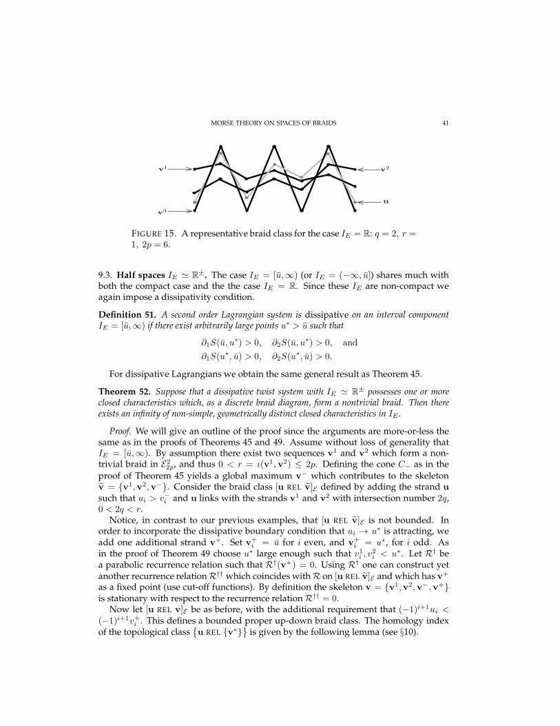
MORSE THEORY ON SPACES OF BRAIDS 41
PSfrag replacements
u
v1v2
v3
FIGURE 15. A representative braid class for the case IE = R: q = 2, r =1, 2p = 6.
9.3. Half spaces IE ≃ R±. The case IE = [u,∞) (or IE = (−∞, u]) shares much withboth the compact case and the the case IE = R. Since these IE are non-compact weagain impose a dissipativity condition.
Definition 51. A second order Lagrangian system is dissipative on an interval componentIE = [u,∞) if there exist arbitrarily large points u∗ > u such that
∂1S(u, u∗) > 0, ∂2S(u, u
∗) > 0, and
∂1S(u∗, u) > 0, ∂2S(u
∗, u) > 0.
For dissipative Lagrangians we obtain the same general result as Theorem 45.
Theorem 52. Suppose that a dissipative twist system with IE ≃ R± possesses one or moreclosed characteristics which, as a discrete braid diagram, form a nontrivial braid. Then thereexists an infinity of non-simple, geometrically distinct closed characteristics in IE .
Proof. We will give an outline of the proof since the arguments are more-or-less thesame as in the proofs of Theorems 45 and 49. Assume without loss of generality thatIE = [u,∞). By assumption there exist two sequences v1 and v2 which form a non-trivial braid in E2
2p, and thus 0 < r = ι(v1,v2) ≤ 2p. Defining the cone C− as in the
proof of Theorem 45 yields a global maximum v− which contributes to the skeletonv = v1,v2,v−. Consider the braid class [u REL v]E defined by adding the strand u
such that ui > v−i and u links with the strands v1 and v2 with intersection number 2q,0 < 2q < r.
Notice, in contrast to our previous examples, that [u REL v]E is not bounded. Inorder to incorporate the dissipative boundary condition that ui → u∗ is attracting, weadd one additional strand v+. Set v+
i = u for i even, and v+i = u∗, for i odd. As
in the proof of Theorem 49 choose u∗ large enough such that v1i , v2i < u∗. Let R† be
a parabolic recurrence relation such that R†(v+) = 0. Using R† one can construct yetanother recurrence relation R†† which coincides with R on [u REL v]E and which has v+
as a fixed point (use cut-off functions). By definition the skeleton v = v1,v2,v−,v+is stationary with respect to the recurrence relation R†† = 0.
Now let [u REL v]E be as before, with the additional requirement that (−1)i+1ui <(−1)i+1v+i . This defines a bounded proper up-down braid class. The homology indexof the topological class
u REL v∗
is given by the following lemma (see §10).

42 R.W. GHRIST, J.B. VAN DEN BERG, AND R.C. VANDERVORST
Lemma 53. The Conley homology of H(u REL v∗) is given by
(52) CHk(H) =
R : k = 2q − 1, 2q0 : else
In particular CPt(H) = t2q−1(1 + t).
For the remainder of the proof we refer to that of Theorem 45.
PSfrag replacements
u
v1v2
v+
v−
FIGURE 16. A representative braid class for the case IE = R±: q =1, r = 4, 2p = 6.
9.4. A general multiplicity result and singular energy levels.
9.4.1. Proof of Theorem 1. Lagrangians for which the above mentioned dissipativity con-ditions are satisfied for all (non-compact) interval components at energy E, are called
dissipative at E.16 For such Lagrangians the results for the three different types of in-terval components are summarized in Theorem 1 in §1. The fact that the presence of anon-simple closed characteristic, when represented as a braid, yields a non-trivial, non-maximally linked braid diagram, allows us to apply all three Theorems 45, 49, and 52,proving Theorem 1.
9.4.2. Singular energy levels. The forcing theorems in §9.1 - §9.3 are applicable for allregular energy levels provided the correct configuration of closed characteristics can befound a priori. In this section we will discuss the role of singular energy levels; theymay create configurations which force the existence of (infinitely) many periodic orbits.The equilibrium points in these singular energy levels act as seeds for the infinite familyof closed characteristics.
For singular energy levels the set UE is the union of several interval components, forwhich at least one interval component contains an equilibrium point. If ∂2uL(u∗, 0, 0) > 0at an equilibrium point u∗, then such a point is called non-degenerate and is contained inthe interior of an interval component. For applying our results of the previous sectionthe nature of the equilibrium points may play a role.
16One class of Lagrangians that is dissipative on all its regular energy levels is described by
limλ→∞
λ−sL(λu, λ2+s4 v, λ
s2 w) = c1|w|2 + c2|u|
s, for some s > 2, and c1, c2 > 0,
pointwise in (u, v, w).

MORSE THEORY ON SPACES OF BRAIDS 43
Γ+
D+
D−
u2 = u∗
2
u1=
u∗ 1
u1=u2
b
b
b
b
u+
u−
(b, b)
(a, a)
D1
u2 = u∗
2
u1=
u∗ 1
u1=u2
b
b
u−
FIGURE 17. The gradient of W2 for the case with two equilibria anddissipative boundary conditions. On the left, for E = 0, the regions D±with the maxima and minima u± are depicted, as well as the superlevelset Γ+. On the right, for E ∈ (0, c0), the region D1, containing an index1 point, is indicated.
9.4.3. Case I: IE = R. We examine the case of a singular energy level E = 0 such thatIE = R and IE contains at least two equilibrium points. One observes that if the equi-libria can be regarded as periodic orbits then Theorem 49 would apply: a regularizationargument makes this rigorous. LetE = 0 be the energy level in which UE is the concate-nation of three interval components (−∞, a]∪[a, b]∪[b,∞), i.e., the equilibria are a and b.We remark that the nature of the equilibrium points is irrelevant; there is a global reasonfor the existence of two unlinked periodic orbit in the energy levels E ∈ (0, c0) for somesmall c0 > 0, see [58]. In these regular energy levels we can apply Theorem 49, anda limit procedure ensures that the periodic solutions persist to the degenerate energylevel E = 0, proving Theorem 2.
Recall from [58] that two equilibrium points imply the existence of maximum u+ andminimum u−, both simple closed characteristics, see Fig. 17. Define the regions D+ =(u1, u2) |u2 − u1 > 0, u1 ≥ a, u2 ≤ b, and D− = (u1, u2) |u∗1 ≤ u1 ≤ a, b ≤ u2 ≤ u∗2,where (u∗1, u
∗2) is the point where the dissipativity condition of Definition 48 is satisfied.
Then u+ ∈ D+ and u− ∈ D−.SinceW2 is aC2-function on int(D+) it follows from Sard’s theorem that there exists a
regular value e+ such that 0 ≤ max∂D+W2 < e+ < maxD+
W2. Consider the connectedcomponent of the super-level set W2 ≥ e+ which contains u+. The outer boundary ofthis component is a smooth circle and ∇W2 points inwards on this boundary circle. LetΓ+ be the interior of the outer boundary circle in question. By continuity it follows thatthere exists a positive constant c0 such that Γ+ remains an isolating neighborhood forE ∈ (0, c0). In the following let E ∈ (0, c0) be arbitrary.
Define D1 = (u1, u2) |u2 − u1 ≥ ǫ, u−1 ≤ u1 ≤ u+1 , u2 ≤ u+2 ∪ Γ+. It follows fromthe properties of S (see §8) that D1 is again an isolating neighborhood, see Fig. 17. It

44 R.W. GHRIST, J.B. VAN DEN BERG, AND R.C. VANDERVORST
holds that CPt(D1) = 0, and D1\Γ+,Γ+ forms a Morse decomposition. The Morserelations (39) yield
CPt(Γ+) + CPt(D1\Γ+) = 1 + CPt(D1\Γ+) = (1 + t)Qt,
where Qt is a nonnegative polynomial. This implies that D1\Γ+ contains an index 1solution u1. We can now define D2 = (u1, u2) |u2 − u1 ≥ ǫ, u+1 ≤ u1, u
+2 ≤ u2 ≤
u−2 ∪ Γ+. In exactly the same way we find an index 1 solution u2 ∈ D2. Notice, that byconstruction ι(u1,u2) = 0. Theorem 49 now yields an infinity of closed characteristicsfor all 0 < E < c0. As described in §9.2 these periodic solutions can be characterizedby p and q, where (p, q) is any pair of integers such that q < p and p and q are relativeprime (or p = q = 1). Here 2p is the period of the solution up,q and 2q = ι(up,q ,u
1) =ι(up,q ,u
2).In the limit E → 0 the solutions u1 and u2 may collapse onto the two equilibrium
points (if they are centers). Nevertheless, the infinite family of solutions still exists inthe limit E = 0, because the extrema of the associated closed characteristics may onlycoalesce in pairs at the equilibrium points. This follows from the uniqueness of theinitial value problem of the Hamiltonian system. Hence in the limit E → 0 the type(p, q) of the periodic solution is conserved when we count extrema with multiplicity andintersections without multiplicity.
Note that when the equilibria are saddle-foci then u1 and u2 stay away from ±1 inthe limit E → 0. Extrema may still coalesce at the equilibrium points as E → 0, butintersections are counted with respect to u1 and u2. Finally, in the regular energy levelsE ∈ (0, c0), Theorem 49 provides at least two solutions of each type (except p = q = 1);in the limit E = 0 one cannot exclude the possibility that two solutions of the same typecoincide.
Remark 54. Theorem 2, proved in this subsection, is immediately applicable to theSwift-Hohenberg model (3) as described in §1. Notice that if the parameter α satisifiesα > 1, then Theorem 2 yields the existence of infinitely many closed chararacteristics
at energy E = − (α−1)2
4 , and nearby levels. However from the physical point of view itis also of interest to consider the case α ≤ 1. In that case there exists only one singularenergy level and one equilibrium point. This case can be treated with our theory, but thenature of the equilibrium point comes into play. If an equilibrium point is a saddle orsaddle-focus, it is possible that no additional periodic orbits exist (see [57]). However, ifthe equilibrium point is a center an initial non-simple closed characteristic can be foundby analyzing an improper braid class, which by, Theorem 1, then yields infinitely manyclosed characteristics. The techniques involved are very similar to those used in thepresent and subsequent sections. We do not present the details here as this falls outsideof the scope of this paper.
9.4.4. Cases II and III: IE = [a, b] or IE = R±. The remaining cases are dealt with inTheorem 3. We will restrict the proof here to the case that IE contains an equilibrium
point that is a saddle-focus — the center case can be treated as in [2].17 It also follows
17Indeed, for energy levels E+ c, c sufficiently small, a small simple closed charecteristic exists due to thecenter nature of the equilibrium point at E; spectrum ±ai,±bi, a < b. This small simple closed character-istic will have a non-trivial rotation number close to a
b. The fact that the rotation number is non-zero allows

MORSE THEORY ON SPACES OF BRAIDS 45
for the previous that there is no real difference between IE being compact or a half-line.For simplicity we consider the case that IE is compact.
D
u2 = b
u1=a
u 1=u 2
b(u∗ , u
∗ )
FIGURE 18. [left] The gradient of W2 for the case of one saddle-focusequilibrium and compact boundary conditions. Clearly a saddle pointis found inD. [right] The perturbation of one equilibrium to three equi-libria.
Let us first make some preliminary observations. When u∗ is a saddle-focus, then inE = 0 there exists a solution u1 such that u11 < u∗ < u12. This follows from the fact thatthere is a point (u∗1, u
∗2), u
∗1 < u∗2, close to (u∗, u∗) at which the vector ∇W2 points to the
north-west (see Fig. 18 and [58]). This solution u1 is a saddle point, its rotation numberbeing unknown. The impression is that (u∗, u∗) is a minimum (with τ = 0), and if u∗were a periodic solution, then one would have a linked pair (u∗, u∗) and u1 to whichone could apply Theorem 45. Since u∗ is a saddle-focus it does not perturb to a periodicsolution for E > 0. Hence we need to use a different regularization which conveys theinformation that u∗ acts as a minimum. The form of the perturbation that we have inmind is depicted in Fig. 18, where we have drawn the “potential” L(u, 0, 0).
This idea can be formalized as follows. Choose a function T ∈ C∞0 [0,∞) such that
0 ≤ T (s) ≤ 1, T (s) = 1 for x ≤ 12 , T (s) strictly decreases on (12 , 1) and T (s) = 0 for
x ≥ 1. Add a perturbation
Φǫ(u) =
∫ u
u∗
−2C0 (s− u∗)T( |s− u∗|
ǫ
)ds
to the Lagrangian, i.e. L = L+Φǫ(u), whereC0 = ∂2uL(u∗, 0, 0). The new Euler-Lagrangeequation near u∗ becomes
∂2uxxLuxxxx +
[2∂2uxxuL− ∂2ux
L]uxx + ∂2uL
[1− 2T
( |u−u∗|ǫ
)](u − u∗) = O(U2),
where all partial derivatives of L are evaluated at (u∗, 0, 0), and where U is the vector(u−u∗, ux, uxx, uxxx) in phase space. Hence for all small ǫ there are now two additionalequilibria near u∗, denoted by u ∈ (u∗ − ǫ, u∗ − ǫ/2) and u ∈ (u∗ + ǫ/2, u∗ + ǫ). Since
one to use the arguments in [2] to construct a non-simple closed characteristic. As a matter of fact a linked
braid diagram is created this way.

46 R.W. GHRIST, J.B. VAN DEN BERG, AND R.C. VANDERVORST
(u∗ − u)− (u− u∗) = O(ǫ2), the difference between E(u) and E(u) is O(ǫ2). To level this
difference we add another small perturbation to L of the form Ψ(u) =∫ u
u∗
CǫT (|s−u∗|
2ǫ )ds,
i.e. L(u) = L(u) + Ψ(u), where Cǫ is chosen so that E(u) = E(u) (of course uand u shift slightly), and Cǫ = O(ǫ2). Using the same analysis as before we con-clude that a neighborhood of u∗ in the energy level E(u) looks just like Fig. 17. InB = (u1, u2) |u∗1 < u1 < u, u < u2 < u∗2 we find a minimum. Choose an regular en-
ergy levelEǫ slightly larger than E(u) = E(u) (withEǫ = O(ǫ)), such that the minimumin B persists. Taking this minimum and the original u1 — which persists since we haveonly used small perturbations, preserving D (see Fig. 18) as an isolating neighborhood— we apply Theorem 45.
Finally, we take the limit ǫ → 0. The solutions now converge to solutions of theoriginal equation in the degenerate energy level. It follows that in the energy levelE = 0 a solution of type (p, q) exists, where the number of extrema has to be countedwith multiplicity since extrema can coalesce in pairs at u∗.
10. COMPUTATION OF THE HOMOTOPY INDEX
Theorems 45, 49, and 52 hang on the homology computations of the homotopy in-variant for certain canonical braid classes (Lemmas 47, 50, and 53). Our strategy (as in,e.g., [2]) is to choose a sufficiently simple system (an integrable Hamiltonian system)which exhibits the braids in question and to compute the homotopy index via knowingthe structure of an unstable manifold. By the topological invariance of the homotopyindex, any computable case suffices to give the index for any period d.
Consider the first-order Lagrangian system given by the Lagrangian Lλ(u, ux) =12 |ux|2 + λF (u), where we choose F (u) to be an even four-well potential, with F ′′(u) ≥−1, and F ′′(0) = −1. The Lagrangian system (Lλ, dx) defines an integrable Hamiltoniansystem on R2, with phase portrait given in Fig. 19.
FIGURE 19. The integrable model in the (u, ux) plane; there are centersat 0,±2 and saddles at ±1,±3.
Linearization about bounded solutions u(x) of the above Lagrangian system yieldsthe quadratic form
Q[φ] =
∫ 1
0
|φx|2dt+ λ
∫ 1
0
F ′′(u(x))φ2dx ≥∫ 1
0
(π2 − λ)φ2dx, φ ∈ H10 (0, 1),

MORSE THEORY ON SPACES OF BRAIDS 47
which is strictly positive for all 0 < λ < π2. For such choices of λ the time-1 mapdefined via the induced Hamiltonian flow ψx, i.e., (u, pu) = (u, ux) 7→ ψ1(u, pu), is anarea preserving monotone twist map. The generating function of the twist map is givenby the minimization problem
Sλ(u1, u2) = infq∈X(u1,u2)
∫ 1
0
Lλ(u, ux)dx,
where X(u1, u2) = u ∈ H1(0, 1) | u(0) = u1, u(1) = u2.18 The function Sλ is asmooth function on R2, with ∂1∂2Sλ > 0. The recurrence function Rλ(ui−1, ui, ui+1) =∂2Sλ(ui−1, ui) + ∂1Sλ(ui, ui+1) satisfies Axioms (A1)-(A3), and thus defines an exact(autonomous) parabolic recurrence relation on X = RZ. We choose the potential F suchthat the bounded solutions within the heteroclinic loop between u = −1 and u = +1have the property that the period Tλ is an increasing function of the amplitude A, andTλ(A) → 2π√
λ, as A→ 0.
This single integrable system is enough to compute the homotopy index of the threefamilies of braid classes in Lemmas 47, 50, and 53 in §9.
We begin by identifying the following periodic solutions. Set v1,± = v1,±i , v1,±i =
±3, and v2,± = v2,±i , v2,±i = ±1. Let u(t) be a solution of (Lλ, dx) with ux(0) = 0(minimum), |u(x)| < 1, and T1(A(u)) = 2τ0 > 2π, τ0 ∈ N. For arbitrary λ ≤ 1 thisimplies that
Tλ(A(u)) =T1(A(u))√
λ=
2τ0√λ,
where we choose λ so that 1√λ∈ N. For r ≥ 1 set d := τ0r√
λand define v3 := v3i , with
v3i = u(i), and v4 = v4i , with v4i = u(i + τ0/√λ), i = 0, ..., d. Clearly, ι(v3,v4) = r, for
all 1√λ∈ N.
Next choose u(x), a solution of (Lλ, dx) with ux(0) = 0 (minimum), which oscil-lates around both equilibria −2 and +2, and in between the equilibria −3 and +3, andT1(A(u)) = 2τ1 > 2π, τ1 ∈ N. As before
Tλ(A(u)) =T1(A(u))√
λ=
2τ1√λ.
Let 2p ≥ r and choose τ0, τ1 ≥ 4 such that
τ0τ1
=2p
r≥ 1 (τ0 ≥ τ1).
Set v5 = v5i , v5i = u(i), and v6 = v6i , with v6i = u(i + τ1/√λ), i = 0, ..., d. For
x ∈ [0, d] the solutions u and u have exactly 2p intersections. Therefore, if we choose λsufficiently small, i.e. 1√
λ∈ N is large, then it also holds that ι(v3,4,v5,6) = 2p.
Finally we choose the unique periodic solution u(x), with |u(x)| < 1, ux(0) = 0(minimum), and T1(A(u)) = 2τ2 > 2π, τ2 ∈ N. Let 0 < 2q < r ≤ 2p, and choose τ2, andconsequently the amplitude A, so that
τ0τ2
=2q
r< 1 (τ0 < τ2, A(u)) < A(u)).
18 The strict positivity of the quadratic form Q via the choice of λ yields a smooth family of hyperbolic
minimizers.

48 R.W. GHRIST, J.B. VAN DEN BERG, AND R.C. VANDERVORST
The solution u is part of a hyperbolic circle of solutions us(x), s ∈ R/Z. Define
(u(s))s∈R/Z, with u(s) = ui(s), where ui(s) = us(i + 2τ2s/√λ). As before, since
the intersection number of u and us is equal to 2q, it holds that ι(u(s),v3,4) = 2q, for λsufficiently small. Moreover, ι(u(s),v5,6) = 2p. From this point on λ is fixed. We nowconsider three different skeleta v.
I: v = v2,−,v2,+,v3,v4. The relative braid class [u REL v]I is defined as follows:
v2,−i ≤ ui ≤ v2,+i , and u links with the strands v3 and v4 with intersection number 2q,0 ≤ 2q < r. The topological class
u REL v
is precisely that of Lemma 47 [Fig. 14]
and as such is bounded and proper.II: v = v2,−,v1,+,v3,v4,v5. The relative braid class [u REL v]II is defined as fol-
lows: v2,−i ≤ ui ≤ v1,+i , u links with the strands v3 and v4 with intersection number2q, 0 ≤ 2q < r, and u links with v5 with intersection number 2p. The topological classu REL v
is precisely that of Lemma 53 [Fig. 16] and as such is bounded and proper.
III: v = v2,−,v3,v4,v5,v6. The relative braid class [u REL v]III is defined as fol-
lows: v2,−i ≤ ui, u links with the strands v3 and v4 with intersection number 2q, and u
links with v5 and v6 with intersection number 2p. The topological classu REL v
is
not bounded [Fig. 20[right]]. The augmentation of this braid class is bounded.
Cases I and II: Since the topological classes are bounded and proper, the invariant H isindependent of period of the chosen representative, and can be easily computed fromthe integrable model. The closure of the collection of topologically equivalent braidclasses is an isolating neighborhood for the parabolic flow Ψt induced by the recur-rence relation Rλ = 0 (defined via (Lλ, dx)). The invariant set is given by the normallyhyperbolic circle u(s)s∈R/Z. For this reason the index H can be computed via theconnected component that contains the critical circle; we denote this neighborhood byN . The Conley index of N can be determined via computing Wu(u(s)), the unstablemanifold associated to this circle. This computation is precisely that appearing in thecalculations of [2, pp. 372]: Wu(u(s)) is orientable and of dimension 2q, and thus
(53) H(u REL v) = h(N) ≃(S1 × S2q−1
)/(S1 × pt
)≃ S2q−1 ∨ S2q.
The Conley homology is given by CHk(H) = R for k = 2q − 1, 2q, and CHk(H) = 0elsewhere. This completes the proofs of the Lemmas 47 and 53.
Case III: It holds that u REL v
∩(D1
2p REL v)6= ∅.
The discrete class for period 2p is bounded, but for periods d > 2p this is not the case.However, by augmenting the braid, we obtain from (27) that
H(u REL v) = H(u REL v∗),
where v∗ = v ∪ v1,−,v1,+. Since the topological classu REL v∗
is bounded and
proper, we may use the previous calculations to conclude that
H(u REL v∗) ≃ (S1 × S2q−1)/(S1 × pt) ≃ S2q−1 ∨ S2q.
Our motivation for this computation is to complete the proof of Lemma 50. Let[u′ REL v′] denote the period 2p braid class described by Fig. 15, with intersection num-bers denoted by 2q′ and 2r′, and let [u REL v] denote a type-III braid of period 2p. Then,

MORSE THEORY ON SPACES OF BRAIDS 49
PSfrag replacements
D
FIGURE 20. The augmentation of the braid from Lemma 50 [left] is thedual of the type III braid [right].
it is straightforward to see (as illustrated in Fig. 20) that, for q′ = p− q and r′ = 2p− r,
(54)[u′
REL [v′ ∗]]= D
([u REL [v]
]).
Lemma 50 gives the index for the augmented classu′ REL v′ ∗
, which is bounded
and proper as a topological class. The above considerations allow us to compute thehomology of H(u′ REL v′ ∗) via Theorem 30:
(55)
CH∗(H(u′ REL v′ ∗)
) ∼= CH∗ (H(Du REL Dv))∼= CH2p−∗ (H(u REL v))∼= CH2p−∗ (H(u REL v∗))
∼=R : 2p− ∗ = 2q − 1, 2q0 : else
∼=R : ∗ = 2q′, 2q′ + 10 : else
.
The intersection numbers 2q′ and 2r′ are exactly those of Lemma 50, completing theproof.
11. POSTLUDE
11.1. Extensions and questions: dynamics. There are several ways in which the basicmachinery introduced in this paper can be generalized to other dynamical systems.1. Scalar uniformly parabolic PDEs. Theorem 19 suggests strongly that the homotopyindex for discretized braids extends to and agrees with an analogous index for parabolicdynamics on spaces of smooth curves via uniformly parabolic PDE’s. This is true [23].2. Periodicity in the range. Although we consider the anchor points to be in R, one mayjust as well constrain the anchor points to lie in S1 and work in the universal cover. Suchadditional structure is used in the theory of annulus twist maps [2, 7, 36, 37, 42]. All ofour results immediately carry over to this setting. We note that compact-type boundaryconditions necessarily follow.
3. Aperiodic dynamics. One can also extend the theory to include braid diagrams with“infinite length” strands. To be more precise, consider braid diagrams on the infinite 1-dlattice, and omit the spatial periodicity. In this context several compactness issue comeinto play. To name a few: (a) the parabolic flows generated by aperiodic recurrence

50 R.W. GHRIST, J.B. VAN DEN BERG, AND R.C. VANDERVORST
relations no longer live on a finite dimensional space but on the infinite dimensionalspace ℓ∞(R). See [2] for a case similar to this; (b) a priori, the Conley index should bereplaced with an infinite dimensional analogue such as that developed by Rybakowski[52]. However, if one considers braid diagrams with finite word metric, the stabilizationtheory of §5 allows one to define the necessary invariants via the finite dimensionaltheory in this paper. This is not unlike the procedure one can follow in the treatment ofparabolic PDE’s [23].
4. Fixed boundary conditions. Our decision to use closed braid diagrams is motivatedby applications in Lagrangian systems; however, one can also fix the end points of thebraid diagrams. In this setting one can define a braid invariant in the same spirit as isdone for closed braids. The proof of stabilization is not sensitive to the type of boundaryconditions used. Such an extension of the theory to include fixed endpoints is useful inapplications to parabolic PDE’s [23].
5. Traveling waves and period orbits. The stationary solutions we find in this paper arebut the beginnings of a dynamical skeleton for the systems considered. The next logicalstep would be to classify connecting orbits between stationary solutions: several authors(e.g., [40]) have considered these problems analytically in the context of traveling wavephenomena in monotone lattice dynamics. There is a precedent of using Conley indicesto prove existence theorems for connecting orbits (e.g., [47]): we anticipate that suchapplications are possible in our setting. One could as well allow the skeletal strands tobe part of a periodic motion (in the case of non-exact recurrence relations). In this settingone could look for both fixed points and periodic solutions of a given braid class.
6. Long-range coupling. Assume that the recurrence relations Ri are functions of the formRi(ui−n, . . . , ui+n) for some n. Even if a strong monotonicity condition holds, ∂jRi > 0for all j 6= i the proof of Proposition 11 still encounters a difficulty: two strands witha simple (codimension-one) tangency can have enough local crossings to negate theparabolic systems’ separation. Such monotone systems do exhibit an ordering principle[3, 26] (initially nonintersecting strands will never intersect), but additional braidingphenomena is not automatically present.
7. Higher-dimensional lattice dynamics. In parabolic PDE’s of spatial dimension greaterthan one, the straightforward generalization of the lap number (number of connectedcomponents of an intersection of graphs) does not obey a monotonicity property (due tothe fact that for graphs of Rn with n > 1, critical points of non-zero index and co-indexcan pass through each other). Finding a suitable form of dynamics which retains someisolation remains an important and challenging problem.
8. Arbitrary second-order Lagrangians. Our principal dynamical goal is to prove exis-tence theorems for periodic orbits with a minimal amount of assumptions, particularly“genericity” assumptions (which are, in practice, rarely verifiable). To this end, we havebeen successful for second-order Lagrangians modulo the twist assumption. Althoughthis assumption is provably satisfied in numerous contexts, we believe that it is not,strictly speaking, necessary. Its principal utility is in the reduction of the problem to afinite-dimensional recurrence relation. We believe that the forcing results proved in §8are valid for all second-order Lagrangian systems. See for instance [31] for a result onthat behalf. We propose that a version of the curve-shortening techniques in the spirit

MORSE THEORY ON SPACES OF BRAIDS 51
of Angenent [4] should yield a homotopy index for smooth curves to which our forcingtheorems apply.
11.2. Extensions and questions: topology. The homotopy index is, as a topological in-variant of braid pairs, utterly useless. Nevertheless, there is topological meaning intrin-sic to this index, the precise topological interpretation of which is as yet unclear. Oneobserves that the index captures some Morse-theoretic data about braid classes. Anytopological interpretation is certainly related to linking data of the free strands with theskeleton, as evidenced by the examples in this paper. Though the total amount of link-ing should provide some upper bound to the dimension of the homotopy index, linkingnumbers alone are insufficient to characterize the homotopy index.
We close with several related questions about the homotopy index itself.
1. Realization. It is clear that given any polynomial in t, there exists a braid pair whosehomological Poincare polynomial agrees with this. [Idea: take Example 3 of §4 andstack disjoint copies of the skeleton vertically, using as many free copies and strands asnecessary to obtain the desired homology.] Can a realization theorem be proved for thehomotopy index itself? As a first step to this, consider replacing the real coefficients inthe homological index with integral coefficients. Does torsion ever occur? We believenot, with the possible exception of a Z2 torsion.
2. Product formulas and the braid group. Perhaps the most pressing problem for the homo-topy index is to determine a product formula for the concatenation of two braids withcompatible skeleta. This would eliminate the need for computing the index via contin-uation to an integrable model system as in §10. However, since we work on spaces ofclosed braids, a product formula is not well-defined. The group structure on the braidgroup Bn does not extend naturally to a group structure on conjugacy classes: whereone “cuts open” the braid to effect a gluing can change the resulting braid class dramat-ically. The one instance in which a product operation is natural is a power of a closedbraid. Here, splitting the closed braid to an open braid and concatenating several copiesthen reclosing yields equivalent closed braids independent of the representative of theconjugacy class chosen. Such a product/power formula, in conjunction with numericalmethods of index computation effective in moderately low dimensions, would allowone to compute many invariants.
3. Improper and unbounded classes In certain applications one also needs to deal withimproper braid classes [u REL v]. To such classes one can also assign an index. Theinterpretation of the index as a Morse theory will not only depend on the topologicaldata, but also on the behavior of the flow Ψt at Σ−. The simplest case is when Σ− ∩ ∂Nconsists of finitely many points. This for example happens when u consists of only onestrand. The homotopy index is then defined by the intrinsic definition in (15). The in-terpretation of the index and the associated Morse theory depends on the linearizationDΨt|Σ−∩∂N . The definition of the index in the case of more complicated sets Σ− ∩ ∂Nand the Morse theoretic interpretation will be subject of future study. Similar consider-ations hold for unbounded classes.
4. General braids. The types of braids considered in this paper are positive braids. Natu-rally, one wishes to extend the ideas to all braids; however, several complications arise.

52 R.W. GHRIST, J.B. VAN DEN BERG, AND R.C. VANDERVORST
First, passing to discretized braids is invalid — knowing the anchor points is insuf-ficient data for reconstructing the braid. Second, compactness is troublesome — onecannot merely bound braid classes via augmentation. We can model general braidsdynamically using recurrence relations with nearest neighbor coupling allowing “pos-itive”, or “negative” interaction. This idea appears in the work of LeCalvez [36, 37]and can be translated to our setting via a change of variables — coordinate flips — ofwhich our duality operator D is a particular example. However the compactness anddiscretization issues remain. LeCalvez works in the setting of annulus maps, where onecan circumvent these problems: the general setting is more problematic.
5. Hamiltonian vs. Lagrangian. One approach to extending to arbitrary braids would beto switch from a Lagrangian setting to a Hamiltonian setting. Consider an S1 familyof Hamiltonians Ht on a symplectic surface (M2, ω) which has a “skeleton” of periodicorbits braided in M ×S1. Adding “free” braid strands, one could define a relative Floerindex for the system which should detect whether the free strands are forced to exist asperiodic orbits.
REFERENCES
[1] N.N. Akmediev, A.V. Buryak and M. Karlsson, Radiationless optical solitons with oscillating tails, Opt. Comm.110 (1994), 540-544.
[2] S.B. Angenent, The periodic orbits of an area preserving Twist-map, Comm. Math. Phys. 115 (1988), 353-374.[3] S.B. Angenent, Monotone recurrence relations, their Birkhoff orbits and topological entropy, Erg. Th. & Dyn. Syst.
10 (1990), 15-41.[4] S.B. Angenent, Curve Shortening and the topology of closed geodesics on surfaces, preprint 2000.[5] S.B. Angenent, The zero set of a solution of a parabolic equation, J. Reine Angew. Math. 390 (1988), 79-96.[6] S.B. Angenent, J.B. Van den Berg and R.C. Vandervorst, Contact and noncontact energy hypersurfaces in second
order Lagrangian systems, preprint 2001.[7] S. Aubry and P.Y. LeDaeron, The Frenkel-Kontorova model and its extensions, Physica D, 8 (1983), 381-422.[8] J. Birman, Braids, links and the mapping class group, Annals of Mathematics Studies vol. 82, Princeton Press,
(1975).[9] P. Boyland, Topological methods in surface dynamics, Topology & its Applications 58:3, (1994), 223–298.[10] P. Brunovsky and B. Fiedler, Connecting orbits in scalar reaction-diffusion equations. Dynamics Reported 1,
(1988), 57-89.[11] C. Conley, Isolated invariant sets and the Morse index, C.B.M.S. Reg. Conf. Ser. Math. 38 (1978), published
by the AMS.[12] C. Conley and P. Fife, Critical manifolds, travelling waves, and an example from population genetics, J. Math.
Biol. 14 (1982), 159-176.[13] C. Conley and E. Zehnder, The Birkhof-Lewis fixed point theorem and a conjecture of V.I. Arnol’d, Invent. Math.
73 (1983), 33-49.[14] C. Conley and E. Zehnder, Morse-type index theory for flows and periodic solutions for Hamiltonian equations,
Comm. Pure Appl. Math. 37(2) (1984), 207-253.[15] N. Dancer, Degenerate critical points, homotopy indices and Morse inequalities, J. Reine Angew. Math. 350
(1984), 1-22.[16] Y. Eliashberg, A. Givental, and H. Hofer. An introduction to symplectic field theory. Geom. Func. Anal.,
Special Volume II (2000), 560-673.[17] A. Floer, A refinement of the Conley index and an application to the stability of hyperbolic invariant sets, Ergod.
Th. & Dynam. Sys. 7 (1987), 93-103.[18] B. Fiedler and J. Mallet-Paret, A Poincare-Bendixson theorem for scalar reaction diffusion equations, Arch. Rat.
Mech. 107 (1989), 325-345.[19] B. Fiedler and C. Rocha, Realization of meander permutations by boundary value problems, J. Differential
Equations, 156:2 (1999), 282–308.

MORSE THEORY ON SPACES OF BRAIDS 53
[20] B. Fiedler and C. Rocha, Orbit equivalence of global attractors of semilinear parabolic differential equations,Trans. Amer. Math. Soc. 352(1) (2000), 257-284.
[21] G. Fusco and W.M. Oliva, Transversality between invariant manifolds of periodic orbits for a class of monotonedynamical systems, J. Dyn. Diff. Eqns. 2 (1990), 1-17.
[22] G. Fusco and W. Oliva, Jacobi matrices and transversality, Proc. Roy. Soc. Edinburgh Sect. A, 109:3-4, (1988),231–243.
[23] R. Ghrist, and R.C. Vandervorst, Scalar parabolic dynamics via braids, in progress.[24] R. Ghrist and R.C. Vandervorst, Braids and scalar parabolic PDEs, in Proceedings of New Directions in
Dynamics Systems: Kyoto 2002.[25] V. L. Hansen, Braids and Coverings: Selected Topics, Cambridge University Press, 1989.[26] M. Hirsch, Systems of differential equations which are competitive or cooperative, I: Limit sets, Siam J. Math.
Anal. 13 (1982), 167-179.[27] H. Hofer, Pseudo-holomorphic curves and the Weinstein conjecture in dimension three, Invent. Math. 114 (1993),
515-563.[28] H. Hofer and E. Zehnder, Symplectic invariants and Hamiltonian dynamics, Birkhauser, 1993.[29] J. Hulshof, J.B. Van den Berg and R.C.A.M. Vandervorst, Traveling waves for fourth-order semilinear parabolic
equations, Siam J. Math. Anal. 32(6) (2001), 1342-1374.[30] W.D. Kalies and P.J. Holmes, On a dynamical model for phase transformation in nonlinear elasticity, Pattern
formation: symmetry methods and applications (Waterloo, ON, 1993), 255-269, Fields Inst. Commun., 5,Amer. Math. Soc., Providence, RI, 1996.
[31] W.D. Kalies and R.C.A.M. Vandervorst, Closed characteristics of second order Lagrangians, preprint 2002.[32] W.D. Kalies, J. Kwapisz and R.C.A.M. Vandervorst, Homotopy classes for stable connections between Hamil-
tonian saddle-focus equilibria, Comm. Math. Phys. 193 (1998), 337-371.[33] W.D. Kalies, J. Kwapisz, J.B. Van den Berg and R.C.A.M. Vandervorst, Homotopy classes for stable periodic
and chaotic patterns in fourth-order Hamiltonian systems, Comm. Math. Phys. 214(3) (2000), 573-592.[34] J. Kwapisz, Uniqueness of the stationary wave for the extended Fisher-Kolmogorov equation, preprint (1997), J.
Diff. Eqns. 165(1) (2000), 235-253.[35] J. Kwapisz, personal communication.[36] P. LeCalvez, Propriete dynamique des diffeomorphismes de l’anneau et du tore, Asterique 204, 1991.[37] P. LeCalvez, Decomposition des diffeomorphismes du tore en applications deviant la verticale, Mem. Soc. Math.
Fr. (N.S.), No. 79, (1999).[38] A. Leizarowitz and V.J. Mizel, One-dimensional infinite-horizon variational problems arising in continuum
mechanics, Arch. Rat. Mech. Anal. 106(2) (1989), 161-194.[39] J. Mallet-Paret and H.L. Smith, The Poincare-Bendixson theorem for monotone cyclic feedback systems, J. Dyn.
Diff. Eqns. 2 (1990), 367-421.[40] J. Mallet-Paret, The global structure of traveling waves in spatially discrete dynamical systems, J. Dynam. Dif-
ferential Equations, 11:1, (1999), 49–127.[41] H. Matano, Nonincrease of the lap-number of a solution for a one dimensional semilinear parabolic equation, J.
Fac.Sci. Univ. Tokyo 29 (1982), 401-441.[42] J.N. Mather, Existence of quasi-periodic orbits for twist diffeomorphisms of the annulus, Topology 21 (1982),
457-467.[43] J.N. Mather, Amount of rotation about a point and the morse index, Comm. Math. Phys. 94 (1984), 141-153.[44] C. McCord, Poincare-Lefschetz duality for the homology Conley index, Trans. Amer. Math. Soc., 329:1 (1992),
233-252.[45] A. Middleton, Asymptotic uniqueness of the sliding state for charge-density waves, Phys. Rev. Lett. 68:5 (1992),
670-673.[46] J. Milnor, Morse Theory. Annals of Mathematics Studies vol. 51, Princeton Press, 1963.[47] K. Mischaikow, Recent developments in Conley index theory, Springer Lecture Notes in Mathematics vol.
1609, 1995.[48] J. Moser, Monotone twist mappings and the calculus of variations, Erg. Theory Dynam. Systems 6(3) (1986),
401-413.[49] L.A. Peletier and W.C. Troy, Higher order patterns: higher order models in physics and mechanics, Birkhauser,
2001.[50] L.A. Peletier and W.C. Troy, Multibump periodic traveling waves in suspension bridges, Proc. Roy. Soc. Edin.
128A (1998), 631-659.
54 R.W. GHRIST, J.B. VAN DEN BERG, AND R.C. VANDERVORST
[51] L.A. Peletier, W.C. Troy and J.B. Van den Berg Global branches of multi bump periodic solutions of the Swift-Hohenberg equation, Arch. Rat. Mech. Anal. 158 (2001), 91-153.
[52] K. Rybakowski, The homotopy index and partial differential equations, Universitext. Springer-Verlag, Berlin,1987.
[53] J. Smillie, Competitive and cooperative tridiagonal systems of differential equations, Siam J. Math. Anal. 15
(1984), 531-534.[54] C. Sturm, Memoire sur une classe d’equations a differences partielles, J. Math. Pure et Appl. 1 (1836), 373-444.[55] L. Truskinovsky and G. Zanzotto, Ericksen’s bar revisited: energy wiggles, J. Mech. Phys. Solids 44(8) (1996),
1371-1408.[56] P. Van Moerbeke, The spectrum of Jacobi matrices, Invent. Math. 37 (1976), 45-81.[57] J.B. Van den Berg, The phase-plane picture for a class of fourth-order conservative differential equations, preprint
(1998), J. Diff. Eqns. 161(1) (2000), 110-153.[58] J.B. Van den Berg and R.C.A.M. Vandervorst, Fourth order conservative Twist systems: simple closed charac-
teristics, Trans. Amer. Math. Soc. Transactions AMS 354 (2002), 1383-1420.[59] V. Vassiliev, Complements of discriminants of smooth maps: topology and applications, Translated from the
Russian by B. Goldfarb, Amer. Math. Soc., Providence, RI, 1992.[60] F.W. Wilson and J.A. Yorke, Lyapunov functions and isolating blocks, J. Diff. Eqns. 13 (1973), 106-123.
APPENDIX A. CONSTRUCTION OF PARABOLIC FLOWS
In this appendix, we construct particular parabolic flows on braid diagrams in orderto carry out the continuation arguments for the well-definedness of the Conley index forproper braid diagrams. The constructions are explicit and are generated by recurrencerelations R = (Ri)i∈Z, with Ri+d = Ri, which are of the form:
Ri(r, s, t) = ai(r, s) + bi(s, t) + ci(s), i = 1, ..., d,(56)
with ai, bi, ci ∈ C1(R), and ∂ai
∂r (r, s) > 0, ∂bi∂t (s, t) ≥ 0 for all (r, s, t) ∈ R3. By definition,
such recurrence relations are parabolic.
Lemma 55. For any v ∈ Dmd there exists a parabolic flow Ψt under which v is stationary.
Proof. In order to have Ψt(v) = v, the sequences vα need to satisfyRi(v
αi−1, v
αi , v
αi+1) = 0, for some parabolic recurrence relation. We will construct R by
specifying the appropriate functions ai, bi, ci as above. In the construction to follow,the reader should think of the anchor points vαi of the fixed braid v as constants.
For each i such that the values vαi α are distinct, one may choose ai(r, s) = r,bi(s, t) = t, and ci(s) to be any C1 function which interpolates the defined values
ci(vαi ) := −(vαi−1 + vαi+1).
This generates the desired parabolic flow.In the case where there are several strands α1, α2, . . . αn for which v
αj
i = v∗ are allequal, the former construction is invalid: ci is not well-defined. According to Defini-tion 4, we have for each αj 6= αk (v
αj
i−1 − vαk
i−1)(vαj
i+1 − vαk
i+1) < 0. This implies that ifwe order the αjj so that vα1
i−1 < vα2
i−1 < · · · < vαn
i−1, then the corresponding sequence
vαj
i+1j satisfies vαn
i+1 < vαn−1
i+1 < · · · < vα1
i+1. From Lemma 56 below, there exist increas-ing functions f and g such that
f(vαj
i−1)− f(vαk
i−1) = g(vαk
i+1)− g(vαj
i+1) ∀j, k.Define ai and bi in the following manner: set ai(r, v
∗) := f(r) and bi(v∗, t) := g(t). Thus
it follows that there exists a well defined value
ci(v∗) := −
(f(v
αj
i−1) + g(vαj
i+1))

MORSE THEORY ON SPACES OF BRAIDS 55
which is independent of j. For any other strands α′, repeat the procedure, defining
the slices ai(r, vα′
i ), bi(vα′
i , t) and the points ci(vα′
i ), choosing new functions f and gif necessary. To extend these functions to global functions ai(r, s) and bi(s, t), sim-ply perform a C1 homotopy in s without changing the monotonicity in the r and t
variables: e.g., on the interval [vαi , vα′
i ], choose a monotonic function ξ(s) for which
ξ(vαi ) = ξ′(vαi ) = ξ′(vα′
i ) = 0 and ξ(vα′
i ) = 1. Then set
ai(r, s) := (1− ξ(s))ai(r, vαi ) + ξ(s)ai(r, v
α′
i ).
Such a procedure, performed on the appropriate s-intervals, yields a smooth r-monotonic interpolation. Repeat with bi(s, t). Finally, choose any function ci(s) whichsmoothly interpolates the preassigned values. These choices of ai, bi and ci give thedesired recurrence relation, and consequently the parabolic flow Ψt.
Lemma 56. Given two sequences of increasing real numbers x1 < x2 < · · · < xn and y1 <y2 < · · · < yn, there exist a pair of strictly increasing functions f and g such that
(57) f(xj)− f(xk) = g(yj)− g(yk) ∀j, kProof. Induct on n, noting the triviality of the case n = 1. Given increasing sequences
(xi)N+11 and (yi)
N+11 , choose functions f and g which satisfy (57) for j, k ≤ N : this
is a restriction on f and g only for values in [x1, xN ] since outside of this domain thefunctions can be arbitrary as long as they are increasing. Thus, modify f and g outsidethis interval to satisfy
f(xN+1) = f(xN ) + C ; g(yN+1) = g(yN ) + C,
for some fixed constant C > 0. These functions satisfy (57) for all j and k.
Lemma 57. For any pair of equivalent braids [u(0)] = [u(1)], there exists a path u(λ) in Dnd
and a continuous family of parabolic flows Ψtλ, such that Ψt
λ(u(λ)) = u(λ), for all λ ∈ [0, 1].
Proof. Given u any point in Dnd , consider any parabolic recurrence relation Ru which
fixes u and which is strictly monotonic in r and t. From the proof of Lemma 55, Ru
exists. For every braid u′ sufficiently close to u, there exists φ a near-identity diffeomor-phism of Dn
d which maps u to u′. The recurrence relation Ru φ−1 fixes u′ and is stillparabolic since φ cannot destroy monotonicity. Choosing a short smooth path φt of suchdiffeomorphisms to ID proves the lemma on small neighborhoods in Dn
d , which can bepieced together to yield arbitrary paths.
DEPARTMENT OF MATHEMATICS, UNIVERSITY OF ILLINOIS, URBANA IL, 61801 USA
DEPARTMENT OF APPLIED MATHEMATICS, UNIVERSITY OF NOTTINGHAM, UK
DEPARTMENT OF MATHEMATICS, FREE UNIVERSITY AMSTERDAM, DE BOELELAAN 1081, AMSTERDAM
NETHERLANDS; AND CDSNS, GEORGIA INSTITUTE OF TECHNOLOGY, ATLANTA GA, 30332-0160 USA

d
u
xx
u

x
y
z
a
b
c
dA
B
C
e
S
D
M
N
n
0
Sig
K

O
O
x2
A B C D
x1 x2
D
B
K
u
u’
A
C
0
e
S
N
n
M
D