VIRGINIA TECH AEROSPACE ENGINEERING SENIOR DESIGN PROJECT Spring Semester Final Design Report

2 May 2002

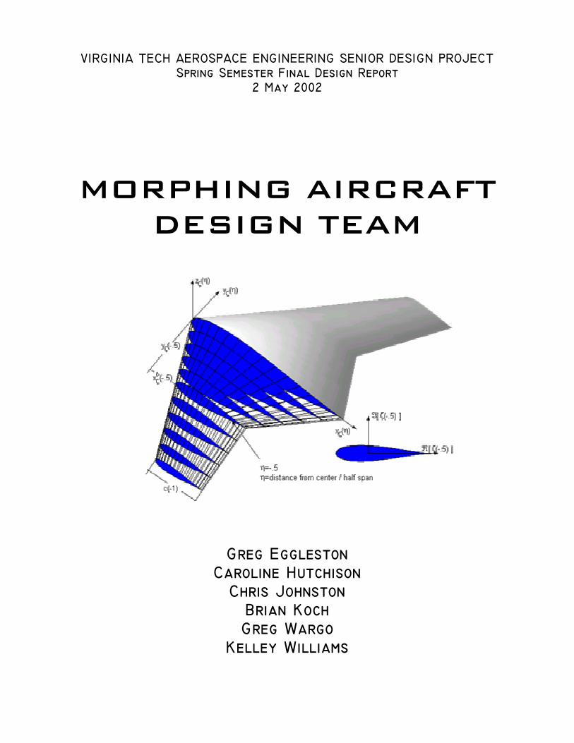
MORPHING AIRCRAFT DESIGN TEAM

Greg Eggleston Caroline Hutchison

Chris Johnston Brian Koch Greg Wargo

Kelley Williams

Table of Contents 1. Introduction 1 2. Overview of morphing concepts and past research 2 3. Design considerations 18

3.1. Initial Considerations 18 3.2. Minimum Drag Cruise Design 21 3.3. High-Lift Maneuver Design 25

4. Designs 27 4.1. Conventional Actuators (Servo Motors) 27 4.2. Shape Memory Alloys (SMA) 34 4.3. Piezoelectric Materials (PZTs) 47

5. Zagi testing 57 5.1. VLM Fortran Code 57 5.2. Tunnel testing 60 5.3 Results of ZAGI 400x Wind Tunnel Testing 65

6. Design testing 71 6.1. Comparison between the PZT and Servo Results. 73 6.2. Morphing Wind Tunnel Results. 77

7. Project conclusions 79 8. References 80 Appendices: 1. The MH 45 Airfoil 2. Introduction to the Morphing Wing Vortex Lattice Program 3. Construction Documentation for the PZT Model

1

Section 1. Introduction

December 17, 1903 the world’s first heavier-than-air, machine powered aircraft

leapt into the air in Kitty Hawk, North Carolina. That aircraft, The Wright Flyer,

featured ”wing warping” to achieve controlled flight. The wing warping system

consisted of a series of pulleys and cables that physically bent the wings. That method of

control is arguably a morphing wing. The word morph can be defined as “to cause to

change shape”. “Morphing” in the context of a wing’s geometry translates to a smooth

change in an aircraft’s physical characteristics. The Virginia Tech Morphing Wing

Design Team aims to design and build three model aircraft that each rely upon a unique

type of actuator to achieve the desired trailing edge shapes.

2

Section 2. An Overview of Morphing Concepts and Past Research

The ability of a lifting surface to alter its geometry during flight (i.e. morph) has

been of great interest to researchers and designers over the years. This is because a

morphing wing has the potential to decrease the number of compromises that a designer

is forced to make in order to assure that their aircraft is operational in multiple flight

envelopes. The trade-off between high-efficiency and high-maneuverability, as well as

the restriction of aerodynamic optimization for a single cruise condition, will no longer

be necessary.

Wing morphing is referred to with the following names throughout the research

literature: variable camber (VC) wings, mission adaptive wings, and smart trailing edge

wings. Throughout many parts of this report, the author may refer to morphing wings as

VC (variable camber) wings to emphasize that the camber is the main geometric feature

being modified. The use of this term narrows down the discussion to the consequences of

in-flight control of a wing’s camber at independent spanwise locations while maintaining

a smooth, continuous skin over the entire wing. The author found no research concerning

variable-sweep that used a smooth skin and independent spanwise control.

Subsonic Morphing

In the strictly subsonic flight regime, there are two main issues that promote the

use of a VC wing. The first of these, as explained by J.J. Spillman (Reference 1), stems

from the fact that the minimum drag at a given lift coefficient corresponds to an

increasing amount of airfoil camber. For example, at a CL of 0.80 and a Reynolds

number of 6-million, a NACA 4412 airfoil produces only 91% of the drag produced by

3

the 3% less cambered NACA 1412 airfoil (Reference 2). The 4412 section also has a

17% higher CL max at about the same stall angle of attack as the 1412 section. These

facts make it appear as if the 4412 section is superior to the 1412 section. But, below a

CL of 0.3, the drag for the 1412 is lower than of that for the 4412. So the desired camber

for high-lift or off-design situations disagrees with that desired for efficient high-speed

(subsonic, low CL) cruise. The introduction of variable-camber to this situation

eliminates these conflicting interests by allowing the airfoil to change its camber

depending on the flight situation. Although these airfoils are conventional, their

comparison shows the general effect of camber that will be present no matter how

advanced the airfoil.

The second primary benefit of VC wings for subsonic flight is the ability they

have to manipulate their spanload. For maximum cruise efficiency, the desired spanload

is most likely elliptic, although in some cases the wing-root bending moment of an

elliptic distribution forces a structural weight penalty that causes a net loss in total system

efficiency. In any case, the wing planform would be chosen so that it comes close to

producing the desired cruise spanload for the cruise CL. The planform that would be the

most efficient is usually not chosen because the planform must also produce a spanload

capable of satisfactory high-lift performance. This is a major factor for swept and

strongly tapered wings whose local CL values are highest towards the tip.

4

0 0.1 0.2 0.3 0.4 0.5 0.6 0.7 0.8 0.9 10.05

0.1

0.15

0.2

0.25

0.3

0.35

0.4

y/(b/2)

Cl

AR = 5.4 taper ratio = 0.354-degrees washout

Basic Lift (alpha dependent)

Additional Lift (not alpha dependent)

CL = 0.3 Alpha = 2 degrees

Total Lift = Basic + Additional

Maximum local Cl occurs at y/(b/2) = 0.45

Figure 2.1 Shows the components of the Cl distribution at a typical cruise condition.

Figure 2.1 shows an example of the CL distribution for a typical swept and tapered

wing in subsonic cruise (wing sweep for subsonic cruise is questionable, subsonic cruise

was examined because the calculation methods were available). This plot uses the linear

theory concept of basic (alpha-dependent) and additional (produced by the airfoil camber

and washout, non-alpha-dependent) lift. It is seen in the figure that a large portion of the

lift is non-alpha dependent, designed to produce the desired spanload at this alpha. This

also shifts the maximum CL value towards the root providing the illusion that the wing is

safe from wing-tip stall. The shifting of the maximum CL towards the root is discussed in

more detail next.

5

0 0.1 0.2 0.3 0.4 0.5 0.6 0.7 0.8 0.9 10

0.1

0.2

0.3

0.4

0.5

0.6

0.7

Cl

y/(b/2)

AR = 5.4 taper ratio = 0.354-degrees washout

Maximum local Cl occurs at y/(b/2) = 0.6

CL = 0.65Alpha = 7 degrees

Basic Lift (alpha dependent)

Total Lift

Additional Lift (not alpha dependent)

Figure 2.2 Shows the components of the Cl distribution at a high-lift or maneuver condition.

Figure 2.2 shows the same wing configuration at a higher alpha. It is seen that at

this alpha, the alpha-dependent lift begins to overshadow the unchanged non-alpha

dependent lift. The maximum CL value has moved from a y/(b/2) of 0.45 to 0.60. This

comparison showed just a 5-degree change in alpha. There are many flight situations

where a much larger alpha is required and examining the alpha-dependent lift shows that

this will continue to push the maximum CL location towards the tip.

6

0 0.1 0.2 0.3 0.4 0.5 0.6 0.7 0.8 0.9 10

0.1

0.2

0.3

0.4

0.5

0.6

0.7

0.8

Cl

y/(b/2)

Basic Lift (alpha dependent)

Maximum local Cl occurs at y/(b/2) = 0.4

Additional Lift (not alpha dependent)

CL = 0.65 Alpha = 7 degrees AR = 5.4 taper ratio = 0.354-degrees washout

2-degree control deflection at the root -1-degree control deflection at the tip

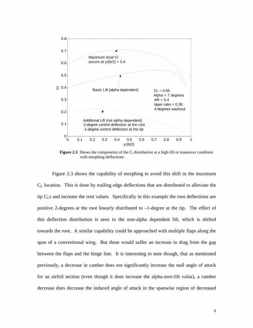
Figure 2.3 Shows the components of the Cl distribution at a high-lift or maneuver condition

with morphing deflections

Figure 2.3 shows the capability of morphing to avoid this shift in the maximum

CL location. This is done by trailing edge deflections that are distributed to alleviate the

tip CLs and increase the root values. Specifically in this example the root deflections are

positive 2-degrees at the root linearly distributed to –1-degree at the tip. The effect of

this deflection distribution is seen in the non-alpha dependent lift, which is shifted

towards the root. A similar capability could be approached with multiple flaps along the

span of a conventional wing. But these would suffer an increase in drag from the gap

between the flaps and the hinge line. It is interesting to note though, that as mentioned

previously, a decrease in camber does not significantly increase the stall angle of attack

for an airfoil section (even though it does increase the alpha-zero-lift value), a camber

decrease does decrease the induced angle of attack in the spanwise region of decreased

7

camber. So the positive effect of decreasing the camber in the regions of high values of

CL is the decrease in angle of attack that the endangered airfoils encounter, which puts

them further from their stall angle of attack and in less danger of stall. This load

redistribution towards the wing-root during high-lift situations also provides a decrease in

the wing-root bending moment. According to Reference 5, this would allow for a 10%

decrease in the structural weight of the wing.

Transonic Morphing

Variable camber implementation on transonic supercritical airfoils has been a

topic of considerable research. Although the performance of supercritical airfoils does

not significantly degrade for slight off-design conditions, the fact that a transonic aircraft

must do more than just cruise (i.e. take-off, climb, maneuver), forces multiple flight

conditions, or design points, to be considered in the airfoil design. This forces many

compromises, which lead to a decrease in the performance at each design point as

compared to what would be obtainable if only a single design point was considered in the

design. The main goal of past transonic morphing research has been to minimize these

compromises. The morphing methods that have been studied to achieve this are as

follows: 1) using variable-camber in the leading and trailing edges, 2) by using variable-

geometry on the upper surface of the airfoil. It should be noted that the subsonic

morphing methods discussed previously can still be used for transonic wing design to

satisfy design points in the subsonic flight regime.

The idea of using variable camber on the leading and trailing edges is very similar

to the concept mentioned for subsonic flight. There are increased benefits for using VC

at transonic speeds because of its ability to delay the formation of shocks, therefore

8

increasing the drag divergence Mach number. VC also delays the onset of buffet by

preventing total flow separation from occurring on the upper surface of the airfoil.

Reference 3 shows that these gains are a result of a VC wing’s ability to redistribute the

chordwise load for a given CL.

The purpose of leading-edge camber variation is to allow for a small leading-edge

curvature during low CL high-speed flight, and a large amount of curvature for high CL

low-speed flight and high angle of attack maneuvers. Trailing-edge camber is varied to

allow for the proper flow-recompression as determined by the flight condition. Trailing-

edge camber variation does have the drawback that it has large effect on the airfoils

pitching moment, and the potential to increase the trim drag. Reference 4 discusses in

depth the variation of the optimum trailing-edge shape with CL and Mach number. It

presents an example comparing the off-design performance of a fixed-camber airfoil to

one with a VC trailing edge. At the design Mach number and a CL that is 0.10 from the

design value, the VC airfoil produced 40% less drag than the fixed camber airfoil. For

the same change in off-design CL and with a Mach number that is 0.1 below the design

value, the VC airfoil produced about 60% less drag than the fixed-camber airfoil. The

superior performance of the VC airfoil at Mach numbers below its design value is a result

of its ability to simulate a decrease in camber through the use of trailing edge deflections.

The superior performance of the VC airfoil at off-design CL values is a result of its ability

to increase CL while maintaining a constant angle of attack (in other words it decreases its

alpha-zero-lift). The way in which this camber reduction or CL increase is produced

using the trailing edge is a very important matter at transonic speeds. Reference 4

determined the proper deflections through an optimization procedure requiring many

9

constraints. These included restricting the variable trailing edge section to 25% of the

chord, restricting deflection angles to 5-degrees, and using either one, two, or three

segments for the trailing edge. It was found that the number of trailing edge segments

made a significant difference in the drag at off-design lift CL values. On the other hand,

the decrease in drag at off-design Mach numbers was not very dependent on the number

of trailing edge segments.

There has been a considerable amount of research into the concept of using

variable-geometry on an airfoil’s upper-surface with the purpose of weakening shocks

that form at transonic flight speeds. This is different from using leading and trailing edge

deflections because this concept allows for independent chordwise variations in

thickness. Reference 3 provides an example of this concept by comparing the off-design

performance of a variable-geometry airfoil to that of a fixed geometry airfoil. Both

airfoils were designed for a CL = 0.5 at M = 0.78, while 90% of the variable geometry

upper surface was allowed to be adjusted using four actuator points. At the off-design

condition of M = 0.8, a 36% reduction in the off-design drag was found for the variable-

geometry airfoil over that of the fixed geometry airfoil. Using 8 actuator points on the

upper-surface allowed for an additional 8% decrease in drag at the off-design condition

over that of the fixed-geometry airfoil. The drag reduction of the variable-geometry

airfoil decreased by about a half when only 50% of the upper-surface was allowed to

change as opposed to 90% of the upper surface.

Reference 3 presents an interesting variable geometry concept that utilizes a

variable shape bump on the upper surface of the trailing edge in an attempt to weaken

shocks. The main difficulty with this concept is the optimum shape and location of the

10

bump change with Mach number. But this change in optimum shape and location is

tolerable considering the amount of trailing edge motion allowed for in the variable-

camber concept. Reference 3 shows that an effective range of chordwise motion for the

bump is about 10% of the chord, and the height can be limited to about 0.5 % of the

chord.

Past Morphing Research

The idea of morphing wings is nothing new; in fact as previously mentioned the

Wright brothers and many early airplane designers utilized wing warping (a form of

morphing) for roll control. As is pointed out by J.H. Renken (Reference 7), since the

1920s planes have regularly utilized high lift devices during take-off and landing. But as

airplanes became heavier, wings became stiffer thus using control surfaces (ailerons)

became more practical than wing warping. It wasn’t until the mid-70’s that morphing

wings began to be seriously considered and researched again. The majority of this

research was based on two morphing concepts, independent camber control along the

wingspan (variable camber), and flexible wings that used aeroelastic forces to obtain

beneficial wing deformations. The following section discusses these two morphing

methods.

Although the idea of VCWs is quite simple, actually designing the internal

variable camber devices and control systems that correctly utilize the variable camber

capability is very challenging. Many patents have been issued for the design of various

portions of internal variable camber devices. Patent 4,247,066, (Reference 8) shown in

Figure 2.4, was designed by Richard C. Frost, Eduardo W. Gomez, and Robert W.

11

McAnally of the General Dynamics Corporation of Fort Worth, Texas. The intent of this

device was to actuate the section aft of the wing box (number 38 in Figure 2.4), where a

conventional aircraft has its flaps and ailerons. It achieved a smooth, continuous

deflection by means of a “truss-like bendable beam” (number 26 in Figure 2.4) to which a

flexible skin was attached. The entire section was actuated by a series of jackscrews

(numbers 88 and 92 in Figure 2.4), which run chordwise through the structure. Upon

turning the jackscrews the upper and lower portions of the bendable beam move opposite

each other, giving a net deflection to the trailing edge of the structure.

Figure 2.4. Patent 4,247,066, Airfoil Variable Camber Device from General Dynamics, Forth Worth, Texas.

Another patent that concentrates on internal variable camber devices is United

States Patent 4,351,502 (shown in Figure 2.5), “Continuous Skin, Variable Camber

Airfoil Edge Actuating Mechanism.” This mechanism was invented by Frank D. Statkus

of the Boeing Company, Seattle Washington. Figure 2.5 shows how two sets of four bar

linkages are used in order to achieve a smooth camber change. One set to control the

12

horizontal and vertical motion of the main structure that defines the airfoil’s leading edge.

The second set controls the angle of rotation and the moment applied to the flexible skin

that envelopes the mechanism. According to the documentation (Reference 9), the design

criterion for this device require that uniform curvature in the chordwise direction for a

large range of deflections be maintained while; 1) keeping the flexible skin from

becoming a load bearing portion of the structure, i.e. it does not experience any additional

stresses due to the deflection induced by the internal mechanism 2) the system of four bar

linkages remain within the airfoil’s contour throughout the design deflection range and 3)

the structure can be integrated with the wing box without compromising the structural

stiffness of the wing box. The inventor commented on the percentage of the chord length

of an aircraft’s wing taken up by the wing box and trailing edge deflection apparatus,

approximately 80%. That leaves only 20% of the chord length for an actuating

mechanism for the leading edge. This limited amount of space available can lead to

compromises of the airfoil designer so that only a small range of optimal configurations

can be met. It is the argument of the designer of this mechanism that the system of four

bar linkages used overcomes the limitations of previous mechanisms which caused

discontinuities at high lift situations (i.e. flaps/slats) and increases the available range of

motion in a limited amount of space.

13

Figure 2.5 Patent 4,351,502, Continuous Skin, Variable Camber, Airfoil Edge Actuating Mechanism from the Boeing Company.

The previous two mechanisms were designed to allow an airfoil to smoothly

change shape so that it may operate at a range of optimal design conditions. Figure 2.6

shows a third patent that pertains to variable camber mechanisms. However, its

application does not place it in the wing of an aircraft. Patent 4,012,013, Variable

Camber Inlet for Supersonic Aircraft, was designed by William Henderson Bali and

Kichio Keith Ishimitsu of the Boeing Company. The inventors of this mechanism

intended for it to be integrated into the engine air inlet for supersonic aircraft. As the

speed of an aircraft increases from subsonic to supersonic the inlet area of the engine

must change in order to accommodate the changing needs of the engine. Usually the

inlets are designed for the optimal condition to be at the design cruise speed of the

14

aircraft. Thus, when the aircraft flies at off design conditions (i.e. subsonic speeds) a

large penalty is paid in engine performance and additional drag all due to the limited

flexibility of the inlet design. The variable camber mechanism designed by these

inventors allows the inlet area to smoothly vary, thus giving a larger range of optimal

design conditions at which the engine may run. As can be seen in Figure 2.6, this device

is broken into three “ramps”, fore, mid, and aft. In order to achieve a net deflection, each

ramp pivots around the ramp that is aft of its location. Therefore, the foremost ramp

pivots about the mid ramp, the mid ramp pivots about the aft ramp, and the aft ramp

pivots about the anchoring location. This invention shows that variable camber devices

are not only limited to increasing the performance of an airfoil.

Figure 2.6 Patent 4,012,013, Variable Camber Inlet for Supersonic Aircraft, from the Boeing Company.

15

In the mid-80’s Boeing set out to face the challenge of integrating both a variable

camber mechanism in the wings of an aircraft and a control system that would utilize the

variable camber to operate the aircraft at a range of optimal conditions. The AFTI/F-111

(Figure 2.7) used six independent trailing edge sections and two leading edge sections,

electro-hydraulic rotary actuators, and a flexible composite skin to achieve variable

camber. It took full advantage of its variable camber ability through the use of a flight

control system that used four operating modes for different optimization tasks. The

Maneuver Camber Control (MCC) mode selected the best leading and trailing edge

contour to maximize lift to drag efficiency. This was done by a computer, which

measured the dynamic pressure, normal acceleration, Mach number, and fuel volume and

then consulted stored data tables to give it the corresponding leading and trailing edge

contours. Cruise Camber Control mode (CCC) was designed to maximize velocity at

constant altitude and throttle setting. This closed loop mode performed an iterative

process of changing the trailing edge camber until the maximum velocity was achieved.

Maneuver Load Control mode (MLC) measured the wing root bending moment and

adjusted the camber on the outboard wing in order to move more of the wing loading

towards the root. Maneuver Enhancement/Gust Alleviation (MEGA) was designed to

quicken airplane response. The MEGA used a complex computer process which will not

be explained in this paper, but more information about it can be found in Reference 11.

Flight tests of the AFTI/F-111 confirmed the effectiveness of VCWs by

demonstrating a 20-30 percent increase in mission range, 20 percent in lift to drag

efficiency and 15 percent increase in wing load at constant bending moment (Reference

12).

16

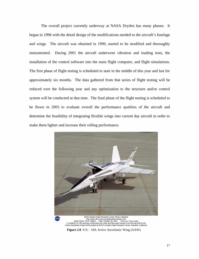
Figure 2.7 AFTI F-111 Mission Adaptable Wing in Flight.

The use of aerodynamically induced wing twist for a roll maneuver is the most

recent area of research in morphing technology. NASA Dryden with the United States

Air Force and Boeing’s Phantom Works is currently working on the Active Aeroelastic

Wing (AAW) flight research project. This concept has been billed as revisiting the “wing

warping” concept that the Wright Brothers used in their Flyer. The Wright Brothers,

using a system of cables and pulleys physically bent or “warped” their wings in order to

roll their craft. For the AAW project an F/A-18A has been specially modified (shown in

Figure 2.8) and was “rolled-out” on March 27th of this year (2002). The main wing skin

panels were replaced with thinner, lighter panels and the leading edge flap was divided

into an inboard and outboard section. Through the use of the outboard flap on the leading

edge and the aileron on the trailing edge to twist the wing, the aerodynamic forces that

result from the twisted wing will result in the forces necessary to roll the aircraft.

17

The overall project currently underway at NASA Dryden has many phases. It

began in 1996 with the detail design of the modifications needed to the aircraft’s fuselage

and wings. The aircraft was obtained in 1999, started to be modified and thoroughly

instrumented. During 2001 the aircraft underwent vibration and loading tests, the

installation of the control software into the main flight computer, and flight simulations.

The first phase of flight testing is scheduled to start in the middle of this year and last for

approximately six months. The data gathered from that series of flight testing will be

reduced over the following year and any optimization to the structure and/or control

system will be conducted at that time. The final phase of the flight testing is scheduled to

be flown in 2003 to evaluate overall the performance qualities of the aircraft and

determine the feasibility of integrating flexible wings into current day aircraft in order to

make them lighter and increase their rolling performance.

Figure 2.8 F/A – 18A Active Aeroelastic Wing (AAW).

18

Section 3. Design Considerations for the Morphing Wing

This section will discuss the basic configuration, and the reasoning for it, of the

final design of the morphing wing.

Section 3.1. Initial Considerations

Prior to any aerodynamic analysis a flying wing configuration was selected as the

final layout. This configuration led to some interesting design issues, not normally

addressed with a conventional aircraft which features a tail. Once the aerodynamic

analysis was begun it used the same airfoil and planform as the Zagi 400X (taper ratio =

0.52, AR = 4.8, LE sweep = 30 deg., the MH-45 airfoil is discussed in Appendix 1), a

proven flying wing design. These early decisions allowed the majority of the

aerodynamic design to be focused on figuring out the optimal wing shape for various

flight conditions. Early weight and speed estimates allowed a design CL of 0.3 to be

chosen. To aid in the design process, a vortex lattice program was written for easy

analysis of various designs. This program is presented in Appendix 2 and was used to

generate the aerodynamic information presented in this section.

It was decided that the flying wing would be balanced stable to eliminate the need

for a stability augmentation system. This decision had a strong influence on the way the

control surfaces would have to be deflected to achieve trimmed flight. The main design

issue that arose from this was finding the combination of control deflections and wing

twist that produced the design CL while creating no pitching moment and minimizing

drag.

The vortex lattice program was written especially to allow for a quick and easy

estimate of a wide range of control deflections. It was known that a vortex lattice method

19

is not very accurate at predicting the influence of deflected control surfaces because of its

over-prediction of the control surface effectiveness. From the comparison of wind-tunnel

tests to the VLM predictions of the Zagi 400X, it was found that the aerodynamic

characteristics predicted by the VLM for an elevon deflection, was equal to the wind

tunnel results for a control deflection that was 1.6 times the deflection predicted by the

VLM code. This correction factor was used for this design, although it was hoped that

the smooth control surfaces of the morphing wing would improve the control

effectiveness from that of the Zagi and therefore improve the VLM accuracy. The most

important aspect of the VLM program was its prediction of spanloads, and the effect of

control deflections on these spanloads. The spanloads were used to calculate the induced

drag, so they were very important in finding the deflections that produced the least

induced drag.

The control deflections necessary for trimmed flight at a CL = 0.3 were examined

first along with the optimal washout and number of independent spanwise control

stations. For a given number of spanwise control stations and a washout value, the

control deflections necessary for the highest efficiency spanload possible were found

through a manually iterative process of choosing deflections that minimized the

difference between the spanload and an ideal elliptic spanload of the same lift coefficient.

Fig. 3.1 shows the dependence of the maximum obtainable spanload efficiency factor on

the number of spanwise control segments. This plot does not show the negative influence

of the weight increase that occurs as more spanwise control segments are added. The

servo group decided upon six control segments for each half span. Fig. 3.2 shows the

influence of washout on the spanload efficiency factor. By comparing the peaks of the

trimmed and untrimmed line, the trim requirement can be seen to increase the desired

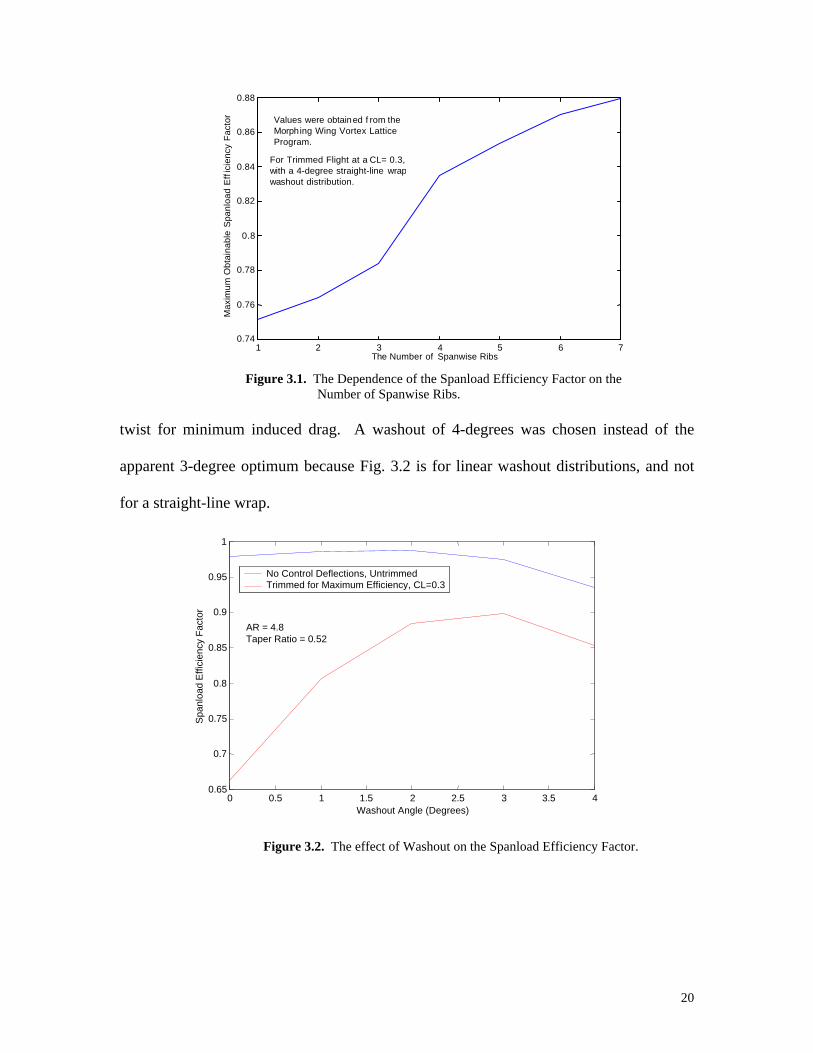
20

Figure 3.1. The Dependence of the Spanload Efficiency Factor on the Number of Spanwise Ribs.

twist for minimum induced drag. A washout of 4-degrees was chosen instead of the

apparent 3-degree optimum because Fig. 3.2 is for linear washout distributions, and not

for a straight-line wrap.

0 0.5 1 1.5 2 2.5 3 3.5 4 0.65

0.7

0.75

0.8

0.85

0.9

0.95

1

Washout Angle (Degrees)

Spa

nloa

d E

ffici

ency

Fac

tor

No Control Deflections, Untrimmed Trimmed for Maximum Efficiency, CL=0.3

AR = 4.8 Taper Ratio = 0.52

Figure 3.2. The effect of Washout on the Spanload Efficiency Factor.

1 2 3 4 5 6 70.74

0.76

0.78

0.8

0.82

0.84

0.86

0.88

The Number of Spanwise Ribs

Max

imum

Obt

aina

ble

Spa

nloa

d E

ffic

ienc

y F

acto

r

For Trimmed Flight at a CL= 0.3,with a 4-degree straight-line wrapwashout distribution.

Values were obtained f rom theMorphing Wing Vortex LatticeProgram.

21

The straight-line wrap, shown in Fig. 3.3, was found to be favorable because it

would make construction of the wing much easier, and because it focused more of the

twist towards the tip, where it had more influence on the pitching moment.

0 0.1 0.2 0.3 0.4 0.5 0.6 0.7 0.8 0.9 1 0

0.5

1

1.5

2

2.5

3

3.5

4

y/(b/2)

Tw

ist A

ngle

(de

gree

s)

Figure 3.3. Straight-Line Wrap Twist Distribution.

Section 3.2. Minimum Drag Cruise Design

For the design CL of 0.3, a straight-line wrap washout of 4-degrees, and six

spanwise ribs, the control deflections necessary for trimmed flight with the minimum

possible induced drag are shown in Table 3.1. The resulting spanload is shown in Figure

3.4, along with the desired elliptic spanload and the spanload obtained when a

conventional one-piece elevon is deflected for trimmed flight at a CL of 0.3. It is seen

that the design spanload cannot quite match the elliptic shape for trimmed flight.

22

0 0.1 0.2 0.3 0.4 0.5 0.6 0.7 0.8 0.9 1 0.4

0.5

0.6

0.7

0.8

0.9

1

1.1

C l

y/(b/2)

Wing morphed for the high-lift. Trimmed at 12-deg AOA.

Conventional one-piece elevon deflected to -2.7 deg. Trimmed at 12-deg AOA. C L = 1.0

C L = 1.1

Table 3.1. Cruise Deflection Distribution.

The benefit of independent spanwise control is seen in Fig. 3.4 by observing the

one-piece elevon’s poorly shaped spanload and corresponding e of 0.77. The poor results

are slightly misleading because the elevon was not shaped for a CL of 0.3. A one piece

elevon could be designed to produce a spanload similar to the variable camber’s at the

design CL, but away from the design point its performance would drop quickly from that

obtainable by variable camber.

Figure 3.4. Trimmed Spanloads.

Cruise Deflection Distribution Rib # Deflection (deg)

1 Root -3.1 2 -2.4 3 -1.6 4 -0.8 5 -0.5

6 Tip -0.3

23

To account for small changes in the required CL and to allow for mild maneuvers,

the control system was designed to deflect the control deflections away from the cruise

configuration in a way that kept drag to a minimum but also shifted the CM0L enough to

shift the trimmed CL. This was done by finding the trimmed, minimum drag control

deflections for CL values ranging from 0.45 to 0.20. For each spanwise rib, a line was

then fit through the required deflection from the cruise configuration to obtain the various

trimmed, off design CL values. The slope of these lines were then programmed into the

control system so that any pitch commanded by the pilot, would be produced by the wing

using minimum drag control deflections. In other words, for the cruise mode, the

independent spanwise control segments always moved away from the cruise

configuration with same ratio of deflection angles relative to each other. These ratios are

shown in Table 3.2. It is important to remember that these ratios are not appropriate for

significant maneuvers or for high-lift situations because they were not designed with

wing tip stall in mind. The control system was designed so that if a pitch command

required a control segment to move more than 5-degrees away from the cruise

configuration, the set of ratios used by the control system would switch to ones that were

designed for high-lift and maneuvers. These ratios will be discussed in the next section.

Table 3.2. Control Surface Motion for Small Changes in CL.

Control Surface Motion for Small Changes in CL

Ratio of Motion from Rib # the Cruise Configuration

1 Root 0 2 0 3 0 4 -0.75 5 -1

6 Tip -1

24

Before ending this section on the cruise design, it should be noted that without the

trim condition, an elliptic spanload is easily obtained with the right control deflections.

In the case of a tailed aircraft with variable camber, this elliptic spanload could be used,

but then the required CL would have to be slightly greater to compensate for the negative

trim lift generated by the horizontal tail. This increased CL would lead to an increase in

induced drag. So which increase in induced drag due to trim requirements is greater, that

caused by a flying wing’s distorted spanload, or that caused by a tailed aircraft’s increase

in required CL? The effect of the control deflections on the trimming the aircraft are

shown in Figure 3.5.

Figure 3.5. Trim Analysis.

Figure 3.5. Trim Requirements of a Flying Wing

Section 3.3. High-Lift and Maneuver Design

It was mentioned previously that it is possible for a one-piece elevon to match the

cruise performance of a morphing wing. For high-lift and maneuver conditions though,

the morphing performance becomes unobtainable for the one-piece elevon. This is

-0.06

-0.05

-0.04

-0.03

-0.02

-0.01

0

0.01

0.02

-0.4 -0.2 0 0.2 0.4 0.6 0.8 1CL

CM

4-Degrees Washout

T. E. Deflections

Trimmed CL

Planar, Cambered Planform

Morphing-SpecificVLM predictions

25

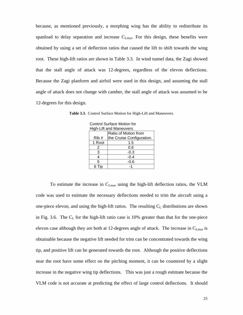
because, as mentioned previously, a morphing wing has the ability to redistribute its

spanload to delay separation and increase CLmax. For this design, these benefits were

obtained by using a set of deflection ratios that caused the lift to shift towards the wing

root. These high-lift ratios are shown in Table 3.3. In wind tunnel data, the Zagi showed

that the stall angle of attack was 12-degrees, regardless of the elevon deflections.

Because the Zagi planform and airfoil were used in this design, and assuming the stall

angle of attack does not change with camber, the stall angle of attack was assumed to be

12-degrees for this design.

Table 3.3. Control Surface Motion for High-Lift and Maneuvers.

To estimate the increase in CLmax using the high-lift deflection ratios, the VLM

code was used to estimate the necessary deflections needed to trim the aircraft using a

one-piece elevon, and using the high-lift ratios. The resulting CL distributions are shown

in Fig. 3.6. The CL for the high-lift ratio case is 10% greater than that for the one-piece

elevon case although they are both at 12-degrees angle of attack. The increase in CLmax is

obtainable because the negative lift needed for trim can be concentrated towards the wing

tip, and positive lift can be generated towards the root. Although the positive deflections

near the root have some effect on the pitching moment, it can be countered by a slight

increase in the negative wing tip deflections. This was just a rough estimate because the

VLM code is not accurate at predicting the effect of large control deflections. It should

Control Surface Motion for High-Lift and Maneuvers

Ratio of Motion from Rib # the Cruise Configuration.

1 Root 1.5 2 0.6 3 -0.3 4 -0.4 5 -0.6

6 Tip -1

26

0 0.1 0.2 0.3 0.4 0.5 0.6 0.7 0.8 0.9 1 0.4

0.5

0.6

0.7

0.8

0.9

1

1.1

C l

y/(b/2)

Wing morphed for the high-lift. Trimmed at 12-deg AOA.

Conventional one-piece elevon deflected to -2.7 deg. Trimmed at 12-deg AOA. C L = 1.0

C L = 1.1

be noted that the reasoning given above for the increase in CLmax could be applied to a

two-piece conventional flap system. But, it is hoped that the wind tunnel testing will

show that the smooth continuous surface of the variable camber system will put less

strain on the boundary layer therefore allowing a larger recompression without flow

separation.

Figure 3.6. Cl Distributions for Trimmed Flight at the Stall AOA.

27

Section 4. Morphing Methods Researched by the Virginia Tech Morphing Wing

Design Team

The Virginia Tech Morphing Wing Design Team has developed three different

flying wing models. Each model utilizes a different type of actuator to morph the wing.

Each model had a dedicated group of engineers who developed the concept into the full

scale model. The three groups are; Conventional Actuators (servomotors), Shape

Memory Alloys (Nitinol), and Piezoelectric Materials (PZTs). Each group’s model is

discussed in the following sections.

Section 4.1 Conventional Actuators

The use of servo motors is one of the three methods utilized to achieve the desired

morphing capabilities. Servos are small rotary motors that can produce large torques

with minimal current draw and space requirements. The response time of a servo is

almost instantaneous, so control lag is not a design issue. A cut-away picture of a servo

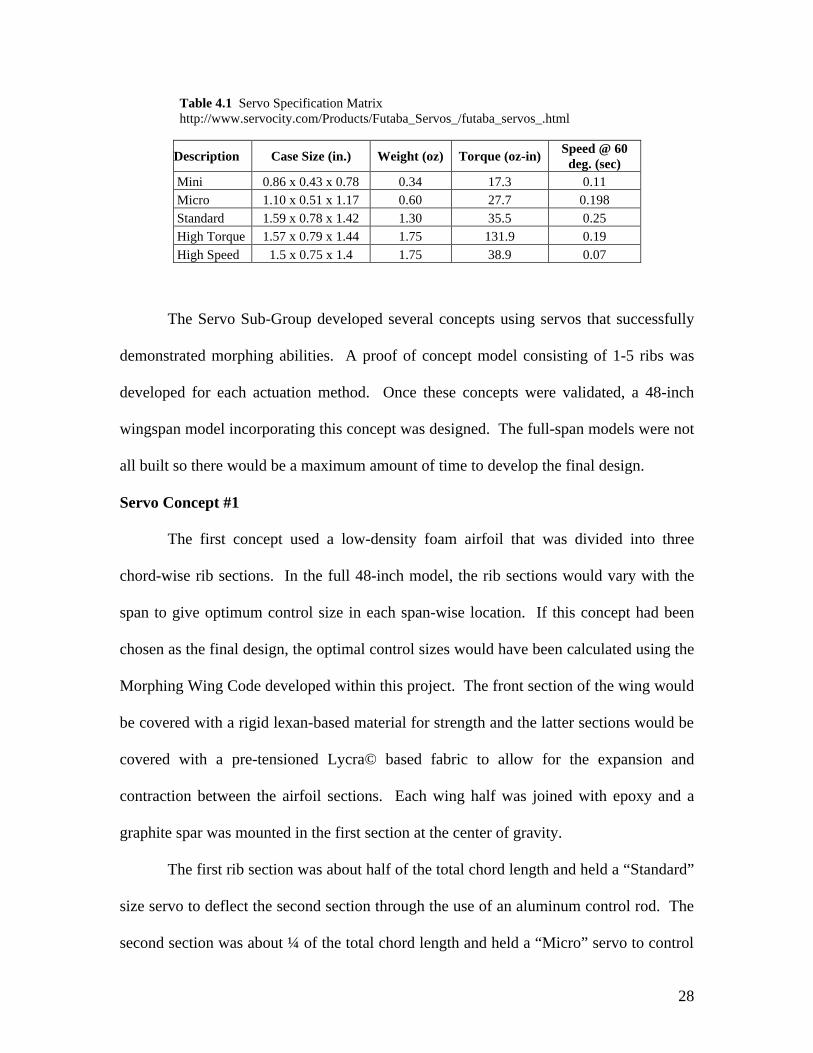
is shown in Figure 4.1 and sample data for the servos used in this concept are shown in

Table 4.1.

Figure 4.1. Servo Cut-away. http://www.servocity.com/Products/Futaba_Servos_/futaba_servos_.html

28

Table 4.1 Servo Specification Matrix http://www.servocity.com/Products/Futaba_Servos_/futaba_servos_.html

The Servo Sub-Group developed several concepts using servos that successfully

demonstrated morphing abilities. A proof of concept model consisting of 1-5 ribs was

developed for each actuation method. Once these concepts were validated, a 48-inch

wingspan model incorporating this concept was designed. The full-span models were not

all built so there would be a maximum amount of time to develop the final design.

Servo Concept #1

The first concept used a low-density foam airfoil that was divided into three

chord-wise rib sections. In the full 48-inch model, the rib sections would vary with the

span to give optimum control size in each span-wise location. If this concept had been

chosen as the final design, the optimal control sizes would have been calculated using the

Morphing Wing Code developed within this project. The front section of the wing would

be covered with a rigid lexan-based material for strength and the latter sections would be

covered with a pre-tensioned Lycra© based fabric to allow for the expansion and

contraction between the airfoil sections. Each wing half was joined with epoxy and a

graphite spar was mounted in the first section at the center of gravity.

The first rib section was about half of the total chord length and held a “Standard”

size servo to deflect the second section through the use of an aluminum control rod. The

second section was about ¼ of the total chord length and held a “Micro” servo to control

Description Case Size (in.) Weight (oz) Torque (oz-in) Speed @ 60 deg. (sec)

Mini 0.86 x 0.43 x 0.78 0.34 17.3 0.11 Micro 1.10 x 0.51 x 1.17 0.60 27.7 0.198 Standard 1.59 x 0.78 x 1.42 1.30 35.5 0.25 High Torque 1.57 x 0.79 x 1.44 1.75 131.9 0.19 High Speed 1.5 x 0.75 x 1.4 1.75 38.9 0.07

29

the deflection of the trailing edge section. The three sections were joined with a fiber-

paper hinge. The interior sides of the sections were cut so that a +45o deflection was

possible between each section. Several sets of servos could be placed along the span to

give different possibilities for trailing edge shapes.

The benefits to this concept were that it would be very lightweight, cheap, and

easy to produce. Since the deflection of each section was independently controlled, many

deflection combinations could be achieved such as: aileron, flap, + reflex, airbrake,

rudder, high lift, and maximum lift curve efficiency.

One apparent disadvantage to this design was that the actuations stressed the

joints and after extreme use, the hinges could conceivably fail due to fatigue.

Servo Concept #2

The second servo concept used a 1/8” fiberboard duplicate of the airfoil and servo

setup as the first concept, but utilized a high-impact plastic chain and gear drive system.

This setup used metal pin hinges between rib sections. The actuating gear would be

placed on the hinge to enable rotation about that point. The same coverings were to be

used with this concept, but foam fillers would be fitted between ribs. Two long carbon

fiber spars would connect the ribs together.

One advantage of this actuation system is that the chains tolerated large amounts

of tension before considerable elongation. The chain configuration also provided faster

and smoother response between sections. The pull-pull drive system also minimized the

joint fatigue problem with the first concept. Another advantage to this system was that

the gear sizes can be varied to tailor the deflections of each section.

30

One disadvantage of this system was the possibility of the chains breaking or

losing tension during flight. Also, if the chains needed to be maintained, the wing

covering would need to be removed, which may require a significant amount of effort.

Another difficulty of this design is joint-slop resulting from the torque on the gears.

Shown below (Fig 4.2) is a picture of one chain-actuated rib. The chord length of the rib

is 12 inches.

Figure 4.2. Picture of Servo Concept #2 and Chain Specifications. http://www.servocity.com/Products/Plain_Bore_Sprockets/Chain_Specifications/chain_specifications.html

Servo Concept #3

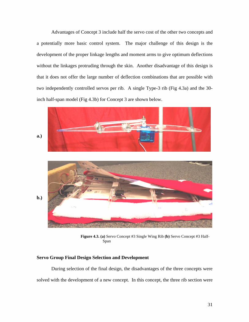
The third servo-actuated morphing concept used linearly-actuated ribs. A 30-inch, half-

span model was built for this concept. Each rib still had three sections, but a single servo

mounted in the first section controlled each trailing section through a complex linkage

system. Five actuated ribs were placed along the model’s span and covered with the

same materials as the other two concepts. In order to have a smooth trailing edge when

the ribs were deflected, lightweight, flexible Styrofoam was cut to match the third airfoil

section and placed between the ribs. The foam was flexible enough to conform to the

deflected position, yet strong enough to maintain a smooth line at the trailing edge.

31

Advantages of Concept 3 include half the servo cost of the other two concepts and

a potentially more basic control system. The major challenge of this design is the

development of the proper linkage lengths and moment arms to give optimum deflections

without the linkages protruding through the skin. Another disadvantage of this design is

that it does not offer the large number of deflection combinations that are possible with

two independently controlled servos per rib. A single Type-3 rib (Fig 4.3a) and the 30-

inch half-span model (Fig 4.3b) for Concept 3 are shown below.

a.) b.)

Figure 4.3. (a) Servo Concept #3 Single Wing Rib (b) Servo Concept #3 Half-Span

Servo Group Final Design Selection and Development

During selection of the final design, the disadvantages of the three concepts were

solved with the development of a new concept. In this concept, the three rib section were

32

joined and actuated by two servos. The servos were placed at the joints so that the

following rib section was mounted on the previous servo’s head. This method gave the

precision of the chain-driven model without the difficulties associated with it. With this

“direct drive” concept, there was no chance of the linkages protruding through the skin

since there were no linkages. The only possibly disadvantage of this concept is that all

the mechanical and aerodynamic forces are transmitted directly to the servo’s gears. In

the linked models, the forces could be reduced through gearing. If overwhelming forces

were experienced, the internal servo gears would strip, resulting in replacement of the

servo.

This design would be the fastest and easiest to build, with the lowest possibilities

for malfunction. Due to the benefits of this design and lack of significant disadvantages,

it was unanimously chosen as the final design.

The final design incorporated the “direct drive” actuation and the following

features:

• Removable wing-halves • Dual carbon fiber spars • 16 independently operated servos • 8 dual-actuating ribs, 4 single-joint ribs (2 nearest each tip) • Microprocessor controls • High-density EPP foam leading section, flexible foam trailing edge section • Surgical grade latex skin over aft 75% of airfoil • Electronics “floor” at root for wing and electronics mounting • Aerodynamic fiberglass cowling over root section fitted for fuel tank • O.S. 0.46 cc LA glow engine – 2 cycle with 10 x 6 prop

Figure 4.4 shows the starboard wing as it looks without skin when detached from the

center section.

33

Figure 4.4. Assembled wing half for Servo final model.

The control system for this design had two configurations: hard-wire and remote operation. The hard-wire system uses a control program developed in Visual Basic to actuate the servos. The code output from a PC was wired to a pair of servocontrollers mounted on the electronics floor of the aircraft. The command window for the hard-wire control program is shown in figure 4.5. The servos were connected to the servocontrollers. The remote system used the same servocontrollers. A standard R/C transmitter sends a signal to the corresponding receiver. A PIC microprocessor translated the data from the receiver and sent the flight data to the servocontrollers.

34

Section 3.2 Shape Memory Alloys

The term Shape Memory Alloys (SMA) is applied to a group of metallic materials

that demonstrate the ability to return to some previously defined shape or size when

subjected to the appropriate thermal procedure. The shape memory effect is caused by a

temperature dependent crystal structure. When an SMA is below its phase

transformation temperature, it possesses a low yield strength crystallography referred to

as Martensite. While in this state, the material can be deformed into other shapes with

relatively little force. The new shape is retained provided the material is kept below its

transformation temperature. When heated above this temperature, the material reverts to

its parent structure known as Austenite causing it to return to its original shape and

rigidity. These transformations can be further understood by looking at Figure 4.6,

below.

Figure 4.6. Charts Depicting Different State of Shape Memory Alloys http://www.sma-inc.com

This phenomenon can be harnessed to provide a unique and powerful actuator.

Materials that exhibit shape memory only upon heating are referred to as having a one-

way shape memory. The ability of shape memory alloys to recover a preset shape upon

35

heating above the transformation temperatures and to return to a certain alternate shape

upon cooling is known as the two-way shape memory effect.

The first recorded observation of the shape memory transformation was by Chang

and Read in 1932. They noted the reversibility of the transformation in AuCd by

metallographic observations and resistivity changes, and in 1951 the shape memory effect

was observed in a bent bar of AuCd. In 1938, the transformation was seen in brass

(CuZn). In the early 1960s, Buehler and his co-workers at the U.S. Naval Ordnance

Laboratory discovered the shape memory effect in an equiatomic alloy of nickel and

titanium, which can be considered a break through in the field of shape memory

materials. This alloy was named Nitinol (Nickel-Titanium Naval Ordnance Laboratory).

Since that time, intensive investigations have been made to clarify the mechanics of its

basic behavior. The use of Nitinol for medical applications was first reported in the

1970s. It was only in the mid-1990s, however, that the first widespread commercial

applications made their breakthrough in medicine. The use of Nitinol as a biomaterial is

fascinating because of its superelasticity and shape memory effect, which are completely

new properties compared to the conventional metal alloys.

Although a relatively wide variety of alloys are known to exhibit the shape

memory effect, only those that can recover substantial amounts of strain or that generate

significant force upon changing shape are of commercial interest. To date, this has been

the nickel-titanium alloys and copper-base alloys such as CuZnAl and CuAlNi. The most

widely used shape memory material is the alloy of Nickel and Titanium called Nitinol.

This particular alloy has excellent electrical and mechanical properties, long fatigue life,

and high corrosion resistance. As an actuator, it is capable of up to 5% strain and 50,000

36

psi recovery stress, resulting in approximately 1 Joule/gm of work output. Nitinol is

readily available in the form of wire, rod, and bar stock with transformation temperature

in the range of -100º to +100º Celsius. Due to these reasons, our design group decided to

use Nitinol for all of our applications.

There are limitations of shape memory. About 8% strain can be recovered by

unloading and heating. Strain above the limiting value will remain as a permanent plastic

deformation. The operating temperature for shape memory devices must not move

significantly away from the transformation range, or else the shape memory

characteristics may be altered. The two-way shape memory effect is a very hard

phenomenon to use. Creating two-way memory in NiTi alloys involves a somewhat

complex training process. The amount of recoverable strain is generally about 2%, which

is much lower than that which is achievable in one-way memory (6 to 8%). The

transformation forces upon cooling are extremely low and the memory can be erased with

very slight overheating.

Wherever possible, it is better to modify the device design to make use of one-

way memory with a biasing force acting against the shape memory element to return it

upon cooling. Two-way actuators using one-way shape memory elements acting against

bias forces have demonstrated large strains, high forces in both heating and cooling

directions, and excellent long-term stability up to millions of cycles. Therefore our

design group decided to use the one-way shape memory effect to our advantage.

To further understand this new technology we had to construct relatively crude

models in order to visualize these properties. After this was done, we could begin

looking into different design concepts that we came up with at various meetings. Once

37

we narrowed these concepts down to the ones that we felt would benefit our aircraft the

most, we created simple models to prove the concept we were trying to use. If the

concept worked as we wanted, then we moved on to build a more intricate and

representative model to show the rest of the design group and use in presentations. The

SMA subgroup has two finalized models, which it feels portray each design concept well.

There are two design concepts with shape memory alloy materials incorporated

into them help to morph camber and help twist the wing. The camber model shown

below in Figure 4.7 demonstrates how Nitinol can be used to change the camber of a

wing. The model is composed of a polyurethane rod mounted to a wooden support that

represents the wing box. Four Flexane sheets were attached to the rod to break the airfoil

shape into sections. You can see below that the Nitinol wire is woven between the

Flexane sheets.

Figure 4.7. Shape Memory Alloy Concept Creating a Camber Change.

Both wires (top and bottom) are pre-strained, by pre-straining them, so that when

heated they will shrink back to their original length. By providing an electrical current to

the bottom wires they will heat up to the prescribed transformation temperature and

38

shrink. The rod adds a biasing force, by means of its internal energy, to help return the

airfoil to its natural shape upon cooling and actuation of the opposite wires. The only

drawback is that the deflection isn’t always in the desired plane because the circular

cross-section of the rod enables it to move in all directions. Lateral connections would

just hinder the movement of the rib in the direction that we need. By replacing the rod

with a different material, such as a wide sheet of stiff aluminum, the model would behave

as it was designed to do. Nonetheless, it has been demonstrated that Nitinol can be used

to change the camber of a wing.

Figure 4.8. Shape Memory Alloy Concept Creating Wing Twist.

The other model that was constructed demonstrates how to twist the wing, see

figure 4.8. This model is composed of a wooden base with a stiff rubber tube attached to

it. Nitinol wires were connected from the base to a PVC pipe attached to a wooden rod.

The wooden rod goes through the rubber tube and is connected at the end. By actuating

one set of wires the PVC pipe will rotate, moving the wooden rod. This causes the

39

rubber tube to rotate more at the end than at the base. This represents a variable twist,

more at the wing tip than at the wing root. The airfoils cut out of pink foam help

visualize this twisting effect. This model has been wired so that the actuation can be

controlled from the small switch box on the front left of the model. This model

successfully displays how variable twist can be used on an aircraft by use of Nitinol.

This design team has addressed many different concepts incorporating the usage

of shape memory alloys. The concepts described so far in this report are possibilities for

implementation of our morphing aircraft, and for further study. At the beginning of the

spring semester, the SMA sub-group discussed what method of morphing to incorporate

into our final design project. We decided that a method to change only the camber would

suffice. By placing several ribs that could change the camber along the span we could in

effect create twist also. We therefore adopted the method of actuation pictured in figure

4.6 to act as a basis of our design.

There were several problems with this woven model that needed to be considered.

It was exceptionally complicated to build, especially if we have to build a large number

of them. It was also too thick of a design to fit inside of the airfoil. However, the

concept had some potential that we wanted to further explore. This led us to attempt to

alter the design to make it thinner and simpler. We decided that the thinnest we could

make a rib was to practically lay the Nitinol wiring on top of the rib itself. In order to do

this we would have to use a flat rectangular cross-section comprised of a non-conductive

material. We decided to use Plexiglas for this purpose. By making crude models for

proof of concept purposes, we proved that this could be done successfully. The main

problem encountered was the tremendous heat of the wire as a result of the large amount

40

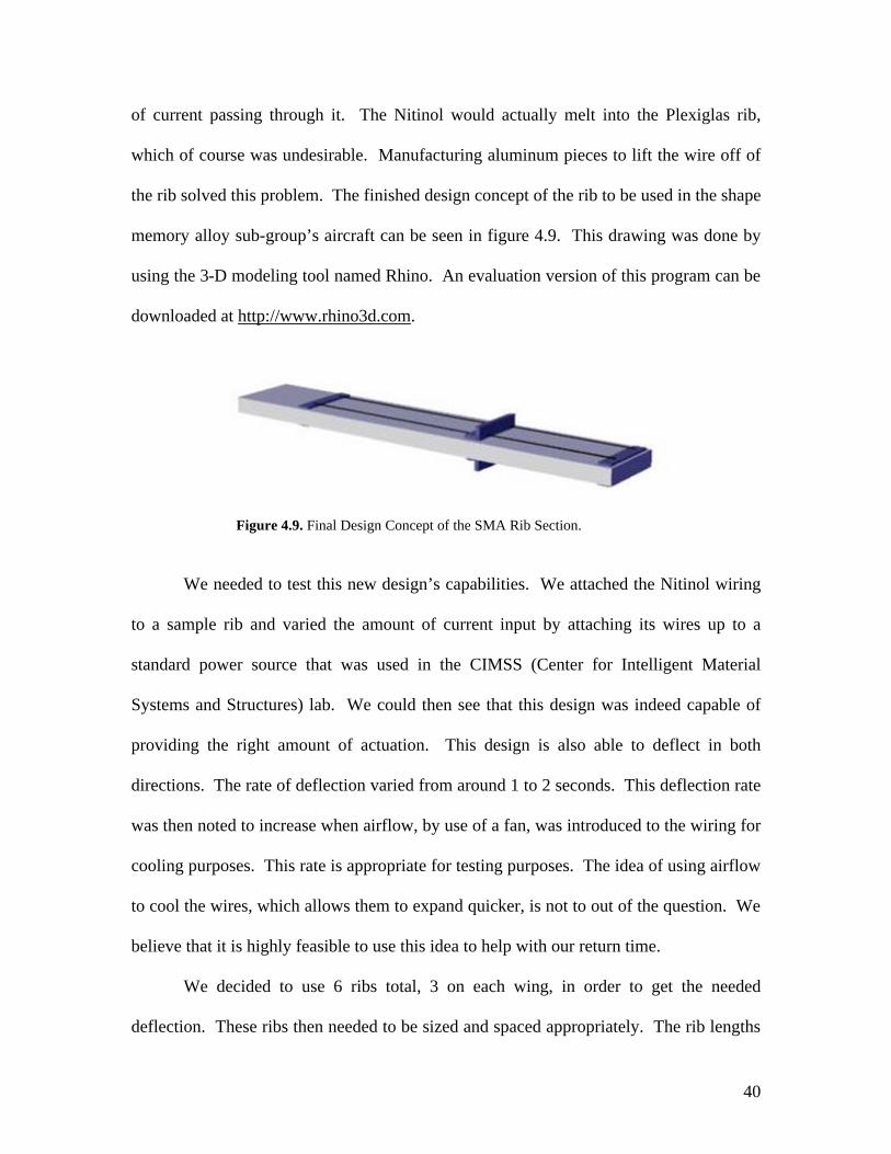
of current passing through it. The Nitinol would actually melt into the Plexiglas rib,

which of course was undesirable. Manufacturing aluminum pieces to lift the wire off of

the rib solved this problem. The finished design concept of the rib to be used in the shape

memory alloy sub-group’s aircraft can be seen in figure 4.9. This drawing was done by

using the 3-D modeling tool named Rhino. An evaluation version of this program can be

downloaded at http://www.rhino3d.com.

Figure 4.9. Final Design Concept of the SMA Rib Section.

We needed to test this new design’s capabilities. We attached the Nitinol wiring

to a sample rib and varied the amount of current input by attaching its wires up to a

standard power source that was used in the CIMSS (Center for Intelligent Material

Systems and Structures) lab. We could then see that this design was indeed capable of

providing the right amount of actuation. This design is also able to deflect in both

directions. The rate of deflection varied from around 1 to 2 seconds. This deflection rate

was then noted to increase when airflow, by use of a fan, was introduced to the wiring for

cooling purposes. This rate is appropriate for testing purposes. The idea of using airflow

to cool the wires, which allows them to expand quicker, is not to out of the question. We

believe that it is highly feasible to use this idea to help with our return time.

We decided to use 6 ribs total, 3 on each wing, in order to get the needed

deflection. These ribs then needed to be sized and spaced appropriately. The rib lengths

41

were found by using the length of the cord left between the spar and the trailing edge.

The distances between the individual components were designed to provide the

appropriate moments needed for deflection. Please refer to figure 4.10 below to see the

design specifications of the ribs.

Figure 4.10. Construction Layout of the SMA Ribs

Now that there was a definite way to induce deflection, we needed to design how

to incorporate this into an aircraft structure. The first thing to be done was to figure out

how to attach the ribs to the aircraft. This was done by creating a bottom spar structure

made of 1/4” birch plywood, cut out so that there was an area large enough to mount the

electronics and sturdy enough to attach the ribs. Once the ribs are bolted onto this

structure, another spar is placed on top to secure them in place and to provide the

42

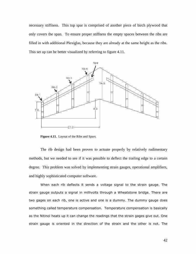
necessary stiffness. This top spar is comprised of another piece of birch plywood that

only covers the span. To ensure proper stiffness the empty spaces between the ribs are

filled in with additional Plexiglas, because they are already at the same height as the ribs.

This set up can be better visualized by referring to figure 4.11.

Figure 4.11. Layout of the Ribs and Spars.

The rib design had been proven to actuate properly by relatively rudimentary

methods, but we needed to see if it was possible to deflect the trailing edge to a certain

degree. This problem was solved by implementing strain gauges, operational amplifiers,

and highly sophisticated computer software.

When each rib deflects it sends a voltage signal to the strain gauge. The

strain gauge outputs a signal in millivolts through a Wheatstone bridge. There are

two gages on each rib, one is active and one is a dummy. The dummy gauge does

something called temperature compensation. Temperature compensation is basically

as the Nitinol heats up it can change the readings that the strain gages give out. One

strain gauge is oriented in the direction of the strain and the other is not. The

43

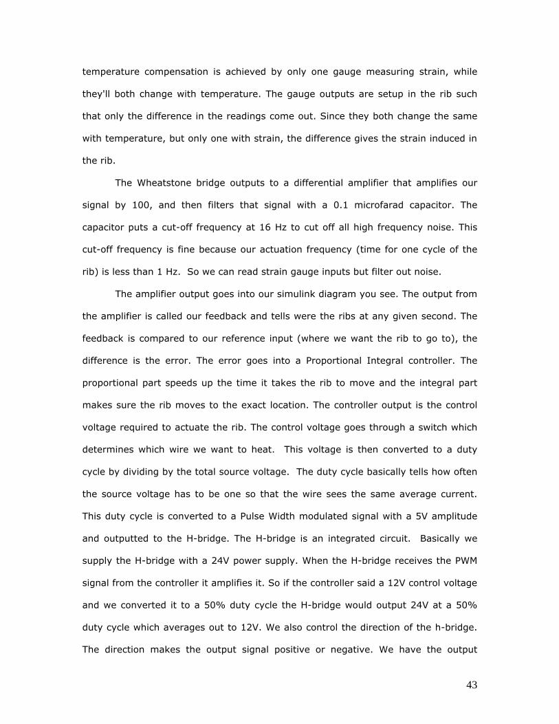
temperature compensation is achieved by only one gauge measuring strain, while

they'll both change with temperature. The gauge outputs are setup in the rib such

that only the difference in the readings come out. Since they both change the same

with temperature, but only one with strain, the difference gives the strain induced in

the rib.

The Wheatstone bridge outputs to a differential amplifier that amplifies our

signal by 100, and then filters that signal with a 0.1 microfarad capacitor. The

capacitor puts a cut-off frequency at 16 Hz to cut off all high frequency noise. This

cut-off frequency is fine because our actuation frequency (time for one cycle of the

rib) is less than 1 Hz. So we can read strain gauge inputs but filter out noise.

The amplifier output goes into our simulink diagram you see. The output from

the amplifier is called our feedback and tells were the ribs at any given second. The

feedback is compared to our reference input (where we want the rib to go to), the

difference is the error. The error goes into a Proportional Integral controller. The

proportional part speeds up the time it takes the rib to move and the integral part

makes sure the rib moves to the exact location. The controller output is the control

voltage required to actuate the rib. The control voltage goes through a switch which

determines which wire we want to heat. This voltage is then converted to a duty

cycle by dividing by the total source voltage. The duty cycle basically tells how often

the source voltage has to be one so that the wire sees the same average current.

This duty cycle is converted to a Pulse Width modulated signal with a 5V amplitude

and outputted to the H-bridge. The H-bridge is an integrated circuit. Basically we

supply the H-bridge with a 24V power supply. When the H-bridge receives the PWM

signal from the controller it amplifies it. So if the controller said a 12V control voltage

and we converted it to a 50% duty cycle the H-bridge would output 24V at a 50%

duty cycle which averages out to 12V. We also control the direction of the h-bridge.

The direction makes the output signal positive or negative. We have the output

44

attached to diodes in opposite direction. Diodes only allow current flow in one

direction so if the input voltage is positive it will go through one diode and heat the

top wire, if the input is negative it will go through the other diode and heat the

bottom wire.

The H-bridges and diodes all source a maximum of 3 amps, which is why we

built the electronics board. 6 H-bridges means 18 amps maximum going through the

system. But it doesn't source 3 amps continually. It sources 3 amps first to get a fast

response but then it settles out oscillating around a 1/4 of an amp to maintain its

position. A very expensive program called D-Space was used to deflect our ribs to

the desired amount, seen in figure 4.12.

Figure 4.12. Visualization of the D-Space program used to actuate ribs.

45

Once the controls were completed, the construction of the plane needed to be

finished. The ribs were then wired with Nitinol, securing the wire to the spar. With these

electronics on board the aircraft, a cowling was needed. This was done by creating a

mold out of Styrofoam by using a band saw and then sanding it into the desired shape and

size. The cowling mold was covered with plastic wrap to ensure a smooth surface and to

keep it intact in case another had to be made. A layer of fiberglass was applied and

shaped appropriately. Once it was formed as desired, the resin was mixed and spread

uniformly onto the mold. After it was dry, the new cowling was removed and trimmed to

fit the center of the aircraft as was needed. The cowling would be attached to the aircraft

by use of Velcro, to make the electronics easily accessible.

To be able to mount this model in the wind tunnel, fiberglass squared can be

attached to the top and the bottom of the plane. The desired location to mount the aircraft

was found by using X-Foil to find the center of gravity. This was found to be 9.85in

from the leading edge. The top mount support should be mounted under the cowling so

that it is not located in the freestream flow. Holes were predrilled in order to securely

and quickly bolt the plane to the mount in the tunnel.

In order to cut the foam in the shape of our airfoil we cut out templates to ensure

that the result of the wings were acceptable. We cut out our leading and trailing edge

foam in the aero bay in the Ware Lab. The tools here were much more suitable to get this

task done, especially their foam cutting bow. The leading edge was made from high

density foam; low density foam was used for the morphing section of the trailing edge.

The leading edge foam was hollowed out so that it could fit over the front of the spar.

The trailing edge was cut so that it would fit over the ribs and was attached to the aircraft

46

using spray epoxy. The skin covers the entire plane to ensure that there is a continuous

surface. It was determined that the skin should be made of very thin latex. This was

chosen because of its light weight and flexibility.

The cost of this aircraft was relatively low. The Nitinol wiring was only $75 for a

spool of 10 meters, and only about half of that was used. The Plexiglas was about $25

for the sheets used. The birch plywood spar cost us about $30 for a 4’ by 8’ sheet. The

foam used rounded to around $50. The electronics totaled to be approximately $100 to

$200. Most of the electronics were acquired from the CIMSS lab. Along with all the

various parts, this aircraft cost nearly $400. This number is lower than the expected

value predicted earlier in the year.

47

Section 4.3 Piezoelectric (PZT) Materials The term piezoelectric refers to a class of natural crystals in which piezoelectric

effects, electricity from applied stress, occur. The first connection made between the

piezoelectric phenomena and a crystalline structure was published in 1880 by Pierre and

Jacques Curie. The term piezoelectricity was applied to this science at that time, to

separate it from other rising scientific technologies, “contact electricity” and

“pyroelectricity”. Since that time piezoelectric materials have been put into service in a

wide variety of applications, from micro/hydrophones, ignition systems, and sonar

systems (Reference 14). Notice that all of these applications reside around one basic

design concept, either sending or receiving small vibrations. Until recently all

piezoelectric material applications were only capable of very small displacements. In

1996 FACE International was granted a field-of-use license to research, produce, and sell

a class of piezoelectric actuators that are based on technology patented by NASA. Those

actuators are known as THin Layer Composite UNimorph Ferroelectric Driver and

SEnsoR (THUNDER). Figure 4.13 shows the construction of a THUNDER actuator.

Figure 4.13. Basic Construction of a THUNDER Actuator. http://www.face-int.com/thunder/thunder.htm

48

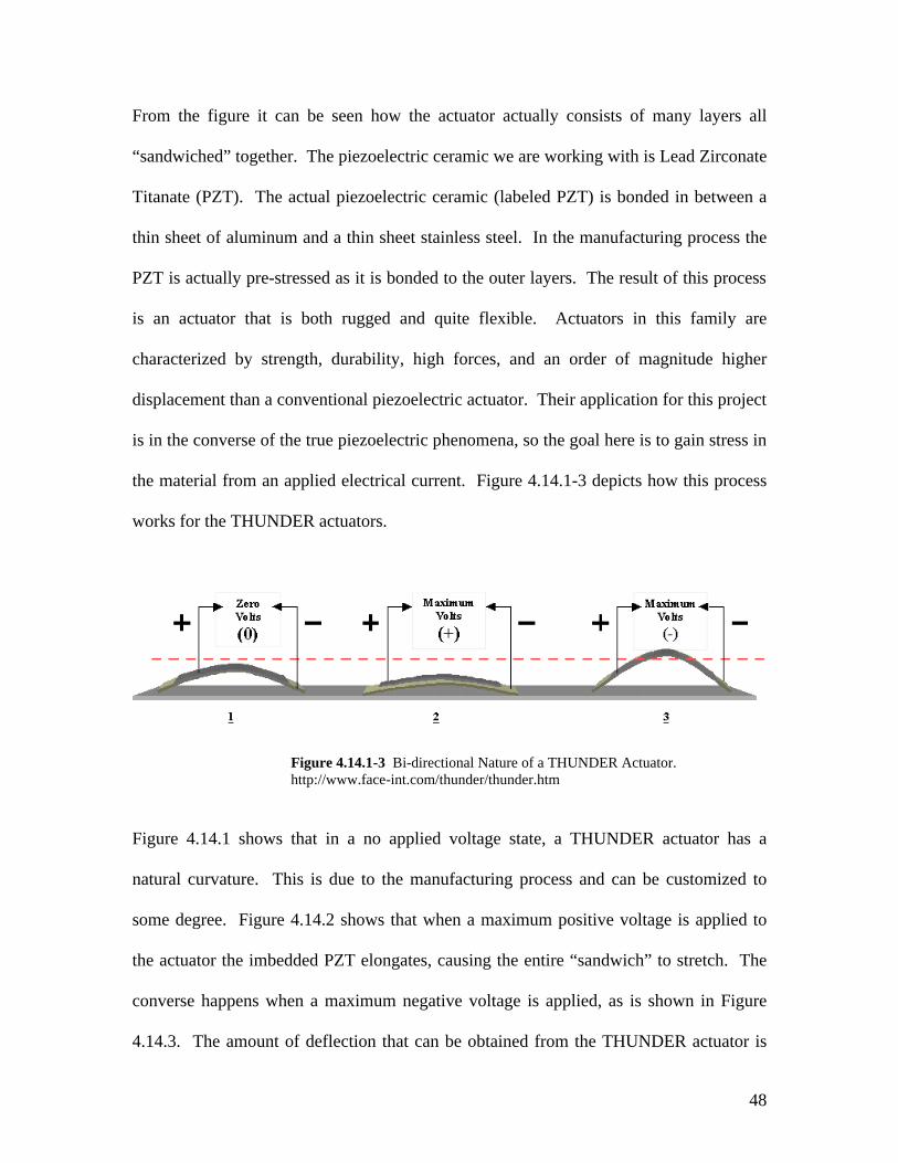
From the figure it can be seen how the actuator actually consists of many layers all

“sandwiched” together. The piezoelectric ceramic we are working with is Lead Zirconate

Titanate (PZT). The actual piezoelectric ceramic (labeled PZT) is bonded in between a

thin sheet of aluminum and a thin sheet stainless steel. In the manufacturing process the

PZT is actually pre-stressed as it is bonded to the outer layers. The result of this process

is an actuator that is both rugged and quite flexible. Actuators in this family are

characterized by strength, durability, high forces, and an order of magnitude higher

displacement than a conventional piezoelectric actuator. Their application for this project

is in the converse of the true piezoelectric phenomena, so the goal here is to gain stress in

the material from an applied electrical current. Figure 4.14.1-3 depicts how this process

works for the THUNDER actuators.

Figure 4.14.1-3 Bi-directional Nature of a THUNDER Actuator. http://www.face-int.com/thunder/thunder.htm

Figure 4.14.1 shows that in a no applied voltage state, a THUNDER actuator has a

natural curvature. This is due to the manufacturing process and can be customized to

some degree. Figure 4.14.2 shows that when a maximum positive voltage is applied to

the actuator the imbedded PZT elongates, causing the entire “sandwich” to stretch. The

converse happens when a maximum negative voltage is applied, as is shown in Figure

4.14.3. The amount of deflection that can be obtained from the THUNDER actuator is

49

proportional to the voltage (positive or negative) applied. Thus, a maximum voltage will

achieve as much of a displacement as is possible, and as the voltage applied decreases, so

does the displacement (Reference 15). The voltage range of the Thunder PZT is from

minus 298 to 595V. The displacement versus voltage for these actuators is repeatable

and nearly linear. A certain displacement will be obtained from a known applied voltage.

The motion of the actuator is dependent on the signal type. If a DC voltage is applied,

the PZT will hold that displacement until the voltage is changed; if a sine wave is

applied, the motion of the PZT will follow the sine wave voltage. The predictability and

linearity of the Thunder actuators allows us to incorporate them into a reliable open-loop

control system.

To achieve a maximum tip deflection with the THUNDER actuators they have to

be mounted in a cantilevered fashion. That means that one end of the actuator is

constrained while the other is allowed to “float”. With it set in a cantilevered position,

the tip displacement ranges from -0.15 to 0.30 in. This is the ideal situation when the

PZTs are being considered as the method of actuating a camber change at individual

stations along the span. Figure 4.15 is a conceptual drawing of a model that would use

PZTs mounted in a cantilevered fashion to achieve independent control deflections along

the span.

50

Figure 4.15. Conceptual Drawing of a Morphing Wing Aircraft with PZT

Actuators.

In Figure 4.15 the black structure is the wing box which is projected to be

manufactured out of a composite material. The blue/green structure represents the

leading and trailing edge sections which would be actuated by the PZTs, which are the

grey objects drawn between the wing box and the leading/trailing edge sections. The

leading and trailing edge sections will have to be flexible enough so as to allow the PZTs

to bend and twist them to produce the required camber change. Thus, the material of

choice for those sections would be a light weight and flexible foam. The cowling at the

centerline of the model (shown in Figure 4.15 as maroon) would house all of the onboard

electronics and fuel tanks.

The benefits of using PZTs are that they are lightweight and have an almost

instantaneous response time once a voltage has been applied. Both of which are very

desirable characteristics of an actuator for an aircraft control surface. Despite that, the

51

disadvantages of PZTs are quite significant. First, is that PZTs are very cost prohibitive.

Each THUNDER actuator is hand made to each customer’s specifications. This of course

makes them very expensive, between $80 and $100 each. On top of that, it has been

estimated that at least 10 THUNDER actuators would be required to achieve the

necessary control deflections. Thus, an aircraft relying totally on PZTs would be very

expensive. Next is their power requirement. The “maximum voltage” required to obtain

their maximum displacement is on the order of 600 volts. It has been estimated that

voltages on that magnitude will not be required to obtain the necessary control

deflections. However, the voltages required will still probably quite higher than the

average battery pack could supply. Thus, a fully functional model aircraft controlled

solely by PZTs would require a very specialized power supply to fly.

PZT Final Design

A primary design concern of the concept presented in Figure 4.14 was whether or

not the PZTs would be able to maintain the airfoil geometry around the leading edge

where the pressure gradient is the strongest. Thus, the PZTs actuating the leading edge

would be required to first constantly sustain the basic aerodynamic loading and then

overcome that aerodynamic loading when a control deflection was scheduled. It was felt

that the voltage requirements necessary to deflect just the trailing edge of the aircraft

were significant enough. Thus, to require further voltage increases to include leading

edge actuation would substantially decrease the PZT plane’s chances of free flight.

Therefore, the concept shown in Figure 4.15 was redesigned to the final concept shown in

Figure 4.16.

52

Figure 4.16. A physical layout of the PZT actuated morphing plane.

The final PZT design was constructed of a high-density foam core. The front

portion of the plane was foam wrapped in two layers of rigid fiberglass/epoxy composite,

while the trailing edge of each wing was simply one continuous section of foam, as

shown in Figure 4.16. Each wing has four Thunder TH-7R PZT actuators distributed

equally along the span. The actuators are the only link between the rigid leading

edge/wing box and the flexible trailing edge, which allowed for continuous morphing of

the trailing edge at different span wise locations. A flexible skin was placed over the

wing section containing the PZTs in order to maintain the airfoil geometry in these

sections. A hollow, rigid fiberglass cowling was attached to the fuselage portion of the

aircraft in order to house the control circuitry. The rigid portion aft of the fuselage is

53

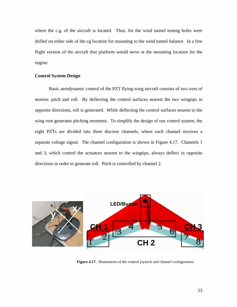
where the c.g. of the aircraft is located. Thus, for the wind tunnel testing holes were

drilled on either side of the cg location for mounting to the wind tunnel balance. In a free

flight version of the aircraft that platform would serve at the mounting location for the

engine.

Control System Design

Basic aerodynamic control of the PZT flying wing aircraft consists of two axes of

motion: pitch and roll. By deflecting the control surfaces nearest the two wingtips in

opposite directions, roll is generated. While deflecting the control surfaces nearest to the

wing root generates pitching moments. To simplify the design of our control system, the

eight PZTs are divided into three discrete channels, where each channel receives a

separate voltage signal. The channel configuration is shown in Figure 4.17. Channels 1

and 3, which control the actuators nearest to the wingtips, always deflect in opposite

directions in order to generate roll. Pitch is controlled by channel 2.

Figure 4.17. Illustrations of the control joystick and channel configuration.

1 2 3 5 4 6 7 8 CH 2

CH 1 CH 3

LED/Buzzer

y x

54

The input to the control system comes from a simple 2-axis joystick, with the X-

axis on the joystick controlling roll and the Y-axis controlling pitch. Small joystick

deflections generate small PZT displacements, while maximum joystick deflection along

either axis generates large PZT displacements. Table 4.2 shows actuator voltage for

typical control inputs. The joystick trigger activates an LED in the nose of the plane as

well as a buzzer.

Table 4.2. Actuator voltage for typical control inputs.

The assembly code consisted of three main sections. The first used an A/D routine

to sample the current variable resistor values. Then those values were used to generate

three separate PWM signals. Finally, the trigger was checked and the LED/buzzer

activated or deactivated. The pitch potentiometer of the joystick controlled the center

PZT bank directly. This worked because the PZTs need to be partially excited for level

flight and the joystick variable resistors gave a middle value when the joystick was

centered. This meant the analog resistor values could be directly sent to the PWM

routine. The roll resistor on the joystick controlled the outer two PZT banks. One bank

got the direct analog value and the other got the inverse. This created the roll desired

when using the joystick.

The PWM routine decremented a counter from 255 to 0. When it started the three

PWM signals go low or high and when the counter reached the analog value from the

Required Actuator Voltage Input Joystick Input 1 2 3 4 5 6 7 8

Roll Left 0 0 50% 50% 50% 50% 100% 100% Roll Right 100% 100% 50% 50% 50% 50% 0 0 Pitch Up 50% 50% 100% 100% 100% 100% 50% 50%

Pitch Down 50% 50% 0 0 0 0 50% 50%

55

joystick it toggled the appropriate PZT bank. Each PWM had the same period, but the

duty cycles were all independent. One period was generated and then the program

continued. The PIC cycled fast enough so that it outputs three separate and variable

PWMs on its output pins.

Three banks of PZTs needed to be controlled; each separately excited with a

range of 0 – 600 V. The design approach was to control the PZTs in the same fashion as a

motor speed controller. The two variable resistors in the analog joystick were used to

provide the control signals for the PZTs. The H-bridge could not, however, be used due

to the high voltages being switched. Instead, a HEXFET was used to switch the PZT

from 0 to 600 volts. A HEXFET is a type of MOSFET, which can be fully turned on at 5

volts. Because it is a voltage-controlled device the VT84 can directly switch the

HEXFET and thus control the PZT.

A PZT does not have the inertia to average the PWM signal output by the VT84.

If given a square wave directly the PZT will respond to all the voltage oscillations. A

smoothing filter (30k resistor and 470uF capacitor) was used to average the PWM signal

on the high side of the MOSFET. By using a fairly large capacitor and a high frequency

PWM, the PZT reacted as if it were getting a steady DC value. Also, because a PZT is

essentially a capacitor, a 430k resistor was used to provide a route for it to discharge

when the MOSFET was turned off. If this resistor were omitted, the PZT would react

slowly when the voltage to it was turned off. This circuit can be seen in Figure 4.18.

56

Figure 4.18. Illustrations of the circuit designs.

As an extra part of the project, the trigger on the joystick was used to activate a

LED/buzzer on the plane. The trigger was connected to an input pin on the VT84 and the

LED/buzzer were connected to an output pin. These circuits can also be seen in Figure

4.18.

x3

Trigger

57

Section 5. Testing of the Zagi 400x.

To obtain baseline data of a model RC flying wing, a Zagi Model 400x was

purchased. The geometry of the Zagi was modeled using a Vortex Lattice Method

(VLM) code in order to obtain estimates of the model’s performance. Then, the model

was tested in the Virginia Tech Stability Wind Tunnel. The results of the VLM code and

the wind tunnel testing are presented below.

Section 5.1. Aerodynamic Analysis of the Zagi 400x using the VLM 4998

FORTRAN Code

The VLM 4998 FORTRAN code was applied to the Zagi 400x in order to validate

the wind tunnel results and show that a vortex lattice method could be used to accurately

predict the aerodynamic characteristics of a small scale, low Reynolds number aircraft.

The most important information required from the VLM code for design purposes was

the CM0L, CLMAX, CMα, and CLα. The effect of control deflections on the CM0L and CLMAX

were also of great importance because a flying wing was being considered.

The input information required by the code included the following: the x, y

location of the break points, dihedral at each break point, angle of attack of the mean

camber line at each control point, and center of gravity. The code also required the user

to specify the number of horseshoe vortices along the span and chord. Seven chordwise

horseshoe vortices were chosen so that the hinge-line of the elevons lay near the front

edge of a spanwise row of vortices. The angle of attack of the mean camber line at each

control point was found by estimating the airfoil shape and obtaining its coordinates. A

polynomial was fit to the mean camber line of the airfoil coordinates. Assuming small

angles, the derivative of the mean camber line polynomial allowed the angle of attack at

58

each control point to be computed. To model the washout of the Zagi, a linear variation

of two degrees from root to tip was subtracted from the angle of attack at each control

point. This was later found to be a mistake because a straight line wrap does not result in

a linear twist distribution. But this would not affect the results significantly because as

can be seen in the “Design Considerations” section of this report, a straight line wrap

twist distribution is not significantly different from a linear distribution. Elevon

deflections were modeled by adding the elevon deflection angle to the angle of attacks of

the trailing edge control points.

Fig. 5.1 compares the CL-alpha curve computed from the VLM code to that

measured in the wind tunnel for three different elevon deflections.

Fig. 5.1 shows that the VLM prediction fit well for the no deflection case, but did

not come close for the deflected elevon cases. The same trend is seen in the CL-CM

Fig. 5.1 Comparison of VLM and Wind Tunnel Results

-2

-1.5

-1

-0.5

0

0.5

1

1.5

2

2.5

-10 -5 0 5 10 15 20 25

AOA (degrees)

CL

No Deflection (VLM)+20 deg (VLM)-20 deg (VLM) No Deflection (WT)+20 deg (WT)-20 deg (WT)

59

comparison shown in Fig. 5.2. The main problem with the VLM’s predictions was the

zero-lift angle of attack, which is responsible for the large offsets of the deflected elevon

curves with respect to the wind tunnel data.

The VLM’s inability to predict the zero-lift angle of attack for deflected elevon

cases was because the vortex lattice method is an inviscid analysis. Because the Zagi was

tested at relatively low Reynolds number (38,000), the flow remained mostly laminar,

and flow separation likely occurred at very low angles of attack (it should be noted that

tufts were later added to observe separation, but were assumed to cause transition early).

This would have severely affected the elevons’ effectiveness, and the resulting lift and

pitching moments. For the downward elevon deflection, the flow likely separated off the

top of the elevon therefore decreasing the wing’s lift and negative pitching from that

predicted by the VLM’s inviscid analysis. For the upward deflection, flow separation

likely occurred on the bottom side of the elevon causing an increase in the lift and

Fig. 5.2 Comparison of VLM and Wind Tunnel Results

-2

-1.5

-1

-0.5

0

0.5

1

1.5

2

2.5

-0.5 -0.4 -0.3 -0.2 -0.1 0 0.1 0.2 0.3 0.4 0.5

CM

CL

No Deflection (VLM)+20 deg (VLM)-20 deg (VLM) No Deflection (WT)+20 deg (WT)-20 deg (WT)

60

pitching moment from that predicted by the VLM code. It is important to point out that

the flow visualization performed on the Zagi using tufts did not show any obvious flow

separation over the deflected elevons with the Zagi at low angles of attack. But, this is

likely due to the presence of the tufts, which “tripped” the flow, causing transition early

and allowing the flow to stay attached over the elevons. If further wind tunnel tests were

conducted on the Zagi, the effect of transition on the elevon effectiveness could be

examined by performing tests that forced transition to occur in front of the elevons.

The VLM analysis proved to be effective in predicting the aerodynamic

characteristics of the Zagi with no elevon deflections, which makes it acceptable for the

use in the preliminary stages of our morphing wing design. But it was very cumbersome

to use, especially for analyzing control deflections. This led to the development of the

vortex lattice code mentioned in the previous section and discussed in Appendix 1.

Section 5.2 Wind Tunnel Testing of the Zagi 400x

Before developing a full-scale model of our morphing concepts, it was desired to

acquire a set of data that we could use as realistic values to base some of our initial

calculations on. Since the full-scale vehicle will have a wingspan between 48 and 55

inches, moment and coefficient plots and control sizes from a commercial or military jet

would not be any help as a reference. Another reason for developing a “small-scale”

database is that the full-scale morphing aircraft will be operating at relatively low

Reynold’s numbers, where there has not been extensive testing relating to this design.

The Zagi 400X made by Zagi Inc. was chosen as the test vehicle since it is a

commercially proven design and fits in the Virginia Tech Stability Tunnel. The 400X is

61

a high-performance aerobatic flying wing. The 400X is radio controlled and uses an

electric motor with a pusher prop. The model has flexible winglets that provide yaw

stabilization and full-span elevons. The geometry of the Zagi 400X is shown below.

Table 5.1

b 48.00" Cr 13.00” Ct 6.75” ? 0.519 LLE 30.570

Wind tunnel testing was performed in the Virginia Tech Stability Tunnel with the

SB-1 balance shown below in Figure 5.3. The balance has internal strain gauges that

measure the forces and moments on the model.

Figure 5.3 SB-1 Balance Used for Wind Tunnel Testing.

The test balance moves the model through angles of attack of –6 to 20 degrees.

To prepare the model for testing, a mount was fabricated from high-density fiberglass

plates. Each piece was the same shape as the mounting surface of the balance, with holes

drilled at each corner. One plate was placed on the top and bottom surface of the 400X,

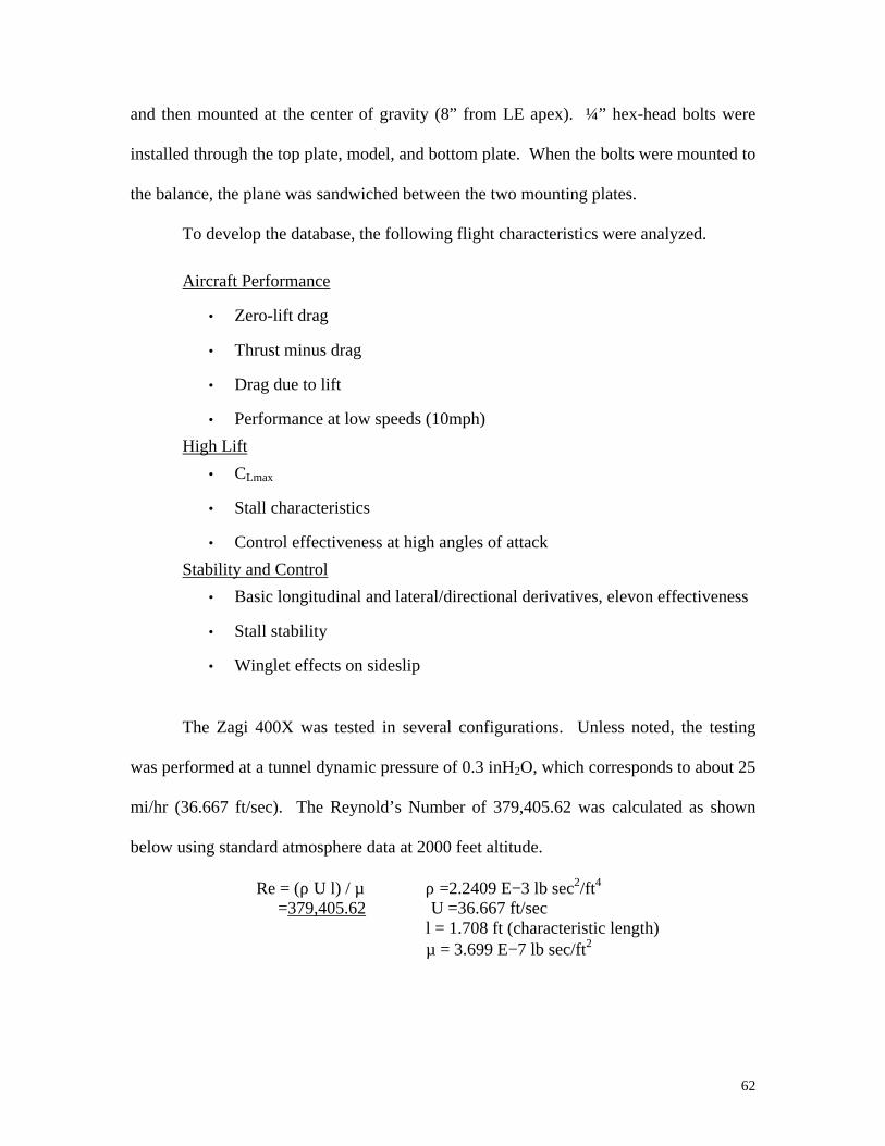
62

and then mounted at the center of gravity (8” from LE apex). ¼” hex-head bolts were

installed through the top plate, model, and bottom plate. When the bolts were mounted to

the balance, the plane was sandwiched between the two mounting plates.

To develop the database, the following flight characteristics were analyzed.

Aircraft Performance

• Zero-lift drag

• Thrust minus drag

• Drag due to lift

• Performance at low speeds (10mph)

High Lift

• CLmax

• Stall characteristics

• Control effectiveness at high angles of attack

Stability and Control

• Basic longitudinal and lateral/directional derivatives, elevon effectiveness

• Stall stability

• Winglet effects on sideslip

The Zagi 400X was tested in several configurations. Unless noted, the testing

was performed at a tunnel dynamic pressure of 0.3 inH2O, which corresponds to about 25

mi/hr (36.667 ft/sec). The Reynold’s Number of 379,405.62 was calculated as shown

below using standard atmosphere data at 2000 feet altitude.

Re = (ρ U l) / µ ρ =2.2409 Ε−3 lb sec2/ft4 =379,405.62 U =36.667 ft/sec

l = 1.708 ft (characteristic length) µ = 3.699 Ε−7 lb sec/ft2

63

First, a tare run was performed as a “zero” for the following tests. The control

effectiveness was tested in pitch and roll by deflecting the elevons +10 and +20 degrees

in each mode. Next, a test was done with no deflection and without the winglets in order

to study the winglet contributions in straight and level flight. With the winglets off, the

balance was rotated 11.5 degrees clockwise and tested in the angles of attack. The model

was also tested at the 11.5o sideslip angle with the winglets on so that the winglet

effectiveness could be studied. The model was then fitted with tufts and rotated back to

zero sideslip for a flow visualization test. The flow visualization showed that the flow

separation creeps slowly forward until a predictable stall around 12 degrees AoA. The

stall point remained around 12 degrees in all the tests. The model was also tested at a

tunnel dynamic pressure of 0.1 inH2O (10 mi/hr) with zero deflection. This run was to

test the model’s performance in low speeds, which is important when landing. The lower

speed caused the 400X to stall at 10 degrees AoA with a 13% lower CLmax . Figures 5.4

and 5.5 show the Zagi 400X before and during testing. The results and discussion of the

tunnel testing are presented below.

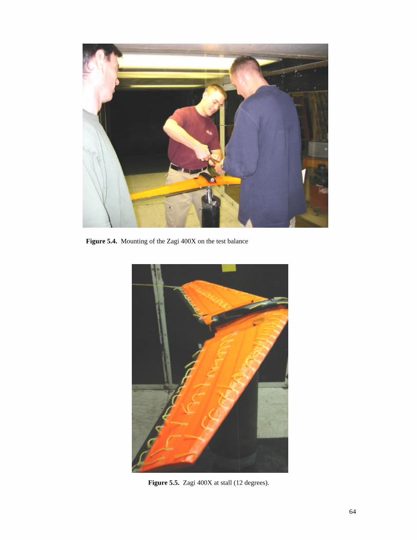
64

Figure 5.4. Mounting of the Zagi 400X on the test balance

Figure 5.5. Zagi 400X at stall (12 degrees).

65

Section 5.3. Results of ZAGI 400x Wind Tunnel Testing.

By testing our baseline model we learned several things about this aircraft. By

looking at the most basic plot (Fig 5.6) showing the CLα curve you can see that the Zagi

400X stalls at an angle of attack of 12°. For analysis “negative deflection” corresponds

to a nose-down pitching moment, and “positive deflection” a nose-up moment. By

causing negative elevon deflection, lift was increased. Positive deflection corresponded

to a decrease in lift. CLmax for zero deflection is 0.9541. By using elevon deflection, the

CLmax was 1.1776 for negative deflection and 0.6842 for positive deflection. Knowing

the stall location and how much the deflection of the elevons affects the lift will help us

in designing our final aircraft.

Figure 5.6. Effects of elevon deflection on the lift coeficient

-0.60

-0.40

-0.20

0.00

0.20

0.40

0.60

0.80

1.00

1.20

1.40

-10.00 -5.00 0.00 5.00 10.00 15.00 20.00 25.00

AoA (deg)

Cl

Zero deflection +10 deg +20 deg -10 deg -20 deg

No elevon deflection

Increasing elevon deflection

Decreasing elevon deflection

Clmax (stall)

66

The pitching moment coefficient versus the angle of attack plot (Fig 5.7) verifies

this as a stable aircraft. For the zero deflection and negative deflection runs, the data

shows that the aircraft has a tendency to nose down; a characteristic of aircraft stability.

This self-righting ability allows an aircraft to recover from a stall by decreasing angle of

attack and lowering the CL. For the +10 degree run for most of the positive angles of

attack it is also stable. It is unstable for +20 degree before 16° angle of attack. The trend

of decreasing Cm is correct.

The best technique to find CL and CD at minimum drag is to plot them versus each

other and graphically determine this point, see figure 5.8. This location is where a line

from the origin tangent to the curve (zero deflection) intersects. At this point is the

Figure 5.7. Effects of elevon deflection on the pitching moment coeficient

-0.25

-0.20

-0.15

-0.10

-0.05

0.00

0.05

0.10

0.15

0.20

0.25

-10.00 -5.00 0.00 5.00 10.00 15.00 20.00 25.00

AoA (deg)

Cm

Zero deflection +10 deg +20 deg -10 deg -20 deg

No elevon deflection

Increasing elevon deflection

Decreasing elevon deflection

Stall

67

location for minimum drag. At the specified test conditions, the Zagi 400X had its

CLmindrag is 0.71 and the CD min drag is 0.035. In Figure 5.8, the curve for +10 degrees of

deflection it can be seen that the curve goes into the realm of having a negative drag

coefficient. This could be interpreted as the Zagi generating thrust as it is sitting in the

wind tunnel. Of course this is not the case. That data sweep is bogus and thus ignored in

the determination of the minimum drag CL and CD.

Figure 5.8. Cl vs Cd

-0.60

-0.40

-0.20

0.00

0.20

0.40

0.60

0.80

1.00

1.20

1.40

-0.050 0.000 0.050 0.100 0.150 0.200 0.250 0.300 0.350 0.400 0.450

Cd

Cl

Zero deflection +10 deg +20 deg -10 deg -20 deg

Min Drag

Deflecting one elevon up and the other down creates roll moments. Due to port-

starboard symmetry, the rolling moment in one direction is taken as equal to the other.

The resulting roll coefficients were plotted versus the angle of attack in figure 5.9. The

68

roll coefficient increases with roll deflection, as it should. However, the plot showing

zero deflection looks slightly erratic and is not equal to zero as it should be. This is due

to the lack of precision of setting up the elevon positions. This was done by moving the

control surfaces to the desired positions. There may also be asymmetries in the aircraft

after construction. If the mount wasn’t fitted tightly enough, this could have resulted in

unwanted roll and would disturb our results.

To study yaw affects on the Zagi the mount was rotated 11.5° clockwise to

establish an initial yaw (figure 5.10). The model had a slight increase in the yawing

coefficient when it was set up to run straight. This should be zero, but due to

asymmetries in the model we could not prevent this from occurring. By causing the side

-0.14

-0.12

-0.10

-0.08

-0.06

-0.04

-0.02

0.00

0.02

0.04

0.06

0.08

0.10

-10.00 -5.00 0.00 5.00 10.00 15.00 20.00 25.00

AoA (deg)

CL

Zero deflection 10 deg Roll 20 deg Roll

Increasing Roll Deflection

Figure 5.9. Roll coefficient vs AOA

Not zero due to asymmetries andlack of precise test methods

69

slip, the aircraft is undergoing a yawing moment. By removing the winglets at this

configuration, we can test their effectiveness. The yawing moment without the winglets

is half as strong as the aircraft with the winglets. This tells us that the winglets are

effective in creating a yawing moment that will straighten out the aircraft, making it more

stable around that axis.

By decreasing the dynamic pressure (Q) in the wind tunnel, essentially decreasing

the velocity, we can see the effect on stall. At a Q of 0.1in H2O, corresponding to about

10mph, the stall location drops to an angle of attack of 10° as seen in figure 5.11 below.

This is a 13% lower CLmax than at 25mph. This decrease in stall location makes sense

Figure 5.10. Effects of varying sideslip on the directional stability coefficient

-0.014

-0.012

-0.01

-0.008

-0.006

-0.004

-0.002

0

0.002

0.004

0.006

0.008

-10 -5 0 5 10 15 20 25

AoA

Cn

Phi = 0 (winglets) Phi = 11.5 (winglets) Phi = 11.5 (no winglets)

IncreasingSide Slip

No Winglets

Winglet

70

because we are also lowering the Reynolds Number from approximately 400,000 to

150,000.

Knowing this information about our baseline model will help us in designing our

morphing model. Because we are basing our aircraft on the Zagi, we can use this to our

advantage. Knowing the stall location, minimum drag information, roll effectiveness,

and sideslip affects before we design our own aircraft will prove to be very beneficial.

We can use this pre-designed model to our advantage by allowing us to know what

aspects of this aircraft we can use on our own model and what we need to improve so that

our morphing design aspects will be fully utilized.

Figure 5.11. Testing at 10mph, zero deflection

0

0.1

0.2

0.3

0.4

0.5

0.6

0.7

0.8

0.9

-10 -5 0 5 10 15 20 25

AoA

Lif

t C

oef

fici

ent

Clmax

71

Section 6. Design Testing. To test the aerodynamic effects of morphing and to validate the morphing

concepts predicted by the morphing specific VLM code, the PZT and servo models were

tested in the Virginia Tech Stability Tunnel. The SMA model faced complications in the

control system and could not be finished in time for testing. The PZT control system also

experienced difficulties but the model was still tested. Due to an insufficient refresh rate

in the PIC microprocessor, the PZT model was only tested with uniform trailing edge

deflections. The result of uniform deflections is that the model cannot be trimmed for

maximum efficiency in various modes of flight. The data from the PZT model’s testing

was used as a comparison to the servo’s morphed configurations. The servo model was

tested with the morphing capabilities desired in the design of the model. Wind tunnel

testing occurred on 26-28 April 2002. The standard dynamic pressure during testing was

Q = 0.50 inches of water.

Test Equipment and Facility

The testing was conducted in the Virginia Tech 6’ x 6’ Stability Tunnel on the

SR-1 Strut Mount/Strain Gauge Balance. The load limit data for this balance are shown

in Table 6.1

72

Table 6.1. Standard tunnel balance limits.

SR-1 (Strut Mount)

Normal Force [lb] 200 Axial Force [lb] 100

Side Force [lb] 100

Pitching Moment [in-lb] 200

Rolling Moment [in-lb] 300 Yawing Moment [in-lb] 200

http://www.aoe.vt.edu/aoe/physical/tunnel_inst.htm

The balance outputs the forces, pressures and temperatures to the tunnel's data

acquisition system. The centerpiece of the system is an SCXI-1001 Mainframe from

National Instruments. The isolation and amplification of 8 differential analog voltages

has an input range of -10 to +10 volts. The inputs are read by a National Instruments AT-

MIO-16-XE-10 Data Acquisition Card installed in a Pentium 133 computer. This results

in a total of 32 isolated differential analog input channels with an Analog to Digital

conversion resolution of 16 Bits. All of the software for data acquisition is written using

Lab View 4.0 under the Windows 95 environment. Collected data can be stored on the

computer hard drive, and then transferred to writeable Compact Disc, Zip Disk, sent over

the Internet, or transferred over the Aerospace network. The entire data acquisition

system is shown in Figure 6.1.

73

Figure 6.1. Data acquisition system, showing control computer and electronics rack. http://www.aoe.vt.edu/aoe/physical/tunnel_inst.htm

Section 6.1. Comparison between the PZT and Servo Results. Because the PZT and Servo models were built to different scales with different

materials, it was important to get baseline data for each model to serve as a correction

factor so that the servo model’s independent spanwise actuation could be compared to the

PZT’s one-piece elevon. This was done by testing each model in an undeflected

configuration through an entire –6 to 18-degree alpha sweep. It is important to note that

the PZT model’s planform was built to a 10% smaller scale than the servo model. The

PZT model also used a 9% thick airfoil as opposed to the Servo model’s 12% thick

airfoil. The wind tunnel dynamic pressure was adjusted accordingly to maintain a

constant Reynolds number for the two models.

74

Figure 6.2 shows the CL - α plot for each aircraft in the undeflected state. It is

seen that the servo model had an approximately 2.5-degree lower zero-lift angle of attack

than the PZT model. The vortex lattice method predicts a –5-degree zero-lift angle of

attack, which agrees well with the servo model. The stall angle of attack for the servo

model is shown to be about 2-degrees greater than that for the PZT model. The PZT’s

thinner airfoil sections most likely caused this, but it could also have been a result of

aeroelastic deformations. It should be noted that the servo model had 12 independent ribs

to be controlled, and it is possible that the deflections were not exactly zero when these

tests were run.

Figure 6.3 shows the CL – CD plot for both models. Again, there appears to be a

considerable difference between the two models. Most apparent is the PZT’s lower drag

for a given CL, until its CLmax was reached, than the Servo model. This is a consequence

of the PZT model’s thinner airfoil sections.

75

Figure 6.2. Wind Tunnel Data Comparison Between the Servo and PZT Aircraft.

Figure 6.3. Wind Tunnel Data Comparison Between the Servo and PZT Aircraft.

-0.40

-0.20

0.00

0.20

0.40

0.60

0.80

1.00

-10.0 -5.0 0.0 5.0 10.0 15.0 20.0

Angle of Attack (deg)

CL

Servo

PZT

-0.40

-0.20

0.00

0.20

0.40

0.60

0.80

1.00

0.00 0.05 0.10 0.15 0.20

CD

CL

Servo

PZT

76

Figure 6.4 shows the CL - CM plot for each model. This plot is somewhat

disturbing because it shows that both models were producing a positive CM0L in an

undeflected configuration. Vortex lattice predicted a CM0L of –0.015 with 4-degrees of

washout present. If it is assumed that the disagreement between theory and the data was

not caused by instrumentation problems, then it must be that the models became

deformed during the tests due to aerodynamic loads. This is conceivable because of the

foam construction of the wings. The servo model did not have a fiberglass cover over the

wing like the PZT model did. The servo model instead used two carbon-fiber spars. The

two spars were placed relatively close to each other because of the size of the control

surfaces. It is also important to note that the leading edge spar was mistakenly placed too

far aft therefore minimizing even more the distance between the spars. It is possible that

aerodynamic loads could have twisted the servo model’s wing causing severe changes in

the pitching moments.

Figure 6.4 Wind Tunnel Data Comparison between the Servo and PZT Aircraft.

-0.01

0.00

0.01

0.02

0.03

0.04

0.05

0.06

0.07

0.08

-0.20 0.00 0.20 0.40 0.60 0.80 1.00

CL

CM

Servo

PZT

77

Section 6.2. Morphing Wind Tunnel Results.

One of the main benefits of morphing is the ability to operate at an off design CL

with a minimal increase in CD. Figure 6.5 is a trimmed CD – CL comparison plot for the

Servo, PZT, and Zagi models. Recall the design CL for both the Servo and PZT models

was 0.3. At the “off design” CL of 0.1 it can be seen that both models experienced an

increase in CD. The PZT model, operating with uniform deflections across the span

experienced a 12% increase in the drag coefficient. The Servo model, which was

operating with the morphed trailing edge ratio schedule (Table 3.2), experienced only a

7% increase in the drag coefficient. Thus, the concept of scheduling trailing edge

deflections in order to obtain minimum drag at a variety of CLs was verified.

Figure 6.5. Drag Dependence on the Trimmed CL.

The other design condition for the morphing wing was the high-lift configuration

presented in Section 3.3. The purpose here was to have a new schedule (Table 3.3) of

deflection ratios that would allow the aircraft to trim at a maximum CL. Figure 6.6 is a

Drag Dependence on the Trimmed CL

0.00

0.01

0.02

0.03

0.04

0.05

0.06

0.00 0.10 0.20 0.30 0.40 0.50CL

CD

Zagi Baseline Model

PZT Model

Servo Model usingMin-Drag Deflections

Data collected from tests in theVirginia Tech Stability Wind Tunnel.

Reynolds Number = 40,000

The drag increase from a change in trimmed CL from 0.3 to 0.1 was 12% for the PZT model, 7% for the Servo Model, and 16% for the Zagi.

78

comparison plot for the trimmed CLmax achieved by the PZT and Servo planes. From this

plot it can be seen that the model operating under the high-lift morphing scheduling (the

Servo model) trimmed out at a considerably higher CL than the model operating with

uniform trailing edge deflections (the PZT model). This again validates the morphing

specific VLM code’s predictions that a morphed trailing edge can out perform a

uniformly deflected trailing edge.

Figure 6.6. Trimmed CLmax Capability of the Morphing Models.

Lmax

-0.01

0.00

0.01

0.02

0.03

0.04

0.05

-0.20 0.00 0.20 0.40 0.60 0.80 1.00

CL

CM

PZT Model

Servo Model using the high-lift deflections.

Servo Trimmed CLmaxPZT Trimmed CLmax

79

Section 7. Project Summary

At the inception of the project, the Virginia Tech Morphing Wing Design Team

set the goal of designing and building small-scale aircraft that demonstrate the

benefits of scheduling actuation of control surfaces. Throughout the course of the

project, three model aircraft were designed and built, each relying on a unique type of

actuator to achieve the desired trailing edge shapes. The actuation methods were

piezoelectric ceramics, shape-memory Nickel Titanium alloy, and conventional

servomotors. A flying wing planform was chosen as the testbed for this project since

any benefits of morphing would most likely be revealed more clearly. Success of the

project was based on the demonstrated aerodynamic improvement of the morphing

models against a commercial flying wing of similar scale that was controlled with

conventional one-piece elevons.

To aid in the design of these models, a morphing specific VLM code

(MorphVLM) was developed to obtain aerodynamic predictions. This code allowed

the theoretical testing of various trailing edge shapes in order to optimize values for a

trimmed CLmax. Wind tunnel testing was conducted to analyze the aerodynamic

characteristics of the morphing and conventional models to isolate the effects of

morphing. After comparing the wind tunnel data, it is concluded that morphing

technologies has great potential for improving the aerodynamics of aircraft. Although

none of the models were flight tested, the improved performance gained through

morphing led to the overall success of the project.

80

REFERENCES 1. Spillman, J.,” The use of variable camber to reduce drag, weight and costs of

transport aircraft,” Aeronautical Journal, January 1992, v 96, pp 1-8. 2. Abott, L. H. and von Doenhoff, A..Z., Theory of Wing Sections, Dover Publications,

New York, 1949. 3. Stanewsky, E., “Adaptive Wing and Flow Control Technology,” Progress in

Aerospace Sciences, v 37, Elsevier Science Ltd., 2001, pp. 583-667. 4. Siclari, M. J. and Austin, F., “Optimization of a Realistic Flap Design for In-Flight

Transonic Performance Enhancement,” AIAA Paper No. 98-0596, presented at the 36th Aerospace Sciences Meeting & Exhibit, Reno, NV, Jan. 1998.

5. Greff, E. “The development and design integration of a variable camber wing for

long/medium range aircraft,” Aeronautical Journal, Nov. 1990, v 94, pp 301-312. 6. Hilbig, H., and Wagner, H., “Variable Wing Camber Control For Civil Transport

Aircraft,” ICAS-84-5.2.1, pp. 243-248, 1984. 7. Renken, J.H., “Mission – Adaptive Wing Camber Control Systems for Transport

Aircraft” AIAA Paper No. 85-5006, presented at the 3rd Applied Aerodynamics Conference, Colorado Springs, CO, October, 1985.

8. Frost, et al., United States Patent No. 4,247,066, “Airfoil Variable Cambering Device

and Method.” General Dynamics Corporation, Fort Worth, TX, February 21, 1978. 9. Statkus, Frank D., United States Patent No. 4,351,502, ”Continuous Skin Variable

Camber Airfoil Edge Actuating Mechanism.” The Boeing Company, Seattle, WA, May 21, 1980.

10. Ball, W.H., Ishimitsu, K.K., United States Patent No. 4,012,013, “Variable Camber

Inlet for Supersonic Aircraft.” The Boeing Company, Seattle, WA, February 5, 1976 11. DeCamp, R.W., Hardy, R., “Mission Adaptive Wing Advanced Research Concepts”,

AIAA Paper No. 84-2088, August 1984. 12. Smith, S.B., Nelson, D.W., “Determination of the Aerodynamic Characteristics of the

Mission Adaptive Wing”, AIAA Paper No. 88-2556, presented at the 6th Applied Aerodynamics Conference, Williamsburg, VA, April 29, 1989.

13. Baer-Riedhart, J. “Active Aeroelastic Flight Research, ‘Back to the Future’”. NASA

Document No. 2002-03-061 DFRC, March 2002.

81

14. Piezo Systems, “History of Piezoelectricity”, 1994, last accessed 22 April 2002, http://www.piezo.com/history.html

15. FACE International Corporation, “THUNDER Actuators”, 1998, last accessed 22

April 2002, http://www.face-int.com/thunder/tech/ttech.htm 16. Heperle, Martin, “MH 45”, 2001, last accessed 23 April 2002,

http://beadec1.ea.bs.dlr.de/Airfoils/mh45koo.htm

Appendix 1. The MH-45 Airfoil

The MH-45 airfoil, shown in Fig. 1 and coordinates in Table 1, was chosen for

use in our morphing wing design because of its low moment coefficient of CMc/4= -

0.0145. This was important because of the flying wing configuration chosen, which

required the airfoils to produce minimal negative CM values to make it possible to obtain

a positive CM0L for the entire wing. This airfoil produces a relatively high CLmax of 1.28

at a Reynolds number of 50,000 (Reference 16).

Figure 1. MH-45 Airfoil from Reference 16.

Table 1 MH-45 Coordinates from Reference 16 x y x (continued) y (continued)

1 0 0.00000764 -0.00029896 0.99905808 -0.00004757 0.00103955 -0.00318071 0.99621793 -0.00017663 0.00400137 -0.00585406 0.9914456 -0.0003379 0.008622 -0.0086139 0.9847243 -0.00044049 0.01476397 -0.01139407 0.9761054 -0.00038272 0.02236154 -0.01414518

0.96568291 -0.00011432 0.03137791 -0.01682995 0.95353478 0.00037788 0.04177396 -0.01942846 0.93972848 0.00110879 0.05350392 -0.0219152 0.92433667 0.00209319 0.06652496 -0.02426262 0.90743684 0.00334366 0.08079548 -0.02644348 0.88911119 0.00486992 0.09626788 -0.02843381 0.8694465 0.00668147 0.11289025 -0.03018727

0.84853383 0.0087862 0.13065568 -0.0316512 0.82647013 0.01120705 0.14957324 -0.03283243 0.80340213 0.01396758 0.1695983 -0.0337655 0.77949428 0.01702803 0.19066029 -0.03444625 0.75487235 0.0203246 0.21272412 -0.03485933 0.72964901 0.02379239 0.23575673 -0.03503234 0.70391361 0.02736723 0.25968414 -0.03499799 0.6777562 0.0310075 0.28442483 -0.03476307

0.65128925 0.03466202 0.30991335 -0.03433253 0.6246092 0.03823678 0.3360809 -0.03373009

0.59774018 0.0416542 0.36283772 -0.03297669 0.57072408 0.04491874 0.39009659 -0.03207773

0.54366926 0.04800908 0.41778203 -0.03104419 0.51664875 0.05085238 0.44581256 -0.02990135 0.48968106 0.05341243 0.47409181 -0.02867208 0.46281521 0.0557138 0.50252387 -0.02737091 0.43615114 0.05775401 0.53101413 -0.02601399 0.40976086 0.05949903 0.5594662 -0.02461735 0.38369597 0.06094091 0.58778205 -0.02319724 0.35803043 0.06209069 0.61586154 -0.02176807 0.33285568 0.06293452 0.64360401 -0.02034098 0.30823281 0.06344476 0.67091248 -0.01892398 0.28421175 0.06362238 0.69769287 -0.0175282 0.26086786 0.06347771 0.72384703 -0.01616463 0.23828487 0.06298393 0.74927795 -0.01483653 0.21648754 0.0621048 0.77389715 -0.01354505 0.19549202 0.06087044 0.79761997 -0.0122937 0.17536794 0.05931315 0.8203652 -0.0110859 0.15618126 0.05742362 0.84205468 -0.00992653 0.13795507 0.05519401 0.86261283 -0.00882034 0.12071092 0.05266179 0.8819663 -0.00777305 0.10450903 0.04985984 0.90004186 -0.00678781 0.08939766 0.04678995 0.91677225 -0.00586228 0.07539509 0.04346284 0.9320989 -0.00499498 0.06252429 0.03992007 0.9459662 -0.00418651 0.05083914 0.03618803 0.95832161 -0.00343447

0.040362 0.03225763 0.96911953 -0.00273349 0.03107029 0.0281522 0.97832087 -0.00207331 0.02296238 0.02394687 0.98591197 -0.00143365 0.01608937 0.0196941 0.9919204 -0.00083247 0.01045754 0.01539309 0.99633805 -0.00035758 0.00601293 0.01110542 0.99907074 -0.00008288 0.00274559 0.00696504 1 0 0.00071365 0.00311425

Appendix 2. An Introduction to the Morphing Wing Vortex Lattice Program

(MorphVLM)

Program Purpose and Limitations

This MATLAB program MorphVLM was written for the purpose of quickly

analyzing the aerodynamic effects of varying the twist and trailing edge shape of a lifting

surface. The program uses a standard vortex lattice method with equally distributed

horseshoe vortices. It was designed with a flying wing in mind, so it currently analyzes

only a single lifting surface with no dihedral.

The main advantage of this program over other vlm codes known to the author is

the ease at which control deflections are modeled. This program handles control

deflections by having the user define a certain number of spanwise stations on the trailing

edge at which deflection angles are defined. There is then a linear distribution between

each defined point along the span. The way at which each airfoil is deformed to provide

the desired trailing deflections is determined by the number of chordwise segments and

their size relative to the local chord. The program automatically calculates the slope of

the mean camber line at the ¾ point of each horseshoe vortex.

Input

The input style found most convenient by the author consists of defining all of the

necessary input information in an m-file. This may be a somewhat nonstandard approach

to program input, but it’s quick, easy and effective. Also, once the program is ran for a

certain planform and the MATLAB command window is kept open, subsequent control

deflection and twist cases can be run quickly without recalculating the vortex layout.

This is why the program asks if the same planform is being repeated. The required input

information is as follows:

(MATLAB is case sensitive)

ma = enter 1 if control deflections and twist are to be analyzed; enter 2 to ignore control

deflections and twist.

AOA = This is the angle of attack in degrees that CL, CM and e are calculated for.

b = Wingspan

tr = Taper Ratio

cr = Root chord length

LE = Leading edge sweep (degrees)

xcg = Distance from the wing apex to the center of gravity, this is the reference location

for CM.

n = Number of chordwise horseshoe vortices.

m = Number of spanwise horseshoe vortices.

nribs = Number of equally spaced spanwise sections where control deflections are to be

specified.

aa = Number of chordwise sections that make up each control surface.

sribs = An [nribs x aa] matrix that specifies the size of each control section as a fraction

of the local chord. The first row of sribs specifies the most inboard rib, and the first

column specifies the trailing edge section.

defl = An [nribs x 1] matrix that specifies the deflection of the trailing edge of each of

the nribs, with the first entry specifying the most inboard section.

rootdefl = Specifies the deflection angle of the trailing edge of the root (this is not

considered in defl because the wing root is not considered a rib.

sroot = An [aa x 1] matrix that specifies the size of the root control surface.

wostart = The spanwise location where the twist begins as a fraction of the half-span.

wo = Twist angle with positive being wash-out (degrees).

slw = Enter 1 for a straight-line wrap distribution.

meancamber = Equation for the mean camber line of the desired airfoil, xc should be

used as the x-variable.

alphazlcorr = Predicted difference between the actual and calculated zero-lift angle of

attack (deg), a value of -3 is recommended.

Running the Program

Save all of the files for the program in the same directory. Then type in the name

of the input file. Last, type in the MorphVLM and the program should run. The program

will ask if you want to do a complete calculation. This is done because if the same

planform with different deflections are run, the entire program does not have to be over

and over. Always enter 2 if it is the first run of the program.

Output

A listing of various aerodynamic characteristics is displayed each time the

program is run. But, there are many more that are not listed after each run. The

following are the names used to call up the program’s calculated aerodynamic

characteristics.

CL= Lift coefficient at the defined angle of attack.

CM = Pitching moment at the defined angle of attack.

CLalpha = Lift coefficient per-degree alpha.

CMalpha = Pitching moment coefficient per-degree alpha (referenced to the C.G, the

mean geometric chord is used to non-dimensionalize the moment coefficients.).

CLtwist = Lift coefficient due to camber, wing twist, and control deflections.

CMtwist = Pitching moment coefficient due to camber, wing twist, and control.

CMzl = Zero-lift pitching moment coefficient.

alpha_zero_lift = Zero-lift angle of attack (degrees).

hac = The location of the aerodynamic center on the mean aerodynamic chord.

ycp = The y-location of the center of pressure as a fraction of the span.

cwcirc = [m x 1] vector containing the total spanload.

tcwcirc = [m x 1] vector containing the spanload due to twist and camber only.

pdcwcirc = [m x 1] vector containing the spanload due to angle of attack only

deltacp = [m x n] matrix containing the delta CP from each horseshoe vortex.

xmac = Distance from the wing apex to the leading edge of the mean aerodynamic chord.

cmac = Length of the mean aerodynamic chord.

xac = Distance from the wing apex to the aerodynamic center.

sweep_qc = sweep angle of the quarter chord (rad).

Clcorr = Distribution of local lift coefficients along the span corrected for a 2-D analysis

using the cosine squared rule.

CLtrim = Lift coefficient that the wing would trim at with the given deflections

alphatrim = Angle of attack that the wing would trim at with the given deflections (deg).

e = spanload efficiency factor at the defined angle of attack (not alphatrim).

Code Validation

The CLα and CMα values for a Warren-12 planform were computed by this

program and compared to their “official” values. The “official” values are CLα =

2.743/rad and CMα = -3.10/rad. The values calculated by this program for various panel

arrangements are shown in Fig. 1 and Fig. 2. Fig. 1 shows that the program converges on

the official CLα value as more panels are used. Fig. 2 shows that the program overshoots

the “official” CMα value. As more panels are used, the predicted CMα values remain

nearly constant at about –3.117. Fig. 1 and Fig. 2 lead to the conclusion that satisfactory

results are obtained with a 7 chordwise, 14 spanwise vortex layout, which is shown as the

98-panel case in Fig. 1 and 2. In order to see if the output of this program should be

considered successful, another vortex lattice program, VLMpc, was used on the Warren-

12 wing. Using 7-chordwise, and 14-spanwise vortices, VLMpc gave a CLα = 2.798 /rad

Fig. 1 Grid Sensitivity

2.66

2.67

2.68

2.69

2.7

2.71

2.72

2.73

2.74

0 100 200 300 400 500Number of Horseshoe Vortices

CLa

lpha

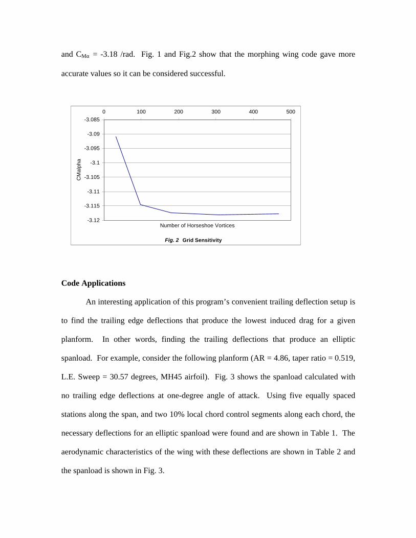
and CMα = -3.18 /rad. Fig. 1 and Fig.2 show that the morphing wing code gave more

accurate values so it can be considered successful.

Code Applications

An interesting application of this program’s convenient trailing deflection setup is

to find the trailing edge deflections that produce the lowest induced drag for a given

planform. In other words, finding the trailing deflections that produce an elliptic

spanload. For example, consider the following planform (AR = 4.86, taper ratio = 0.519,

L.E. Sweep = 30.57 degrees, MH45 airfoil). Fig. 3 shows the spanload calculated with

no trailing edge deflections at one-degree angle of attack. Using five equally spaced

stations along the span, and two 10% local chord control segments along each chord, the

necessary deflections for an elliptic spanload were found and are shown in Table 1. The

aerodynamic characteristics of the wing with these deflections are shown in Table 2 and

the spanload is shown in Fig. 3.

Fig. 2 Grid Sensitivity

-3.12

-3.115

-3.11

-3.105

-3.1

-3.095

-3.09

-3.0850 100 200 300 400 500

Number of Horseshoe Vortices

CM

alph

a

Table 1 y/(b/2) defl (degrees)

0.2 -0.38 0.4 -0.89 0.6 -1.12 0.8 -2

1 -4.59 Table 2 VLM Output In degrees and 1/degrees CL alpha 0.067 CL twist 0.183 Cm alpha -0.006 Cm twist -0.035 Cm zero-lift -0.017 AoA zero-lift -2.753 e 0.991

Fig. 3

0 0.1 0.2 0.3 0.4 0.5 0.6 0.7 0.8 0.9 10

0.5

1

1.5

Spa

nloa

d

Vortex Lattice Results, AR=4.86, TR=.519, L.E. Sweep=30.57 deg.

Deflected Elliptic Undeflected

0 0.1 0.2 0.3 0.4 0.5 0.6 0.7 0.8 0.9 10.5

1

1.5

Cl/C

L

0 0.1 0.2 0.3 0.4 0.5 0.6 0.7 0.8 0.9 10

2

4

6

deg

rees

y/(b/2)

Sample Input File for MorphVLM % Input m-file Used for the morphing wing ma=1; % For a morphing analysis enter 1; for a standard analysis enter 2. CL=0.29; % Desired lift coefficient b=5; %Span tr=.519; % Taper Ratio cr=1.3712; % Root Chord Lenght LE=30.57; %Leading edge sweep (degrees) xcg=0.9125; % xcg, CM is referenced to this point. n=7; % # of chordwise vortices m=14; % # of spanwise vortices nribs=6; % The number of spanwise ribs aa=2; % Enter the number of segments that make up the control surface sribs=[.25 .25 .25 .25 .25 .25;.15 .15 .15 .15 .15 .15]'; % Size of each control segment as a ratio of the local chord lenght, starting at the trailing edge. % sribs must be aa x 1 in size defl=[-3.1 -2.4 -1.623 -.82 -.52 -.3]'; rootdefl=-4; sroot=[.1;.1]; % size of the root deflection surface % defl must be nribs x 1 in size wostart=0.0; % The fraction of the half span at which the linear wash-out distribution begins. woang=4; % Wash-out angle of the wing-tip (degrees), assumes linear distribution startin at wostart. meancamber='-2.602*xc^6+8.926*xc^5-11.97*xc^4+8.0976*xc^3-3.0462*xc^2+0.591*xc'; % equation for the mean camber line of the airfoil used. slw=1 % slw == 1 for a straight line wrap, assumes theta_root=0. alphazlcorr=-3; % predicted difference between actual and calculated zero-lift angle.

Appendix 2. An Introduction to the Morphing Wing Vortex Lattice Program

(MorphVLM)

Program Purpose and Limitations

This MATLAB program MorphVLM was written for the purpose of quickly

analyzing the aerodynamic effects of varying the twist and trailing edge shape of a lifting

surface. The program uses a standard vortex lattice method with equally distributed

horseshoe vortices. It was designed with a flying wing in mind, so it currently analyzes

only a single lifting surface with no dihedral.

The main advantage of this program over other vlm codes known to the author is

the ease at which control deflections are modeled. This program handles control

deflections by having the user define a certain number of spanwise stations on the trailing

edge at which deflection angles are defined. There is then a linear distribution between

each defined point along the span. The way at which each airfoil is deformed to provide

the desired trailing deflections is determined by the number of chordwise segments and

their size relative to the local chord. The program automatically calculates the slope of

the mean camber line at the ¾ point of each horseshoe vortex.

Input

The input style found most convenient by the author consists of defining all of the

necessary input information in an m-file. This may be a somewhat nonstandard approach

to program input, but it’s quick, easy and effective. Also, once the program is ran for a

certain planform and the MATLAB command window is kept open, subsequent control

deflection and twist cases can be run quickly without recalculating the vortex layout.

This is why the program asks if the same planform is being repeated. The required input

information is as follows:

(MATLAB is case sensitive)

ma = enter 1 if control deflections and twist are to be analyzed; enter 2 to ignore control

deflections and twist.

AOA = This is the angle of attack in degrees that CL, CM and e are calculated for.

b = Wingspan

tr = Taper Ratio

cr = Root chord length

LE = Leading edge sweep (degrees)

xcg = Distance from the wing apex to the center of gravity, this is the reference location

for CM.

n = Number of chordwise horseshoe vortices.

m = Number of spanwise horseshoe vortices.

nribs = Number of equally spaced spanwise sections where control deflections are to be

specified.

aa = Number of chordwise sections that make up each control surface.

sribs = An [nribs x aa] matrix that specifies the size of each control section as a fraction

of the local chord. The first row of sribs specifies the most inboard rib, and the first

column specifies the trailing edge section.

defl = An [nribs x 1] matrix that specifies the deflection of the trailing edge of each of

the nribs, with the first entry specifying the most inboard section.

rootdefl = Specifies the deflection angle of the trailing edge of the root (this is not

considered in defl because the wing root is not considered a rib.

sroot = An [aa x 1] matrix that specifies the size of the root control surface.

wostart = The spanwise location where the twist begins as a fraction of the half-span.

wo = Twist angle with positive being wash-out (degrees).

slw = Enter 1 for a straight-line wrap distribution.

meancamber = Equation for the mean camber line of the desired airfoil, xc should be

used as the x-variable.

alphazlcorr = Predicted difference between the actual and calculated zero-lift angle of

attack (deg), a value of -3 is recommended.

Running the Program

Save all of the files for the program in the same directory. Then type in the name

of the input file. Last, type in the MorphVLM and the program should run. The program

will ask if you want to do a complete calculation. This is done because if the same

planform with different deflections are run, the entire program does not have to be over

and over. Always enter 2 if it is the first run of the program.

Output

A listing of various aerodynamic characteristics is displayed each time the

program is run. But, there are many more that are not listed after each run. The

following are the names used to call up the program’s calculated aerodynamic

characteristics.

CL= Lift coefficient at the defined angle of attack.

CM = Pitching moment at the defined angle of attack.

CLalpha = Lift coefficient per-degree alpha.

CMalpha = Pitching moment coefficient per-degree alpha (referenced to the C.G, the

mean geometric chord is used to non-dimensionalize the moment coefficients.).

CLtwist = Lift coefficient due to camber, wing twist, and control deflections.

CMtwist = Pitching moment coefficient due to camber, wing twist, and control.

CMzl = Zero-lift pitching moment coefficient.

alpha_zero_lift = Zero-lift angle of attack (degrees).

hac = The location of the aerodynamic center on the mean aerodynamic chord.

ycp = The y-location of the center of pressure as a fraction of the span.

cwcirc = [m x 1] vector containing the total spanload.

tcwcirc = [m x 1] vector containing the spanload due to twist and camber only.

pdcwcirc = [m x 1] vector containing the spanload due to angle of attack only

deltacp = [m x n] matrix containing the delta CP from each horseshoe vortex.

xmac = Distance from the wing apex to the leading edge of the mean aerodynamic chord.

cmac = Length of the mean aerodynamic chord.

xac = Distance from the wing apex to the aerodynamic center.

sweep_qc = sweep angle of the quarter chord (rad).

Clcorr = Distribution of local lift coefficients along the span corrected for a 2-D analysis

using the cosine squared rule.

CLtrim = Lift coefficient that the wing would trim at with the given deflections

alphatrim = Angle of attack that the wing would trim at with the given deflections (deg).

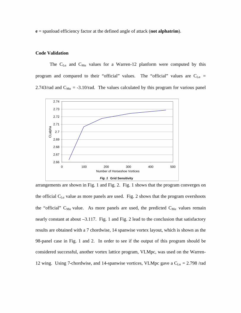
e = spanload efficiency factor at the defined angle of attack (not alphatrim).

Code Validation

The CLα and CMα values for a Warren-12 planform were computed by this

program and compared to their “official” values. The “official” values are CLα =

2.743/rad and CMα = -3.10/rad. The values calculated by this program for various panel

arrangements are shown in Fig. 1 and Fig. 2. Fig. 1 shows that the program converges on

the official CLα value as more panels are used. Fig. 2 shows that the program overshoots

the “official” CMα value. As more panels are used, the predicted CMα values remain

nearly constant at about –3.117. Fig. 1 and Fig. 2 lead to the conclusion that satisfactory

results are obtained with a 7 chordwise, 14 spanwise vortex layout, which is shown as the

98-panel case in Fig. 1 and 2. In order to see if the output of this program should be

considered successful, another vortex lattice program, VLMpc, was used on the Warren-

12 wing. Using 7-chordwise, and 14-spanwise vortices, VLMpc gave a CLα = 2.798 /rad

Fig. 1 Grid Sensitivity

2.66

2.67

2.68

2.69

2.7

2.71

2.72

2.73

2.74

0 100 200 300 400 500Number of Horseshoe Vortices

CLa

lpha

and CMα = -3.18 /rad. Fig. 1 and Fig.2 show that the morphing wing code gave more

accurate values so it can be considered successful.

Code Applications

An interesting application of this program’s convenient trailing deflection setup is

to find the trailing edge deflections that produce the lowest induced drag for a given

planform. In other words, finding the trailing deflections that produce an elliptic

spanload. For example, consider the following planform (AR = 4.86, taper ratio = 0.519,

L.E. Sweep = 30.57 degrees, MH45 airfoil). Fig. 3 shows the spanload calculated with

no trailing edge deflections at one-degree angle of attack. Using five equally spaced

stations along the span, and two 10% local chord control segments along each chord, the

necessary deflections for an elliptic spanload were found and are shown in Table 1. The

aerodynamic characteristics of the wing with these deflections are shown in Table 2 and

the spanload is shown in Fig. 3.

Fig. 2 Grid Sensitivity

-3.12

-3.115

-3.11

-3.105

-3.1

-3.095

-3.09

-3.0850 100 200 300 400 500

Number of Horseshoe Vortices

CM

alph

a

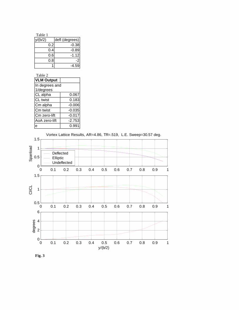
Table 1 y/(b/2) defl (degrees)

0.2 -0.38 0.4 -0.89 0.6 -1.12 0.8 -2

1 -4.59 Table 2 VLM Output In degrees and 1/degrees CL alpha 0.067 CL twist 0.183 Cm alpha -0.006 Cm twist -0.035 Cm zero-lift -0.017 AoA zero-lift -2.753 e 0.991

Fig. 3

0 0.1 0.2 0.3 0.4 0.5 0.6 0.7 0.8 0.9 10

0.5

1

1.5

Spa

nloa

d

Vortex Lattice Results, AR=4.86, TR=.519, L.E. Sweep=30.57 deg.

Deflected Elliptic Undeflected

0 0.1 0.2 0.3 0.4 0.5 0.6 0.7 0.8 0.9 10.5

1

1.5

Cl/C

L

0 0.1 0.2 0.3 0.4 0.5 0.6 0.7 0.8 0.9 10

2

4

6

deg

rees

y/(b/2)

Sample Input File for MorphVLM % Input m-file Used for the morphing wing ma=1; % For a morphing analysis enter 1; for a standard analysis enter 2. CL=0.29; % Desired lift coefficient b=5; %Span tr=.519; % Taper Ratio cr=1.3712; % Root Chord Lenght LE=30.57; %Leading edge sweep (degrees) xcg=0.9125; % xcg, CM is referenced to this point. n=7; % # of chordwise vortices m=14; % # of spanwise vortices nribs=6; % The number of spanwise ribs aa=2; % Enter the number of segments that make up the control surface sribs=[.25 .25 .25 .25 .25 .25;.15 .15 .15 .15 .15 .15]'; % Size of each control segment as a ratio of the local chord lenght, starting at the trailing edge. % sribs must be aa x 1 in size defl=[-3.1 -2.4 -1.623 -.82 -.52 -.3]'; rootdefl=-4; sroot=[.1;.1]; % size of the root deflection surface % defl must be nribs x 1 in size wostart=0.0; % The fraction of the half span at which the linear wash-out distribution begins. woang=4; % Wash-out angle of the wing-tip (degrees), assumes linear distribution startin at wostart. meancamber='-2.602*xc^6+8.926*xc^5-11.97*xc^4+8.0976*xc^3-3.0462*xc^2+0.591*xc'; % equation for the mean camber line of the airfoil used. slw=1 % slw == 1 for a straight line wrap, assumes theta_root=0. alphazlcorr=-3; % predicted difference between actual and calculated zero-lift angle.

Appendix 3. Construction Documentation for the PZT Model § Cut out wings from blue insulation foam using hot wire

– Created templates for both upper and lower surfaces which would guide the hot wire

– Sand down templates until nice and smooth, any ridges would cause the hot wire to jump causing imperfections

– Attach templates to foam and set weights on top of foam to hold it in one place as the wire cuts through

– Set bow on cutting plane line and attach weights to bow – As current is applied to the wire it will begin to cut through the foam and

the weight will pull it through – Repeat for other surface

§ Sand wings down for a smooth finish § Cut at quarter chord and PZT mounting point to separate trailing edge apart from

leading edge § Building the Wing Box, Cover leading edge in fiberglass

– Sand the two foam wing halves – Weigh the two wing halves, 4.75 oz – Cut each wing half at the ¼ chord line – Cut each wing half at the PZT mounting line – Bond the two halves of the wing section between the ¼ chord line and the

PZT mounting line – Pre-cut two pieces of fiberglass cloth that will fit onto the foam at the ¼

chord line – Epoxy the fiberglass so that it is flush with the surface of the foam – Weigh entire foam wing structure with complete fiberglass spar, 6.45 oz – Pre-cut two pieces of fiberglass that will envelope the entire foam wing

structure – Epoxy first wrap of fiberglass onto the foam wing structure, allow one day

for it to dry – Lightly sand off any imperfections that came up while drying – Weigh wing box structure with one ply of fiberglass, 15.25 oz – Use epoxy filler compound to fill in any large dips or grooves on first ply

of fiberglass, allow one day for it to dry – Epoxy second wrap of fiberglass onto the wing box structure, allow

another day to dry – Once again sand off any imperfections that came up while drying – Weigh the wing box with two wraps of fiberglass, 21.95 oz – Apply light coat of epoxy filler to fill in any holes or grooves and leave a

smooth surface exposed to flow

§ Attach an aluminum bar/ foam box, which have been covered in fiberglass, to the center section of the plane which will be the mounting platform for controls, and will distribute the load from the wind tunnel mounting bracket.

§ Cowling Creation – Create mold from cardboard and a Styrofoam nose – Cover in plastic wrap – Lay Fiberglass over mold – Separate Cowling from mold – Attach Velcro patches to the plane along with the fuselage for mounting

which allows easy accessibility to the controls § Mount PZTs to wings

– Eight PZT’s will be used total with four on each half span – Drill counter-sunk mounting holes into an L-shaped piece of plastic. – Attach PZT’s onto plastic-L with screws and nuts. – Secure electrical leads onto PZT’s – File down slots on trailing edge at angles at which the PZT’s will fit into

in order to maintain the proper shape of the airfoil. – Attach PZT’s to trailing edge using two faced tape.

§ Apply skin to cover section between leading and trailing edge § Final touch ups, 42.35 oz.

Template Construction

Setting up the hot wire and attaching templates

Using the hot wire to cut out the wing box

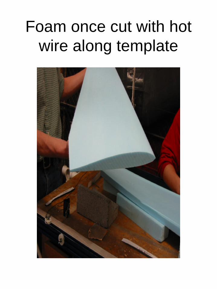
Foam once cut with hot wire along template

Cutting the wings at quarter chord and the PZT

mounting point

Finished wing sections once cut out from hot wire

Leading edge before and after fiberglass process

Mounting of the PZTs

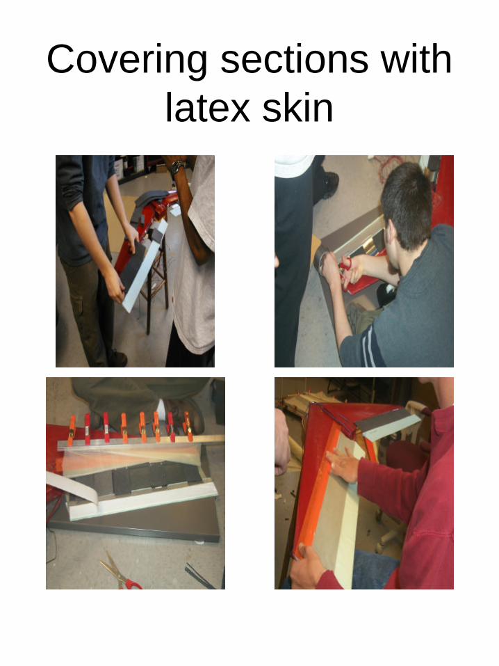
Covering sections with latex skin

The finished product