Embed Size (px)
Citation preview
SAP COMMUNITY NETWORK SDN - sdn.sap.com | BPX - bpx.sap.com | BOC - boc.sap.com | UAC - uac.sap.com
© 2011 SAP AG 1
SAP Business Objects – More
Reporting against OLAP data from
Microsoft Analysis Services and
Oracle Hyperion Essbase
Applies to:
SAP BusinessObjects XI 4.0 Feature Support Package 4, the information design tool, Web Intelligence, Microsoft Analysis Services 2008 and Oracle Hyperion Essbase 11. For more information, visit the Business Objects homepage.
Summary
This paper continues a series of articles covering common reporting scenarios on OLAP cubes. The series started with the articles Profiling and Bucketing OLAP members and Reporting against OLAP data. The present article develops additional reporting use cases: DSO financial ratio, multi-source document, trend analysis and current user filter. You can find the examples presented here.
Author: Marc Daniau
Company: SAP
Created on: 26 October 2012
Author Bio
Marc Daniau joined Business Objects in 1992 as project consultant in France. He moved to the product group in San Jose in 1998 to work on EPM products. He moved back to Paris in 2003 to work within the semantic layer team.
SAP Business Objects – More Reporting against OLAP data from Microsoft Analysis Services and Oracle Hyperion Essbase
SAP COMMUNITY NETWORK SDN - sdn.sap.com | BPX - bpx.sap.com | BOC - boc.sap.com | UAC - uac.sap.com
© 2012 SAP AG 2
Table of Contents
Number of days in period .................................................................................................................................... 3
Adjusted Value ................................................................................................................................................ 3
Days Sales Outstanding.................................................................................................................................. 6
Multi-source document ....................................................................................................................................... 8
Merging data from two cubes .......................................................................................................................... 8
Combining OLAP data with relational data ................................................................................................... 13
Trend analysis .................................................................................................................................................. 19
Smoothing ..................................................................................................................................................... 19
Curve fitting ................................................................................................................................................... 22
Current User Filter ............................................................................................................................................ 26
User stored as an attribute ............................................................................................................................ 26
User as a member of a parent-child hierarchy .............................................................................................. 28
Enforced filter ................................................................................................................................................ 30
Related Content ................................................................................................................................................ 33
Copyright........................................................................................................................................................... 34
SAP Business Objects – More Reporting against OLAP data from Microsoft Analysis Services and Oracle Hyperion Essbase
SAP COMMUNITY NETWORK SDN - sdn.sap.com | BPX - bpx.sap.com | BOC - boc.sap.com | UAC - uac.sap.com
© 2012 SAP AG 3
Number of days in period
Among the indicators involving in their formula the number of days in the period that is being analyzed, we find the financial ratio Days Sales Outstanding (DSO) that many companies use. The number of days can serve in other situations where the business user must normalize the data in order to fairly compare periods of unequal lengths for instance.
Adjusted Value
How can we obtain the number of days for each month or each quarter? The answer to that question depends on the structure of the OLAP cube. If the cube includes a time hierarchy like Year>Quarter>Month>Day we can simply count the day members for the current time period. We will cover that case in our next section. However if the time hierarchy stops at the month level, we must adopt a different approach. In that case, we can leverage the date functions provided by the MDX engine as illustrated in the coming example.
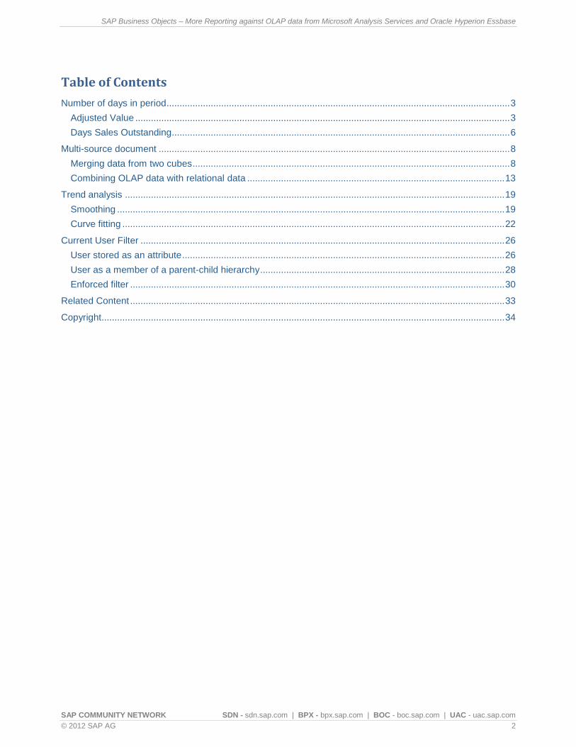
The Essbase cube „ASOsamp.Sample‟ has the following structure with respect to the time dimension.
With a universe against that cube, we are able to compute the number of days by months for the current year as well as the previous year.

SAP Business Objects – More Reporting against OLAP data from Microsoft Analysis Services and Oracle Hyperion Essbase
SAP COMMUNITY NETWORK SDN - sdn.sap.com | BPX - bpx.sap.com | BOC - boc.sap.com | UAC - uac.sap.com
© 2012 SAP AG 4
Here is the underlying query.
We added four calculated measures to the business layer to make the query possible.
We took advantage of the time functions provided by Essbase 11 to build those measures.
Name Expression of the calculated measure
Today's Year
DatePart(Today(),DP_YEAR)
Year Number
IIF( IS([Years].CurrentMember, [Current Year]), @Select(Years\Today's Year), IIF( IS([Years].CurrentMember, [Previous Year]), @Select(Years\Today's Year) -1 , MISSING))
1st day of month
TodateEx( "mon dd yyyy" , concat([Time].CurrentMember.MEMBER_NAME , " 01 " , Left(NumToStr(@Select(Years\Year Number)),1) , Substring(NumToStr(@Select(Years\Year Number)),3,5)) )
Days in Month
DatePart(GetLastDay(@Select(Time\1st day of month), DP_MONTH), DP_DAY )
With the same approach we can obtain the number of days by quarters.
Name Expression of the calculated measure
1st day of quarter
TodateEx( "mon dd yyyy" , concat(Head(Descendants([Time].CurrentMember, [Months])).Item(0).Item(0).MEMBER_NAME , " 01 " , Left(NumToStr(@Select(Years\Year Number)),1) , Substring(NumToStr(@Select(Years\Year Number)),3,5)) )
Last day in quarter
GetLastDay(TodateEx( "mon dd yyyy" , concat(Tail(Descendants([Time].CurrentMember, [Months])).Item(0).Item(0).MEMBER_NAME , " 01 " , Left(NumToStr(@Select(Years\Year Number)),1) , Substring(NumToStr(@Select(Years\Year Number)),3,5)) ), DP_MONTH)
Days in Quarter
DateDiff( @Select(Time\1st day of quarter), @Select(Time\Last day in quarter), DP_DAY ) +1
SAP Business Objects – More Reporting against OLAP data from Microsoft Analysis Services and Oracle Hyperion Essbase
SAP COMMUNITY NETWORK SDN - sdn.sap.com | BPX - bpx.sap.com | BOC - boc.sap.com | UAC - uac.sap.com
© 2012 SAP AG 5
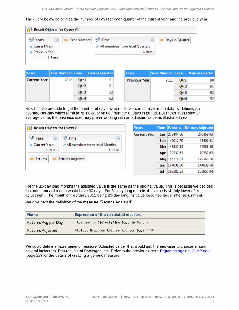
The query below calculates the number of days for each quarter of the current year and the previous year.
Now that we are able to get the number of days by periods, we can normalize the data by defining an average-per-day which formula is: indicator value / number of days in period. But rather than using an average value, the business user may prefer working with an adjusted value as illustrated next.
For the 30-day long months the adjusted value is the same as the original value. This is because we decided that our standard month would have 30 days. For 31-day long months the value is slightly lower after adjustment. The month of February 2012 being 29-day long, its value becomes larger after adjustment.
We give next the definition of the measure “Returns Adjusted”.
Name Expression of the calculated measure
Returns Avg per Day [Returns] / @Select(Time\Days in Month)
Returns Adjusted @Select(Measures\Returns Avg per Day) * 30
We could define a more generic measure “Adjusted value” that would ask the end-user to choose among several indicators: Returns, Nb of Packages, etc. Refer to the previous article Reporting against OLAP data (page 27) for the details of creating a generic measure.
SAP Business Objects – More Reporting against OLAP data from Microsoft Analysis Services and Oracle Hyperion Essbase
SAP COMMUNITY NETWORK SDN - sdn.sap.com | BPX - bpx.sap.com | BOC - boc.sap.com | UAC - uac.sap.com
© 2012 SAP AG 6
Days Sales Outstanding
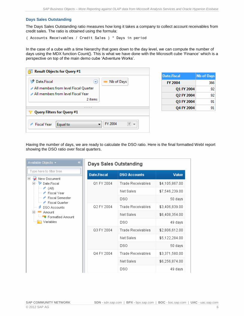
The Days Sales Outstanding ratio measures how long it takes a company to collect account receivables from credit sales. The ratio is obtained using the formula:
( Accounts Receivables / Credit Sales ) * Days in period
In the case of a cube with a time hierarchy that goes down to the day level, we can compute the number of days using the MDX function Count(). This is what we have done with the Microsoft cube „Finance‟ which is a perspective on top of the main demo cube „Adventure Works‟.
Having the number of days, we are ready to calculate the DSO ratio. Here is the final formatted WebI report showing the DSO ratio over fiscal quarters.
SAP Business Objects – More Reporting against OLAP data from Microsoft Analysis Services and Oracle Hyperion Essbase
SAP COMMUNITY NETWORK SDN - sdn.sap.com | BPX - bpx.sap.com | BOC - boc.sap.com | UAC - uac.sap.com
© 2012 SAP AG 7
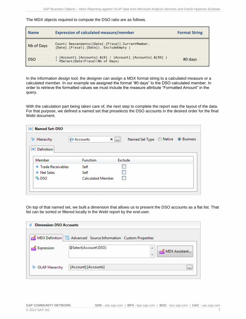
The MDX objects required to compute the DSO ratio are as follows.
Name Expression of calculated measure/member Format String
Nb of Days Count( Descendants([Date].[Fiscal].CurrentMember, [Date].[Fiscal].[Date]), ExcludeEmpty )
DSO ( [Account].[Accounts].&[6] / [Account].[Accounts].&[50] ) * @Select(Date\Fiscal\Nb of Days)
#0 days
In the information design tool, the designer can assign a MDX format string to a calculated measure or a calculated member. In our example we assigned the format “#0 days” to the DSO calculated member. In order to retrieve the formatted values we must include the measure attribute “Formatted Amount” in the query.
With the calculation part being taken care of, the next step to complete the report was the layout of the data. For that purpose, we defined a named set that preselects the DSO accounts in the desired order for the final WebI document.
On top of that named set, we built a dimension that allows us to present the DSO accounts as a flat list. That list can be sorted or filtered locally in the WebI report by the end-user.

SAP Business Objects – More Reporting against OLAP data from Microsoft Analysis Services and Oracle Hyperion Essbase
SAP COMMUNITY NETWORK SDN - sdn.sap.com | BPX - bpx.sap.com | BOC - boc.sap.com | UAC - uac.sap.com
© 2012 SAP AG 8
Multi-source document
In this chapter, we will see how to bring data from multiple sources into a single WebI document.
Merging data from two cubes
Some companies organize their data in such a way that the actual numbers are stored in one cube whereas the forecast or budget numbers are stored in another cube. And of course the business users need to view the data from both cubes into a single line chart. Those two cubes are likely to have different levels of granularity, actuals being stored at a finer grain than forecasts or budgets. Provided they share common dimensions like time and product, we can combine the actual and forecast data using the merge feature provided by Web Intelligence.
The business user requests to be able to choose the point in time when the actual line must stop. Passed that point, we must display the forecast/budget values. The forecast or budget having different versions or types, we must let the user choose the appropriate version or type when running the query.
With the above requirements in mind, let us build a line chart with actual and forecast data combined. For the sake of the exercise we will use the Essbase demo cube „Sample.Basic„ for the actual data and the Essbase demo cube „Samppart.Company‟ for the budget data.
To begin with, we generate from the information design tool, two business layers against those cubes. In order to allow the user to choose the month when the actual line should stop, we must define a prompt. A named set and a dimension are added to the business layer HYP_ACTUAL so that we can retrieve the list of months.
Their expressions are given below.
Name Expression of the named set or the dimension
Month {[Year].[Months].Members}
Months @Select(Year\Month)
We then define a list of values “List of Months” based upon the dimension Months.

SAP Business Objects – More Reporting against OLAP data from Microsoft Analysis Services and Oracle Hyperion Essbase
SAP COMMUNITY NETWORK SDN - sdn.sap.com | BPX - bpx.sap.com | BOC - boc.sap.com | UAC - uac.sap.com
© 2012 SAP AG 9
The prompt “As Of Month” is created that refers to the list of values we have just defined. We assign May as the default value.
When the prompt has been defined and tested within the business layer HYP_ACTUAL, we can copy it with its related objects to the second business layer HYP_BUDGET.
The next step consists of preparing the calculated measures required to produce our report on two separate cubes. After completion, the two business layers look like this.
The measures “Month Number” and “As Of Month Number” are identical in both business layers. One can copy those measures from one business layer to the other.
As for the measures “Actual aom” and “Budget aom” they adjust themselves according to the month period selected by the end-user. They behave in a synchronized manner thanks to the identical prompt “As Of Month”. Their definitions are given in the following table.
SAP Business Objects – More Reporting against OLAP data from Microsoft Analysis Services and Oracle Hyperion Essbase
SAP COMMUNITY NETWORK SDN - sdn.sap.com | BPX - bpx.sap.com | BOC - boc.sap.com | UAC - uac.sap.com
© 2012 SAP AG 10
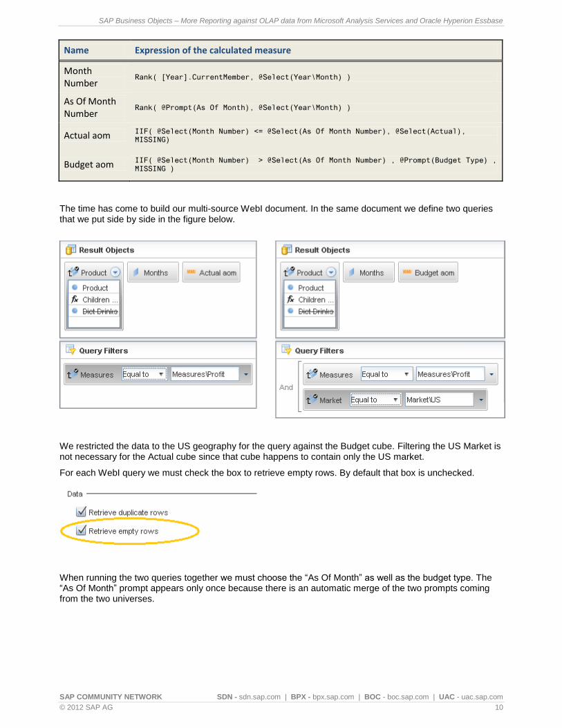
Name Expression of the calculated measure
Month Number
Rank( [Year].CurrentMember, @Select(Year\Month) )
As Of Month Number
Rank( @Prompt(As Of Month), @Select(Year\Month) )
Actual aom IIF( @Select(Month Number) <= @Select(As Of Month Number), @Select(Actual), MISSING)
Budget aom IIF( @Select(Month Number) > @Select(As Of Month Number) , @Prompt(Budget Type) , MISSING )
The time has come to build our multi-source WebI document. In the same document we define two queries that we put side by side in the figure below.
We restricted the data to the US geography for the query against the Budget cube. Filtering the US Market is not necessary for the Actual cube since that cube happens to contain only the US market.
For each WebI query we must check the box to retrieve empty rows. By default that box is unchecked.
When running the two queries together we must choose the “As Of Month” as well as the budget type. The “As Of Month” prompt appears only once because there is an automatic merge of the two prompts coming from the two universes.

SAP Business Objects – More Reporting against OLAP data from Microsoft Analysis Services and Oracle Hyperion Essbase
SAP COMMUNITY NETWORK SDN - sdn.sap.com | BPX - bpx.sap.com | BOC - boc.sap.com | UAC - uac.sap.com
© 2012 SAP AG 11
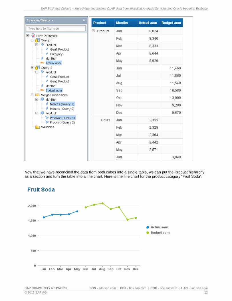
The WebI default report presents one table per query.
After merging the two queries on product and on month using the merge functionality of Web Intelligence, we get rid of the two default tables and display the data within a single table as follows.
SAP Business Objects – More Reporting against OLAP data from Microsoft Analysis Services and Oracle Hyperion Essbase
SAP COMMUNITY NETWORK SDN - sdn.sap.com | BPX - bpx.sap.com | BOC - boc.sap.com | UAC - uac.sap.com
© 2012 SAP AG 12
Now that we have reconciled the data from both cubes into a single table, we can put the Product hierarchy as a section and turn the table into a line chart. Here is the line chart for the product category “Fruit Soda”.
SAP Business Objects – More Reporting against OLAP data from Microsoft Analysis Services and Oracle Hyperion Essbase
SAP COMMUNITY NETWORK SDN - sdn.sap.com | BPX - bpx.sap.com | BOC - boc.sap.com | UAC - uac.sap.com
© 2012 SAP AG 13
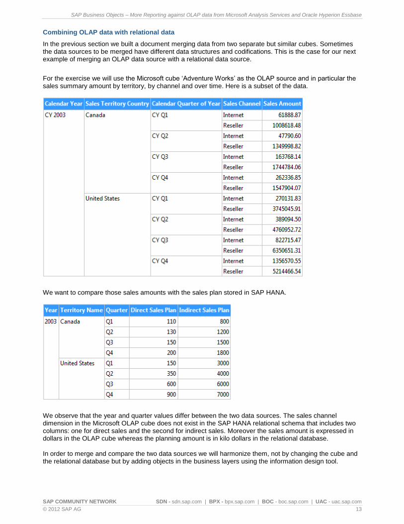
Combining OLAP data with relational data
In the previous section we built a document merging data from two separate but similar cubes. Sometimes the data sources to be merged have different data structures and codifications. This is the case for our next example of merging an OLAP data source with a relational data source.
For the exercise we will use the Microsoft cube „Adventure Works‟ as the OLAP source and in particular the sales summary amount by territory, by channel and over time. Here is a subset of the data.
We want to compare those sales amounts with the sales plan stored in SAP HANA.
We observe that the year and quarter values differ between the two data sources. The sales channel dimension in the Microsoft OLAP cube does not exist in the SAP HANA relational schema that includes two columns: one for direct sales and the second for indirect sales. Moreover the sales amount is expressed in dollars in the OLAP cube whereas the planning amount is in kilo dollars in the relational database. In order to merge and compare the two data sources we will harmonize them, not by changing the cube and the relational database but by adding objects in the business layers using the information design tool.
SAP Business Objects – More Reporting against OLAP data from Microsoft Analysis Services and Oracle Hyperion Essbase
SAP COMMUNITY NETWORK SDN - sdn.sap.com | BPX - bpx.sap.com | BOC - boc.sap.com | UAC - uac.sap.com
© 2012 SAP AG 14
Let us start with the time members in SAP HANA. We add two objects in the relational business layer so that year and quarter are prefixed with „CY‟ and therefore match the year and quarter values in the Microsoft OLAP cube.
Name SQL Select Expression of the dimension
Calendar Year 'CY ' || MDS.PERIOD.THE_YEAR
Calendar Quarter 'CY ' || MDS.PERIOD.THE_QUARTER
To make the actual sales comparable with the sales plan we define, in the OLAP business layer, two calculated measures listed in the table below.
Name MDX Expression of the calculated measure
Internet Sales
( [Measures].[Sales Amount] , [Sales Channel].[Sales Channel].&[Internet] ) / 1000
Reseller Sales
( [Measures].[Sales Amount] , [Sales Channel].[Sales Channel].&[Reseller] ) / 1000
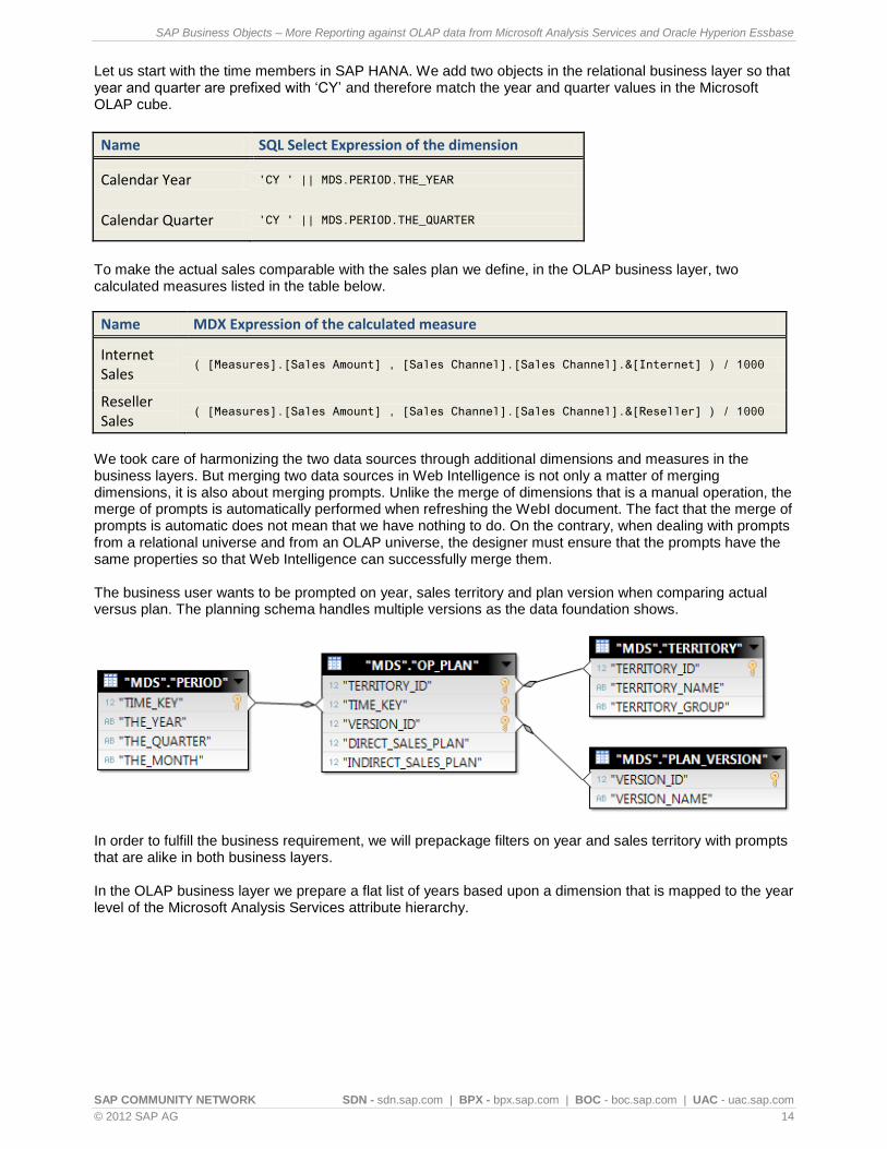
We took care of harmonizing the two data sources through additional dimensions and measures in the business layers. But merging two data sources in Web Intelligence is not only a matter of merging dimensions, it is also about merging prompts. Unlike the merge of dimensions that is a manual operation, the merge of prompts is automatically performed when refreshing the WebI document. The fact that the merge of prompts is automatic does not mean that we have nothing to do. On the contrary, when dealing with prompts from a relational universe and from an OLAP universe, the designer must ensure that the prompts have the same properties so that Web Intelligence can successfully merge them. The business user wants to be prompted on year, sales territory and plan version when comparing actual versus plan. The planning schema handles multiple versions as the data foundation shows.
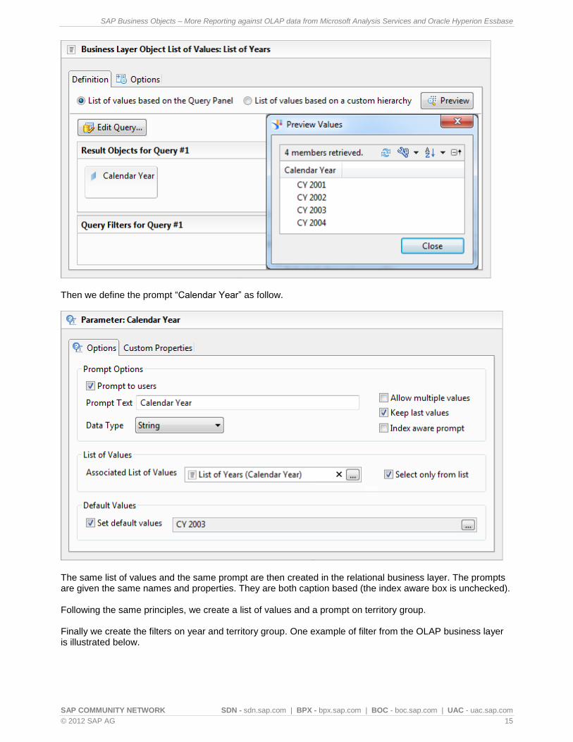
In order to fulfill the business requirement, we will prepackage filters on year and sales territory with prompts that are alike in both business layers. In the OLAP business layer we prepare a flat list of years based upon a dimension that is mapped to the year level of the Microsoft Analysis Services attribute hierarchy.
SAP Business Objects – More Reporting against OLAP data from Microsoft Analysis Services and Oracle Hyperion Essbase
SAP COMMUNITY NETWORK SDN - sdn.sap.com | BPX - bpx.sap.com | BOC - boc.sap.com | UAC - uac.sap.com
© 2012 SAP AG 15
Then we define the prompt “Calendar Year” as follow.
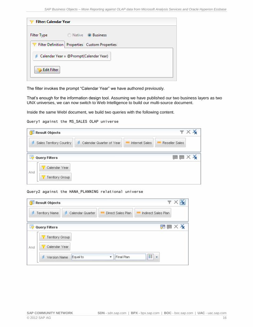
The same list of values and the same prompt are then created in the relational business layer. The prompts are given the same names and properties. They are both caption based (the index aware box is unchecked). Following the same principles, we create a list of values and a prompt on territory group. Finally we create the filters on year and territory group. One example of filter from the OLAP business layer is illustrated below.
SAP Business Objects – More Reporting against OLAP data from Microsoft Analysis Services and Oracle Hyperion Essbase
SAP COMMUNITY NETWORK SDN - sdn.sap.com | BPX - bpx.sap.com | BOC - boc.sap.com | UAC - uac.sap.com
© 2012 SAP AG 16
The filter invokes the prompt “Calendar Year” we have authored previously. That‟s enough for the information design tool. Assuming we have published our two business layers as two UNX universes, we can now switch to Web Intelligence to build our multi-source document. Inside the same WebI document, we build two queries with the following content. Query1 against the MS_SALES OLAP universe
Query2 against the HANA_PLANNING relational universe

SAP Business Objects – More Reporting against OLAP data from Microsoft Analysis Services and Oracle Hyperion Essbase
SAP COMMUNITY NETWORK SDN - sdn.sap.com | BPX - bpx.sap.com | BOC - boc.sap.com | UAC - uac.sap.com
© 2012 SAP AG 17
When hitting refresh the prompts box displays the two prompts „Calendar Year‟ and „Territory Group‟ common to both universes as well as the prompt „Plan Version‟ that is specific to the relational universe.
After running the two queries, we manually merge the two resulting data sets first on territory and then on quarter, thus obtaining two merged dimensions. Then we pick the objects highlighted in the figure below, and put them into a single table in the report.

SAP Business Objects – More Reporting against OLAP data from Microsoft Analysis Services and Oracle Hyperion Essbase
SAP COMMUNITY NETWORK SDN - sdn.sap.com | BPX - bpx.sap.com | BOC - boc.sap.com | UAC - uac.sap.com
© 2012 SAP AG 18
We format the report with two column charts side by side for each sales territory. One can compare over time the actuals in blue versus the plan in green. The direct sales are represented in the left graph while the indirect sales are represented in the right graph. The user responses to the prompts are displayed on the report header.
SAP Business Objects – More Reporting against OLAP data from Microsoft Analysis Services and Oracle Hyperion Essbase
SAP COMMUNITY NETWORK SDN - sdn.sap.com | BPX - bpx.sap.com | BOC - boc.sap.com | UAC - uac.sap.com
© 2012 SAP AG 19
Trend analysis
One essential dimension of OLAP cubes is the Time dimension. We have seen already in the article Reporting against OLAP data how to perform time comparisons and time rollups. Here we will focus on trend analysis techniques like smoothing and curve fitting. Those techniques may seem more geared towards interactive analysis and not so much towards reporting. However we have seen companies including in their reports moving averages on raw data that is too jagged. To report a trend indicator, some companies, instead of using the actual change between the current period and the previous period, are using the change estimate given by the trend slope over the last n periods.
The few examples that we will develop next to introduce moving-average and linear regression with MDX are taken from interactive workflows so that we can better visualize how smoothing and curve fitting work. As we just explained, those techniques can also be employed for reporting purposes. In the last exercise of this chapter, we will demonstrate the usage of linear regression to compute a trend indicator.
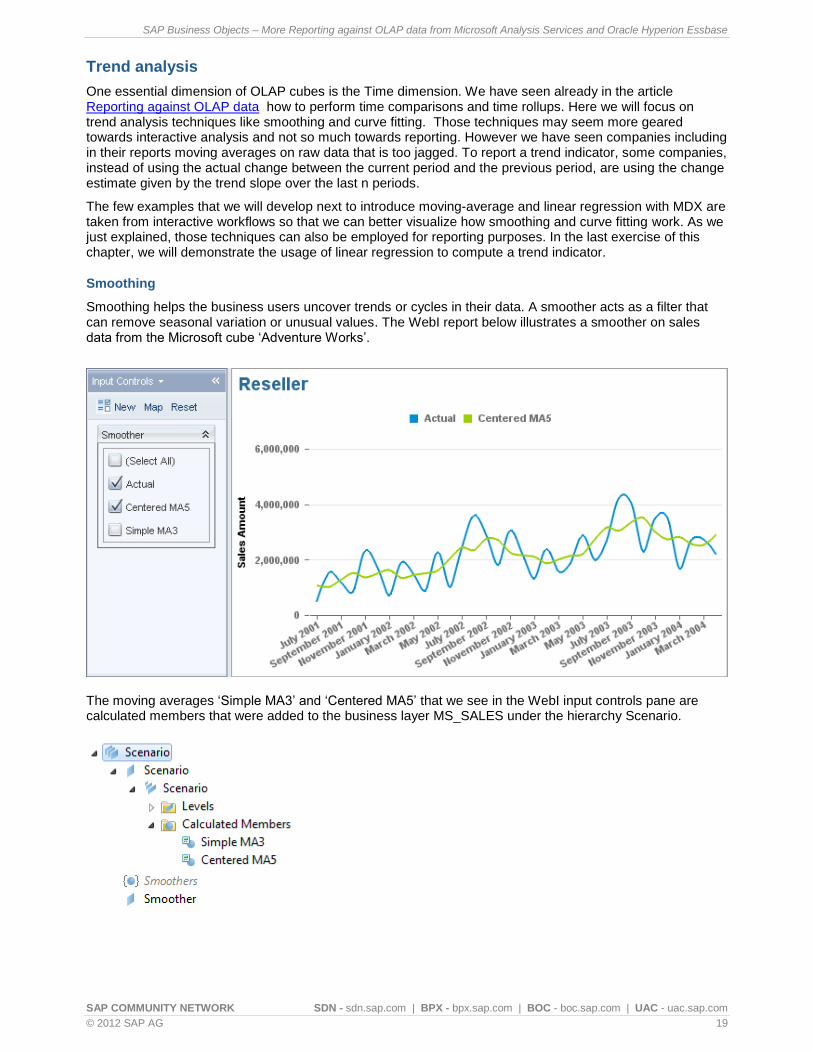
Smoothing
Smoothing helps the business users uncover trends or cycles in their data. A smoother acts as a filter that can remove seasonal variation or unusual values. The WebI report below illustrates a smoother on sales data from the Microsoft cube „Adventure Works‟.
The moving averages „Simple MA3‟ and „Centered MA5‟ that we see in the WebI input controls pane are calculated members that were added to the business layer MS_SALES under the hierarchy Scenario.
SAP Business Objects – More Reporting against OLAP data from Microsoft Analysis Services and Oracle Hyperion Essbase
SAP COMMUNITY NETWORK SDN - sdn.sap.com | BPX - bpx.sap.com | BOC - boc.sap.com | UAC - uac.sap.com
© 2012 SAP AG 20
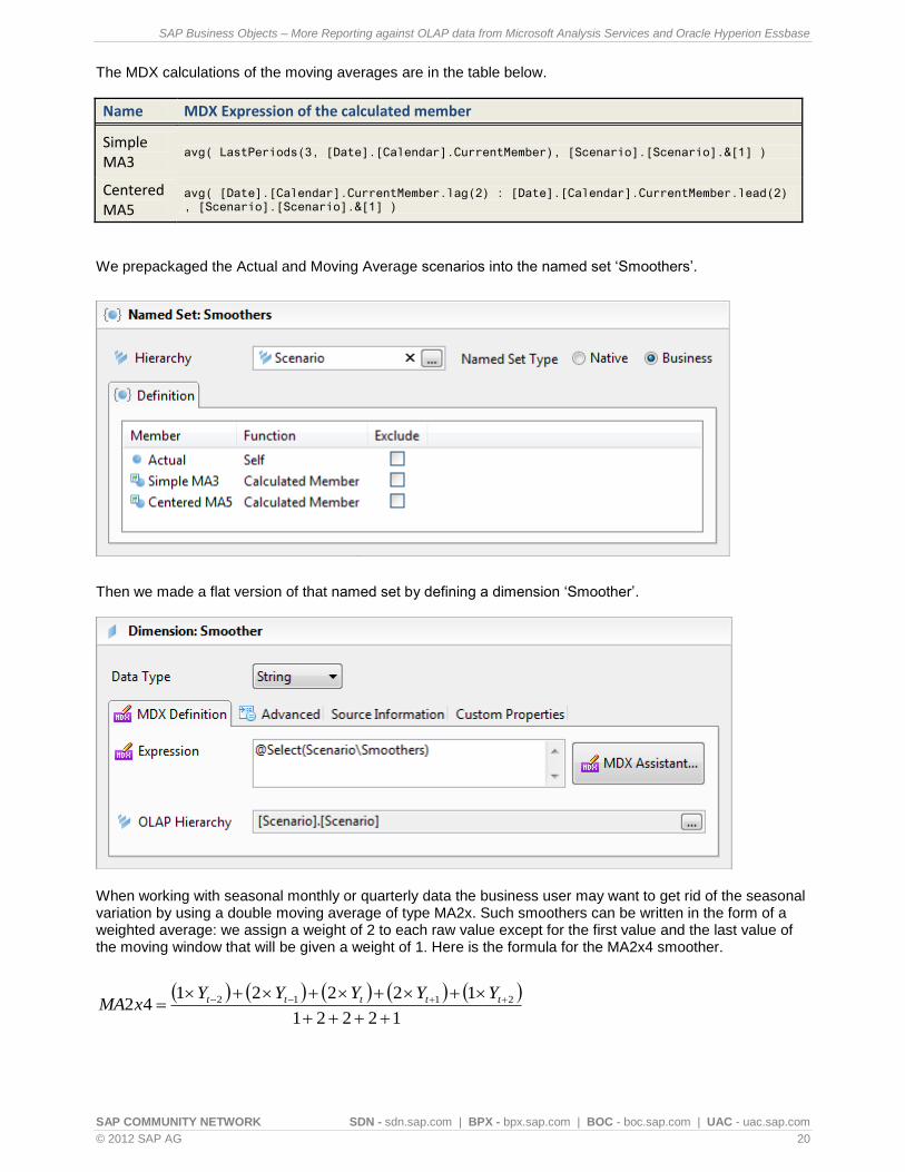
The MDX calculations of the moving averages are in the table below.
Name MDX Expression of the calculated member
Simple MA3
avg( LastPeriods(3, [Date].[Calendar].CurrentMember), [Scenario].[Scenario].&[1] )
Centered MA5
avg( [Date].[Calendar].CurrentMember.lag(2) : [Date].[Calendar].CurrentMember.lead(2) , [Scenario].[Scenario].&[1] )
We prepackaged the Actual and Moving Average scenarios into the named set „Smoothers‟.
Then we made a flat version of that named set by defining a dimension „Smoother‟.
When working with seasonal monthly or quarterly data the business user may want to get rid of the seasonal variation by using a double moving average of type MA2x. Such smoothers can be written in the form of a weighted average: we assign a weight of 2 to each raw value except for the first value and the last value of the moving window that will be given a weight of 1. Here is the formula for the MA2x4 smoother.
12221
1222142 2112
ttttt YYYYY
xMA

SAP Business Objects – More Reporting against OLAP data from Microsoft Analysis Services and Oracle Hyperion Essbase
SAP COMMUNITY NETWORK SDN - sdn.sap.com | BPX - bpx.sap.com | BOC - boc.sap.com | UAC - uac.sap.com
© 2012 SAP AG 21
We decided to trim the smoothed line when there are not enough data points to fill the requested span for calculating the double moving average as it occurs near the edges of the cube.
Name MDX Expression of the calculated member
MA2x4
IIF( count( Filter( {[Date].[Calendar].CurrentMember.lag(2) : [Date].[Calendar].CurrentMember.lead(2)} , ([Scenario].[Scenario].&[1], [Measures].[Order Quantity]) > 0)) = 5, ( sum( { [Date].[Calendar].CurrentMember.lag(2) , [Date].[Calendar].CurrentMember.lead(2) } , [Scenario].[Scenario].&[1] ) + sum( [Date].[Calendar].CurrentMember.lag(1) : [Date].[Calendar].CurrentMember.lead(1) , ([Scenario].[Scenario].&[1] * 2) ) ) / 8 , NULL )
MA2x8
IIF( count( Filter( {[Date].[Calendar].CurrentMember.lag(4) : [Date].[Calendar].CurrentMember.lead(4)}, ([Scenario].[Scenario].&[1], [Measures].[Order Quantity]) > 0)) = 9, ( sum( { [Date].[Calendar].CurrentMember.lag(4) , [Date].[Calendar].CurrentMember.lead(4) } , [Scenario].[Scenario].&[1] ) + sum( [Date].[Calendar].CurrentMember.lag(3) : [Date].[Calendar].CurrentMember.lead(3) , ([Scenario].[Scenario].&[1] * 2) ) ) / 16 , NULL)
MA2x12
IIF( count( Filter( {[Date].[Calendar].CurrentMember.lag(6) : [Date].[Calendar].CurrentMember.lead(6)} , ([Scenario].[Scenario].&[1], [Measures].[Order Quantity]) > 0)) = 13, ( sum( { [Date].[Calendar].CurrentMember.lag(6) , [Date].[Calendar].CurrentMember.lead(6) } , [Scenario].[Scenario].&[1] ) + sum( [Date].[Calendar].CurrentMember.lag(5) : [Date].[Calendar].CurrentMember.lead(5) , ([Scenario].[Scenario].&[1] * 2) ) ) / 24 , NULL)
Let us see the MA2x12 smoother in action on the monthly order quantity series.
Other kinds of smoothers can be used like moving median that is preferred to moving average for removing outliers.
Name MDX Expression of the calculated member
Simple MM3 median( LastPeriods(3, [Date].[Calendar].CurrentMember), [Scenario].[Scenario].&[1] )

SAP Business Objects – More Reporting against OLAP data from Microsoft Analysis Services and Oracle Hyperion Essbase
SAP COMMUNITY NETWORK SDN - sdn.sap.com | BPX - bpx.sap.com | BOC - boc.sap.com | UAC - uac.sap.com
© 2012 SAP AG 22
Curve fitting
A second technique for trend analysis is to fit a regression line to the data. The Microsoft MDX engine provides the necessary functions to compute the regression lines of common models. An example of curve fitting is given in the WebI report below.
The MDX calculations involved are these.
Name MDX Expression of the calculated measure/member
Period ID CINT([Date].[Calendar].CurrentMember.Properties(''ID''))
Fit Linear LinRegPoint( @Select(Time\Calendar\Period ID), @Select(Time\Calendar\Window), [Scenario].[Scenario].&[1], @Select(Time\Calendar\Period ID) )
Fit Exponential VBA, @Select(Time\Calendar\Window), VBA, @Select(Time\Calendar\Period ID) ))
Fit Hyperbola LinRegPoint( 1 / @Select(Time\Calendar\Period ID), @Select(Time\Calendar\Window), [Scenario].[Scenario].&[1], 1 / @Select(Time\Calendar\Period ID) )
We could have computed a sequence with the MDX function Rank on time members. Instead we used the time member internal ID that constitutes a predefined sequence representing the X variable. As we can see in the exponential fit expression, one can invoke vba functions like exp() or log() from a MDX expression in order to perform mathematical transformations.

SAP Business Objects – More Reporting against OLAP data from Microsoft Analysis Services and Oracle Hyperion Essbase
SAP COMMUNITY NETWORK SDN - sdn.sap.com | BPX - bpx.sap.com | BOC - boc.sap.com | UAC - uac.sap.com
© 2012 SAP AG 23
We will close this chapter with an example of trend indicator based upon the regression slope. Often we see reports with a trend indicator based upon the period-to-period change that is simply calculated as the difference between two data points: the current period and the previous period. The sign of the change value is supposed to tell whether the trend is going up or down. There is another method to obtain a trend indicator though that consists of calculating the slope of the regression line for the last, let‟s say, 6 periods. Just as with the actual change value, the sign of the slope value indicates whether the trend direction is upward or downward. Prior to building a WebI report showing a trend indicator, we must define two calculated members. For that we will use the business layer MS_SALES.
Name MDX Expression of the calculated member
6-pt Slope LinRegSlope( LastPeriods(6, [Date].[Calendar].CurrentMember), [Scenario].[Scenario].&[1], @Select(Time\Calendar\Period ID) )
6-pt Slope Direction
CASE WHEN @Select(Scenario\Scenario\Scenario\6-pt Slope) > 0 THEN 1 WHEN @Select(Scenario\Scenario\Scenario\6-pt Slope) < 0 THEN -1 ELSE 0 END
From there we define, attached to the Scenario hierarchy, a named set “Slope Indicator” that preselects the members required for our trend indicator report.
On top of that name set, we create the dimension “Trend Indicator”.
We may choose to set the status of the named-set to Hidden in order to simplify the business layer view of the end-user.
SAP Business Objects – More Reporting against OLAP data from Microsoft Analysis Services and Oracle Hyperion Essbase
SAP COMMUNITY NETWORK SDN - sdn.sap.com | BPX - bpx.sap.com | BOC - boc.sap.com | UAC - uac.sap.com
© 2012 SAP AG 24
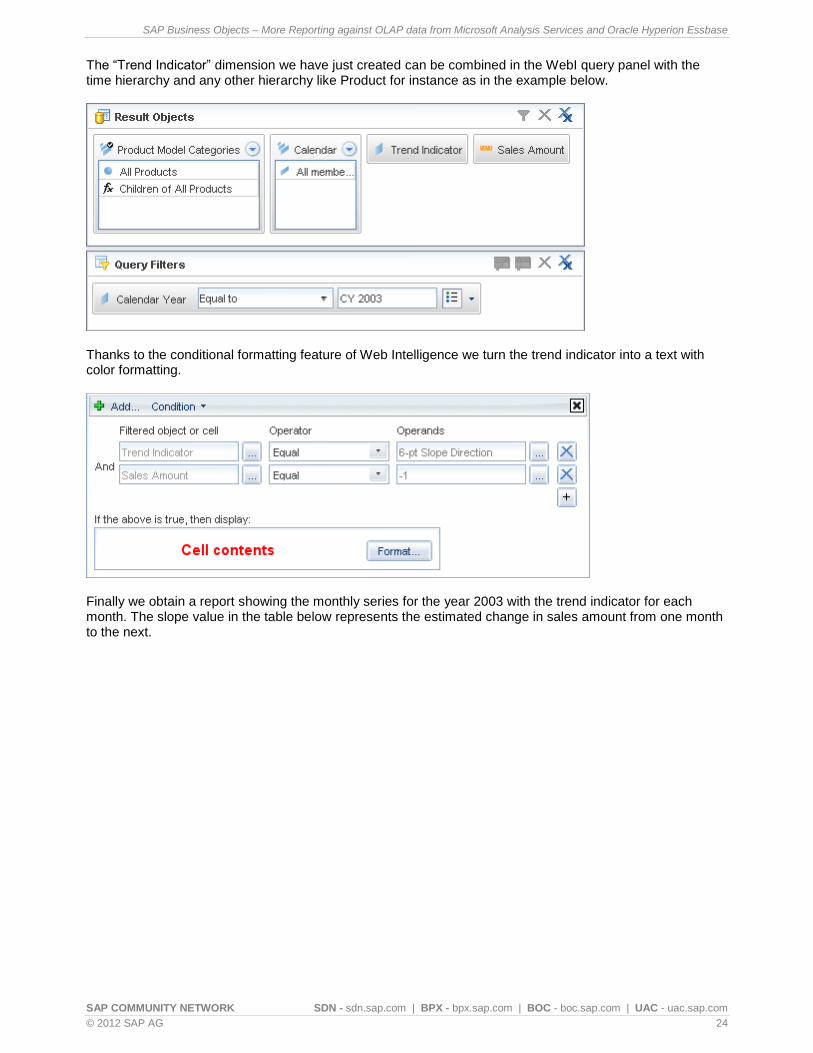
The “Trend Indicator” dimension we have just created can be combined in the WebI query panel with the time hierarchy and any other hierarchy like Product for instance as in the example below.
Thanks to the conditional formatting feature of Web Intelligence we turn the trend indicator into a text with color formatting.
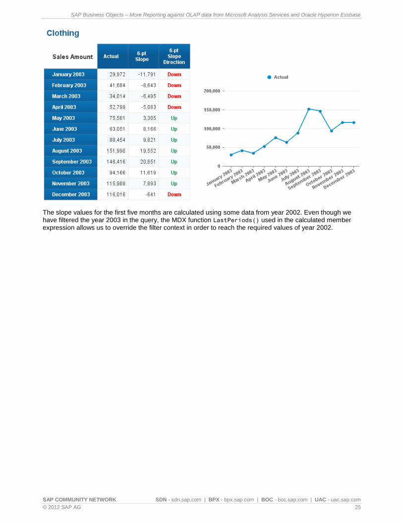
Finally we obtain a report showing the monthly series for the year 2003 with the trend indicator for each month. The slope value in the table below represents the estimated change in sales amount from one month to the next.
SAP Business Objects – More Reporting against OLAP data from Microsoft Analysis Services and Oracle Hyperion Essbase
SAP COMMUNITY NETWORK SDN - sdn.sap.com | BPX - bpx.sap.com | BOC - boc.sap.com | UAC - uac.sap.com
© 2012 SAP AG 25
The slope values for the first five months are calculated using some data from year 2002. Even though we have filtered the year 2003 in the query, the MDX function LastPeriods() used in the calculated member expression allows us to override the filter context in order to reach the required values of year 2002.

SAP Business Objects – More Reporting against OLAP data from Microsoft Analysis Services and Oracle Hyperion Essbase
SAP COMMUNITY NETWORK SDN - sdn.sap.com | BPX - bpx.sap.com | BOC - boc.sap.com | UAC - uac.sap.com
© 2012 SAP AG 26
Current User Filter
In our previous article we covered the requirement of filtering the data based upon the current date. For cubes that include individuals like store managers or sales representatives for instance, another requirement is to automatically filter based upon the current BusinessObjects user so that the BI user can focus on the data related to his own activity.
User stored as an attribute
The Essbase cube „ASOsamp.Sample‟ contains the store manager name as an attribute of the store dimension. A manager can be in charge of one brick & mortar store or/and one online store. Actually there is one exception with manager Eric in charge of 3 stores, but we will ignore that case for simplicity.
Provided that the manager name in the cube matches the BusinessObjects user name, we can invoke the system variable BOUSER in pre-canned named sets like “My Stores” or “Stores of same size as mine”. Here are examples of named sets depending on the currently logged on user. They have been added to the business layer using the information design tool.
Their expressions are detailed in the table below.
Name Expression of the named set or the calculated measure
My Stores Attribute([Store Manager].[@Variable('BOUSER')])
My B&M Store Intersect( @Select(Stores\My Stores) , Descendants([Brick & Mortar], [Stores].[Store]) )
My Store Size @Select(Stores\My B&M Store).Item(0).Item(0).[Square Footage]
Stores of same size as mine
Except( Filter([Stores].[Store].Members, [Stores].CurrentMember.[Square Footage] = @Select(Stores\My Store Size)), @Select(Stores\My B&M Store) )
In case the BusinessObjects user name does not exactly match the store manager name, one can reformat the BOUSER name using MDX functions such as Concat, Left, Substring and StrToMbr. Refer to the previous article Reporting against OLAP data (page 30) for the details of using MDX functions to select a member from a string expression. Let us assume that we are using a secured connection and that we are logged on to the BusinessObjects platform as user Todd. According to the demo cube data, Todd is in charge of a 10,000 square foot store. With the below query we will retrieve Todd‟s store along with the stores that have the same square footage.

SAP Business Objects – More Reporting against OLAP data from Microsoft Analysis Services and Oracle Hyperion Essbase
SAP COMMUNITY NETWORK SDN - sdn.sap.com | BPX - bpx.sap.com | BOC - boc.sap.com | UAC - uac.sap.com
© 2012 SAP AG 27
From the above table Todd can compare his store to other stores. But we can go one step further by providing him a summary view with the stores average. For that we add two calculated members under the stores hierarchy in the business layer.
The calculated members‟ expressions are given next. They invoke the named sets created previously.
Name Expression of the calculated member
Avg for Stores of same size as mine
avg( @Select(Stores\Stores of same size as mine) )
My Brick & Mortar Store
@Select(Stores\My B&M Store).Item(0).Item(0)
Todd can now look at his store versus the average of the same-size stores by type of products.
SAP Business Objects – More Reporting against OLAP data from Microsoft Analysis Services and Oracle Hyperion Essbase
SAP COMMUNITY NETWORK SDN - sdn.sap.com | BPX - bpx.sap.com | BOC - boc.sap.com | UAC - uac.sap.com
© 2012 SAP AG 28
User as a member of a parent-child hierarchy
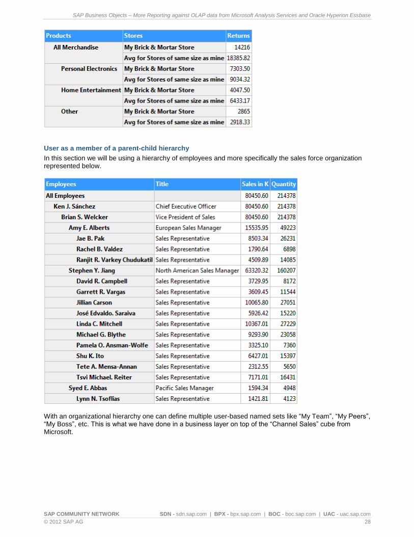
In this section we will be using a hierarchy of employees and more specifically the sales force organization represented below.
With an organizational hierarchy one can define multiple user-based named sets like “My Team”, “My Peers”, “My Boss”, etc. This is what we have done in a business layer on top of the “Channel Sales” cube from Microsoft.

SAP Business Objects – More Reporting against OLAP data from Microsoft Analysis Services and Oracle Hyperion Essbase
SAP COMMUNITY NETWORK SDN - sdn.sap.com | BPX - bpx.sap.com | BOC - boc.sap.com | UAC - uac.sap.com
© 2012 SAP AG 29
The named sets exploit the navigation functions provided by MDX.
Name Expression of the named set
Myself [Employee].[Employees].[@Variable('BOUSER')]
My Direct Reports @Select(Employee\Myself).Item(0).Item(0).Children
My Peers Except( @Select(Employee\Myself).Item(0).Item(0).Siblings , @Select(Employee\Myself) )
My Boss @Select(Employee\Myself).Item(0).Item(0).Parent
My Team Except( Descendants( @Select(Employee\Myself).Item(0).Item(0) ) , @Select(Employee\Myself).Item(0).Item(0) )
Such named sets allow the sales employee to experience a personalized OLAP cube navigation. Additional calculated members will allow him also to evaluate his contribution to the company.
The table below shows how we compute the employee contribution.
Name Expression of the calculated member Solve Order
Format String
My Contribution @Select(Employee\Myself).Item(0).Item(0)
The Company [Employee].[Employees].[All Employees]
My Contribution ratio @Select(Employee\Employees\My Contribution) / @Select(Employee\Employees\The Company)
60 Percent
We gave a solve order of 60 to the contribution ratio so that it takes precedence over the “Sales in K” formula which was assigned a solve order of 20.
Finally we package the three calculated members into a named set called “Contribution”.
SAP Business Objects – More Reporting against OLAP data from Microsoft Analysis Services and Oracle Hyperion Essbase
SAP COMMUNITY NETWORK SDN - sdn.sap.com | BPX - bpx.sap.com | BOC - boc.sap.com | UAC - uac.sap.com
© 2012 SAP AG 30
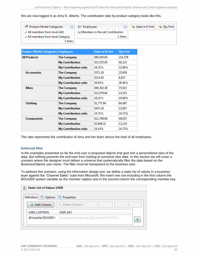
We are now logged in as Amy E. Alberts. The contribution ratio by product category looks like this.
The ratio represents the contribution of Amy and her team versus the total of all employees.
Enforced filter
In the examples presented so far the end-user is proposed objects that give him a personalized view of the data. But nothing prevents the end-user from looking at someone else data. In this section we will cover a scenario where the designer must deliver a universe that systematically filter the data based on the BusinessObjects user name. The filter must be transparent to the business user. To address this scenario, using the information design tool, we define a static list of values in a business layer against the “Channel Sales” cube from Microsoft. We insert one row including in the first column the BOUSER system variable as the member caption and in the second column the corresponding member key.

SAP Business Objects – More Reporting against OLAP data from Microsoft Analysis Services and Oracle Hyperion Essbase
SAP COMMUNITY NETWORK SDN - sdn.sap.com | BPX - bpx.sap.com | BOC - boc.sap.com | UAC - uac.sap.com
© 2012 SAP AG 31
From the properties tab, we specify what the key column is.
We then make the attribute-hierarchy Employee point to the static list of values we have just created.
Let us now define a business filter with the condition: employee equals the system variable obtained from the list of values. We must set the filter as mandatory for all objects in the universe in order to enforce it always.
We are done with setting-up our user-based filter. After testing the universe and before publishing it, we can hide the employee dimension from the end-users with the command: change state to hidden.
SAP Business Objects – More Reporting against OLAP data from Microsoft Analysis Services and Oracle Hyperion Essbase
SAP COMMUNITY NETWORK SDN - sdn.sap.com | BPX - bpx.sap.com | BOC - boc.sap.com | UAC - uac.sap.com
© 2012 SAP AG 32
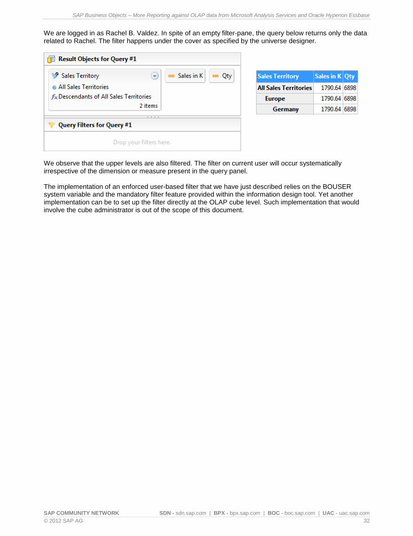
We are logged in as Rachel B. Valdez. In spite of an empty filter-pane, the query below returns only the data related to Rachel. The filter happens under the cover as specified by the universe designer.
We observe that the upper levels are also filtered. The filter on current user will occur systematically irrespective of the dimension or measure present in the query panel. The implementation of an enforced user-based filter that we have just described relies on the BOUSER system variable and the mandatory filter feature provided within the information design tool. Yet another implementation can be to set up the filter directly at the OLAP cube level. Such implementation that would involve the cube administrator is out of the scope of this document.

SAP Business Objects – More Reporting against OLAP data from Microsoft Analysis Services and Oracle Hyperion Essbase
SAP COMMUNITY NETWORK SDN - sdn.sap.com | BPX - bpx.sap.com | BOC - boc.sap.com | UAC - uac.sap.com
© 2012 SAP AG 33
Related Content
Reporting against OLAP Data from Microsoft Analysis Services and Oracle Hyperion Essbase
Profiling and Bucketing dimension members on Microsoft OLAP and Hyperion Essbase
Sample Universe on Microsoft OLAP cube
Create a Relational Connection to SAP HANA
information design tool - eLearning
For more information, visit the Business Objects homepage.
SAP Business Objects – More Reporting against OLAP data from Microsoft Analysis Services and Oracle Hyperion Essbase
SAP COMMUNITY NETWORK SDN - sdn.sap.com | BPX - bpx.sap.com | BOC - boc.sap.com | UAC - uac.sap.com
© 2012 SAP AG 34
Copyright
© Copyright 2012 SAP AG. All rights reserved.
No part of this publication may be reproduced or transmitted in any form or for any purpose without the express permission of SAP AG. The information contained herein may be changed without prior notice.
Some software products marketed by SAP AG and its distributors contain proprietary software components of other software vendors.
Microsoft, Windows, Excel, Outlook, and PowerPoint are registered trademarks of Microsoft Corporation.
IBM, DB2, DB2 Universal Database, System i, System i5, System p, System p5, System x, System z, System z10, System z9, z10, z9, iSeries, pSeries, xSeries, zSeries, eServer, z/VM, z/OS, i5/OS, S/390, OS/390, OS/400, AS/400, S/390 Parallel Enterprise Server, PowerVM, Power Architecture, POWER6+, POWER6, POWER5+, POWER5, POWER, OpenPower, PowerPC, BatchPipes, BladeCenter, System Storage, GPFS, HACMP, RETAIN, DB2 Connect, RACF, Redbooks, OS/2, Parallel Sysplex, MVS/ESA, AIX, Intelligent Miner, WebSphere, Netfinity, Tivoli and Informix are trademarks or registered trademarks of IBM Corporation.
Linux is the registered trademark of Linus Torvalds in the U.S. and other countries.
Adobe, the Adobe logo, Acrobat, PostScript, and Reader are either trademarks or registered trademarks of Adobe Systems Incorporated in the United States and/or other countries.
Oracle is a registered trademark of Oracle Corporation.
UNIX, X/Open, OSF/1, and Motif are registered trademarks of the Open Group.
Citrix, ICA, Program Neighborhood, MetaFrame, WinFrame, VideoFrame, and MultiWin are trademarks or registered trademarks of Citrix Systems, Inc.
HTML, XML, XHTML and W3C are trademarks or registered trademarks of W3C®, World Wide Web Consortium, Massachusetts Institute of Technology.
Java is a registered trademark of Sun Microsystems, Inc.
JavaScript is a registered trademark of Sun Microsystems, Inc., used under license for technology invented and implemented by Netscape.
SAP, R/3, SAP NetWeaver, Duet, PartnerEdge, ByDesign, SAP Business ByDesign, and other SAP products and services mentioned herein as well as their respective logos are trademarks or registered trademarks of SAP AG in Germany and other countries.
Business Objects and the Business Objects logo, BusinessObjects, Crystal Reports, Crystal Decisions, Web Intelligence, Xcelsius, and other Business Objects products and services mentioned herein as well as their respective logos are trademarks or registered trademarks of Business Objects S.A. in the United States and in other countries. Business Objects is an SAP company.
All other product and service names mentioned are the trademarks of their respective companies. Data contained in this document serves informational purposes only. National product specifications may vary.
These materials are subject to change without notice. These materials are provided by SAP AG and its affiliated companies ("SAP Group") for informational purposes only, without representation or warranty of any kind, and SAP Group shall not be liable for errors or omissions with respect to the materials. The only warranties for SAP Group products and services are those that are set forth in the express warranty statements accompanying such products and services, if any. Nothing herein should be construed as constituting an additional warranty.