More Demand / Begin Information

ECO 5550/6550

Fundamental Problems with Demand Estimation for Health Care

• Measuring quantity, price, income.

• Quantity first. It is typically very difficult to define quantity.

• We usually look at the stuff that is easiest to measure. Things like visits, days of service, and the like.

Problems w/ Demand Estimation

• The problem here is that the measures may not be meaningful.

• 5 days of inpatient care for observation is obviously not the same as 5 days of inpatient care for brain surgery.

• We could argue that 5 visits reflects more treatment than 4 visits, but it could simply indicate that the first 4 visits were not effective.

Episodes

• Episodes represent what may be a more theoretically desirable measure of output in a number of ways.

• An episode starts when someone starts to need treatment, and ends when they no longer need it.

• For example, an episode may include a few visits to the doctor, some inpatient hospitalization, and maybe some follow-up clinic visits.

Episodes

• It is usually defined chronologically. In principle, this is the best way to measure both instances of demand, and the costs of treatment.

• Particularly useful, for example, if the make-up of treatment has changed. If, over time, we have substituted outpatient for inpatient care, and we have a few more tests, but they are cheaper, then what is really important is not the number of visits, or the number of days, but the cost of the episode.

Episodes

• These seem great. What are the problems?– They are necessarily arbitrary. We must determine

when the episode starts, and when it ends. Does a certain visit represents more of the same episode, or the beginning of another episode.

– We must look much more carefully into the process that defines the episode, and at behavior within the episode.

– We need complete data on individuals. If individuals go to several providers, or take considerable out-of-plan coverage, it may be very difficult to create episodes with any real confidence.

Example

• Normal delivery of a child.

• Length has changed

• Less days in hospital

• More care at home.

Income

• Most elementally, it is often difficult to find incomes. If we are looking at insurance claims, they often don't have people’s incomes on them.

• Hard to get wage rate to evaluate valuation of time.

• Given that you have income, there are other concerns. Many economists, myself included, feel that many types of expenditures are more appropriately related to long-term, or permanent income, than to measured, or current income. If we try to estimate demand with current income, we get some problems with the demand elasticity.

Price

If we treat coinsurance as simply a fraction, econometrics should not be too difficult.

Rather than measuring price P, we are measuring net price rP. A 10 % change in coinsurance rate is simply the same as a 10 % change in net price.

Insurance is only important IF price is important.

Visits

Mon

ey P

rice Effective P

rice

40

30

20

10 10

20

30

40

Money price demand

Effective demand

Kinks from Insurance3 sections

1. Deductible - same as before

Health Care

Com

posi

te

2. Coinsurance - Other Goods trade off for more health care.

3. Limit - Insurer won't pay more. Back to previous slope.

Budget constraint is now decidedly non-linear, and non-convex

Students tend to fixate on the kinks. May not necessarily be at a kink.

Students tend to fixate on the kinks. May not necessarily be at a kink.

Rand Experiment

• The Rand experimental data randomly assigned people to insurance coverages, thus addressing at least some of the problem.

• Generally these estimates gave coinsurance elasticities of about -0.2. What does this mean?

The Effects of Time and Money Prices on Treatment Attendance

for Methadone Maintenance Clients

Natalia N. BorisovaProcter and Gamble Pharmaceuticals, Cincinnati, Ohio

Allen C. GoodmanWayne State University, Detroit, Michigan

Journal of Substance Abuse Treatment 2004

Methadone treatment

• Methadone maintenance is an unusual and possibly unique health care model.

• First, clients are required to visit a clinic very often (it used to be every day), so treatment attendance becomes essential for clients’ compliance and treatment effectiveness.

• Second, treatment attendance has implications for waste of resources in terms of staff time and the underutilization of equipment.

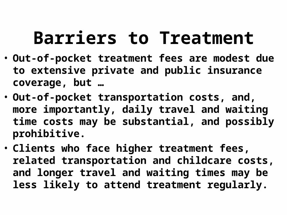
Barriers to Treatment• Out-of-pocket treatment fees are modest due to

extensive private and public insurance coverage, but …

• Out-of-pocket transportation costs, and, more importantly, daily travel and waiting time costs may be substantial, and possibly prohibitive.

• Clients who face higher treatment fees, related transportation and childcare costs, and longer travel and waiting times may be less likely to attend treatment regularly.

Estimating the ModelA = β0 + β1PM + β2PT + β3Y + β4Z + ε (1)

where: PM is the average daily money price; PT is the average daily time price; Y is gross household income; Z is a vector of variables that may influence treatment attendance including socioeconomic and demographicattributes; andε is an error term

Demand v. Willingness to Pay

• Demand – Call out price– Determine quantity

• Willingness to Pay (WTP)– Call out quantity– Determine maximum amount people would

pay.

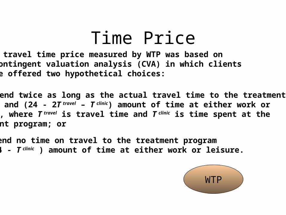
Time PriceThe travel time price measured by WTP was based on a contingent valuation analysis (CVA) in which clients were offered two hypothetical choices:

(1) spend twice as long as the actual travel time to the treatment program and (24 ‑ 2T travel – T clinic) amount of time at either work or leisure, where T travel is travel time and T clinic is time spent at the treatment program; or

(2) spend no time on travel to the treatment program and (24 - T clinic ) amount of time at either work or leisure.

WTP

QuestionsIf you had to pay here for each visit, what is the MOST money you would be willing to pay?

If it took you twice as long as usual to travel to this clinic and if you had to pay, what is the MOST money you would be willing to pay for each visit?

If this clinic were moved right NEXT DOOR to where you live for your convenience and if you had to pay, what is the MOST money you would be willing to pay for each visit?

$10$10

$8$8

$13$13

TT = 40TT = 40

TT = 80TT = 80

TT = 0TT = 0

40 min $2$3/hr.

40 min $2$3/hr.

40 min $3$4.50/hr.

40 min $3$4.50/hr.

WTP, butAlso consistency

WTAccept

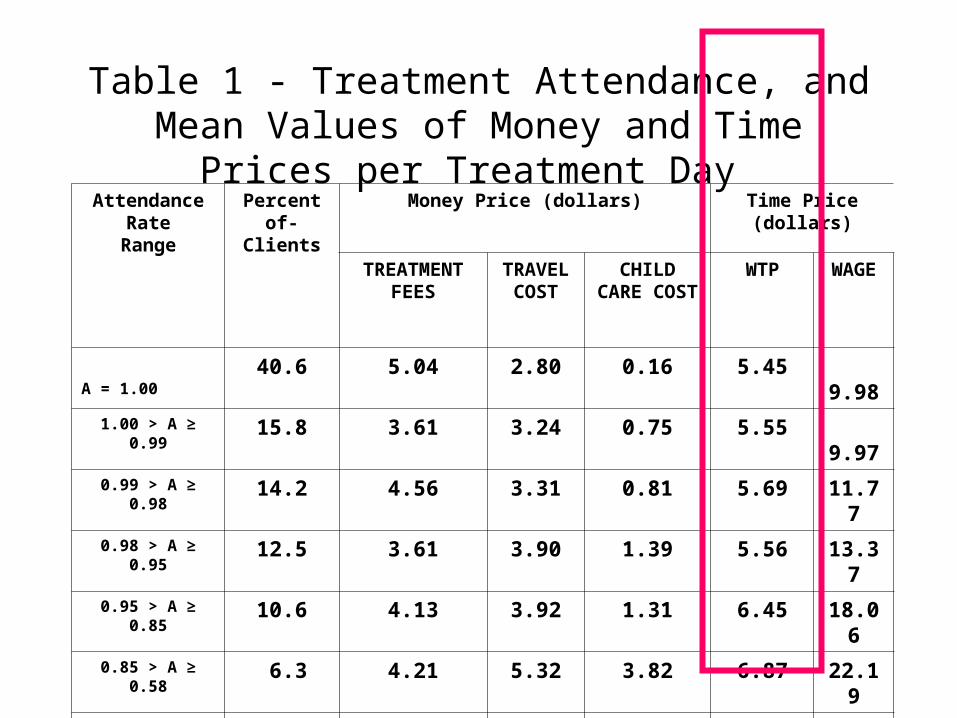
Table 1 - Treatment Attendance, and Mean Values of Money and Time Prices per Treatment Day

Attendance RateRange

Percent of-Clients

Money Price (dollars) Time Price (dollars)

TREATMENT FEES

TRAVEL COST

CHILD CARE COST

WTP WAGE

A = 1.00 40.6 5.04 2.80 0.16 5.45 -9.98

1.00 > A ≥ 0.99 15.8 3.61 3.24 0.75 5.55 -9.97

0.99 > A ≥ 0.98 14.2 4.56 3.31 0.81 5.69 11.77

0.98 > A ≥ 0.95 12.5 3.61 3.90 1.39 5.56 13.37

0.95 > A ≥ 0.85 10.6 4.13 3.92 1.31 6.45 18.06

0.85 > A ≥ 0.58 16.3 4.21 5.32 3.82 6.87 22.19

Total mean - 4.42 3.36 0.85 5.71 12.27

Table 2 – Variable

Definitions and Sample Means

Variables Mean Mean* (A |A<1) Mean (A |A=1)

ATTENDANCE RATE 0.97---- 0.95------ 1.00-------

AFRICAN-AMERICAN 0.33---- 0.44------ 0.17-------

WOMEN 0.47---- 0.48------ 0.45-------

EMPLOYED 0.45---- 0.41------ 0.52-------

MARRIED 0.24---- 0.24------ 0.24-------

AGE 41.80---- 42.05------ 41.43-------

AGE SQUARED 1807.82- 1828.49----- 1777.57-----

CLINIC IN MACOMB COUNTY 0.32---- 0.19------ 0.50-------

CLINIC IN OAKLAND COUNTY 0.33---- 0.31------ 0.36-------

FAMILY INCOME (yearly) 18065. 17853. 18375.

WEEKS IN TREATMENT 80.51---- 83.17------ 76.67-------

NUMBER OF PREVIOUS TREATMENTS 1.00---- 1.19------ 0.72-------

BUS 0.18---- 0.21------ 0.15-------

OTHER TRANSPORTATION 0.02---- 0.02------ 0.01-------

MONEY PRICE ($) per day 8.63---- 9.05------ 8.00-------

TIME PRICE ($) per day, measured by WAGE 12.27---- 13.85------ 9.98-------

TIME PRICE ($) per day, measured by WTP 5.71---- 5.88------ 5.45-------

TRAVEL TIME (in minutes) 81.37---- 91.64------ 66.34-------

WAITING TIME (in minutes) 30.99---- 33.92------ 26.71-------

OBSERVATIONS 303---- 180 123*A is a treatment attendance rate

Variables Parameter T-Ratio η†

A | X Latent A* | X

A | 0.58 < A < 1, X

INTERCEPT 0.9586----- 12.25*** - - -

AFRICAN-AMERICAN -0.0347----- -3.13*** -0.0179 -0.0358 -0.0144

WOMEN -0.0071----- -0.77+++ -0.0036 -0.0073 -0.0029

EMPLOYED 0.0181----- 1.81*++ 0.0093 0.0187 0.0075

MARRIED 0.0082----- 0.77+++ 0.0042 0.0085 0.0034

AGE -6.97E-04---- -0.19+++ 0.0184 0.0367 0.0148

AGE SQUARED 01.84E-05---- 0.41+++ - - -

CLINIC IN MACOMB COUNTY (OUTSIDE CENTRAL CITY)

0.1118----- 7.82*** 0.0577 0.1152 0.0464

CLINIC IN OAKLAND COUNTY (OUTSIDE CENTRAL CITY)

0.0896----- 6.32*** 0.0462 0.0924 0.0372

FAMILY INCOME (per week) -3.4E-05----- -2.06**+ -0.0061 -0.0122 -0.0049

WEEKS IN TREATMENT -5.5E-05----- -1.04+++ -0.0023 -0.0046 -0.0018

PREVIOUS TREATMENT 0.0065----- 1.65*++ 0.0033 0.0067 0.0027

BUS 0.0109----- 0.89+++ 0.0056 0.0112 0.0045

OTHER TRANSPORTATION 0.0354----- 1.03+++ 0.0183 0.0365 0.0147

MONEY PRICE (per week) -1.9E-04----- -1.68*++ -0.0051 -0.0103 -0.0041

TIME PRICE - WTP (per week) -4.2E-04----- -2.84*** -0.0044 -0.0087 -0.0035

OBSERVATIONS 303  

Pr (UNCENSORED) 0.5004  

E (A* | X) 0.9974  

E (A | X) 0.9634  

E (A | 0.58 < A < 1, X) 0.9396  

Table 3Tobit EstimatesUsing WTP

Money price and time price are BOTH important

Money price and time price are BOTH important

Information

Information

• Why do we care?• Problem is asymmetric information.• In many parts of the health care sector,

there are information gaps.• Sometimes the patient knows more than

the provider. Examples? Discuss.• Sometimes the provider knows more than

the patient. Examples? Discuss.

The Lemons Principle

• Shows the problem when we have incomplete information. We will apply this principle DIRECTLY to the purchase of health insurance.

• Key feature these days.

Lemons and Cars

• We have incomplete information on the quality of cars.

• Some may be creampuffs

• Others may be lemons.• What does that do to the

market.• Assume we have 9 cars,

with quality levels varying from 0 to 2.

Probability

0

0.05

0.1

0.15

Quality Level

Probability

Idea

• Owners know how much their cars are worth but potential buyers DON’T.

• Owners know that cars are worth $10,000*Q, where Q is quality.

• Potential buyers are willing to pay $15,000 per unit of quality (they need cars)

• But they only know that the AVERAGE car is worth how much?

• A> $10,000. Why?

Equilibrium price?

• Suppose an auctioneer calls out a price of $20,000 per car. All 9 cars will be offered. Why?

• How many will be bid on?• A> None. Because buyers only know that the mean

quality level is 1 @ a price of $15,000. So you have 9 sellers, no buyers.

Equilibrium price? (2)

• $20,000 doesn’t work.• Suppose auctioneer calls out a price of $15,000 per car.

7 cars will be offered. Why?• The BEST ones are withdrawn since they are worth more

than $15,000.

• Average quality falls from 1 to 0.750. Why?• Potential buyers use price as an indicator of quality, and

recognize that the cars being offered are lower quality. They would only pay $15,000*0.750 = $11,250. Still no bidders. There never will be.

WHY?

• When potential buyers know only the average quality of used cars, then the market prices will tend to be lower than the true value of top quality cars.

• High quality cars are driven out of the market by lemons.

• KEY -- Sellers have information. Buyers DON’T. This is NOT symmetric.

What does information do?

• If both sides have perfect information … all is good. We’ve done enough micro to understand.

• But what if neither side has information?

What if NEITHER has Info?

• Auctioneer starts at $20,000.• Owners guess their cars

have quality level Q = 1.• All 9 cars are offered, but

none are bid.• If price is dropped to

$15,000, all 9 cars are still offered.

• Buyers buy them. • KEY is that the (lack of)

information is symmetric.

Probability

0

0.05

0.1

0.15

Quality Level

Probability

More kinksPrice is correlated with the error

term. Since individuals with large values of the error term are likely to exceed a deductible, and conversely, V will be negative.

That is, a large positive (+) error is correlated with a low price, because after the deductible, we're thrown into a low copayment (and vice versa).

This is noted by error terms in graph. This suggests that the demand curve is more elastic (more negative).