MORE ABOUT HYPOTHESIS TESTING Unit 4A - Statistical Inference Part 1

1

We have now covered the steps in hypothesis testing in general and specifically for the z‐test for one population proportion. 

Now we want to discuss a few issues regarding hypothesis testing which are: 

• The effect of sample size on hypothesis testing

• The difference between statistical significance and practical importance 

• And how hypothesis testing and confidence intervals are related. 

1

1. THE EFFECT OF SAMPLE SIZE ON HYPOTHESIS TESTING

2

We have already seen the effect that the sample size has on inference, when we discussed point and interval estimation for the population mean (μ, mu) and population proportion (p). 

Intuitively …Larger sample sizes give us more information about true nature of the population. We can therefore expect the samplemean and sample proportion obtained from a larger sample to be closer to the population mean and proportion, respectively. 

As a result, for the same level of confidence, we can report a smaller margin of error, and get a narrower confidence interval. 

In hypothesis testing, larger sample sizes have a similar effect. We have also discussed that the power of our test increases when the sample size increases, all else remaining the same. 

This means, we have a better chance to detect the difference between the true value and the null value for larger samples.

The following two examples will illustrate that a larger sample size provides more convincing evidence (the test has greater power), and how the evidence manifests itself in hypothesis testing. 

2

Example 2: Marijuana Use

3

There IS NOT enough evidence that the proportion of students at the college who use marijuana is higher than the national figure.

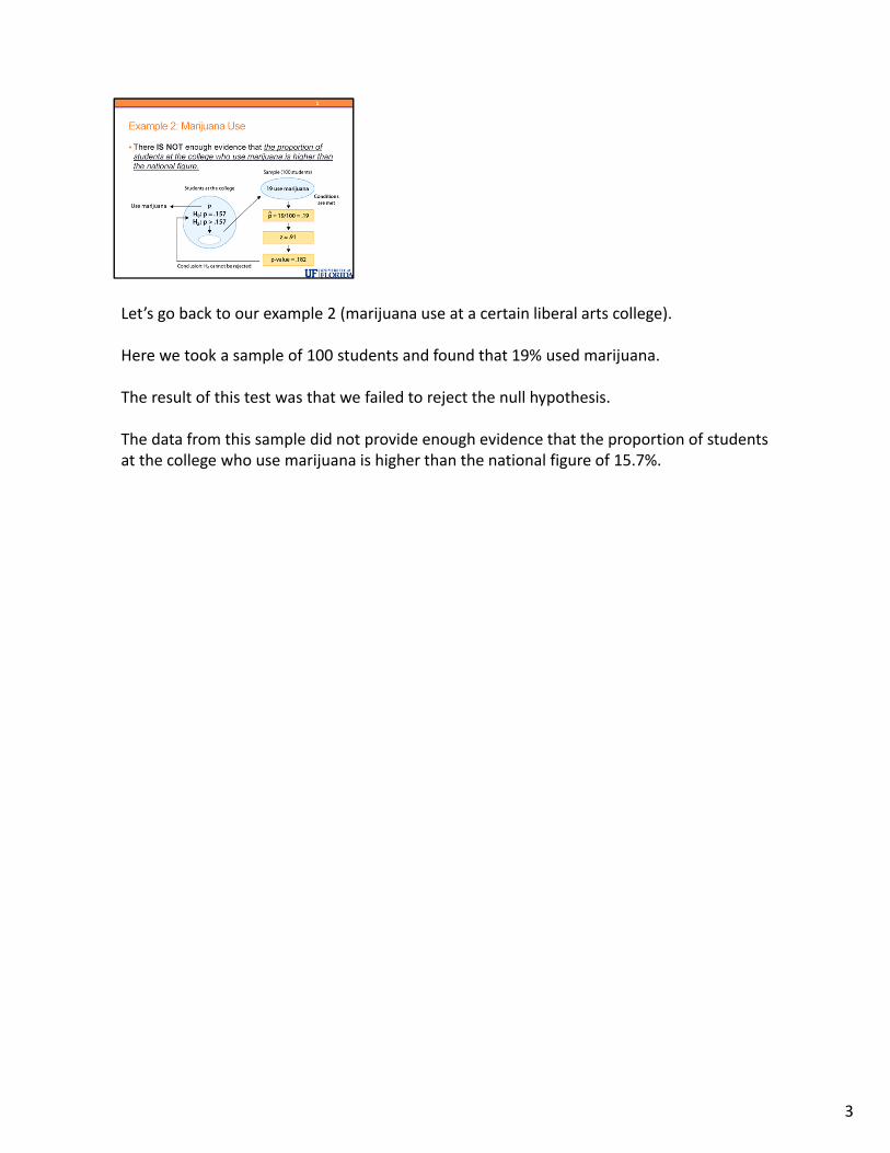
Let’s go back to our example 2 (marijuana use at a certain liberal arts college).

Here we took a sample of 100 students and found that 19% used marijuana. 

The result of this test was that we failed to reject the null hypothesis. 

The data from this sample did not provide enough evidence that the proportion of students at the college who use marijuana is higher than the national figure of 15.7%. 

3

Example: Marijuana Use (LARGER SAMPLE)

4

There IS ENOUGH evidence that the proportion of students at the college who use marijuana is higher than the national figure.

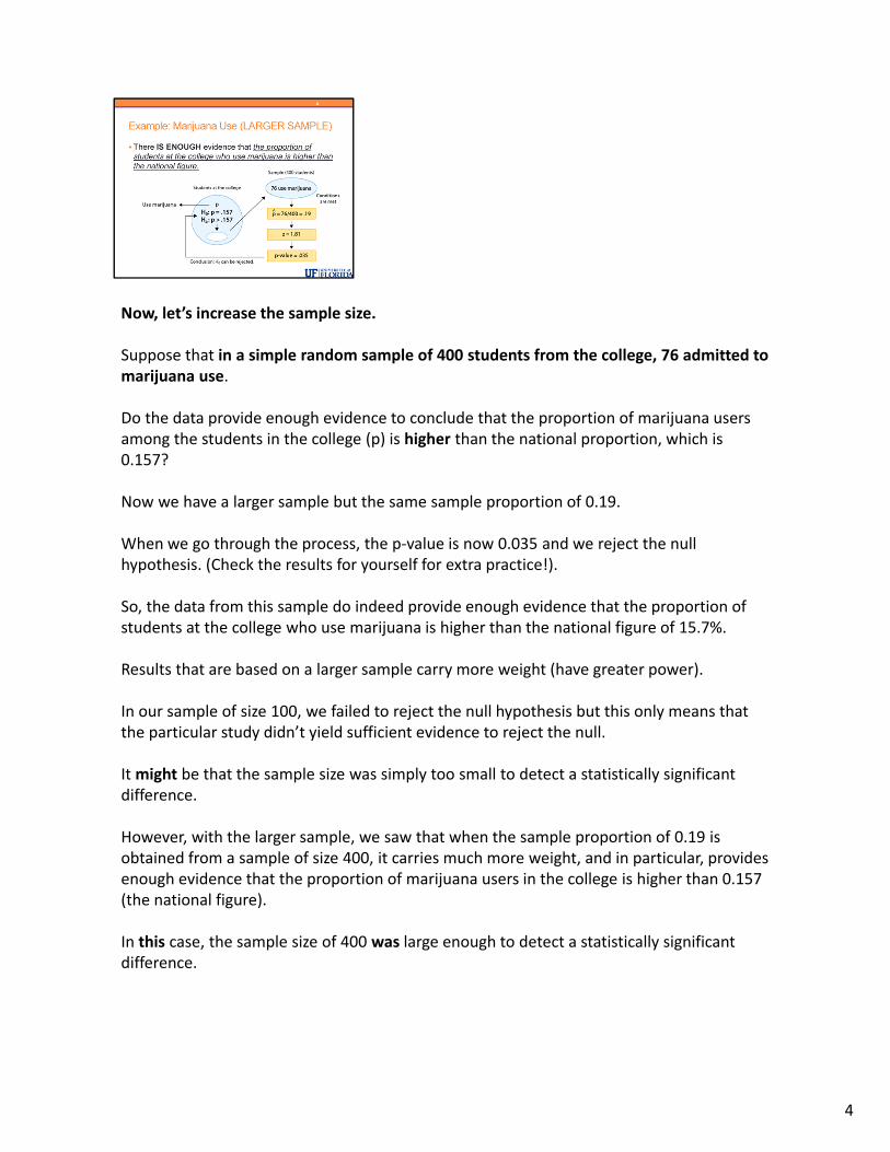
Now, let’s increase the sample size. 

Suppose that in a simple random sample of 400 students from the college, 76 admitted to marijuana use. 

Do the data provide enough evidence to conclude that the proportion of marijuana users among the students in the college (p) is higher than the national proportion, which is 0.157?

Now we have a larger sample but the same sample proportion of 0.19. 

When we go through the process, the p‐value is now 0.035 and we reject the null hypothesis. (Check the results for yourself for extra practice!). 

So, the data from this sample do indeed provide enough evidence that the proportion of students at the college who use marijuana is higher than the national figure of 15.7%. 

Results that are based on a larger sample carry more weight (have greater power).

In our sample of size 100, we failed to reject the null hypothesis but this only means that the particular study didn’t yield sufficient evidence to reject the null. 

Itmight be that the sample size was simply too small to detect a statistically significant difference.

However, with the larger sample, we saw that when the sample proportion of 0.19 is obtained from a sample of size 400, it carries much more weight, and in particular, provides enough evidence that the proportion of marijuana users in the college is higher than 0.157 (the national figure). 

In this case, the sample size of 400 was large enough to detect a statistically significant difference.

4

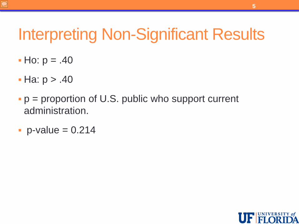
Interpreting Non-Significant Results

Ho: p = .40

Ha: p > .40

p = proportion of U.S. public who support current administration.

p-value = 0.214

5

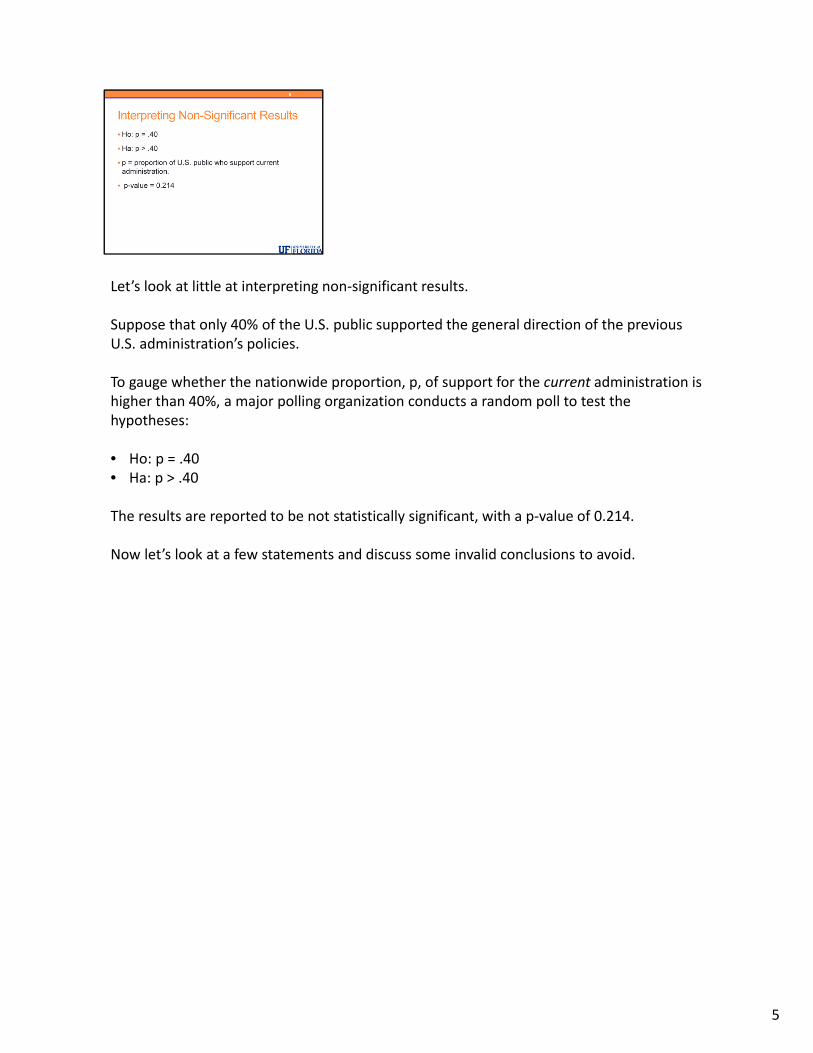
Let’s look at little at interpreting non‐significant results. 

Suppose that only 40% of the U.S. public supported the general direction of the previous U.S. administration’s policies. 

To gauge whether the nationwide proportion, p, of support for the current administration is higher than 40%, a major polling organization conducts a random poll to test the hypotheses:

• Ho: p = .40• Ha: p > .40

The results are reported to be not statistically significant, with a p‐value of 0.214.

Now let’s look at a few statements and discuss some invalid conclusions to avoid. 

5

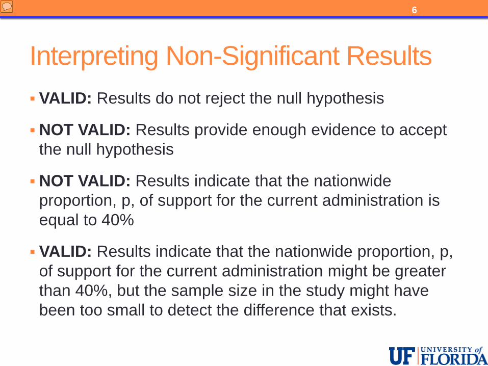
Interpreting Non-Significant Results

VALID: Results do not reject the null hypothesis

NOT VALID: Results provide enough evidence to accept the null hypothesis

NOT VALID: Results indicate that the nationwide proportion, p, of support for the current administration is equal to 40%

VALID: Results indicate that the nationwide proportion, p, of support for the current administration might be greater than 40%, but the sample size in the study might have been too small to detect the difference that exists.

6

There are correct ways to think about results which are not significant and there are a few common misperceptions. 

It is VALID to say: Results do not reject the null hypothesis

It is NOT VALID to say: Results provide enough evidence to accept the null hypothesis

It is NOT VALID to say: Results indicate that the nationwide proportion, p, of support for the current administration is equal to 40%

It is VALID to say: Results indicate that the nationwide proportion, p, of support for the current administration might be greater than 40%, but the sample size in the study might have been too small to detect the difference that exists. 

Remember that in hypothesis testing, failing to reject the null hypothesis does not allow us to say that the null hypothesis is true, only that we do not have enough evidence to reject it. 

6

2. STATISTICAL SIGNIFICANCE VS. PRACTICAL IMPORTANCE.

7

Now, we will address the issue of statistical significance versus practical importance  (sometimes called clinical significance in the health sciences). 

This topic also involves issues of sample size. 

7

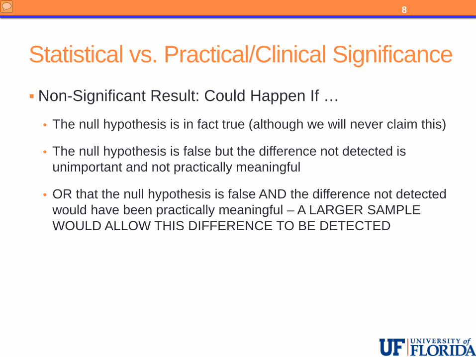
Statistical vs. Practical/Clinical Significance

Non-Significant Result: Could Happen If …

• The null hypothesis is in fact true (although we will never claim this)

• The null hypothesis is false but the difference not detected is unimportant and not practically meaningful

• OR that the null hypothesis is false AND the difference not detected would have been practically meaningful – A LARGER SAMPLE WOULD ALLOW THIS DIFFERENCE TO BE DETECTED

8

We have discussed before the possible reasons for a non‐significant result, here we want to take it a step further.  

• We could have made a correct decision if the null hypothesis is in fact true. 

• The null hypothesis is false but the difference not detected is unimportant and not practically meaningful. 

We have said that the above two cases are in effect both correct decisions in practice as we do not have any interest in detecting unimportant differences. 

• Finally, the null hypothesis is false and the difference we did not detect IS practically important. 

This is a problem, and as we have just discussed it is possible that a non‐significant result may indicate that we need a larger sample size in order to be able to detect a difference of PRACTICAL IMPORTANCE to the researcher. 

This is one extreme, where we find a result which we feel is practically important but we do not find statistical significance with the data at hand. 

8

Statistical vs. Practical/Clinical Significance

Significant Result: Could Happen If …

• The null hypothesis is in fact true but we have made a Type I error (we aren’t interested in this at the moment).

• The null hypothesis is false and the difference we detected is practically meaningful

• OR that the null hypothesis is false but the difference we detected is unimportant and not practically meaningful

• Here we have TOO LARGE of a sample for the question at hand

• WE have found a statistically significant result which has NO PRACTICAL MEANING

9

A Significant Result: Could Happen If …• The null hypothesis is in fact true but we have made a Type I error (we aren’t interested 

in this at the moment).• The null hypothesis is false and the difference we detected is practically meaningful –

This is the perfect scenario. • OR that the null hypothesis is false but the difference we detected is unimportant and 

not practically meaningful • Here we have TOO LARGE of a sample for the question at hand • WE have found a statistically significant result which has NO PRACTICAL 

MEANING

Important Fact: In general, with a sufficiently large sample size you can make any result that has very little practical importance BECOME statistically significant! A large sample size alone does NOT make a “good” study!!

9

IMPORTANT FACT

When interpreting results of a test,

ALWAYS think not only about

STATISTICAL SIGNIFICANCE of

the results but also about their

PRACTICAL IMPORTANCE

10

This suggests that when interpreting the results of a test, you should always think not only about the statistical significance of the results but also about their practical importance.

10

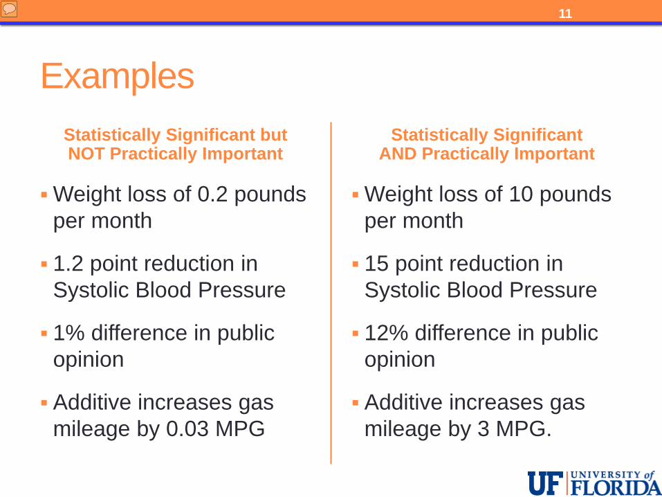
Examples

Statistically Significant but NOT Practically Important

Weight loss of 0.2 pounds per month

1.2 point reduction in Systolic Blood Pressure

1% difference in public opinion

Additive increases gas mileage by 0.03 MPG

Statistically Significant AND Practically Important

Weight loss of 10 pounds per month

15 point reduction in Systolic Blood Pressure

12% difference in public opinion

Additive increases gas mileage by 3 MPG.

11

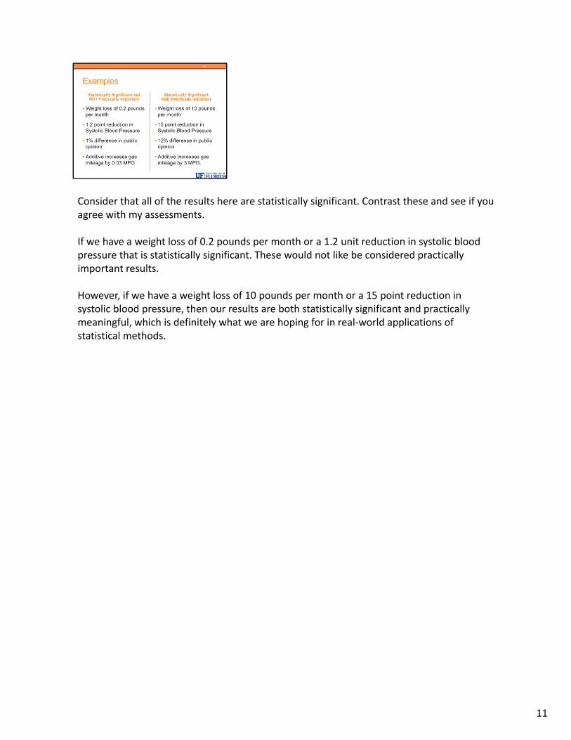
Consider that all of the results here are statistically significant. Contrast these and see if you agree with my assessments.

If we have a weight loss of 0.2 pounds per month or a 1.2 unit reduction in systolic blood pressure that is statistically significant. These would not like be considered practically important results. 

However, if we have a weight loss of 10 pounds per month or a 15 point reduction in systolic blood pressure, then our results are both statistically significant and practically meaningful, which is definitely what we are hoping for in real‐world applications of statistical methods. 

11

3. HYPOTHESIS TESTING AND CONFIDENCE INTERVALS

12

The last topic we want to discuss is the relationship between hypothesis testing and confidence intervals. 

Even though the purpose of these two forms of inference is different (confidence intervals estimate a parameter, and hypothesis testing assesses the evidence in the data against one claim and in favor of another), there is a strong link between them.

We will explain this link (using the z‐test and confidence interval for the population proportion), and then explain how confidence intervals can be used after a test has been carried out.

12

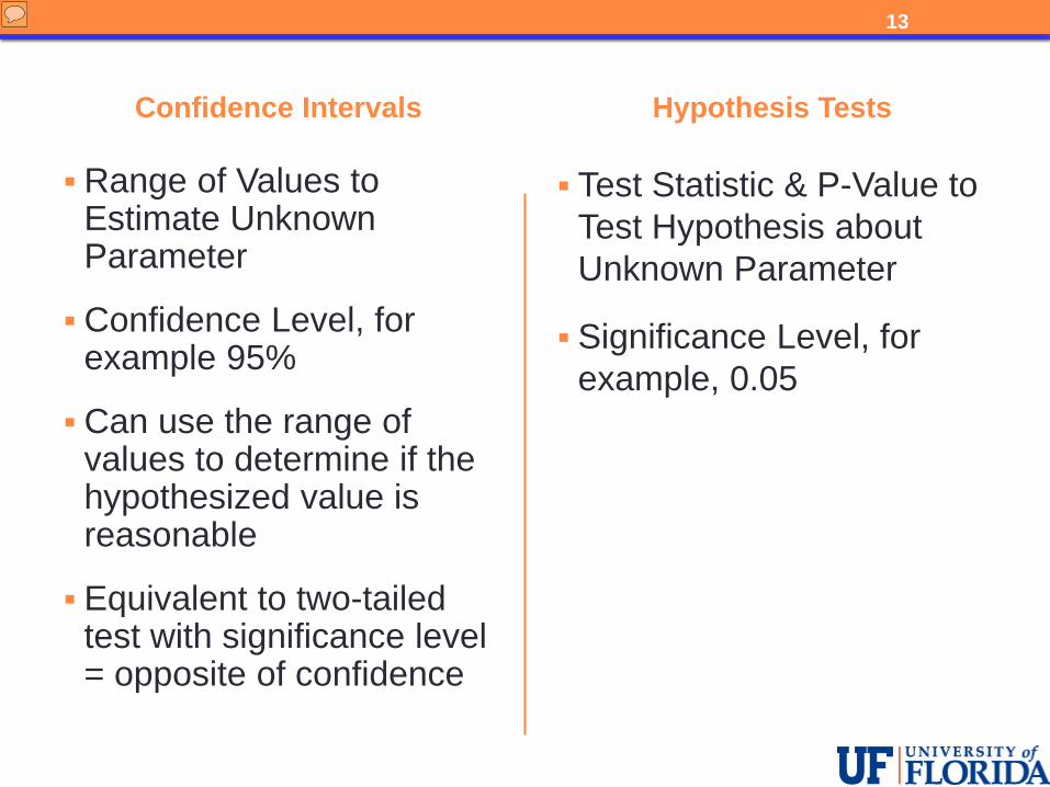
Confidence Intervals

Range of Values to Estimate Unknown Parameter

Confidence Level, for example 95%

Can use the range of values to determine if the hypothesized value is reasonable

Equivalent to two-tailed test with significance level = opposite of confidence

Hypothesis Tests

Test Statistic & P-Value to Test Hypothesis about Unknown Parameter

Significance Level, for example, 0.05

13

Recall that a confidence interval gives us a set of plausible values for the unknown population parameter. 

So, we can examine a confidence interval to decide if a proposed value of population proportion seems plausible.

Confidence intervals are based upon the chance they are correct in the long run – the confidence level. 

Where hypothesis tests are based upon the chance they are incorrect in the long run (via a Type I error) using a significance level. 

The two‐sided hypothesis test with a 5% significance level corresponds directly to the 95% confidence interval and we can use the confidence interval to determine whether to reject the null hypothesis or not based upon whether the null value falls outside the interval or not. 

There are one‐sided confidence intervals which are equivalent to the one‐sided tests but they are rarely used and we will not discuss them in this course. 

13

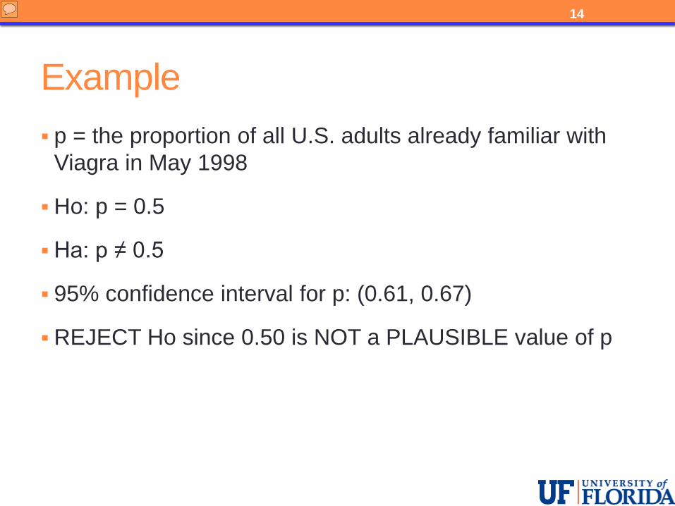
Example

p = the proportion of all U.S. adults already familiar with Viagra in May 1998

Ho: p = 0.5

Ha: p ≠ 0.5

95% confidence interval for p: (0.61, 0.67)

REJECT Ho since 0.50 is NOT a PLAUSIBLE value of p

14

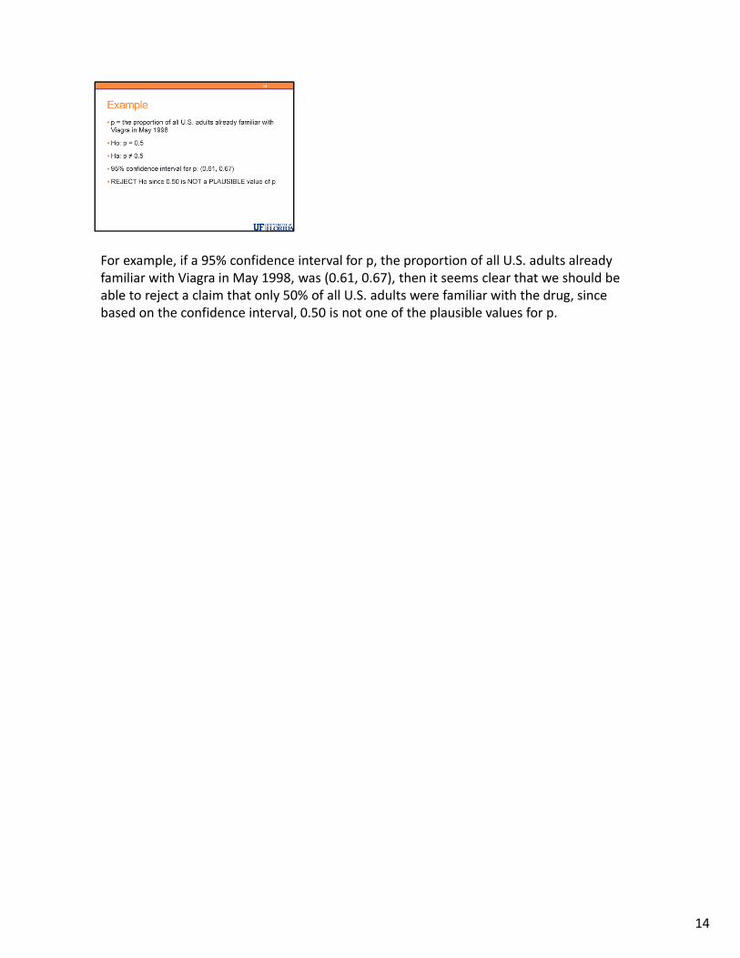
For example, if a 95% confidence interval for p, the proportion of all U.S. adults already familiar with Viagra in May 1998, was (0.61, 0.67), then it seems clear that we should be able to reject a claim that only 50% of all U.S. adults were familiar with the drug, since based on the confidence interval, 0.50 is not one of the plausible values for p.

14

Conduct Test: Confidence Intervals

Ho: p = p0

Ha: p ≠ p0

Find a 95% confidence interval for p and check:

If p0 falls outside the confidence interval, reject Ho.

• Here p0 is not one of the plausible values for p

If p0 falls inside the confidence interval, do not reject Ho.

• Here p0 is one of the plausible values for p

15

Suppose we want to carry out the two‐sided test:• Ho: p = p0• Ha: p ≠ p0using a significance level of 0.05.

We can use the 95% confidence interval for p to conduct this test by checking to see if • If p0 falls outside the confidence interval, then we reject Ho.• If p0 falls inside the confidence interval, then we do not reject Ho.

In other words, • If p0 is not one of the plausible values for p, we reject Ho.• If p0 is a plausible value for p, we cannot reject Ho.

Similarly, the results of a test using a significance level of 0.01 can be related to the 99% confidence interval, and so on. 

15

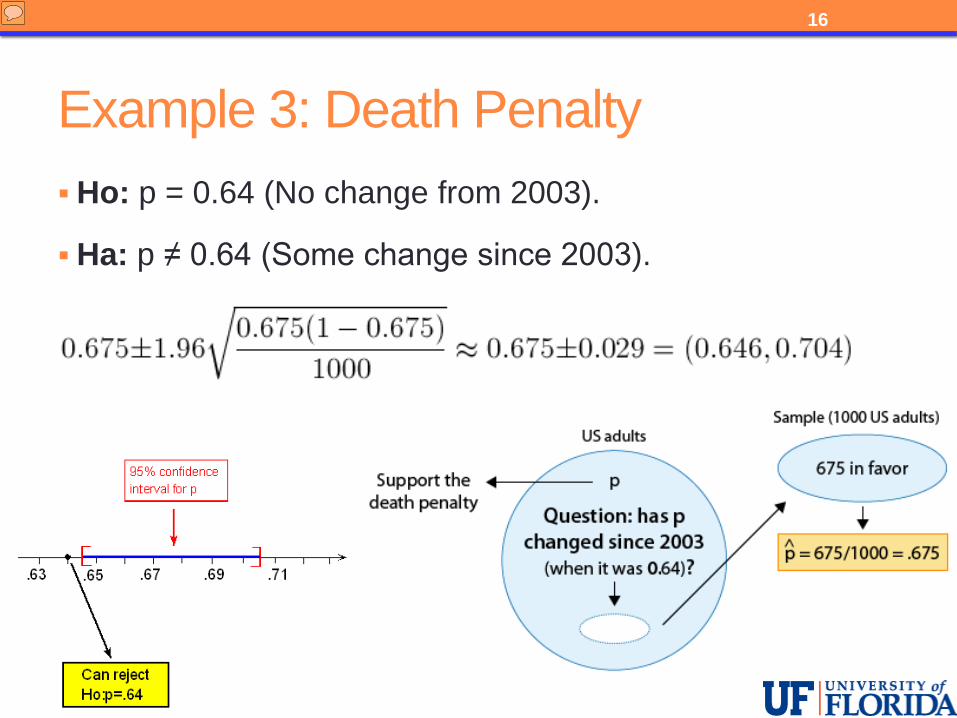
Example 3: Death Penalty

Ho: p = 0.64 (No change from 2003).

Ha: p ≠ 0.64 (Some change since 2003).

16

In example 3, we wanted to know whether the proportion of U.S. adults who support the death penalty for convicted murderers has changed since 2003, when it was 0.64.

We are testing:• Ho: p = 0.64 (No change from 2003).• Ha: p ≠ 0.64 (Some change since 2003).

The 95% confidence interval for p, the proportion of all U.S. adults who support the death penalty, is: (0.646, 0.704). 

Since the 95% confidence interval for p does not include 0.64 as a plausible value for p, we can reject Ho and conclude (as we did before) that the proportion of U.S. adults who support the death penalty for convicted murderers has changed since 2003.

16

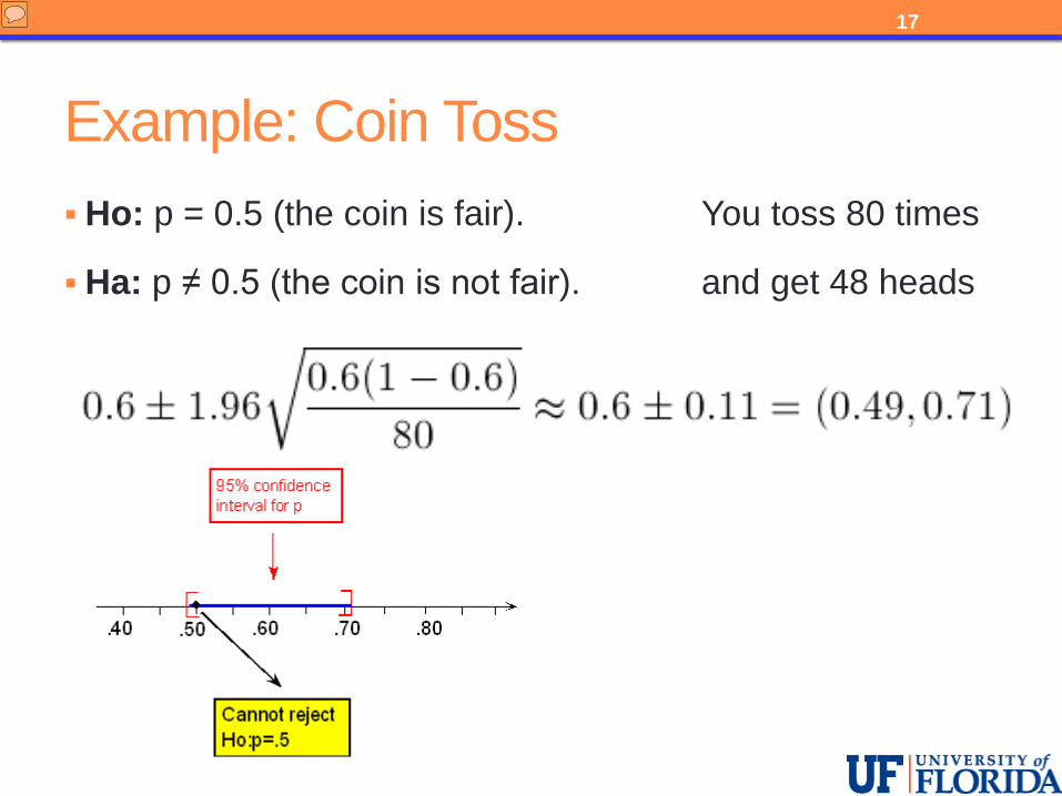
Example: Coin Toss

Ho: p = 0.5 (the coin is fair). You toss 80 times

Ha: p ≠ 0.5 (the coin is not fair). and get 48 heads

17

• You and your roommate are arguing about whose turn it is to clean the apartment. Your roommate suggests that you settle this by tossing a coin and takes one out of a locked box he has on the shelf. 

• Suspecting that the coin might not be fair, you decide to test it first. You toss the coin 80 times, thinking to yourself that if, indeed, the coin is fair, you should get around 40 heads. Instead you get 48 heads. 

• You are not sure whether getting 48 heads out of 80 is enough evidence to conclude that the coin is unbalanced, or whether this a result that could have happened just by chance when the coin is fair.

Let p be the true proportion (probability) of heads. We want to test whether the coin is fair or not.• Ho: p = 0.5 (the coin is fair).• Ha: p ≠ 0.5 (the coin is not fair).The data we have are that out of n = 80 tosses, we got 48 heads, or that the sample proportion of heads is p‐hat = 48/80 = 0.6.• A 95% confidence interval for p, the true proportion of heads for this coin, is: (0.49, 0.71). • Since in this case 0.5 is one of the plausible values for p, we cannot reject Ho. In other 

words, the data do not provide enough evidence to conclude that the coin is not fair.• The context of this example is a good opportunity to bring up an important point that was 

discussed earlier.• Even though we use 0.05 as a cutoff to guide our decision about whether the results are 

significant, we should not treat it as a magic number and we should always add our own judgment. Let’s look at the last example again.

• It turns out that the p‐value of this test is 0.0734. In other words, it is maybe not extremely unlikely, but it is quite unlikely (probability of 0.0734) that when you toss a fair coin 80 times you’ll get a sample proportion of heads of 48/80 = 0.6 (or even more extreme). 

• It is true that using the 0.05 significance level (cutoff), 0.0734 is not considered small enough to conclude that the coin is not fair. 

• However, if you really don’t want to clean the apartment, the p‐value might be small enough for you to ask your roommate to use a different coin, or to provide one yourself.

17

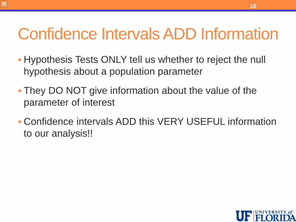
Confidence Intervals ADD Information

Hypothesis Tests ONLY tell us whether to reject the null hypothesis about a population parameter

They DO NOT give information about the value of the parameter of interest

Confidence intervals ADD this VERY USEFUL information to our analysis!!

18

Confidence intervals provide additional information that hypothesis tests do not provide. 

Hypothesis tests ONLY tell us whether to reject the null hypothesis about a population parameter

Hypothesis tests DO NOT give information about the value of the parameter of interest

Confidence intervals ADD this VERY USEFUL information to our analysis!! 

18

Example 3: Death Penalty

The data provide evidence that the proportion of U.S. adults who support the death penalty for convicted murderers has changed since 2003, and we are 95% confident that it is now between 0.646 and 0.704. (i.e. between 64.6% and 70.4%).

19

In Example 3, we concluded that the proportion of U.S. adults who support the death penalty for convicted murderers has changed since 2003, when it was 0.64. 

We’ve calculated the 95% confidence interval for p and found that it is (0.646, 0.704).

Combining this information we can say that the data provide evidence that the proportion of U.S. adults who support the death penalty for convicted murderers has changed since 2003, and we are 95% confident that it is now between 0.646 and 0.704. (i.e. between 64.6% and 70.4%).

19

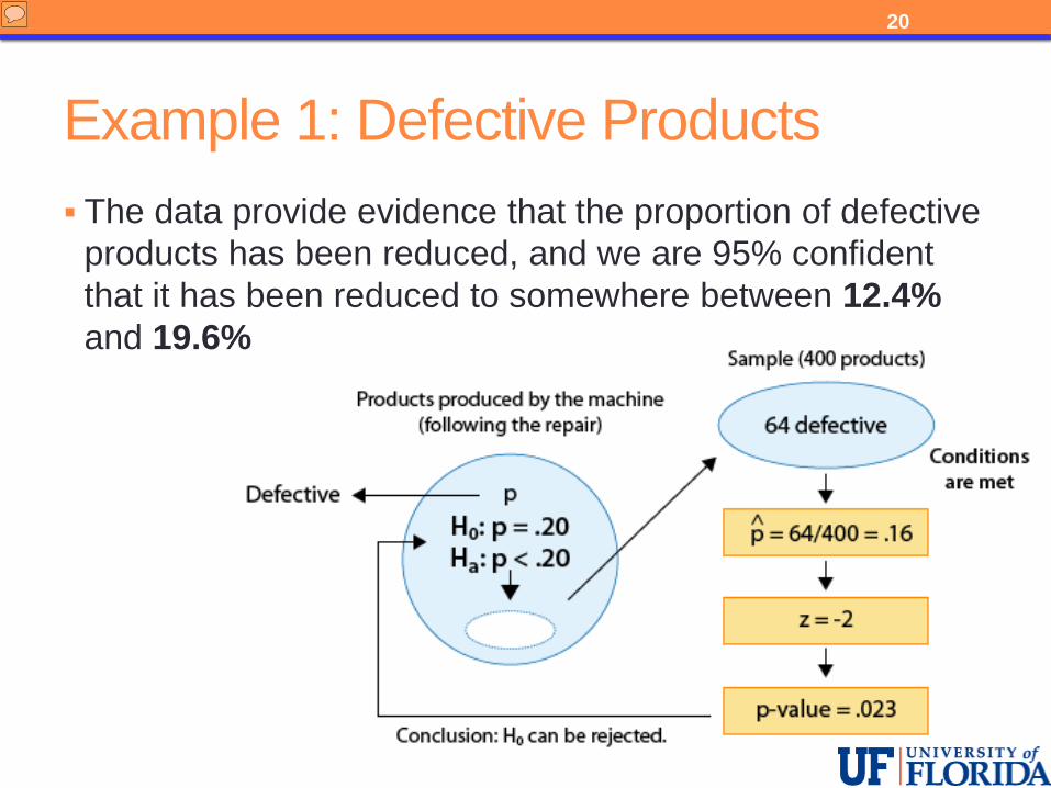
Example 1: Defective Products

The data provide evidence that the proportion of defective products has been reduced, and we are 95% confident that it has been reduced to somewhere between 12.4% and 19.6%

20

We concluded that as a result of the repair, the proportion of defective products has been reduced to below 0.20 (which was the proportion prior to the repair). 

It is probably of great interest to the company not only to know that the proportion of defective items has been reduced, but also estimate what it is now, to get a better sense of how effective the repair was. A 95% confidence interval for p in this case is (0.124, 0.196)

We can therefore say that the data provide evidence that the proportion of defective products has been reduced, and we are 95% confident that it has been reduced to somewhere between 12.4% and 19.6%. 

This is very useful information, since it tells us that even though the results were significant (i.e., the repair reduced the number of defective products), the repair might not have been effective enough, if it managed to reduce the number of defective products only to the range provided by the confidence interval. 

This, of course, ties back in to the idea of statistical significance vs. practical importance that we discussed earlier. Even though the results are statistically significant (Ho was rejected), practically speaking, the repair might still be considered ineffective.

20

MORE ABOUT HYPOTHESIS TESTING

21

We have now covered the general steps for hypothesis tests and some more difficult concepts such as Type I error, Type II error, and Power. 

We have looked at working through the process by hand for the specific example of the z‐test for one population proportion.

And now we have discussed a number of important issues that relate to hypothesis testing in general. 

• The effect of sample size on hypothesis tests• The idea of statistical significance vs. practical importance• The connection between confidence intervals and hypothesis tests• The usefulness of confidence intervals as an addition to the results of a hypothesis test

These ideas will repeat for all of the tests we will learn during the last unit of this course as well as to any tests you learn in the future. 

You will likely need to review all of this material on Hypothesis Testing in Unit 4A more than once to gain a full understanding. 

21