Embed Size (px)
Citation preview
MOPEC: multiple optimization problems withequilibrium constraints
Michael C. Ferris
Joint work with: Michael Bussieck, Steven Dirkse, Jan Jagla andAlexander Meeraus
Supported partly by AFOSR, DOE and NSF
University of Wisconsin, Madison
MOPTA, Lehigh UniversityAugust 18, 2011
Ferris (Univ. Wisconsin) EMP MOPTA 2011 1 / 27
Optimization beyond our discipline
So you can solve an LP, MIP, NLP, SOCP, SDP, MCP, SPI N times fasterI M times largerI or with K times better optimality guarantee
than at MOPTA 2010
Why aren’t you using my *********** algorithm?(Michael Ferris, Boulder, CO, 1994)
Should I care?
Does it make a difference (how large is K, M or N)?
Just solving a single problem isn’t the real value of optimizationI (Ceria): optimization finds “holes” in the model
Optimization is part of a larger processI (Stein): use dual to allow online solution of primalI (Zhu/Chen): solve SDP relaxations
Ferris (Univ. Wisconsin) EMP MOPTA 2011 2 / 27
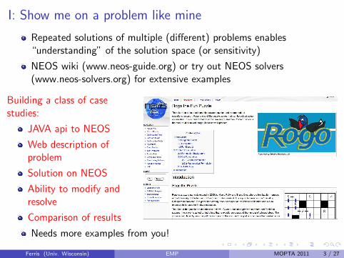
I: Show me on a problem like mine
Repeated solutions of multiple (different) problems enables“understanding” of the solution space (or sensitivity)
NEOS wiki (www.neos-guide.org) or try out NEOS solvers(www.neos-solvers.org) for extensive examples
Building a class of casestudies:
JAVA api to NEOS
Web description ofproblem
Solution on NEOS
Ability to modify andresolve
Comparison of results
Needs more examples from you!
Ferris (Univ. Wisconsin) EMP MOPTA 2011 3 / 27
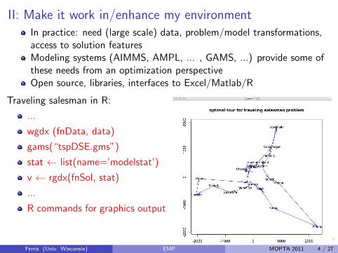
II: Make it work in/enhance my environmentIn practice: need (large scale) data, problem/model transformations,access to solution featuresModeling systems (AIMMS, AMPL, ... , GAMS, ...) provide some ofthese needs from an optimization perspectiveOpen source, libraries, interfaces to Excel/Matlab/R
Traveling salesman in R:
...
wgdx (fnData, data)
gams(“tspDSE.gms”)
stat ← list(name=’modelstat’)
v ← rgdx(fnSol, stat)
...
R commands for graphics output
Ferris (Univ. Wisconsin) EMP MOPTA 2011 4 / 27
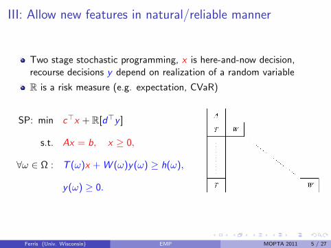
III: Allow new features in natural/reliable manner
Two stage stochastic programming, x is here-and-now decision,recourse decisions y depend on realization of a random variable
R is a risk measure (e.g. expectation, CVaR)
SP: min c>x + R[d>y ]
s.t. Ax = b, x ≥ 0,
∀ω ∈ Ω : T (ω)x + W (ω)y(ω) ≥ h(ω),
y(ω) ≥ 0.
A
T W
T
igure Constraints matrix structure of 15)
problem by suitable subgradient methods in an outer loop. In the inner loop, the second-stage problem is solved for various r i g h t h a n d sides. Convexity of the master is inherited from the convexity of the value function in linear programming. In dual decomposition, (Mulvey and Ruszczyhski 1995, Rockafellar and Wets 1991), a convex non-smooth function of Lagrange multipliers is minimized in an outer loop. Here, convexity is granted by fairly general reasons that would also apply with integer variables in 15). In the inner loop, subproblems differing only in their r i g h t h a n d sides are to be solved. Linear (or convex) programming duality is the driving force behind this procedure that is mainly applied in the multi-stage setting.
When following the idea of primal decomposition in the presence of integer variables one faces discontinuity of the master in the outer loop. This is caused by the fact that the value function of an MILP is merely lower semicontinuous in general Computations have to overcome the difficulty of lower semicontinuous minimization for which no efficient methods exist up to now. In Car0e and Tind (1998) this is analyzed in more detail. In the inner loop, MILPs arise which differ in their r i g h t h a n d sides only. Application of Gröbner bases methods from computational algebra has led to first computational techniques that exploit this similarity in case of pure-integer second-stage problems, see Schultz, Stougie, and Van der Vlerk (1998).
With integer variables, dual decomposition runs into trouble due to duality gaps that typically arise in integer optimization. In L0kketangen and Woodruff (1996) and Takriti, Birge, and Long (1994, 1996), Lagrange multipliers are iterated along the lines of the progressive hedging algorithm in Rockafellar and Wets (1991) whose convergence proof needs continuous variables in the original problem. Despite this lack of theoretical underpinning the computational results in L0kketangen and Woodruff (1996) and Takriti, Birge, and Long (1994 1996), indicate that for practical problems acceptable solutions can be found this way. A branch-and-bound method for stochastic integer programs that utilizes stochastic bounding procedures was derived in Ruszczyriski, Ermoliev, and Norkin (1994). In Car0e and Schultz (1997) a dual decomposition method was developed that combines Lagrangian relaxation of non-anticipativity constraints with branch-and-bound. We will apply this method to the model from Section and describe the main features in the remainder of the present section.
The idea of scenario decomposition is well known from stochastic programming with continuous variables where it is mainly used in the mul t i s tage case. For stochastic integer programs scenario decomposition is advantageous already in the two-stage case. The idea is
Ferris (Univ. Wisconsin) EMP MOPTA 2011 5 / 27
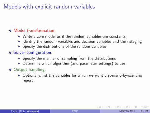
Models with explicit random variables
Model transformation:I Write a core model as if the random variables are constantsI Identify the random variables and decision variables and their stagingI Specify the distributions of the random variables
Solver configuration:I Specify the manner of sampling from the distributionsI Determine which algorithm (and parameter settings) to use
Output handling:I Optionally, list the variables for which we want a scenario-by-scenario
report
Ferris (Univ. Wisconsin) EMP MOPTA 2011 6 / 27
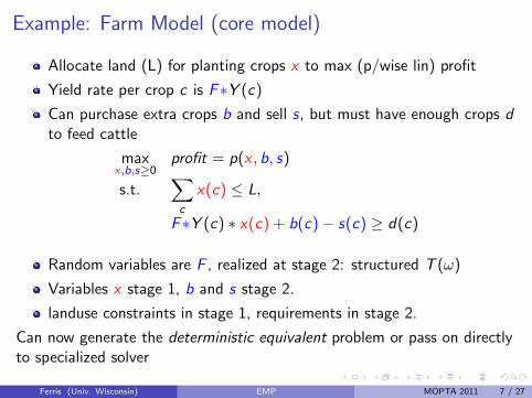
Example: Farm Model (core model)
Allocate land (L) for planting crops x to max (p/wise lin) profit
Yield rate per crop c is F∗Y (c)
Can purchase extra crops b and sell s, but must have enough crops dto feed cattle
maxx ,b,s≥0
profit = p(x , b, s)
s.t.∑c
x(c) ≤ L,
F∗Y (c) ∗ x(c) + b(c)− s(c) ≥ d(c)
Random variables are F , realized at stage 2: structured T (ω)
Variables x stage 1, b and s stage 2.
landuse constraints in stage 1, requirements in stage 2.
Can now generate the deterministic equivalent problem or pass on directlyto specialized solver
Ferris (Univ. Wisconsin) EMP MOPTA 2011 7 / 27
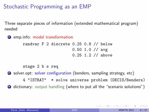
Stochastic Programming as an EMP
Three separate pieces of information (extended mathematical program)needed
1 emp.info: model transformation
randvar F 2 discrete 0.25 0.8 // below
0.50 1.0 // avg
0.25 1.2 // above
stage 2 b s req
2 solver.opt: solver configuration (benders, sampling strategy, etc)
4 "ISTRAT" * solve universe problem (DECIS/Benders)
3 dictionary: output handling (where to put all the “scenario solutions”)
Ferris (Univ. Wisconsin) EMP MOPTA 2011 8 / 27
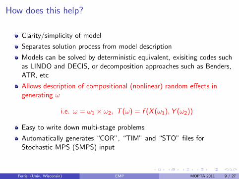
How does this help?
Clarity/simplicity of model
Separates solution process from model description
Models can be solved by deterministic equivalent, exisiting codes suchas LINDO and DECIS, or decomposition approaches such as Benders,ATR, etc
Allows description of compositional (nonlinear) random effects ingenerating ω
i.e. ω = ω1 × ω2, T (ω) = f (X (ω1),Y (ω2))
Easy to write down multi-stage problems
Automatically generates “COR”, “TIM” and “STO” files forStochastic MPS (SMPS) input
Ferris (Univ. Wisconsin) EMP MOPTA 2011 9 / 27
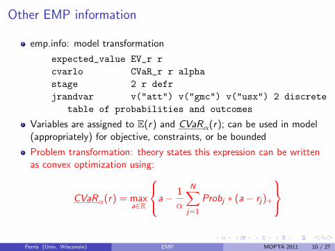
Other EMP information
emp.info: model transformation
expected_value EV_r r
cvarlo CVaR_r r alpha
stage 2 r defr
jrandvar v("att") v("gmc") v("usx") 2 discrete
table of probabilities and outcomes
Variables are assigned to E(r) and CVaRα(r); can be used in model(appropriately) for objective, constraints, or be bounded
Problem transformation: theory states this expression can be writtenas convex optimization using:
CVaRα(r) = maxa∈R
a− 1
α
N∑j=1
Probj ∗ (a− rj)+
Ferris (Univ. Wisconsin) EMP MOPTA 2011 10 / 27
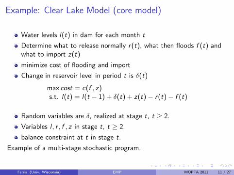
Example: Clear Lake Model (core model)
Water levels l(t) in dam for each month t
Determine what to release normally r(t), what then floods f (t) andwhat to import z(t)
minimize cost of flooding and import
Change in reservoir level in period t is δ(t)
max cost = c(f , z)s.t. l(t) = l(t − 1) + δ(t) + z(t)− r(t)− f (t)
Random variables are δ, realized at stage t, t ≥ 2.
Variables l , r , f , z in stage t, t ≥ 2.
balance constraint at t in stage t.
Example of a multi-stage stochastic program.
Ferris (Univ. Wisconsin) EMP MOPTA 2011 11 / 27
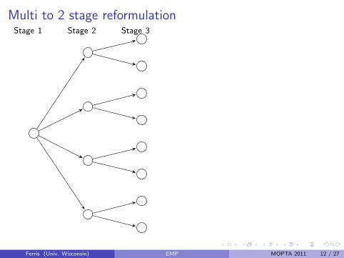
Multi to 2 stage reformulationStage 1 Stage 2 Stage 3
Cut at stage 2
Cut at stage 3
Ferris (Univ. Wisconsin) EMP MOPTA 2011 12 / 27

Multi to 2 stage reformulationStage 1 Stage 2 Stage 3
Cut at stage 2
Cut at stage 3
Ferris (Univ. Wisconsin) EMP MOPTA 2011 12 / 27

Multi to 2 stage reformulationStage 1 Stage 2 Stage 3
Cut at stage 2
Cut at stage 3
Ferris (Univ. Wisconsin) EMP MOPTA 2011 12 / 27
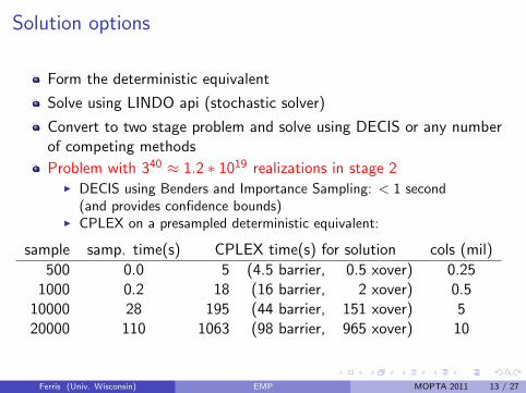
Solution options
Form the deterministic equivalent
Solve using LINDO api (stochastic solver)
Convert to two stage problem and solve using DECIS or any numberof competing methods
Problem with 340 ≈ 1.2 ∗ 1019 realizations in stage 2I DECIS using Benders and Importance Sampling: < 1 second
(and provides confidence bounds)I CPLEX on a presampled deterministic equivalent:
sample samp. time(s) CPLEX time(s) for solution cols (mil)
500 0.0 5 (4.5 barrier, 0.5 xover) 0.251000 0.2 18 (16 barrier, 2 xover) 0.5
10000 28 195 (44 barrier, 151 xover) 520000 110 1063 (98 barrier, 965 xover) 10
Ferris (Univ. Wisconsin) EMP MOPTA 2011 13 / 27
IV: Build coupled/structured models that engage thedecision maker
The next generation electric grid will be more dynamic, flexible,constrained, and more complicated.
Decision processes (in this environment) are predominantlyhierarchical.
Models to support such decision processes must also be layered orhierachical.
Optimization and computation facilitate adaptivity, control, treatmentof uncertainties and understanding of interaction effects.
Developing interfaces and exploiting hierarchical structure usingcomputationally tractable algorithms will provide overall solutionspeed, understanding of localized effects, and value for the couplingof the system.
Ferris (Univ. Wisconsin) EMP MOPTA 2011 14 / 27
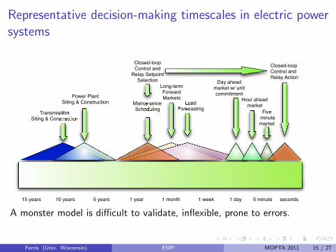
Representative decision-making timescales in electric powersystems
15 years 10 years 5 years 1 year 1 month 1 week 1 day 5 minute seconds
TransmissionSiting & Construction
Power PlantSiting & Construction Maintenance
Scheduling
Long-termForwardMarkets
LoadForecasting
Closed-loopControl and Relay Action
Closed-loopControl and
Relay SetpointSelection Day ahead
market w/ unit commitment
Hour aheadmarket
Five minutemarket
Figure 1: Representative decision-making timescales in electric power systems
environment presents. As an example of coupling of decisions across time scales, consider decisionsrelated to the siting of major interstate transmission lines. One of the goals in the expansion ofnational-scale transmission infrastructure is that of enhancing grid reliability, to lessen our nation’sexposure to the major blackouts typified by the eastern U.S. outage of 2003, and Western Areaoutages of 1996. Characterizing the sequence of events that determines whether or not a particularindividual equipment failure cascades to a major blackout is an extremely challenging analysis.Current practice is to use large numbers of simulations of power grid dynamics on millisecond tominutes time scales, and is influenced by such decisions as settings of protective relays that removelines and generators from service when operating thresholds are exceeded. As described below, weintend to build on our previous work to cast this as a phase transition problem, where optimizationtools can be applied to characterize resilience in a meaningful way.
In addition to this coupling across time scales, one has the challenge of structural differencesamongst classes of decision makers and their goals. At the longest time frame, it is often theIndependent System Operator, in collaboration with Regional Transmission Organizations andregulatory agencies, that are charged with the transmission design and siting decisions. Thesedecisions are in the hands of regulated monopolies and their regulator. From the next longesttime frame through the middle time frame, the decisions are dominated by capital investment andmarket decisions made by for-profit, competitive generation owners. At the shortest time frames,key decisions fall back into the hands of the Independent System Operator, the entity typicallycharged with balancing markets at the shortest time scale (e.g., day-ahead to 5-minute ahead), andwith making any out-of-market corrections to maintain reliable operation in real time. In short,there is clearly a need for optimization tools that effectively inform and integrate decisions acrosswidely separated time scales and who have differing individual objectives.
The purpose of the electric power industry is to generate and transport electric energy toconsumers. At time frames beyond those of electromechanical transients (i.e. beyond perhaps, 10’sof seconds), the core of almost all power system representations is a set of equilibrium equationsknown as the power flow model. This set of nonlinear equations relates bus (nodal) voltagesto the flow of active and reactive power through the network and to power injections into thenetwork. With specified load (consumer) active and reactive powers, generator (supplier) activepower injections and voltage magnitude, the power flow equations may be solved to determinenetwork power flows, load bus voltages, and generator reactive powers. A solution may be screenedto identify voltages and power flows that exceed specified limits in the steady state. A power flow
22
A monster model is difficult to validate, inflexible, prone to errors.
Ferris (Univ. Wisconsin) EMP MOPTA 2011 15 / 27

Example: Transmission Line Expansion Model (1)
minx∈X
∑ω
πω∑i∈N
dωi pωi (x)
s.t. Ax ≤ b
1
2 4
7
8
14
11
9
6
12 13
10
3
5
N: The set of nodesX : Line expansion setx : Amount of invest-
ment in given lineω: Demand scenariosπω: Scenario probdωi : Demand (load at i
in scenario ω)pωi (x): Price (LMP) at i
in scenario ω as afunction of x
Ferris (Univ. Wisconsin) EMP MOPTA 2011 16 / 27
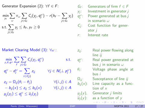
Generator Expansion (2): ∀f ∈ F :
minyf
∑ω
πω∑j∈Gf
Cj(yj , qωj )− r(hf −
∑j∈Gf
yj)
s.t.∑j∈Gf
yj ≤ hf , yf ≥ 0
Gf : Generators of firm f ∈ Fyj : Investment in generator jqωj : Power generated at bus j
in scenario ωCj : Cost function for gener-
ator jr : Interest rate
Market Clearing Model (3): ∀ω :
minz,θ,qω
∑f
∑j∈Gf
Cj(yj , qωj ) s.t.
qωj − dωj =∑i∈I (j)
zij ∀j ∈ N(⊥ pωj )
zij = Ωij(θi − θj) ∀(i , j) ∈ A
− bij(x) ≤ zij ≤ bij(x) ∀(i , j) ∈ A
uj(yj) ≤ qωj ≤ uj(yj)
zij : Real power flowing alongline ij
qωj : Real power generated atbus j in scenario ω
θi : Voltage phase angle atbus i
Ωij : Susceptance of line ijbij(x): Line capacity as a func-
tion of xuj(y), Generator j limitsuj(y): as a function of y
Ferris (Univ. Wisconsin) EMP MOPTA 2011 17 / 27
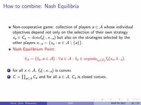
How to combine: Nash Equilibria
Non-cooperative game: collection of players a ∈ A whose individualobjectives depend not only on the selection of their own strategyxa ∈ Ca = domfa(·, x−a) but also on the strategies selected by theother players x−a = xa : o ∈ A \ a.Nash Equilibrium Point:
xA = (xa, a ∈ A) : ∀a ∈ A : xa ∈ argminxa∈Cafa(xa, x−a).
1 for all x ∈ A, fa(·, x−a) is convex
2 C =∏
a∈A Ca and for all a ∈ A, Ca is closed convex.
Ferris (Univ. Wisconsin) EMP MOPTA 2011 18 / 27
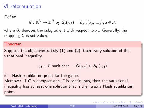
VI reformulation
DefineG : RN 7→ RN by Ga(xA) = ∂afa(xa, x−a), a ∈ A
where ∂a denotes the subgradient with respect to xa. Generally, themapping G is set-valued.
Theorem
Suppose the objectives satisfy (1) and (2), then every solution of thevariational inequality
xA ∈ C such that − G (xA) ∈ NC (xA)
is a Nash equilibrium point for the game.Moreover, if C is compact and G is continuous, then the variationalinequality has at least one solution that is then also a Nash equilibriumpoint.
Ferris (Univ. Wisconsin) EMP MOPTA 2011 19 / 27
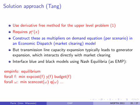
Solution approach (Tang)
Use derivative free method for the upper level problem (1)
Requires pωi (x)
Construct these as multipliers on demand equation (per scenario) inan Economic Dispatch (market clearing) model
But transmission line capacity expansion typically leads to generatorexpansion, which interacts directly with market clearing
Interface blue and black models using Nash Equilibria (as EMP):
empinfo: equilibriumforall f: min expcost(f) y(f) budget(f)forall ω: min scencost(ω) q(ω) ...
Ferris (Univ. Wisconsin) EMP MOPTA 2011 20 / 27
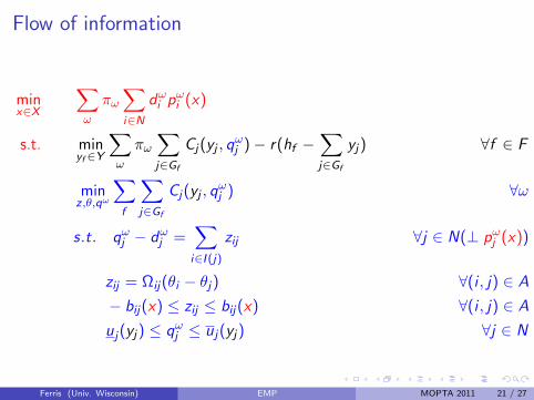
Flow of information
minx∈X
∑ω
πω∑i∈N
dωi pωi (x)
s.t. minyf ∈Y
∑ω
πω∑j∈Gf
Cj(yj , qωj )− r(hf −
∑j∈Gf
yj) ∀f ∈ F
minz,θ,qω
∑f
∑j∈Gf
Cj(yj , qωj ) ∀ω
s.t. qωj − dωj =∑i∈I (j)
zij ∀j ∈ N(⊥ pωj (x))
zij = Ωij(θi − θj) ∀(i , j) ∈ A
− bij(x) ≤ zij ≤ bij(x) ∀(i , j) ∈ A
uj(yj) ≤ qωj ≤ uj(yj) ∀j ∈ N
Ferris (Univ. Wisconsin) EMP MOPTA 2011 21 / 27
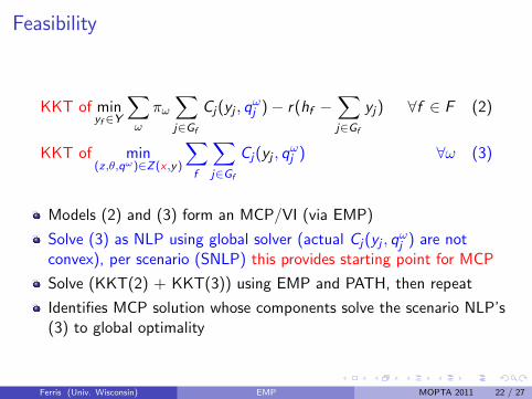
Feasibility
KKT of minyf ∈Y
∑ω
πω∑j∈Gf
Cj(yj , qωj )− r(hf −
∑j∈Gf
yj) ∀f ∈ F (2)
KKT of min(z,θ,qω)∈Z(x ,y)
∑f
∑j∈Gf
Cj(yj , qωj ) ∀ω (3)
Models (2) and (3) form an MCP/VI (via EMP)
Solve (3) as NLP using global solver (actual Cj(yj , qωj ) are not
convex), per scenario (SNLP) this provides starting point for MCP
Solve (KKT(2) + KKT(3)) using EMP and PATH, then repeat
Identifies MCP solution whose components solve the scenario NLP’s(3) to global optimality
Ferris (Univ. Wisconsin) EMP MOPTA 2011 22 / 27

Scenario ω1 ω2
Probability 0.5 0.5Demand Multiplier 8 5.5
SNLP (1):Scenario q1 q2 q3 q6 q8
ω1 3.05 4.25 3.93 4.34 3.39ω2 4.41 4.07 4.55
EMP (1):Scenario q1 q2 q3 q6 q8
ω1 2.86 4.60 4.00 4.12 3.38ω2 4.70 4.09 4.24
Firm y1 y2 y3 y6 y8f1 167.83 565.31 266.86f2 292.11 207.89
Ferris (Univ. Wisconsin) EMP MOPTA 2011 23 / 27
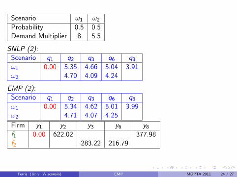
Scenario ω1 ω2
Probability 0.5 0.5Demand Multiplier 8 5.5
SNLP (2):Scenario q1 q2 q3 q6 q8
ω1 0.00 5.35 4.66 5.04 3.91ω2 4.70 4.09 4.24
EMP (2):Scenario q1 q2 q3 q6 q8
ω1 0.00 5.34 4.62 5.01 3.99ω2 4.71 4.07 4.25
Firm y1 y2 y3 y6 y8f1 0.00 622.02 377.98f2 283.22 216.79
Ferris (Univ. Wisconsin) EMP MOPTA 2011 24 / 27
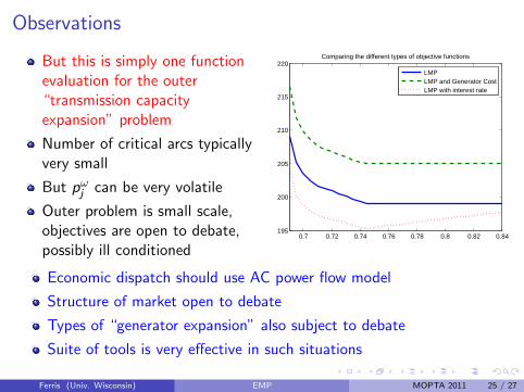
Observations
But this is simply one functionevaluation for the outer“transmission capacityexpansion” problem
Number of critical arcs typicallyvery small
But pωj can be very volatile
Outer problem is small scale,objectives are open to debate,possibly ill conditioned
0.7 0.72 0.74 0.76 0.78 0.8 0.82 0.84195
200
205
210
215
220Comparing the different types of objective functions
LMPLMP and Generator CostLMP with interest rate
Economic dispatch should use AC power flow model
Structure of market open to debate
Types of “generator expansion” also subject to debate
Suite of tools is very effective in such situations
Ferris (Univ. Wisconsin) EMP MOPTA 2011 25 / 27
What is EMP?
Annotates existing equations/variables/models for modeler toprovide/define additional structure
equilibrium
vi (agents can solve min/max/vi)
bilevel (reformulate as MPEC, or as SOCP)
disjunction (or other constraint logic primitives)
randvar
dualvar (use multipliers from one agent as variables for another)
extended nonlinear programs (library of plq functions)
Currently available within GAMS
Ferris (Univ. Wisconsin) EMP MOPTA 2011 26 / 27
Conclusions
Modern optimization within applications requires multiple modelformats, computational tools and sophisticated solvers
EMP model type is clear and extensible, additional structure availableto solver
Extended Mathematical Programming available within the GAMSmodeling system
Able to pass additional (structure) information to solvers
Embedded optimization models automatically reformulated forappropriate solution engine
Exploit structure in solvers
Extend application usage further
Slides available at http://www.cs.wisc.edu/∼ferris/talks
Ferris (Univ. Wisconsin) EMP MOPTA 2011 27 / 27