Mood Management Dynamics:

The Interrelationship between Consumer Mood and Behavior

JAMES D. HESS

JACQUELINE J. KACEN

JUNYONG KIM*

* James D. Hess is Bauer Professor of Marketing Science, University of Houston (email:

jhess@uh.edu). Jacqueline J. Kacen is Visiting Assistant Professor of Marketing, University of

Houston (email: kacen@uh.edu). Junyong Kim is Assistant Professor, University of Central

Florida (emmail: junyong.kim@bus.ucf.edu). Authors’ names appear in alphabetical order and

do not indicate any ranking of contributions to this research. The authors thank the Sheth

Foundation for financial support and participants in the marketing seminar at University of

California-Berkeley for their comments.

Send Correspondence to:

Professor James D. Hess Department of Marketing and Entrepreneurship 375H Melcher Hall College of Business Administration University of Houston Houston, Texas 77204-6283 USA

2

Mood Management Dynamics:

The Interrelationship between Consumer Mood and Behavior

Abstract

People actively attempt to create and maintain positive moods and to escape from

negative moods by engaging in various consumption activities. The principle of homeostasis

explains the essence of this mood-management behavior: that consumers adjust their mood and

activities to preserve constant the conditions of life. We model the dynamics of consumer mood

and mood-management behavior through a pair of interdependent, linear differential equations

and estimate the equations using mood and consumption data collected from an adult consumer

panel. Because empirically fitting continuous-time differential equations to intermittent

observations is uncommon in the marketing literature, we show how to transform differential

equations into equations that can be estimated using simultaneous equation regression methods.

Our consumer panel shows strong homeostasis in mood management and no evidence of

endogenous mood cycles.

Key Words: Mood, Consumer Behavior, Dynamics, Homeostasis

3

Consumers are increasingly turning to the marketplace for products that will help

them to manage their moods and marketers are responding to consumers’ buying behavior

with more and more feel-good products. Hundreds of food, beverage, personal care, and

home products that promote the idea of relaxation, positive mood states, and other forms

of emotional well-being have been introduced into the marketplace in the past few years.

Celestial Seasonings’ “Tension Tamer” tea, Bath & Body Works’ scented candles, bath

salts, and other aromatherapeutic body products, as well as home accessories and feng-

shui kits encourage consumers to actively manage their mood states.

Gardner’s (1985) seminal article on consumer mood states recognized the important role

that mood management plays in a variety of consumer behaviors including service encounters,

selection of retail environments, and shopping. A few marketing studies have sought to

investigate explicitly this process of consumer mood management, that is, to explain the

activities and behaviors undertaken by consumers to maintain a positive mood or repair a

negative mood and the impact of these behaviors on mood (e.g., Kacen 1994; Luomala 1999).

These qualitative studies provide a conceptual understanding of how consumers use consumption

behaviors to manage their moods, but they do not measure the dynamics of this process of mood

management. Mood affects behavior and behavior affects mood in a constantly updating

intertwined system. How, and to what degree, consumer moods motivate particular behaviors

and concomitantly, how engaging in certain behaviors changes a consumer’s mood state are

issues that have not been explored empirically. It is worthwhile to supplement our conceptual

understanding of consumer mood management with an empirical model that measures the

dynamic interrelationship between mood and behavior.

4

In this paper, we address the difficult task of measuring the dynamics of consumers’

mood states and illustrating the corresponding interrelationships between mood and behavior.

We base our study on the key tenet that consumers adjust their mood in accordance with the

principle of homeostasis: that individuals strive to regulate their internal environment to preserve

constant the conditions of life. Given that consumers prefer a relatively constant mood state,

when internal or external events disrupt their natural mood state, consumers engage in behaviors

to help them restore their mood to its normal (i.e., homeostatic) level.

Our methodology for identifying and explaining the process of mood management

integrates panel data collected from an adult consumer sample with a model for data analysis that

incorporates simultaneous differential equations. The model in our study accommodates several

aspects important to demonstrating the dynamics of consumer moods and mood management:

1. The model captures the active nature of the mood-management process. Not only

does our model clarify how mood responds to consumption behaviors, but it also

illuminates how consumption behaviors are chosen with mood improvement in mind.

2. Mood, a transient affective state, adjusts continuously over time. Yet, at best, mood

can only be measured at intermittent times. We show how the continuous mood

adjustment process can be understood from discrete mood observations.

3. Psychological homeostasis interlinks mood and consumption behavior, so we use a

two-stage least-squares estimation procedure to avoid biased parameter estimates.

5

This model is applied to multiple daily measures of mood and behavior data collected

from our consumer panel over a period of five days. We describe how we fit the differential

equations to the model, discuss the empirical findings and their implications for consumer

research, and evaluate the contribution of the model to our understanding of consumer behavior.

Finally, we present limitations and issues for further research.

MOODS AND MOOD MANAGEMENT

Moods and mood management are widely recognized phenomena in both the psychological and marketing literatures. Moods are generalized feeling states that are transient in nature (Gardner

1985). This definition distinguishes moods from emotions, which are object-focused as opposed to generalized, and from attitudes or temperaments, which are enduring states (Clore et al. 2000). A critical element of this definition of mood is that it is transient; therefore, moods are subject to

change over time.

People manage their moods when they experience them and many of the responses are

directly related to consumption and purchases, as the examples at the beginning of the paper

demonstrate. Research has shown that people actively attempt to maintain positive mood states

and to escape from negative moods states by engaging in various consumption activities

including eating, watching television, shopping, socializing with friends, going to a movie,

listening to music or exercising (Eliashberg and Sawhney 1994; Faber and Christenson 1996;

Holbrook and Gardner 2000; Morris and Reilly 1987; Thayer, Newman, and McClain 1994;

Zillmann 1988). The operational conceptualization of mood management is that consumers’

moods prompt mood-managing behaviors, and that engaging in mood-managing behavior

induces changes in mood, which subsequently elicits changes in behavior. Psychological Inquiry

recently dedicated an entire issue to the topic of mood management (2000, Vol. 11, No. 3),

presenting several theories of mood regulation (none offered empirical data concerning the

dynamic interrelationship between mood and behavior).

6

Most mood studies focus only on the effect of moods in one time period, treating mood

as a simple independent or dependent variable within a before-and-after experimental design

(e.g., Barone, Miniard, and Romeo 2000; Batra and Stayman 1990; Lee and Sternthal 1999;

Swinyard 1993). Moods are a dynamic phenomenon. The interaction between mood and

behavior necessarily causes changes over time. Yet this dynamic and evolving nature of mood

and behavior largely has been ignored in previous marketing studies. Two notable exceptions

are Holbrook and Gardner’s (2000) study that examined how people’s mood changed over time

as a result of listening to music, and Eliashberg and Sawhney’s (1994) study that explored the

dynamic effects between initial mood state and the emotional characteristics of scenes from a

movie on participants’ subsequent mood state and overall enjoyment of the movie.

Baumgartner, Sujan, and Padgett (1997) examined students’ moment-to-moment emotional

responses to television ads in a single-variate correlational analysis, but did not measure the

dynamics of participants’ affective reactions.

However, even while the Holbrook and Gardner (2000), Eliashberg and Sawhney (1994),

and Baumgartner et al. (1997) studies focused on the effects of the consumption experience on

mood changes over time, the affective stimuli and the consumption experiences were exogenous

variables determined by the experimental research design. How do mood dynamics play out in a

naturally occurring setting? How does mood change when consumers are allowed to freely

choose the consumption experience? How do different types of consumption experiences affect

changes in consumers’ moods?

The objective of the present study was to investigate the dynamic nature of mood in a

naturally occurring context, and to explain how consumers adjust their mood-managing

behaviors in response to the moods they experience in their daily lives. Because many of these

7

mood-managing behaviors are related to consumption activities, the present study provides

insights into understanding the choices consumers make and the affective characteristics of select

consumption activities. Drawing upon the experiential view suggested by Holbrook and

Hirschman (1982), the mood maintenance/mood repair hypothesis described by Isen (1984), the

two-dimensional measure of mood promulgated by Russell, Weiss, and Mendelsohn (1989), and

the concept of psychological homeostasis promoted by Schulze (1995), we propose a model for

measuring the dynamic process of mood management.

MODELING THE DYNAMIC PROCESS OF MOOD MANAGEMENT

Homeostasis

Homeostasis is the process by which individuals seek to regulate their internal

environment. This construct’s origin is in physiology and biochemistry (see Canon 1932): when

an organism is cold (the state) it shivers (the behavior) to generate heat and thus move toward the

normal temperature. The theory behind homeostasis is that an organism can survive only if the

physiological system linking the state to the behavior is internally stable.

Psychologists expanded the concept of homeostasis to include psychophysiological states

(such as moods and feelings) recognizing the interrelationship between biological factors and

psychological factors (see Berntson and Cacioppo 2000; Weisfeld 1982). According to this

approach, human survival depends in part on the stability of the psychological system linking

moods and behavior. This process creates physical and psychological needs that influence mood

and affect-related behaviors (Edlund 1987; Parker and Tavassoli 2000). Studies of psychological

homeostasis (Headey and Wearing 1989) support the theoretical foundation of our model,

8

especially Headey and Wearing’s (1989) dynamic equilibrium model of well-being in which

individuals are assumed to have “normal” equilibrium levels of subjective well-being (SWB).

Their study investigated the dynamic relationship between personality, life events, and SWB

using data from an Australian panel.

Applying the concept of psychological homeostasis to the process of mood management

suggests the following description of the dynamics by which moods are managed. People want

to remain in a comfortable affective state. In order to achieve stability, their unconscious and

conscious psychological systems have built-in error-correction capabilities. The homeostatic

dynamic system proposed here assumes that the farther away an individual is from the most

comfortable levels of mood and behavior, the more rapidly s/he returns toward these normal

mood and behavior states. The normal level of mood (or behavior) is a state that leaves the

person most comfortable and satisfied.1 This implies that as a consumer approaches normal

states of mood and behavior, the speed of closure (i.e., rate of change of mood or behavior)

naturally diminishes to prevent overshooting.

Specifically, suppose that the measurement of mood has been scaled so that the normal

mood level is . If the mood state is M(t) at time t, then the time rate of change of mood is in

direct proportion to the discrepancy between current mood and normal mood, - M(t). If the

current mood falls short of normal, then this difference is positive and the time rate of change of

M̂

M̂

1 The normal mood state should not be thought of as some hypothetical zero point on a dimensional map of mood. Findings from psychological research indicate that some individuals have higher natural arousal states (Diener et al. 1985; Kohn 1987; Steenkamp, Baumgartner, and van der Wulp 1996) or higher levels of negative affectivity (Larsen and Ketelaar 1991; Watson and Clark 1984). Isen (1984) argues that, in general, we prefer to be in slightly positive mood states (cf. Zuckerman’s [1994] research into sensation-seeking which characterizes the ideal level of stimulation as the amount of stimulation a person prefers in general. Similarly, Steenkamp and colleagues [Steenkamp et al. 1996; Steenkamp and Baumgartner 1992] found that psychological pleasantness is highest at the level of stimulation at which a person feels most comfortable, what they refer to as the Optimal Stimulation Level. Their Need for Stimulation scale measures a person’s distance from the OSL. Individuals may have different normal mood states and therefore, different homeostatic mood levels.

9

mood is positive: mood levels rise. The greater the degree to which the current mood level falls

below normal, the greater is the feeling of deficiency, and the more rapidly the system self-

corrects the situation. Conversely, if current mood is only slightly below normal, the consumer

feels less urgency and the psychological homeostasis system moves more slowly. This system

reverses itself if the current mood exceeds the normal mood level.

The principle of homeostasis suggests more than the existence of equilibrium levels of

physiological and psychological variables. It implies that individuals have powerfully stable

self-correcting systems. If the time rate of correction of mood were a constant, then the

momentum of mood improvement would certainly carry the consumer past the normal mood

level. If the psychological system has evolved to make people affectively stable in the normal

course of their lives, it makes sense that the speed adjusts as the mood level approaches normal.

The proposed dynamic homeostasis system can be represented as a differential equation.

In the simplest version of our homeostatic dynamic model, )t(M))t(M0(dt

)t(dMα−=−α= , the

normal mood level is zero for simplicity of exposition, and α is a positive parameter that

measures the innate rate of mood correction. The negative sign in this equation indicates that the

mood system is self-correcting: when the mood state is positive, mood will be reduced; when it

is negative, it will be increased. The more intense the current mood is, the faster its adjustment.

This differential equation may be rearranged algebraically to read α−=M

dt/dM . On the

left hand side of this formula is the percentage rate of change of mood. Homeostasis dynamics

indicates that the percentage rate of change of mood is a constant. When the mood is less

intense, then the absolute speed of mood correction is slower in order to maintain a constant

percentage rate of change, as previously noted.

10

Mood Dynamics

The above description provides our basic translation of homeostasis into a dynamical

mood system. The simple model can be modified to incorporate mood management. Let B(t) be

the current level of behavior that influences the person’s mood state. Details of such behaviors

will be provided below, but they can be thought of as either endogenous mood-managing

behaviors (e.g., going shopping, buying an ice cream cone) or exogenous activities that influence

the person but are not guided by the mood state (e.g., hearing a favorite song on the radio). Such

behaviors occur in the normal course of everyday life, so B denotes the baseline level at which

this behavior, or set of behaviors, is performed. For example, might represent the typical

quantity of ice cream or sweets consumed per period.

ˆ

B̂

Active mood management is captured in our model by including behavior in our

differential equation for mood:

]B̂B(t)[]M(t)M̂[dt

dM(t)−β+−α= , (1)

where α and β are parametric constants. The first term on the right hand side follows directly

from the previous discussion of mood homeostasis: is the normal mood level and α is the

innate rate of mood correction. The second term indicates that when behavior exceeds the

baseline level, it contributes to a more rapid adjustment upward in mood state: is the baseline

behavior level and β is the responsiveness of mood to behavior. If behavior is at its baseline

level, B(t)= , then the mood adjustment follows the basic homeostatic mood dynamics alone.

However, if behavior is more intense than typical in the sense that B(t) - is positive and the

parameter β is positive (e.g., larger quantities of ice cream are consumed), then the behavior

M̂

B̂

B̂

B̂

11

contributes to an increase in mood velocity (e.g., more rapid mood improvement).2 On the other

hand, if behavior falls below the baseline level, mood velocity is diminished. So people in

negative moods can repair them by engaging in positive behaviors, while people in positive

moods can prolong their mood by increasing positive behaviors. The inhibiting rather than

stimulating nature of some behaviors also would be reflected in a negative value for the

parameter β.

Mood-Managing Behavior Dynamics

The mood dynamics equation (1) explains the dynamics of internal mood state changes as

the consequence of both the natural homeostasis of moods and the reaction of moods to overt

behaviors and activities. But the equation does not provide an explanation of how behavior may

change over time. Because prior studies indicate that people actively manipulate their behavior

to influence their moods, we model the dynamics of mood behavior using the following

differential equation to explain the rate of change of behavior:

[ ] [ ])t(BB̂M(t) -M̂ dt

)t(dB−δ+γ= . (2)

The first term on the right hand side of (2) describes the way that mood influences

adjustments in behavior. The parameter γ is a measure of the combination of a consumer’s

motivation and capability to manage mood. It could be large because the consumer has a strong

desire to control mood by his or her actions. Alternatively, γ could be small if the consumer has

time or other resource constraints that make behavioral adjustments to mood difficult.

2 Velocity has speed and direction. If the mood level is increasing, then more-intense-than-baseline behavior causes the mood to change at an even faster rate. Less obviously, if the mood level is declining, then more-intense-than-baseline behavior causes the mood to decline at a slower rate, or even to change directions to an upward trajectory. If the mood level is increasing, then less-intense-than-baseline behavior causes the mood to rise at a slower rate, and if the mood level is declining, then less-intense-than-baseline behavior causes it to fall at an even faster rate.

12

The parameter M̂ denotes the normal level of mood for the individual, as discussed

above (see footnote 1). Implicit in the term “normal” is the idea that affective states can be either

too low or too high. Arousal and pleasure may reach such high levels as to create mood states of

excruciating agitation or euphoria in the over-stimulated individual, and they may reach such low

levels as to produce mood states of dreary sadness. The parameter M̂ quantifies the level of

mood that would leave the individual most comfortably satisfied in the end (see footnote 1).

If the mood is below the normal level, the velocity of behavior increases, but if it is above

the normal level, then velocity of behavior diminishes. As in footnote 2, if the behavior level is

diminishing, an increase in velocity means that the rate of decline drops or even switches from a

declining to an increasing trajectory.

The second term on the right hand side of equation (2) describes the way that current

behavior level influences adjustment in behavior. Just as the internal psychology of moods is

driven by homeostasis, we assume that homeostasis also applies to behavior. In particular, if the

current level of behavior falls short of the baseline behavior, , then the person attempts to

correct this situation. The more current behavior differs from the baseline, as measured by B(t) -

, the faster is the speed of adjustment; conversely, the more the current behavior approximates

the baseline behavior, the slower is the speed (again, this is suggested by homeostasis).

B̂

B̂

The behaviors individuals employ to manage their moods are not cost-free. Shopping

requires time and money; eating too much ice cream may entail psychological cost in the form of

guilt or regret. Such costs are captured by a positive parameter δ in equation (2), which denotes

an innate rate of behavior correction. The more costly deviations from normal behaviors are to

individuals, the more intensely they correct them.

13

In conclusion, differential equations (1) and (2) model the dynamic interdependence of

mood and the behaviors employed to manage the mood. The interdependency of mood and

behavior can lead to interesting patterns, including endogenous mood cycles, as demonstrated in

the next section.

DYNAMIC PATTERNS OF MOOD MANAGEMENT

In analyzing the dynamics of mood and behavior that result from equations (1) and (2),

there are two distinct issues to be considered: what is equilibrium and what is the path toward

equilibrium? Equilibrium consists of values of mood and behavior adjusted to one another so

there is no inherent tendency for either to change. The equilibrium mood level, the level toward

which homeostasis drives mood, is the individual’s normal mood level, (recall that this

normal mood level may be different for each individual). The equilibrium behavior level is the

baseline behavior for each individual, . At these baseline levels, equations (1) and (2) indicate

that the time rate of changes are zero.

M̂

B̂

Time Paths of Mood and Behavior

The equilibrium levels of mood and behavior have been described above. We

now describe the time path out of equilibrium implied by equations (1) and (2). Given

that linear differential equations have solutions that are of an exponential form,

and , the value of the parameters in these functions are identified

by studying the homogenous version of the system of differential equations:

atme)t(M = atbe)t(B =

.)t(B)t(M

dt)t(dB

dt)t(dM

⎥⎦

⎤⎢⎣

⎡⎥⎦

⎤⎢⎣

⎡δ−γ−

βα−=

⎥⎥⎥

⎦

⎤

⎢⎢⎢

⎣

⎡

(3)

14

The derivatives of the above exponential functions are .

Substituting into the matrix equation (3) and canceling the common term e

atat bae)t('B,mae)t('M ==

at results in:

⎥⎦

⎤⎢⎣

⎡=⎥

⎦

⎤⎢⎣

⎡⎟⎟⎠

⎞⎜⎜⎝

⎛⎥⎦

⎤⎢⎣

⎡−⎥

⎦

⎤⎢⎣

⎡δ−γ−

βα−

⎥⎦

⎤⎢⎣

⎡=⎥

⎦

⎤⎢⎣

⎡⎥⎦

⎤⎢⎣

⎡δ−γ−

βα−

00

bm

1001

a

orbm

abm

(4)

The values of a and [m b]’ that satisfy these equations are the characteristic values and

characteristic vectors of the dynamics matrix C ≡ (sometimes called the eigenvalues

and eigenvectors of C).

⎥⎦

⎤⎢⎣

⎡δ−γ−

βα−

3 In particular, the coefficient a in the exponential solution eat is a

characteristic value of C, and it can take on two values:

24)(

a,a2

21βγ−δ−α±δ+α

−= . (5)

In the normal course of events, both characteristic values a1 and a2 are negative real

numbers (they are real numbers when (α-δ)2-4βγ>0). Specifically, if a1⋅a2=αδ+βγ>0, then the

two characteristic values have the same sign; if, in addition, a1+a2= -(α+δ)<0, then the

coefficients’ common sign is negative. Negative exponential functions asymptotically approach

zero; if this is the case, it would indicate that both mood and behavior move steadily toward their

equilibrium values as predicted by homeostasis.4

Mood Cycles

The radical in formula (5) suggests the other possibility: that the interplay between

behavioral adjustments and internal mood states can create mood cycles. Specifically, if the term

3 The dynamics matrix C has built-in sign patterns; e.g., the diagonal elements are negative.

15

under the radical, (α-δ)2-4βγ, is negative then the characteristic values are complex numbers with

a real part (α+δ)/2 and an imaginary part 4/)(i 2δ−α−βγ± , where 1i −≡ . This does not

imply that moods or behavior are “imaginary,” but rather that mood dynamics involve cycles.

This is because exponential functions and sinusoidal functions are linked through imaginary

numbers by the fundamental identity: e-it = cos(t) - i sin(t). When (α-δ)2-4βγ<0, then mood

management will involve sinusoidal paths oscillating above and below the equilibrium mood

levels (see Figure 1).

_______________________ Insert figure 1 about here

⎯⎯⎯⎯⎯⎯⎯⎯⎯⎯⎯⎯⎯⎯⎯⎯⎯

Cyclical moods occur when the term (α-δ)2 is small in comparison to the term βγ. Recall

that the values of α and δ measure the innate strength of the homeostatic system for mood and

behavior, respectively. Even if moods return rapidly to normal levels (α is large), if the cost of

making behavioral adjustments is similarly large (δ≈α), then mood is stable but difficult to

control. Recalling that the values of β and γ measure the responsiveness of mood to behavior

and the motivation/capability to manage behavior, respectively, if these parameters are positive

and large, then consumers will be active mood managers. Vigorously manipulating a difficult-

to-control mood management system results in “oversteer” that creates endogenous mood cycles.

These cycles are not necessarily pathological, but could represent the problems of coordinating

the cognitive, affective, and behavioral changes of normal, healthy life.

4 The solution is a weighted combination of two negative exponential functions. If one weight is positive and the other negative, the solution can overshoot the equilibrium once before converging exponentially from the other side.

16

DATA

Consumer Mood Panel

To discover the actual dynamic patterns of mood-management behavior through an

empirical test of our model, 93 consumers over the age of 21 were recruited to participate in a

“Consumer Mood Panel Survey” in which mood and behavior data were collected by telephone

three times a day over a five-day period. After agreeing to participate in the study, panelists

received a wallet-sized Mood Grid card (see below) and a general explanation of the study.

Prior to the start of the panel interviews, panelists were asked about their likely

participation in a number of activities and behaviors, responded to demographic questions, and

were given instructions on use of the Mood Grid. The average panelist was 39 years old,

college-educated, and working in a professional or managerial occupation. Seventy percent were

female. See Table 1 for a detailed description of the panelists. _______________________

Insert Table 1 about here ⎯⎯⎯⎯⎯⎯⎯⎯⎯⎯⎯⎯⎯⎯⎯⎯⎯

Mood and behavior data collection for all participants began on Monday morning and

ended on Friday evening. The recurring panel interviews were scheduled at the convenience of

the panelist but always included a morning, an afternoon, and an evening contact. In total, 1,395

interviews were completed, each lasting approximately five minutes. These short phone

interviews measured consumers’ current mood and their participation in any of a variety of

activities since the last contact, as described in the next section.

Measuring Mood and Behavior

The underlying dimensional structure of mood is not a settled question, but most

researchers agree that moods can be described in terms of their degree of arousal, whether one

feels excited or relaxed, and their valence, whether they are pleasant or unpleasant (e.g., Cohen

17

and Areni 1991; Holbrook and Gardner 2000; Mano and Oliver 1993; Parkinson et al. 1996). As

Holbrook and Gardner (2000, p. 167) state, “Although the structure of moods, emotions, and

other affective states is somewhat controversial, several studies have found consistent evidence

for the existence of two primary dimensions – pleasure and arousal (Russell 1980).”

For this study, we used Russell et al.’s (1989) Affect Grid to measure mood. It consists

of a nine-by-nine grid labeled (1) “high arousal” to (9) “sleepiness” on the vertical dimension

and (A) “unpleasant feelings” to (I) “pleasant feelings” on the horizontal dimension. During

each phone interview, panelists indicated their current mood by providing the row and column

coordinates (e.g., “D, 4”) on the wallet-sized Mood Grid card that responded to their feelings at

the moment. From this, two mood measures were constructed on a 9-point scale: a pleasure

component, where 9 indicates high pleasure, and an arousal component, where 9 indicates high

arousal.

The Russell et al. (1989) Affect Grid was chosen for its ease of use in this panel study,

where repeated measures of consumers’ mood and behavior were gathered via a phone interview.

Unlike time-consuming multiple-item questionnaires or checklists, the Affect Grid is ideal for

repeated observations (Russell et al. 1989, p. 493). Russell and his colleagues found that scores

from the Affect Grid were highly correlated with scores obtained using longer, more time-

consuming verbal self-report scales. The Affect Grid has been used in other marketing studies as

a reliable measure of consumer mood states (see Dubé, Chebat, and Morin 1995; Holbrook and

Gardner 2000).

A variety of activities are available to help consumers manage their moods including

eating something, watching television, shopping, calling a friend, listening to music, or going for

a run. Consumers may aggregate activities based on their “affective benefits” or similarity of

18

impact on mood. For example, watching television or listening to music may have comparable

influences on arousal, and act as substitutes for each other on other non-mood related wants.

Previous researchers (Morris and Reilly1987; Thayer et al. 1994; and Zillmann 1988) have

suggested particular groupings of behaviors based on consumer self-report or factor analyses of

behavioral data. However, the identified groupings are neither mutually exclusive nor consistent

across studies. Rather than relying exclusively on prior research, we conducted a preliminary

survey of 220 students, asking them to evaluate how a variety of activities make them feel on a

9-point scale of unhappy-happy (pleasure) and relaxed-excited (aroused). Our research focused

on five aggregate activities (shop, socialize, watch TV, listen to music, and eat out).

Figure 2 displays respondents’ beliefs concerning how these activities influence their

mood dimensions of arousal and pleasure. The activities Shop and Socialize are more pleasing

than the average pleasure provided by each of the other items in the survey but they are not

significantly different than the average arousal of all other items.5 The activities Music and TV

are significantly less arousing (that is, more calming) than the other behaviors but not more

pleasing. As a result of our student survey results, we created two behavior category variables

from the activities measured in our consumer panel survey: Amusement and Relaxation.

Amusement consists of shopping or socializing with others. Relaxation consists of watching

television or listening to music.

_______________________ Insert figure 2 about here

⎯⎯⎯⎯⎯⎯⎯⎯⎯⎯⎯⎯⎯⎯⎯⎯⎯

5 The differences discussed here are all significant at the 1% level.

19

In our consumer panel survey each of these common behaviors were measured with a

three-item scale. The number of behaviors was limited to keep the questionnaire short to prevent

panelist fatigue and dropout. The first scale item for each behavior measured the length of time

(in minutes) that panelists participated in the activity. The other two scale items measured the

intensity with which panelists engaged in the activity. See Table 2 for a list of the behavior item

measures used in the consumer panel study. We do not try to explain a consumer’s selection

between TV or music activities, but rather try to understand the total amount of relaxing

activities selected. Our independent data indicates that Eating Out is both more pleasing and less

arousing than other behaviors, so the Dining behavior of panelists is used as a covariate in the

empirical mood model.

_______________________ Insert Table 2 about here

⎯⎯⎯⎯⎯⎯⎯⎯⎯⎯⎯⎯⎯⎯⎯⎯⎯

It is important to note that in each interview we measured the current mood state of the

panelist, and the behaviors the panelist engaged in since the last interview. As a result, mood

and behavior data are not contemporaneous. To illustrate, in the dinnertime interview panelists

reported their current evening mood but they reported behaviors that occurred in the early

afternoon. We account for this asynchronism in the empirical estimation of the mood

management dynamics, described in the next section.

Predicted Relationships Between Measured Variables and Derivatives

Homeostasis implies that both moods and behaviors are self-correcting. In terms of the

general parameters of the simple two-variable model presented in equations (1) and (2), this

corresponds to the hypotheses -α<0 and -δ<0. Applying these theoretical restrictions to the

20

specific measures of mood (Pleasure and Arousal) and mood-management behaviors

(Amusement and Relaxation) constructed from our data set, all the elements on the diagonal

equation (3) are hypothesized to be negative.

Our preliminary student survey indicated that Amusement activities (shopping or

socializing) have an influence only on Pleasure (see Figure 2), while Relaxation activities

(watching television or listening to music) have an influence only on Arousal (see also

Csikszentmihalyi and Kubey 1981; Thayer et al. 1994; Zillmann 1988)6. Dining influences both

mood dimensions according to our data, but while one’s mood may influence what is ordered

and consumed, the activity of dining probably is driven more by non-mood factors (time of day,

business, family activities), so we treat it as an independent covariate.

Homeostasis, which implies that the entire mood-management system is stable, requires

assumptions about the non-diagonal parameters as well as the diagonal ones. For the simple

two-variable model, stability requires that αδ+βγ>0; in other words, the diagonal elements of the

dynamics matrix C ≡ dominate the off-diagonal elements (in magnitude).⎥⎦

⎤⎢⎣

⎡δ−γ−

βα− 7 The

stability of the entire mood-management system is investigated through a Monte Carlo

simulation of the characteristic values using the estimated statistics of C.

Whether or not the parameters of responsiveness of mood to behavior (β) or the

motivation/capability to manage behavior to correct mood (γ) are positive or negative depends on

the particular measures of mood and behavior. We first discuss mood adjustments to behavior.

6 It should be noted that although in some circumstances pleasure and arousal have common causes and hence are correlated, they do not have a direct causal link and have been found to be independent dimensions of mood (Diener and Emmons 1984; Green and Salovey 1999; Russell et al. 1989, Russell and Pratt 1980). As a result, Pleasure and Arousal are treated as independent constructs in our model and are not linked through the differential equations. 7 The necessary and sufficient Routh-Hurwitz conditions for stability are more complicated to formulate for more than two variables (Samuelson 1947).

21

The rate of change of Pleasure should increase if Amusement behaviors (shop or socialize) occur

since these specific activities are inherently enjoyable (βamusement>0). The Relaxation behaviors

(watch TV, listen to music) are sedentary behaviors that are likely to decrease changes in arousal

rates (βrelaxation<0; see Bryant and Zillmann 1984; Csikszentmihalyi and Kubey 1981; Thayer et

al. 1994; Zillmann 1988).8

A similar pattern is manifest in the model’s predictions concerning behavioral

adjustments to mood levels. If a person is feeling less pleased than is normal, s/he is motivated

to increase the rate of Amusement behaviors (γpleasure>0). The rate of change of Amusement is

influenced positively by γpleasure( -P(t)), but that means that it is negatively impacted by

increases in the current level of Pleasure. This can be confusing at first blush. If a person’s

Arousal level is at a less than normal level, homeostasis requires that s/he decrease the rate of

increase in Relaxation behaviors (γ

P̂

arousal<0). This implies that the sign of the response of

Relaxation behavior to increases in Arousal is positive.

FITTING CONTINOUS DIFFERENTIAL EQUATIONS TO INTERMITTENT DATA

The dynamic mood-management process is assumed to adjust continuously in time

although our measures of mood and behavior reflect data collected at intermittent times. The

empirical estimation of such continuous-time models, while common in economics (Bergstrom

1976; Gandolfo 1993; Phillips 1974), is less common in the marketing literature (one exception

8 Of course, watching television or listening to music can be either stimulating or relaxing depending on the genre of the material. An action-adventure show produces a different affective response than a nature documentary (Zillmann 1988). We accounted for this in our three-item activity measures by measuring the type of entertainment chosen, and coding the Relaxing behaviors so that higher values represent more engaging, relaxing fare. Music tempo was reverse coded for this reason.

22

is Dubé and Morgan 1998). For clarity of exposition, we present a simple version of our mood

differential equation:

)t(u)t(B)t(Mdt

)t(dM+β+α−= . (6)

The normal levels of mood and behavior do not appear in equation (6), but the error term, u(t), is

assumed to be an independent random variable with mean zero, variance σu2 and zero

autocorrelation (that is, E[u(s)u(t)]=0, s≠t). Suppose that mood is observed at equally spaced

times t1,..,tN, with one time unit between observations. For times between observations the

dynamic mood-behavior process continues unabated but unmeasured.

Integrating the differential equation from time ti-1 to ti:

( )

∫∫∫

∫∫

−−−

−−

+β+α−=−

+β+α−=

−i

1i

i

1i

i

1i

i

1i

i

1i

t

t

t

t

t

t1ii

t

t

t

t

.dt)t(udt)t(Bdt)t(M)t(M)t(M

or,dt)t(u)t(B)t(Mdtdt

)t(dM

(7)

The integral of the derivative of mood on the left-hand side equals the change in mood from ti-1

to ti by the Fundamental Theorem of Calculus.

To explain the change in mood in this time interval, we compute the cumulative recent

history of mood and cumulative behavior from time t∫−

i

1i

tt dt)t(M ∫

−

i

1i

tt dt)t(B i-1 to ti. Although the

values of M(t) and B(t) are not known in the interval between ti-1 and ti, the cumulative mood can

be approximated by the trapezoid seen in Figure 3, which requires only knowledge of mood at

the ends of the interval. The trapezoid rule implies that .2/))t(M)t(M(dt)t(M 1ii

t

t

i

1i

−+≅∫−

_______________________ Insert figure 3 about here

⎯⎯⎯⎯⎯⎯⎯⎯⎯⎯⎯⎯⎯⎯⎯⎯⎯

23

As noted in the description of the panel data, measured behavior chronologically predates

measured mood: when we interviewed the panelists at time ti we asked about their mood at that

time, but asked about behavior that had occurred between the prior interview at time ti-1 and the

current interview at ti. In other words, the measured behavior occurred neither at ti nor at ti-1, but

rather in the interval [ti-1,ti]. In our model estimation, we assume that the measured behavior

corresponds to the midpoint, ½ti-1 + ½ti and consider this asynchronicity, as follows.

The cumulative behavior is represented by the shaded area ti-1VKUti in Figure 4. The

behavior measured during the interview at time ti occurred earlier, at point K. The above

trapezoid rule produces the trapezoid CIKD, but the area represented by CIKD is a poor

approximation of the desired cumulative behavior measure. A better approximation is the sum

of the two trapezoids ti-1JKD and DKLti (the second is a rectangular trapezoid). This double

trapezoid approximation of cumulative behavior is )t(B)t(Bdt)t(B i87

1i81t

ti

1i+≅ −∫

−.

_______________________

Insert figure 4 about here ⎯⎯⎯⎯⎯⎯⎯⎯⎯⎯⎯⎯⎯⎯⎯⎯⎯

Using these trapezoidal approximations of cumulative mood and behavior measures, the

discrete version of the continuous differential equation (6) is

( ) ( ) ii87

1i81

1i21

i21

1ii BBMMMM ε++β++α−=− −−− , (8)

where Mi denotes the observed value M(ti), and so forth. Because in equation (6) u(t)’s mean is

zero, the mean of the cumulative error in equation (8), εi ≡ is also zero. The variance

of ε

∫−

i

1i

tt dt)t(u

i equals σu2 and zero autocorrelation implies cumulative errors are uncorrelated. By similar

reasoning, the equation that explains the change in behavior at time ti is

( ) ( ) i1i21

i21

2i81

1i87

1ii BBMMBB θ++δ++γ−=− −−−− . (9)

24

The mood equation (8) and the behavior equation (9) form the proper basis for the empirical

estimation of the continuous-time differential equations (1) and (2).

A much simpler, but less faithful, translation of the continuous-time mood dynamics

model into a discrete time model involves replacing the derivative by the difference and

replacing mood and behavior by lagged discrete values:

ii1i1ii BMMM ε+β+α−=− −− , (10)

i1i1i1ii BMBB θ+δ+γ−=− −−− . (11)

(Note that the lagged value of behavior was measured at time ti in our panel.) For example, Kim,

Bridges, and Srivasta (1999) employed this discrete-time estimation method in their model of

sales diffusion. In this discrete version, cumulative mood and behavior are tacitly measured by

rectangular rather than trapezoidal approximations. This implicitly assumes that mood and

behavior are not changing in the time interval [ti-1, ti]. For exponential functions (the basic

solution for the equations), the rectangular approximation is less accurate than the trapezoidal

approximations in proportion to the exponential coefficient and the square of the time between

observations. For our intermittent observations of rapidly adjusting moods, the trapezoidal

approximations are superior to rectangular approximations (Bergstrom 1993).

ESTIMATION OF MOOD MANAGEMENT DYNAMICS

Two Stage Least Squares

Simultaneous equation regression methods are required to estimate mood and behavior

equations like (8) and (9) because the unobserved error term in each equation is likely correlated

with one of the explanatory variables in that equation, and as a result, ordinary least squares

estimates are biased. Although a wide variety of simultaneous equation methods exist, we use

25

two-stage least-squares rather than a joint equation technique such as three-stage least-squares,

full-information maximum likelihood, or LISREL because in these joint techniques, any

specification error in one equation contaminates the estimates of all equations. In our model, a

multitude of factors determines consumption activities like shopping, watching television, or

listening to music. Recognizing that our panelists did not provide details on the idiosyncratic

factors that may have influenced their behavior, we are cautious about the capability of our data

to explain these behaviors. To prevent contaminating the estimates of the mood equations by

errors from the behavior equations, we use the single-equation method two-stage least-squares.

Pooling Data and Moderator Variables

The Consumer Mood Panel Survey provides cross-sectional and time-series data. In

order to estimate the parameters of the mood-management system, we pooled the data for all 93

panelists into a grand time series for our primary analysis. That is, we assume that α, β, γ, δ are

identical for all consumers.9

Since it is easier for consumers to adjust their behaviors when there are fewer demands

on their time resources, consumers’ motivation and capability to manage their mood with

behavior, γ, may vary with the time of day. This heterogeneity is captured by a time-of-day

variable in the moderator formula: γi=γ0+γ1Time-of-Dayi. Time of day (ToD) takes on three

values corresponding to morning, afternoon, and night. We dummy code two of these day-parts

9 Admittedly, the rate at which mood corrects itself, the responsiveness of mood to behavior, consumers’ motivation and capability to manage their moods, and the rate of behavior correction could be different for different consumers. Our model of the dynamics of mood management captures the overall process of the entire panel sample. Panelist-specific estimation of (12) and (13) is not viable because only fourteen useable observations are provided by each panelist and fourteen parameters must be estimated (seven coefficients and their standard errors). However, we present the results of a segmentation analysis of sex differences in mood management in the Discussion section at the end of the paper and we welcome future studies that explore differences among consumer segments.

26

to estimate the different values of γ in each remaining day-part. Substituting this moderator

formula into equations (8) and (9) gives the estimation equations

( ) ( ) ii87

1i81

1i21

i21

01ii BBMMmMM ε+++β++α−=− −−− , (12)

( ) ( ) ( ) i1i21

i21

2i81

1i87

i1

2i81

1i870

01ii BBMMToDMMbBB θ++δ++γ−+γ−=− −−−−−− . (13)

The interaction term, ( )2i81

1i87

i MMToD −− +⋅ , allows us to estimate the change in behavior

dynamics during different parts of the day.

27

EMPIRICAL RESULTS

As previously discussed, we measured the mood of our panelists along the two traditional

dimensions, pleasure and arousal. We estimated a separate equation for the rate of change in

mood for each dimension, using as explanatory variables the trapezoidal approximation of

cumulative mood (e.g., Pleasure) and the double trapezoidal approximation of the corresponding

cumulative behavior (e.g., Amusement). The measured behavior actually occurred prior to the

mood measure, so the cumulative behaviors are exogenous. The cumulative mood is

endogenous, justifying the use of two-stage least-squares.10

Two separate behavior equations were estimated to explain the rate of change in

Amusement and Relaxation behaviors, using as explanatory variables the trapezoidal

approximation of cumulative behavior, the double trapezoidal approximation of the

corresponding cumulative mood dimension, and the product of day-part dummy variables with

cumulative mood (the moderator variable for time of day). The three dummy variables,

Morning, Afternoon, and Evening, were rotated through the model specification for behavior

dynamics to obtain the relevant t-statistics without the need for more cumbersome (but

equivalent) calculations involving the covariances of estimated moderator coefficients (see

Kacen and Lee 2002).11

Table 3a summarizes the Pleasure management system with Amusement behavior and

Table 3b summarizes the Arousal management system with Relaxation behavior. Our spartan

10 The instruments in our two-stage least-squares regression equations consisted of gender, household size, moods and behaviors lagged one period and interacted with gender, dining and dining interacted with gender, and moods lagged two periods. 11 Specifically, we used cumulative mood, cumulative mood*Afternoon, and cumulative mood*Evening in one specification. The coefficient and standard error of cumulative mood is then the impact of cumulative mood in the Morning (setting Afternoon and Evening dummy variables equal to zero eliminates these other coefficients). The equation was then re-estimated with Morning and Evening/Morning and Afternoon dummies to measure the influence of mood in the Afternoon and the Evening, respectively. These are equivalent because the three dummies sum to 1.

28

models of mood-management behavior are able to account for about a third of the variation in

consumers’ moods and behaviors (0.30 to 0.39 as measured by the ratio of SSR to SSR+SSE).

Given all of the idiosyncratic affectively laden events that intervene in the panelists’ daily lives

and the wide variety of reasons that consumers might undertake specific consumption behaviors,

the fact that our model explains approximately a third of variation in behavior is encouraging. In

Table 4, the results are presented for each of the three separate parts of the day, where the only

difference from one part of the day to the next is the influence of mood on the rate of change of

behavior (the remainder of the mood management system is identical to that found in Table 3).

The statistics for characteristic values are created from a Monte Carlo simulation of the values of

the model parameters using the estimated means and standard errors; one thousand draws of (α,

β, γ, δ) from a relevant distribution were made to compute characteristic values.

_______________________ Insert Table 3 about here

⎯⎯⎯⎯⎯⎯⎯⎯⎯⎯⎯⎯⎯⎯⎯⎯⎯

_______________________ Insert Table 4 about here

⎯⎯⎯⎯⎯⎯⎯⎯⎯⎯⎯⎯⎯⎯⎯⎯⎯

We discuss the empirical results of the Pleasure management system in depth below, but

because many of the same patterns occur for arousal, to avoid repetition we touch only briefly on

the most important findings for Arousal management.

Findings on Pleasure Management

Pleasure dynamics show strong indications of homeostasis. As can be seen in the top row

of the dynamics matrix (enclosed in boxes in Table 3a), the coefficient of Pleasure as a

determinant of the rate of change of Pleasure is -α=-1.11 (statistically significant at p < 0.01).

The predicted negative sign indicates a homeostatic system. If a person feels less pleased than

29

normal, Pleasure rises. Moreover, the more displeased the person is currently feeling the faster

this correction takes place; conversely, the less displeased s/he is currently the slower the

adjustment. On the other hand, if the person is feeling more pleased than normal, Pleasure will

drop toward normal levels. The more pleased the person is the faster the adjustment toward

normal.

Adding behavior into the system, we see that the Amusement behaviors of shopping and

socializing have the predicted positive impact on the rate of change of Pleasure, β=+0.78

(significant at p < 0.01). In particular, if a person was to increase the amount of Amusement

behavior engaged in, this would increase the time rate of change of Pleasure. This is very

reasonable, but it has a slightly different interpretation depending on whether Pleasure is

currently rising or falling (see footnote 2).

To illustrate the dynamics of the Pleasure equation, suppose a person is in a very happy

mood, which prompts Pleasure to revert to equilibrium levels at a time rate of –2 units of

Pleasure per period (on a 9-point scale). If she simultaneously increased her Amusement

behavior 1.0 standard deviation by going shopping, the new rate of adjustment of Pleasure would

be –1.22 = -2 + 0.78*1.0. That is, her Amusement behavior would slow the descent of Pleasure,

prolonging her happy mood state. Alternatively, suppose that a person started out feeling very

unhappy, but then naturally, due to homeostasis dynamics, her Pleasure is rebounding at a rate of

+2 units of Pleasure per period. If she increased her Amusement behavior by one unit by going

shopping, then the new rate of mood adjustment would be +2.78= 2+0.78*1.0, and Pleasure

would rise even quicker. Both of these adjustments of Pleasure to the same behavior make

sense, but in one case the magnitude of rate of adjustment diminishes (-2.0 → -1.22) and in the

other the magnitude enlarges (+2.0 → +2.78). This finding is consistent with the mood-

30

management hypothesis which states that individuals try to maintain or prolong positive moods

but try to repair negative ones (Isen 1984; Larsen 2000). However, mood-maintenance and

mood-repair behaviors are not cost-free (the parameter δ); without constant activity, over time

mood will revert to its normal homeostatic levels.

The behavior dynamics of Pleasure management also exhibit homeostasis, as seen in

Table 3a. A one-unit increase in Amusement behavior slows down its rate of adjustment,

-δ=-2.17. Left by itself, Amusement behavior exhibits stability and returns to its equilibrium

level. Without mood motivations, consumers shop and socialize at normal levels. The influence

of the Pleasure mood dimension on the rate of change in Amusement behavior depends on

whether it is in the morning, afternoon or evening. It was hypothesized that an increase in

Pleasure prompts Amusement behavior to slow down (once our mood picks up, we reduce our

shopping or socializing behavior). Our results indicate this is true only in the morning; in the

afternoon and evening, more Pleasure causes Amusement behavior to speed up (if we’re feeling

good, we engage in more shopping or socializing behavior).

The above analysis of the system of differential equations presented in equation (3) for

Pleasure mood and Amusement behavior illustrates how the process of mood management

works, and it provides some indication of how the interdependent variables of mood and

behavior interact. However, when we hypothesized above that Amusement behavior increased

by 1.0 unit, this did not account for the fact that Amusement behavior is endogenously

determined. When we analyze the mood management system as a whole, we find that the

characteristic values, which represent the speed at which the system as a whole is adjusting, are

approximately –1 and –2 (they vary slightly by time of day, as seen in Table 4). The fact that

they are negative implies that the Pleasure management system exhibits strong homeostasis.

31

Moreover, the fact that the characteristic values are real, not complex, indicates that the typical

panelist does not have endogenous mood cycles. In other words, our consumer panelists are

fairly talented mood managers, who engage in the “right” amount of behavior to restore their

system to its natural homeostatic level.

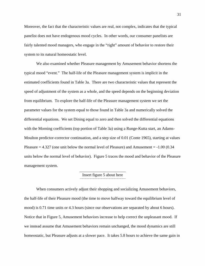
We also examined whether Pleasure management by Amusement behavior shortens the

typical mood “event.” The half-life of the Pleasure management system is implicit in the

estimated coefficients found in Table 3a. There are two characteristic values that represent the

speed of adjustment of the system as a whole, and the speed depends on the beginning deviation

from equilibrium. To explore the half-life of the Pleasure management system we set the

parameter values for the system equal to those found in Table 3a and numerically solved the

differential equations. We set Dining equal to zero and then solved the differential equations

with the Morning coefficients (top portion of Table 3a) using a Runge-Kutta start, an Adams-

Moulton predictor-corrector continuation, and a step size of 0.01 (Conte 1965), starting at values

Pleasure = 4.327 (one unit below the normal level of Pleasure) and Amusement = -1.00 (0.34

units below the normal level of behavior). Figure 5 traces the mood and behavior of the Pleasure

management system. _______________________

Insert figure 5 about here ⎯⎯⎯⎯⎯⎯⎯⎯⎯⎯⎯⎯⎯⎯⎯⎯⎯

When consumers actively adjust their shopping and socializing Amusement behaviors,

the half-life of their Pleasure mood (the time to move halfway toward the equilibrium level of

mood) is 0.71 time units or 4.3 hours (since our observations are separated by about 6 hours).

Notice that in Figure 5, Amusement behaviors increase to help correct the unpleasant mood. If

we instead assume that Amusement behaviors remain unchanged, the mood dynamics are still

homeostatic, but Pleasure adjusts at a slower pace. It takes 5.8 hours to achieve the same gain in

32

Pleasure that occurred in only 4.3 hours when behavior was managed in response to the mood.

In other words, consumers who don’t do anything to improve their moods (like shopping or

socializing) will still experience an improvement in mood because the natural homeostatic

system is at work; however, active mood managers will be in better moods 27% faster.

The increase in the speed of adjustment of mood depends, of course, on the initial

conditions of mood management. Since the behavior cannot change instantaneously, but rather

at the measured pace of its own dynamic, mood-management consumption can act either as a sail

or as an anchor depending on whether the starting behavior is high or low. If the mood

management system started very close to equilibrium, the speed of adjustment would necessarily

be very slow since not much change in mood is required to reach homeostasis.

Findings on Arousal Management

We only briefly discuss the Arousal mood management system because many of issues

are identical. Like pleasure dynamics, arousal dynamics also show strong indications of

homeostasis. The top row of the arousal dynamics matrix (enclosed in boxes in Table 3b)

indicates that the coefficient of Arousal as a determinant of the rate of change of Arousal is -α=-

1.26 (statistically significant at p < .01). This means that a person who is more excited than

normal naturally calms down over time. The negative characteristic values in Table 3b indicate

the strong homeostasis of the Arousal management system and that the equilibrium is stable.

There is no evidence of endogenous mood cycles.

Using the estimated coefficients for the Morning Arousal management system, the

numerical solution of the Arousal-Relaxation differential equations was calculated starting the

system 1.0 units below the equilibrium Arousal level and 0.34 units above on Relaxation

33

behavior (as was done above for the equivalent Pleasure-Amusement system). When active

mood management is allowed, the time needed for Arousal to close half the gap to equilibrium is

0.66 time units (3.9 hours). When Relaxation behaviors (watching television and listening to

music) are not allowed to change, it takes 1.15 time units (6.9 hours) to achieve an equal gain in

Arousal. Active management of Relaxation behaviors speed up Arousal adjustment by 42%.

Comparing the two mood dimensions, the half-life of Pleasure management (4.3 hours) is

10% longer than Arousal management (3.9 hours). This is consistent with the characteristic

values of the Arousal system which are slightly more negative than those of the Pleasure system.

Unhappiness drags on, but excitement disappears more rapidly.

Comparison of Estimates with Predicted Signs The critical prediction of the homeostatic mood-management system is that the

characteristic values given in equation (5) have negative real parts. We found this to be true for

all estimated models. Moreover, we found no indication that the mood-management system

resulted in endogenous mood cycles. The mood dynamics system may overshoot equilibrium

once, but then it steadily converges to equilibrium levels of mood and behavior.

Table 5 compares the theoretical predictions with the empirical findings in Tables 3 and

4. All the signs are in the predicted direction for α, β, and δ. All are statistically significant.

The predicted values of γ are supported roughly half the time, but afternoon behavior is

distinctly different than predicted. Dining’s influence on mood adjustment was insignificant.

_______________________ Insert Table 5 about here

⎯⎯⎯⎯⎯⎯⎯⎯⎯⎯⎯⎯⎯⎯⎯⎯⎯

34

DISCUSSION

This paper presents the first fully dynamic modeling of both mood and mood-managing

behavior in a naturally occurring setting. Our goal in designing and implementing this research

was to move past conceptual models of consumer mood management and further an empirical

understanding of the process of mood management.

The challenge addressed was to simultaneously model the psychological reaction of

mood to behaviors, but also to recognize and measure the relationship between mood and the

activities chosen specifically to manage the mood. Our basic theory was that the mood-

management system of interlinked, dual causation, mood and behavior followed a homeostatic

dynamic path. Since moods are transient feeling states by definition, we modeled the adjustment

of moods as occurring continuously over time. This operationalization of mood dynamics

presented difficulties because mood and mood-managing behaviors can at best be measured only

intermittently. We solved this dilemma by using continuous-time differential equations in our

model, and estimating cumulative mood and behavior using a double-trapezoidal approximation.

Through a two-stage least-squares estimation procedure, we were able to estimate the

interdependent effects of mood and behavior, and the time-path of mood and behavior to

equilibrium. With our model, we were able to explain about one-third of the period-to-period

changes in consumers’ moods and behaviors. The findings strongly supported the principle of

homeostasis as the dynamic process underlying the mood-management system.

Our continuous time model is superior to discrete time models used in previous research

in several ways. Mood is a phenomenon that changes over time and that continually interacts

with other dynamic aspects of the psychological system and the environment (Parkinson et al.

1996). Our model is a more authentic representation of mood and mood-management dynamics,

35

it provides information about the system at all times (rather than at discrete points in time), and it

can demonstrate the expected effects of a parameter or input value change to the system.

A panel of 93 adults was interviewed three times per day for five days to obtain measures

of mood and behavior. This intermittent data was then used to estimate the coefficients of the

continuous time mood-behavior process. Our method of empirically fitting continuous-time

models to intermittent data could be used to measure the differences between typical consumers

and compulsive consumers, for example, by changing the parameter value of the amount of

shopping behavior engaged in and the period-to-period changes in mood. Such a model also

may be of use in other marketing domains, such as consumer learning (Gregan-Paxton and

Roedder John 1997), adoption of innovations (Fisher and Price 1992), product diffusion models

(Bass, Krishnan, and Jain 1994; Kim et al. 1999), real-time customer satisfaction (Bolton and

Drew 1991; Dubé and Morgan 1998; Johnson, Anderson, and Fornell 1995), and the dynamics of

advertising persuasiveness (Baumgartner et al. 1997; Burke and Edell 1986).

The new substantive findings of this research include the following.

a. The full mood-management system (mood and behavior) is very stable, as predicted

by homeostasis.

b. Even without behavioral adjustments, mood is inherently stable.

c. The arousal dimension of mood returns 10% more rapidly to normal levels than does

the pleasure dimension of mood.

d. There is no indication of long endogenous mood cycles created by the effort to

manage moods.

e. The management of amusement behaviors (shopping and socializing) speeds up the

return of pleasure to normal levels by about 30%, while the management of relaxing

36

behaviors (watching TV and listening to music) speeds up the return of arousal to

normal levels by about 40%.

f. Mood management is somewhat slower in the afternoon and evening than in the

morning.

g. Media-oriented behavior (watching TV, listening to music) is more powerful and

homeostatic than socially-oriented consumer behavior (shopping, socializing) in

managing mood.

h. Dining out does not have a measurable effect on mood dynamics.

These findings have implications for consumer mood researchers and marketing

practitioners. Our results suggest that experimental designs that induce moods need to account

for the differential effects of stimuli that create pleasurable feelings and arousing feelings. The

longer-lasting mood effects of pleasure may impact dependent measures. Further, time-of-day

effects may impact experimental results and researchers may want to treat time-of-day as a

blocking variable in studies that manipulate mood.

That the media-oriented behavior (independent activities such as watching TV and

listening to music) is more effective than socially-oriented behavior (interdependent activities

such as shopping and socializing) has implications for service providers, as well as cross-cultural

researchers who explore individualist and collectivist consumer behaviors. Future research

might explore the effectiveness of various behaviors at prolonging or repairing a consumer’s

mood among different consumer segments.

Marketing practitioners also gain insight into consumers as a result of our study. The

longer lasting effects of a pleasurable mood experience compared to an exciting mood

experience suggest different “windows of opportunity” in which advertisers, service providers,

37

and retailers can benefit from consumers’ efforts at managing their moods. Arousal disappears

10% faster than pleasure, so advertising that is aimed at immediate behaviors may disappoint if

copy and execution focus on stimulating arousal, rather than on creating feelings of pleasure.

The fact that our model provides information about the mood-management system at all

times, as well as demonstrating the expected effects of a parameter or input value change to the

system means our model, with some modifications, can provide marketers valuable information

that will more directly help them to create more efficient and more effective advertising

campaigns, product offerings, or retail environments. Understanding how much (in terms of both

duration and degree) pleasing or arousing stimuli will be sought before consumers switch to less

pleasing or calming activities will help marketers of many products such as amusement parks,

media programs, retail entertainment centers (e.g., ESPN Zone) or tour packages to design better

product offerings with more appealing sequences of activities or programs that prolong

consumption time and enhance consumers’ experience.

We also recognize some limitations to this study. First, our panelists were only

interviewed every six hours. Our calculations tell us that the half-life of a mood episode is

between 4 and 6 hours, but more frequent observations of mood might capture more transient

mood states. Our data shows no evidence of endogenous mood cycles. However, the theory of

Nyquist sampling says that only if mood cycles had a length of twelve hours would our sample

intervals of six hours correctly identify the cycle (Nyquist 1928).12 We recognize that more

evidence is needed to determine the length of a typical naturally occurring mood cycle. On the

other hand, even given the generous time between mood and behavior measures in our study, we

can still explain a significant portion of the mood-management system.

12 We thank James Heyman, University of California-Berkeley, for this observation.

38

Second, some of the affective states measured in our panel study may be emotions rather

than moods; in some instances we may have captured displeasure focused at a coworker rather

than mood. As Clore et al. (2000, p. 30) said, “It is useful to think of emotions as affective

states with objects and moods as affective states without objects. But it is important to recognize

that emotions act like moods when their object states are not focal [italics added].” Bagozzi,

Gopinath, and Nyer (1999, p. 184) said, “The line between an emotion and mood is frequently

difficult to draw but often by convention involves conceiving of a mood as being longer lasting

(from a few hours up to days) and lower in intensity than an emotion.” Given the short-run

nature of such emotion states (as Bagozzi et al. implies) it is probable that any emotion

experienced by our panelists was diffused into the background and was without a direct object

focus (as Clore et al. implies) at the time of the interview. For example, if the displeasure at a

coworker occurred fifteen minutes before our telephone interview, the panelist may have

retained the affect, but lost the focus on the coworker during the interview. Therefore, the affect

we measured is more likely mood rather than emotion, in this technical sense.

Third, behaviors have a host of driving forces other than mood (or time of day) and these

other factors should be measured and accounted for in future research. The authenticity of field

research leaves one with the dilemma that other relevant but unmeasured variables get swept into

the error term. Sixty to seventy percent of behavior is left unexplained in our model estimation.

If other variables not included in the model are correlated with some of our independent

variables, then a confound exists. We might be interpreting a coefficient as the influence of

relaxation behavior on changes in arousal, when it is really caused by an auto accident on the

way home from work, a telephone call from an old friend, or some other unmeasured event. All

such events admittedly can cause substantial adjustments to moods, but unless there is a strong

39

correlation between these events and the other included variables, no bias exists in estimates of

the other coefficients. We do believe that there may be events that occur on a regular schedule

that affect mood and behavior, and we have used the time-of-day (morning, afternoon, evening)

variable to act as a proxy for them in our model.

Fourth, each night our panelists went to sleep. Certainly sleep must have a pronounced

effect on moods as well as on cumulative behaviors (or the recollection of those behaviors) but

our model does not account for the effects of sleep on mood or behavior. We look forward to

other studies that might guide methods of incorporating sleep interruptions in continuous time

events.

Fifth, we only interviewed panelists Monday through Friday. What about weekends? A

longer longitudinal study would help to improve our understanding of mood dynamics by

accounting for day-of-week effects or other seasonalities. For example, research indicates that

between 92 and 95% of the U.S. general population demonstrate seasonal mood and behavior

changes characteristic of Seasonal Affective Disorder (Spoont, Depue, and Krauss 1991). A

longer mood study might provide some valuable insights into the dynamics of S.A.D.

Sixth, the estimated coefficients of the mood dynamics system come from a pooled data

set that treats all subjects as essentially identical in the across-subjects study (see footnote 9).

There is a common but controversial belief that women are more emotional than men, and some

psychological studies do indicate that women are more prone than men to depression and

depressive moods (Weissman and Klerman 1977). Other studies have shown that men have

greater physiological reactivity to stress than do women (Gottman and Levenson 1988). These

findings suggest the possibility of sex differences in the dynamics of mood-management.

40

We tested whether males and females have identical mood-management systems (details

available upon request from the authors) and found that for all the mood or behavior equations

the fit was improved when the coefficients of males and females were allowed to differ.

However, with only 29 males and 64 females it was difficult to distinguish the sexes on all

parameters. We found that men’s mood adjustments are more responsive to behavior than are

women’s. In addition, when a woman’s Pleasure is pushed above or below its equilibrium level

by outside events, she will naturally adjust mood and Amusement behaviors (shopping and

socializing) to return more quickly than a man to the equilibrium level of Pleasure. On the other

hand, men’s Arousal management system is more homeostatic than women’s. Future research

might explore further the differences between men’s and women’s mood-management systems,

or incorporate other demographic and psychographic variables into the model, such as age or

affective responsiveness (Larsen and Diener 1987).

A major challenge facing marketing academics and practitioners is to understand the

dynamics of consumer mood management, to analyze the products and behaviors that consumers

use to regulate their mood states, and to design marketing programs that are responsive to the

needs of consumers seeking to maintain or to change their moods. This requires that the

characteristics of consumers’ mood states and their mood-management behaviors be identified

and measured, and the dynamic process by which moods and behaviors adjust be described and

modeled. We hope that this study has furthered these goals.

41

REFERENCES

Bagozzi, Richard P., Mahesh Gopinath, Prashanth U. Nyer (1999), “The Role of Emotions in

Marketing,” Journal of the Academy of Marketing Science, 27 (Spring), 184-206.

Barone, Michael J., Paul W. Miniard, and Jean B. Romeo (2000), “The Influence of Positive

Mood on Brand Extension Evaluations,” Journal of Consumer Research, 26 (March), 386-400.

Bass, Frank, Trichy Krishnan, and Dipak Jain (1994), “Why the Bass Model Fits Without

Decision Variables,” Marketing Science, 13 (Summer), 203-223.

Batra, Rajeev and Douglas M. Stayman (1990), “The Role of Mood in Advertising

Effectiveness,” Journal of Consumer Research, 13 (September), 203-214.

Baumgartner, Hans, Mita Sujan, and Dan Padgett (1997), “Patterns of Affective Reactions to

Advertisements: The Integration of Moment-to-Moment Responses into Overall Judgments,”

Journal of Marketing Research, 34 (May), 219-232.

Bergstrom, Albert R., ed. (1976), Statistical Inference in Continuous Time Economic Models,

Amsterdam: North-Holland.

______________ (1993), “The History of Continuous-Time Econometric Models,” in

Continuous-Time Econometrics Theory and Applications, ed. Giancarlo Gandolfo, London:

Chapman & Hall, 13-34.

Berntson, Gary G. and John T. Cacioppo (2000), “From Homeostasis to Allodynamic

Regulation,” in Handbook of Psychophysiology, ed. John T. Cacioppo and Louis G. Tassinary,

New York: Cambridge University Press, 459-481.

Bolton, Ruth N. and James H. Drew (1991), “A Multistage Model of Customers’ Assessments of

Service Quality and Value,” Journal of Consumer Research, 17 (March), 375-384.

42

Bryant, Jennings and Dolf Zillmann (1984), “Using Television to Alleviate Boredom and Stress:

Selective Exposure as a Function of Induced Excitational States,” Journal of Broadcasting, 28

(Winter), 1-20.

Burke, Marian Chapman and Julie A. Edell (1986), “Ad Reactions over Time: Changes in the

Real World,” Journal of Consumer Research, 13 (June), 114-118.

Canon, Walter B. (1932), The Wisdom of the Body, New York: Norton.

Clore, Gerald L., Robert S. Wyer, Jr., Bruce Dienes, Karen Gasper, Carol Gohm, and Linda

Isabell (2000), “Affective Feelings as Feedback: Some Cognitive Consequences,” in Theories

of Mood and Cognition: A Users Handbook, ed. Gerald Clore and Leonard L. Martin,

Mahwah, NJ: Erlbaum, 27-62.

Cohen, Joel B. and Charles S. Areni (1991), “Affect and Consumer Behavior,” in Handbook of

Consumer Behavior, ed. Thomas S. Robertson and Harold H. Kassarjian, Englewood Cliffs,

NJ: Prentice-Hall, 188-240.

Conte, Samuel D. (1965), Elementary Numerical Analysis: An Algorithmic Approach, New York:

McGraw-Hill.

Csikszentmihalyi, Mihaly, and Robert Kubey (1981), “Television and the Rest of Life: A

Systematic Comparison of Subjective Experience,” Public Opinion Quarterly, 45, 317-328.

Diener, Ed and Robert A. Emmons (1984), “The Independence of Positive and Negative Affect,”

Journal of Personality and Social Psychology, 47 (November), 1105-1117.

____________, Randy J. Larsen, Steven Levine, and Robert A. Emmons (1985), “Intensity and

Frequency: Dimensions Underlying Positive and Negative Affect,” Journal of Personality and

Social Psychology, 48 (May), 1253-1265.

43

Dubé, Laurette, Jean-Charles Chebat, and Sylvie Morin (1995), “The Effects of Background

Music on Consumers’ Desire to Affiliate in Buyer-Seller Interactions,” Psychology and

Marketing, 12 (July), 305-319.

____________ and Michael S. Morgan (1998), “Capturing the Dynamics of In-process

Consumption Emotions and Satisfaction in Extended Service Transactions,” International

Journal of Research in Marketing, 15, 309-320.

Edlund, Matthew (1987), Psychological Time and Mental Illness, New York: Gardner.

Eliashberg, Jehoshua and Mohanbir S. Sawhney (1994), “Modeling Goes to Hollywood:

Predicting Individual Differences in Movie Enjoyment,” Management Science, 40

(September), 1151-1173.

Faber, Ronald J. and Gary A. Christenson (1996), “In the Mood to Buy: Differences in the Mood

States Experienced by Compulsive Buyers and Other Consumers,” Psychology and Marketing,

13 (December), 803-819.

Fisher, Robert J. and Linda L. Price (1992), “An Investigation into the Social Context of Early

Adoption Behavior,” Journal of Consumer Research, 19 (December), 477-486.

Gandolfo, Giancarlo, ed. (1993), Continuous-Time Econometrics: Theory and Applications,

London: Chapman & Hall.

Gardner, Meryl P. (1985), “Mood States and Consumer Behavior: A Critical Review,” Journal of

Consumer Research, 12 (December), 281-300.

Goldstein, Patrick (1993), “Shaquille O’Neal, A Celebrity for the New World,” Rolling Stone,

November 25, 52 –58, 133-134.

44

Gottman, John M. and Robert W. Levenson (1988), “The Social Psychophysiology of Marriage,”

in Perspectives on Marital Interaction, ed. Patricia Noller and Mary Anne Fitzpatrick,

Philadelphia, PA: Multilingual Matters, 182-200.

Green, Donald and Peter Salovey (1999), “In What Sense Are Positive and Negative Affect

Independent? A Reply to Tellegen, Watson, and Clark,” Psychological Science, 10 (July), 304-

306.

Gregan-Paxton, Jennifer, and Deborah Roedder John (1997), “Consumer Learning by Analogy: A

Model of Internal Knowledge Transfer,” Journal of Consumer Research, 24 (December), 266-

284.

Headey, Bruce and Alexander Wearing (1989), “Personality, Life Events, and Subjective Well-

Being: Toward a Dynamic Equilibrium Model,” Journal of Personality and Social Psychology,

57, 731-739.

Holbrook, Morris B. and Meryl P. Gardner (2000), “Illustrating a Dynamic Model of the Mood-

Updating Process in Consumer Behavior,” Psychology and Marketing, 17 (March), 165-194.

_______________ and Elizabeth C. Hirschman (1982), “The Experiential Aspects of

Consumption: Consumer Fantasies, Feelings, and Fun, Journal of Consumer Research, 9

(September), 132-140.

Isen, Alice (1984), “Toward Understanding the Role of Affect in Cognition,” in Handbook of

Social Cognition, ed. Robert Wyer, Jr. and Thomas Srull, Hillsdale, NJ: Erlbaum, 179-236.

Johnson, Michael D., Eugene W. Anderson, and Claes Fornell (1995), “Rational and Adaptive

Performance Expectations in a Customer Satisfaction Framework,” Journal of Consumer

Research, 21 (March), 695-707.

45

Kacen, Jacqueline J. (1994), “Phenomenological Insights into Moods and Mood-related

Consumer Behaviors,” Advances in Consumer Research, Vol. 21, ed. Chris T. Allen and

Deborah Roedder John, Provo, UT: Association for Consumer Research, 519-525.

_____________ and Julie A. Lee (2002) “The Influence of Culture on Consumer Impulsive

Buying Behavior,” Journal of Consumer Psychology, 12 (March), 163-176.

Kim, Namwoon, Eileen Bridges, and Rajendra K. Srivastava (1999), “A Simultaneous Model for

Innovative Product Category Sales Diffusion and Competitive Dynamics,” International

Journal of Research in Marketing, 16, 95-111.

Larsen, Randy J. (2000), “Toward a Science of Mood Regulation,” Psychological Inquiry, 11 (3),

129-141.

____________ and Ed Diener (1987), “Affect Intensity as an Individual Difference

Characteristic: A Review,” Journal of Research in Personality, 21 (March), 1-39.

_____________ and Timothy Ketelaar (1991), “Personality and Susceptibility to Positive and

Negative Emotional States,” Journal of Personality and Social Psychology, 61 (July), 132-140.

Lee, Angela Y. and Brian Sternthal (1999), “The Effects of Positive Mood on Memory,” Journal

of Consumer Research, 26 (September), 115-127.

Luomala, Harri T. (1999), “A Qualitative Exploration of Mood-regulatory Self-gift Behaviors,”

Journal of Economic Psychology, 20 (April), 147-182.

Mano, Haim and Richard L. Oliver (1993), “Assessing the Dimensionality and Structure of the

Consumption Experience: Evaluation, Feeling, and Satisfaction,” Journal of Consumer

Research, 20 (December), 451-466.

Morris, William N. and Nora P. Reilly (1987), “Toward the Self-Regulation of Mood: Theory and

Research,” Motivation and Emotion, 11 (September), 215-249.

46

Nyquist, Harry (1928), “Certain Topics in Telegraph Transmission Theory,” American Institute of

Electrical Engineers Transactions, 47 (April), 617.

Parker, Philip M. and Nader T. Tavassoli (2000), “Homeostasis and Consumer Behavior Across

Cultures,” International Journal of Research in Marketing, 17, 33-53.

Parkinson, Brian, Peter Totterdell, Rob B. Briner, Shirley Reynolds (1996), Changing Moods:

The Psychology of Mood and Mood Regulation, New York: Longman.

Phillips, Peter C. B. (1974), “The Estimation of Some Continuous Time Models,” Econometrica,

42, 802-824.

Russell, James A. (1980), “A Circumplex Model of Affect,” Journal of Personality and Social

Psychology, 39 (December), 1161-1178.

_____________ and George Pratt (1980), “A Description of the Affective Quality Attributed to

Environments,” Journal of Personality and Social Psychology, 38 (August), 311-322.

_____________, Anna Weiss, and Gerald A. Mendelsohn (1989), “Affect Grid: A Single-Item

Scale of Pleasure and Arousal,” Journal of Personality and Social Psychology, 57

(September), 493-502.

Samuelson, Paul A. (1947), The Foundations of Economic Analysis, Cambridge: Harvard

University Press.

Schulze, Georg (1995), “Motivation: Homeostatic Mechanisms May Instigate and Shape

Adaptive Behaviors Through Generation of Hedonic States,” in Biological Perspectives on

Motivated Activities, ed. Roderick Wong, Stamford, CT: Ablex, 265-288.

Spoont, Michele R., Richard A. Depue, and Steven S. Krauss (1991), “Dimensional Measurement

of Seasonal Variation in Mood and Behavior,” Psychiatry Research, 39 (December), 269-284.

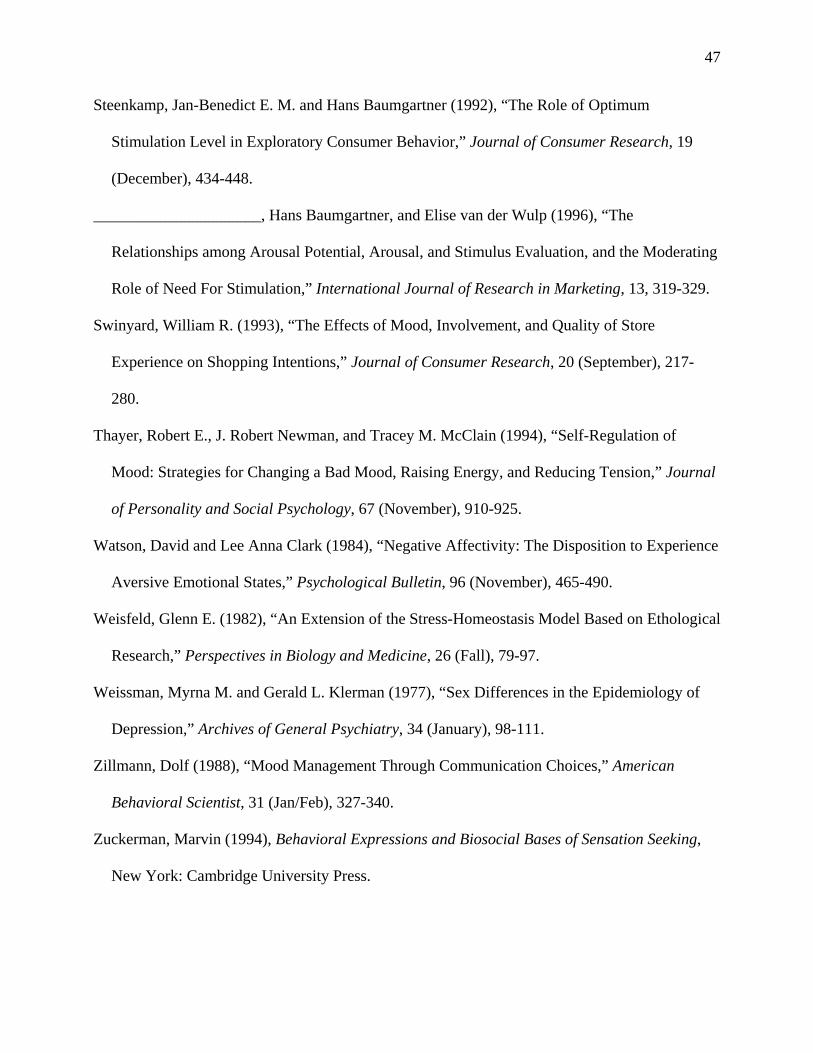
47

Steenkamp, Jan-Benedict E. M. and Hans Baumgartner (1992), “The Role of Optimum

Stimulation Level in Exploratory Consumer Behavior,” Journal of Consumer Research, 19

(December), 434-448.

_____________________, Hans Baumgartner, and Elise van der Wulp (1996), “The

Relationships among Arousal Potential, Arousal, and Stimulus Evaluation, and the Moderating

Role of Need For Stimulation,” International Journal of Research in Marketing, 13, 319-329.

Swinyard, William R. (1993), “The Effects of Mood, Involvement, and Quality of Store

Experience on Shopping Intentions,” Journal of Consumer Research, 20 (September), 217-

280.

Thayer, Robert E., J. Robert Newman, and Tracey M. McClain (1994), “Self-Regulation of

Mood: Strategies for Changing a Bad Mood, Raising Energy, and Reducing Tension,” Journal

of Personality and Social Psychology, 67 (November), 910-925.

Watson, David and Lee Anna Clark (1984), “Negative Affectivity: The Disposition to Experience

Aversive Emotional States,” Psychological Bulletin, 96 (November), 465-490.

Weisfeld, Glenn E. (1982), “An Extension of the Stress-Homeostasis Model Based on Ethological

Research,” Perspectives in Biology and Medicine, 26 (Fall), 79-97.

Weissman, Myrna M. and Gerald L. Klerman (1977), “Sex Differences in the Epidemiology of

Depression,” Archives of General Psychiatry, 34 (January), 98-111.

Zillmann, Dolf (1988), “Mood Management Through Communication Choices,” American

Behavioral Scientist, 31 (Jan/Feb), 327-340.

Zuckerman, Marvin (1994), Behavioral Expressions and Biosocial Bases of Sensation Seeking,

New York: Cambridge University Press.

48

Table 1: General Description of Panelists

Entire Sample (N=93: 1395 total observations)

Age Mean 38.9 Occupation Managerial 20.4% (years) Range 21-73 Professional 37.6%

Non-manual skilled 19.4% Gender Male 31 % Manual skilled 6.5%

Female 69 % Partly- or unskilled 1.1% Unemployed 6.5%

Marital Status Single or Divorced 41.9 % Other 8.6% Married 58.1 % Education Some high school 1.1%

Income Under $15,000 5.4% High school 10.8% $15,000-$24,999 7.5% Some college 21.5% $25.000-$49,999 28.0% Undergraduate degree 39.8% $50,000-$74,999 19.4% Graduate degree 23.7% $75,000-$99,999 14.0% Ph.D. 3.2% $100,000 & above 25.8%

Household Size Mean 2.3 Range 1-5

49

Table 2: Behavior Classification System

Category Variables Measures

Item 1 Item 2 Item 3 Shop Time Number items Dollars spent

Amusement Socialize with others Time Private-Public* Number people Watch TV Time Involvement* Subject matter*

Relaxation Listen to music Time Tempo*(r) Variety* Dining Eat out Time Quality* Dollars spent

* Measured on a 7-point scale where 7 indicates higher or more seriously engaging level/value. (r) indicates reverse-coded item.

50

Table 3 Two Stage Least Squares Estimates (t-statistics)

a. Pleasure Management in Morning

Variables

Derivatives of Mood/ Behavior

Pleasure Mood

Amusement Behavior a

Dining Intercept R2 c

Pleasuredt

d -1.11***

(-14.72) 0.78***

(3.80) -.07

(-1.36) 6.43***

(14.48) 0.30

Amusementdt

d

-0.18**, b

(2.58) -2.17***

(-16.21) -0.48

(-1.21) 0.36

Characteristic

valuesd -1.29*** -1.98***

(-8.43) (-9.57)

.b. Arousal Management in Morning

Variables

Derivatives of Mood/ Behavior

Arousal Mood

Relaxation Behaviore

Dining Intercept R2 c

Arousaldt

d -1.26***

(-13.60) -1.29***

(-6.19) -.02

(-0.32) 6.32***

(13.08) 0.35

laxationRedt

d 0.20**, b

(2.40) -2.69***

(-16.92) -0.10

(-0.27) 0.39

-1.51*** -2.44*** Characteristic valuesd (-7.86) (-9.75)

* Significant at 10%, ** Significant at 5%, *** Significant at 1%, N=1170 a Amusement behaviors are shopping and socializing. b The coefficient for the Morning. This coefficient varies by time-of-day as seen in Table 7. c R2 is calculated as SSR/(SSR+SSE) with both regression and error sum of squares calculated using the

estimated coefficients and the actual values of explanatory variables.d Solutions are linear combinations of exp(at), where a is a characteristic value of the dynamics matrix

(found in the box). Statistics for a were computed using a Monte Carlo simulation of 1000 values of the dynamics matrix drawn from a distribution with its estimated mean and standard error.

e Relaxation behaviors are watching television and listening to music.

51

Table 4 Two Stage Least Squares Estimates (t-statistics)a

a. Amusement Dynamics by Time-of-Day

Variables

Derivatives of Behavior

Amusementdt

d

Pleasure Mood

Amusement Behavior b

Characteristic valuesc

-1.29*** -1.98*** Morning -0.18** † (2.58)

-2.17*** (-16.21) (-8.43) (-9.57)

-1.01*** -2.26*** Afternoon 0.15** † (2.02) “ (-11.15) (-16.99)

-0.94*** -2.33*** Evening 0.27*** † (3.62) “ (-10.48) (-17.63)

b. Relaxation Dynamics by Time-of-Day

Variables

Derivatives of Behavior

laxationRedt

d

Arousal Mood

Relaxation Behavior d

Characteristic valuesc

-1.51*** -2.44*** Morning 0.20** †† (2.40)

-2.69*** (-16.92) (-7.86) (-9.75)

-0.97*** -2.98*** Afternoon -0.39*** † (-4.76) “ (-9.17) (-19.65)

-1.40*** -2.55** Evening 0.13* †† (1.75) “ (-9.82) (-12.41)

* Significant at 10%, ** Significant at 5%, *** Significant at 1%, N=1170 † The coefficient for this time-of-day is different from the coefficients at other times at 1%. †† Morning and evening coefficients are not different statistically, but are different from the afternoon

coefficient at 1%. a The remainder of the mood-management statistics are identical to those of Table 5. b Amusement behaviors are shopping and socializing. c Solutions are linear combinations of exp(at), where a is a characteristic value of the dynamics matrix (found in the box). Statistics for a were computed using a Monte Carlo simulation of 1000 values of the dynamics matrix drawn from a distribution with its estimated mean and standard error. d Relaxation behaviors are watching television and listening to music.

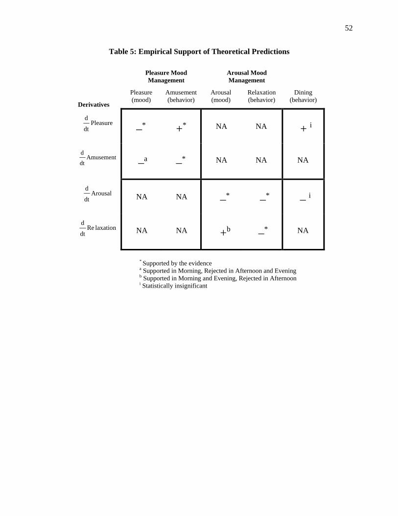
52

Table 5: Empirical Support of Theoretical Predictions

Pleasure Mood Management

Arousal Mood Management

Derivatives

Pleasure (mood)

Amusement (behavior)

Arousal (mood)

Relaxation (behavior)

Dining (behavior)

Pleasuredt

d

–*

+*

NA

NA

+ i

Amusementdt

d

–a

–*

NA

NA

NA

Arousaldt

d

NA

NA

–*

–*

– i

laxationRedt

d

NA

NA

+b

–*

NA

* Supported by the evidence a Supported in Morning, Rejected in Afternoon and Evening b Supported in Morning and Evening, Rejected in Afternoon i Statistically insignificant

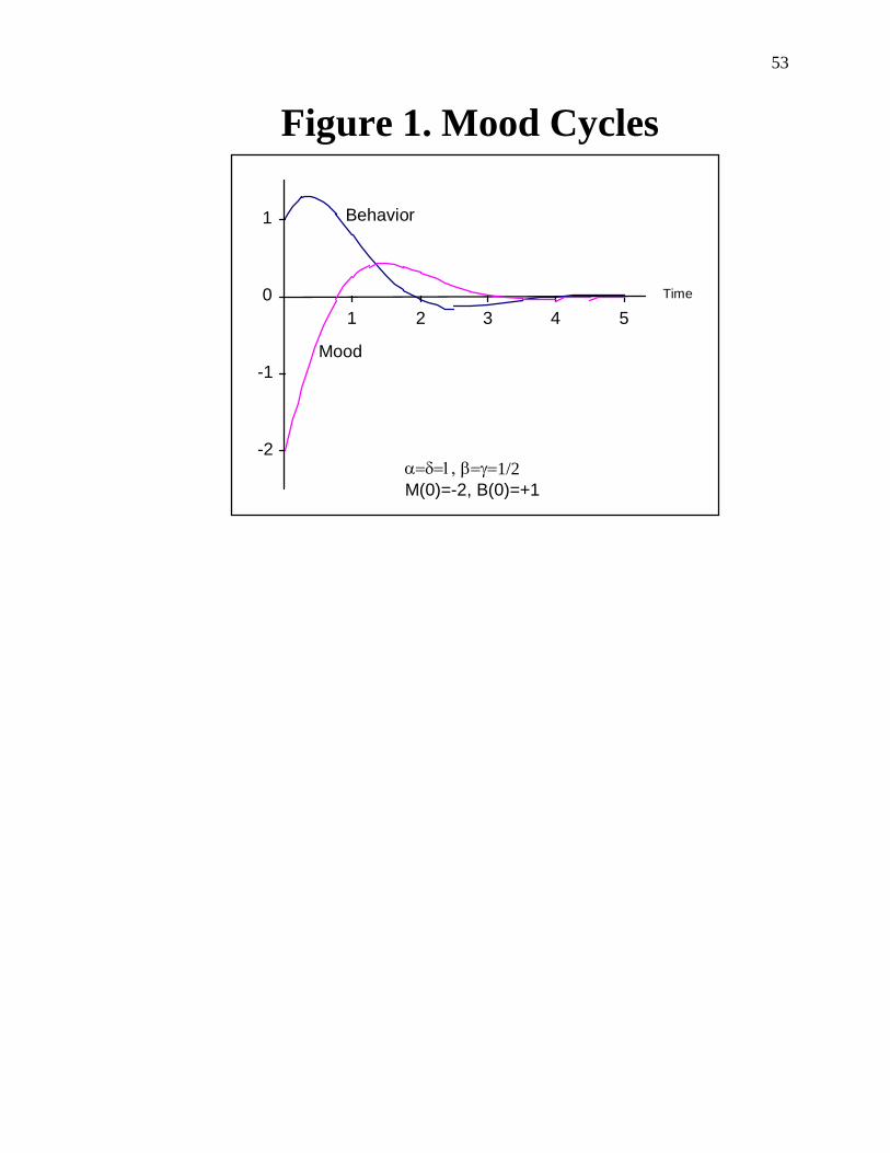
53

α=δ=1, β=γ=1/2M(0)=-2, B(0)=+1

-2

-1

0

1

1 2 3 4 5

Behavior

Mood

Time

Figure 1. Mood Cycles

54

Figure 2. Influence of Activities on Pleasure and Arousal(Preliminary Survey)

0.0

1.0

2.0

3.0

4.0

5.0

6.0

7.0

0.0 2.0 4.0 6.0 8.0

Shop

Eat Out

Socialize

TV

Music

Pleasure

Arousal

Mean of other items

Mean ofotheritems

55

ti-1 ti

M(t)

t

M(ti-1)

M(ti)

Figure 3. Trapezoid Approximationof Cumulative Mood

56

ti-1 ti

B(t)

t

i-1B(t )

B(t i)

tI+1ti-2

i+1B(t )

I

JK

LV

U

i-1+tti-22

i+tti-12

i+1+tti2

C D E

Figure 4. Double TrapezoidApproximation of Cumulative Behavior

57

4.2

4.4

4.6

4.8

5.0

5.2

≈

≈Time (hours)

Pleasure returnshalfway to equilibrium

Pleasure (with activeAmusement behavior)

managed Amusementbehavior

Figure 5. Solution of Pleasure-AmusementDifferential Equations (Morning)

Beginning Below Equilibrium

4.3 5.8

-1.0

-0.6

Pleasure (with constant Amusement behavior)

constant Amusementbehavior

Pleasure half-life is reduced 27%by Amusement management