Monte Carlo Simulations of Weapon Effectiveness …€”Carleton damage function has been commonly ... multiple shots of an unguided artillery weapon against an area target was chosen

Abstract—Carleton damage function has been commonly

utilized to describe the weapon-target interaction in the weapon

effectiveness analyses. This function is simplified from the

actual weapon lethality data and these simplifications can affect

the analysis results. This paper investigates the difference

between results of Monte Carlo simulations to determine the

probability of target damage that utilize the Carleton damage

function and the results of the same simulations that utilize a

non-simplified probability of kill (Pk) matrix. A problem of

multiple shots of an unguided artillery weapon against an area

target was chosen as a case study. Two sets of Monte Carlo

simulations to determine the probability of damage on a target

were performed for several numbers of shots and target sizes.

The first set of simulations utilized the Pk matrix while the

second set utilized the Carleton damage function. Statistical

analyses were performed. It was suggested that there was

difference between the results of two sets of simulations but the

effect size was small.

Index Terms—Damage function, probability of damage,

Monte Carlo simulation, weapon effectiveness.

I. INTRODUCTION

Monte Carlo methods have been employed in the field of

weapon effectiveness to determine the probability of target

damage when there are no close form solutions available. A

Monte Carlo simulation to determine the probability of

damage on an area target inflicted by artillery weapons

normally comprises several thousand runs. In each run, the

impact points of all shots are randomized in accordance with

the weapon delivery accuracy. Then the probability of

damage inflicted by the weapons on the targets in each run

can be evaluated per weapon lethality data, which describe

the interaction between a specific weapon and a specific type

of targets. These weapon lethality data are normally

determined by testing or numerical simulation. They are

often presented in the form of Pk (Probability of kill) matrix

that describes Pk value at various distances around the impact

point. This format may be too complicated for computing in

the operations so the lethality data are approximated and

replaced by closed form damage functions.

Several damage functions have been described in many

literatures and text books [1]-[5]. Two most widely used

damage functions are the cookie cutter function and the

Carleton function. The cookie cutter function simply assumes

that fraction of the targets that lies inside the weapon lethal

area will be completely destroyed while the rest will receive

no damage. The Carleton function assumes Gaussian

distribution of Pk value at any distance from the impact point.

An example of recent research works that employed these

damage functions in Monte Carlo simulations to analyze

weapon effectiveness is Anderson [6]. In his work, Monte

Carlo simulations were performed to determine the

probability of damage inflicted on a point and an area target

by a single and a stick of air-to-surface weapons. The

simulations utilized the rectangular cookie cutter and the

Carleton function. The results from the Monte Carlo

simulations were compared to the results from JMEM (Joint

Munitions Effectiveness Manuals) method, which is a

standardized methodology developed by JTCG/ME (Joint

Technical Coordinating Group for Munitions Effectiveness)

in the United States of America [7].

In most cases of fragmentation weapons against personnel

targets, the Carleton function is apparently more realistic than

the cookie cutter function in representing the weapon

lethality. However, the Carleton function still differs from the

non-simplified Pk matrix and it can possibly affects the

results of Monte Carlo simulations. The objective of this

paper is to investigate whether the results of Monte Carlo

simulations that utilize the Carleton function differ from the

simulations that utilize a non-simplified Pk matrix. The focus

of this paper is on the problem of multiple shots of unguided

artillery weapon against a uniform value area target.

II. MONTE CARLO SIMULATION TO DETERMINE THE

PROBABILITY OF DAMAGE

A Monte Carlo method can refers to a computing

technique that determines results from many repeating

random sampling. Scientists who involved in the United

States nuclear project during World War II are often regarded

as the inventors of the Monte Carlo method [8], [9]. The

method is very useful when it is difficult or impossible to

obtain closed form solutions. This method has been

successfully applied to many scientific problems including

the weapon effectiveness and target coverage topics. In most

applications, Monte Carlo simulations are carried out by

computer programs for computing speed.

Monte Carlo Simulations of Weapon Effectiveness Using

Pk Matrix and Carleton Damage Function

Pawat Chusilp, Weerawut Charubhun, and Pattadon Koanantachai

International Journal of Applied Physics and Mathematics, Vol. 4, No. 4, July 2014

280DOI: 10.7763/IJAPM.2014.V4.299

Manuscript received May 2, 2014; revised July 2, 2014.

Pawat Chusilp, Weerawut Charubhun, and Pattadon Koanantachai are

with Defence Technology Institute, 47/433 Changewattana Road, Pakkred,

Nonthaburi 11120, Thailand (e-mail: [email protected],

[email protected], [email protected]).

From the next section, the paper is outlined as follows.

Section II briefly explains the calculation steps in a Monte

Carlo simulation to determine the probability of damage for

multiple shots against area targets. Section III describes the

Carleton damage function and how its parameters are

determined. Section IV describes a case study. The results are

presented and discussed in Section V. Section VI summarizes

the paper.

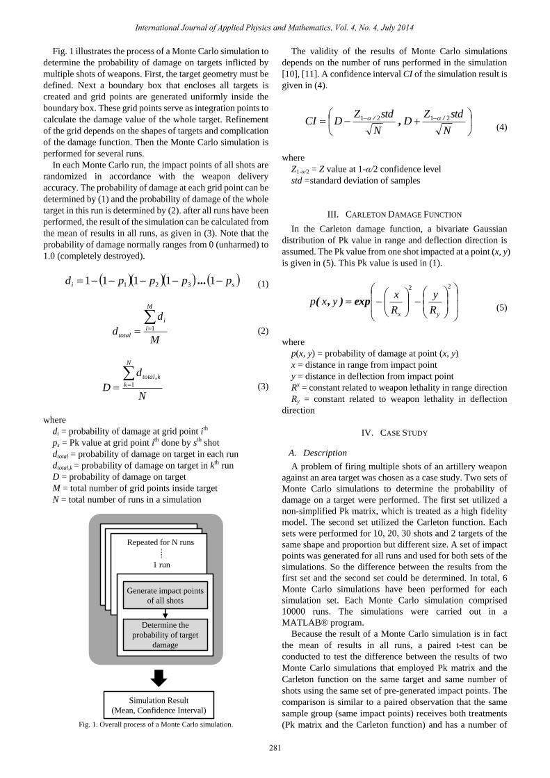
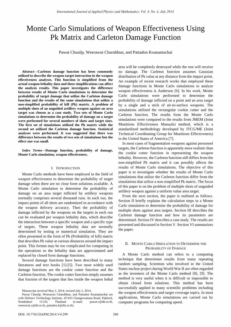
Fig. 1 illustrates the process of a Monte Carlo simulation to

determine the probability of damage on targets inflicted by

multiple shots of weapons. First, the target geometry must be

defined. Next a boundary box that encloses all targets is

created and grid points are generated uniformly inside the

boundary box. These grid points serve as integration points to

calculate the damage value of the whole target. Refinement

of the grid depends on the shapes of targets and complication

of the damage function. Then the Monte Carlo simulation is

performed for several runs.

In each Monte Carlo run, the impact points of all shots are

randomized in accordance with the weapon delivery

accuracy. The probability of damage at each grid point can be

determined by (1) and the probability of damage of the whole

target in this run is determined by (2). after all runs have been

performed, the result of the simulation can be calculated from

the mean of results in all runs, as given in (3). Note that the

probability of damage normally ranges from 0 (unharmed) to

1.0 (completely destroyed).

si ppppd 11111 321 ... (1)

M

d

d

M

i

i

total

1

(2)

N

d

D

N

k

ktotal 1

,

(3)

where

Run #2

Simulation Result

(Mean, Confidence Interval)

Repeated for N runs

Run #1

Generate impact points

of all shots

Determine the

probability of target

damage

1 run

……

Fig. 1. Overall process of a Monte Carlo simulation.

The validity of the results of Monte Carlo simulations

depends on the number of runs performed in the simulation

[10], [11]. A confidence interval CI of the simulation result is

given in (4).

N

stdZD

N

stdZDCI 2121 // ,

(4)

where

Z1-α/2 = Z value at 1-α/2 confidence level

std = standard deviation of samples

III. CARLETON DAMAGE FUNCTION

In the Carleton damage function, a bivariate Gaussian

distribution of Pk value in range and deflection direction is

assumed. The Pk value from one shot impacted at a point (x, y)

is given in (5). This Pk value is used in (1).

22

yx R

y

R

xyxp exp),(

(5)

x = distance in range from impact point

y = distance in deflection from impact point

Rx = constant related to weapon lethality in range direction

Ry = constant related to weapon lethality in deflection

direction

IV. CASE STUDY

A. Description

A problem of firing multiple shots of an artillery weapon

against an area target was chosen as a case study. Two sets of

Monte Carlo simulations to determine the probability of

damage on a target were performed. The first set utilized a

non-simplified Pk matrix, which is treated as a high fidelity

model. The second set utilized the Carleton function. Each

sets were performed for 10, 20, 30 shots and 2 targets of the

same shape and proportion but different size. A set of impact

points was generated for all runs and used for both sets of the

simulations. So the difference between the results from the

first set and the second set could be determined. In total, 6

Monte Carlo simulations have been performed for each

simulation set. Each Monte Carlo simulation comprised

10000 runs. The simulations were carried out in a

MATLAB® program.

Because the result of a Monte Carlo simulation is in fact

the mean of results in all runs, a paired t-test can be

conducted to test the difference between the results of two

Monte Carlo simulations that employed Pk matrix and the

Carleton function on the same target and same number of

shots using the same set of pre-generated impact points. The

comparison is similar to a paired observation that the same

sample group (same impact points) receives both treatments

(Pk matrix and the Carleton function) and has a number of


281

di = probability of damage at grid point ith

ps = Pk value at grid point ith done by sth shot

dtotal = probability of damage on target in each run

dtotal,k = probability of damage on target in kth run

D = probability of damage on target

M = total number of grid points inside target

N = total number of runs in a simulation

where

p(x, y) = probability of damage at point (x, y)

pairs of observations (probability of damage on target in each

run). Totally, 6 paired t-tests have been performed in the case

study.

Let μ1 be the result of a Monte Carlo simulation that

employs the Pk matrix, μ2 be the result of a Monte Carlo

simulation that employs the Carleton function, μd be the mean

of the difference between the paired results, which is equal to

μ1 – μ2 since the observations are paired. The following null

hypothesis H0 and alternative hypothesis H1 were tested at the

0.01 significance level.

H0: μd = 0

H1: μd ≠ 0

B. Weapon

A weapon chosen for the case study was a research

fragmentation warhead. Fig. 2 presents the contour of the Pk

matrix of the weapon when the detonation point is at (0, 0).

Only half of the figure is presented because the figure is

symmetrical about the range axis. The lethal area AL of the

warhead was calculated by (6), as defined in several

literatures [3], [5], [6]. Note that p(x, y) is the probability of

kill at a point(x,y), which is used in (1). Because the

resolution of the grid could affect the value of the lethal area

calculated by (6), a grid refinement study was carried out. It

was found that the value of lethal area approached 6192 m2

and a grid size of 0.6 m is appropriate for the simulations.

y x

L

yxyxp

dxdyyxpA

),(

),(

(6)

Fig. 2. Lethality of the warhead by Pk matrix.

C. Parameters of Carleton Function

The constants of the Carleton damage function could be

determined by applying a regression technique [12] on the

data in the Pk matrix. But for the two parameters Carleton

function employed in this paper, Rx and Ry were simply

determined by a guideline described in Driels [6]. The key

points are that the lethal area must be conserved and a ratio a

between Rx and Ry is a function of impact angle I as given in

(7). In all simulations, Rx = 24.87 m and Ry = 80.97 m were

used.

Ia cos.,.max 80130 (7)

In the simulations, all grid points located outside an ellipse,

of which the center is at the impact point and the major and

minor axes are 6Rx and 6Ry, were neglected because the Pk

value would be very small. A grid refinement study was also

conducted to ensure that the lethal area, as given in (6),

calculated by the Carleton function is equal the lethal area

calculated by Pk matrix. In addition, it was found that the

Carleton function actually required much coarser grid size,

and hence much less calculation time. But to eliminate any

effect on the results caused by different grid size, the same

grid size of 0.6 m was used in both simulations that employed

Pk matrix and the Carleton function.

D. Targets

The targets in the case study were a rectangular area

orientated at 30° from the range axis as shown in Fig. 3. The

target was assumed to be uniformly valued. All shots were

aimed at the centroid of the target area. The simulations were

performed on two targets that have similar shape and

proportion but different size. The area of the first target is

15000 m2, which is approximately 2.5 times of the weapon

lethal area. The area of the second target is 7500 m2, which is

1.2 times of the weapon lethal area.

Target 1

Area = 15000 m2

30

Target 2

Area = 7500 m2

30

Deflection Direction

Range Direction Fig. 3. Targets.

E. Delivery Errors

The impact points of all shots were generated randomly in

accordance with REP (Range Error Probable) and DEP

(Deflection Error Probable). Two types of errors were

considered. They are bias errors and dispersion errors. The

bias errors affect all shots equally while the dispersion errors

affect each round individually. Both types of errors were

assumed to be bivariate Gaussian distributed. In this case

study, we assumed following REP and DEP of bias and

dispersion errors:

Bias Error: REP = 30 m DEP = 30 m

Dispersion Error: REP = 150 m DEP = 50 m


282

V. RESULTS

-200 0 200 400

-200

-100

0

100

200

Range Direction (m)

Defl

ecti

on D

irec

tion (

m)

P 1

1 2

3

4 5 6

7 8

9

10

11

1214

15

16

17

18

20

21

22

23 2425

26

2729

30

Fig. 4. An example of impact points in one run.

0.2

0.3

0.4

0.5

0.6

0.7

0.8

0 5000 10000

Pro

bab

ilit

y o

f D

amag

e

Number of Runs

Target 1

0.2

0.3

0.4

0.5

0.6

0.7

0.8

0 5000 10000

Pro

bab

ilit

y o

f D

amag

e

Number of Runs

Target 2

0.2

0.3

0.4

0.5

0.6

0.7

0.8

0 5000 10000

Pro

bab

ilit

y o

f D

amag

e

Number of Runs

Target 2

30 shots, Pk matrix 30 shots, Carleton Fnc



0.2

0.3

0.4

0.5

0.6

0.7

0.8

0 5000 10000

Pro

bab

ilit

y o

f D

amag

e

Number of Runs

Target 1

0.2

0.3

0.4

0.5

0.6

0.7

0.8

0 5000 10000

Pro

bab

ilit

y o

f D

amag

e

Number of Runs

Target 10.2

0.3

0.4

0.5

0.6

0.7

0.8

0 5000 10000

Pro

ba b

ilit

y o

f D

amag

e

Number of Runs

Target 2




Target 1

Target 2

Fig. 5. Simulation results monitored during the calculation.

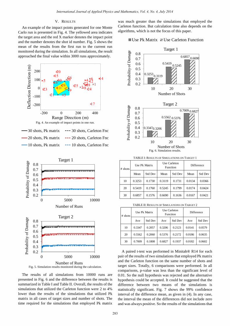
The results of all simulations from 10000 runs are

presented in Fig. 6 and the difference between the results is

summarized in Table I and Table II. Overall, the results of the

simulations that utilized the Carleton function were 2 to 4%

lower than the results of the simulations that utilized Pk

matrix in all cases of target sizes and number of shots. The

time required for the simulations that employed Pk matrix

was much greater than the simulations that employed the

Carleton function. But calculation time also depends on the

algorithms, which is not the focus of this paper.

0.3253

0.5419

0.6857

0.3119

0.5245

0.6690

0.2

0.3

0.4

0.5

0.6

0.7

0.8

10 20 30

Pro

bab

ilit

y o

f D

amag

e

Number of Shots

Target 1

Use Pk Matrix Use Carleton Function

0.3347

0.5562

0.7009

0.3206

0.5376

0.6827

0.2

0.3

0.4

0.5

0.6

0.7

0.8

10 20 30

Pro

bab

ilit

y o

f D

amag

e

Number of Shots

Target 2

Fig. 6. Simulation results.

TABLE I: RESULTS OF SIMULATIONS ON TARGET 1

Mean Std Dev Mean Std Dev Mean Std Dev

10 0.3253 0.1730 0.3119 0.1731 0.0134 0.0366

20 0.5419 0.1760 0.5245 0.1799 0.0174 0.0424

30 0.6857 0.1576 0.6690 0.1636 0.0167 0.0421

# shotsUse Pk Matrix

Use Carleton

FunctionDifference

TABLE II: RESULTS OF SIMULATIONS ON TARGET 2

Ave Std Dev Ave Std Dev Ave Std Dev

10 0.3347 0.2057 0.3206 0.2123 0.0141 0.0579

20 0.5562 0.2060 0.5376 0.2172 0.0186 0.0635

30 0.7009 0.1808 0.6827 0.1937 0.0182 0.0602

# shotsUse Pk Matrix

Use Carleton

FunctionDifference


283

An example of the impact points generated for one Monte

Carlo run is presented in Fig. 4. The yellowed area indicates

the target area and the red X marker denotes the impact point

and the number denotes the shot id number. Fig. 5 shows the

mean of the results from the first run to the current run

monitored during the simulation. In all simulations, the result

approached the final value within 3000 runs approximately.

A paired t-test was performed in Minitab® R14 for each

pair of the results of two simulations that employed Pk matrix

and the Carleton function on the same number of shots and

target sizes. Totally, 6 comparisons were performed. In all

comparisons, p-value was less than the significant level of

0.01. So the null hypothesis was rejected and the alternative

hypothesis could be accepted. It could be suggested that the

difference between two means of the simulations is

statistically significant. Fig. 7 shows the 99% confidence

interval of the difference mean, as given in (4). In any case,

the interval the mean of the differences did not include zero

and was always positive. So the results of the simulations that

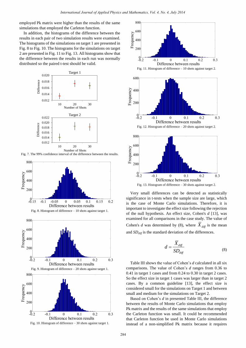
employed Pk matrix were higher than the results of the same

simulations that employed the Carleton function.

In addition, the histograms of the difference between the

results in each pair of two simulation results were examined.

The histograms of the simulations on target 1 are presented in

Fig. 8 to Fig. 10. The histograms for the simulations on target

2 are presented in Fig. 11 to Fig. 13. All histograms show that

the difference between the results in each run was normally

distributed so the paired t-test should be valid.

0.012

0.014

0.016

0.018

0.020

10 20 30

Dif

f ere

nce

Number of Shots

Target 1

0.012

0.014

0.016

0.018

0.020

0.022

10 20 30

Dif

fere

nce

Number of Shots

Target 2

Fig. 7. The 99% confidence interval of the difference between the results.

-0.15 -0.1 -0.05 0 0.05 0.1 0.15 0.20

200

400

600

800

Difference between results

Fre

quen

cy

Fig. 8. Histogram of difference – 10 shots against target 1.

-0.2 -0.1 0 0.1 0.2 0.30

200

400

600

800


Fre

quen

cy


-0.2 -0.1 0 0.1 0.2 0.30

200

400

600

800


Fre

quen

cy


-0.2 -0.1 0 0.1 0.2 0.30

200

400

600

800


Fre

quen

cy


-0.2 -0.1 0 0.1 0.2 0.30

200

400

600


Fre

quen

cy


-0.2 -0.1 0 0.1 0.2 0.30

200

400

600

800


Fre

quen

cy


Very small differences can be detected as statistically

significance in t-tests when the sample size are large, which

is the case of Monte Carlo simulations. Therefore, it is

important to investigate the effect size following the rejection

of the null hypothesis. An effect size, Cohen's d [13], was

examined for all comparisons in the case study. The value of

Cohen's d was determined by (8), where diffX is the mean

and SDdiff is the standard deviation of the differences.

diff

diff

SD

Xd

(8)

Table III shows the value of Cohen’s d calculated in all six

comparisons. The value of Cohen’s d ranges from 0.36 to

0.41 in target 1 cases and from 0.24 to 0.30 in target 2 cases.

So the effect size in target 1 cases was larger than in target 2

cases. By a common guideline [13], the effect size is

considered small for the simulations on Target 1 and between

small and medium for the simulations on Target 2.

Based on Cohen’s d in presented Table III, the difference

between the results of Monte Carlo simulations that employ

Pk matrix and the results of the same simulations that employ

the Carleton function was small. It could be recommended

that Carleton function be used in Monte Carlo simulations

instead of a non-simplified Pk matrix because it requires


284

coarser grid and less computing time, which is a critical

concern in a battlefield. However, users of the Carleton

function should be aware that small difference does exist.

VI. CONCLUSION

Two sets Monte Carlo simulations to determine the

probability of damage were performed in a case study of

multiple shots of unguided weapon against a uniform value

area target. The first set of the simulations utilized a Pk

matrix and the second set utilized the Carleton damage

function, of which parameters were determined based on a Pk

matrix. The simulations were performed for 10, 20, and 30

shots and 2 targets, of which the area is about 2.5 and 1.2

times of the weapon lethal area. Each simulation comprised

10000 runs. Both sets of simulations used the same impact

points that were randomly generated in accordance with the

weapon deliver accuracy. Totally, 6 paired t-tests were

carried out and there was statistically difference between the

simulation results that utilized the Pk matrix and the Carleton

function. Furthermore, the effect size was investigated and it

was suggested that the effect was small or almost medium in

all comparisons. So it could be recommended that the

Carleton be used in a simulation if the computing speed is

concerned.

ACKNOWLEDGMENT

The authors would like to thank Dr.Ganchai

Tanapornraweekit at Defence Technology Institute, Thailand,

for his advice on the lethality of fragmenting warheads and

Group Captain Chesda Kiriratnikom at Research and

Development Centre for Space and Aeronautical Science and

Technology, Royal Thai Air Force, for his suggestion on

weapon effectiveness analyses.

REFERENCES

[1] A. R. Eckle and S. A. Burr, “Mathematical models of target coverage

and missile allocation,” DTIC: AD-A953517, Military Operations

Research Society, USA, 1972.

[2] J. T. Klopcic, “A comparison of damage functions for use in artillery

effectiveness codes,” BRL-MR-3823, Ballistic Research Laboratory,

Aberdeen Proving Ground, MD, USA, 1990.

[3] J. S. Przemieniecki, Mathematical Methods in Defense Analyses, 3rd

ed., AIAA Education Series, USA, 2000.

[4] J. W. Kim, C. Lee, and B. R. Cho, “Using a Rayleigh-based circular

lethality coverage for naval surface fire support,” presented at

Industrial Engineering Research Conference, FL, USA, May 19-21,

2002.

[5] M. R. Driels, Weaponeering: Conventional Weapon System

Effectiveness, 2nd ed., AIAA Education Series, USA, 2013.

[6] C. M. Anderson, “Generalized weapon effectiveness modeling,”

Master’s Thesis, Naval Postgraduate School, Monterey, CA, USA,

2004.

[7] Joint Technical Coordinating Group for Munitions Effectiveness

Publications, AR 25-35/AFI 10-411/MCO 5600.43B/OPNAVINST

5600.23, 1996.

[8] N. Metropolis, “The beginning of the Monte Carlo method,” Los

Alamos Science, issue 15, pp. 125–130, 1987.

[9] R. E. Roger, “Stan Ulam, John von Neumann, and the Monte Carlo

method,” Los Alamos Science, issue 15, pp. 131–137, 1987.

[10] M. R. Driels and Y. S. Shin, “Determining the number of iterations for

Monte Carlo simulation of weapon effectiveness,” Technical Report,

Naval Postgraduate School, Monterey, CA, USA, 2004.

[11] R. Y. Rubinstein and D. P. Kroese, Simulation and the Monte Carlo

Method, 2nd ed., John Wiley and Sons, USA, 2008.

[12] A. Black, J. F. Mahoney, and B. D. Sivazlian, “Estimation of the

weapons parameters and their variances in the Carleton damage

function,” Variability of Measures of Weapons Effectiveness, vol. 6,

AFATL-TR-84-92, Air Force Armament Laboratory, USA, 1985.

[13] J. Cohen, Statistical Power Analysis for the Behavioral Sciences, 2nd

ed., Lawrence Erlbaum Associates, USA, 1988.

Pawat Chusilp received his B.S. in mechanical

engineering from Chulalongkorn University, Thailand

in 1999, M.S. and Ph.D. in mechanical engineering

from University of Southern California, USA in 2001

and 2004 respectively. He joined Defence Technology

Institute, Thailand in 2009 and is currently a researcher

in aeronautical engineering laboratory. His research

interests are in aerodynamics, trajectory simulations,

and target coverage.

Weerawut Charubhun earned his B.S. in mechanical

engineering from Kasetsart University, Thailand in

1999 and M.S. in mechanical engineering from

University of Sydney, Australia in 2002. He joined

Defence Technology Institute, Thailand in 2009 and is

currently a researcher in aeronautical engineering

laboratory. His research interests are in aerodynamics,

computational fluid dynamics, and trajectory

simulations.

Pattadon Koanantachai received his B.S. in

aerospace engineering and M.S. in mechanical

engineering from King Mongkut’s University of

Technology North Bangkok, Thailand in 2010 and

2014 respectively. He joined Defence Technology

Institute, Thailand in 2014 and has been working as a

researcher in aeronautical engineering laboratory. His

research interests are in aircraft designs, computational

fluid dynamics, and composite airframe structures.


285

TABLE III: COHEN’S D VALUES

# Shots Target 1 Target 2

10 0.367 0.243

20 0.410 0.293

30 0.396 0.303

Documents

Monte Carlo Simulations of Weapon Effectiveness …€”Carleton damage function has been commonly ... multiple shots of an unguided artillery weapon against an area target was chosen