Monte Carlo Sampling-Based Methods for Stochastic Optimization

Tito Homem-de-Mello

School of Business

Universidad Adolfo Ibanez

Santiago, Chile

tito.hmello@uai.cl

Guzin Bayraksan

Integrated Systems Engineering

The Ohio State University

Columbus, Ohio

bayraksan.1@osu.edu

January 22, 2014

Abstract

This paper surveys the use of Monte Carlo sampling-based methods for stochastic optimization

problems. Such methods are required when—as it often happens in practice—the model involves

quantities such as expectations and probabilities that cannot be evaluated exactly. While estimation

procedures via sampling are well studied in statistics, the use of such methods in an optimization

context creates new challenges such as ensuring convergence of optimal solutions and optimal val-

ues, testing optimality conditions, choosing appropriate sample sizes to balance the effort between

optimization and estimation, and many other issues. Much work has been done in the literature

to address these questions. The purpose of this paper is to give an overview of some of that work,

with the goal of introducing the topic to students and researchers and providing a practical guide

for someone who needs to solve a stochastic optimization problem with sampling.

1 Introduction

Uncertainty is present in many aspects of decision making. Critical data, such as future demands

for a product or future interest rates, may not be available at the time a decision must be made.

Unexpected events such as machine failures or disasters may occur, and a robust planning process

must take such possibilities into account. Uncertainty may also arise due to variability in data, as

it happens for example in situations involving travel times on highways. Variability also produces

uncertainty in physical and engineering systems, in which case the goal becomes, for example, to

provide a reliable design. Such problems fall into the realm of stochastic optimization, an area that

comprises modeling and methodology for optimizing the performance of systems while taking the

uncertainty explicitly into account.

1

A somewhat generic formulation of a stochastic optimization problem has the form

minx∈X{g0(x) := E[G0(x, ξ)] | E[Gk(x, ξ)] ≤ 0, k = 1, 2, . . . ,K} , (SP)

where Gk, k = 0, 1, . . . ,K are extended real-valued functions with inputs being the decision vector

x and a random vector ξ. We use K = 0 to denote (SP) with only deterministic constraints.

Typically, there are finitely many stochastic constraints (K <∞) but this does not need to be the

case. In fact, there can be uncountably many stochastic constraints (see Section 6.3). The set of

deterministic constraints x must satisfy is denoted by X ⊂ Rdx and Ξ ⊂ Rdξ denotes the support

of ξ, where dx and dξ are the dimensions of the vectors x and ξ, respectively. We assume that ξ

has a known distribution, P , that is independent of x, and the expectations in (SP), taken with

respect to the distribution of ξ, are well-defined and finite for all x ∈ X.

A wide variety of problems can be cast as (SP) depending on K, X and Gk, k = 0, 1, 2, . . . ,K.

For example, in a two-stage stochastic linear program with recourse, K = 0, X = {Ax = b, x ≥ 0},and G0(x, ξ) = cx+ h(x, ξ), where h(x, ξ) is the optimal value of the linear program

h(x, ξ) = miny

qy

s.t. Wy = r − T x, y ≥ 0.

Here, ξ is a random vector that is comprised of random elements of q, W , R and T .

In contrast, in a stochastic program with a single probabilistic constraint (i.e., P (A′x ≥ b′) ≤ α),

we have K = 1, G0(x, ξ) = cx and

G1(x, ξ) = I{A′x ≥ b′} − α,

where I{E} denotes the indicator function that takes value 1 if the event E happens and 0 otherwise

and α ∈ (0, 1) is a desired probability level. In this case, ξ is comprised of random elements of A′

and b′. Here, the decision maker requires that the relationship A′x ≥ b be satisfied with probability

no more than α.

Several other variants of (SP) exist; for example, the objective function may be expressed not

as a classical expectation but in a different form, such as a value-at-risk or conditional value-at-

risk involving the random variable G0(x, ξ) or multiple stages can be considered (see e.g., Section

3.2 for multistage stochastic linear programs). There are also cases where the distribution of the

underlying random vector ξ depends on the decision variables x even if such dependence is not

known explicitly; we shall discuss some of these variations later. For now, we assume that (SP) is

the problem of interest, and that K = 0 in (SP) so that we only have X, the set of deterministic

constraints in (SP)—the case of stochastic constraints is dealt with in Section 6. To simplify

notation, we will drop the index 0 from the objective function in (SP). We will refer to (SP) as

the “true” optimization problem (as opposed to the approximating problems to be discussed in the

sequel).

2

Benefiting from advances in computational power as well as from new theoretical developments,

the area of stochastic optimization has evolved considerably in the past few years, with many recent

applications in areas such as energy planning, national security, supply chain management, health

care, finance, transportation, revenue management, and many others. New applications bring new

challenges, particularly concerning the introduction of more random variables to make the models

more realistic. In such situations, it is clearly impossible to enumerate all the possible outcomes,

which precludes the computation of the expectations in (SP). As a very simple example, consider

a model with dξ independent random variables, each with only two possible alternatives; the total

number of scenarios is thus 2dξ , and so even for moderate values of dξ it becomes impractical to

take all possible outcomes into account. In such cases, sampling techniques are a natural tool to

use.

Sampling-based methods have been successfully used in many different applications of stochastic

optimization. Examples of such applications can be found in vehicle routing (Kenyon and Morton

[128], Verweij et al. [236]), engineering design (Royset and Polak [206]), supply chain network design

(Santoso et al. [213]), power generation and transmission (Jirutitijaroen and Singh [122]), and asset

liability management (Hilli et al. [104]), among others. More recently, Byrd et al. [34] used these

techniques in the context of machine learning. The appeal of sampling-based methods results from

the fact that they often approximate well, with a small number of samples, problems that have a

very large number of scenarios; see, for instance, Linderoth et al. [152] for numerical reports.

There are multiple ways to use sampling methods in problem (SP). A generic way of describing

them is to construct an approximating problem as follows. Consider a family {gN (·)} of random

approximations of the function g(·), each gN (·) being defined as

gN (x) :=1

N

N∑j=1

G(x, ξj), (1)

where {ξ1, . . . , ξN} is a sample from the distribution1 of ξ. When ξ1, . . . , ξN are mutually inde-

pendent, the quantity gN (x) is called a (standard or crude) Monte Carlo estimator of g(x). Given

the family of estimators {gN (·)} defined in (1), one can construct the corresponding approximating

program

minx∈X

gN (x). (2)

Note that for each x ∈ X the quantity gN (x) is random variable, since it depends on the sample

{ξ1, . . . , ξN}. So, the optimal solution(s) and the optimal value of (2) are random as well. Given

a particular realization {ξ1, . . . , ξN} of the sample, we define

gN (x, ξ1, . . . , ξN ) :=1

N

N∑j=1

G(x, ξj). (3)

1Throughout this paper, we will use the terminology “sample [of size N ] from the distribution of ξ” to indicate aset of N random variables with the same distribution as ξ. Also, recall that we drop the subscript 0 from g and Gas we assume here that K = 0.

3

A remark about the notation is in order. In (3), we write explicitly the dependence on ξ1, . . . , ξN to

emphasize that, given x, gN (x, ξ1, . . . , ξN ) is a number that depends on a particular realization of the

sample. Such notation also helps, in our view, to understand the convergence results in Section 2. In

contrast, in (1) we do not write it in that fashion since gN (x) is viewed as a random variable. While

such a distinction is usually not made in the literature, we adopt it here for explanatory purposes

and to emphasize that the problem minx∈X gN (x, ξ1, . . . , ξN ) is a deterministic one. Later in the

paper we will revert to the classical notation and write simply gN (x), with its interpretation as a

number or a random variable being understood from the context. Also, throughout the majority

of the paper we assume that realizations are generated using the standard Monte Carlo method,

unless otherwise stated. We discuss alternative sampling methods in Section 7.

Consider now the following algorithm:

ALGORITHM 1

1. Choose an initial solution x0; let k := 1.

2. Obtain a realization {ξk,1, . . . , ξk,Nk} of {ξ1, . . . , ξNk}.

3. Perform some optimization steps on the function gNk(·, ξk,1, . . . , ξk,Nk) (perhaps using infor-

mation from previous iterations) to obtain xk.

4. Check some stopping criteria; if not satisfied, set k := k + 1 and go back to Step 2.

Note that although we call it an “algorithm”, Algorithm 1 should be understood as a generic frame-

work that allows for many variations based on what is understood by “perform some optimization

steps,” “check some stopping criterion,” and the choice of the sample size Nk. For example, con-

sider the Sample Average Approximation (SAA) approach, which has appeared in the literature

under other names as well, as discussed in Section 2. In such an approach, by solving the problem

minx∈X

gN (x, ξ1, . . . , ξN ) (4)

—which is now completely deterministic (since the realization is fixed), so it can be solved by stan-

dard deterministic optimization methods—we obtain specific estimates of the optimal solution(s)

and the optimal value of (SP). The SAA approach can be viewed as a particular case of Algorithm 1

whereby Step 3 fully minimizes the function gN (·, ξ1,1, . . . , ξ1,N1), so Algorithm 1 stops after one

(outer) iteration. We will discuss the SAA approach and its convergence properties in Section 2.

As another example, consider the classical version of the Stochastic Approximation (SA) method,

which is defined by the recursive sequence

xk+1 := xk − αkηk, k ≥ 0,

where ηk is a random direction—usually an estimator of the gradient ∇g(xk), such as ∇G(xk, ξ)—

and αk is the step-size at iteration k. Clearly, the classical SA method falls into the general

4

framework of Algorithm 1 where Nk = 1 for all k and Step 3 consists of one optimization step

(xk+1 := xk − αkηk). We will discuss the SA method and some of its recent variants later.

As the above discussion indicates, many questions arise when implementing some variation of

Algorithm 1, such as:

• What sample size Nk to use at each iteration?

• Should a new realization of {ξ1, . . . , ξNk} be drawn in Step 2, or can one extend the realization

from the previous iteration?

• How should this sample be generated to begin with? Should one use crude Monte Carlo or

can other methods—for instance, aimed to reduce variability—be used?

• How to perform an optimization step in Step 3 and how many steps should be taken?

• How to design the stopping criteria in Step 4 in the presence of sampling-based estimators?

• What can be said about the quality of the solution returned by the algorithm?

• What kind of asymptotic properties does the resulting algorithm have?

Much work has been done in the literature to address these questions. The purpose of this paper

is to give an overview of some of that work, with the goal of providing a practical guide for someone

who needs to solve a stochastic optimization problem with sampling. In that sense, our mission

contrasts starkly with that of the compilations in Shapiro [218] and Shapiro et al. [227, Chapter 5],

which provide a comprehensive review of theoretical properties of sampling-based approaches for

problem (SP). Our work also complements the recent review by Kim et al. [131], who focus on a

comparative study of rates of convergence.

We must emphasize, though, that our goal is not to describe in detail specific algorithms

proposed in the literature for some classes of stochastic optimization problems. Such a task would

require far more space than what is reasonable for a review paper, and even then we probably

would not do justice to the subtleties of some of the algorithms. Instead, we refer the reader to the

appropriate references where such details can be found.

It is interesting to notice that problem (SP) has been studied somewhat independently by two

different communities, who view the problem from different perspectives. On one side is the opti-

mization community, who wants to solve “mathematical programming problems with uncertainty,”

which means that typically the function g(·) has some structure such as convexity, continuity, dif-

ferentiability, etc., that can be exploited when deciding on a particular variation of Algorithm 1.

On the other side is the simulation community, who focuses on methods that typically do not

make any assumptions about the structure of g, and the approximation g(x) is viewed as the re-

sponse of a “black box” to a given input x. The goal then becomes to cleverly choose the design

points x—often via some form of random search—in order to find a solution that has some desir-

able properties such as asymptotic optimality or probabilistic guarantees of being a good solution.

5

The resulting algorithms are often called simulation optimization methods. Reviews of simulation

optimization—sometimes called optimization via simulation—within the past decade can be found

in Fu [82], Andradottir [5] and Chen et al. [43], although much has been done since the publication

of those articles.

There are, of course, many common elements between the problems and methods studied by

the optimization and the simulation communities, which has been recognized in books that “bridge

the gap” such as Rubinstein and Shapiro [210] and Pflug [190]. In fact, the line between simulation

optimization and mathematical programs under uncertainty has become increasingly blurry in

recent years, as illustrated by the recent book by Powell and Ryzhov [198]. While we acknowledge

that the present survey does not fully connect these two areas—it is certainly more focused on the

mathematical programming side—we hope that this article will help to bring awareness of some

techniques and results to both communities.

We conclude these introductory remarks with a cautionary note. Writing a review of this kind,

where the literature is scattered among optimization, simulation, and statistics journals, inevitably

leads to omissions despite our best efforts. Our apologies to those authors whose works we have

failed to acknowledge in these pages.

The remainder of this paper is organized as follows. In Section 2 we discuss some theoretical

properties of the SAA approach and illustrate them by applying the technique to the classical

newsvendor problem. Section 3 discusses approaches based on sequential sampling whereby new

samples are drawn periodically—as opposed to SAA where a fixed sample is used throughout the

algorithm. The practical issue of evaluating the quality of a given solution—which is intrinsically

related to testing stopping criteria for the algorithms—is studied in Section 4. Another important

topic for practical implementation of sampling-based methods is the choice of appropriate sample

sizes; that issue is discussed in Section 5. In Section 6 we study the case of problems with stochastic

constraints, which as we will see require special treatment. Monte Carlo methods are often enhanced

by the use of variance reduction techniques; the use of such methods in the context of sampling-

based stochastic optimization is reviewed in Section 7. There are of course many topics that are

relevant to the subject of this survey but which we cannot cover due to time and space limitations;

we briefly discuss some of these topics in Section 8. Finally, we present some concluding remarks

and directions for future research in Section 9.

2 The SAA approach

We consider initially the SAA approach, which, as discussed earlier, consists of solving problem (4)

using a deterministic algorithm. This idea has appeared in the literature under different names: in

Robinson [202], Plambeck et al. [195] and Gurkan et al. [95] it is called the sample-path optimization

method, whereas in Rubinstein and Shapiro [210] it is called the stochastic counterpart method. The

term “sample average approximation” appears to have been coined by Kleywegt et al. [134]. It is

important to note that SAA itself is not an algorithm; the term refers to the approach of replacing

6

the original problem (SP) with its sampling approximation, which is also sometimes called the

external sampling approach in the literature.

The analysis of SAA typically assumes that the approximating problem is solved exactly, and

studies the convergence of the estimators of optimal solutions and of optimal values obtained from

(2) in that context. This type of analysis has appeared in the literature pre-dating the papers

mentioned above, without a particular name for the approach—see, for instance, Dupacova and

Wets [70], King and Rockafellar [133] and Shapiro [216, 217].

We discuss now the ideas behind the main convergence results. Our goal here is to illustrate the

results rather than provide detailed mathematical statements—for that, we refer to the compilations

in Shapiro [218] and Shapiro et al. [227, Chapter 5] and papers therein. To illustrate the convergence

results to be reviewed in the sequel, we shall study the simple example of the classical newsvendor

problem. Of course, such a problem can be solved exactly and hence there is no need to use a

sampling method; however, this is precisely the reason why we use that problem in our examples,

so we can compare the approximating solutions with the exact ones in order to illustrate convergence

results. Moreover, the unidimensionality of that model will allow us to depict some of the results

graphically. Let us begin with a definition.

Example 1. (Newsvendor Problem). Consider a seller that must choose the amount x of inventory

to obtain at the beginning of a selling season. The decision is made only once—there is no oppor-

tunity to replenish inventory during the selling season. The demand ξ during the selling season

is a nonnegative random variable with cumulative distribution function F . The cost of obtaining

inventory is c per unit. The product is sold at a given price r per unit during the selling season,

and at the end of the season unsold inventory has a salvage value of v per unit. The seller wants

to choose the amount x of inventory that solves

minx{g(x) = E [cx− rmin{x, ξ} − vmax{x− ξ, 0}]} . (5)

It is well known that, if v < c < r, then any x∗ that satisfies

F (x) ≤ r − cr − v

for all x < x∗ and F (x) ≥ r − cr − v

for all x > x∗

is an optimal amount of inventory to obtain at the beginning of the selling season. That is, the set

of optimal solutions is given by the set of γ-quantiles of the distribution of ξ, which can be written

as

S := {z ∈ R : P (ξ ≥ z) ≥ 1− γ and P (ξ ≤ z) ≥ γ} , (6)

where γ = (r − c)/(r − v). Note that S is a nonempty closed interval for all γ ∈ (0, 1).

We will be referring back to the newsvendor problem often throughout the remainder of this

section. Let us now apply the SAA approach to this problem.

Example 2. (Application of the SAA Approach to the Newsvendor Problem). The approximation

7

of problem (5) is written as

minx

{gN (x, ξ1, . . . , ξN ) :=

1

N

N∑i=1

[cx− rmin{x, ξi} − vmax{x− ξi, 0}

]}. (7)

Any sample γ-quantile is an optimal solution to the above problem. For example, we can take

xN = ξ(dγNe) as an optimal solution, where ξ(1), . . . , ξ(N) represent an ordering of the realizations

(in ascending order) and dae is the smallest integer larger than or equal to a.

2.1 Consistency

We start by defining some notation. Let xN and SN denote respectively an optimal solution and

the set of optimal solutions of (2). Moreover, let νN denote the optimal value of (2). Then, xN ,

SN and νN are statistical estimators of an optimal solution x∗, the set of optimal solutions S∗ and

the optimal value ν∗ of the true problem (SP), respectively.

The first issue to be addressed is whether these estimators are (strongly) consistent, i.e. whether

they converge to the respective estimated values with probability one. It is important to understand

well what such a statement means: given a realization {ξ1, ξ2, . . . , } of {ξ1, ξ2, . . . , }, let xN be an

optimal solution and νN the optimal value2 of problem (4) defined with the first N terms of the

sequence {ξ1, ξ2, . . . , }. Consistency results make statements about convergence of the sequences

{xN} and {νN}. If such statements hold regardless of the realization {ξ1, ξ2, . . . , } (except perhaps

for some realizations on a set of probability zero), then we have convergence “with probability

one” (w.p.1), or “almost surely” (a.s.). When dealing with convergence of solutions, it will be

convenient to use the notation dist(x,A) to denote the distance from a point x to a set A, defined

as infa∈A ‖x− a‖.To illustrate the consistency of the SAA estimators, we will next use specific instances of the

newsvendor problem. The first newsvendor instance has demand modeled as an exponential random

variable and it has a unique optimal solution. Later, we will look at another instance with a discrete

uniform demand, which has multiple optimal solutions. The two instances have the same parameters

otherwise. The results of the SAA approach to these instances are shown in Table 1 and Figures

1–4.

Example 3. (Newsvendor Instance with Exponential Demand). Consider the newsvendor problem

defined in Example 1 with model parameters r = 6, c = 5, v = 1 and demand that has Exponen-

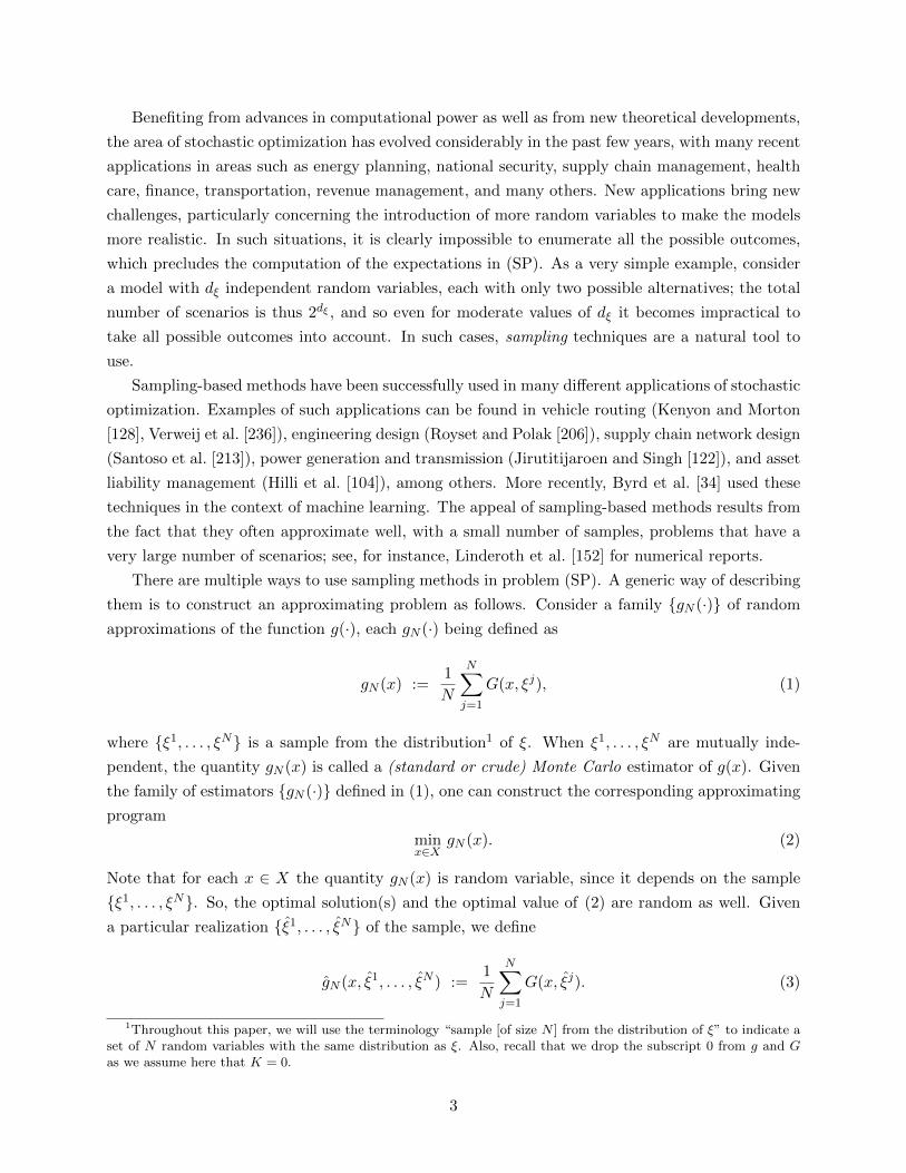
tial(10) distribution (i.e., the mean is 10). Figure 1a depicts the objective function g(·) for this

instance as well as the approximations gN (·, ξ1, . . . , ξN ) for a particular realization {ξ1, ξ2, . . . , }with various values of N = 10, 30, 90, 270. Table 1a shows the optimal solutions and optimal values

for the same functions. We see that, for this realization, N = 270 approximates the true function

very closely and the quality of the other approximations depends on the tolerance allowed.

2To be precise, we should write xN and νN as functions of the realization {ξ1, ξ2, . . . , }, but we omit that for thesake of brevity of notation.

8

0 0.5 1 1.5 2 2.5 3 3.5 4 4.5 5−1.5

−1

−0.5

0

0.5

1

1.5

2

2.5

3

x

g N(x

)

true functionN=10N=30N=90N=270

(a) Exponential demand

0 0.5 1 1.5 2 2.5 3 3.5 4 4.5 5−2.5

−2

−1.5

−1

−0.5

0

0.5

1

1.5

2

x

g N(x

)

true functionN=10N=30N=90N=270

(b) Discrete uniform demand

Figure 1: Newsvendor function and corresponding sample average approximations.

N 10 30 90 270 ∞xN 1.46 1.44 1.54 2.02 2.23νN -1.11 -0.84 -0.98 -1.06 -1.07

(a) Exponential demand

N 10 30 90 270 ∞xN 2 3 3 2 [2,3]νN -2.00 -2.50 -1.67 -1.35 -1.50

(b) Discrete uniform demand

Table 1: Optimal solution and optimal values for the newsvendor function; the column ∞ refers tothe true function.

The above example suggests that we have νN → ν∗ and xN → x∗. How general is that

conclusion? It is clear that convergence of xN and νN to their estimated values cannot be expected

if gN (x) defined in (2) does not converge to g(x) for some feasible point x ∈ X. However, just having

pointwise convergence of gN (x) to g(x) (w.p.1) for all x ∈ X is not enough; stronger conditions

are required. A sufficient condition that can often be verified in practice is that gN (·) converge

uniformly to g(·) on X w.p.1, i.e., for (almost) any realization {ξ1, ξ2, . . . , }, given ε > 0 there

exists N0 such that

|gN (x, ξ1, . . . , ξN )− g(x)| < ε for any N ≥ N0 and all x ∈ X.

Notice that in the above definition the value of N0 depends on the realization {ξ1, ξ2, . . . , }. In

other words, the accuracy of the approximation for a given N depends on the realization. The

uniform convergence condition is satisfied in many cases found in practice—for example, when the

function G(x, ξ) is convex and continuous in x for almost all ξ and X is a compact, convex set.

Under the uniform convergence assumption, we have the following results:

1. νN → ν∗ w.p.1,

2. Under additional assumptions involving boundedness of S∗ and continuity of the objective

function, dist(xN , S∗)→ 0 w.p.1.

Note that item 2 above does not ensure that the estimators xN converge w.p.1; rather, it says

9

that xN gets increasingly closer to the set S∗ as N gets large. Of course, in case there is a unique

optimal solution x∗—as it was the case in the newsvendor instance with Exponential demand shown

in Figure 1a—then xN converges to x∗ w.p.1. To illustrate a situation where xN might not converge,

consider another instance of the newsvendor problem.

Example 4. (Newsvendor Instance with Discrete Uniform Demand). Consider a newsvendor

problem with the same parameters as in Example 3 but with demand having discrete uniform dis-

tribution on {1, 2, . . . , 10}. Figure 1b depicts the functions g(·) and gN (·, ξ1, . . . , ξN ) for a particular

realization for each of the sample sizes N = 10, 30, 90, 270. The corresponding optimal solutions

and optimal values are shown in Table 1b. Here the optimal solution set S∗ is the interval [2, 3]. We

see that, while the optimal values νN converge to ν∗, the solutions xN alternate between 2 and 3.

It is interesting to observe, however, that xN is actually inside the optimal set S∗ for all N depicted

in the figure even when the approximation is poor (as in the case of N = 30). In other words, not

only dist(xN , S∗)→ 0 as predicted by the theory but in fact dist(xN , S

∗) = 0 for sufficiently large

N . This situation is typical of a class of problems with discrete distributions with a finite number

of realizations, as we shall see later.

Figures 1a and 1b have illustrated the behavior of the approximation for a single realization of

the random variables for a variety of sample sizes N . But how typical are those realizations?

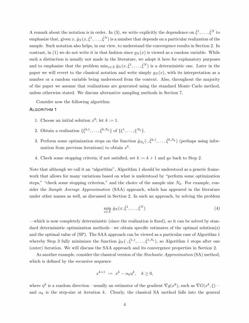
Example 5. (1,000 SAAs on the Newsvendor Instances). Figures 2a and 2b depict the behavior

of the approximations for 1,000 realizations for a fixed sample size N = 270 for the cases of both

exponential and discrete uniform demand studied above. Two observations can be made from the

figures. First, as mentioned earlier, the quality of the approximation depends on the realization—as

we can see in the figures, some of the approximations are very close to the true function whereas

others are far off. Second, many of the approximations lie below the true function, therefore yielding

an estimate νN ≤ ν∗, whereas in other cases νN ≥ ν∗.

0 0.5 1 1.5 2 2.5 3 3.5 4 4.5 5−2

−1.5

−1

−0.5

0

0.5

1

1.5

2

2.5

x

g N(x

)

(a) Exponential demand

0 0.5 1 1.5 2 2.5 3 3.5 4 4.5 5−2.5

−2

−1.5

−1

−0.5

0

0.5

1

1.5

2

x

g N(x

)

(b) Discrete uniform demand

Figure 2: 1,000 replications of SAA approach to newsvendor function with N = 270.

Given the results of Example 5, it is natural then to consider what happens on the average.

10

Consider for the moment the case where N = 1. Then, we have

E [ν1] = E[minx∈X

G(x, ξ)

]≤ min

x∈XE [G(x, ξ)] = min

x∈Xg(x) = ν∗,

where the inequality follows from the same principle that dictates that the sum of the minima of

two sequences is less than or equal to the the minimum of the sum of the two sequences. It is easy

to generalize the above inequality for arbitrary N , from which we conclude that

E [νN ] ≤ ν∗. (8)

That is, on the average, the approximating problem yields an optimal value that is below or at most

equal to ν∗. In statistical terms, νN is a biased estimator of ν∗. It is possible to show, however,

that the bias ν∗−E [νN ] decreases monotonically in N and goes to zero as N goes to infinity (Mak

et al. [158]).

We conclude this subsection with the observation that in the above discussion about convergence

of optimal solutions it is important to emphasize that by “optimal solution” we mean a global

optimal solution. While this is not an issue in case of convex problems, it becomes critical in

case of nonconvex functions. For example, Bastin et al. [15] present a simple example where a

local minimizer of the approximating problem converges to a point which is neither a local nor a

global minimizer of the original problem. In such cases it is important to look at convergence of

second-order conditions. We refer to that paper for a detailed discussion.

2.2 Rates of convergence

In the discussion above we saw how, under appropriate conditions, we expect the approximating

problem (2) to yield estimators xN and νN that approach their true counterparts w.p.1 as N goes

to infinity. A natural question that arises is how large N must be in order to yield “good enough”

estimates. Such a question can be framed in terms of rates of convergence, which we study next.

Convergence of optimal values

We first discuss the rate of convergence of the optimal value estimators νN . To understand the

main results—which we shall describe soon—let us consider again the newsvendor example with

the same parameters used earlier, for exponentially distributed demand.

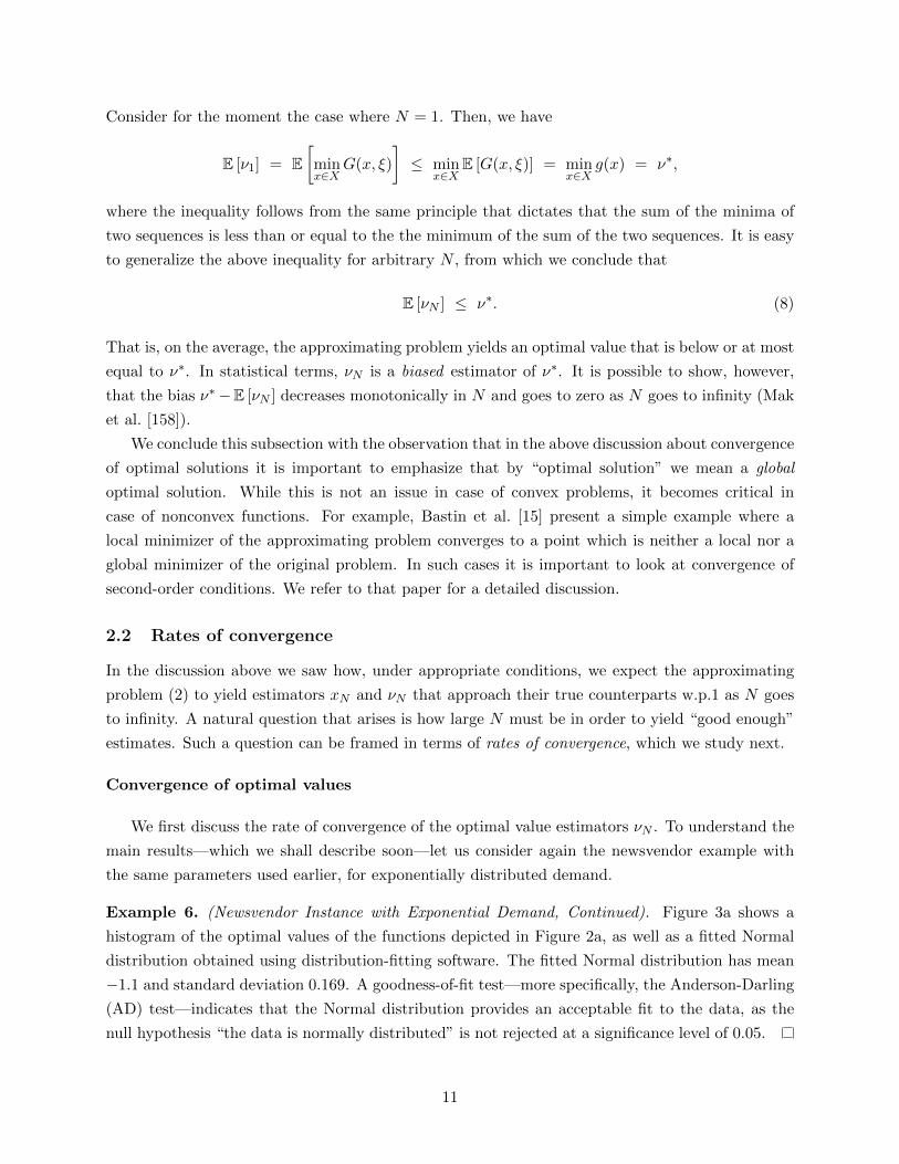
Example 6. (Newsvendor Instance with Exponential Demand, Continued). Figure 3a shows a

histogram of the optimal values of the functions depicted in Figure 2a, as well as a fitted Normal

distribution obtained using distribution-fitting software. The fitted Normal distribution has mean

−1.1 and standard deviation 0.169. A goodness-of-fit test—more specifically, the Anderson-Darling

(AD) test—indicates that the Normal distribution provides an acceptable fit to the data, as the

null hypothesis “the data is normally distributed” is not rejected at a significance level of 0.05.

11

Probability density function

Histogram Normal

v-0,8-1-1,2-1,4-1,6-1,8

f(v)

0,28

0,26

0,24

0,22

0,2

0,18

0,16

0,14

0,12

0,1

0,08

0,06

0,04

0,02

0

(a) Exponential demand

Probability density function

Histogram Normal

v-1,2-1,4-1,6-1,8-2

f(v)

0,3

0,28

0,26

0,24

0,22

0,2

0,18

0,16

0,14

0,12

0,1

0,08

0,06

0,04

0,02

0

(b) Discrete uniform demand

Figure 3: Histogram of optimal values of SAA approach to newsvendor function with N = 270.

To view that result of Example 6 in a more general context, consider a fixed x ∈ X. Then,

under mild assumptions ensuring finiteness of variance, the Central Limit Theorem tells us that

√N [gN (x)− g(x)]

d→ Y (x) ∼ Normal(0, σ2(x)), (9)

where σ2(x) := Var[G(x, ξ)], the notationd→ indicates convergence in distribution to a random

variable Y (x) and the symbol ∼ indicates that Y (x) has Normal(0, σ2(x)) distribution. That is,

for large N the random variable gN (x) is approximately normally distributed with mean g(x) and

variance σ2(x)/N . As it turns out, such a property still holds when gN (x) and g(x) in (9) are

replaced by their minimum values over X. More precisely, under assumptions of compactness

of X and Lipschitz continuity of the function G(·, ξ)—which, roughly speaking, means that the

derivatives of G(·, ξ) are bounded by a constant, so G(·, ξ) does not vary wildly—we have that

√N(νN − ν∗)

d→ infx∈S∗

Y (x). (10)

Note that the expression on the right-hand side of (10) indicates a random variable defined as

the minimum (or infimum) of normally distributed random variables. In general, the resulting

distribution is not Normal; however, when the original problem has a unique solution x∗, then

S∗ = {x∗} and in that case the right hand side in (10) is indeed normally distributed with mean

zero and variance σ2(x∗). Let us take a closer look at Example 6.

Example 7. (Newsvendor Instance with Exponential Demand, Continued). As seen earlier, this

instance of the newsvendor problem has a unique optimal solution, which explains the nice behavior

of νN shown in Figure 3a. In fact, recall from Table 1a that the optimal value corresponding to

the optimal solution x∗ = 2.23 is ν∗ = −1.07. Moreover, the variance of the expression inside

the integral in (5) at the optimal solution x∗ = 2.23 can be estimated (using a very large sample

size) as σ2(x∗) ' 7.44; therefore, the theory predicts that, for large N , the estimator νN has

12

approximately Normal(ν∗,σ2(x∗)/N) =Normal(−1.07, 7.44/N) distribution. With N = 270, the

standard deviation is√

7.44/270 = 0.166, so we see that this asymptotic distribution very much

agrees with the Normal distribution that fits the histogram in Figure 3a.

The situation is different in the case of multiple optimal solutions. As mentioned, we do not

expect νN to be normally distributed, since the limit distribution is given by the infimum of

Normal distributions over the set of optimal solutions (recall equation (10)). This is the case in

the newsvendor instance with discrete uniform distribution (S∗ = [2, 3]).

Example 8. (Newsvendor Instance with Discrete Uniform Demand, Continued). Figure 3b shows

a histogram of the optimal values of the functions depicted in Figure 2b. Although the histogram

may seem to be reasonably close to a Normal distribution, that distribution does not pass the AD

goodness-of-fit test even at a significance level of 0.01.

The convergence result (10) leads to some important conclusions about the rate of convergence

of the bias ν∗ − E [νN ] to zero. Indeed, suppose for the sake of this argument that convergence

in distribution implies convergence of expectations (which holds, for example, when a condition

such as uniform integrability is satisfied). Then, it follows from (10) that√N(E[νN ] − ν∗) →

E[infx∈S∗ Y (x)]. Recall from (9) that each Y (x) has mean zero. Then, E [infx∈S∗ Y (x)] is less than

or equal to zero and it is often strictly negative when S∗ has more than one element. Thus, when

that happens, the bias E[νN ] − ν∗ is exactly of order N−1/2, i.e., it cannot go to zero faster than

N−1/2. On the other hand, when S∗ has a unique element, we have√N(E[νN ]− ν∗)→ 0, i.e., the

bias goes to zero faster than N−1/2. For example, Freimer et al. [79] compute the exact bias for the

newsvendor problem when demand has uniform distribution on (0,1)—in which case the optimal

solution x∗ = γ is unique—as

E[νN ]− ν∗ =γ(1− γ)

2(N + 1),

so we see that in this case the bias is of order N−1. In general, the rate of convergence of bias for a

stochastic program can take a variety of values N−p for p ∈ [1/2,∞); see, for instance, Example 5

in Bayraksan and Morton [20].

Convergence of optimal solutions

It is possible to study the rate of convergence of optimal solutions as well. The convergence

properties of optimal solutions depend on the smoothness of the objective function for a class of

problems. Let us take a closer look at the two newsvendor instances to gain an understanding.

Example 9. (Optimal Solutions of the SAAs of the Newsvendor Instances). Notice that the

objective function of the exponential demand instance is smooth. We can see in Figure 1a and

Table 1a the estimate xN approaches the optimal solution x∗. In contrast, the results of the discrete

uniform demand instance—which has a nonsmooth objective function—depicted in Figure 1b and

Table 1b show that the estimate xN coincides with one of the optimal solutions in S∗. Typically

this happens once N large enough but xN can be far away if N is small.

13

Let us discuss initially the smooth case. As before, we first illustrate the ideas with the newsven-

dor problem.

Example 10. (Newsvendor Instance with Exponential Demand, Continued). Figure 4a shows a

histogram of the optimal solutions of the functions depicted in Figure 2a, as well as a fitted Normal

distribution, which passes the AD goodness-of-fit test at a significance level of 0.15. The fitted

Normal distribution has mean 2.24 (recall that x∗ = 2.23) and standard deviation 0.308.

Probability density function

Histogram Normal

x32,521,5

f(x)

0,28

0,26

0,24

0,22

0,2

0,18

0,16

0,14

0,12

0,1

0,08

0,06

0,04

0,02

0

(a) Exponential demand

Probability mass function

Sample

x32

f(x)

0,56

0,52

0,48

0,44

0,4

0,36

0,32

0,28

0,24

0,2

0,16

0,12

0,08

0,04

0

(b) Discrete uniform demand

Figure 4: Histogram of optimal solutions of SAA approach to newsvendor function with N = 270.

Example 10 suggests that the estimator xN is approximately normally distributed for large

N . In a more general context, of course, xN is a vector, so we can conjecture whether xN has

approximately multivariate Normal distribution for large N . Indeed, suppose that there is a unique

solution x∗ and suppose that the function g(x) is twice differentiable at x0. Suppose for the moment

that the problem is unconstrained, i.e., X = Rn. Then, under mild additional conditions, we have

√N(xN − x∗)

d→ Normal(0, H−1ΨH−1), (11)

where H = ∇2xxg(x∗), and Ψ is the asymptotic covariance matrix of

√N [∇gN (x∗) −∇g(x∗)]. So,

we see that when N is sufficiently large the estimator xN has approximately multivariate Normal

distribution. For details on this result, as well as an extension to the constrained case, we refer to

King and Rockafellar [133], Shapiro [217], and Rubinstein and Shapiro [210].

A few words about the notation ∇gN (x) are in order. This notation represents the random

vector defined as the derivative of gN (x) on each realization of this random variable. It should be

noted though that the function gN (·) may not be differentiable—for example, in the newsvendor

case, we can see from (7) that gN is defined as the average of non-differentiable functions. However,

convexity of G(·, ξ) ensures that the set of subgradients of gN (x) converges to ∇g(x) w.p.1 when g

is differentiable. Consequently, for the purpose of asymptotic results, we can define ∇gN (x) as any

subgradient of gN (x) at the points where gN is not differentiable.

14

Example 11. (Asymptotic Normality of the SAA Optimal Solutions for the Newsvendor Prob-

lem with Continuous Demand Distribution). To illustrate the use of (11) in the context of the

newsvendor problem, note that the newsvendor function g(x) defined in (5) can be written as

g(x) = (r − c)x− (r − v)E [max{x− ξ, 0}] . (12)

When ξ has continuous distribution with cumulative distribution function F and probability density

function f , it is not difficult to show that

g′(x) = (r − c)− (r − v)F (x)

g′′(x) = −(r − v)f(x).

By writing g′(x) as g′(x) = E [(r − c)− (r − v)I{ξ ≤ x}] we see that, by the Central Limit Theorem,

for any given x ∈ R we have

√N [g′N (x)− g′(x)]

d→ Normal(0, (r − v)2P (ξ ≤ x)[1− P (ξ ≤ x)]). (13)

Notice that when x = x∗ we have P (ξ ≤ x∗) = F (x∗) = γ = (r − c)/(r − v) and hence in this case

we have Ψ = (r− v)2γ(1− γ). Moreover, since H = g′′(x∗) = −(r− v)f(x∗), it follows that (11) is

written as √N(xN − x∗)

d→ Normal

(0,γ(1− γ)

[f(x∗)]2

).

Of course, asymptotic normality of quantile estimators is a well-known result; the point of the above

calculations is just to illustrate the application of the general result (11) in the present context.

With the parameters used earlier for the instance with exponential demand (having unique optimum

solution), we have γ = 0.2, x∗ = 2.23, f(x∗) = 0.08 and thus the theory predicts that, for large

N , the estimator xN has approximately Normal(2.23, 25/N) distribution. With N = 270, the

standard deviation is√

25/270 = 0.304, so by comparing these numbers with the results from the

distribution-fitting of the histogram in Figure 4a—which yields mean 2.24 and standard deviation

0.308—we see that the asymptotic distribution of xN is accurate for the sample size of N = 270.

In case of multiple optimal solutions, of course, we cannot expect to have asymptotic normality

of xN .

The convergence result (11) shows that, for large N , xN is approximately normally distributed

with mean x∗ and variance equal to K/N for some constant K. As the Normal distribution has

exponential decay, we expect P (‖xN −x∗‖ > ε) to go to zero very fast. Kaniovski et al. [125] make

this result more precise and show that there exist constants C, β > 0 such that, asymptotically

(and under appropriate conditions), P (‖xN − x∗‖ > ε) ≤ Ce−βN . Dai et al. [51] show a similar

result and give a tighter bound in which C is replaced by a function of N .

We discuss now the convergence of optimal solutions in the nonsmooth case.

15

Example 12. (Newsvendor Instance with Discrete Uniform Demand, Continued). Figure 4b shows

a histogram of the optimal solutions of the functions depicted in Figure 2b. We see here a very

different phenomenon compared to the smooth case—only the solutions xN = 2 and xN = 3

occur.

The situation discussed in Example 12 is typical of problems that have three characteristics:

(i) the function G(·, ξ) in (SP) is piecewise linear and convex, (ii) the feasibility set X is convex

and polyhedral (or the problem is unconstrained), and (iii) the distribution of the random vector

ξ has finite support. Two-stage stochastic linear programs with a finite number of scenarios, for

example, fit this framework. In such cases, under further boundedness assumptions, it is possible

to show that

• The set S∗ of optimal solutions of (SP) is polyhedral and the set SN of optimal solutions of (2)

is a face of S∗ w.p.1 for N large enough. That is, given an arbitrary realization {ξ1, ξ2, . . . , }of the random vector ξ (“arbitrary” except perhaps for those on a set of measure zero), let

SN denote the set of optimal solutions of (4). Then, there exists N0—whose value depends

on the realization—such that SN ⊆ S∗ for all N ≥ N0.

• The probability that SN is a face of S∗ converges to one exponentially fast with N . That is,

as N gets large we have

P (SN is not a face of S∗) ≤ Ce−βN (14)

for some constants C, β > 0.

The above result suggests that, for such problems, the solution of the approximating problem

(4) will likely produce an exact solution even for moderate values of N . This is what we see in

Figure 4b—the solutions xN = 2 and xN = 3 are not only optimal for the original problem but

they also coincide with the extremities of the optimal set S∗ = [2, 3]. By fixing the probability

on the left side of (14) to a desirable value (call it α) and solving for N , we can then compute

the sample size that is sufficiently large to ensure that the probability of not obtaining an optimal

solution is less than α. When the optimal solution is unique—i.e., S∗ = {x∗}—it can be shown

that the resulting value of N depends on two major characteristics of the problem: (i) how flat the

objective function g(x) is around the optimal solution x∗, and (ii) how much variability there is.

The flatter the objective function (or the higher the variance), the larger the value of N . Precise

calculations are given in Shapiro and Homem-de-Mello [223], Shapiro et al. [226], and we review

such sample size estimates in Section 5.1 of this paper.

We consider now the case when the feasibility set X is finite—such is the case, for example,

of combinatorial problems. As it turns out, the convergence results are very similar to the case

seen above of piecewise linear functions, i.e., when the optimal solution x∗ is unique we also have

P (SN 6= {x∗}) / e−βN for some β > 0. Again, the sample size that is large enough to ensure

that P (SN 6= {x∗}) is less than some pre-specified value depends on the variability of the problem

16

and the flatness of the objective function (measured as the difference between the optimal value

and the next best value). Details can be found in Kleywegt et al. [134] and an overview is given in

Section 5.1.

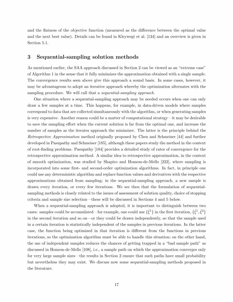
3 Sequential-sampling solution methods

As mentioned earlier, the SAA approach discussed in Section 2 can be viewed as an “extreme case”

of Algorithm 1 in the sense that it fully minimizes the approximation obtained with a single sample.

The convergence results seen above give this approach a sound basis. In some cases, however, it

may be advantageous to adopt an iterative approach whereby the optimization alternates with the

sampling procedure. We will call that a sequential-sampling approach.

One situation where a sequential-sampling approach may be needed occurs when one can only

draw a few samples at a time. This happens, for example, in data-driven models where samples

correspond to data that are collected simultaneously with the algorithm, or when generating samples

is very expensive. Another reason could be a matter of computational strategy—it may be desirable

to save the sampling effort when the current solution is far from the optimal one, and increase the

number of samples as the iterates approach the minimizer. The latter is the principle behind the

Retrospective Approximation method originally proposed by Chen and Schmeiser [44] and further

developed in Pasupathy and Schmeiser [185], although these papers study the method in the context

of root-finding problems. Pasupathy [184] provides a detailed study of rates of convergence for the

retrospective approximation method. A similar idea to retrospective approximation, in the context

of smooth optimization, was studied by Shapiro and Homem-de-Mello [222], where sampling is

incorporated into some first- and second-order optimization algorithms. In fact, in principle one

could use any deterministic algorithm and replace function values and derivatives with the respective

approximations obtained from sampling; in the sequential-sampling approach, a new sample is

drawn every iteration, or every few iterations. We see then that the formulation of sequential-

sampling methods is closely related to the issues of assessment of solution quality, choice of stopping

criteria and sample size selection—these will be discussed in Sections 4 and 5 below.

When a sequential-sampling approach is adopted, it is important to distinguish between two

cases: samples could be accumulated—for example, one could use {ξ1} in the first iteration, {ξ1, ξ2}in the second iteration and so on—or they could be drawn independently, so that the sample used

in a certain iteration is statistically independent of the samples in previous iterations. In the latter

case, the function being optimized in that iteration is different from the functions in previous

iterations, so the optimization algorithm must be able to handle this situation; on the other hand,

the use of independent samples reduces the chances of getting trapped in a “bad sample path” as

discussed in Homem-de-Mello [108], i.e., a sample path on which the approximation converges only

for very large sample sizes—the results in Section 2 ensure that such paths have small probability

but nevertheless they may exist. We discuss now some sequential-sampling methods proposed in

the literature.

17

3.1 Stochastic Approximation methods

Perhaps the most well-studied sequential sampling technique for stochastic optimization is the so-

called Stochastic Approximation (SA) method. As seen earlier, in its basic form SA is defined by

the recursive sequence

xk+1 := xk − αkηk, k ≥ 0, (15)

where −ηk is a random direction satisfying some properties—for example, the expectation of such

a direction should be a descent direction for the true function g—and αk is the step-size at iteration

k. The condition imposed on the sequence {αk} is that it goes to zero but not too fast, which is

usually formalized as∑∞

k=0 αk = ∞,∑∞

k=0 α2k < ∞. For constrained problems, xk+1 is defined as

the projection of xk − αkηk onto the feasibility set X.

Since the initial work by Robbins and Monro [200], great effort has been applied to the devel-

opment of both theoretical and practical aspects of the method. Robbins and Monro’s problem

was actually to find a zero of a given noisy function; Kiefer and Wolfowitz [129] applied the idea

to optimization and used finite-difference estimators of the gradient. The idea of using gradient

estimators constructed solely from function evaluations was further developed into a method called

Simultaneous Perturbation Stochastic Approximation; see Spall [230] for a detailed discussion. A

different line of work involves the use of ordinary differential equations to analyze the behavior

of SA algorithms; such an approach was introduced by Kushner and Clark [139] and elaborated

further in Kushner and Yin [140], see also Borkar and Meyn [31]. Andradottir [4] proposed a scaled

version of SA that aims at circumventing the problem of slow convergence of the original method

when the function being minimized is nearly flat at the optimal solution. Some developments in

SA have come from the application of this type of method in learning algorithms; see, for instance,

the book by Bertsekas and Tsitsiklis [24] and the work of Kunnumkal and Topaloglu [138] for a

more recent account.

Much of the effort in research on SA-type algorithms has focused on strategies that can speed

up the algorithm (in terms of improving the convergence) while keeping its adaptive nature. The

dilemma here is that, although the basic SA algorithm (15) can be shown to have optimal rate of

convergence O(1/k)—where k is the number of iterations—such rate is obtained for smooth and/or

strongly convex functions and an “optimal” choice of stepsizes, which are typically unknown in

practice. When non-optimal stepsizes are used, actual convergence can be very slow (see, e.g.,

Spall [230]), although Broadie et al. [33] have recently proposed some enhancements to the Kiefer-

Wolfowitz algorithm that show promising results in terms of practical performance.

An important development was provided by Polyak and Juditsky [197], who proposed a simple

but powerful idea: rather than looking at the iterates {xk} defined in (15), one should analyze the

average iterates

xk :=1

k

k−1∑i=0

xi.

Such a method also achieves the theoretical rate of convergence, but the averaging allows for more

18

robustness with respect to stepsizes. Earlier, Nemirovski and Yudin [169] had proposed averaging

the iterates using the stepsizes as follows:

xk :=

∑k−1i=0 αix

i∑k−1i=0 αi

, (16)

where the stepsizes αk are “longer” than those in the classical SA algorithm—for example, αk can

be of order k−1/2. The resulting algorithm was shown to be more robust with respect to stepsizes

and properties of the function being minimized. The idea of averaging is also present in other

variants of SA. For example, Dupuis and Simha [73] proposed a method whereby the stepsize αk

is constant for all k and the estimator ηk is given by a sample average. They used large deviations

theory to show convergence of the method and suggested a growth rate for the sample size.

In a different context and for the more structured case in which the integrand function G

is convex (although possibly nondifferentiable) a closely related method, called Stochastic Quasi-

Gradient (SQG), was developed in the seventies. The basic idea is still a recursion like (15), but

here the ηk is taken to be a stochastic quasigradient of G, that is, a vector satisfying

E[ηk|x0, . . . , xk

]= ∇g(xk) + bk

where ∇g(xk) denotes a subgradient of g at xk and {bk} is a sequence such that ‖bk‖ → 0. A review

of this technique can be found in Ermoliev [75]; discussion on practical aspects such as choice of

stepsizes, stopping rules and implementation guidelines are given by Gaivoronski [84] and Pflug

[189].

More recently, a new line of SA (or SQG) algorithms for convex problems has been proposed

based on the use of proximal-point techniques. Rather than using an iteration of the type (15),

these algorithms define the next iterate xk+1 as a suitable projection using proximal-type functions.

While the idea of using proximal-type functions had been studied earlier (see, e.g., Ruszczynski

[211]), the new methods allow for further enhancements. For example, the Mirror-Descent SA

method introduced by Nemirovski et al. [170] defines

xk+1 := Pxk(βkηk),

where ηk is an unbiased estimator of ∇g(xk), Px(·) is the prox-mapping defined as Px(y) =

argminz∈XyT (z − x) + V (x, z), {βk} is a sequence of stepsizes (which need not go to zero), V

is the prox-function V (x, z) = ω(z) − ω(x) − ∇ω(x)T (z − x), and ω(·) is a distance-generating

function, i.e., a smooth strongly convex function. Notice that this method generalizes the basic

SA algorithm, since the choice of ω(x) = (1/2)‖x‖22 (where ‖ · ‖2 denotes Euclidean norm) yields

the recursion (15). However, the flexibility in choosing the function ω(·) allows for exploiting the

geometry of the problem. In addition, the iterates are averaged as in (16). As demonstrated in

Nemirovski et al. [170], the resulting algorithm allows not only for more robustness with respect

to the parameters of the algorithm, but also for excellent performance in the experiments reported

19

in the paper; indeed, the error obtained with a fixed sample size is similar to that obtained with a

standard SAA approach corresponding to the same sample size, but the computational times are

much smaller than those with SAA. Lan [141] provided further enhancement to the mirror-descent

algorithm by introducing new sequences that aggregate the iterates; the resulting method—called

Accelerated SA—is shown to achieve optimal rate of convergence both in the smooth and non-

smooth cases.

Nesterov [171] proposed a primal-dual method which works in the dual space of the problem,

with the goal of preventing the weights of subgradients from going to zero. In the algorithm

(called Stochastic Simple Averages), the next iterate xk+1 is defined as xk+1 := Pγβk(ηk), where

ηk =∑k

t=1∇G(xt, ξt), Pβ(·) is the mapping defined as Pβ(s) = argminz∈X − sT z + βω(z), {βk}is a sequence of stepsizes (which need not go to zero), γ is a positive constant, and as before ω(·)is a distance-generating function. The algorithm is shown to have optimal rate in the sense of

worst-case complexity bounds.

3.2 Sampling-based algorithms for stochastic linear programs

A number of algorithms have been developed in the literature that exploit the special structures

of the specific class of problem they are applied to, and therefore can work well for that class

of problems. A set of such algorithms is rooted in the L-shaped method (Van Slyke and Wets

[235]), originally devised for two-stage stochastic linear programs. L-shaped method in stochas-

tic programming is commonly known as Benders’ decomposition (Benders [22]) in mixed-integer

programming and Kelley’s cutting plane algorithm in convex programming (Kelley [127], Hiriart-

Urruty and Lemarechal [106]). The L-shaped method achieves efficiency via decomposition by

exploiting the block structure of stochastic programs with recourse. The Stochastic Decomposition

method of Higle and Sen [100] is a sampling-based version the L-shaped method for stochastic linear

programs, using sampling-based cutting planes within the L-shaped algorithm. Infanger [120] and

Dantzig and Infanger [52] embed importance sampling techniques—which aim at reducing variance,

see Section 7.4 below—within the L-shaped method.

Specialized sampling-based algorithms have also been developed for the case of multistage

stochastic linear programs (MSSPs). Such models have been widely used in multiple areas such as

transportation, revenue management, finance and energy planning. A general MSSP for a problem

with T + 1 stages can be written as

min c0x0 + Eξ1 [Q1(x0, ξ1)]

subject to [MSSP]

A0x0 = b0.

x0 ≥ 0

20

The function Q1 is defined recursively as

Qt(x0, . . . , xt−1, ξ1, . . . , ξt) = min ctxt + Eξt+1 [Qt+1(x0, . . . , xt, ξ1, . . . , ξt+1)]

subject to (17)

Atxt = bt −t−1∑m=0

Bm+1xm,

xt ≥ 0

t = 1, . . . , T − 1. In the above formulation, the random element ξt denotes the random components

of ct, At, Bt, bt. Notice that we use the notation Eξt+1 [Qt+1(x0, . . . , xt, ξ1, . . . , ξt+1)] to indicate the

conditional expectation E [Qt+1(x0, . . . , xt, ξ1, . . . , ξt+1) | ξ1, . . . , ξt]. The function QT for the final

stage T is defined the same way as the general Qt in (17), except that it does not contain the

expectation term in the objective function.

Although the MSSP model fits the framework of (SP), the application of sampling methods

to that class of problems is more delicate. As discussed in Shapiro [219], a procedure whereby

some samples of the vector ξ := (ξ1, . . . , ξT ) are generated and the corresponding approximating

problems are solved exactly will not work well. It is not difficult to see why—the nested structure

of MSSP requires that the expectation at each stage be approximated by a sample average, which

cannot be guaranteed by simply drawing samples of ξ. To circumvent the problem, a conditional

sampling scheme, in which samples of ξt are generated for each sampled value of ξt−1, must be

used. The resulting structure is called a scenario tree. Of course, this implies that the number of

samples required to obtain a good approximation of MSSP grows exponentially with the number

of stages. Thus, exact solutions of the approximating problem often cannot be obtained.

To address the problem of large scenario trees, some algorithms have been proposed whereby

sampling of scenarios from the tree is incorporated into an optimization procedure. Note that the

input to these algorithms is a scenario tree, so the sampling that is conducted within the algorithm

is independent of any sampling that may have been performed in order to generate a scenario

tree. Examples of such algorithms are the Stochastic Dual Dynamic Programming (Pereira and

Pinto [188], see also Shapiro [220] for further analysis), CUPPS (Chen and Powell [46]), Abridged

Nested Decomposition (Donohue and Birge [64]), and ReSa (Hindsberger and Philpott [105]). A

convergence analysis of this class of algorithms is provided by Philpott and Guan [193].

3.3 Sampling-based algorithms for “black-box” problems

Many sampling-based methods have been proposed for problems where little assumption is made

on the structure of the function being optimized and the feasibility set X, which can be discrete or

continuous. Such algorithms guide the optimization based solely on estimates of function values at

different points. This setting is often referred to as simulation optimization in the literature. There

is vast amount of work in that area, and some excellent surveys have been written; see, for instance

Fu [82], Andradottir [5] and Chen et al. [43], to which we refer for a more comprehensive discussion.

21

We note that this is a growing area of research; as such, new methods have been investigated since

the publication of these reviews. We provide here a brief overview of the sampling-based black-box

algorithms.

The challenge in stochastic black-box algorithms is two-fold: on the one hand, the lack of

problem structure requires a strategy that balances the effort between visiting different parts of the

feasibility set versus gaining more information around the solutions that have shown to be more

promising—this is the well-known dilemma of exploration vs. exploitation present in deterministic

optimization as well. Often this is accomplished by the use of some random search procedure that

makes it more likely to visit the points around the most promising solutions. On the other hand,

the fact that the objective function cannot be evaluated exactly creates another layer of difficulty,

since one cannot be 100% sure that a certain solution that appears promising is indeed a good

solution.

Some of the algorithms proposed in the literature incorporate sampling techniques into global

search methods originally developed for deterministic optimization. Examples of such work include

algorithms based on simulated annealing (Alrefaei and Andradottir [3]), genetic algorithms (Boesel

et al. [30]), cross-entropy (Rubinstein and Kroese [208]), model reference adaptive search (Hu

et al. [116]), nested partitions (Shi and Olafsson [228]), derivative-free nonlinear programming

algorithms (Barton and Ivey [12], Kim and Zhang [130]), and branch-and-bound methods (Norkin

et al. [174, 175]). Algorithms have also been proposed based on the idea of building a response

surface for the function value estimates and using some methodology such a trust-region approach

to guide the optimization; examples include Angun et al. [7], Barton and Meckesheimer [13], Bastin

et al. [14], Bharadwaj and Kleywegt [26] and Chang et al. [40]. The issues of sample size selection

and stopping criteria arise here as well—we will discuss more about that in Sections 4 and 5.

Ranking-and-selection methods aim at guaranteeing that the best solution is found with some

pre-specified probability, but such techniques are only practical if the number of feasible alternatives

is relatively small. Some recent methods, such as the Industrial Strength COMPASS method

proposed by Xu et al. [242], aim at combining features of random search (for exploration), local

search (for exploitation) and ranking-and-selection (for probabilistic guarantees).

Another class of algorithms relies on the idea of Bayesian formulations for the optimization

problem. Generally speaking, in such methods a prior probability distribution (often a Normal

distribution) is placed on the value of the alternatives being evaluated; samples corresponding to

one or more alternatives are collected, the parameters of the prior distribution are updated in a

Bayesian fashion based on the observed values, and the process is repeated until some stopping

criterion is satisfied. A key element in such algorithms is a method to decide which alternative(s)

should be sampled in each iteration. Examples of such work—which include methods based on

optimization via Gaussian processes, stochastic kriging, and knowledge gradient, among others—

are Ankenman et al. [8], Chick and Frazier [47], Chick and Inoue [48], Frazier et al. [77, 78], Huang

et al. [118] and Scott et al. [214].

In the context of dynamic discrete problems, stochastic optimization problems are closely related

22

to Markov decision processes (MDPs). Sampling-based methods have been proposed in that area

as well. For example, Chang et al. [39] proposed an adaptive sampling algorithm that approximates

the optimal value of a finite-horizon Markov decision process (MDP) with finite state and action

spaces. The algorithm adaptively chooses which action to sample as the sampling process proceeds

and generates an asymptotically unbiased estimator of the value function.

4 Assessing solution quality

We now turn our attention to how to assess the quality of a solution to a stochastic optimization

problem. In this section, we again focus on the class of (SP) with K = 0 and will return to problems

with stochastic constraints in Section 6. When assessing solution quality, we denote the candidate

solution as x ∈ X. This candidate solution is fixed, and our aim is to figure out if it is optimal

or near-optimal. Determining if a solution is optimal or near optimal plays a prominent role in

optimization theory, algorithms, computation, and practice. Note that the solution x ∈ X can be

obtained by any method. For instance, it can be obtained by the SAA approach by letting x = xN

for some sample size N . Alternatively, it can be obtained by running a Monte Carlo sampling-based

algorithm (e.g., the general Algorithm 1 in Section 1, or any of the methods discussed in Section

3) for k iterations and letting x = xk. Other approaches for obtaining the candidate solution are

possible. In this section, we first review methods that are independent of the algorithm used to

obtain the solution. As such, in Sections 4.1 and 4.2, we assume that if Monte Carlo sampling is

used to obtain the candidate solution, this is done independently of the Monte Carlo sampling to

assess solution quality. Note that there are also ways to assess solution quality within a specific

algorithm, typically using the information (such as subgradients, etc.) obtained throughout the

algorithm. We briefly review these in Section 4.3.

4.1 Bounding the optimality gap

One of the classic approaches for assessing solution quality in optimization is to bound the candidate

solution’s optimality gap. If the bound on the optimality gap is sufficiently small, then the candidate

solution is of high quality. In deterministic optimization, because the objective function at candidate

solution x ∈ X can typically be calculated, bounding x’s optimality gap amounts to finding lower

bounds on the optimal objective function value. These lower bounds are often obtained through

relaxations; for instance, via integrality, Lagrangian or semidefinite programming relaxations. In

stochastic optimization, Monte Carlo sampling can be used to obtain (statistical) lower bounds.

This approach can also be viewed as a type of relaxation in the sense that instead of considering

the whole distribution, we look at a subset dictated by the sample.

Recall that the optimality gap of x is g(x)− ν∗. The optimal value ν∗ is not known but can be

bound by the bias result given in (8): E [νN ] ≤ ν∗. In essence, instead of using “all” information

on ξ, using a subset of observations that are present in the sample leads to, on average, over-

optimization. This is in line with optimistic objective function values obtained using “relaxed”

23

problems in deterministic optimization. Therefore, an upper bound on the optimality gap of x,

E [G(x, ξ)]− E [νN ], can be estimated via

GN (x) := gN (x)− νN . (18)

From this point on, we will refer to (18) as a point estimator of the optimality gap of x ∈ X

rather than an estimator of its upper bound. When viewed as an estimator of optimality gap,

GN (x) is biased; i.e., E [GN (x)] ≥ g(x)− ν∗. While there are different ways to calculate the above

optimality gap estimator, a basic version uses the same independent and identically distributed

(i.i.d.) observations ξ1, ξ2, . . . , ξN from the distribution of ξ for both terms in (18). That is, given

an arbitrary realization {ξ1, ξ2, . . . , } of the random vector ξ, we compute

GN (x) := gN (x, ξ1, . . . , ξN )− νN (ξ1, . . . , ξN ), (19)

where the notation νN (ξ1, . . . , ξN ) emphasizes that this quantity corresponds to the optimal value

of problem (4) for the particular realization {ξ1, . . . , ξN}.The use of the same observations in both terms of (19) results in variance reduction via the use

of common random variates. As indicated in Section 2.2, νN may not be asymptotically normal (see

(10)). Therefore, GN (x) is typically not asymptotically normal, complicating statistical inference.

This difficulty can be circumvented by employing a “batch-means” approach commonly used in

the simulation literature. That is, multiple independent estimators GkN (x) are generated using

NG “batches” of observations ξk1, ξk2, . . . , ξkN , k = 1, 2, . . . , NG , and these GkN (x) are averaged to

obtain a point estimator of the optimality gap

G(x) :=1

NG

NG∑k=1

GkN (x). (20)

The sample variance is calculated in the usual way, s2G := 1

NG−1

∑NGk=1

(GkN (x)− G(x)

)2. An

approximate (1−α)-level confidence interval estimator on the optimality gap of x is then obtained

by [0, G(x) +

zαsG√NG

], (21)

where zα denotes a 1 − α quantile from a standard Normal distribution. The resulting point

estimator (20) and interval estimator (21) are called the Multiple Replications Procedure (MRP)

estimators. MRP was developed by Mak, Morton, and Wood [158] and the idea of using νN to

bound ν∗ was used by Norkin et al. [175] within a sampling-based branch-and-bound framework.

Notice that the confidence interval above is a one-sided (upper) interval. This is in an effort to

obtain a more conservative estimate which can help, for instance, when used as a stopping rule (see

e.g., (36) in Section 5.3).

The MRP confidence interval (21) for the optimality gap of x is asymptotically valid when the

batches {ξk1, ξk2, . . . , ξkN}, k = 1, 2, . . . , NG , are i.i.d., coupled with the consistency of the variance

24

estimator s2G of σ2

G = Var[GN (x)], through the Central Limit Theorem (CLT)

√NG [G(x)− E [GN (x)]]

d→ Normal(0, σ2G).

We assume that G(x, ξ) has finite second moments for all x ∈ X in order to invoke the CLT.

Notice that the CLT holds even when observations within each batch are obtained in a non-i.i.d.

fashion. Non-i.i.d. sampling schemes that produce unbiased estimators for a given solution x, i.e.,

E[N−1

∑Nj=1G(x, ξkj)

]= E [G(x, ξ)], k = 1, 2, . . . , NG , can be used to generate each batch of obser-

vations. This fact can be used to obtain variants of MRP that are aimed to reduce variance and/or

bias. See, for instance, Bayraksan and Morton [20] for one such variation that uses randomized

quasi-Monte Carlo sampling to generate the batches in an effort to reduce variance.

With an asymptotically valid confidence interval, the output of MRP is a probabilistic statement

on the optimality gap of x of the form

P

(g(x)− ν∗ ≤ G(x) +

zαsG√NG

)≈ 1− α.

Notice that the bias of νN results in an overestimation of the optimality gap and this can lead to

wider confidence levels for small sample sizes. Such conservative coverage has been observed for

some problems in the computational results by Bayraksan and Morton [19] and Partani [182].

A major advantage of MRP is its wide applicability. Problem (SP) can contain discrete or con-

tinuous decisions and in two-stage stochastic programs with recourse, the discrete and/or continuous

decisions can be present at any stage. The problem can have nonlinear terms in the objective or

constraints; neither X nor g need to be convex. It is explicitly assumed, however, that the samples

of ξ can be generated and the function evaluations G(x, ξ) can be performed. As mentioned above,

we also assume finite second moments of G(x, ξ). The most restrictive aspect of MRP is that it

requires solution of NG SAA problems (4) to obtain estimates of νN in GN (x). (In implementation,

NG is typically taken to be around 20-30 to induce the CLT.) The ability to solve SAA problems

and the computational effort required depends on the class of problem MRP is applied to. Note

that the SAA problems can be solved using any specialized algorithm for the problem at hand. We

also note that approximate methods that yield lower bounds on νN can be used instead but with

weakened bounds and more conservative optimality gap estimators. The framework to implement

MRP is relatively simple and step by step instructions can be found, for instance, in Bayraksan and

Morton [20]. Applications of MRP in the literature include supply chain network design (Santoso

et al. [213]), financial portfolio models (Bertocchi et al. [23], Morton et al. [162]), stochastic vehicle

routing problems (Kenyon and Morton [128], Verweij et al. [236]), scheduling problems (Morton

and Popova [161], Turner et al. [234]), and a stochastic network interdiction model (Janjarassuk

and Linderoth [121]).

Typically, MRP can be performed with modest computational effort. In cases where computa-

tional effort becomes prohibitive (because we solve NG SAA problems each of size N), an alternative

way to obtain optimality gap point and interval estimators is by using single or two replications

25

(Bayraksan and Morton [19]). In the Single Replication Procedure (SRP), NG = 1 and the point

estimator of optimality gap is simply given by (18). A major difference between MRP and SRP is

the variance estimator. In MRP, the sample variance of NG gap estimators GkN (x), k = 1, 2, . . . , NG

is calculated. In SRP, with NG = 1, this is not possible. In order to motivate the variance estimator

of SRP, let us rewrite (18) as

GN (x) =1

N

N∑j=1

(G(x, ξj)−G(xN , ξ

j)),

where as before xN denotes the optimal solution to the sampling problem minx∈X gN (x) with

optimal value νN . Viewing GN (x) as the sample average of the observations G(x, ξj)−G(xN , ξj),

j = 1, 2, . . . , N , the sample variance estimator is calculated as

s2G :=

1

N − 1

N∑j=1

[(G(x, ξj)−G(xN , ξ

j))− GN (x)

]2, (22)

where we have omitted the dependence of sG on N and x to simplify the notation. Note that x is

fixed but xN is obtained by optimizing a sample mean, i.e., xN depends on ξ1, . . . , ξN . Therefore,

the usual statistical analysis of sample means does not apply. Nevertheless, it is still possible to

obtain asymptotically valid (1− α)-level confidence intervals[0,GN (x) +

zαsG√N

]. (23)

Asymptotic validity of the confidence interval in (23) means that

lim infN→∞

P

(g(x)− ν∗ ≤ GN (x) +

zαsG√N

)≥ 1− α.

To establish the above inequality, a key component is to ensure the consistency of the variance

estimator of SRP. Suppose that E[supx∈X G

2(x, ξ)]< ∞, which guarantees the second moments

are finite. Consistency of sG means that asymptotically (as N →∞) we have that

infx∈S∗

σ2x(x) ≤ s2

G ≤ supx∈S∗

σ2x(x) w.p.1, (24)

where σ2x(x) := Var[G(x, ξ)−G(x, ξ)].

Note that when there is a unique optimum solution, i.e., S∗ = {x∗}, (24) turns into the usual

strong consistency result for the variance estimator s2G, i.e., limN→∞ s

2G = σ2

x(x∗) w.p.1. When there

are multiple optima, however, the variance of G(x, ξ)−G(x, ξ) might change at each x ∈ S∗ (recall

that x is fixed). The consistency result in (24) states that the variance estimator is guaranteed

to be within a minimum and maximum of variances in the set of optimal solutions. Bayraksan

and Morton [19] provide a set of conditions under which (24) is satisfied, including i.i.d. sampling,

26

Input: x ∈ X; a method to generate observations; a method to solve (2)

Output: A point estimator (e.g., GN (x)) and a (1− α)-level approximate confidence interval estimator ofE [G(x, ξ)]− ν∗ (e.g., of the form [0,GN (x) + εα], where εα denotes the sampling error)

Observations Point Estimator Variance Estimator Sampling Error

MRP

G(x) =

NG∑k=1

GkN (x)

NGs2G =

NG∑k=1

(GkN (x)− G(x)

)2NG−1

zαsG√NG

ξk1, ξk2, . . . , ξkN ,k = 1, 2, . . . , NG

SRP ξ1, ξ2, . . . , ξN GN (x)

s2G =

N∑j=1

[(G(x, ξj)−G(xN , ξ

j))− GN (x)

]2N−1

zαsG√N

2RP

G′(x) =

2∑k=1

GkN (x)

2s2

′G =

2∑k=1

s2G,k

2

zαs′G√

2N

ξ11, ξ12, . . . , ξ1N ,ξ21, ξ22, . . . , ξ2N

Notes: GN (x) is given in (18). 2RP averages two SRP point and variance estimators.

NG of MRP is typically chosen to be 20-30 in practice.

Table 2: Summary of Procedures for Optimality Gap Estimation

X 6= ∅ and compact, and G(·, ξ) is continuous, w.p.1. These conditions are satisfied, for instance,

by two-stage stochastic linear programs with relatively complete recourse (for each x ∈ X, the

second-stage problem is feasible). The i.i.d. assumption is relaxed in Drew [66], who extends the

result to the case where the generated vectors are Quasi-Monte Carlo sequences “padded” with

Latin Hypercube sampling; see Sections 7.2 and 7.3.

Computational results show that the coverage probability of the SRP confidence interval does

not have the same conservative results as MRP. In fact, for some problems, SRP can have unde-

sirably low coverage probability, i.e., the proportion of times in which the interval given by (23)

actually contains the true gap g(x)− ν∗ is smaller than 1− α. In practice, it is better to use two

replications instead of one. This is referred to as 2 Replication Procedure (2RP), or the Averaged 2

Replication Procedure (A2RP). In 2RP, NG = 2, and so, two independent estimates of optimality

gap GkN (x) and sample variance s2G,k, k = 1, 2 are obtained. Then, these are averaged to obtain

G′(x) =1

2

2∑k=1

GkN (x) and s2 ′G =

1

2

2∑k=1

s2G,k.

The (1−α)-level approximate confidence interval is obtained in a similar way, i.e.,[0, G′(x) +

zαs′G√2N

].

The same conditions to ensure asymptotic validity of SRP confidence interval ensure asymptotic

validity of 2RP interval estimator. It is also possible to increase the number of replications but

computational results suggest that using two replications is typically sufficient in practice (Bayrak-

san and Morton [19]). Table 2 summarizes the procedures outlined above to obtain optimality gap

point and interval estimators for a given solution x.

Instead of using common random variates as in the above procedures, it is possible to use one

sample to estimate g(x) and another to estimate the lower bound E [νN ] on ν∗. Let NU denote

27

the sample size to estimate E [G(x, ξ)] via the sample mean U = N−1U

∑NUj=1G(x, ξj). Similarly,

let NL be the number of batches to estimate E [νN ] via L = N−1L

∑NLj=1 ν

jN . These two estimators

subtracted from one another, U − L, gives a point estimator of optimality gap. Due to variation,

this estimate can be negative, so, max{U − L, 0} can be used instead. To form an asymptotically

valid interval estimator, the sampling errors of U and L are calculated separately, invoking the

CLT, and are combined using the Boole-Bonferroni inequality (for details, we refer the reader to

Section 3.1 of Mak et al. [158]). Because estimation of E [G(x, ξ)] is computationally cheaper, NU

can be chosen to be very large. The computational bottleneck is again the solution of NL SAA

problems and NL is taken to be 20− 30 to induce the CLT. When the correlation between G(x, ξ)

and νN is low, using a very large value of NU can result in an overall sampling error less than the

one using common random variates. However, when there is a strong positive correlation between

G(x, ξ) and νN , we may expect significant variance reduction when using the common random

variates version of MRP in Table 2. For computational results on these versions, see, for instance

Mak et al. [158], Kenyon and Morton [128] and Verweij et al. [236].

When the point or interval estimator of the optimality gap of a candidate solution turns out to

be large, this could be due to (i) the candidate solution being far from optimal, (ii) variability is

large, or (iii) bias is large. Suppose the candidate solution is indeed a high-quality solution. We can

still have large estimators due to variance and/or bias and this can hinder our ability to validate that

it is in fact a high-quality solution. For variance reduction, above, we mentioned using alternative

sampling techniques to reduce variability in MRP, SRP, and 2RP estimators. The issue of bias

in optimality gap estimation, on the other hand, is analogous to weak bounds in deterministic

optimization. For instance, in integer programming, sometimes when an optimal solution is found,

it takes significant computational effort to prove its optimality due to weak bounds. Similarly, bias

results in a weak lower bound, on average, on ν. Because bias decreases as N increases, one way to

decrease bias is to simply increase N when calculating νN . However, this can be computationally

burdensome and the decrease in bias can be slow—of order O(N−1/2) as discussed in Section 2.2.

For bias reduction, Partani [182] and Partani et al. [183] present an adaptive version of MRP,

which is motivated by the generalized jacknife estimators in statistics (Gray and Schucany [94]).

Stockbridge and Bayraksan [232] use stability results in stochastic programming to reduce bias

in 2RP estimators by partitioning the 2N observations into two groups of N by minimizing the

distance between the resulting empirical distributions. We end by noting that some sampling

methods aimed to reduce variance, like Latin Hypercube sampling, have been observed to reduce

bias as well, see, e.g., the computational results in Freimer et al. [79]. These sampling methods

spread the observations more evenly than random sampling. Consequently, it can be less likely

to over-optimize, resulting in a reduction in bias (recall the discussion in the paragraph preceding

equation (18)).

28

4.2 Testing optimality conditions

Another classic approach to assessing solution quality in optimization is determining whether a

solution satisfies conditions that ensure optimality. For instance, Karush-Kuhn-Tucker (KKT)

conditions provide necessary and sufficient conditions for optimality for a class of problems. Be-

cause we are dealing with a stochastic optimization problem, the function values and (sub)gradients

needed for evaluation of optimality conditions are typically not readily available and need to be

estimated via Monte Carlo sampling. For example, a class of two-stage stochastic linear programs

with recourse can be viewed as (sub)differentiable convex optimization problems and assessment of

solution quality via statistical evaluation of KKT conditions have been studied for this class of prob-

lems. Of course, the problem class is larger than a subset of two-stage stochastic linear programs

with recourse. We note that evaluation of KKT conditions based on Monte Carlo sampling-based

estimates, compared to a procedure like MRP, is more restrictive in terms of the problem class it

applies to. Below, we sketch out one way to evaluate KKT conditions in the presence of Monte

Carlo sampling-based estimators of function values and gradients and the difficulties that arise in

this statistical evaluation of KKT conditions.

Suppose g(·) is differentiable at the candidate solution x ∈ X and also G(·, ξ) is differen-

tiable at x, w.p.1, and that it is possible to interchange expectation and differentiation; i.e.,

∇g(x) = E [∇xG(x, ξ)] . In two-stage stochastic linear programs with recourse, for instance, these

assumptions can hold when the distribution of ξ is continuous. Given an i.i.d. sample ξ1, ξ2, . . . , ξN

from the distribution of ξ, a Monte Carlo sampling-based estimator of ∇g(x) can be formed by

∇gN (x) =1

N

N∑j=1

∇xG(x, ξj). (25)

If ∇xG(x, ξ) has finite second moments, then, by the CLT,√N [∇gN (x)−∇g(x)]

d→ Normal(0,Σ),

where Σ is the covariance matrix of ∇xG(x, ξ), assumed to be nonsingular. Let [·]′ denote the

transpose of its argument. The sample covariance matrix

ΣN =1

N − 1

N∑j=1

[∇xG(x, ξj)−∇gN (x))

] [∇xG(x, ξj)−∇gN (x))

]′(26)

provides an unbiased and consistent estimator of Σ. Given Monte Carlo sampling-based estimators

∇gN (x) and ΣN of ∇g(x) and Σ, respectively, our aim is to evaluate statistically if x satisfies the

KKT conditions. Let us now review the KKT conditions.

Suppose X is composed of m1 equality and m−m1 inequality constraints

X = {x : hi(x) = 0, i = 1, 2, . . . ,m1; hi(x) ≤ 0, i = m1 + 1, . . . ,m}.

Suppose further that hi(·), i = 1, . . . ,m are continuously differentiable and g(·) is differentiable at

optimal solution x∗ ∈ X. Let I(x) = {i : hi(x) = 0, i = m1 + 1, . . . ,m} denote the index set of

29

inequality constraints that are active at x. We assume that any necessary constraint qualification

conditions are satisfied. One way to write the KKT conditions is

−∇g(x∗) ∈ NX(x∗), (27)

where NX(x∗) denotes the normal cone of X at x∗, written as

NX(x∗) =

z ∈ Rn : z =

m1∑i=1

αi∇hi(x∗) +∑

i∈I(x∗)

αi∇hi(x∗), where αi ≥ 0 for i ∈ I(x∗)

.

The aim is to test whether x satisfies KKT conditions; i.e., if −∇g(x) ∈ NX(x) (null hypothesis

H0) or not (alternative H1). Assume that all conditions satisfied at x∗ such as differentiability are

satisfied at x. One way to do this is to determine the distance between the point −∇g(x) and the

set NX(x). Because ∇g(x) is not known, we replace it by its Monte Carlo sampling-based estimator

in (25). Then, the test statistic can be defined as

TN (x) = dist(−∇gN (x), NX(x)), (28)

where dist(a,B) denotes the distance between point a and set B. The test statistic can be obtained

in different ways. For instance, one can use

TN (x) = N minz∈NX(x)

[∇gN (x)− z]′Σ−1N [∇gN (x)− z]. (29)

With nonsingular ΣN , (29) is a quadratic programming problem. Suppose strict complementarity

condition holds (αi > 0 for i ∈ I(x)). Under the null hypothesis, (29) converges in distribution to

a chi-squared random variable with dx − (m1 + |I(x)|) degrees of freedom. Then, a large p-value,

close to 1, suggests a high quality solution whereas a small p-value indicates that either x is far

from optimal or there is a large error in the estimation. Recall that p-value can be calculated by

P (Y ≥ TN (x)), where Y is distributed chi-squared with dx − (m1 + |I(x)|) degrees of freedom.

The above discussion is based on Shapiro and Homem-de-Mello [222], to which we refer for a

more detailed description of the statistical methods used to test the hypotheses. There are also

other papers that study approaches to test KKT conditions under uncertainty. For example, Higle

and Sen [101] use KKT conditions within the framework of the stochastic decomposition algorithm

for a class of two-stage stochastic linear programs and use bootstrapping to assess the variability

in their estimates; see also Higle and Sen [102]. Note that in many cases—both in two-stage

stochastic programs and in simulation—g(·) is not differentiable but only subdifferentiable. Similar

ideas to the statistical tests described above can be used in the subdifferentiable case, as discussed

by Linderoth et al. [152] who also present extensive computational results. We refer the readers to

Shapiro [218] for convergence of Monte Carlo sampling-based estimators of subdifferentials and for

alternative test statistics of type (28).

30

We end this section by noting that above methods assume deterministic constraints. In the case

with stochastic constraints, Bettonvil et al. [25] develop a series of hypotheses tests for verification

of KKT conditions. Royset [204] uses the so-called optimality function, which has two parts, one

that is related to feasibility of the candidate solution with respect to the stochastic constraints and

the other testing the more general Fritz-John conditions (similar to KKT conditions) for optimality.

4.3 Assessing solution quality for specific sampling-based algorithms

Above, we discussed how to assess the quality of a given solution which may be obtained in any

way. In many cases, solutions are produced sequentially as part of an algorithm and assessment

of quality must be made throughout the algorithm to determine a stopping time, or sometimes

to aid the next iteration. In this section, we briefly mention some of these methods. Note that

for a given x ∈ X, typically, estimation of E [G(x, ξ)] is relatively easier compared to estimating a

lower bound on ν∗ (for a minimization problem). Many sampling-based algorithms produce such

bounds throughout the algorithm, so, an estimator of a lower bound on ν∗ can be obtained more

efficiently within a specific algorithm. Lan et al. [142] develop a lower bound for the mirror de-

scent SA algorithm using the gradient estimates obtained throughout the algorithm. This lower

bound solves a lower-approximating linear program for a convex problem, hence is computationally

cheaper than solving an SAA problem, but it can be looser than νN on average. Similar ideas using

duality have been proposed earlier to obtain a statistical lower bound within the stochastic de-

composition method by Higle and Sen [101, 102] and improved via quadratic programming duality

for “in-sample” tests in Higle and Sen [103]. We also point to other work that uses Monte Carlo

sampling-based versions of lower bounds obtained in sampling-based adaptations of deterministic

cutting plane algorithms: Higle and Sen [101] use bootstrapping to check verification of general-

ized KKT conditions in stochastic decomposition; Glynn and Infanger [89] provide an asymptotic

analysis of the bounds used in the sampling-based cutting plane algorithm for two-stage stochastic

linear programs described in Dantzig and Glynn [53], Dantzig and Infanger [54] and Infanger [120];

and Homem-de-Mello et al. [111] discuss statistical stopping criteria in the context of the SDDP

algorithm for multistage stochastic linear programs. When |X| is finite and moderate, the estimator

in Ensor and Glynn [74] for a grid-search algorithm can be viewed as a lower bound on ν∗.

5 Choice of sample sizes

An important question when using Monte Carlo sampling-based algorithms is what sample size is

required to obtain a high-quality solution. For instance, one might be interested in determining

a sample size such that the solution obtained via an SAA approach, xN , is optimal with a high

probability. Estimates of sample sizes for this purpose have been obtained using large deviations

theory for a class of problems. In Section 5.1, we briefly review these. A related question concerns

the stopping rules for sampling-based algorithms. When should these algorithms stop in order to

have a high-quality solution? This also determines—in an indirect way—the sample sizes needed

31

to obtain a high-quality solution. Choice of sample sizes may also affect the performance of a

specific sampling-based algorithm. Is there a way to allocate the sample sizes within iterations of

an algorithm to obtain high-quality solutions quickly? In the remainder of this section, we discuss

answers to these questions. In Section 5.2 we review sample size selection strategies and in Section

5.3, we review stopping rules for sampling-based algorithms to have a priori control on the quality

of solutions obtained.

5.1 Theoretical sample size estimates

The rates of convergence discussed in Section 2.2 provide ways to estimate sample sizes to solve

a stochastic optimization problem with a given accuracy via an SAA approach. These estimates

have been derived using large deviations theory (Stroock [233]) in a series of papers by Shapiro and

Homem-de-Mello [223], Shapiro et al. [226] and Kleywegt et al. [134], see also Ahmed and Shapiro

[1]. We briefly review these here; for a more detailed summary we refer the readers to Shapiro et al.

[227].

Let Sε and SεN denote the set of ε-optimal solutions to the original problem (SP) and its SAA

(4). For a class of problems, under assumptions such as the existence of appropriate moment

generating functions, given 0 ≤ δ < ε,

1− P (SδN ⊂ Sε) ≤ Ce−Nβ (30)

for two constants C, β > 0; see also (14). These constants depend on the problem characteristics

and the values of δ and ε (we suppress any dependence for notational simplicity). The expression

in (30) states that the probability that a δ-optimal solution to SAA is an ε-optimal solution to the

original problem goes to 1 exponentially fast. Setting the right-hand side of (30) to be less than or

equal to a desired value of α and solving for N , the sample sizes

N ≥ β−1 ln

(C

α

)(31)

guarantee that the probability of obtaining ε-optimal solutions via solving an SAA problem with

δ precision is at least 1− α. Even with exponential convergence, if β is small, convergence can be

slow and the sample size estimate may be large.

Suppose X is finite. This is the case when the decisions to be made are discrete. In simulation,

for instance, one might like to determine an optimal number of servers or buffer size, for which

decisions are discrete. In this case, C = |X| and β is obtained as a minimal large deviations

exponential decay rate. By using a bound on β, the sample size estimate in (31) turns to

N ≥ 3σ2max

(ε− δ)2ln

(|X|α

), (32)

where σ2max = maxx∈X\Sε Var[G(x∗, ξ) − G(x, ξ)] for an optimal solution x∗ ∈ S∗. Let us now

32

examine the above sample size estimate. When the sampling problems are solved to optimality,

i.e. δ = 0, the sample size estimate (32) grows proportional to 1/ε2 as higher-quality solutions are

demanded. On the other hand, as δ approaches ε, the sample sizes grow. As can be expected, the

higher the variability in the problem, the higher the sample sizes need to be. The estimate (32)

also indicates that the sample sizes grow logarithmically in |X| and α. For example, with dx binary

decisions, the size of solution set |X| = 2dx may be very large, but the sample size only grows

proportional to dx. The estimate (32) is typically too conservative for practical purposes and may

be hard to estimate; for instance, estimating σ2max can be difficult.

When X is bounded but not finite, by reducing X to an “appropriate” finite subset Xν we

can obtain similar sample size estimates to solve the original problem to an ε accuracy. Here,

“appropriate” means that for any x ∈ X there exists an xν ∈ Xν such that ‖x− xν‖∞ ≤ ν. Note

that the set X has finite diameter D := supx,y∈X ‖x − y‖∞, so we can choose Xν such that it

has at most (D/ν)dx elements. If, further, the expectation g(x) is Lipschitz continuous on X with

Lipschitz constant L, then it is possible to show that the sample size estimate analogous to that in

(32) is

N ≥ 12σ2max

(ε− δ)2

(dx ln

2DL

ε− δ− lnα

).

For piecewise linear convex stochastic programs with finite Ξ and sharp, unique optimum

Shapiro et al. [226] introduce a condition number to explain the sample size needed for SAA to find

an optimal solution, by using exponential rates of convergence and characteristics of this class of

problems. When the condition number is low, the problems can be considered well-conditioned for

solving via SAA and when the condition number is high, one may expect larger sample sizes to

obtain high-quality solutions. Their analysis suggests that problems that have high variability and

flat objective functions around the optimal solution are ill-conditioned.

5.2 Allocation of sample sizes

The theoretical sample size estimates presented in Section 5.1 aim to determine a minimal sample

size for solving a single SAA problem to obtain high-quality solutions with a desired probability.

Now we shift focus to Monte Carlo sampling-based methods. Ideally, we would like to have a

procedure to automatically choose appropriate sample sizes in each iteration of a sampling-based

algorithm.

The main idea behind sample size allocation schemes is to allocate a minimal number of samples

while maintaining high accuracy of the approximations. The larger the sample sizes, the better

the approximation but the higher the computational cost. We already know that, at a minimum,

the sample sizes must tend to infinity for asymptotic properties such as consistency of the optimal

values to hold. By strategically allocating a sequence of samples, could we maximize, or at least

increase, the rate of convergence? Is there a way to allocate the sample sizes in order to minimize

the computational effort within a specific sampling-based algorithm?

Before looking at a strategic allocation of sample sizes, we can study the rate at which sample

33

sizes must grow. As we mentioned above, the sample sizes must grow in order to have consistent

estimators but at what (minimal) rate must they grow to ensure this? Homem-de-Mello [108]

investigates this question to ensure consistency of the objective function estimator in variable-

sample methods, and derives associated error statements in the spirit of the law of the iterated

logarithm. Under appropriate conditions, linear and superlinear growth of sample sizes with respect

to the iteration number k (e.g., the sample size Nk at iteration k satisfy Nk ≥ ck for some c > 0) as

well as a subset of sublinear sample sizes (e.g., Nk grows of O(√k)) ensure consistency. However,

a sublinear growth of O(log k) requires more stringent conditions to ensure consistency. Next, we

turn our attention to strategic sample size allocation.

The sample size allocation schemes often use one of two main computational objectives and/or

constraints: (a) to minimize expected total computational cost or total computational cost per run,

or (b) assume a fixed computational budget B and try to do the best within this budget, although in

the second case, B is often taken to infinity to provide asymptotically optimal sampling schemes.

On the convergence of desired quantities, we see that most research focuses on (i) efficient/fast

convergence of limit points of solutions {x∗n} to an optimal solution and some on (ii) convergence

of certain quantities (e.g., νN or the true objective function evaluated at xN ) to optimal value ν∗

by judicious sample size allocations. These two broad categorizations of computational cost and

consistency properties are often mixed and studied from both theoretical and practical points of

view for different classes of sampling-based algorithms. Other similar goals are possible.

On the computational objective (a)—minimizing expected total computational cost—we point

to, for instance, the works of Byrd et al. [35], Polak and Royset [196], and Royset [205] for different

sampling-based methods. Byrd, Chin, Nocedal, and Wu [35] present ways to dynamically allocate

sample sizes within a stochastic gradient method (both pure gradient and a Hessian-free Newton’s

method with conjugate gradients). Their method increases the sample size when the variance

estimate of the gradient is sufficiently large. When this condition is triggered, a larger sample size

is obtained in an effort to satisfy an estimated descent condition. Byrd et al. [35] also provide

theoretical analysis on an idealized version of their practical dynamic pure stochastic gradient

method. They show that if the sample sizes grow geometrically with iteration number k, that

is, Nk = dake for some a > 1, then the expected total work to obtain an ε-optimal solution is

O(1/ε) for uniformly convex objective functions. Another approach to computational objective (a)

is to formulate a discrete-time optimal control problem to minimize the expected computational

cost of obtaining a solution to a sequence of SAA problems. For stochastic nonlinear programs,

Polak and Royset [196] propose a control problem that aims to minimize the computational effort

required to reduce an initial optimality gap by a prespecified fraction in the context of so-called

diagonalization schemes. Recent work by Royset [205] extends on this approach to characterize

sample size selection policies when solving smooth stochastic programs. A dynamic program is

solved to determine the sample sizes to use for each SAA problem as well as the computational

effort that should be expended to solve each SAA problem.

For the computational budget constraint approach (b), we point to, for instance, the recent work

34

of Royset and Szechtman [207] and the selection procedures from the simulation literature like the

optimal computing budget allocation (OCBA) (see, e.g., Chen and Lee [42]). Royset and Szechtman

[207] focus on a single SAA problem of sample size N and execute k iterations of a numerical

procedure to obtain an approximate solution. They also consider convergence rates in the spirit of

convergence goal (ii). The computational effort to obtain an approximate solution can be viewed

proportional to N × k. For a given computational budget B = N × k, they study the relationship

between N—the sample size selection—vs. k—how much effort should be expended to solve the

SAA problem—as B →∞ to obtain the fastest rate of convergence to ν∗ of the true and the SAA

objective function values evaluated at the (approximate) solution obtained. When there is a modest

number of alternatives to optimize, sample sizes can be wisely allocated to each alternative. This

is especially prominent in the simulation literature. OCBA (Chen and Lee [42]) aims to maximize

probability of correct selection (PCS) subject to a budget constraint of N1 + N2 + . . . + Nk = B,

where B is the total computing budget and Ni is the sample size, or computational cost, allocated

to each alternative i = 1, 2, . . . , k. Instead of maximizing the PCS, an approximation of PCS is

found under an approximate normality assumption. This approximate normality assumption is

justified by the CLT, as the estimators used are sample averages and B is large enough. Glynn

and Juneja [90], instead, use large deviation results to determine asymptotically optimal sample

size allocations to maximize the decay rate of 1−PCS. Chick and Inoue [48], on the other hand,

maximize the expected value of information. We refer the readers to Branke et al. [32] for other

ways to dynamically allocate samples, including the indifference zone procedures (see, e.g.,, Kim and

Nelson [132]) to select a best system among a discrete set of alternatives evaluated via simulation.

Several papers focus on convergence goal (i)—limit points of {x∗n} belong to the set of optimal

solutions—by judicious sample size allocations. Pasupathy [184] presents guidelines on choosing the

parameters of a retrospective approximation algorithm by looking at the product of computational

work and squared normed difference between approximate solutions and optimal solutions. In

retrospective approximation, a stochastic root finding method, a sequence of SAA problems with

sample sizes {Nk} at iteration k is solved to error tolerances {εk}. The sample sizes {Nk} need to

tend to infinity and the error tolerances {εk} need to converge to 0 in order to ensure consistency of

the solutions. The results of this paper indicate that the sample sizes and error tolerances should

be in balance with each other and with the numerical procedure used the solve the SAA problems.

For instance, if the numerical procedure exhibits linear convergence, then the sample sizes should

grow linearly and εk = C/√Nk for some constant C > 0. Note that, here, the linear growth

of the sample sizes is characterized as lim supk→∞Nk/Nk−1 < ∞. For instance, this can include

Nk = dcke or Nk = dcNk−1e, k = 1, 2, 3, . . . for some constant c > 1 so that in the latter case,

sample sizes can be increased by 100(c−1)% at each iteration. If, on the other hand, the numerical

procedure exhibits polynomial convergence, then the sample sizes can grow polynomially as well

(e.g., Nk = dN ck−1e for some c > 1) and εk needs to shrink of order O(1/

√Nk). Another work

that focuses on increases in sample sizes to ensure the set of solutions to the approximate problems

have limit points in the set of optimal solutions is by Deng and Ferris [57]. For unconstrained

35

stochastic optimization (X = Rdx) solved via a variable-number sample-path quadratic sampling

approximation scheme, they compute increasingly stringent probabilities of sufficient reduction of

the estimated objective function values. If this probability is not satisfied at a desired level, the

sample size is increased. Bastin et al. [14] propose a trust-region algorithm with varying sample

sizes to solve unconstrained mixed logit models and examine consistency of solutions. Their system

of sample size updates adapts trust region methods to the sampled case.

5.3 Stopping rules

Stopping rules aim to determine solutions to Monte Carlo sampling-based algorithms such that the

obtained solution is of high-quality with a desired probability. We note that the use of the word

“algorithm” here is more general than the sampling-based algorithms discussed in Section 3. For

instance, an algorithm in the context of stopping rules might be simply solving a sequence of SAA

problems with increasing sample size. The important thing to note here is that the stopping rules

theory attempts to determine high-quality solutions with a priori control.

Recall Algorithm 1. Here, we are interested in Step 4, which in turn will determine—in an

algorithmic way—at what sample size to stop. The stopping rules theory that we discuss here

uses the procedures for solution quality assessment presented in Section 4. The main difference

between assessing solution quality for a given solution x and using it to design stopping rules is

that the candidate solution x and the sample size N are no longer fixed. They change during the

course of an algorithm and are therefore random variables themselves. Because of the iterative

statistical testing of the stopping criteria in Step 4, their analysis differs from the static solution

quality assessment; see, e.g., similar sequential analysis in statistics (Chow and Robbins [49], Nadas

[164], Ghosh et al. [85]), and in simulation of stochastic systems (Glynn and Whitt [91], Law and

Kelton [144], Law et al. [143]).

The stopping rules presented below can work in conjunction with a range of algorithms using a

variety of optimality gap estimators—including the ones presented in Sections 4.1 and 4.3—provided

certain conditions are met. These conditions are as follows: (i) when no stopping criterion is applied,

the algorithm eventually generates at least one optimal solution w.p.1; (ii) the statistical estimator

of the optimality gap converges in probability to the true optimality gap uniformly in X, and if it is

biased, it has the correct direction of bias (overestimation is preferred to minimize error); (iii) the

sample variance of the optimality gap also satisfies desired convergence properties; (iv) sampling is

done in a way that a form of CLT holds (e.g., i.i.d. sampling, antithetic, bootstrapping, etc.).

At iteration k of Algorithm 1, we have candidate solution xk. Suppose using nk samples, we

obtain its optimality gap estimator Gk and its associated variance estimator s2k. For instance, these

could be (18) and (22). Note that nk may be different than Nk in Algorithm 1. The Nk observations

are used to obtain the candidate solution xk; in contrast, nk observations are used to obtain the

optimality gap statistical estimators. We assume that these two samples are independent from one

another. Let h′ > 0 and ε′ > 0 be two scalars. The following stopping criterion terminates the

36

algorithm at iteration

T = infk≥1{k : Gk ≤ h′sk + ε′}. (33)

In words, the algorithm terminates the first iteration when Gk’s width relative to sk falls below

h′ plus a small positive number ε′. Let h > h′ and ε > ε′ (both epsilon terms are small; see the

below discussion on parameter settings). When the algorithm stops at iteration T with candidate

solution xT , a confidence interval on its optimality gap is given by

[0, hsT + ε]. (34)

Note that the width of the confidence interval (34) is larger than the bound h′sT + ε′ used for

stopping.

Under a finite moment generating function assumption, when the sample sizes used for solution

quality assessment are chosen according to

nk ≥(

1

h− h′

)2 (cq + 2q ln2 k

), (35)

the confidence interval in (34) is asymptotically valid. That is,

lim infh↓h′

P(g(xT )− ν∗ ≤ hsT + ε

)≥ 1− α

(note that the random elements in the above expression are T , xT and sT ). Therefore, when h

is close to h′, or when nk is large enough, we may expect the optimality gap of xT to be within

[0, hsT + ε] with at least the desired probability of 1 − α. For fixed values of the parameters, it

can be shown that the algorithm stops in a finite number of iterations w.p.1. The minimal sample

size (35) grows as O(ln2 k) with the iteration number k. When the moment generating function

assumption is relaxed, larger growth in the sample sizes is required. For instance, when only finite

second moments are assumed—which is a minimal assumption as we are using consistent sample

variances—the growth in sample sizes needs to be essentially linear, O(k).

The above stopping rule has some parameters to be selected. First, in implementation, the ε

and ε′ terms are not critical. They can be set to very small numbers, e.g., around 10−7. They are

needed to ensure finite stopping in theory and in practice they can serve as numerical tolerances.

The more critical parameters are h and h′. How to select these parameters? Notice first that the

minimal sample size growth formula for solution quality assessment given in (35) has an intercept

term cq. Here, q > 0 (hence cq > 0) can be chosen to minimize computational effort. In order to

minimize the number of parameters to select, simply a value from Table 1 of Bayraksan and Morton

[18] can be used. Even if this parameter is not chosen correctly, the difference in the sample sizes

used is not that dramatic. Next, an initial sample size n1 is chosen depending on the problem at

hand and the computational resources. The value of n1 automatically dictates (via (35)) a value for

∆h = h−h′. Choosing a value of h′ requires more care. For this, a preliminary run with moderate

37

sample sizes can be conducted to examine the values of Gk/sk and h′ can be set to a value slightly

lower than this. The value of h is then set such that h = h′ + ∆h.

The stopping rule in (33) can be viewed as a relative-width stopping rule; it is relative to the

variability in the problem as measured by sk. If there is a larger variance, the algorithm can stop

with a larger value of GT and a larger confidence interval on the quality of the obtained solution is

made. Similarly, when the variability is low, the quality statement (34) will be tighter. Recent work

looks at solving SAA with increasing sample sizes and stopping when the confidence interval on

the candidate solution’s optimality gap plus an inflation factor falls below a fixed-width (Bayraksan

and Pierre-Louis [21]). This stopping rule using, for instance, the Single Replication Procedure

(SRP) discussed in Section 4.1 is

T = infk≥1

{k : Gk +

zαsk√nk

+ h(nk) ≤ ε}

(36)

where h(n) is an inflation factor, which can be set to 1/√n. This stopping rule aims to obtain

ε-optimal solutions. It has fewer parameters (inflation factor, which can be simply set to 1/√n, and

ε, which can be based on knowledge on the problem or determined by a preliminary computational

analysis); however, it is restricted to a class of problems that exhibit the exponential rate of

convergence (see e.g., (30)).

6 Problems with stochastic constraints

We return now to formulation (SP), and consider the case where there are stochastic constraints, i.e.,

K > 0. Such problems arise naturally in applications where the decision x must satisfy inequalities

but the functions defining the inequalities depend on a random parameter such as demand or

future prices. For example, Atlason et al. [9] study a call staffing problems where the constraints

ensure that the expected number of answered calls must be at least a certain percentage of the

expected total number of received calls. The expected number of calls is approximated by sampling.

Krokhmal et al. [137] study a portfolio optimization problem where the constraints are defined by

the conditional value-at-risk (CVaR) of the random returns. CVaR constraints can also be used

to provide convex approximations to chance constrained problems, as discussed in Nemirovski and

Shapiro [168]. There are however some classes of problems where stochastic constraints play a

fundamental modeling role, as we shall see below in Sections 6.1–6.3. Since specialized methods

have been developed for these classes of problems, we will study them separately.

6.1 Problems with general expected-value constraints

We first discuss some general results that do not exploit any particular structure of the constraints.

Bastin et al. [15], King and Rockafellar [133], Shapiro [217] and Wang and Ahmed [238] provide

detailed analyses of the SAA approach to problems with expected-value constraints. In that case

38

the approximating problem is

minx∈X

1

N

N∑j=1

G0(x, ξj)

∣∣∣∣∣∣ 1

N

N∑j=1

Gk(x, ξj) ≤ 0, k = 1, 2, . . . ,K

. (37)

The focus in Bastin et al. [15], King and Rockafellar [133] and Shapiro [217] is on the asymptotic

convergence of optimal values and optimal solutions, which is accomplished under assumptions of

continuity and/or convexity of the underlying functions and a study of the corresponding KKT

conditions. In contrast, Wang and Ahmed [238] provide some results for finite sample sizes.

The main issue that arises when using sampling approximations within the constraints is that

of feasibility. For example, consider a single constraint of the form E[G1(x, ξ)] ≤ 0, and let x be

a point on the boundary of the feasibility set so that E[G1(x, ξ)] = 0. Moreover, suppose that

G1(x, ξ) is normally distributed. Consider the sampling approximation 1N

∑Nj=1G1(x, ξj). Clearly,

by the strong law of large numbers, this quantity converges to zero w.p.1, so x is asymptotically

feasible to the approximating problem. However, no matter how large N is, there is always a 50%

chance that 1N

∑Nj=1G1(x, ξj) > 0—in which case x is infeasible to the approximating problem. To

circumvent this issue, we can replace the constraint E[G1(x, ξ)] ≤ 0 with

E[G1(x, ξ)] ≤ ε, (38)

where ε ∈ R. A positive value of ε provides a relaxation of the problem, whereas a negative value

tightens the problem. Let U ε denote the set defined by the set of x ∈ X satisfying (38), and let

U εN be the corresponding set defined by the sampling approximation. Then, it is possible show

that, under proper assumptions—which include compactness of X along with other conditions on

G1(x, ξ) such as Lipschitz continuity—one has that, for any ε > 0,

P(U−ε ⊆ U0

N ⊆ U ε)≥ 1−Me−βε

2N (39)

for some constants M > 0, β > 0. In other words, the probability that the feasibility set of the

approximating problem is “sandwiched” between U−ε and U ε goes to one exponentially fast. The

rate of convergence, of course, depends on the value of ε. Again, we refer to Wang and Ahmed

[238] for details.

Under the SAA approach, given a realization {ξ1, ξ2, . . . , } of {ξ1, ξ2, . . . , }, one then solves

(37) for that realization. As before, any appropriate deterministic algorithm can be used to solve

the corresponding problem, depending on the underlying structure (discrete, convex, etc.). In

particular, one can use a penalization technique to bring the constraints into the objective function;

see, for instance, Liu et al. [153] for a discussion. We are not aware of other approaches—for

example, based on sequential-sampling methods such as those discussed in Section 3—designed

specifically for general problems with expected-value constraints in mathematical programming. In

contrast to mathematical programming, in the simulation community, often no assumptions on the

39

structure of Gk are made. The approximations are obtained through simulations of the system for

a given decision x. There is a growing literature in the recent years that extend the simulation

optimization methods to problems with expected-value constraints; see, e.g., Andradottir and Kim

[6], Batur and Kim [17], Lee et al. [148], Hunter and Pasupathy [119].

As in the case of problems with deterministic constraints, it is important to have a method

that allows us to calculate statistical lower and upper bounds for the optimal value of problem

(SP). The methods discussed in Section 4 can be extended to this setting, with some adjustments.

Wang and Ahmed [238] suggest the following approach to derive a lower bound. Notice that the

optimal value of minx∈X {E[G0(x, ξ)] |E[G1(x, ξ)] ≤ 0} is bounded from below by the optimal value

of minx∈X {E[G0(x, ξ)] + λE[G1(x, ξ)]} for any λ ≥ 0. Since the latter problem does not have

stochastic constraints, the methods described in Section 4.1 can be used to obtain a lower bound

for its optimal value. For example, by solving M independent approximations of the form

νN (λ) := minx∈X

1

N

N∑j=1

[G0(x, ξj) + λG1(x, ξj)

]one can construct confidence intervals for E[νN (λ)], which in turn is a lower bound for min {E[G0(x, ξ)]+

λE[G1(x, ξ)]}. Of course, the quality of the overall bound will depend on the value of λ. One pos-

sible choice is to take λ as the optimal dual multiplier of the problem

minx∈X

1

N

N∑j=1

G0(x, ξj)

∣∣∣∣∣∣ 1

N

N∑j=1

G1(x, ξj) ≤ 0

,

where the sample is independent of the samples drawn in each of the M replications. Note however

that when the original problem is not convex (e.g., when the feasibility set is finite) such a lower

bound can be loose even if N is large.

As in the case of problems with deterministic constraints, an upper bound for the optimal

value of (SP) can be obtained simply by evaluating the objective function at any feasible solution.

However, as we saw above, in case of stochastic constraints feasibility cannot be guaranteed since

the functions defining the constraints cannot be evaluated exactly. One way (suggested by Shapiro

et al. [227]) to ensure feasibility of a given x ∈ X with a given confidence is to fix 0 < β < 1 and

construct a one-sided 100(1− β)% confidence interval for E[G1(x, ξ)] as

1

N

N∑j=1

G1(x, ξj) + zβ

√s2N (x)

N,

where s2N (x) is the sample variance of the sample {G1(x, ξ1), . . . , G1(x, ξN )}. If the above quantity

is less than or equal to zero, then we are 100(1− β)% confident that x is feasible and consequently

the objective value at x yields upper bound for the optimal value of (SP).

40

6.2 Problems with probabilistic constraints

This class of problems can be written as

minx∈X{E [G0(x, ξ)] | P (H(x, ξ) ≤ 0) ≥ 1− α} . (40)

Clearly, such a problem falls into the framework of (SP) since we can write P (H(x, ξ) ≤ 0) ≥ 1−αas E[(1 − α) − I{H(x, ξ) ≤ 0}] ≤ 0, where as before I{E} denotes the indicator function of the

event E. The constraints in (40) are used in situations where violation of the constraint inside

the probability has a qualitative instead of a quantitative nature—that is, it matters whether

the constraints are violated or not; the amount of violation is less important. Such constraints

often used to model service level or reliability restrictions, such as “demand must be satisfied in

at least 95% of the cases.” Note that problems with joint constraints of the form P (H1(x, ξ) ≤0, . . . ,HK(x, ξ) ≤ 0) ≥ 1− α can be represented as P (H(x, ξ) ≤ 0) ≥ 1− α by defining H(x, ξ) :=

max{H1(x, ξ), . . . ,HK(x, ξ)}, although some properties such as differentiability may be lost in such

representation. Still, using this representation, we can again assume that K = 1. Problems with

probabilistic constraints (also called chance constraints) have been studied for decades, starting

with the work of Charnes and Cooper [41]. As pointed out by Ahmed and Shapiro [2], the two

major difficulties with such problems are that (i) evaluating P (H(x, ξ) ≤ 0) can be difficult (e.g.,

it may involve multidimensional integrals), and (ii) the set {x : P (H(x, ξ) ≤ 0) ≥ 1 − α} may be

nonconvex. This subject is very rich; we refer to Prekopa [199] for a thorough discussion, and to

Ahmed and Shapiro [2] for a more recent view. For the purposes of this survey, we will review work

that uses Monte Carlo methods to approximate the chance constraints.

We start by discussing a direct SAA approach for this class for problems. That is, we consider

the problem

minx∈X

1

N

N∑j=1

G0(x, ξj)

∣∣∣∣∣∣ 1

N

N∑j=1

I{H(x, ξj) ≤ 0} ≥ 1− γ

(41)

and as before consider the behavior of the optimal value and optimal solutions of (41) as function

of N . Note that we have replaced the term 1 − α on the right hand side with 1 − γ, where γ is a

parameter—as before, by allowing γ to be different from α we obtain a problem that is either more

relaxed or more tight than the original one, which is important when considering feasibility issues.

It is important to point out that the convergence analysis discussed in Section 6.1 cannot be used

here since the function I{H(·, ξj) ≤ 0} is not continuous. Nevertheless, similar results to those

seen in Section 2 can be derived in this setting. For example, Pagnoncelli et al. [180] show that, if

(i) both G0 and H are continuous in x, (ii) the set X is compact and (iii) there exists an optimal

solution x∗ such that, given any neighborhood of x∗, there exists some x in that neighborhood

such that P (H(x, ξ) ≤ 0) > 1 − α, then—using the same notation as in Section 2—νN → ν∗ and

dist(xN , S∗) → 0 w.p.1. Luedtke and Ahmed [156] show that, under similar assumptions to those

discussed earlier—such as compactness of X and Lipschitz continuity of H with respect to x, or

finiteness of X—an exponential convergence of the type (39) holds in this setting as well.

41

A natural question that arises is, how to solve the approximating problem (41)? To keep

consistency with the notation used throughout the paper, let {ξ1, ξ2, . . . , } be a realization of

{ξ1, ξ2, . . . , }, and consider problem (41) defined for that specific realization. Here we need to

distinguish between the two cases γ = 0 and γ > 0. When γ = 0, problem (41) can be equivalently

written as

minx∈X

1

N

N∑j=1

G0(x, ξj) : H(x, ξj) ≤ 0, j = 1, . . . , N

. (42)

Depending on the structure of H—for example, when H is linear or convex in x—this can be a very

tractable problem. The downside, of course, is that the replacement of α > 0 with γ = 0 yields a

more conservative model. Still, Campi et al. [38] improve upon an original result by Calafiore and

Campi [36] and show that, given 0 < δ ≤ 1, by choosing

N ≥ 2

α

(log

1

δ+ dx

)(recall that dx is the dimension of x in (SP)), the optimal solution to (42) is feasible to the original

problem (40) with probability at least 1 − δ, regardless of the distribution of ξ when H(·, ξ) is

convex. Nemirovski and Shapiro [167] show that a better value for N , which grows as log(1/α)

instead of 1/α, can be obtained under further assumptions on H and the distribution of ξ. Campi

and Garatti [37] and Pagnoncelli et al. [181] discuss approaches to remove some of the sampled

constraints in order to obtain a less conservative problem.

The situation is rather different when γ > 0 in (41). It is easy to see that convexity is lost

because of the presence of the indicator functions even if H has nice properties. Note however

that (41) is still a chance-constrained problem, where the underlying distribution is the empirical

distribution defined by {ξ1, . . . , ξN}. Thus, any method proposed for chance-constrained problems

with finite number of scenarios can be used to solve (41). For example, Dentcheva et al. [61] aim to

find the so-called p-efficient points corresponding to the constraints, whereas Luedtke et al. [157]

provide a strengthened integer programming formulation for the problem when H(x, ξ) is of the

form maxi{ξi − hi(x)}, i.e., one can separate the random component from the function.

A different sampling-based approach for chance constrained problems is proposed by Hong

et al. [113] for the situation where, given x ∈ X, the function H(x, ξ) is differentiable at x with

probability one. Note that when H represents joint chance constraints such an assumption typi-

cally will not hold when ξ has discrete distribution, because of the “kinks” of the max function.

When this assumption (and some others) do hold, Hong et al. [113] show that the constraint

P (H(x, ξ) ≤ 0) ≥ 1 − α can be written as a difference of convex (DC) functions. As a result, the

original problem can be approximated (by successive linearization of one of the functions in the

DC formulation) by a sequence of convex problems, and in the limit one obtains a KKT point for

the original problem. Because the functions in the DC formulation cannot be evaluated exactly, a

sampling-based approach is proposed to solve each of these convex problems. Recently, problems

with probabilistic constraints have also been studied from the perspective of ranking and selection

42

procedures; see Hong and Nelson [112].

It is possible to derive statistical lower and upper bounds for the optimal value of (40), ν∗. For

a given x ∈ X consider the estimator

p(x) :=1

N

N∑j=1

I{H(x, ξj) > 0}

of p(x) := P (H(x, ξ) > 0). As discussed before, any feasible x yields an upper bound for the

optimal value of the problem. A given x ∈ X is feasible for (40) if p(x) ≤ α. In our context,

computing p(x) is impractical so we would like to use the estimator p(x). One way of doing this is

to construct a one-sided 100(1−β)% confidence interval for p(x) similarly to the idea described for

general expected-value constrained problems, i.e., given a realization {ξ1, ξ2, . . . , } of {ξ1, ξ2, . . . , },compute the value of p(x) corresponding that sample and check whether

p(x) + zβ

√p(x)(1− p(x))

N≤ α, (43)

where we used the fact that∑N

j=1 I{H(x, ξj) > 0} has binomial distribution with parameters N

and p(x) and assumed that N is sufficiently large to ensure that the binomial distribution can be

well approximated by a normal distribution with mean Np(x) and variance Np(x)(1 − p(x)). If

(43) is satisfied, we are 100(1− β)% confident that x is feasible.

More efficient techniques have been developed by exploiting the structure of the probabilistic

constraints. Following Nemirovski and Shapiro [168], let B(k; p, n) denote the cumulative distri-

bution function of the binomial distribution with parameters n and p. Given 0 < β < 1, define

the quantity U(x) := sup{ρ ∈ [0, 1] |B(Np(x); ρ,N) ≥ β} (note that U(x) is random). Then, it

is possible to show that P (p(x) < U(x)) ≥ 1 − β. This suggests the following procedure: given

a realization {ξ1, ξ2, . . . , } of {ξ1, ξ2, . . . , }, compute the values of p(x) and U(x) corresponding to

that sample; if U(x) ≤ α, then we are 100(1− β)% confident that x is feasible.

The calculation of lower bounds for the optimal value of (40) can in principle follow the method

described in Section 6.1, but again the lack of convexity implies that Lagrangian-based bounds

are not useful due to the existence of an optimality gap. The following alternative approach is

suggested in Nemirovski and Shapiro [168] and Pagnoncelli et al. [180]. Consider problem (40), and

suppose the objective function is deterministic (call it g0). Consider M independent estimators of

the optimal value ν∗ of (40), defined by the optimal value of (41) with M independent samples of

size N each. Let νjN be the optimal value of the jth replication, and let ν(1)N ≤ . . . ≤ ν

(M)N denote

the corresponding order statistics. The procedure calls for using ν(L)N as a statistical lower bound

for the optimal value of (40), as it can be shown that

P(ν

(L)N ≤ ν∗

)≥ 1−B(L− 1; θN ,M),

where θN is defined as B(dγNe;α,N) and as before B(k; p, n) denotes the cumulative distribution

43

function of the binomial distribution with parameters n and p. This suggests the following proce-

dure: given M independent realizations of {ξ1, ξ2, . . . , }, let ν(j)N be the jth smallest value among

the corresponding optimal values of the approximating problems. Choose L, M and N in a such a

way that B(L − 1; θN ,M) ≤ β; then, we obtain that ν(L)N is a lower bound for ν∗ with confidence

of at least 100(1− β)%. Of course, there are many such possible choices for L, M and N , and an

appropriate choice must take into account computational considerations; we refer to Pagnoncelli

et al. [180] for a comprehensive discussion.

6.3 Problems with stochastic dominance constraints

We turn now to the class of optimization problems with stochastic dominance constraints. Stochas-

tic dominance is used to compare the distributions of two random variables (e.g., see Muller and

Stoyan [163]), thus providing a way to measure risk. Dentcheva and Ruszczynski [58, 59] first intro-

duced optimization problems with stochastic dominance constraints as an attractive approach for

managing risks in an optimization setting. While pursuing expected profits, one avoids high risks

by choosing options that are preferable to a random benchmark. Recently, optimization models

using stochastic dominance have increasingly been the subject of theoretical considerations and

practical applications in areas such as finance, energy, and transportation (Karoui and Meziou

[126], Roman et al. [203], Dentcheva and Ruszczynski [60], Dentcheva et al. [62], Drapkin and

Schultz [65], Gollmer et al. [93], Luedtke [155], Nie et al. [172]). In the context of simulation,

Batur and Choobineh [16] have used stochastic dominance to compare the performance metrics of

multiple simulated systems, a task that requires appropriate statistical tests.

For completeness, we briefly review the main concepts of stochastic dominance. Given a real-

valued random variable Z, we write the cumulative distribution function of Z as F1(Z; η) := P (Z ≤η). Furthermore, for n ≥ 2, define recursively the functions

Fn(Z; η) :=

∫ η

−∞Fn−1(Z; t) dt,

assuming that the first n−1 moments of Z are finite. We then say that Z stochastically dominates

another random variable Y in nth order (denoted Z �(n) Y ) if

Fn(Z; η) ≤ Fn(Y ; η) for all η ∈ R.

Let (a)+ = max{a, 0}. It is useful to note the equivalence given in Ogryczak and Ruszczynski [176]

for n ≥ 2

Fj(Z; η) =1

(j − 1)!E[((η − Z)+)j−1

], j = 2, . . . , n, (44)

which implies that the condition that the first n− 1 moments of Z are finite suffices to ensure that

Fn(Z; η) <∞ for all η.

The concept of stochastic dominance is also related to utility theory (von Neumann and Morgen-

stern [237]), which hypothesizes that for each rational decision maker there exists a utility function

44

u such that the (random) outcome Z is preferred to the (random) outcome Y if E[u(Z)] ≥ E[u(Y )].

Often the decision maker’s exact utility function is not known; in such cases one would say that

Z is preferred to Y if E[u(Z)] ≥ E[u(Y )] for all u belonging to a certain set of functions. This

set of functions is determined by the risk attitude—for example, a risk-averse decision maker’s

utility function is nondecreasing and concave. To see the connection with the notions of stochastic

dominance defined above (for n = 1, 2), let U1 be the set of all nondecreasing functions u : R 7→ Rand let U2 be the set of all nondecreasing concave functions u : R 7→ R. Then, it is well known that

Z �(n) Y ⇐⇒ E[u(Z)] ≥ E[u(Y )], ∀u ∈ Un, (45)

whenever the expectations exist. Stochastic dominance is also closely related to concepts of stochas-

tic ordering; for example, the condition E[u(Z)] ≥ E[u(Y )] for all u ∈ U2 is called stochastic

increasing concave order (see, e.g. Shaked and Shanthikumar [215]).

Using the above concepts, an optimization model with stochastic dominance constraints can

then be formulated as follows (Dentcheva and Ruszczynski [58, 59]):

min g0(x)

s.t. H(x, ξ) �(n) Y (46)

x ∈ X.

The cases that have received most attention in the literature are n = 1 and n = 2. The difficulties

with the n = 1 case are similar to those arising with probabilistic constraints, notable nonconvexity.

The case n = 2, on the other hand, is a convex problem so long as g0(·) is convex, H(·, ξ) is concave

and the set X is convex—indeed, the equivalence (44) allows us to write the problem with expected

value constraints, yielding

min g0(x)

s.t. E[(η −H(x, ξ))+

]≤ E

[(η − Y )+

]∀η ∈ R (47)

x ∈ X,

which is a convex program.

In principle, problem (47) falls into the general framework of Section 6.1, as it contains expected-

value constraints. A major difference, however, is the fact that (47) has one constraint for each

η ∈ R—that is, it has uncountably many constraints. This issue is circumvented when the random

variable Y has finitely many outcomes y1, . . . , yr; in that case, Dentcheva and Ruszczynski [58] show

that it suffices to write the constraints in (47) only for η = yj , j = 1, . . . , r, thus yielding a problem

with finitely many expected-value constraints. When the distribution of ξ also has finite support,

the expectations in (47) can be written as sums, so the problem becomes deterministic. When Y

has infinitely many outcomes, it is natural to resort to sampling methods; note however that the

analysis is more delicate than that described in Section 6.1 since it involves not only approximating

45

the expectations but also sampling over the set of (uncountably many) constraints. We will discuss

that issue further shortly.

It is also useful to consider the case when the function H in (46) is vector-valued, which we write

as (H1(x, ξ), . . . ,Hm(x, ξ)). This situation occurs in many practical settings—for example, when

H(x, ξ) is a linear function of the form A(ξ)x, where A(ξ) indicates a random matrix. Of course,

in this case, Y is also an m-dimensional random vector. We have then two alternatives: one is to

write the problem with m one-dimensional stochastic dominance constraints, i.e., Hj(x, ξ) �(n) Yj ,

j = 1, . . . ,m. Even though such a formulation provides a direct extension of the unidimensional

case seen above, it disregards the dependence among the components Hj of H. Alternatively,

we can use concepts of multivariate stochastic dominance. One such concept is that of convex

dominance introduced by Hu et al. [117]. Given m-dimensional random vectors Z and Y and a

convex set C ⊂ Rm, we say that Z dominates Y in nth order linearly with respect to C if

vTZ �(n) vTY for all v ∈ C. (48)

Note that the notion of convex dominance includes as a particular case the concept of positive

linear dominance (see, e.g., Muller and Stoyan [163]), which corresponds to C = Rm+ . Under convex

dominance problem (47) is then written as

min g0(x)

s.t. E[(η − vTH(x, ξ)

)+

]≤ E

[(η − vTY

)+

]∀η ∈ R, ∀v ∈ C (49)

x ∈ X.

Homem-de-Mello and Mehrotra [110] extend the aforementioned results of Dentcheva and Ruszczynski

[58] and show that, when Y has finitely many outcomes y1, . . . , yr and the set C is polyhedral, the

dominance relationship (48) for n = 2 can be written as

E[(vTk yj − vTkH(x, ξ)

)+

]≤ E

[(vTk yj − vTk Y

)+

]j = 1, . . . , r, k = 1, . . . ,K,

where v1, . . . , vK are certain vectors in the set C. Thus, in that case the problem still has finitely

many expected-value constraints.

Hu et al. [117] provide an analysis of sampling approximations to problem (49) (which includes

(47) as a particular case). The corresponding sample average approximation is written as

min g0(x)

s.t.1

N

N∑j=1

((vik)

TY i − (vik)TH(x, ξj)

)+≤ 1

N

N∑j=1

((vik)

TY i − (vik)TY j

)+

i = 1, . . . , N, k = 1, . . . ,K (50)

x ∈ X.

46

In the above formulation, {(ξj , Y j)}, j = 1, . . . , N are samples from (ξ, Y ), and the {vik}, i =

1, . . . , N are certain vectors in C. Typically, the vik vectors are unknown in advance; to remedy the

problem, a cutting-surface algorithm based on the ideas in Homem-de-Mello and Mehrotra [110]

is proposed. Hu et al. [117] show that the algorithm converges in finitely many iterations to an

optimal solution of (50). Moreover, the feasibility set UN of (50) satisfies

P(U−ε ⊆ UN ⊆ U ε

)≥ 1−Me−βε

2N

where U ε is the feasibility set corresponding to the dominance constraint in (47) perturbed by ε on

the right hand side.

Statistical lower and upper bounds (e.g., to assess solution quality) can also be derived for the

approximation (50). Hu et al. [117] propose procedures which are based on similar ideas to those

discussed in Section 6.1—more specifically, a Lagrangian-based relaxation for the lower bound, and

the objective value of a feasible solution for the upper bound—but with the necessary adaptation

to the setting of (49). Zhang and Homem-de-Mello [243] discuss an alternative procedure for the

case where H is real-valued (rather than vector-valued) but the set X is nonconvex (for example,

discrete). The basic idea is to formulate a hypothesis test to check feasibility of a given solution,

and then use a multiple-replication procedure similar to that described in Section 4.1—but modified

to discard certain replications—to calculate an optimality gap. We refer to that paper for details.

7 Variance reduction techniques

Monte Carlo sampling-based approximations and algorithms can be significantly improved by re-

ducing the variability of the estimates they generate. Variance reduction techniques have a long

history in the simulation and statistics literature. The main goal of such methods is to provide

estimators of values associated with a random variable—for example, its mean—that have better

properties than the standard Monte Carlo estimators. Consider for example the quantity g0(x)

defined in (SP) for a fixed x ∈ X and its sample average estimator defined in (1). When the sample

{ξ1, . . . , ξN} is independent and identically distributed, its variance is given by

Var[gN (x)] =Var[G0(x, ξ)]

N.

Although Var[G0(x, ξ)] is typically unknown, it can be estimated by a sample variance as follows:

S2N (x) :=

∑Ni=1[G0(x, ξi)− gN (x)]2

N − 1.

The above estimator is unbiased, i.e., E[S2N (x)] = Var[G0(x, ξ)].

Of course, it is desirable to have estimators with as small variance as possible. While this is

the case in the context of pointwise estimation, it is even more so in the case of optimization, since

poor estimates of the objective (or of its derivatives) may lead to slow convergence of an algorithm.

47

Clearly, if Var[G0(x, ξ)] is large then Var[gN (x)] will be large as well, unless the sample size can be

chosen to counterbalance that effect. In many cases, however, choosing a large sample size is not

practical, as the evaluation of G0(x, ξ) for a given ξ can be costly.

The goal of variance reduction techniques is to derive estimators gN (x), νN , etc. with smaller

variance than those obtained with standard Monte Carlo. While in some cases this is accomplished

by exploiting the structure of the problem, some general techniques do exist. We discuss next some

variance reduction methods and their use in the stochastic optimization context.

In our presentation below, we revert to the case where there are no stochastic constraints (K

in (SP) is 0) and we drop the subscript 0 from the objective function in (SP). To further ease

exposition, we present the ideas in terms of estimating E[G(x, ξ)] for a given x ∈ X and point

to references where there is also optimization of E[G(x, ξ)] over x ∈ X. Also, for some of the

methods discussed below we assume that the vector ξ has independent components. When such an

assumption does not hold one can often write the components of ξ as functions of some independent

uniform random variables; see, for instance, Biller and Ghosh [27].

7.1 Antithetic Variates

Antithetic Variates (AV) aims to reduce variance by inducing correlations. Suppose N is even and

components of ξ are independent. Instead of using N i.i.d. random variates, the AV estimator

aims to use N/2 negatively correlated pairs (ξj , ξj), j = 1, . . . , N/2. This is typically achieved

by generating N/2 i.i.d. random vectors U1, . . . , UN/2 of dimension dξ distributed uniformly over

[0, 1]dξ , and their corresponding antithetic variates from the opposite end of the distribution (taken

component-wise), 1− U1, . . . , 1− UN/2, which are also i.i.d. distributed uniformly over [0, 1]dξ but

(U j , 1−U j), j = 1, . . . , N/2 are negatively correlated. Then, regular variate generation techniques

are utilized to generate the pairs (ξj , ξj) using (U j , 1−U j). For the case with dependent components

of ξ, we refer to Rubinstein et al. [209].

In contrast to the standard Monte Carlo estimator of E[G(x, ξ)] with variance N−1σ2(x) :=

N−1Var[G(x, ξ)], the antithetic variates estimator

gN,AV(x) =1

N/2

N/2∑j=1

G(x, ξj) +G(x, ξj)

2

has varianceN−1σ2(x)+N−1Cov(G(x, ξj), G(x, ξj)). Therefore, as long as Cov(G(x, ξj), G(x, ξ

j)) <

0, the antithetic estimator has a smaller variance than its crude Monte Carlo counterpart and they

both produce unbiased estimators of the expectation.

The degree of variance reduction depends on the extent to which the negative correlation be-

tween the pair (ξj , ξj) is preserved after G(x, ·) is applied to this pair. Higle [99] argues that

the negative correlation can be preserved for a class of two-stage stochastic linear programs with

stochasticity only on the right-hand side and presents computational results. This is because G(x, ·)is a monotone function of the right-hand side of the second stage problem for this class of prob-

48

lems. In general, if G(x, ·) is a bounded and monotone function in each of its arguments that is

not constant in the interior of its domain, variance reduction can be achieved using AV (Lemieux

[150]). Koivu [135] and Freimer et al. [79] expand the work of Higle [99] by also considering νN ,

the optimized sample means. Freimer et al. [79] analytically show the extent of variance reduc-

tion using AV on a newsvendor problem and present computational results on two-stage stochastic

linear programs. The computations in Koivu [135] indicate that when the monotonicity in the

objective function is lost, AV can increase (e.g., double) the variance. However, when AV is effec-

tive, combination of AV with other variance reduction techniques such as randomized quasi-Monte

Carlo is found to be very effective. These papers indicate that antithetic variates can result in

modest variance reduction with minimal computational effort for a class of stochastic optimization

problems.

7.2 Latin Hypercube Sampling

A fairly general way of obtaining estimators with smaller variance is based on the concept of

stratified sampling (see, for instance, Fishman [76] and references therein). Generally speaking,

the idea is to partition the sample space and fix the number of samples on each component of the

partition, which should be proportional to the probability of that component. This way we ensure

that the number of sampled points on each region will be approximately equal to the expected

number of points to fall in that region. It is intuitive that such a procedure yields smaller variance

than crude Monte Carlo; for proofs see Fishman [76]. Notice however that, though theoretically

appealing, implementing such a procedure is far from trivial, since the difficulty is to determine the

partition as well as to compute the corresponding probabilities.

There are many variants of this basic method; a classical one is the so-called Latin Hypercube

Sampling (LHS) approach, introduced in McKay et al. [159]. The LHS method operates as follows.

Suppose we want to draw N samples from a random vector ξ with dξ independent components,

each of which has a Uniform(0,1) distribution. The algorithm consists repeating the two steps

below for each dimension j = 1, . . . , dξ:

1. Generate

Y 1 ∼ U(

0,1

N

), Y 2 ∼ U

(1

N,

2

N

), . . . , Y N ∼ U

(N − 1

N, 1

);

2. Let ξij := Y π(i), where π is a random permutation of 1, . . . , N .

Figure 5 illustrates a Latin hypercube sample of size N = 4 for a two-dimensional vector.

In McKay et al. [159], it is shown that each sample ξij (viewed as a random variable) has the

same distribution as ξj , which in turn implies the estimators generated by the LHS method are

unbiased. In case of arbitrary distributions, the above procedure is easily modified by drawing the

sample as before and applying an inversion method.

It is also shown in McKay et al. [159] that, under some conditions, the LHS method does

indeed reduce the variance compared to standard Monte Carlo. Stein [231] and Owen [178] show

49

0 0.25 0.5 0.75 10

0.25

0.5

0.75

1Latin Hypercube Sampling, N=4

X1

X2

Figure 5: Latin Hypercube sample of N = 4 points in two dimensions.

that, asymptotically (i.e., as the sample size N goes to infinity), LHS is never worse than standard

Monte Carlo, even without the assumptions of McKay et al. [159]. More specifically, VLHS ≤N/(N − 1)VMC , where VLHS and VMC are respectively the variances under LHS and standard

Monte Carlo. Thanks to such properties (and to the simplicity of the method), the LHS technique

has been widely used in simulation, showing up even in off-the-shelf spreadsheet-based software.

One drawback of using the LHS method is that, by construction, the generated samples are not

independent—indeed, variance is reduced precisely because of the correlation introduced by the

method. Lack of independence implies that classical statistical results such as the Central Limit

Theorem do not apply directly to the resulting estimator; consequently, confidence intervals cannot

be built in the standard way. It is worthwhile mentioning that Owen [177] proves a version of

the CLT for LHS estimators, which is useful from the perspective of rates of convergence but not

necessarily for the construction of confidence intervals as the result involves some quantities that

are difficult to estimate. In practice, in order to derive confidence intervals one typically performs

multiple independent replications (for example, m replications, each with a sample of size N) and

applies the classical theory to the data set consisting of the LHS average estimator from each

replication.

The use of LHS in stochastic optimization, while not as widespread as in simulation, has demon-

strated the benefits of that approach, as reported in papers such as Bailey et al. [10], Shapiro et al.

[226], Linderoth et al. [152], Homem-de-Mello et al. [111]. Freimer et al. [79] study in detail the

effect of using LHS in the context of the newsvendor model, and draw some general conclusions

about the effectiveness of that approach for stochastic optimization. Homem-de-Mello [109] studies

the rates of convergence of estimators of optimal values and optimal solutions, very much along

the lines of the discussion in Section 2.2. Again, the difficulty in the latter paper lies in the lack of

independence of the samples generated with LHS; by building upon the works of Owen [177] and

Drew and Homem-de-Mello [68], it is shown that the rates obtained with LHS are not worse than

those obtained with standard Monte Carlo and typically are better.

50

7.3 Quasi-Monte Carlo

Quasi-Monte Carlo (QMC) methods have a long history as tools to approximate integrals, and

as such have been widely used in many areas. Describing all the nuances and the properties of

such methods would fall out of the scope of this paper; thus, we only provide a brief discussion.

We refer to Niederreiter [173], Lemieux [150] and Dick and Pillichshammer [63] for comprehensive

treatments of QMC concepts. To set the stage, consider again the function G(x, ξ) and assume

that ξ is a random vector with independent components, each with uniform distribution on [0, 1]dξ .

Consider the problem of estimating g(x) := E[G(x, ξ)] for a fixed x.

The basic idea of QMC is to calculate a sample average estimate as in the standard Monte

Carlo but, instead of drawing a random sample from the uniform distribution on [0, 1]dξ , a certain

set of points ξ1, . . . , ξN on space [0, 1]dξ is carefully chosen. The deterministic estimate

gN,QMC(x) :=1

N

N∑i=1

G(x, ξi) (51)

is constructed. A key result is the so-called Koksma-Hlawka inequality which, roughly speaking,

states that the quality of the approximation given by gN,QMC(x) depends on the quality of the

chosen points (measured by the difference between the corresponding empirical measure and the

uniform distribution, which is quantified by the so-called star-discrepancy) as well as on the nature

of the function G(x, ·) (measured by its total variation). A great deal of the research on QMC

methods aims at determining ways to construct low-discrepancy sequences, i.e., sequences of points

ξ1, ξ2, . . . for which the star-discrepancy is small for all N . Particular types of sequences that have

proven valuable are the so-called digital nets and also lattice rules. For example, some types of

digital nets can be shown to yield approximations such that the error |gN,QMC(x) − g(x)| is of

order (logN)dξ/N . Figure 6 illustrates a particular type of QMC sequence of N = 27 points for a

two-dimensional vector. In the figure, we see nine major boxes, each one divided into nine smaller

boxes. We can see that each major box contains exactly three points and, moreover, those three

points are placed in such a way that each row and each column of every major box contains exactly

one point.

Despite the theoretical attractiveness of QMC methods with respect to error rates, an issue that

arises when using such techniques in practice is the fact that the bounds provided by the Koksma-

Hlawka inequality involve difficult-to-compute quantities such as the total variation of G(x, ·), i.e.,

they yield qualitative (rather than quantitative) results; hence, obtaining a good estimate of the

error may be difficult. A common way to overcome this issue is to incorporate some randomness

into the choice of QMC points. By doing so, errors can be estimated using standard methods,

e.g., via multiple independent replications. Some choices for randomizing the points of the QMC

sequence include the so-called Cranley-Patterson procedure—where every number in the sequence

is perturbed (modulo 1) by a single number generated from a Uniform(0,1) distribution—and

scrambling the digits of each number in the sequence in a particular way; we refer to L’Ecuyer and

51

0 0.1111 0.2222 0.3333 0.4444 0.5556 0.6667 0.7778 0.8889 1 0

0.1111

0.2222

0.3333

0.4444

0.5556

0.6667

0.7778

0.8889

1(0,3,2)−net in base b=3

Figure 6: Quasi-Monte Carlo sample of N = 27 points in two dimensions.

Lemieux [146] for details.

Even with the randomization, one should be cautious when using QMC methods since oftentimes

these techniques “backfire” in problems with moderate or large dimensionality if not used properly.

This can be explained by the fact that the error rates depend on the dimensionality—for example,

the (logN)dξ/N rate seen above. In such cases, one may try to determine the effective dimension

of the problem, i.e., the number of variables that account for most of the variability, and then

apply a QMC strategy only for those variables. Such notion can be made precise, see for instance

Owen [178, 179]. Moreover, the theoretical rates derived for QMC often rely on smoothness of the

integrand, which may not always be present. Still, when used properly such techniques can be

highly valuable, resulting in estimators that are orders of magnitude better than standard Monte

Carlo.

Similarly to what happens with standard random numbers, generating a good QMC sequence

may not be simple. Some sequences are easy to generate but the more powerful ones require

sophisticated methods. Fortunately, public software is available—here we mention Friedel and

Keller [80], Lemieux et al. [151], L’Ecuyer [145], L’Ecuyer and Munger [147] where libraries can be

found.

A few papers study the application of QMC methods to stochastic optimization problems. In

Kalagnanam and Diwekar [123], empirical results are provided for the use of Hammersley sequences

(one form of QMC). Drew and Homem-de-Mello [67] use the aforementioned concept of effective

dimension to develop an algorithm for two-stage stochastic programs that attempts to determine

the “important variables” in the problem based on dual information. The remaining variables

are “padded” with either Monte Carlo or Latin Hypercube sampling; a rigorous analysis of such

strategy can be found in Drew [66]. As in the case of LHS discussed in Section 7.2, theoretical

results on convergence—along the lines of those described in Sections 2.1 and 2.2—are harder to

obtain than in the Monte Carlo case due to the loss of the i.i.d. property. In Pennanen [186] and

Pennanen and Koivu [187], the authors show that, under mild assumptions, the estimator function

gN constructed with QMC points epiconverges to the true function g, which guarantees convergence

of optimal values and optimal solutions under appropriate further conditions; in Koivu [135] those

52

results are applied to the case where the QMC sequence is randomized with the Cranley-Patterson

procedure. The numerical results in those papers also suggest considerable gains in terms of rates

of convergence when using QMC methods. Homem-de-Mello [109] studies the rates of convergence

of estimators of optimal values under randomized QMC. Results are provided for a specific QMC

method for which a Central Limit Theorem exists. One particular difficulty that arises when using

QMC methods for stochastic programming problems lies in the fact that such problems do not have

smooth integrands, although recent work by Heitsch et al. [98] sheds new light on the issue.

7.4 Importance Sampling

Importance Sampling (IS) aims to reduce variance by concentrating the sampling to the most im-

portant regions. Suppose again the aim is to estimate E[G(x, ξ)] for a given x ∈ X and suppose ξ has

density f . Then, g(x) = E[G(x, ξ)] =∫

ΞG(x, ξ)f(ξ)dξ. Now consider another density q over Ξ such

that q(E) = 0 for every set E for which f(E) = 0 and rewrite E[G(x, ξ)] =∫

ΞG(x, ξ)L(ξ)q(ξ)dξ.

Here, L(ξ) = f(ξ)q(ξ) is the likelihood ratio, which we assume is well-defined (for this, we may

set L to zero whenever both f and q are zero). Instead of the usual Monte Carlo estimator

gN (x) = 1N

∑Nj=1G(x, ξj) that uses an i.i.d. sample ξ1, ξ2, . . . , ξN from the density f , the impor-

tance sampling estimator

gN,IS(x) =1

N

N∑j=1

G(x, ξj)L(ξj)

uses an i.i.d. sample ξ1, ξ2, . . . , ξN from the new density q. Note that both estimators are unbiased.

However, not all choices of density q will lead to a reduction in variance. In fact, if q is not chosen

appropriately, it might lead to an increase in variance. Therefore, finding an appropriate density q

is critical to IS and much of the research in this area is directed to this issue.

To understand how to find q, consider the following facts. First, E[G(x, ξ)L(ξ)] = E[G(x, ξ)]

and E[G2(x, ξ)L2(ξ)] = E[G2(x, ξ)L(ξ)]. Therefore, the variance of the IS estimator is given by

Var[gN,IS(x)] =1

N

[E[G2(x, ξ)L(ξ)]− (E[G(x, ξ)])2

], (52)

and the variance is reduced if and only if E[G2(x, ξ)L(ξ)] < E[G2(x, ξ)]. If we want to mini-

mize the variance—i.e., have zero variance—in (52), we need to have q such that E[G2(x, ξ)L(ξ)] =

(E[G(x, ξ)])2. When G(x, ·) is nonnegative, this results in the optimal zero-variance density q∗(ξ) =f(ξ)G(x,ξ)E[G(x,ξ)] . This optimal density, however, requires the knowledge of an unknown quantity, E[G(x, ξ)],

and is therefore unattainable. Nevertheless, this gives the intuition that q should be approximately

proportional to f(ξ)G(x, ξ) in order to achieve variance reduction even though the proportionality

constant may not be known.

Importance sampling is one of the earliest variance reduction methods applied to two- and multi-

stage stochastic linear programs (Dantzig and Glynn [53], Infanger [120], Dantzig and Infanger [52]).

Dantzig and Glynn [53] suggest using an additive approximation of G(x, ξ) given by G(x, ξ) +∑dξi=1 ∆iG(x, ξ), where ξ is a base case and each ∆iG(x, ξ) gives the marginal effect of the ith

53

element of ξ. They suggest finding the marginal effects by ∆iG(x, ξ) = G(x, ξi) − G(x, ξ), where

ξi agrees with the base case ξ in all elements except for the ith element, which agrees with ξ.

This results in solving dξ + 1 linear programs to determine q, one for each marginal and one for

the base case. The authors argue that in the context of power generation, IS can capture rare

events such as power supply down and high demands better than crude Monte Carlo, which are

supported by the computations in Infanger [120]. Higle [99] applies this method to a wider range of

problems and the computations here indicate that the method can be effective in reducing variance

of E[G(x, ξ)] estimates for some problems but it can also lead to complications in defining the

sampling distribution whenever ∆iG(x, ξ) turns out to be zero and can actually increase variance

for some other problems.

There is significant work on how to determine the IS distribution in the literature as this is crit-

ical to the success of IS. We briefly mention these without getting into much detail. In exponential

tilting, the IS distribution is restricted to belong to an exponential family of distributions (Glasser-

man [87], Siegmund [229]). Similarly, a method of Rubinstein and Shapiro [210] parameterizes the

IS distribution and solves a stochastic optimization problem to determine the parameters of this

distribution in order to minimize variance. This optimization can be done via a sampling-based

method and perturbation analysis; see, e.g., Fu [81]. Other approaches in the literature to obtain

the IS distribution include large deviations theory (Glasserman et al. [88]), nonparametric methods

(Neddermeyer [165], Zhang [244]), and minimization of the Kullback-Leibler distance to the optimal

distribution (de Boer et al. [55]).

In the context of stochastic optimization, changes in x throughout an optimization routine can

result in different IS distributions for different x. Shapiro and Homem-de-Mello [222] discuss the

idea of using trust regions on which the same IS distribution can be used, but the results are

inconclusive. Barrera et al. [11] employ IS techniques for a chance-constrained problem in which

the violation probabilities αk in (40) are very small, so the methods for choice of sample sizes

discussed in Section 6.2 are not practical. They show that, for the application they study, there

exist IS distributions that are good for all x ∈ X. Recent work of Kozmık and Morton [136] apply

IS within the stochastic dual dynamic programming algorithm for multistage stochastic programs

with nested mean-CVaR objectives and show promising results. As only relatively few scenarios

under random sampling contribute to estimating CVaR, an IS scheme provides better estimators by

concentrating the sampling to the important regions. A thorough study of sequential IS methods

remains an open research area (Birge [29]).

7.5 Control Variates

Like antithetic variates, Control Variates (CV) aim to reduce variance by inducing correlations.

In the case of control variates, though, this is achieved by introducing a control variable that can

either be negatively or positively correlated with G(x, ξ). Let C denote the control variable and λ

be a scalar. Suppose E[C] = 0. Note that if the mean of the control variable is known, which is

often the case, then it can be subtracted from it to obtain a variable with zero mean. The control

54

variate estimator of E[G(x, ξ)] is given by

gN,CV(x) =1

N

N∑j=1

(G(x, ξj) + λCj

).

For any given λ, gN,CV(x) is an unbiased estimator with variance

1

N

(σ2(x) + λ2Var[C] + 2λCov[G(x, ξ), C]

). (53)

We can minimize this variance by setting λ to λ∗ = −Cov[G(x,ξ),C]Var[C] . Plugging λ∗ back in (53), we see

that as long as C and G(x, ξ) are correlated, the variance of the CV estimator

Var[gN,CV(x), λ∗] =1

N

(σ2(x)− Cov2[G(x, ξ), C]

Var[C]

)is less than the variance of the crude MC estimator, N−1σ2(x). Notice that even though Var[C]

may be known, Cov[G(x, ξ), C] is unknown but can be estimated, resulting in an estimator of λ∗.

Unfortunately, when an estimator of λ∗ is used, gN,CV(x) is no longer unbiased. However, this can

still yield significant variance reduction and the resulting CV estimator obeys a CLT of the form

√N (gN,CV(x)− E[G(x, ξ)])

d→ Normal(0,Var[gN,CV(x), λ∗])

due to a result of Nelson [166].

Higle [99] presents a number of control variates to estimate E[G(x, ξ)] that are cheap to compute

and are quite effective across a number of test problems. Shapiro and Homem-de-Mello [222] use

linear control variates to obtain more accurate estimators of the gradient, Hessian, and the value of

E[G(x, ξ)] at a current solution point x in each iteration of a Monte Carlo sampling-based method

to solve two-stage stochastic linear programs. Similarly, Pierre-Louis et al. [194] use a subgradient-

inequality-based linear control variate within stratified sampling to estimate E[G(x, ξ)] at each

iteration’s solution x of an algorithm for a class of two-stage stochastic convex programs. Both

papers show that control variates significantly reduce variance (up to more than 1,000 times in

some cases) and allow these Monte Carlo sampling-based solution procedures to be numerically

more viable.

8 Other topics

There are several topics related to Monte Carlo methods for stochastic optimization that we have

not covered in this survey, as that would make this paper much longer than what it already is. In

this final section we briefly discuss some of these topics.

One area that has received considerable attention in recent literature is that of scenario genera-

tion methods. The idea of such methods is to select particular scenarios to approximate the original

55

problem, rather than picking them randomly as in the Monte Carlo approach. Quasi-Monte Carlo

methods can be viewed in this category, but other approaches exist where not only are the sce-

narios chosen but also the weight of each scenario—recall that in QMC all scenarios have weight

1/N . This is the case, for example, of sparse grid methods, where scenarios can even have negative

weights; see Chen et al. [45] for a study of such methods in stochastic optimization. Another class

of methods, based on probability metrics, aims at finding a distribution Q with relatively few sce-

narios in such a way that Q minimizes a distance d(P,Q) between Q and the original distribution

P . Typically, these approaches rely on stability results that ensure that the difference between the

optimal values of the original and approximating problems is bound by a constant times d(P,Q).

Several distances for distributions can be used for that purpose, such as the Wasserstein distance

and the Fortet-Mourier metric. This type of approach has gained attention especially for the case

of multistage problems, where the goal is to derive a scenario tree that properly approximates the

original problem, though more sophisticated distances are required in that case. We refer to Pflug

[191], Dupacova et al. [72], Heitsch and Romisch [96, 97], Pflug and Pichler [192] and references

therein for further discussions on this type of methods. Other existing approaches for scenario

generation include clustering (e.g., Dupacova et al. [71]) and moment-matching techniques, see for

instance Høyland and Wallace [114], Høyland et al. [115] and Mehrotra and Papp [160].

An important class of stochastic optimization problems that does not fall directly into the

framework of SP is that of problems with stochastic equilibrium constraints. Such constraints are

often expressed as variational inequalities of the form

G(x, y, ξ)T (y′ − y) ≥ 0 w.p.1 ∀y′ ∈ C, (54)

where C is a non-empty closed convex subset of Rm. Several variations of (54) are possible—for

example, y may be allowed to depend on ξ or may have to be chosen before ξ is known; another

variation is to impose that (54) hold with E[G(x, y, ξ)] in place of G(x, y, ξ). The case with C = Rm+corresponds to problems with linear complementarity constraints. SAA approaches have been

developed for such problems, and many convergence results (including rates of convergence) are

available; see for instance Gurkan et al. [95], Birbil et al. [28], Shapiro and Xu [225], Xu [240] and

Liu et al. [153].

Another prominent issue that arise in the optimization of stochastic problems of the form (SP)

is the estimation of derivatives. In the discussion presented above (see Algorithm 1), it was assumed

that one can take “optimization steps” from the current iterate. In some cases that task can be

accomplished by computing the gradient—or a subgradient—of the function gN (·) in (1), which in

turn is given by the average of the gradients of the summands. Such a procedure can shown to

be unbiased and consistent, in the sense that E[∇gN (x)] = ∇g(x) and ∇gN (x) → ∇g(x) w.p.1;

typical conditions for that are some kind of uniform convergence (w.p.1) of gN (·) to g(·), which in

particular is the case of convex problems. In other cases, however, the gradient ∇G(x, ξ) cannot be

computed; such problems often appear in simulation, for example. Gradient estimators still can be

computed in such cases through more involved procedures such as perturbation analysis, likelihood

56

ratios, and conditional Monte Carlo, to name a few. Classical treatment of such problems can be

found in Glasserman [86], Rubinstein and Shapiro [210], Pflug [190] and Fu and Hu [83], see also

Robinson [201] and Homem-de-Mello [107] for the case where the function g(·) is non-differentiable.

One important feature of the problems studied in this paper is the assumption that the distribu-

tion of the underlying random vector ξ is known, so samples can be drawn from that distribution.

In many problems, however, the distribution is actually unknown. Typically, there are two ways

to approach this issue. One is to assume that the distribution belongs to a certain set, and then

optimize over the worst-case distribution in that set. In other words, problem (SP) is replaced

by a min-max problem of the form minx maxP EP [G0(x, ξ)]. Such an approach has a long his-

tory; see for instance Dupacova [69]. Shapiro and Kleywegt [224] study the application of Monte

Carlo sampling—more specifically, the SAA approach—for this type of problem. More recently,

the min-max approach has become known as distributionally robust optimization, and a great deal

of attention has been given into finding tractable approximation for such problems. We refer the

reader to Goh and Sim [92] for some recent work in this area. Another way to deal with the

problem of unknown distributions is to use a data-driven approach that optimizes directly from

the data—for example, this is typical in the area of machine learning. Liyanage and Shanthikumar

[154] discuss a technique for that purpose which they call operational statistics. As it turns out,

the distributionally robust and the data-driven approaches are not exclusive; in fact, for the case

of i.i.d. data one can derive robustness sets of distributions based on the data, as done in Delage

and Ye [56] and Xu et al. [241].

The issue of learning from the data gets more complicated when the data points are not i.i.d.

observations from a (unknown) distribution. For example, Lee et al. [149] discuss a simple variant

of the newsvendor model where the observed demand depends on the current order quantity. A

more general way to view the problem is to think that one cannot observe the random vector ξ

but only the function value G(x, ξ) for each given value of x. This situation is akin to that of

multi-armed bandit problems, though considerably more complicated in this case given the multi-

dimensionality of the decision vector x. It is worthwhile noticing that, while such setting has some

overlap with the framework of simulation optimization discussed in Section 3.3, there is a major

difference—namely, one cannot generate samples but rather can only observe the function values.

Learning algorithms for such a problem have been recently developed, we refer to Ryzhov et al.

[212] and references therein.

9 Conclusions and Future Directions

In this paper, we have surveyed the current landscape of theory and methodology of Monte Carlo

sampling for stochastic optimization. Our goal was to provide an overview of this rich area for

students, practitioners, and researchers, with the aim of stimulating further research in this field.

In particular, we have discussed stochastic optimization problems with deterministic and stochas-

tic constraints, reviewing the theoretical results and algorithms, including aspects such as solution

57

quality assessment, stopping criteria, and choice of sample sizes under standard Monte Carlo sam-

pling. We have also discussed alternative sampling techniques for variance reduction and pointed

the readers to other topics in the literature. For future research, in addition to improvements to

the methods described in the paper, we list below some topics that are of interest.

One of the open areas of research is the use of Monte Carlo sampling in optimization of risk

measures. Managing risk is critically important in many applications and there is a growing litera-

ture of risk models developed by our community. While some recent work started to appear in this

area (see, e.g., Shapiro [221]), the theory and efficient methodology of using Monte Carlo sampling

for these models still need to be investigated.

Data-driven methods: In practice, many applications are data-rich. While Monte Carlo sampling-

based methods are amenable to rich data use, direct links between real-world data and stochastic

optimization still remain to be established. Data-driven methods that incorporate data into op-

timization problems need to be further developed. Additionally, in many real-world systems, the

underlying stochastic process is non-stationary and methods to handle these non-stationary sys-

tems need to be investigated. Of interest are the machine learning, Bayesian, and other statistical

methods to handle data-rich applications from a practical and theoretical point of view.

Connections between simulation-optimization methods and Monte Carlo methods for more struc-

tured stochastic optimization methods such as those for stochastic programming need to be explored.

Many real-world applications contain uncertain portions that can only be handled by expensive

simulations. As stochastic optimization problems become more complex (multistage, nonlinear

mixed integer, etc.), the theoretical and algorithmic advances in optimization can help model and

solve simulation-based approximations. While different communities work on this problem either

mainly from a simulation perspective or from an optimization perspective, the two approaches can

complement one another, enabling solution of problems that are currently beyond our capabilities.

Software: Finally, for the success of Monte Carlo simulation-based methods in practice, software

to accompany these methods needs to be developed. Practitioners need to seamlessly connect data

to models to solution algorithms and then need reliable ways to determine the quality of their

obtained solutions that are embedded in these software. While there is a growing collection of

software aimed in this direction, there is still much to do. As examples, on the simulation side,

we point to Arena R© commercial simulation software’s Process Analyzer and OptQuest and the

industrial strength COMPASS of Xu et al. [242] for optimizing a performance measure or selecting

a best among alternatives generated by a stochastic simulation. @RISK R© spreadsheet software

combines Monte Carlo simulation with OptQuest. On the optimization side, examples of software

with Monte Carlo sampling capabilities include SLP-IOR of Kall and Mayer [124], the SUTIL

C++ Library of Czyzyk, Linderoth, and Shen [50] that allow Monte Carlo sampling for two- and

multistage stochastic linear programs, FrontlineSolvers R© simulation optimization suite, and open

source software PySP of Watson et al. [239]. We note that the aforementioned software is in no

way an exhaustive list and only provides some examples that involve an aspect of simulation-based

optimization.

58

We end by noting that Monte Carlo sampling-based methods for stochastic optimization is

an exciting and growing area of research. Aside from the classes of problems discussed in this

survey, there are other classes of stochastic optimization models that are being developed or will

be developed in the future by our community, and Monte Carlo methods for these models will need

to be investigated.

We hope that the survey will provide a base for practitioners to apply Monte Carlo sampling-

based methods to solve their problems, which will invariably result in new research directions, and

that students and researchers will be able to use this survey to start working on many questions

that still await answers.

Acknowledgments

The authors express their gratitude to Sam Burer for the invitation to write this paper and for his

infinite patience. They are also grateful to Bernardo Pagnoncelli, Hamed Rahimian, two anonymous

referees and the associate editor for their comments. This work has been supported in part by the

National Science Foundation under Grant CMMI-1151226, and by Conicyt-Chile under grants

Anillo ACT-88 and Fondecyt 1120244.

References

[1] S. Ahmed and A. Shapiro. The sample average approximation method for stochastic programs

with integer recourse. Technical Report, ISyE, Georgia Tech, 2002. Available at Optimization

Online: http://www.optimization-online.org/.

[2] S. Ahmed and A. Shapiro. Solving chance-constrained stochastic programs via sampling and

integer programming. In Tutorials in Operations Research, pages 261–269. INFORMS, 2008.

[3] M. Alrefaei and S. Andradottir. A simulated annealing algorithm with constant temperature

for discrete stochastic optimization. Manag. Sci., pages 748–764, 1999.

[4] S. Andradottir. A scaled stochastic approximation algorithm. Manag. Sci., 42:475–498, 1996.

[5] S. Andradottir. An overview of simulation optimization via random search. In S. G. Henderson

and B. L. Nelson, editors, Simulation, chapter 20, pages 617–632. Elsevier Science Publishers,

2006.

[6] S. Andradottir and S.-H. Kim. Fully sequential procedures for comparing constrained systems

via simulation. Nav. Res. Logist., 57(5):403–421, 2010. ISSN 1520-6750.

[7] E. Angun, J. Kleijnen, D. D. Hertog, and G. Gurkan. Response surface methodology with

stochastic constraints for expensive simulation. J. Oper. Res. Soc., 60(6):735–746, 2009.

59

[8] B. Ankenman, B. L. Nelson, and J. Staum. Stochastic kriging for simulation metamodeling.

Oper. Res., 58(2):371–382, 2010.

[9] J. Atlason, M. Epelman, and G. Henderson. Call center staffing with simulation and cutting

plane methods. Ann. Oper. Res., 127:333–358, 2004.

[10] T. G. Bailey, P. Jensen, and D. Morton. Response surface analysis of two-stage stochastic

linear programming with recourse. Nav. Res. Logist., 46:753–778, 1999.

[11] J. Barrera, E. Moreno, B. K. Pagnoncelli, T. Homem-de-Mello, and G. Canessa. Chance

constraints and rare events: a sampling approach applied to networks. Working paper, Adolfo

Ibanez University, Chile, 2013.

[12] R. R. Barton and J. S. Ivey. Nelder-Mead simplex modifications for simulation optimization.

Manag. Sci., 42(7):954–973, 1996.

[13] R. R. Barton and M. Meckesheimer. Metamodel-based simulation optimization. In S. G.

Henderson and B. L. Nelson, editors, Handbooks in Operations Research and Management

Science. Elsevier, Amsterdam, 2006.

[14] F. Bastin, C. Cirillo, and P. Toint. An adaptive Monte Carlo algorithm for computing mixed

logit estimators. Comput. Manag. Sci., 3:55–79, 2006.

[15] F. Bastin, C. Cirillo, and P. Toint. Convergence theory for nonconvex stochastic programming

with an application to mixed logit. Math. Program., Ser. B, 108:207–234, 2006.

[16] D. Batur and F. Choobineh. Stochastic dominance based comparison for system selection.

Eur. J. Oper. Res., 220:661–672, 2012.

[17] D. Batur and S.-H. Kim. Finding feasible systems in the presence of constraints on multiple

performance measures. ACM Trans. Model. Comput. Simul., 20, 2010. Article No. 13.

[18] G. Bayraksan and D. Morton. A sequential sampling procedure for stochastic programming.

Oper. Res., 59:898–913, 2011.

[19] G. Bayraksan and D. P. Morton. Assessing solution quality in stochastic programs. Math.

Program., pages 495–514, 2006.

[20] G. Bayraksan and D. P. Morton. Assessing solution quality in stochastic programs via sam-

pling. In Tutorials in Operations Research, pages 102–122. INFORMS, 2009.

[21] G. Bayraksan and P. Pierre-Louis. Fixed-width sequential stopping rules for a class of stochas-

tic programs. SIAM J. Optim., 22(4):1518–1548, 2012. doi: 10.1137/090773143.

[22] J. Benders. Partitioning procedures for solving mixed-variable programming problems. Nu-

mer. Math., 4:238–252, 1962.

60

[23] M. Bertocchi, J. Dupacova, and V. Moriggia. Sensitivity of bond portfolio’s behavior with

respect to random movements in yield curve: a simulation study. Ann. Oper. Res., 99:

267–286, 2000.

[24] D. P. Bertsekas and J. N. Tsitsiklis. Neuro-Dynamic Programming. Athena Scientific, New

York, NY, 1996.

[25] B. Bettonvil, E. del Castillo, and J. P. Kleijnen. Statistical testing of optimality conditions

in multiresponse simulation-based optimization. Eur. J. Oper. Res., 199(2):448–458, 2009.

[26] V. Bharadwaj and A. Kleywegt. Derivative free trust region algorithms for stochastic opti-

mization. Working paper, School of ISyE, Georgia Institute of Technology, 2008.

[27] B. Biller and S. Ghosh. Multivariate input processes. In S. G. Henderson and B. L. Nel-

son, editors, Simulation, volume 13 of Handbooks in Operations Research and Management

Science, chapter 5. Elsevier Science Publishers B.V., Amsterdam, Netherlands, 2006.

[28] S. I. Birbil, G. Gurkan, and O. Listes. Solving stochastic mathematical programs with com-

plementarity constraints using simulation. Math. Oper. Res., 31:739–760, 2006.

[29] J. R. Birge. Particle Methods for Data-Driven Simulation and Optimization, volume 8 of IN-

FORMS TutORials in Operations Research, chapter 5, pages 92–102. INFORMS, Hannover,

MD, 2012.

[30] J. Boesel, B. L. Nelson, and N. Ishii. A framework for simulation-optimization software. IIE

Trans., 35(3):221–229, 2003.

[31] V. S. Borkar and S. P. Meyn. The O.D.E. method for convergence of stochastic approximation

and reinforcement learning. SIAM J. Control Optim., 38:447–469, 2000.

[32] J. Branke, S. Chick, and C. Schmidt. Selecting a selection procedure. Manag. Sci., 53(12):

1916–1932, 2007.

[33] M. Broadie, D. Cicek, and A. Zeevi. General bounds and finite-time improvement for the

Kiefer-Wolfowitz stochastic approximation algorithm. Oper. Res., 5:1211–1224, 2011.

[34] R. Byrd, G. Chin, W. Neveitt, and J. Nocedal. On the use of stochastic Hessian information

in unconstrained optimization. SIAM J. Optim., 21(3):977–995, 2011.

[35] R. Byrd, G. Chin, J. Nocedal, and Y. Wu. Sample size selection in optimization methods for

machine learning. Math. Program., 134:127–155, 2012.

[36] G. Calafiore and M. C. Campi. Uncertain convex programs: randomized solutions and con-

fidence levels. Math. Program., 102(1, Ser. A):25–46, 2005.

[37] M. C. Campi and S. Garatti. A sampling-and-discarding approach to chance-constrained

optimization: feasibility and optimality. J. Optim. Theory Appl., 148(2):257–280, 2011.

61

[38] M. C. Campi, S. Garatti, and M. Prandini. The scenario approach for systems and control

design. Annu. Rev. Control, 33:149–157, 2009.

[39] H. S. Chang, M. C. Fu, J. Hu, and S. I. Marcus. An adaptive sampling algorithm for solving

Markov decision processes. Oper. Res., 53(1):126–139, 2005.

[40] K.-H. Chang, L. J. Hong, and H. Wan. Stochastic trust-region response-surface method

(STRONG)—a new response-surface framework for simulation optimization. INFORMS J.

Comput., 25(2):230–243, 2013.

[41] A. Charnes and W. W. Cooper. Chance-constrained programming. Manag. Sci., 5:73–79,

1959.

[42] C. Chen and L. Lee. Stochastic Simulation Optimization: An Optimal Computing Budget

Allocation. World Scientific Publishing Co. Pte. Ltd., 2011.

[43] C.-H. Chen, M. Fu, and L. Shi. Simulation and optimization. In Tutorials in Operations

Research, pages 247–260. INFORMS, 2008.

[44] H. Chen and B. W. Schmeiser. Stochastic root finding via retrospective approximation. IIE

Trans., 33:259–275, 2001.

[45] M. Chen, S. Mehrotra, and D. Papp. Scenario generation for stochastic optimization problems

via the sparse grid method. Manuscript, Northwestern University, 2012.

[46] Z. L. Chen and W. B. Powell. Convergent cutting plane and partial-sampling algorithm for

multistage stochastic linear programs with recourse. J. Optim. Theory Appl., 102:497–524,

1999.

[47] S. E. Chick and P. I. Frazier. Sequential sampling for selection with economics of selection

procedures. Manag. Sci., 58(3):550–569, 2012.

[48] S. E. Chick and K. Inoue. New two-stage and sequential procedures for selecting the best

simulated system. Oper. Res., 49(5):732–743, 2001.

[49] Y. S. Chow and H. Robbins. On the asymptotic theory of fixed-width sequential confidence

intervals for the mean. Ann. Math. Stat., 36:457–462, 1965.

[50] J. Czyzyk, J. Linderoth, and J. Shen. SUTIL: a stochastic programming utility library, 2005.

URL http://coral.ie.lehigh.edu/~sutil. Last accessed: December 2012.

[51] L. Dai, C. H. Chen, and J. R. Birge. Convergence properties of two-stage stochastic pro-

gramming. J. Optim. Theory Appl., 106(3):489–509, 2000.

[52] G. Dantzig and G. Infanger. Multi-stage stochastic linear programs for portfolio optimization.

Ann. Oper. Res., 45:59–76, 1993.

62

[53] G. B. Dantzig and P. W. Glynn. Parallel processors for planning under uncertainty. Ann.

Oper. Res., 22:1–21, 1990.

[54] G. B. Dantzig and G. Infanger. A probabilistic lower bound for two-stage stochastic pro-

grams. Technical Report SOL 95-6, Department of Operations Research, Stanford University,

November 1995.

[55] P. T. de Boer, D. P. Kroese, S. Mannor, and R. Y. Rubinstein. A tutorial on the cross-entropy

method. Ann. Oper. Res., 134:19–67, 2005.

[56] E. Delage and Y. Ye. Distributionally robust optimization under moment uncertainty with

application to data-driven problems. Oper. Res., 58(3):595–612, 2010.

[57] G. Deng and M. C. Ferris. Variable-number sample-path optimization. Math. Program., 117:

81–109, 2009.

[58] D. Dentcheva and A. Ruszczynski. Optimization with stochastic dominance constraints.

SIAM J. Optim., 14(2):548–566, 2003.

[59] D. Dentcheva and A. Ruszczynski. Optimality and duality theory for stochastic optimization

problems with nonlinear dominance constraints. Math. Program., 99:329–350, 2004.

[60] D. Dentcheva and A. Ruszczynski. Portfolio optimization with stochastic dominance con-

straints. J. Bank. Financ., 30:433–451, 2006.

[61] D. Dentcheva, A. Ruszczynski, and A. Prekopa. Concavity and efficient points of discrete

distributions in probabilistic programming. Math. Program., 89:55–77, 2000.

[62] D. Dentcheva, R. Henrion, and A. Ruszczynski. Stability and sensitivity of optimization

problems with first order stochastic dominance constraints. SIAM J. Optim., 18(1):322–337,

2007.

[63] J. Dick and F. Pillichshammer. Digital Nets and Sequences. Cambridge University Press,

2010.

[64] C. Donohue and J. R. Birge. The abridged nested decomposition method for multistage

stochastic programming. Algorithmic Oper. Res., 1(1):20–30, 2006.

[65] D. Drapkin and R. Schultz. An algorithm for stochastic programs with first-order dominance

constraints induced by linear recourse. Discret. Appl. Math., 158(4):291–297, 2010.

[66] S. S. Drew. Quasi-Monte Carlo Methods for Stochastic Programming. PhD thesis, North-

western University, 2007.

[67] S. S. Drew and T. Homem-de-Mello. Quasi-Monte Carlo strategies for stochastic optimization.

In L. F. Perrone, F. P. Wieland, J. Liu, B. G. Lawson, D. M. Nicol, and R. M. Fujimoto,

63

editors, Proceedings of the 2006 Winter Simulation Conference, pages 774–782. IEEE Press,

2006.

[68] S. S. Drew and T. Homem-de-Mello. Some large deviations results for Latin Hypercube

Sampling. Methodol. Comput. Appl. Probab., 14:203–232, 2012.

[69] J. Dupacova. The minimax approach to stochastic programming and an illustrative applica-

tion. Stochastics, 20:73–88, 1987.

[70] J. Dupacova and R. J.-B. Wets. Asymptotic behavior of statistical estimators and of optimal

solutions of stochastic optimization problems. Ann. Stat., 16:1517–1549, 1988.

[71] J. Dupacova, G. Consigli, and S. W. Wallace. Scenarios for multistage stochastic programs.

Ann. Oper. Res., 100:25–53, 2000.

[72] J. Dupacova, N. Growe-Kuska, and W. Romisch. Scenario reduction in stochastic program-

ming: An approach using probability metrics. Math. Program., 95:493–511, 2003.

[73] P. Dupuis and R. Simha. On sampling controlled stochastic approximation. IEEE Trans.

Autom. Control, 36(8):915–924, 1991.

[74] K. B. Ensor and P. W. Glynn. Stochastic optimization via grid search. In G. Yin and

Q. Zhang, editors, Lectures in Applied Mathematics, Mathematics of Stochastic Manufactur-

ing Systems, volume 33, pages 89–100. American Mathematical Society, 1997.

[75] Y. Ermoliev. Stochastic quasi-gradient methods and their application to systems optimiza-

tion. Stochastics, 4:1–37, 1983.

[76] G. Fishman. Monte Carlo: Concepts, Algorithms and Applications. Springer-Verlag, New

York, NY, 1997.

[77] P. I. Frazier, W. B. Powell, and S. Dayanik. A knowledge gradient policy for sequential

information collection. SIAM J. Control Optim., 47(5):2410–2439, 2008.

[78] P. I. Frazier, W. B. Powell, and S. Dayanik. The knowledge gradient policy for correlated

normal beliefs. INFORMS J. Comput., 21(4):599–613, 2009.

[79] M. B. Freimer, J. T. Linderoth, and D. J. Thomas. The impact of sampling methods on bias

and variance in stochastic linear programs. Comput. Optim. Appl., 51(1):51–75, 2012.

[80] I. Friedel and A. Keller. Fast generation of randomized low-discrepancy point sets. In Monte

Carlo and Quasi-Monte Carlo Methods, 2000 (Hong Kong), pages 257–273. Springer, Berlin,

2002. Software available at http://www.multires.caltech.edu/software/libseq/.

[81] M. Fu. Optimization via simulation: A review. Ann. Oper. Res., 53:199–247, 1994.

64

[82] M. C. Fu. Optimization for simulation: Theory vs. practice. INFORMS J. Comput., 14(3):

192–215, 2002.

[83] M. C. Fu and J.-Q. Hu. Conditional Monte Carlo: Gradient Estimation and Optimization

Applications. Springer, 1997.

[84] A. Gaivoronski. Implementation of stochastic quasigradient methods. In Y. Ermoliev and

R. J. B. Wets, editors, Numerical Techniques for Stochastic Optimization. Springer-Verlag,

Berlin, Germany, 1988.

[85] M. Ghosh, N. Mukhopadhyay, and P. K. Sen. Sequential Estimation. Wiley, New York, 1997.

[86] P. Glasserman. Gradient Estimation via Perturbation Analysis. Kluwer Academic Publishers,

Norwell, MA, 1991.

[87] P. Glasserman. Monte Carlo Metods in Financial Engineering. Springer, 2003.

[88] P. Glasserman, P. Heidelberger, and P. Shahabuddin. Asymptotically optimal importance

sampling and stratification for pricing path dependent options. J. Math. Financ., 9(2):117–

152, 1999.

[89] P. Glynn and G. Infanger. Simulation-based confidence bounds for two-stage stochastic pro-

grams. Math. Program., 138:15–42, 2013.

[90] P. Glynn and S. Juneja. A large deviations perspective on ordinal optimization. In R. Ingalls,

M. Rosetti, J. Smith, and B. Peters, editors, Proceedings of the 2004 Winter Simulation Con-

ference, pages 577–585, Piscataway, New Jersey, 2004. Institute of Electrical and Electronics

Engineers, Inc.

[91] P. W. Glynn and W. Whitt. The asymptotic validity of sequential stopping rules for stochastic

simulations. Ann. Appl. Probab., 2:180–198, 1992.

[92] J. Goh and M. Sim. Distributionally robust optimization and its tractable approximations.

Oper. Res., 58:902–917., 2010.

[93] R. Gollmer, U. Gotzes, F. Neise, and R. Schultz. Risk modeling via stochastic dominance in

power systems with dispersed generation. Manuscript, Department of Mathematics, Univer-

sity of Duisburg-Essen, Duisburg, Germany, 2007.

[94] H. L. Gray and W. R. Schucany. The Generalized Jackknife Statistic. Marcel Dekker, Inc.,

New York, 1972.

[95] G. Gurkan, A. Y. Ozge, and S. M. Robinson. Sample-path solutions of stochastic variational

inequalities. Math. Program., 84:313–334, 1999.

[96] H. Heitsch and W. Romisch. Scenario reduction algorithms in stochastic programming. Com-

put. Optim. Appl., 24:187–206, 2003.

65

[97] H. Heitsch and W. Romisch. Scenario tree modeling for multistage stochastic programs.

Math. Program., 118:371–406, 2009.

[98] H. Heitsch, H. Leovey, and W. Romisch. Are Quasi-Monte Carlo algorithms efficient for

two-stage stochastic programs? Available at the Stochastic Programming e-Print Series,

www.speps.org, 2013.

[99] J. Higle. Variance reduction and objective function evaluation in stochastic linear programs.

INFORMS J. Comput., 10:236–247, 1998.

[100] J. Higle and S. Sen. Stochastic Decomposition: A Statistical Method for Large Scale Stochastic

Linear Programming. Kluwer Academic Publishers, Dordrecht, 1996.

[101] J. L. Higle and S. Sen. Statistical verification of optimality conditions for stochastic programs

with recourse. Ann. Oper. Res., 30:215–240, 1991.

[102] J. L. Higle and S. Sen. Duality and statistical tests of optimality for two stage stochastic

programs. Math. Program., 75:257–275, 1996.

[103] J. L. Higle and S. Sen. Statistical approximations for stochastic linear programming problems.

Ann. Oper. Res., 85:173–192, 1999.

[104] P. Hilli, M. Koivu, T. Pennanen, and A. Ranne. A stochastic programming model for asset

liability management of a finnish pension company. Ann. Oper. Res., 152:115–139, 2007.

[105] M. Hindsberger and A. B. Philpott. ReSa: A method for solving multi-stage stochastic linear

programs. In SPIX Stochastic Programming Symposium, Berlin, 2001.

[106] J. B. Hiriart-Urruty and C. Lemarechal. Convex Analysis and Minimization Algorithms II.

Springer-Verlag, 1993.

[107] T. Homem-de-Mello. Estimation of derivatives of nonsmooth performance measures in regen-

erative systems. Math. Oper. Res., 26(4):741–768, 2001.

[108] T. Homem-de-Mello. Variable-sample methods for stochastic optimization. ACM Trans.

Model. Comput. Simul., 13:108–133, 2003.

[109] T. Homem-de-Mello. On rates of convergence for stochastic optimization problems under

non-i.i.d. sampling. SIAM J. Optim., 19(2):524–551, 2008.

[110] T. Homem-de-Mello and S. Mehrotra. A cutting surface method for linear programs with

polyhedral stochastic dominance constraints. SIAM J. Optim., 20(3):1250–1273, 2009.

[111] T. Homem-de-Mello, V. L. de Matos, and E. C. Finardi. Sampling strategies and stopping

criteria for stochastic dual dynamic programming: a case study in long-term hydrothermal

scheduling. Energy Syst., 2:1–31, 2011.

66

[112] L. Hong and B. Nelson. Chance constrained selection of the best. Working paper, North-

western University, 2013.

[113] L. J. Hong, Y. Yang, and L. Zhang. Sequential convex approximations to joint chance con-

strained programs: A Monte Carlo approach. Oper. Res., 59(3):617–630, 2011.

[114] K. Høyland and S. Wallace. Generating scenario trees for multistage decision problems.

Manag. Sci., 47:295–307, 2001.

[115] K. Høyland, M. Kaut, and S. W. Wallace. A heuristic for moment-matching scenario gener-

ation. Comput. Optim. Appl., 24:169–185, 2003.

[116] J. Hu, M. Fu, and S. Marcus. A model reference adaptive search method for stochastic global

optimization. Commun. Inf. Syst., 8(3):245–276, 2008.

[117] J. Hu, T. Homem-de-Mello, and S. Mehrotra. Sample average approximation of stochastic

dominance constrained programs. Math. Program., Ser. A, 133:171–201, 2011.

[118] D. Huang, T. T. Allen, W. I. Notz, and N. Zeng. Global optimization of stochastic black box

systems via sequential kriging. J. Global Optim., 34(3):441–466, 2006.

[119] S. Hunter and R. Pasupathy. Optimal sampling laws for stochastically constrained simulation

optimization. INFORMS J. Comput., 2013. To appear.

[120] G. Infanger. Monte Carlo (importance) sampling within a Benders decomposition algorithm

for stochastic linear programs. Ann. Oper. Res., 39:69–95, 1992.

[121] U. Janjarassuk and J. T. Linderoth. Reformulation and sampling to solve a stochastic network

interdiction problem. Networks, 52:120–132, 2008.

[122] P. Jirutitijaroen and C. Singh. Reliability constrained multi-area adequacy planning using

stochastic programming with sample-average approximations. IEEE Trans. Power Syst., 23

(2):504–513, 2008.

[123] J. Kalagnanam and U. Diwekar. An efficient sampling technique for off-line quality control.

Technometrics, 39(3):308–319, 1997.

[124] P. Kall and J. Mayer. SLP-IOR: a model management system for stochastic linear pro-

gramming, 2010. URL http://www.business.uzh.ch/professorships/qba/research/

stochOpt_en.html. Last Accessed: December 2012.

[125] Y. M. Kaniovski, A. J. King, and R. J.-B. Wets. Probabilistic bounds (via large deviations)

for the solutions of stochastic programming problems. Ann. Oper. Res., 56:189–208, 1995.

[126] N. E. Karoui and A. Meziou. Constrained optimization with respect to stochastic dominance:

Application to portfolio insurance. Math. Financ., 16(1):103–117, 2006.

67

[127] J. Kelley. The cutting plane method for solving convex programs. J. SIAM, 8:703–712, 1960.

[128] A. Kenyon and D. P. Morton. Stochastic vehicle routing problems with random travel times.

Transp. Sci., 37(1):69–82, 2003.

[129] J. Kiefer and J. Wolfowitz. Stochastic estimation of the maximum of a regression function.

Ann. Math. Stat., 23:462–466, 1952.

[130] S. Kim and D. Zhang. Convergence properties of direct search methods for stochastic op-

timization. In B. Johansson, S. Jain, Montoya-Torres, J. Hugan, and E. Yucesan, editors,

Proceedings of the 2010 Winter Simulation Conference, pages 1003–1011. IEEE Press, 2010.

[131] S. Kim, R. Pasupathy, and S. G. Henderson. A guide to sample average approximation. To

appear in the Handbook of Simulation Optimization, edited by Michael C. Fu., 2013.

[132] S.-H. Kim and B. Nelson. Selecting the best system. In S. Handerson and B. Nelson, edi-

tors, Handbooks in Operations Research and Management Science, Volume 13: Simulation.

Elsevier, 2006.

[133] A. J. King and R. T. Rockafellar. Asymptotic theory for solutions in statistical estimation

and stochastic programming. Math. Oper. Res., 18:148–162, 1993.

[134] A. Kleywegt, A. Shapiro, and T. Homem-de-Mello. The sample average approximation

method for stochastic discrete optimization. SIAM J. Optim., 12(2):479–502, 2002.

[135] M. Koivu. Variance reduction in sample approximations of stochastic programs. Math.

Program., 103(3):463–485, 2005.

[136] V. Kozmık and D. Morton. Risk-averse stochastic dual dynamic programming. Technical

report, University of Texas at Austin, 2013. Available at: Optimization Online http://www.

optimization-online.org/.

[137] P. Krokhmal, J. Palmquist, and S. Uryasev. Portfolio optimization with conditional value-

at-risk objective and constraints. J. Risk, 4:43–68, 2002.

[138] S. Kunnumkal and H. Topaloglu. A stochastic approximation method with max-norm projec-

tions and its applications to the Q-learning algorithm. ACM Trans. Model. Comput. Simul.,

20:12:1–12:26, 2010.

[139] H. J. Kushner and D. S. Clark. Stochastic Approximation Methods for Constrained and

Unconstrained Systems. Springer-Verlag, Berlin, Germany, 1978.

[140] H. J. Kushner and G. G. Yin. Stochastic Approximation Algorithms and Applications.

Springer-Verlag, Berlin, Germany, 1997.

[141] G. Lan. An optimal method for stochastic composite optimization. Math. Program., 133(1):

365–397, 2012.

68

[142] G. Lan, A. Nemirovski, and A. Shapiro. Validation analysis of mirror descent stochastic

approximation method. Math. Program., 134(2):425–458, 2012.

[143] A. Law, W. Kelton, and L. Koenig. Relative width sequential confidence intervals for the

mean. Commun. Stat. - Simul. Comput., B10:29–39, 1981.

[144] A. M. Law and W. D. Kelton. Confidence intervals for steady-state simulations II: a survey

of sequential procedures. Manag. Sci., 28:550–562, 1982.

[145] P. L’Ecuyer. SSJ Users Guide (Package hups: Tools for Quasi-Monte Carlo). Univer-

sity of Montreal, 2009. Software users guide, available at http://www.iro.umontreal.ca/

~simardr/ssj/indexe.html.

[146] P. L’Ecuyer and C. Lemieux. Recent advances in randomized quasi-Monte Carlo methods. In

M. Dror, P. L’Ecuyer, and F. Szidarovszky, editors, Modeling Uncertainty: An Examination of

Stochastic Theory, Methods, and Applications, pages 419–474. Kluwer Academic Publishers,

Boston, 2002.

[147] P. L’Ecuyer and D. Munger. LatticeBuilder: A general software tool for constructing rank-

1 lattice rules. ACM Trans. Math. Softw., 2013. To appear. Software available at http:

//www.iro.umontreal.ca/~simardr/latbuilder/latbuilder.html.

[148] L. H. Lee, N. A. Pujowidianto, L.-W. Li, C.-H. Chen, and C. M. Yap. Approximate simulation

budget allocation for selecting the best design in the presence of stochastic constraints. IEEE

Trans. Autom. Control, 57:2940–2945, 2012.

[149] S. Lee, T. Homem-de-Mello, and A. Kleywegt. Newsvendor-type models with decision-

dependent uncertainty. Math. Methods Oper. Res., 76:189–221, 2012.

[150] C. Lemieux. Monte Carlo and Quasi-Monte Carlo Sampling. Springer Series in Statistics.

Springer, New York, 2009.

[151] C. Lemieux, M. Cieslak, and K. Luttmer. RandQMC Users Guide: A Package for Random-

ized Quasi-Monte Carlo Methods in C. University of Waterloo, 2004. Software users guide,

available at http://www.math.uwaterloo.ca/~clemieux/randqmc.html.

[152] J. T. Linderoth, A. Shapiro, and S. J. Wright. The empirical behavior of sampling methods

for stochastic programming. Ann. Oper. Res., 142(1):215–241, 2006.

[153] Y. Liu, H. Xu, and J. J. Ye. Penalized sample average approximation methods for stochastic

mathematical programs with complementarity constraints. Math. Oper. Res., 36(4):670–694,

2011.

[154] L. Liyanage and J. G. Shanthikumar. A practical inventory control policy using operational

statistics. Oper. Res. Lett., 33:341–348, 2005.

69

[155] J. Luedtke. New formulations for optimization under stochastic dominance constraints. SIAM

J. Optim., 19(3):1433–1450, 2008.

[156] J. Luedtke and S. Ahmed. A sample approximation approach for optimization with proba-

bilistic constraints. SIAM J. Optim., 19(2):674–699, 2008.

[157] J. Luedtke, S. Ahmed, and G. Nemhauser. An integer programming approach for linear

programs with probabilistic constraints. Math. Program., 122(2):247–272, 2010.

[158] W. K. Mak, D. P. Morton, and R. K. Wood. Monte Carlo bounding techniques for determining

solution quality in stochastic programs. Oper. Res. Lett., 24:47–56, 1999.

[159] M. D. McKay, R. J. Beckman, and W. J. Conover. A comparison of three methods for selecting

values of input variables in the analysis of output from a computer code. Technometrics, 21:

239–245, 1979.

[160] S. Mehrotra and D. Papp. Generating moment matching scenarios using optimization tech-

niques. SIAM J. Optim., 23(2):963–999, 2013.

[161] D. P. Morton and E. Popova. A Bayesian stochastic programming approach to an employee

scheduling problem. IIE Trans., 36:155–167, 2003.

[162] D. P. Morton, E. Popova, and I. Popova. Efficient fund of hedge funds construction under

downside risk measures. J. Bank. Financ., 30:503–518, 2006.

[163] A. Muller and D. Stoyan. Comparison Methods for Stochastic Models and Risks. John Wiley

& Sons, Chichester, 2002.

[164] A. Nadas. An extension of a theorem of Chow and Robbins on sequential confidence intervals

for the mean. Ann. Math. Stat., 40:667–671, 1969.

[165] J. C. Neddermeyer. Computationally efficient nonparametric importance sampling. J. Am.

Stat. Assoc., 104(486):788–802, 2009. doi: 10.1198/jasa.2009.0122.

[166] B. L. Nelson. Control variate remedies. Oper. Res., 38:359–375, 1990.

[167] A. Nemirovski and A. Shapiro. Scenario approximation of chance constraints. In G. Calafiore

and F. Dabbene, editors, Probabilistic and Randomized Methods for Design Under Uncer-

tainty, pages 3–48. Springer, London, 2005.

[168] A. Nemirovski and A. Shapiro. Convex approximations of chance constrained programs.

SIAM J. Optim., 17(4):969–996, 2006.

[169] A. Nemirovski and D. Yudin. Problem Complexity and Method Efficiency in Optimization.

Wiley-Intersci. Ser. Discrete Math. 15, John Wiley, New York, 1983.

70

[170] A. Nemirovski, A. Juditsky, G. Lan, and A. Shapiro. Robust stochastic approximation ap-

proach to stochastic programming. SIAM J. Optim., 19(4):1574–1609, 2009.

[171] Y. Nesterov. Primal-dual subgradient methods for convex problems. Math. Program., 120:

221–259, 2009.

[172] Y. Nie, X. Wu, and T. Homem-de-Mello. Optimal path problems with second-order stochastic

dominance constraints. Networks Spat. Econ., 12(4):561–587, 2012.

[173] H. Niederreiter. Random Number Generation and Quasi-Monte Carlo Methods. SIAM,

Philadelphia, PA, 1992.

[174] V. Norkin, Y. Ermoliev, and A. Ruszczynski. On optimal allocation of indivisibles under

uncertainty. Oper. Res., 46(3):381–395, 1998.

[175] V. Norkin, G. Pflug, and A. Ruszczynski. A branch and bound method for stochastic global

optimization. Math. Program., 83:425–450, 1998.

[176] W. Ogryczak and A. Ruszczynski. On consistency of stochastic dominance and mean-

semideviation models. Math. Program., Ser. B, 89(2):217–232, 2001.

[177] A. B. Owen. A central limit theorem for Latin hypercube sampling. J. Royal Stat. Soc., Ser.

B, 54:541–551, 1992.

[178] A. B. Owen. Latin supercube sampling for very high-dimensional simulations. ACM Trans.

Model. Comput. Simul., 8:71–102, 1998.

[179] A. B. Owen. The dimension distribution and quadrature test functions. Stat. Sinica, 13(1):

1–17, 2003.

[180] B. K. Pagnoncelli, S. Ahmed, and A. Shapiro. Computational study of a chance constrained

portfolio selection problem. J. Optim. Theory Appl., 142(2):399–416, 2009.

[181] B. K. Pagnoncelli, D. Reich, and M. C. Campi. Risk-return trade-off with the scenario

approach in practice: a case study in portfolio selection. J. Optim. Theory Appl., 155(2):

707–722, 2012.

[182] A. Partani. Adaptive Jackknife Estimators for Stochastic Programming. PhD thesis, The

University of Texas at Austin, 2007.

[183] A. Partani, D. P. Morton, and I. Popova. Jackknife estimators for reducing bias in asset

allocation. In Proceedings of the Winter Simulation Conference, 2006.

[184] R. Pasupathy. On choosing parameters in retrospective-approximation algorithms for stochas-

tic root finding and simulation optimization. Oper. Res., 58(4):889–901, 2010.

71

[185] R. Pasupathy and B. W. Schmeiser. Retrospective-approximation algorithms for the mul-

tidimensional stochastic root-finding problem. ACM Trans. Model. Comput. Simul., 19(2):

5:1–5:36, 2009.

[186] T. Pennanen. Epi-convergent discretizations of multistage stochastic programs. Math. Oper.

Res., 30:245–256, 2005.

[187] T. Pennanen and M. Koivu. Epi-convergent discretizations of stochastic programs via inte-

gration quadratures. Numer. Math., 100:141–163, 2005.

[188] M. V. F. Pereira and L. M. V. G. Pinto. Multi-stage stochastic optimization applied to energy

planning. Math. Program., 52:359–375, 1991.

[189] G. C. Pflug. Stepsize rules, stopping times and their implementation in stochastic quasi-

gradient algorithms. In Y. Ermoliev and R. J. B. Wets, editors, Numerical Techniques for

Stochastic Optimization. Springer-Verlag, Berlin, Germany, 1988.

[190] G. C. Pflug. Optimization of Stochastic Models. Kluwer Academic Publishers, Norwell, Mass.,

1996.

[191] G. C. Pflug. Scenario tree generation for multiperiod financial optimization by optimal dis-

cretization. Math. Program., Ser. B, 89(2):251–271, 2001.

[192] G. C. Pflug and A. Pichler. Approximations for probability distributions and stochastic opti-

mization problems. In M. Bertocchi, G. Consigli, and M. A. H. Dempster, editors, Stochastic

Optimization Methods in Finance and Energy, pages 343–387. Springer, 2011.

[193] A. Philpott and Z. Guan. On the convergence of stochastic dual dynamic programming and

related methods. Oper. Res. Lett., 36:450–455, 2008.

[194] P. Pierre-Louis, D. Morton, and G. Bayraksan. A combined deterministic and sampling-

based sequential bounding method for stochastic programming. In Proceedings of the 2011

Winter Simulation Conference, pages 4172–4183, Piscataway, New Jersey, 2011. Institute of

Electrical and Electronics Engineers, Inc.

[195] E. L. Plambeck, B. R. Fu, S. M. Robinson, and R. Suri. Sample-path optimization of convex

stochastic performance functions. Math. Program., Ser. B, 75:137–176, 1996.

[196] E. Polak and J. Royset. Efficient sample sizes in stochastic nonlinear programming. J.

Comput. Appl. Math., 217:301–310, 2008.

[197] B. T. Polyak and A. B. Juditsky. Acceleration of stochastic approximation by averaging.

SIAM J. Control Optim., 30:838–855, 1992.

[198] W. B. Powell and I. O. Ryzhov. Optimal Learning. John Wiley & Sons, 2012.

72

[199] A. Prekopa. Probabilistic programming. In A. Ruszczynski and A. Shapiro, editors, Handbook

of Stochastic Optimization. Elsevier Science Publishers B.V., Amsterdam, Netherlands, 2003.

[200] H. Robbins and S. Monro. On a stochastic approximation method. Ann. Math. Stat., 22:

400–407, 1951.

[201] S. M. Robinson. Convergence of subdifferentials under strong stochastic convexity. Manag.

Sci., 41:1397–1401, 1995.

[202] S. M. Robinson. Analysis of sample-path optimization. Math. Oper. Res., 21:513–528, 1996.

[203] D. Roman, K. Darby-Dowman, and G. Mitra. Portfolio construction based on stochastic

dominance and target return distributions. Math. Program., 108:541–569, 2006.

[204] J. Royset. Optimality functions in stochastic programming. Math. Program., 135(1-2):293–

321, 2012.

[205] J. Royset. On sample size control in sample average approximations for solving smooth

stochastic programs. Comput. Optim. Appl., 55(2):265–309, 2013.

[206] J. O. Royset and E. Polak. Reliability-based optimal design using sample average approxi-

mations. Probab. Eng. Mech., 19(4):331–343, 2004.

[207] J. O. Royset and R. Szechtman. Optimal budget allocation for sample average approximation.

Oper. Res., 61(3):762–776, 2013.

[208] R. Rubinstein and D. Kroese. The cross-entropy method: a unified approach to combinatorial

optimization, Monte-Carlo simulation, and machine learning. Springer-Verlag New York Inc,

2004.

[209] R. Rubinstein, G. Samordnitsky, and M. Shaked. Antithetic variates, mutlivariate dependence

and simulation of stochastic systems. Manag. Sci., 311(1):66–77, 1985.

[210] R. Y. Rubinstein and A. Shapiro. Discrete Event Systems: Sensitivity Analysis and Stochastic

Optimization by the Score Function Method. John Wiley & Sons, Chichester, England, 1993.

[211] A. Ruszczynski. A linearization method for nonsmooth stochastic programming problems.

Math. Oper. Res., 12(1):32–49, 1987.

[212] I. O. Ryzhov, W. B. Powell, and P. I. Frazier. The knowledge gradient algorithm for a general

class of online learning problems. Oper. Res., 60(1):180–195, 2012.

[213] T. Santoso, S. Ahmed, M. Goetschalckx, and A. Shapiro. A stochastic programming approach

for supply chain network design under uncertainty. Eur. J. Oper. Res., 167(1):96–115, 2005.

73

[214] W. Scott, P. I. Frazier, and W. B. Powell. The correlated knowledge gradient policy for

simulation optimization of continuous parameters using Gaussian process regression. SIAM

J. Optim., 21(4):996–1026, 2011.

[215] M. Shaked and J. G. Shanthikumar. Stochastic Orders and their Applications. Academic

Press, Boston, 1994.

[216] A. Shapiro. Asymptotic analysis of stochastic programs. Ann. Oper. Res., 30:169–186, 1991.

[217] A. Shapiro. Asymptotic behavior of optimal solutions in stochastic programming. Math.

Oper. Res., 18:829–845, 1993.

[218] A. Shapiro. Monte Carlo sampling methods. In A. Ruszczynski and A. Shapiro., editors,

Stochastic Programming, volume 10 of Handbooks in Operations Research and Management

Science. Elsevier Science Publishers B.V., Amsterdam, Netherlands, 2003.

[219] A. Shapiro. Inference of statistical bounds for multistage stochastic programming problems.

Math. Methods Oper. Res., 58:57–68, 2003.

[220] A. Shapiro. Analysis of stochastic dual dynamic programming method. Eur. J. Oper. Res.,

209:63–72, 2011.

[221] A. Shapiro. Consistency of sample estimates of risk averse stochastic programs. J. Appl.

Probab., 50(2):533–541, 2013.

[222] A. Shapiro and T. Homem-de-Mello. A simulation-based approach to two-stage stochastic

programming with recourse. Math. Program., 81:301–325, 1998.

[223] A. Shapiro and T. Homem-de-Mello. On the rate of convergence of optimal solutions of Monte

Carlo approximations of stochastic programs. SIAM J. Optim., 11:70–86, 2000.

[224] A. Shapiro and A. Kleywegt. Minimax analysis of stochastic problems. Optim. Methods

Softw., 17:523–542, 2002.

[225] A. Shapiro and H. Xu. Stochastic mathematical programs with equilibrium constraints,

modeling and sample average approximation. Optim., 57:395–418, 2008.

[226] A. Shapiro, T. Homem-de-Mello, and J. C. Kim. Conditioning of convex piecewise linear

stochastic programs. Math. Program., 94:1–19, 2002.

[227] A. Shapiro, D. Dentcheva, and A. Ruszczynski. Stochastic Programming: Modeling and

Theory. SIAM Series on Optimization, 2009.

[228] L. Shi and S. Olafsson. Nested Partitions Method, Theory and Applications. Springer, 2009.

[229] D. Siegmund. Importance sampling in the Monte Carlo study of sequential tests. Ann. Stat.,

4(4):pp. 673–684, 1976.

74

[230] J. C. Spall. Introduction to Stochastic Search and Optimization: Estimation, Simulation, and

Control. Wiley, 2003.

[231] M. L. Stein. Large sample properties of simulations using Latin Hypercube sampling. Tech-

nometrics, 29:143–151, 1987.

[232] R. Stockbridge and G. Bayraksan. A probability metrics approach for reducing the bias of

optimality gap estimators in two-stage stochastic linear programming. Math. Program., 2012.

doi: 10.1007/s10107-012-0563-6. Forthcoming.

[233] D. Stroock. An Introduction to the theory of large deviations. Springer-Verlag, New York,

1984.

[234] J. P. Turner, S. Lee, M. S. Daskin, T. Homem-de-Mello, and K. Smilowitz. Dynamic fleet

scheduling with uncertain demand and customer flexibility. Comput. Manag. Sci., 9:459–481,

2012.

[235] R. Van Slyke and R. J. B. Wets. L-shaped linear programs with application to optimal control

and stochastic programming. SIAM J. Appl. Math., 17:638–663, 1969.

[236] B. Verweij, S. Ahmed, A. Kleywegt, G. Nemhauser, and A. Shapiro. The sample average ap-

proximation method applied to stochastic routing problems: A computational study. Comput.

Optim. Appl., 24:289–333, 2003.

[237] J. von Neumann and O. Morgenstern. Theory of Games and Economic Behavior. Princeton

University Press, Princeton, NJ, 2nd. edition, 1947.

[238] W. Wang and S. Ahmed. Sample average approximation of expected value constrained

stochastic programs. Oper. Res. Lett., 36:515–519, 2008.

[239] J.-P. Watson, D. Woodruff, and W. Hart. Pysp: modeling and solving stochastic programs

in python. Math. Program. Comput., 4(2):109–149, 2012. doi: 10.1007/s12532-012-0036-1.

[240] H. Xu. Sample average approximation methods for a class of stochastic variational inequality

problems. Asia-Pac. J. Oper. Res., 27:103–119, 2010.

[241] H. Xu, C. Caramanis, and S. Mannor. A distributional interpretation of robust optimization.

Math. Oper. Res., 37(1):95–110, 2012.

[242] J. Xu, B. L. Nelson, and J. L. Hong. Industrial strength COMPASS: A comprehensive

algorithm and software for optimization via simulation. ACM Trans. Model. Comput. Simul.,

20(1):3:1–3:29, 2010. See also http://mason.gmu.edu/~jxu13/ISC/index.html.

[243] L. Zhang and T. Homem-de-Mello. An optimal path model for the risk-averse traveler.

Working paper, School of Business, Universidad Adolfo Ibanez , Santiago, Chile, 2013.

[244] P. Zhang. Nonparametric importance sampling. J. Am. Stat. Assoc., 91:1245–1253, 1996.

75