Embed Size (px)
Citation preview
Monte Carlo dose calculations for breast and lung
permanent implant brachytherapy
by
Justin G. H. Sutherland
A thesis submitted to the Faculty of Graduate and Postdoctoral Affairs
in partial fulfillment of the requirements for the degree of
Doctor of Philosophy
in
Physics
Specialization in Medical Physics
Ottawa-Carleton Institute for Physics
Department of Physics
Carleton University
Ottawa, Ontario, Canada
September 2013
c© 2013 Justin G. H. Sutherland
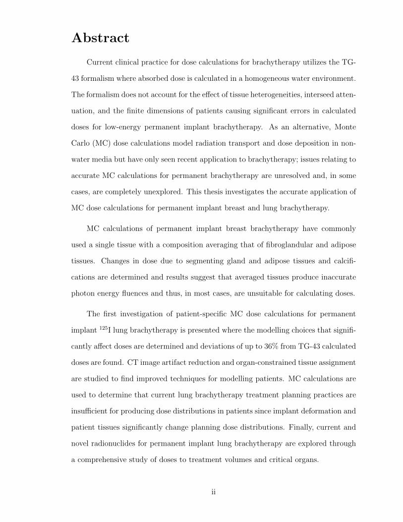
Abstract
Current clinical practice for dose calculations for brachytherapy utilizes the TG-
43 formalism where absorbed dose is calculated in a homogeneous water environment.
The formalism does not account for the effect of tissue heterogeneities, interseed atten-
uation, and the finite dimensions of patients causing significant errors in calculated
doses for low-energy permanent implant brachytherapy. As an alternative, Monte
Carlo (MC) dose calculations model radiation transport and dose deposition in non-
water media but have only seen recent application to brachytherapy; issues relating to
accurate MC calculations for permanent brachytherapy are unresolved and, in some
cases, are completely unexplored. This thesis investigates the accurate application of
MC dose calculations for permanent implant breast and lung brachytherapy.
MC calculations of permanent implant breast brachytherapy have commonly
used a single tissue with a composition averaging that of fibroglandular and adipose
tissues. Changes in dose due to segmenting gland and adipose tissues and calcifi-
cations are determined and results suggest that averaged tissues produce inaccurate
photon energy fluences and thus, in most cases, are unsuitable for calculating doses.
The first investigation of patient-specific MC dose calculations for permanent
implant 125I lung brachytherapy is presented where the modelling choices that signifi-
cantly affect doses are determined and deviations of up to 36% from TG-43 calculated
doses are found. CT image artifact reduction and organ-constrained tissue assignment
are studied to find improved techniques for modelling patients. MC calculations are
used to determine that current lung brachytherapy treatment planning practices are
insufficient for producing dose distributions in patients since implant deformation and
patient tissues significantly change planning dose distributions. Finally, current and
novel radionuclides for permanent implant lung brachytherapy are explored through
a comprehensive study of doses to treatment volumes and critical organs.
ii
Acknowledgments
I would like to express my sincere gratitude towards my supervisors, Dr. Rowan
Thomson and Dr. Dave Rogers. Together, they have provided me with immeasurable
guidance, direction, and expertise. Dave sets a high standard of excellence that
will surely affect me throughout my future endeavours. Additionally, his open-door
policy and cheerful insights have always been greatly appreciated. Rowan’s tireless
involvement with the work of her students shows in her enthusiasm and willingness
to always provide valuable guidance. The decision for Rowan to be my co-supervisor
when she became a faculty member was easily one of the most advantageous events
of my time at Carleton. I hope that she considers taking me on as her first student
to be a fraction as positive a milestone as being her student has been for me.
I would like to thank Dr. Keith Furutani of the Mayo Clinic for his highly
important insights and perspective on our collaborative work. The majority of this
thesis would not have been possible without him. I would also like to thank a number
of my colleagues at Carleton including Bryan Muir, Nelson Miksys, Elsayed Ali,
Marielle Lesperance, Martin Martinov, and Manuel Rodriguez for their help and
friendship.
I’m always deeply grateful to my parents for their love and support. Their
encouragement and enthusiasm for my achievemen ts have been invaluable. To my
wife, Becky: thank you for your support, love, encouragement, and most importantly
your patience! You’ve always been there for me and I can’t thank you enough for the
irreplaceable role you’ve played in my life. Finally, I want to thank my one-year-old
son, Owen, for the endless joy he’s added to our lives.
This work has been supported by an Ontario Graduate Scholarship in science
and technology, an Ontario Graduate Scholarship, as well as the Kiwanis Club of
Ottawa Medical Foundation and Dr. Kanta Marwah Scholarship in Medical Physics.
iii
Statement of originality
This thesis is a summary of the most significant portion of the author’s work
during the course of his Ph.D. program at Carleton University. It is based on the
journal papers listed below. Most of the results have or will also be presented at
national and international conferences.
Dr. Dave Rogers and Dr. Rowan Thomson supervised the project and provided
input on all of its components, including the publications. Otherwise, the author of
this thesis performed all of the computational work, and drafted and revised all of
the manuscripts. A description of where the results of each publication can be found
in the thesis is given below.
Peer-reviewed papers
I. J. G. H. Sutherland and D. W. O. Rogers, “Monte Carlo calculated absorbed-dose
energy dependence of EBT and EBT2 film”, Med. Phys. 37, 1110 – 1116 (2010).
• The results of this paper are unrelated to the topic of the thesis and are not
included. The paper is listed to provide a complete view of the author’s publi-
cations.
II. J. G. H. Sutherland, R. M. Thomson, and D. W. O. Rogers, “Changes in dose with
segmentation of breast tissues in Monte Carlo calculations for low-energy brachyther-
apy”, Med. Phys. 38, 4858 – 4865 (2011).
• The results of this paper appear in chapter 3 when discussing segmentation of
breast tissues for Monte Carlo calculations of low-energy brachytherapy.
• The results of this paper were presented as a poster at the Joint AAPM/COMP
Meeting in Vancouver, BC (2011).
iv
III. J. G. H. Sutherland, K. M. Furutani, Y. I. Garces, and R. M. Thomson, “Model-
based dose calculations for 125I lung brachytherapy”, Med. Phys. 39, 4365 – 4377 (2012).
• The results of this paper appear in chapter 4 when discussing Monte Carlo
calculations for 125I lung brachytherapy.
• The results of this paper were presented as an oral presentation at the Joint
AAPM/COMP Meeting in Vancouver, BC (2011).
IV. J. G. H. Sutherland, K. M. Furutani, and R. M. Thomson, “A Monte Carlo
investigation of lung brachytherapy treatment planning”, Phys. Med. Biol., 58, 4763 –
4780 (2013).
• The results of this paper appear in chapter 6 when discussing a Monte Carlo
investigation of lung brachytherapy treatment planning.
• The results of this paper were presented as an oral presentation at the COMP
Annual Scientific Meeting in Halifax, NS (2012).
V. J. G. H. Sutherland, N. Miksys, K. M. Furutani, and R. M. Thomson, “Metallic
artifact mitigation and organ-constrained tissue assignment for Monte Carlo calcula-
tions of lung brachytherapy”, Med. Phys., submitted.
• The results of this paper appear in chapter 5 when discussing the comparison of
metallic artifact reduction techniques and organ-constrained tissue assignments
for Monte Carlo of permanent implant lung brachytherapy.
• The results of this paper were presented as an oral presentation at the AAPM
Annual Meeting & Exhibition in Indianapolis, IN (2013).
VI. J. G. H. Sutherland, K. M. Furutani, and R. M. Thomson, “Monte Carlo cal-
culated doses to treatment volumes and organs at risk for lung brachytherapy”,
Phys. Med. Biol., submitted.
• The results of this paper appear in chapter 7 when discussing the Monte Carlo
calculated doses to treatment volumes and organs at risk using various radionu-
clides for permanent implant lung brachytherapy.
• The results of this paper will be presented as a poster at the CARO-COMP
Joint Scientific Meeting in Montreal QC (2013).
v
Contents
Abstract i
Acknowledgements iii
Statement of originality iv
Contents vi
List of Tables x
List of Figures xii
1 Introduction 1
1.1 Brachytherapy . . . . . . . . . . . . . . . . . . . . . . . . . . . . . . . 2
1.1.1 Permanent breast seed implant brachytherapy (PBSI) . . . . . 2
1.1.2 Intraoperative brachytherapy for stage I non-small cell lung car-
cinoma . . . . . . . . . . . . . . . . . . . . . . . . . . . . . . . 4
1.2 Current clinical brachytherapy dosimetry practice: TG-43 . . . . . . 5
1.3 Model-based dose calculations for brachytherapy . . . . . . . . . . . . 7
1.4 Monte Carlo simulations . . . . . . . . . . . . . . . . . . . . . . . . . 8
1.5 Outline of thesis . . . . . . . . . . . . . . . . . . . . . . . . . . . . . . 11
2 Model-based dose calculations for brachytherapy 13
vi
2.1 EGSnrc . . . . . . . . . . . . . . . . . . . . . . . . . . . . . . . . . . 13
2.2 BrachyDose . . . . . . . . . . . . . . . . . . . . . . . . . . . . . . . . 14
2.3 Calculating absolute dose . . . . . . . . . . . . . . . . . . . . . . . . . 15
2.4 Using patient data for BrachyDose calculations . . . . . . . . . . . . 17
2.4.1 Elemental composition of voxels . . . . . . . . . . . . . . . . . 18
2.4.2 Tools for files in DICOM format . . . . . . . . . . . . . . . . . 18
2.5 Simulation parameters . . . . . . . . . . . . . . . . . . . . . . . . . . 21
3 Breast tissue segmentation 22
3.1 Methods . . . . . . . . . . . . . . . . . . . . . . . . . . . . . . . . . . 23
3.1.1 Dose to gland and adipose versus dose to an averaged tissue . 25
3.1.2 Effect of realistic segmentation on photon energy
fluence . . . . . . . . . . . . . . . . . . . . . . . . . . . . . . . 27
3.1.3 The effect of calcifications on photon energy fluence . . . . . . 28
3.2 Results and Discussion . . . . . . . . . . . . . . . . . . . . . . . . . . 29
3.2.1 Dose to gland and adipose versus dose to an averaged tissue . 29
3.2.2 Realistic segmentation and its effect on photon energy fluence 32
3.2.3 The effect of calcifications . . . . . . . . . . . . . . . . . . . . 37
3.3 Conclusions . . . . . . . . . . . . . . . . . . . . . . . . . . . . . . . . 40
4 Exploring model-based dose calculations for 125I lung brachytherapy 43
4.1 Methods . . . . . . . . . . . . . . . . . . . . . . . . . . . . . . . . . . 45
4.1.1 Correcting metallic artifacts . . . . . . . . . . . . . . . . . . . 46
4.1.2 Tissue assignment schemes . . . . . . . . . . . . . . . . . . . . 50
4.1.3 Comparison with TG-43 . . . . . . . . . . . . . . . . . . . . . 54
4.2 Results . . . . . . . . . . . . . . . . . . . . . . . . . . . . . . . . . . . 55
vii
4.2.1 Correcting metallic artifacts . . . . . . . . . . . . . . . . . . . 55
4.2.2 Tissue assignment schemes . . . . . . . . . . . . . . . . . . . . 59
4.2.3 Comparison with TG-43 . . . . . . . . . . . . . . . . . . . . . 62
4.3 Discussion . . . . . . . . . . . . . . . . . . . . . . . . . . . . . . . . . 65
4.4 Conclusions . . . . . . . . . . . . . . . . . . . . . . . . . . . . . . . . 70
5 Metallic artifact mitigation and organ-constrained tissue assignment
for lung brachytherapy 72
5.1 Methods . . . . . . . . . . . . . . . . . . . . . . . . . . . . . . . . . . 74
5.1.1 Metallic artifact reduction . . . . . . . . . . . . . . . . . . . . 74
5.1.2 Tissue assignment schemes and development of computational
phantoms . . . . . . . . . . . . . . . . . . . . . . . . . . . . . 75
5.2 Results and Discussion . . . . . . . . . . . . . . . . . . . . . . . . . . 78
5.2.1 Metallic artifact reduction . . . . . . . . . . . . . . . . . . . . 78
5.2.2 Tissue assignment schemes and dose . . . . . . . . . . . . . . 83
5.3 Conclusions . . . . . . . . . . . . . . . . . . . . . . . . . . . . . . . . 91
6 A Monte Carlo investigation of lung brachytherapy treatment plan-
ning 95
6.1 Methods . . . . . . . . . . . . . . . . . . . . . . . . . . . . . . . . . . 96
6.1.1 Effect of non-water media on prescription dose . . . . . . . . . 97
6.1.2 Effect of seed grid deformation and patient-defined media . . . 99
6.2 Results and discussion . . . . . . . . . . . . . . . . . . . . . . . . . . 103
6.2.1 Effect of non-water media on prescription dose . . . . . . . . . 103
6.2.2 Effect of seed grid deformation and patient-defined media . . . 109
6.3 Conclusions . . . . . . . . . . . . . . . . . . . . . . . . . . . . . . . . 114
viii
7 Monte Carlo calculated doses to treatment volumes and organs at
risk for permanent implant lung brachytherapy 117
7.1 Methods . . . . . . . . . . . . . . . . . . . . . . . . . . . . . . . . . . 119
7.2 Results and Discussion . . . . . . . . . . . . . . . . . . . . . . . . . . 124
7.2.1 Doses to treatment volumes . . . . . . . . . . . . . . . . . . . 124
7.2.2 Doses to the right lung . . . . . . . . . . . . . . . . . . . . . . 130
7.2.3 Doses to the aorta . . . . . . . . . . . . . . . . . . . . . . . . 134
7.2.4 Doses to the heart . . . . . . . . . . . . . . . . . . . . . . . . 138
7.3 Conclusions . . . . . . . . . . . . . . . . . . . . . . . . . . . . . . . . 140
8 Conclusions 142
8.1 Overview . . . . . . . . . . . . . . . . . . . . . . . . . . . . . . . . . . 142
8.2 Summary of conclusions . . . . . . . . . . . . . . . . . . . . . . . . . 143
8.3 Impact and future work . . . . . . . . . . . . . . . . . . . . . . . . . 145
References 147
ix
List of Tables
2.1 Composition of tissues used in calculations . . . . . . . . . . . . . . . 19
4.1 Mass attenuation and energy absorption coefficients for 28 keV photons 51
4.2 CT number / mass density calibration data . . . . . . . . . . . . . . 52
4.3 Dose metrics of lung brachytherapy patients for artifact corr. methods 59
4.4 Dose metrics of lung brachytherapy patients for tissue assign. schemes 61
4.5 Dose metrics of lung brachytherapy patients using TG-43 and MBDCs 65
5.1 Summary of metallic artifact reduction techniques . . . . . . . . . . . 76
5.2 Dose metrics for various phantoms of lung brachytherapy patient 1 . 84
5.3 Dose metrics for various phantoms of lung brachytherapy patient 2 . 85
5.4 Dose metrics for various phantoms of lung brachytherapy patient 5 . 86
5.5 Percentage of voxels assigned to bone for phantoms . . . . . . . . . . 87
6.1 Mass attenuation and energy absorption coefficients for 28 and 30 keV
photons . . . . . . . . . . . . . . . . . . . . . . . . . . . . . . . . . . 97
6.2 Lung brachytherapy treatment planning nomogram seed configurations 98
6.3 Notation and description of dose calculation for prescription dose analysis 99
6.4 Monte Carlo calculated nomograms for TG-43point and Dl,l(0.26) . . . . 108
6.5 V100 for PTV05 and PTV20 for virtual implants . . . . . . . . . . . . 111
6.6 D90 for PTV05 and PTV20 for virtual implants . . . . . . . . . . . . 112
x
7.1 Mass attenuation and energy absorption coefficient ratios of water to
tissues . . . . . . . . . . . . . . . . . . . . . . . . . . . . . . . . . . . 120
7.2 Mean and standard deviations of D90 . . . . . . . . . . . . . . . . . . 125
7.3 Mean and standard deviations of V100 and V200 . . . . . . . . . . . . 128
7.4 Mean dose to lung for fissure implant . . . . . . . . . . . . . . . . . . 132
xi
List of Figures
1.1 Diagram of PBSI implant procedure . . . . . . . . . . . . . . . . . . . 3
1.2 Diagram of lung brachytherapy procedure . . . . . . . . . . . . . . . 5
1.3 Diagram of TG-43 coordinate system . . . . . . . . . . . . . . . . . . 7
1.4 Mass attenuation and energy absorption ratios . . . . . . . . . . . . . 9
2.1 Diagram depicting calculation of dose to a fictitious voxel medium . . 17
3.1 Diagrams of various breast phantoms . . . . . . . . . . . . . . . . . . 26
3.2 DVHs for dose to gland in averaged tissue and randomly segmented
phantoms . . . . . . . . . . . . . . . . . . . . . . . . . . . . . . . . . 30
3.3 DVHs for entire phantoms in averaged tissue and randomly segmented
phantoms . . . . . . . . . . . . . . . . . . . . . . . . . . . . . . . . . 31
3.4 Dose profiles for various breast phantoms . . . . . . . . . . . . . . . . 32
3.5 DVHs for dose to various tissues in realistically segmented and averaged
tissue phantoms . . . . . . . . . . . . . . . . . . . . . . . . . . . . . . 33
3.6 DVHs for entire phantoms for realistically segmented and averaged
tissue phantoms . . . . . . . . . . . . . . . . . . . . . . . . . . . . . . 35
3.7 DVHs for dose to gland voxels in phantoms with calcification . . . . . 38
3.8 DVHs for entire phantoms for phantoms with calcification . . . . . . 39
3.9 DVHs for dose to non-calcification media for phantoms with calcification 41
xii
4.1 CT profiles for uncorrected and vsMAR corrected data for a lung
brachytherapy patient . . . . . . . . . . . . . . . . . . . . . . . . . . 48
4.2 A portion of a CT image showing artifact reduction methods . . . . . 49
4.3 Histogram showing the frequency of CT numbers in several lung brachyther-
apy patient CT phantoms . . . . . . . . . . . . . . . . . . . . . . . . 52
4.4 Tissue assignment schemes . . . . . . . . . . . . . . . . . . . . . . . . 54
4.5 Dose profiles showing results of artifact reduction in a lung brachyther-
apy patient . . . . . . . . . . . . . . . . . . . . . . . . . . . . . . . . 56
4.6 CT image showing line used for profile in figure 4.5 . . . . . . . . . . 56
4.7 DVHs showing result of metallic artifact reduction in a lung brachyther-
apy patient . . . . . . . . . . . . . . . . . . . . . . . . . . . . . . . . 60
4.8 DVHs showing result of tissue assignment schemes in a lung brachyther-
apy patient . . . . . . . . . . . . . . . . . . . . . . . . . . . . . . . . 62
4.9 Dose profile showing result of tissue assignment schemes in a lung
brachytherapy patient . . . . . . . . . . . . . . . . . . . . . . . . . . 63
4.10 CT image showing the line used for the dose profile in figure 4.9 . . . 63
4.11 DVHs comparing TG-43 and MBDCs for two lung brachytherapy patients 66
4.12 Dose profiles comparing TG-43 and MBDCs for a lung brachytherapy
patient . . . . . . . . . . . . . . . . . . . . . . . . . . . . . . . . . . . 67
5.1 Diagram showing constrained and unconstrained tissue assign. schemes 77
5.2 Uncorrected CT image for a lung brachytherapy patient . . . . . . . . 78
5.3 CT images and difference images after application of artifact reduction 79
5.4 CT number profiles for artifact reduced CT images . . . . . . . . . . 82
5.5 Dose profiles for phantoms of lung brachytherapy patient 2 . . . . . . 89
5.6 Dose and density profiles illustrating effect of using nominal tissue
densities . . . . . . . . . . . . . . . . . . . . . . . . . . . . . . . . . . 91
xiii
5.7 Composite dose and density distributions showing profile lines for fig-
ure 5.6 . . . . . . . . . . . . . . . . . . . . . . . . . . . . . . . . . . . 92
6.1 Diagram showing nomogram seed configurations B and D . . . . . . . 98
6.2 Illustration showing the 5 virtual implants and contours of right lung 100
6.3 Illustration of the virtual implant creation algorithm . . . . . . . . . 101
6.4 Normalized prescription doses for different dose calculations . . . . . 104
6.5 Isodose contours comparing TG-43sim to Dl,l(0.26) for planning seed con-
figuration . . . . . . . . . . . . . . . . . . . . . . . . . . . . . . . . . 106
6.6 Normalized Dl,l(0.26) prescription doses for different seed configurations 107
6.7 TG-43sim DVHs for PTV05s illustrating effects of deformation . . . . 109
6.8 DVHs for PTV05 of “fissure” virtual implant . . . . . . . . . . . . . . 112
6.9 DVHs for PTV05 and PTV20 of “superior” virtual implant . . . . . . 113
6.10 Dose and density profiles for “superior” virtual implant . . . . . . . . 115
7.1 Diagram of tissue assignment scheme for lung doses . . . . . . . . . . 121
7.2 CT image with heart and aorta contours and centres of implants . . . 122
7.3 Illustration of virtual implant no. 1 . . . . . . . . . . . . . . . . . . . 123
7.4 D90 for treatment volumes for source types . . . . . . . . . . . . . . . 126
7.5 V100 for treatment volumes for source types . . . . . . . . . . . . . . 129
7.6 Mean dose to lung for implants . . . . . . . . . . . . . . . . . . . . . 131
7.7 DVH of dose to lung for fissure implant . . . . . . . . . . . . . . . . . 133
7.8 Mean dose to the aorta . . . . . . . . . . . . . . . . . . . . . . . . . . 135
7.9 V5 of the heart for implants . . . . . . . . . . . . . . . . . . . . . . . 137
7.10 Mean dose to the heart for implants . . . . . . . . . . . . . . . . . . . 139
xiv

Chapter 1
Introduction
According to the Canadian Cancer Society, approximately 40% of Canadians will
develop cancer in their lifetimes and 25% will die of the disease1. Common cancer
treatments are surgery, chemotherapy, immunotherapy, monoclonal antibodies, and
radiation therapy. Radiation therapy is the medical use of ionizing radiation to con-
trol malignant tumour cells. Often used in concert with surgery and/or chemotherapy
both curatively and palliatively, the objective of radiation therapy is to destroy ma-
lignant cells by damaging their genetic material while simultaneously sparing as much
healthy tissue as possible.
The three principal modes of radiation therapy are systemic radiation therapy,
external beam radiation therapy, and brachytherapy2. Systemic radiation therapy
targets cancer cells by injecting a liquid radiation source into the body. External
beam radiation therapy directs radiation at a patient’s body from an external ma-
chine. Common sources for external beam radiation therapy are γ rays produced by
radionuclides such as 60Co and x rays, electrons, and heavier charged particles such
as protons produced by linear accelerators (linacs)3. Brachytherapy, the focus of this
thesis, is described in the following section.
1
2
1.1 Brachytherapy
Brachytherapy is a form of radiation therapy where a radiation source is placed next
to or inside a treatment site and is used as a treatment for cervical, prostate, skin,
ocular, breast and lung cancers among other sites. Brachytherapy treatments are
commonly divided into two forms (see eg. Podgorsak et al.4). In high-dose rate
(HDR) brachytherapy, the rate of dose delivery is greater than 12 Gy·h−1 and single
sources (commonly 192Ir) are delivered to the treatment site for a short period of
time using catheters and a remote afterloader. Low-dose rate (LDR) treatments have
numerous encapsulated sources or seeds (approximately the size of a grain of rice)
that emit at a rate of 2 Gy·h−1 or less to a treatment-site-specific reference point and
are surgically implanted either permanently or are removed after several days.
The use of low energy (. 50 keV) radionuclides for permanent implant LDR
brachytherapy began in the late 1960s with 125I seeds5, followed by the adoption of
103Pd and later 131Cs. The ease of manipulating and disposing of these seeds makes
them attractive sources and their use has revolutionized the practice of permanent
implantation. The most common use of these low energy seeds is permanent seed
implantation for the treatment of early stage prostate carcinoma, but permanent
seed implantation treatments have also been more recently developed as adjuvant
radiation treatments for early stage breast cancer6,7 and stage I non-small cell lung
cancer8,9 which are of particular interest in this thesis.
1.1.1 Permanent breast seed implant brachytherapy (PBSI)
While breast cancer is the most commonly diagnosed cancer in women, the majority
of women are diagnosed with early-stage, localized disease due to widespread screen-
1.1. BRACHYTHERAPY
3
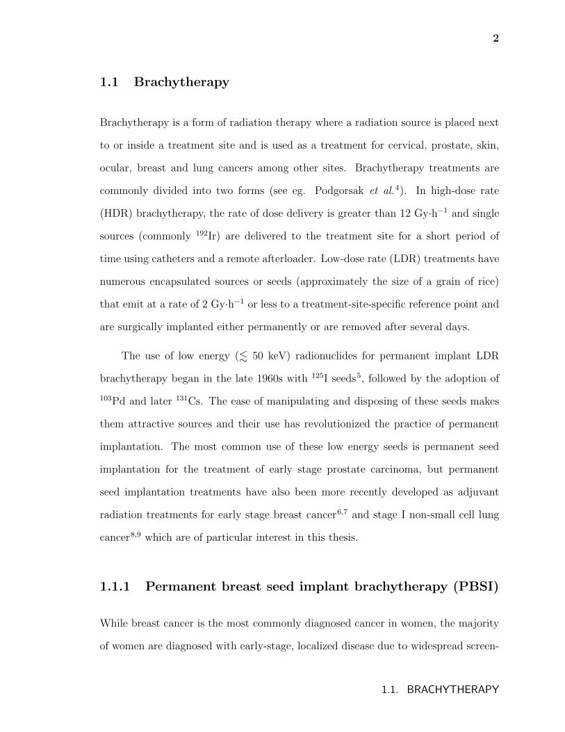
Figure 1.1: Diagram showing permanent breast seed implant procedure
ing mammography. Pignol et al.6 developed a permanent seed implant treatment as
an alternative to the standard breast radiation in which high-energy x rays are deliv-
ered over a period of 3.5 to 7 weeks10. With its highly localized dose distributions,
brachytherapy is an attractive treatment for early stage cancer.
In this technique6, eligible patients with early-stage breast cancer that have
received breast-conserving surgery are imaged with breast ultrasound (US) to localize
and measure the size of the surgical bed. Computed tomography (CT) imaging is
performed so that target volumes and seed placement planning can be performed in
a treatment planning system (TPS). A dose of 90 Gy is prescribed to the minimal
peripheral dose that covers planning treatment volumes using 103Pd seeds spaced 1 cm
apart in a volume. Seeds are implanted in anesthetized patients using a fiducial needle
under ultrasound guidance with the help of a needle spacing template immobilized
by a mechanical arm (see figure 1.1). CT images acquired 2 months post-implant are
used to identify seed positions and perform quality assurance.
1.1. BRACHYTHERAPY
4
1.1.2 Intraoperative brachytherapy for stage I non-small cell
lung carcinoma
In both Canada and the U.S., lung cancer is the leading cause of cancer death11,12.
While the standard treatment for stage I non-small cell lung cancer is lobectomy
(i.e., the removal of an entire lobe of the lung) for many patients this treatment
poses too great a risk due to poor pulmonary reserve and so sublobar resection (i.e.,
the removal of only the tumour plus a margin) is used13. Unfortunately, limited
resections have been associated with a larger incidence of local recurrence14. External
beam radiotherapy can be used to reduce the higher rate of local recurrence associated
with sublobar resection compared to lobectomy, but this can also increase morbidity
due to cardiac toxicity, lung fibrosis, and loss of pulmonary function15.
In recent years, 125I brachytherapy has been used in conjunction with sublobar
resection to treat stage I non-small cell lung cancer and has been reported to improve
disease-free and overall survival rates compared with resection alone.8,9,15–20 In fact,
the use of 125I brachytherapy has been reported to reduce local recurrence of cancer
after sublobar resection from 18.6% to 2% (Ref. 17) and elsewhere has been described
as being a conformal radiation therapy without the concerns of treatment errors due
to breathing15. While the majority of treatments are performed using 125I seeds, the
use of additional radionuclides such as 131Cs (Ref. 21) and 169Yb (Ref. 22) are also
under investigation.
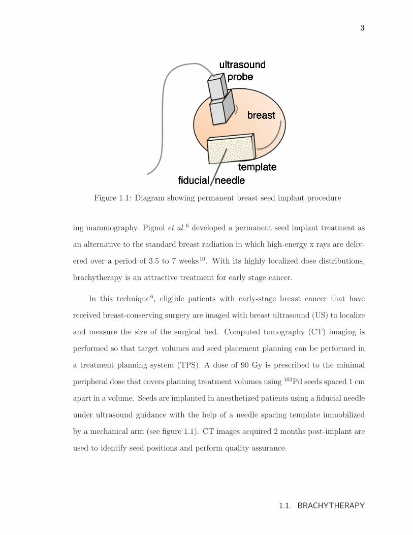
In one brachytherapy technique23, an implant is created during the surgical pro-
cedure by weaving strands of 125I seeds into a vicryl mesh which is then sutured over
the resection staple line with the goal of delivering 100 Gy at 5 to 7 mm along the
central axis of the resection margin (see fig. 1.2). Post-treatment CT images are used
to identify seed positions and contour suture lines and volumes of interest.
1.1. BRACHYTHERAPY
5
Figure 1.2: Diagram showing lung brachytherapy implant procedure
1.2 Current clinical brachytherapy dosimetry practice: TG-43
Dosimetry is the practice of calculating or measuring absorbed-dose (i.e., energy ab-
sorbed per unit mass) due to radiation in some medium. In brachytherapy, dosimetry
calculation practices are used to determine the distribution of sources in defined vol-
umes to achieve clinically acceptable dose distributions, calculate patient doses, and
provide a system for dose prescription24.
The current clinical approach for brachytherapy dose calculation is performed us-
ing the formalism described by the recommendations of the AAPM Radiation Ther-
apy Committee Task Group No. 43 (TG-43)25–27. The TG-43 formalism uses an
analytic expression to calculate the dose in a homogeneous, liquid water environment
at any point surrounding a single brachytherapy seed. The expression uses a polar
coordinate system along the long axis of sources that are assumed to be cylindri-
cally symmetric. Parameters of the expression are either determined experimentally
or using Monte Carlo methods. Dose distributions for implants with multiple seeds
are calculated by summing the contribution from each seed individually and, conse-
1.2. CURRENT CLINICAL BRACHYTHERAPY DOSIMETRY PRACTICE: TG-43
6
quently, this approach does not account for the effect that attenuation and scatter of
each seed would have on the dose distributions of other seeds.
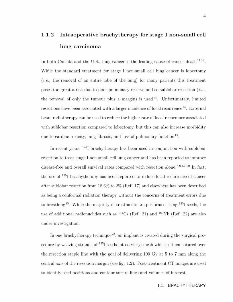
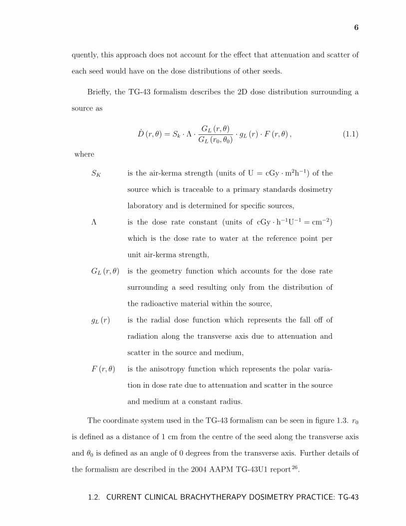
Briefly, the TG-43 formalism describes the 2D dose distribution surrounding a
source as
D (r, θ) = Sk · Λ · GL (r, θ)
GL (r0, θ0)· gL (r) · F (r, θ) , (1.1)
where
SK is the air-kerma strength (units of U = cGy · m2h−1) of the
source which is traceable to a primary standards dosimetry
laboratory and is determined for specific sources,
Λ is the dose rate constant (units of cGy · h−1U−1 = cm−2)
which is the dose rate to water at the reference point per
unit air-kerma strength,
GL (r, θ) is the geometry function which accounts for the dose rate
surrounding a seed resulting only from the distribution of
the radioactive material within the source,
gL (r) is the radial dose function which represents the fall off of
radiation along the transverse axis due to attenuation and
scatter in the source and medium,
F (r, θ) is the anisotropy function which represents the polar varia-
tion in dose rate due to attenuation and scatter in the source
and medium at a constant radius.
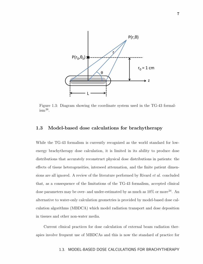
The coordinate system used in the TG-43 formalism can be seen in figure 1.3. r0
is defined as a distance of 1 cm from the centre of the seed along the transverse axis
and θ0 is defined as an angle of 0 degrees from the transverse axis. Further details of
the formalism are described in the 2004 AAPM TG-43U1 report26.
1.2. CURRENT CLINICAL BRACHYTHERAPY DOSIMETRY PRACTICE: TG-43
7
P(r0,θ0)(
P(r,θ)(
z(
r0 =(1(cm(
L(
r(
θ(
Figure 1.3: Diagram showing the coordinate system used in the TG-43 formal-ism26.
1.3 Model-based dose calculations for brachytherapy
While the TG-43 formalism is currently recognized as the world standard for low-
energy brachytherapy dose calculation, it is limited in its ability to produce dose
distributions that accurately reconstruct physical dose distributions in patients: the
effects of tissue heterogeneities, interseed attenuation, and the finite patient dimen-
sions are all ignored. A review of the literature performed by Rivard et al. concluded
that, as a consequence of the limitations of the TG-43 formalism, accepted clinical
dose parameters may be over- and under-estimated by as much as 10% or more24. An
alternative to water-only calculation geometries is provided by model-based dose cal-
culation algorithms (MBDCA) which model radiation transport and dose deposition
in tissues and other non-water media.
Current clinical practices for dose calculation of external beam radiation ther-
apies involve frequent use of MBDCAs and this is now the standard of practice for
1.3. MODEL-BASED DOSE CALCULATIONS FOR BRACHYTHERAPY
8
modalities such as intensity modulated radiation therapy (IMRT)28. This contrasts
the relatively rare use of MBDCAs in the brachytherapy community, where het-
erogeneity correction algorithms and other MBDCAs have only recently been made
available24,29.
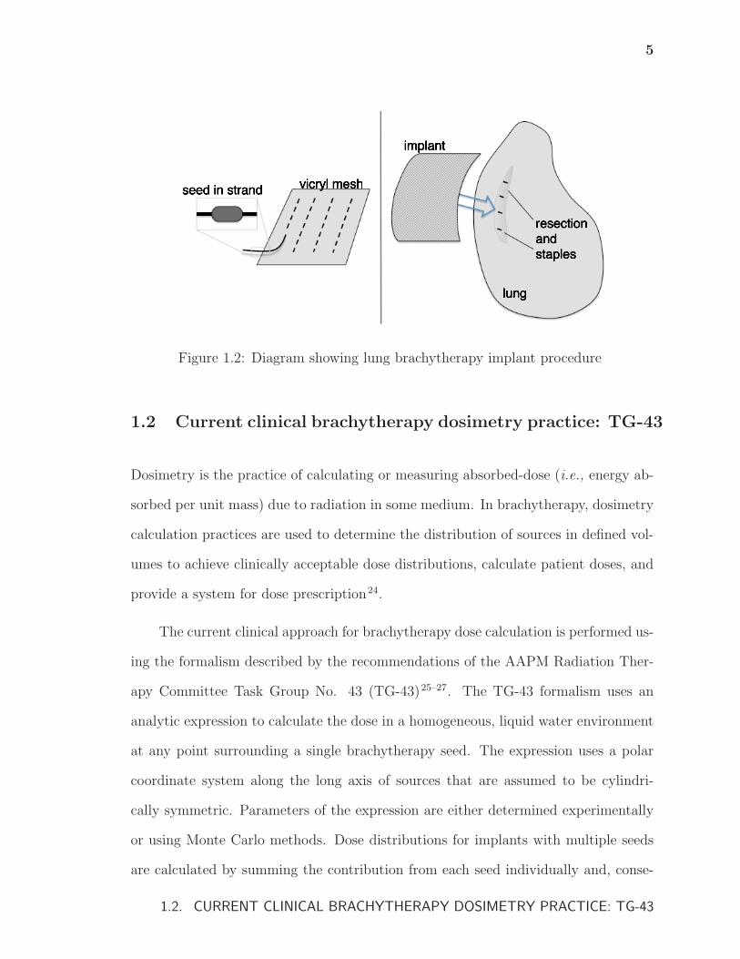
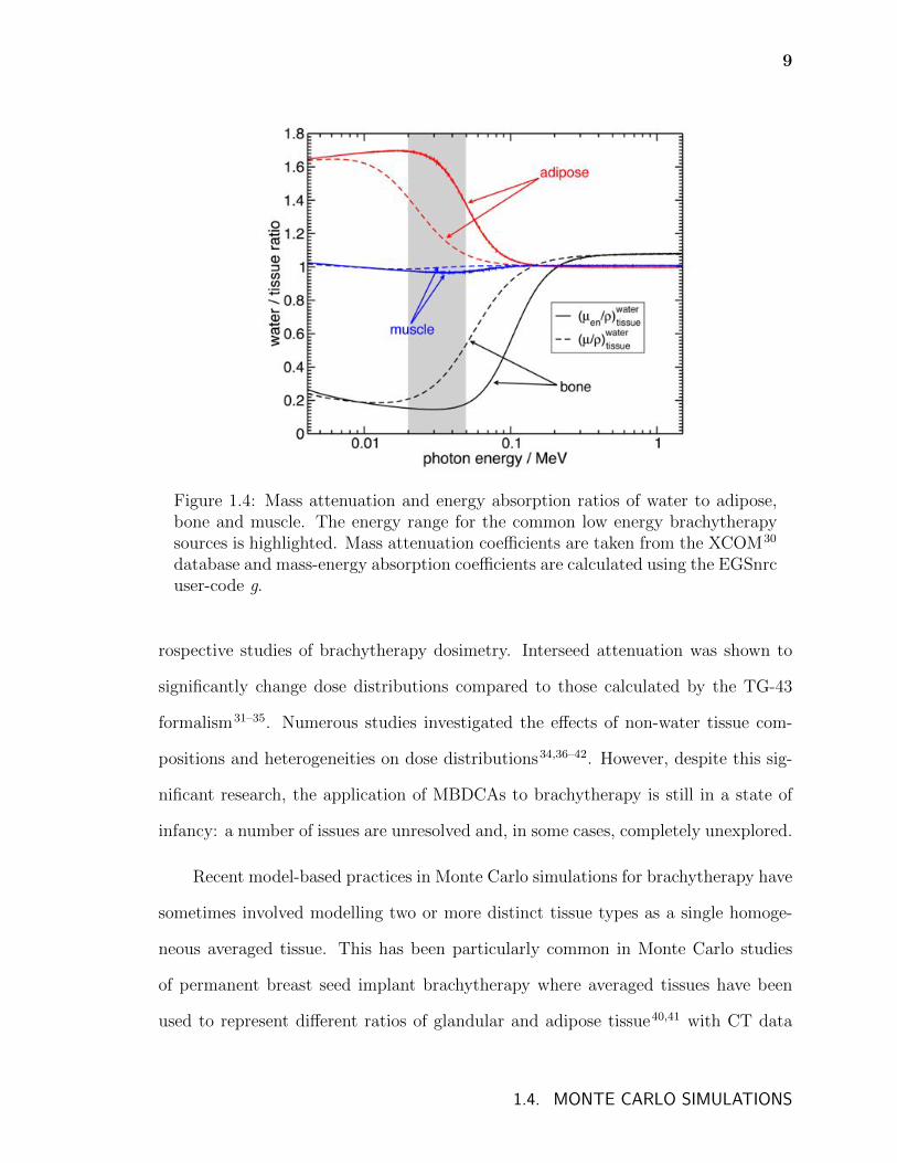
Photon interaction processes in the energy range of external beam radiation
therapy are dominated by Compton scattering while those for the photon energies of
low energy brachytherapy are dominated by the photoelectric effect. Consequently,
the differences in the attenuation and scatter of photons and absorbed dose between
water and non-water media will be significantly more dramatic for brachytherapy
dose calculations. This is illustrated in figure 1.4 which shows the mass attenuation
and energy absorption ratios of water to adipose, bone, and muscle as a function of
photon energy. The energy range for the common low energy brachytherapy sources
is highlighted.
The inability of the water-based TG-43 approach to accurately calculate dose
distributions in patient geometries underlines the need for accurate model-based dose
calculations for low-energy permanent implant brachytherapy.
1.4 Monte Carlo simulations
The Monte Carlo (MC) method of dose calculation, considered to be the current
state of the art in computational dosimetry, is based on the sampling of known prob-
ability distributions to simulate trajectories and interactions of particle histories to
estimate absorbed dose. Consequently, it has the ability to account for interseed ef-
fects, calculate absorbed dose to tissue rather than water, simulate dose calculations
in heterogeneous media, and to model patient specific geometries.
Recently, Monte Carlo methods have been used to perform explorative and ret-
1.4. MONTE CARLO SIMULATIONS
9
Figure 1.4: Mass attenuation and energy absorption ratios of water to adipose,bone and muscle. The energy range for the common low energy brachytherapysources is highlighted. Mass attenuation coefficients are taken from the XCOM30
database and mass-energy absorption coefficients are calculated using the EGSnrcuser-code g.
rospective studies of brachytherapy dosimetry. Interseed attenuation was shown to
significantly change dose distributions compared to those calculated by the TG-43
formalism31–35. Numerous studies investigated the effects of non-water tissue com-
positions and heterogeneities on dose distributions34,36–42. However, despite this sig-
nificant research, the application of MBDCAs to brachytherapy is still in a state of
infancy: a number of issues are unresolved and, in some cases, completely unexplored.
Recent model-based practices in Monte Carlo simulations for brachytherapy have
sometimes involved modelling two or more distinct tissue types as a single homoge-
neous averaged tissue. This has been particularly common in Monte Carlo studies
of permanent breast seed implant brachytherapy where averaged tissues have been
used to represent different ratios of glandular and adipose tissue40,41 with CT data
1.4. MONTE CARLO SIMULATIONS
10
sometimes being used to assign the mass density to each voxel41. The question of
the accuracy of using homogeneous averaged tissues in breast calculations (and for
low energy brachytherapy in general) and under which conditions their use might be
justified in lieu of fully segmented phantoms has not been thoroughly investigated.
Additionally, the modelling of calcifications in breast and prostate patient geometries
has only seen preliminary treatment in the literature37,43.
Patient specific MBDCs generally require that interaction cross sections be as-
signed on a voxel-by-voxel basis. CT imaging is the standard for fulfilling this need,
but unfortunately, provides only voxel electron density which does not relate directly
to elemental composition and density. While the assignment of tissues of distinct
atomic composition to voxels based on CT number has been investigated in the con-
text of external beam radiation therapy44–47, very little focus has been made on the
dosimetric results of this practice for the energy ranges of interest in brachyther-
apy48. Additionally, the presence of metallic brachytherapy seeds in CT images cre-
ates streaking artifacts and while the correction of these artifacts has been an active
area of research49–52, changes in brachytherapy dose distributions as a result of these
considerations have not been reported.
Finally, in contrast to prostate33–35,37,42, breast40–42,53 and occular38,39,54 low en-
ergy brachytherapy treatments, intraoperative lung brachytherapy has been almost
entirely neglected by the MBDCA research community with only one preliminary
investigation reported55. Considering the highly heterogeneous treatment sites of
lung brachytherapy, the differences between Monte Carlo and TG-43 calculated dose
distributions have the potential to be dramatic for these treatments.
1.4. MONTE CARLO SIMULATIONS
11
1.5 Outline of thesis
The chapters that follow investigate the accurate application of Monte Carlo dose
calculations to permanent implant breast and lung brachytherapy. The importance
of segmenting tissues in Monte Carlo phantom models is explored. The use of patient
CT images for calculating patient specific dose distributions and the challenges that
need to be overcome in doing so are presented. Finally, Monte Carlo calculations
are used to further the understanding of treatment planning and patient doses for
permanent implant lung brachytherapy.
Chapter 2 introduces the EGSnrc Monte Carlo user code BrachyDose used through-
out this thesis and then describes the code and methodologies used in this work to
produce patient-specific model-based dose calculations.
Chapter 3 begins with a brief review of the literature concerning the application
of Monte Carlo dose calculations to permanent breast seed implant brachytherapy and
then presents an investigation into the changes of dose due to segmentation of breast
tissues. Dose distributions in phantom models with segmented adipose and glandular
tissues are compared with those of phantoms consisting of a single averaged tissue.
This chapter also investigates the method commonly used in mammography radiation
protection calculations to estimate the average dose to glandular tissue by using non-
segmented computational phantoms. Finally, the effect of breast calcifications and
the impact that their presence have on the need to segment breast tissues is presented.
Chapter 4 presents the first investigation of patient specific Monte Carlo dose
calculations for 125I lung brachytherapy and identifies some of the significant modelling
challenges of using CT data to produce computational phantoms. The final effects
on dose distributions of metallic artifact correction methods for mitigating streaking
1.5. OUTLINE OF THESIS
12
artifacts in CT images due to 125I seeds are determined. Additionally, the differences
in dose due to the use of different CT to tissue assignment schemes and differences
between MC dose distributions and TG-43 calculated doses are investigated.
As a continuation of chapter 4 which identifies the salient modelling challenges,
chapter 5 investigates improved techniques for lung brachytherapy patient modelling
and dose calculation. A comparison of several metallic artifact reduction techniques
and the effect of constraining tissue assignment based on lung contours is described.
Chapter 6 describes an investigation of current lung brachytherapy treatment
planning practices which are performed with TG-43 based calculations in a simplified
geometry. A method of generating patient-specific virtual implant models is intro-
duced and is used to determine the magnitude of deviations between planned and
delivered doses using current treatment planning practices. Calculations are per-
formed using 125I and 131Cs and the effect that source spectra have on doses and dose
deviations are discussed.
Using the virtual implant method introduced in chapter 6, Monte Carlo cal-
culated doses to treatment volumes and organs at risk for lung brachytherapy are
investigated in chapter 7. 125I, 103Pd, and 131Cs seeds as well as 50 keV and 100 keV
mono-energetic sources are used to identify the relationship between absolute doses,
deviations from TG-43 calculated doses and radionuclide spectra.
Finally, concluding remarks are presented in chapter 8.
1.5. OUTLINE OF THESIS
Chapter 2
Model-based dose calculations for
brachytherapy
This chapter presents the Monte Carlo codes and methodologies that are used through-
out this thesis to produce patient-specific model-based dose calculations of permanent
implant breast and lung brachytherapy.
2.1 EGSnrc
EGSnrc (Electron Gamma Shower)56,57 is a Fortran/Mortran based Monte Carlo
code system, adapted from its predecessor, EGS458, that simulates coupled photon
and electron transport in the keV to GeV energy range.
Photon interactions in the EGSnrc code include Rayleigh scattering with atoms
(or molecules), photoelectric absorption, Compton scattering, and pair and triplet
production. These interactions are described in detail in Attix59, Podgorsak60, and
Johns and Cunningham61. EGSnrc also simulates the production of characteristic
x rays from photon and electron interactions. The most accurate cross sections are
attained by using the NIST XCOM compilation of cross sections62. Electrons and
positrons are simulated using the condensed history approach63,64, which condenses
the cumulative effect of many energy loss interactions by randomly sampling from
13
14
multiple scattering distributions and improves simulation efficiency compared to sin-
gle scattering calculations. Spin effect, density effects, and electron impact ionization
are modelled in addition to basic charged particle interactions65. By using restricted
stopping powers and by including bremsstrahlung photons above a cutoff energy, AP,
and secondary electrons above a cutoff energy, AE, simulations account for radiative
losses and collision energy loss interactions.
2.2 BrachyDose
User codes are written to interface with the EGSnrc code system so that calculations
may be performed. BrachyDose66,67 is a recent EGSnrc user code for brachyther-
apy calculations and facilitates significant improvements over previous EGS-based
brachytherapy calculations68–75 that relied on the EGS4 system and did not have
a general purpose geometry package. BrachyDose allows for accurate modelling of
rectilinear, spherical, cylindrical, and conical geometries by making use of Yegin’s
multi-geometry package76.
To improve calculation times, BrachyDose makes approximations that take ad-
vantage of the the low-energy regime of brachytherapy. In addition to calculating
deposited energy through the interactions of simulated secondary electrons as is done
in most EGSnrc user codes, BrachyDose estimates absorbed-dose as collision kerma
(kinetic energy release per mass) in a medium. For the energy range of interest, col-
lision kerma is a good approximation of absorbed dose since the range of secondary
electrons (e.g., ∼0.013 mm for 25 keV electrons in water) is much less than typical
phantom voxel sizes (&0.5 mm3) and so the energy of these electrons can be con-
sidered to be deposited locally and are generally not tracked. BrachyDose uses a
2.2. BRACHYDOSE
15
tracklength estimator to score collision kerma per history;
Dj = Kjcol =
∑i
Ei ti
(µenρ
)i
/Vj, (2.1)
where, for photon i and voxel j, Dj and Kjcol are the dose and collision kerma of the
voxel, Ei is the energy of the photon, ti is the track length of the photon in the voxel,(µenρ
)i
is the mass energy absorption coefficient of energy Ei, and Vj is the volume of
the voxel. While scoring collision kerma using a track length estimator is significantly
more computationally efficient, BrachyDose is also capable of electron tracking and
interaction scoring if desired.
The majority of commercially available brachytherapy seeds, including the seeds
used in this thesis, have previously been fully modelled with the multi-geometry
package76 using measured dimensions and manufacturer specifications66. Extensive
benchmarking of seed models and BrachyDose has been performed via calculations
and comparison with reported values of the TG-43 dosimetry parameters for these
seeds66,77–79.
2.3 Calculating absolute dose
To calculate patient specific doses and to compare Monte Carlo calculated and TG-43
derived doses, it is necessary to convert the values of dose per history calculated by
BrachyDose into absolute dose. For permanent implant treatments, this conversion
is given by
Dabs = DBD · 1
sK· SK · τ, (2.2)
where Dabs is absolute dose, DBD is dose per history (given by BrachyDose), sK is
2.3. CALCULATING ABSOLUTE DOSE
16
the air-kerma strength per history, SK is the initial air-kerma strength of the sources
in the treatment, and τ is the mean lifetime of the source radionuclide. The method
for calculating the air-kerma strength per history for a particular seed is described
by Taylor et al.66
Doses to various media in heterogeneous geometries differ from doses in homo-
geneous water geometries as a result of two effects: the differences in photon energy
fluence (particle transport) and differences in energy absorbed per unit energy flu-
ence by non-water media (dose scoring). Consequently, it can be instructive to isolate
the effect of media heterogeneity on photon energy fluence from the effect of media
heterogeneity on absorbed dose by calculating dose to fictitious water (or other me-
dia) voxels in a heterogeneous phantom. BrachyDose estimates dose by calculating
collision kerma in a medium which, for a monoenergetic beam, is given by
(Kc)m = Ψ
(µenρ
)m
, (2.3)
where (Kc)m is collision kerma (in medium m), Ψ is the photon energy fluence, and(µenρ
)m
is the mass energy absorption coefficient for the medium. Thus, one calcu-
lates dose to a fictitious voxel medium by substituting the mass energy absorption
coefficient for the fictitious medium of the voxel in place of that of the actual voxel
medium in equation 2.1. The concept of dose to a fictitious voxel medium is illustrated
in figure 2.1.
The uncertainty on doses calculated by BrachyDose will be affected by the un-
certainty of the XCOM30 cross section uncertainties. Hubbell estimated that the
uncertainty on mass attenuation coefficients is ±5% for photons below 5 keV and
±2% for photons up to 10 MeV80. However, given the assumption that errors in
cross sections are correlated, the effect of cross section uncertainty on the results and
2.3. CALCULATING ABSOLUTE DOSE

17
Figure 2.1: Diagram depicting calculation of dose to a fictitious voxel medium.The left panel shows a phantom of various media with a photon track calculatedin those media. In the right panel, when the contribution of that photon track tothe dose in the voxel (surrounded by dashed lines) is calculated, the mass energyabsorption coefficient for another medium is used and so dose to a voxel of thatmedium is scored.
conclusions presented in this work will be minimal since the main interest is in dose
differences rather than absolute dosimetry.
2.4 Using patient data for BrachyDose calculations
Patient specific model-based dose calculations are performed by creating a model of
the patient geometry. This is most commonly achieved by modelling interaction cross
sections on a voxel-by-voxel basis; each voxel is assigned a mass density and a tissue
with a particular elemental composition.
CT images are routinely used to create patient specific computational phantoms
since they display anatomy and inhomogeneity and pixel values include quantitative
information about the radiological properties of tissues. CT image pixel values or CT
numbers are expressed in Hounsfield units (HU) and are calculated using
H = 1000
(µ
µwater
− 1
), (2.4)
2.4. USING PATIENT DATA FOR BRACHYDOSE CALCULATIONS
18
where H is the CT number, µ is the linear attenuation coefficient of the voxel, and
µwater is the linear attenuation coefficient of water. Thus, CT number is defined such
that water has a value of 0 and air has a value of -999.2 at 20 keV.
While accurate Monte Carlo simulations of higher energy external beam radiation
therapy can be achieved by assigning each phantom voxel an electron density deter-
mined from the CT number81,82, the considerable influence of the photoelectric effect
at the photon energies of low-energy brachytherapy makes it necessary that the mass
density and elemental composition of voxels be defined for MBDCs of brachytherapy.
The average mass density of a voxel can be determined by using a scanner specific
CT to mass density calibration that is determined experimentally83. However, the
assignment of voxel elemental compositions based on CT numbers is more challeng-
ing. This has commonly been achieved by assigning a small number of discrete tissues
with defined elemental compositions based on the mass density (or, equivalently, CT
number) of each voxel45,48,84 but a more accurate stoichiometric calibration has also
been described44.
2.4.1 Elemental composition of voxels
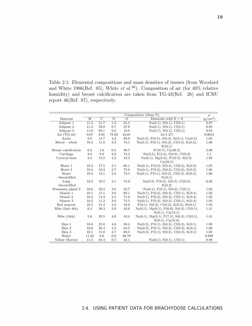
Table 2.1 lists the tissue compositions taken from Woodard and White85 and White
et al.86 (also listed in ICRU report 46 (Ref. 87)) that are used in the brachytherapy
phantoms in this thesis.
2.4.2 Tools for files in DICOM format
Clinical patient data files are most often stored in a format that follows the interna-
tional standard, DICOM (Digital Imaging and Communications in Medicine)88 which
2.4. USING PATIENT DATA FOR BRACHYDOSE CALCULATIONS
19
Table 2.1: Elemental compositions and mass densities of tissues (from Woodardand White 1986(Ref. 85), White et al.86). Composition of air (for 40% relativehumidity) and breast calcification are taken from TG-43(Ref. 26) and ICRUreport 46(Ref. 87), respectively.
Composition (Mass %) ρMaterial H C N O Elements with Z > 8 (g/cm3)
Adipose 1 11.2 51.7 1.3 35.5 Na(0.1), S(0.1), Cl(0.1) 0.97Adipose 2 11.4 59.8 0.7 27.8 Na(0.1), S(0.1), Cl(0.1) 0.95Adipose 3 11.6 68.1 0.2 19.8 Na(0.1), S(0.1), Cl(0.1) 0.93
Air (TG-43) 0.07 0.01 75.03 23.61 Ar(1.27) 0.0012Aorta 9.9 14.7 4.2 69.8 Na(0.2), P(0.4), S(0.3), K(0.1), Ca(0.4) 1.05
Blood – whole 10.2 11.0 3.3 74.5 Na(0.1), P(0.1), S(0.2), Cl(0.3), K(0.2), 1.06Fe(0.1)
Breast calcification 0.3 1.6 0.5 40.7 P(18.7), Ca(38.2) 3.06Cartilage 9.6 9.9 2.2 74.4 Na(0.5), P(2.2), S(0.9), Cl(0.3) 1.1
Cortical bone 3.4 15.5 4.2 43.5 Na(0.1), Mg(0.2), P(10.3), S(0.3), 1.92Ca(22.5)
Heart 1 10.3 17.5 3.1 68.1 Na(0.1), P(0.2), S(0.2), Cl(0.2), K(0.3) 1.05Heart 3 10.4 10.3 2.7 75.6 Na(0.1), P(0.2), S(0.2), Cl(0.2), K(0.3) 1.05Heart 10.3 12.1 3.2 73.4 Na(0.1), P(0.1), S(0.2), Cl(0.3), K(0.2), 1.06
–blood-filled Fe(0.1)Lung 10.3 10.5 3.1 74.9 Na(0.2), P(0.2), S(0.3), Cl(0.3), 0.26
–blood-filled K(0.2)Mammary gland 2 10.6 33.2 3.0 52.7 Na(0.1), P(0.1), S(0.2), Cl(0.1) 1.02
Muscle 1 10.1 17.1 3.6 68.1 Na(0.1), P(0.2), S(0.3), Cl(0.1), K(0.4) 1.05Muscle 2 10.2 14.3 3.4 71.0 Na(0.1), P(0.2), S(0.3), Cl(0.1), K(0.4) 1.05Muscle 3 10.2 11.2 3.0 74.5 Na(0.1), P(0.2), S(0.3), Cl(0.1), K(0.4) 1.05
Red marrow 10.5 41.4 3.4 43.9 P(0.1), S(0.2), Cl(0.2), K(0.2), Fe(0.1) 1.03Ribs (2nd, 6th) 6.4 26.3 3.9 43.6 Na(0.1), Mg(0.1), P(6.0), S(0.3), Cl(0.1), 1.41
K(0.1), Ca(13.1)Ribs (10th) 5.6 23.5 4.0 43.4 Na(0.1), Mg(0.1), P(7.2), S(0.3), Cl(0.1), 1.41
K(0.1), Ca(15.6)Skin 1 10.0 25.0 4.6 59.4 Na(0.2), P(0.1), S(0.3), Cl(0.3), K(0.1) 1.09Skin 2 10.0 20.4 4.2 64.5 Na(0.2), P(0.1), S(0.2), Cl(0.3), K(0.1) 1.09Skin 3 10.1 15.8 3.7 69.5 Na(0.2), P(0.1), S(0.2), Cl(0.3), K(0.1) 1.09Water 11.22 0.0 0.0 88.78 0.998
Yellow Marrow 11.5 64.4 0.7 23.1 Na(0.1), S(0.1), Cl(0.1) 0.98
2.4. USING PATIENT DATA FOR BRACHYDOSE CALCULATIONS
20
has seen widespread adoption in hospitals and vendor software. To facilitate the use
of clinical patient files for the calculations in this thesis, C++ tools were developed to
interact with four DICOM file types:
CT image files: A tool set named “ct tools” was developed that reads in DICOM CT
images and converts them to an in-house, text-based data structure. The in-house
data structure is used to allow the application of image treatment algorithms (see
chapter 4) and to change phantom sizes through cropping or resampling. With a user
supplied CT mass density calibration and tissue assignment scheme, the CT data is
converted to the EGSnrc .egsphant file type which defines phantom voxel boundaries
and 3D arrays of voxel tissue assignments and mass densities.
RT dose files: Part of the extension of version 3.0 of the DICOM standard that deals
with radiotherapy file types, patient RT dose files contain dose distributions calculated
by treatment planning systems. These files are used to read DICOM meta-data that
are required when converting BrachyDose output into DICOM format.
RT plan files: These files contain the seed positions, radionuclides, and air-kerma
strengths of brachytherapy treatments that are being simulated. This information is
used to help generate input files for BrachyDose.
RT structure files: Contours defining patient organs and treatment volumes are de-
fined in this file type. These contours are used to calculate dose volume histograms
and clinical dose metrics as well as guiding the assignment of tissues when converting
from CT to .egsphant (see chapter 5).
2.4. USING PATIENT DATA FOR BRACHYDOSE CALCULATIONS
21
2.5 Simulation parameters
The majority of the simulations in this thesis are performed with the same parame-
ters. Seeds are fully modelled77 and, in most cases, are superimposed on a voxelized
geometry specified by EGSnrc phantom (.egsphant) files. Seed models, unless oth-
erwise stated, were previously benchmarked via calculations of the TG-43 dosimetry
parameters66. For all calculations, the photon energy cutoff is set to 1 keV and
Rayleigh scattering, bound Compton scattering, photoelectric absorption, and fluo-
rescent emission of characteristic K and L-shell x rays are modelled. Photon cross
sections are taken from the XCOM30 database and mass-energy absorption coeffi-
cients are calculated using the EGSnrc user-code g. Note that electron transport is
not modelled and dose in voxels is approximated by collision kerma.
2.5. SIMULATION PARAMETERS
Chapter 3
Breast tissue segmentation
Breast tissue generally consists of fibroglandular and adipose tissues, possibly with
some calcifications. The proportion of each of these tissues in a typical breast has been
studied by Yaffe et al.89 who found that the mean percentage of fibroglandular tissue
was 19.3% by volume. The dose to fibroglandular tissue is the quantity of interest in
mammography radiation protection89–92 and may also be relevant for brachytherapy
treatments as the linear attenuation coefficients of gland and tumour are similar93,94.
With the advent of 103Pd treatments, the use of 50 kV electronic brachytherapy
sources for partial breast irradiation, and the use of model-based dose calculation
algorithms, there is increasing interest in the role of breast tissue composition in
brachytherapy40,41,95.
At the time of the research presented in this chapter, current model-based prac-
tices in Monte Carlo simulations for brachytherapy typically used homogeneous aver-
aged tissues to represent different ratios of glandular and adipose tissue40,41. Some-
times, CT data were used to assign mass density to each voxel41. Photon transport
and energy deposition occured in these averaged tissues. While more recent work
began to investigate breast tissue segmentation96 and the importance of tissue seg-
mentation for kilovoltage beams97, the differences between the dose to the separate
glandular and adipose tissues had been largely ignored in treatment planning studies.
22
23
In mammography radiation protection, it is common to estimate the average
dose to the glandular tissue89–92 by transporting photons through an averaged tissue
and then calculating the portion of energy deposited in the fibroglandular tissue using
ratios of mass energy absorption coefficients. In effect, photon transport is modelled
in the averaged tissue and energy deposition to gland is calculated.
Prior to the work presented in this chapter, the question of the accuracy of
using homogeneous averaged tissues in breast calculations and under which conditions
their use might be justified in lieu of fully segmented phantoms had not yet been
thoroughly investigated. This chapter presents an investigation of the effects of more
realistic segmentation of breast tissues in model-based Monte Carlo breast dosimetry.
Possible inaccuracies may occur during the transport of particles through the breast
creating differences in the photon energy fluence, and during the deposition of dose
because of choices of dose scoring media and incorrect photon energy fluence. In
this chapter, the current model-based practices of brachytherapy and mammography
radiation protection are investigated and compared to fully segmented calculations.
The modelling of calcifications in the breast is also investigated.
3.1 Methods
In all calculations, sixty-four fully modelled77 TheraSeed (Theragenics Corporation,
Buford Georgia USA) 200 103Pd brachytherapy seeds (mean emerging photon energy
from seed of 20.71 keV (Ref. 98)) are placed in a cube formation centred around the
centre of the phantom, (0, 0, 0) cm, with central x, y, and z coordinates of ±1.55 cm
or ±0.55 cm and axes parallel to the z-axis. The 0.05 cm offsets were chosen so that
the centres of the seeds would not lie on voxel boundaries for (1 mm)3 voxel sizes. A
64 cm3 planning treatment volume (PTV) region is defined as a cube ranging from
3.1. METHODS
24
(2, 2, 2) cm to (-2, -2, -2) cm. As these dimensions represent a larger PTV and lower
seed density than the median clinical dimensions99, calculations are also performed
with seed central x, y, and z coordinates of ±0.92 cm or ±0.46 cm with a PTV ranging
from (1.23, 1.23, 1.23) cm to (-1.23, -1.23, -1.23) cm to approximate a clinically small,
dense treatment.
Simulations of 109 histories achieve statistical uncertainties of less than 0.2%
on the dose in voxels in the PTV. These high precision calculations, which each
take roughly 4.5 hours of CPU time on a single 3.0 GHz Woodcrest core, are not
necessarily needed for the calculation of DVHs as simulations of 107 histories produce
nearly indistinguishable curves.
Densities and elemental compositions of breast tissues and breast calcifications
are taken from Woodard and White (Ref. 85) and ICRU Report 46 (Ref. 87) respec-
tively (table 2.1, page 19). The averaged breast tissues in this work are specified as
percent mixtures by mass. For most calculations, proportions of 25% fibroglandular
tissue and 75% adipose tissue by mass (23.7% and 76.3% by volume) are used to
approximate the recommendations of Yaffe et al.89. Over the photon energy range
of 10 to 30 keV, the mass energy absorption coefficient ratios of fibroglandular tis-
sue, adipose tissue, and a 25% gland 75% adipose mixture (by mass) to water are
at 0.80 ± 0.01 (gland/water), 0.60 ± 0.01 (adipose/water), and 0.65 ± 0.01 ((25/75
mixture)/water).
Physical dose distributions and dose volume histograms are both calculated. To
investigate doses to adipose and fibroglandular tissues separately, an in-house code
was developed to allow the calculation of dose volume histograms (DVHs) wherein
the volume considered consists only of those voxels within the PTV containing one
medium (e.g., DVHs for voxels containing gland only).
3.1. METHODS
25
3.1.1 Dose to gland and adipose versus dose to an averaged
tissue
For this portion of the study a simple geometry configuration defined as a 12×12×12 cm3
phantom with (1 mm)3 voxels is used to approximate a breast brachytherapy treat-
ment; dose distributions are unchanged within statistics with (2 mm)3 voxels. The
PTV is at the centre of the phantom. The whole phantom is filled with an av-
eraged tissue of given proportions of gland and adipose or each voxel is randomly
assigned a single tissue so as to create a phantom with the same proportion of tis-
sues by mass. For example, one phantom has voxels containing a single averaged
tissue (25% gland, 75% adipose by mass) while the other has each voxel randomly
assigned gland or adipose so as to maintain this proportion by mass over the entire
phantom. These phantoms are called “25/75-averaged-tissue phantom” and “25/75-
randomly-segmented phantom” respectively and the averaged tissue is denoted by
“25/75-averaged-tissue”. In general, the naming scheme used in this work is [propor-
tions of gland/adipose(/calcification) by mass]-[segmentation model]. For the aver-
aged tissue phantoms, dose is scored either in the averaged tissue (to investigate the
method often used in brachytherapy calculations) or in fibroglandular tissue (to in-
vestigate the method used for mammography radiation protection studies89–91 albeit
with a much different source geometry) (see page 16 for a description of scoring dose
to fictitious voxel media). For randomly segmented phantoms, dose is scored in the
tissue of each particular voxel.
These phantoms are used to investigate the hypothesis that the photon energy
fluence remains relatively unchanged between an averaged tissue phantom and a ran-
domly segmented phantom. Assuming this is the case, these phantoms can provide
information concerning dose differences that arise from modelling gland and adipose
3.1. METHODS
26
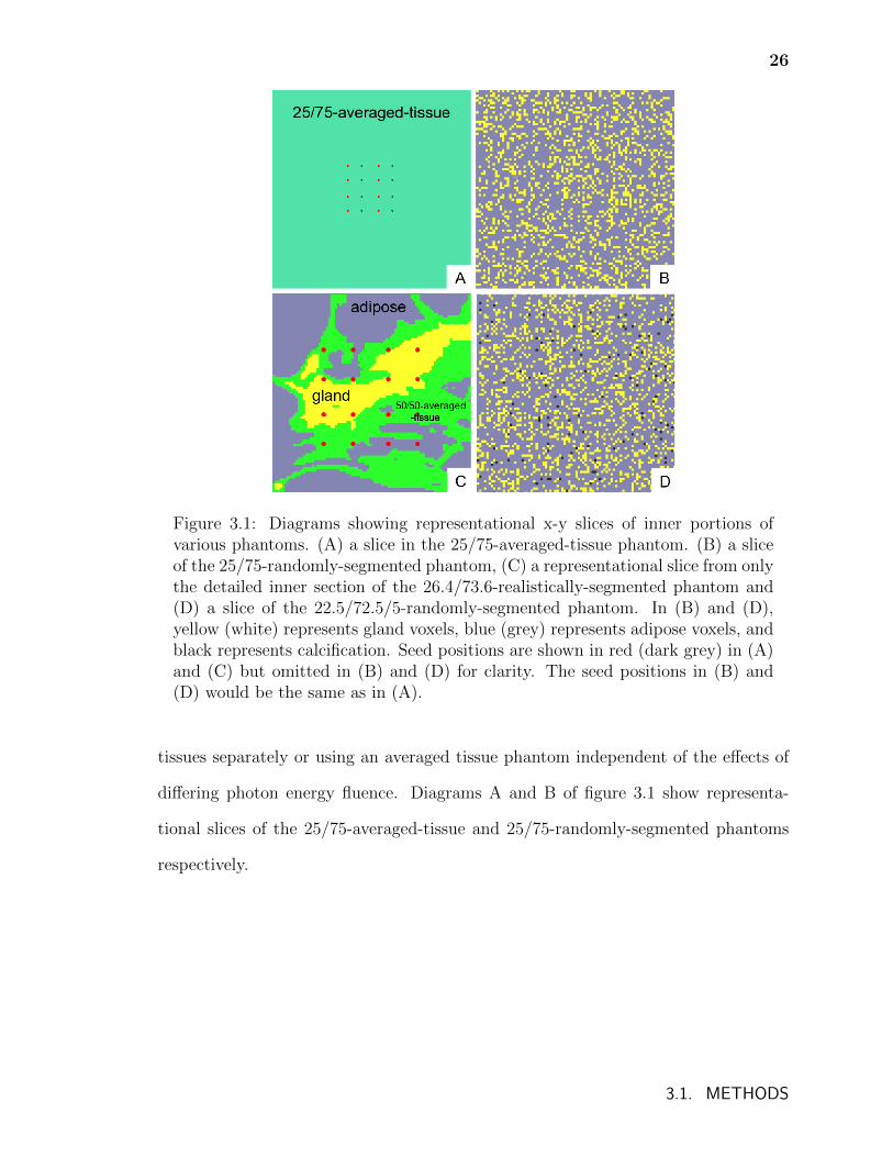
Figure 3.1: Diagrams showing representational x-y slices of inner portions ofvarious phantoms. (A) a slice in the 25/75-averaged-tissue phantom. (B) a sliceof the 25/75-randomly-segmented phantom, (C) a representational slice from onlythe detailed inner section of the 26.4/73.6-realistically-segmented phantom and(D) a slice of the 22.5/72.5/5-randomly-segmented phantom. In (B) and (D),yellow (white) represents gland voxels, blue (grey) represents adipose voxels, andblack represents calcification. Seed positions are shown in red (dark grey) in (A)and (C) but omitted in (B) and (D) for clarity. The seed positions in (B) and(D) would be the same as in (A).
tissues separately or using an averaged tissue phantom independent of the effects of
differing photon energy fluence. Diagrams A and B of figure 3.1 show representa-
tional slices of the 25/75-averaged-tissue and 25/75-randomly-segmented phantoms
respectively.
3.1. METHODS
27
3.1.2 Effect of realistic segmentation on photon energy
fluence
To approximate a realistically segmented breast, a phantom was created using a nu-
merical breast phantom from the work of Zastrow et al.100 Breast phantom 070604PA1
was chosen because its proportions are nearly 25% gland and 75% adipose by mass.
This phantom contains three classes of fibroglandular and adipose tissues that differ
in their dielectric properties. Voxels in the Zastrow phantom containing any class of
fibroglandular (adipose) tissue are set to the fibroglandular (adipose) tissue (compo-
sition found in table 2.1, page 19) in the phantoms for the present work. The numer-
ical phantom also contains a so-called transitional tissue (having dielectric properties
transitioning between gland and adipose) which is approximated in the phantoms for
the present work as being 50% adipose and 50% fibroglandular tissues by mass. The
centre of the phantom for the present work is set to (0, 0, 0) cm and a 5 × 5 × 5 cm3
centred cube of 0.5 × 0.5 × 0.5 mm3 voxels is taken from the numerical phantom of
voxels of the same size. The 5 × 5 × 5 cm3 detailed cube is surrounded by single,
large voxels of adipose tissue that extend to the outer dimensions of the numerical
phantom (x = ± 7.5 cm, y = ± 9.55 cm, z = ± 6.75 cm). In the detailed cube, 9%
of voxels are gland, 31% are 50/50 gland/adipose, and 60% are adipose (see a typical
slice in figure 3.1 C). A second phantom is also created that is identical except that the
detailed 5 × 5 × 5 cm3 cube is filled with voxels of an averaged tissue with the same
proportions by mass as the segmented detailed cube (26.4% fibroglandular and 73.6%
adipose tissue). These phantoms are called “26.4/73.6-realistically-segmented phan-
tom” and “26.4/73.6-averaged-tissue phantom” respectively and the averaged tissue
is denoted by “26.4/73.6-averaged-tissue”. The position of the seeds and PTV remain
the same as those of the randomly segmented phantom as they lie approximately in
3.1. METHODS
28
the centre of the distribution of fibroglandular tissue.
To approximate the use of CT data to assign voxel densities, an additional mod-
ified averaged tissue phantom is created such that each voxel contains the averaged
tissue material but with voxel densities identical to that of the realistically segmented
phantom.
A second realistically segmented phantom is also created using another com-
putational phantom from Zastrow et al. to confirm that the general trend of the
results found are not dependent on the particular glandular density of the 26.5/73.6-
realistically-segmented phantom. This denser phantom is composed of approximately
55% fibroglandular and 45% adipose tissues.
3.1.3 The effect of calcifications on photon energy fluence
A randomly segmented phantom is created composed of 22.5% fibroglandular tissue,
72.5% adipose tissue and 5% calcification by mass (22.1%, 76.3% and 1.6% by volume
respectively) with calcified (1 mm)3 voxels distributed randomly throughout the entire
phantom. The fraction of calcification was chosen based on results found in the litera-
ture101,102. While the dimensions of 1 × 1 × 1 mm3 used may be too small to represent
the size of an average calcification, it serves well as a limiting case scenario; if small,
randomly distributed calcifications significantly effect the ability to approximate the
photon energy fluence with an averaged tissue, then larger ones will have an effect.
This phantom is compared to an averaged tissue phantom of the same proportions, a
second averaged tissue phantom where the density of each voxel matches that of the
same voxel in the randomly segmented phantom, and a third averaged tissue phantom
composed of 25% gland, 75% adipose with the same voxel densities as the randomly
segmented phantom (that includes calcifications). The randomly segmented and av-
3.1. METHODS
29
eraged tissue phantoms are denoted by “22.5/72.5/5-randomly-segmented phantom”
and “22.5/72.5/5-averaged-tissue phantom” respectively and the averaged tissue is
denoted by “22.5/72.5/5-averaged-tissue”. Diagram D of figure 3.1 shows a represen-
tational slice of the 22.5/72.5/5-randomly-segmented phantom.
3.2 Results and Discussion
3.2.1 Dose to gland and adipose versus dose to an averaged
tissue
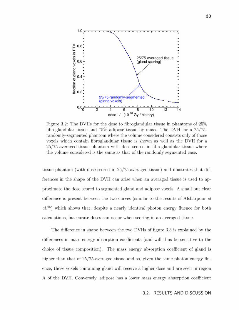
Figure 3.2 compares the DVHs for the dose to the gland voxels within the PTV of
the 25/75-randomly-segmented phantom to the dose to the voxels corresponding to
the same spatial coordinates of the 25/75-averaged-tissue phantom with dose scored
in gland. The close agreement between the two curves implies that the media in
the 25/75-randomly-segmented phantom are sufficiently uniformly distributed such
that, to first order, the photon energy fluence remains the same between the two
phantoms. This is confirmed by the fact that the explicitly calculated photon energy
fluences at the centre of each phantom agree within 2%. The agreement also implies
that, in the very unlikely case that a realistic breast is also sufficiently uniform in its
distribution of gland and adipose tissues (i.e., the photon energy fluence of a realistic
breast remains unchanged from that of an averaged tissue phantom), the method
used in mammography of photon transport in an averaged tissue and dose scoring in
a fibroglandular tissue would provide accurate dose volume metrics and mean doses
to glandular tissue.
Figure 3.3 compares the DVHs for the dose to the entire PTV for the 25/75-
randomly-segmented phantom (dose to gland and adipose voxels) and 25/75-averaged-
3.2. RESULTS AND DISCUSSION
30
0 2 4 6 8 10 12 14
dose / (10-13
Gy / history)
0.0
0.2
0.4
0.6
0.8
1.0
fractio
n o
f g
lan
d v
oxe
ls in
PT
V
25/75-averaged-tissue(gland scoring)
25/75-randomly-segmented (gland voxels)
Figure 3.2: The DVHs for the dose to fibroglandular tissue in phantoms of 25%fibroglandular tissue and 75% adipose tissue by mass. The DVH for a 25/75-randomly-segmented phantom where the volume considered consists only of thosevoxels which contain fibroglandular tissue is shown as well as the DVH for a25/75-averaged-tissue phantom with dose scored in fibroglandular tissue wherethe volume considered is the same as that of the randomly segmented case.
tissue phantom (with dose scored in 25/75-averaged-tissue) and illustrates that dif-
ferences in the shape of the DVH can arise when an averaged tissue is used to ap-
proximate the dose scored to segmented gland and adipose voxels. A small but clear
difference is present between the two curves (similar to the results of Afsharpour et
al.96) which shows that, despite a nearly identical photon energy fluence for both
calculations, inaccurate doses can occur when scoring in an averaged tissue.
The difference in shape between the two DVHs of figure 3.3 is explained by the
differences in mass energy absorption coefficients (and will thus be sensitive to the
choice of tissue composition). The mass energy absorption coefficient of gland is
higher than that of 25/75-averaged-tissue and so, given the same photon energy flu-
ence, those voxels containing gland will receive a higher dose and are seen in region
A of the DVH. Conversely, adipose has a lower mass energy absorption coefficient
3.2. RESULTS AND DISCUSSION
31
0 2 4 6 8 10 12 14
dose / (10-13
Gy / history)
0.0
0.2
0.4
0.6
0.8
1.0
fra
ctio
n o
f P
TV
25/75-avg.-tissue (25/75-avg.-tissue scoring)
25/75-randomly-seg.(all voxels)
A
B
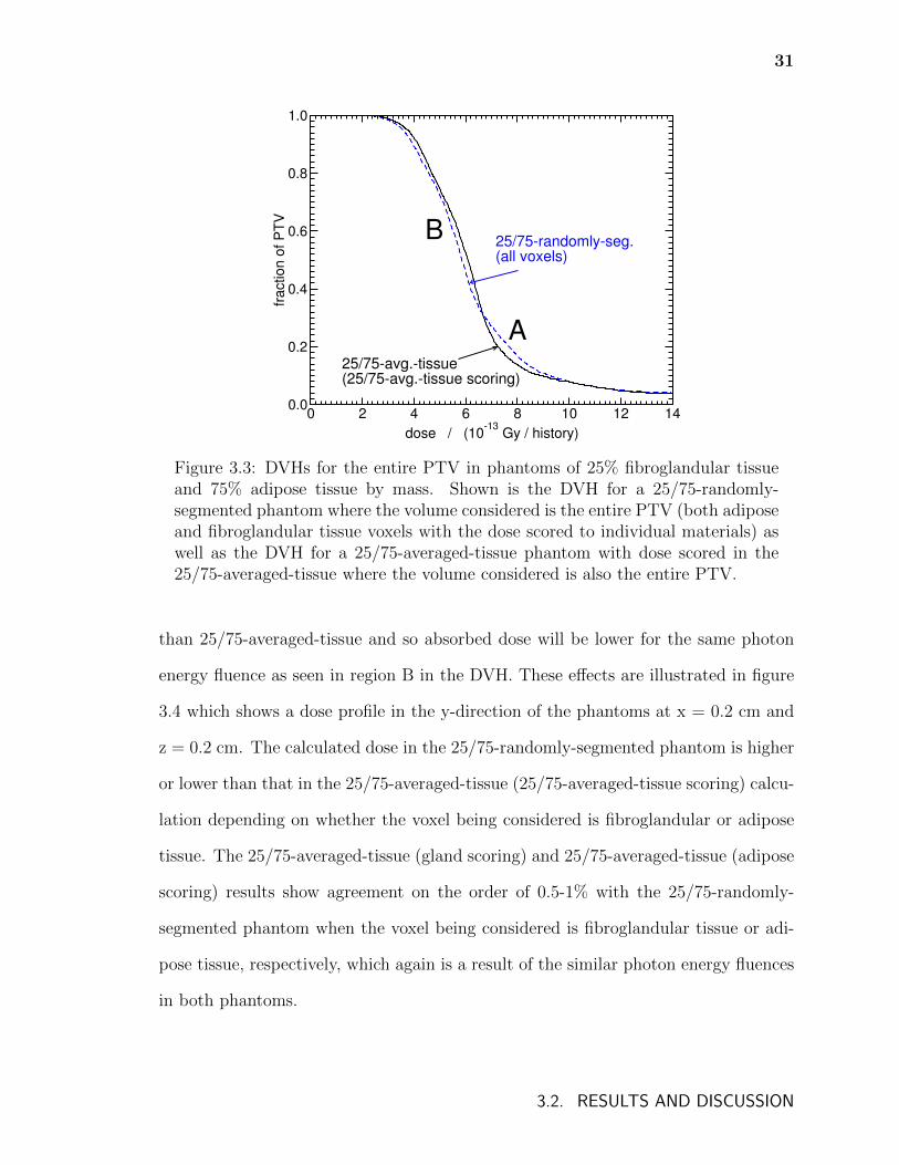
Figure 3.3: DVHs for the entire PTV in phantoms of 25% fibroglandular tissueand 75% adipose tissue by mass. Shown is the DVH for a 25/75-randomly-segmented phantom where the volume considered is the entire PTV (both adiposeand fibroglandular tissue voxels with the dose scored to individual materials) aswell as the DVH for a 25/75-averaged-tissue phantom with dose scored in the25/75-averaged-tissue where the volume considered is also the entire PTV.
than 25/75-averaged-tissue and so absorbed dose will be lower for the same photon
energy fluence as seen in region B in the DVH. These effects are illustrated in figure
3.4 which shows a dose profile in the y-direction of the phantoms at x = 0.2 cm and
z = 0.2 cm. The calculated dose in the 25/75-randomly-segmented phantom is higher
or lower than that in the 25/75-averaged-tissue (25/75-averaged-tissue scoring) calcu-
lation depending on whether the voxel being considered is fibroglandular or adipose
tissue. The 25/75-averaged-tissue (gland scoring) and 25/75-averaged-tissue (adipose
scoring) results show agreement on the order of 0.5-1% with the 25/75-randomly-
segmented phantom when the voxel being considered is fibroglandular tissue or adi-
pose tissue, respectively, which again is a result of the similar photon energy fluences
in both phantoms.
3.2. RESULTS AND DISCUSSION
32
-4 -2 0 2 4y-position / cm
0
2
4
6
8
10
do
se
/ 1
0-1
3 G
y /
his
tory
25/75-avg.-tissue(gland scoring)
25/75-randomly seg.
25/75-avg.-tissue(25/75-avg.-tissue scoring)
25/75-avg.-tissue(adipose scoring)
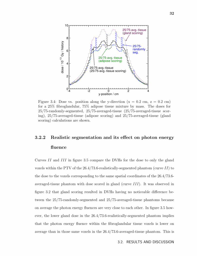
Figure 3.4: Dose vs. position along the y-direction (x = 0.2 cm, z = 0.2 cm)for a 25% fibroglandular, 75% adipose tissue mixture by mass. The doses for25/75-randomly-segmented, 25/75-averaged-tissue (25/75-averaged-tissue scor-ing), 25/75-averaged-tissue (adipose scoring) and 25/75-averaged-tissue (glandscoring) calculations are shown.
3.2.2 Realistic segmentation and its effect on photon energy
fluence
Curves II and III in figure 3.5 compare the DVHs for the dose to only the gland
voxels within the PTV of the 26.4/73.6-realistically-segmented phantom (curve II) to
the dose to the voxels corresponding to the same spatial coordinates of the 26.4/73.6-
averaged-tissue phantom with dose scored in gland (curve III). It was observed in
figure 3.2 that gland scoring resulted in DVHs having no noticeable difference be-
tween the 25/75-randomly-segmented and 25/75-averaged-tissue phantoms because
on average the photon energy fluences are very close to each other. In figure 3.5 how-
ever, the lower gland dose in the 26.4/73.6-realistically-segmented phantom implies
that the photon energy fluence within the fibroglandular tissue voxels is lower on
average than in those same voxels in the 26.4/73.6-averaged-tissue phantom. This is
3.2. RESULTS AND DISCUSSION
33
0 2 4 6 8 10 12 14
dose / (10-13
Gy / history)
0.0
0.2
0.4
0.6
0.8
1.0
fra
ctio
n o
f re
leva
nt
vo
xe
ls in
PT
V
26.4/73.6-real.-seg. (gland voxels)
26.4/73.6-avg.-tissue (gland scoring)
26.4/73.6-realistic-seg.(all voxels)
III
I
II
26.4/73.6-real.-seg.(adipose voxels)
26.4/73.6-avg.-tissue(adipose scoring)
V
IV
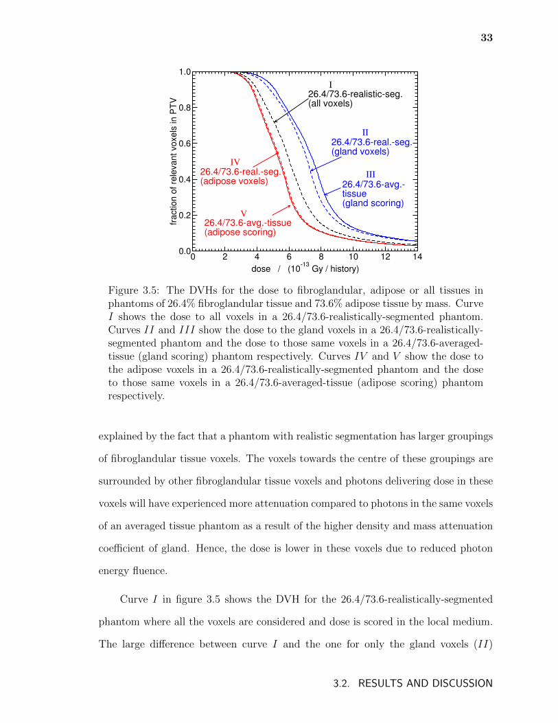
Figure 3.5: The DVHs for the dose to fibroglandular, adipose or all tissues inphantoms of 26.4% fibroglandular tissue and 73.6% adipose tissue by mass. CurveI shows the dose to all voxels in a 26.4/73.6-realistically-segmented phantom.Curves II and III show the dose to the gland voxels in a 26.4/73.6-realistically-segmented phantom and the dose to those same voxels in a 26.4/73.6-averaged-tissue (gland scoring) phantom respectively. Curves IV and V show the dose tothe adipose voxels in a 26.4/73.6-realistically-segmented phantom and the doseto those same voxels in a 26.4/73.6-averaged-tissue (adipose scoring) phantomrespectively.
explained by the fact that a phantom with realistic segmentation has larger groupings
of fibroglandular tissue voxels. The voxels towards the centre of these groupings are
surrounded by other fibroglandular tissue voxels and photons delivering dose in these
voxels will have experienced more attenuation compared to photons in the same voxels
of an averaged tissue phantom as a result of the higher density and mass attenuation
coefficient of gland. Hence, the dose is lower in these voxels due to reduced photon
energy fluence.
Curve I in figure 3.5 shows the DVH for the 26.4/73.6-realistically-segmented
phantom where all the voxels are considered and dose is scored in the local medium.
The large difference between curve I and the one for only the gland voxels (II)
3.2. RESULTS AND DISCUSSION
34
illustrates the need to treat each tissue individually if the dose to a single tissue is of
interest.
Curves IV and V in figure 3.5 compare the DVHs for the dose to only the adipose
voxels within the PTV of the 26.4/73.6-realistically-segmented phantom (IV ) to the
dose to the same voxels of the 26.4/73.6-averaged-tissue phantom with dose scored
in adipose (V ). The larger groupings of adipose tissue (compared to a randomly
segmented phantom) will cause the photon energy fluence in those voxels to be higher
in a realistically segmented phantom than in the same voxels in an averaged tissue
phantom. However, as the averaged tissue is 73.6% adipose by mass, the differences
in photon energy fluence in the adipose tissue groupings will be less dramatic than in
the case of gland tissue. This is reflected in the close agreement between curves IV
and V .
Figure 3.6 compares the DVHs for the dose to the entire PTV for the 26.4/73.6-
realistically-segmented phantom with the dose scored in each medium and the 26.4/73.6-
averaged-tissue phantom with dose scored in 26.4/73.6-averaged-tissue. While the
differences between the DVHs are qualitatively similar to those of figure 3.3, they
are smaller in magnitude. In this case, the change in photon energy fluence implied
by figure 3.5 compensates to some degree for the change in scored dose as a result
of scoring in gland and adipose versus averaged tissue (regions A and B in figure
3.3). These competing effects combine to produce a calculation that provides more
accurate dose volume histograms when considering the DVH for all PTV voxels.
Additionally, the differences seen in the comparison of curves II and III in
figure 3.5 reflect the inaccuracy of using the photon energy fluence in an averaged
tissue to approximate the photon energy fluence in the gland voxels of a realistically
segmented phantom. The gland voxels in a realistically segmented phantom will
have a lower photon energy fluence on average than the same voxels of an averaged
3.2. RESULTS AND DISCUSSION
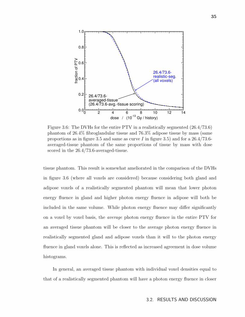
35
0 2 4 6 8 10 12 14
dose / (10-13
Gy / history)
0.0
0.2
0.4
0.6
0.8
1.0
fra
ctio
n o
f P
TV
26.4/73.6-realistic-seg. (all voxels)
26.4/73.6-averaged-tissue (26.4/73.6-avg.-tissue scoring)
Figure 3.6: The DVHs for the entire PTV in a realistically segmented (26.4/73.6)phantom of 26.4% fibroglandular tissue and 76.3% adipose tissue by mass (sameproportions as in figure 3.5 and same as curve I in figure 3.5) and for a 26.4/73.6-averaged-tissue phantom of the same proportions of tissue by mass with dosescored in the 26.4/73.6-averaged-tissue.
tissue phantom. This result is somewhat ameliorated in the comparison of the DVHs
in figure 3.6 (where all voxels are considered) because considering both gland and
adipose voxels of a realistically segmented phantom will mean that lower photon
energy fluence in gland and higher photon energy fluence in adipose will both be
included in the same volume. While photon energy fluence may differ significantly
on a voxel by voxel basis, the average photon energy fluence in the entire PTV for
an averaged tissue phantom will be closer to the average photon energy fluence in
realistically segmented gland and adipose voxels than it will to the photon energy
fluence in gland voxels alone. This is reflected as increased agreement in dose volume
histograms.
In general, an averaged tissue phantom with individual voxel densities equal to
that of a realistically segmented phantom will have a photon energy fluence in closer
3.2. RESULTS AND DISCUSSION
36
agreement with that of the realistically segmented phantom. However, as the densi-
ties of gland and adipose differ to a much smaller degree than the mass attenuation
coefficients (approximately 7% vs. 20% difference respectively), the modeling of vox-
els of varying density does not fully overcome the differences in photon energy fluence.
For example, in figure 3.5, the difference between the minimum dose that 90% of the
volume receives (D90) for the 26.4/73.6-realistically-segmented (gland voxels) calcu-
lation and the 26.4/73.6-averaged-tissue (gland scoring) calculation is approximately
6.3%. The use of a 26.4/73.6-averaged-tissue phantom with voxel densities equal to
that of the 26.4/73.6-realistically-segmented phantom (not shown) only reduces the
difference to 4.9%.
It is important to note that the improvement in dose volume metrics that would
result from improved simulation of photon energy fluence would only occur if one
was considering the dose to either gland or adipose. The inaccuracy of using an
averaged tissue phantom when the dose to gland is desired results from inaccurate
photon energy fluence alone and so, any improvement in photon energy fluence will
lead to improvement in dose volume metrics. In contrast, for dose to an entire volume
(both gland and adipose), what accuracy exists in DVHs (figure 3.6) is a result of
the competing effects of inaccurate photon energy fluence and inaccuracies from dose
scored in averaged tissue rather than gland and adipose (regions A and B in figure
3.3). Consequently, an improvement in photon energy fluence simulation will nullify
the competing effect and the differences shown in figure 3.3 will resurface.
A second realistically segmented phantom was created using another computa-
tional phantom from Zastrow et al.100. This phantom was composed of approximately
55% fibroglandular and 45% adipose tissues. The effects found in figures 3.5 and 3.6
were qualitatively identical but with slightly differing magnitude with this denser
phantom, confirming that the results of this work are not unique to the particular
3.2. RESULTS AND DISCUSSION
37
glandular density in the phantom used.
The results from the simulations with a seed configuration approximating a small,
dense treatment (not presented) confirm the general effects and their relative magni-
tudes discussed above.
In all calculations, the choice of tissue compositions can significantly affect the
dose calculated in the breast. For instance, the compositions in Hammerstein et al.90
could be used instead of those of Woodard and White and this choice would affect
the magnitude of the effects discussed in this work (e.g., the mass energy absorption
coefficient for gland at 20 keV is 17% lower for the composition in Woodard and
White than that in Hammerstein et al.90) but would not change the conclusions.
3.2.3 The effect of calcifications
A 22.5/72.5/5-randomly-segmented phantom with 22.5% fibroglandular tissue, 72.5%
adipose tissue and 5% calcification by mass was created. In figure 3.7, the DVH for
the dose to the fibroglandular voxels within the PTV is compared to the DVH of the
voxels corresponding to the same spatial coordinates for a 22.5/72.5/5-averaged-tissue
phantom (gland scoring). The lower dose for the 22.5/72.5/5-randomly-segmented
phantom shows that, despite the media being randomly distributed, calcifications in
the breast significantly lower the average photon energy fluence.
Figure 3.8 contains DVHs calculated for the entire PTV. Curve I shows the
DVH for the entire PTV for the 22.5/72.5/5-randomly-segmented phantom. The dis-
agreement between curve I and the DVH for the 22.5/72.5/5-averaged-tissue phantom
with dose scored in 22.5/72.5/5-averaged-tissue (curve II) shows that the difference in
photon energy fluence between the 22.5/72.5/5-randomly-segmented phantom and the
22.5/72.5/5-averaged-tissue phantom is too large to be compensated for by changes in
3.2. RESULTS AND DISCUSSION
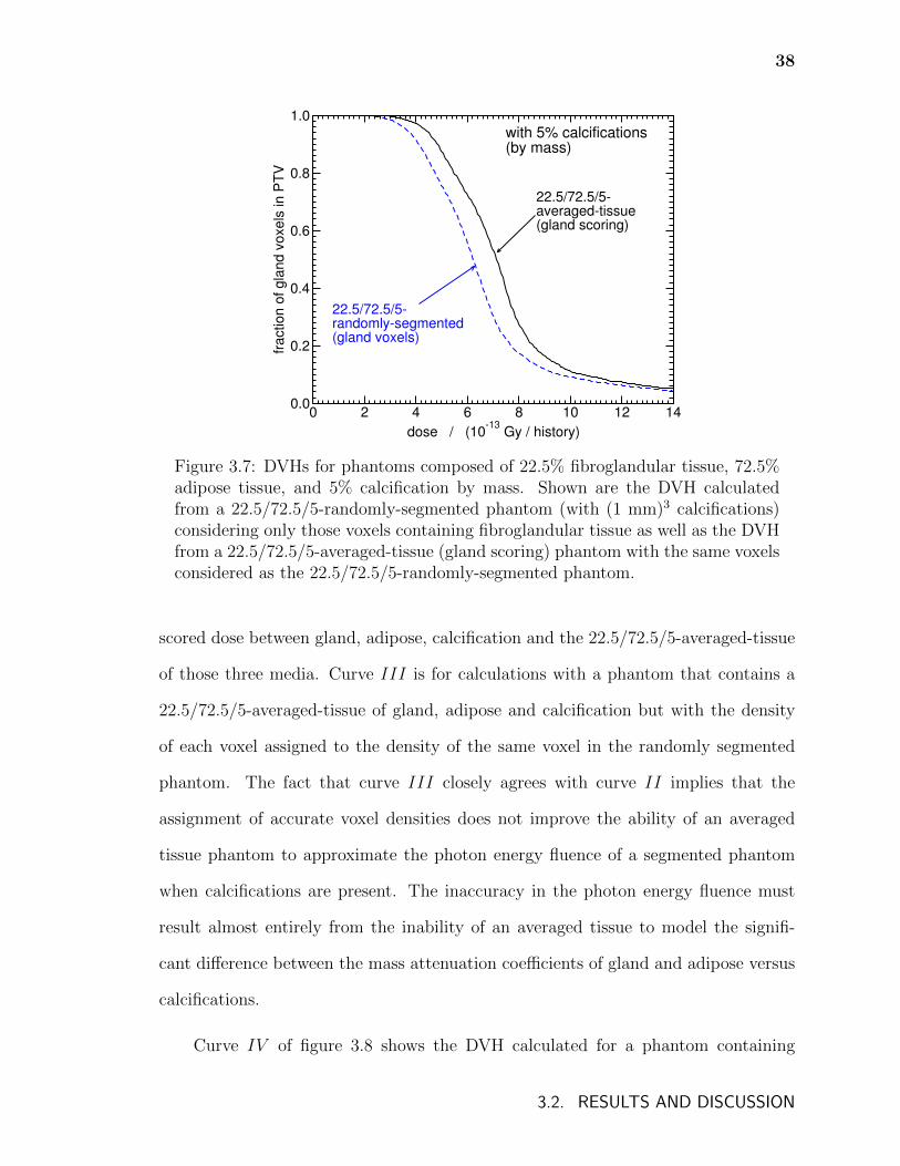
38
0 2 4 6 8 10 12 14
dose / (10-13
Gy / history)
0.0
0.2
0.4
0.6
0.8
1.0
fractio
n o
f g
lan
d v
oxe
ls in
PT
V
22.5/72.5/5-averaged-tissue(gland scoring)
22.5/72.5/5-randomly-segmented(gland voxels)
with 5% calcifications(by mass)
Figure 3.7: DVHs for phantoms composed of 22.5% fibroglandular tissue, 72.5%adipose tissue, and 5% calcification by mass. Shown are the DVH calculatedfrom a 22.5/72.5/5-randomly-segmented phantom (with (1 mm)3 calcifications)considering only those voxels containing fibroglandular tissue as well as the DVHfrom a 22.5/72.5/5-averaged-tissue (gland scoring) phantom with the same voxelsconsidered as the 22.5/72.5/5-randomly-segmented phantom.
scored dose between gland, adipose, calcification and the 22.5/72.5/5-averaged-tissue
of those three media. Curve III is for calculations with a phantom that contains a
22.5/72.5/5-averaged-tissue of gland, adipose and calcification but with the density
of each voxel assigned to the density of the same voxel in the randomly segmented
phantom. The fact that curve III closely agrees with curve II implies that the
assignment of accurate voxel densities does not improve the ability of an averaged
tissue phantom to approximate the photon energy fluence of a segmented phantom
when calcifications are present. The inaccuracy in the photon energy fluence must
result almost entirely from the inability of an averaged tissue to model the signifi-
cant difference between the mass attenuation coefficients of gland and adipose versus
calcifications.
Curve IV of figure 3.8 shows the DVH calculated for a phantom containing
3.2. RESULTS AND DISCUSSION
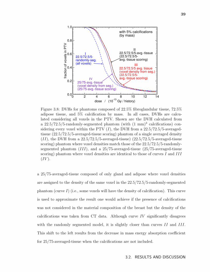
39
0 2 4 6 8 10 12 14
dose / (10-13
Gy / history)
0.0
0.2
0.4
0.6
0.8
1.0
fra
ctio
n o
f vo
xe
ls in
PT
V
22.5/72.5/5-avg.-tissue(22.5/72.5/5-avg.-tissue scoring)
22.5/72.5/5-randomly-seg.(all voxels)
with 5% calcifications(by mass)
25/75-avg.-tissue(voxel density from seg.)(25/75-avg.-tissue scoring)
22.5/72.5/5 avg. tissue(voxel density from seg.)(22.5/72.5/5-avg.-tissue scoring)IV
I
II
III
Figure 3.8: DVHs for phantoms composed of 22.5% fibroglandular tissue, 72.5%adipose tissue, and 5% calcification by mass. In all cases, DVHs are calcu-lated considering all voxels in the PTV. Shown are the DVH calculated froma 22.5/72.5/5-randomly-segmented phantom (with (1 mm)3 calcifications) con-sidering every voxel within the PTV (I), the DVH from a 22.5/72.5/5-averaged-tissue (22.5/72.5/5-averaged-tissue scoring) phantom of a single averaged density(II), the DVH from a 22.5/72.5/5-averaged-tissue) (22.5/72.5/5-averaged-tissuescoring) phantom where voxel densities match those of the 22.5/72.5/5-randomly-segmented phantom (III), and a 25/75-averaged-tissue (25/75-averaged-tissuescoring) phantom where voxel densities are identical to those of curves I and III(IV ).
a 25/75-averaged-tissue composed of only gland and adipose where voxel densities
are assigned to the density of the same voxel in the 22.5/72.5/5-randomly-segmented
phantom (curve I) (i.e., some voxels will have the density of calcification). This curve
is used to approximate the result one would achieve if the presence of calcifications
was not considered in the material composition of the breast but the density of the
calcifications was taken from CT data. Although curve IV significantly disagrees
with the randomly segmented model, it is slightly closer than curves II and III.
This shift to the left results from the decrease in mass energy absorption coefficient
for 25/75-averaged-tissue when the calcifications are not included.
3.2. RESULTS AND DISCUSSION
40
Figure 3.9 illustrates the effect of considering the dose to only the gland and
adipose in a phantom that contains calcifications. Curves I and II are identical to
curves I and II of figure 3.8. Curve III shows the DVH for only the gland and adipose
voxels of the 22.5/72.5/5-randomly-segmented phantom. As the voxels containing
calcification only correspond to 1.6% of total volume, the omission of the dose to the
calcifications has little effect on the DVH. This differs from curve IV which shows
the DVH for the voxels corresonding the same spatial coordinates of a 22.5/72.5/5-
averaged-tissue (25/75-averaged-tissue scoring) phantom. In this calculation, photon
transport occurs in an averaged tissue containing calcification but dose delivery in
an averaged tissue without calcification. While the elimination of calcification (and
its high Z contribution to composition) from the scoring averaged tissue moves curve
IV closer to agreement with curve III (compared to II versus I), the inability of
the 22.5/72.5/5-averaged-tissue phantom to approximate the photon energy fluence
of the 22.5/72.5/5-randomly-segmented phantom is clear.
3.3 Conclusions
The photon energy fluence is not accurately determined if an averaged tissue phantom
is used in Monte Carlo simulations. Given the typical composition of the breast89, if
the dose to gland tissue within the volume considered is desired, then the phantom
must be properly segmented to achieve accurate doses and dose volume metrics. If
dose to adipose tissue is desired, then an averaged tissue (adipose scoring) phantom
may be sufficient to achieve accurate dose volume metrics. If dose metrics for the
entire volume (all tissues) are desired and dose is scored in an averaged tissue, in-
accuracies in the photon energy fluence will partially compensate for inaccuracies in
scoring dose in an averaged tissue rather than in gland and adipose separately. While
3.3. CONCLUSIONS
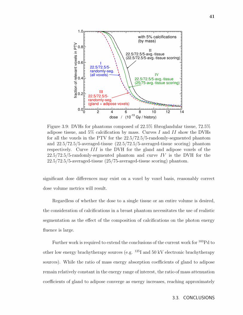
41
0 2 4 6 8 10 12 14
dose / (10-13
Gy / history)
0.0
0.2
0.4
0.6
0.8
1.0
fra
ctio
n o
f re
leva
nt
vo
xe
ls in
PT
V
22.5/72.5/5-avg.-tissue(22.5/72.5/5-avg.-tissue scoring)
22.5/72.5/5-randomly-seg.(all voxels)
with 5% calcifications(by mass)
22.5/72.5/5-randomly-seg.(gland + adipose voxels)
III
I
II
22.5/72.5/5-avg.-tissue(25/75-avg.-tissue scoring)
IV
Figure 3.9: DVHs for phantoms composed of 22.5% fibroglandular tissue, 72.5%adipose tissue, and 5% calcification by mass. Curves I and II show the DVHsfor all the voxels in the PTV for the 22.5/72.5/5-randomly-segmented phantomand 22.5/72.5/5-averaged-tissue (22.5/72.5/5-averaged-tissue scoring) phantomrespectively. Curve III is the DVH for the gland and adipose voxels of the22.5/72.5/5-randomly-segmented phantom and curve IV is the DVH for the22.5/72.5/5-averaged-tissue (25/75-averaged-tissue scoring) phantom.
significant dose differences may exist on a voxel by voxel basis, reasonably correct
dose volume metrics will result.
Regardless of whether the dose to a single tissue or an entire volume is desired,
the consideration of calcifications in a breast phantom necessitates the use of realistic
segmentation as the effect of the composition of calcifications on the photon energy
fluence is large.
Further work is required to extend the conclusions of the current work for 103Pd to
other low energy brachytherapy sources (e.g. 125I and 50 kV electronic brachytherapy
sources). While the ratio of mass energy absorption coefficients of gland to adipose
remain relatively constant in the energy range of interest, the ratio of mass attenuation
coefficients of gland to adipose converge as energy increases, reaching approximately
3.3. CONCLUSIONS
42
1.05 at 50 keV. It is expected that the observed effects are not as important for
higher-energy sources such as 192Ir because the mass energy absorption and mass
attenuation coefficients of the breast tissues are in much closer agreement at these
photon energies.
The assignment of voxel densities based on CT data to an averaged tissue phan-
tom reduces differences seen in photon energy fluence but not to such a degree that
differences in dose volume metrics disappear.
It is likely that the methods commonly used in mammography radiation protec-
tion calculations overestimate the average dose to the glandular tissue. This arises
because averaged tissue phantoms do not accurately reflect the photon energy fluence
in the gland of a realistic breast.
3.3. CONCLUSIONS
Chapter 4
Exploring model-based dose calculations for
125I lung brachytherapy
Although 125I lung brachytherapy has enjoyed considerable success, the standard prac-
tices for dosimetry and treatment planning involve significant approximations. Due to
the clinical nature of the implant, the final placement of the seeds cannot be precisely
predetermined and a simple nomogram of planar implant is used for pre-planning9.
A seed activity look up table is used to determine the intended row spacing of the
seeds to achieve approximately 100 Gy at a central point 5 mm from the plane of
the implant. Post-treatment analysis typically involves computed tomography (CT)
imaging and contouring the suture line and other volumes of interest. In addition,
the seed positions are identified and dose calculation is performed according to the
TG-43 formalism25–27, i.e., seeds in a homogeneous water environment and no in-
terseed attenuation. Thus, clinical dose calculations for lung brachytherapy neglect
the highly heterogeneous lung geometry. In reality, the patient treatment geometry
involves lung and other tissues which differ in atomic composition and density from
water. Considering the significant differences in mass energy absorption and mass at-
tenuation coefficients of various tissues and water at the energies of photons emitted
by 125I seeds, it is expected that heterogeneities may significantly affect dosimetry for
lung brachytherapy24. While this was confirmed by a preliminary investigation55, no
43
44
calculations using voxelized patient data for permanent implant lung brachytherapy
had been reported before the work presented in this chapter.
The focus of this chapter is the application of full Monte Carlo simulations of
125I lung brachytherapy, including considerations that must be addressed in order for
patient CT data to be used in model-based dose calculation algorithms (MBDCA) for
lung brachytherapy. While many of the considerations are applicable to low-energy
brachytherapy in general and have been identified in the literature, changes in dose
as a result of these considerations have been infrequently reported and, in the case of
lung brachytherapy, have never been investigated.
In 125I lung brachytherapy, CT scans are taken after implantation of 125I seeds.
The high-Z, high density nature of these seeds leads to streaking artifacts which, if
uncorrected, may lead to large discrepancies between assigned and true voxel compo-
sitions and densities50. The correction of these CT artifacts presents a challenge due
to the small size and significant number of seeds. Approaches to mitigating artifacts
due to brachytherapy seeds remains an active area of research50–52. Additionally, a
naive use of CT data of small spatial dimensions may lead to a phantom model of
insufficient extent to accurately model back-scattered photons and so padding of the
CT data may be required.
Beyond ensuring the accuracy of the CT phantom, accurate assignment of mate-
rial composition and density to each voxel can pose a challenge. A sophisticated tissue
segmentation method – the stoichiometric method – has been introduced44; however,
this method may not be feasible in all clinics and its accuracy for low-energy photon
dose calculations is unknown. The degree of detail in the tissue assignment scheme
(i.e., number and choice of tissues) may have a significant effect on the dose. Finally,
the effect of errors in voxel density assignment on dose has not been studied.
45
In this chapter, Monte Carlo calculations are performed with the EGSnrc user-
code BrachyDose to determine dose distributions for six patients treated with intra-
operative 125I lung brachytherapy at the Mayo Clinic Rochester. Modelling consider-
ations as well as their effect on patient dose distributions are studied. Additionally,
doses calculated with the Monte Carlo technique are compared to those found via the
TG-43 approach.
4.1 Methods
Six patients were treated for stage I non-small cell lung cancer with 125I (GE Health-
care/Oncura, Arlington Heights IL USA, model 6711) mesh brachytherapy in conjunc-
tion with sublobar resection at the Mayo Clinic Rochester. Source air kerma strengths
ranged from approximately 0.70 µGy·m2/h to 0.86 µGy·m2/h. As per protocol Z4032
of the American College of Surgeons Oncology Group (2005), post-implant CT scans
(GE LightSpeed RT 16) were taken within 30 days of implantation. In each of the
anterior-posterior and lateral directions, the scans have 512 voxels with equal widths
ranging from approximately 0.02 cm to 0.04 cm for total image widths of approxi-
mately 11 cm to 20 cm. In the superior-inferior direction, the scans have a consistent
voxel width of 0.0625 cm with the number of voxels ranging from 125 to 253 for a
total image width ranging from 8 cm to 16 cm. From the CT images, seed positions
are determined, suture lines are contoured, and PTV structures are delineated from
the suture lines: PTV05, PTV07, PTV10, and PTV20 are 5 mm, 7 mm, 10 mm and
20 mm expansions of the suture line, respectively.
Seeds are fully modelled77 and are superimposed on a voxelized geometry spec-
ified by EGSnrc phantom files (.egsphant). Unless otherwise stated, dose is scored
in the local medium in each voxel. Simulations are performed with 2.7 × 10¹⁰ histo-
ries to achieve average statistical uncertainties of at most 0.2% in PTV20 volumes.
4.1. METHODS
46
Simulations of fewer histories achieving less than 2% average statistical uncertainty
in PTV05 volumes take less than 65 minutes on one 3.0 GHz Woodcrest core for
the small voxel sizes used (approximately 0.7 mm × 0.7 mm × 0.625 mm); running
calculations in parallel on a modest cluster of 30 cores would reduce calculations to
a couple of minutes.
4.1.1 Correcting metallic artifacts
Patient CT data contain streaking artifacts which result from the presence of forty
brachytherapy seeds in the treatment region. A number of methods are used to correct
CT data for these metallic artifacts.
The first metallic artifact reduction method considered, referred to in the fol-
lowing as virtual sinogram metallic artifact correction and denoted “vsMAR”, uses
a filtered back-projection on a modified virtual sinogram and is an example of a
projection completion method. This method, which employs a virtual sinogram,
was introduced by Abdoli et al.103,104 for circumstances when raw sinogram data are
unavailable and is a variation of similar methods using raw sinogram data49,105–107
often denoted “MAR”. In the MAR method, metallic objects in a CT image are
segmented using a CT number threshold. A metal-only image is extracted and the
image is forward projected to obtain a sinogram corresponding to metallic objects.
The metal-only sinogram is used to delineate the bins of raw sinogram data that
correspond to projections containing metallic artifacts. These bins are removed from
the sinogram and replaced by an interpolation of the surrounding projections. The
corrected sinogram is then reconstructed to produce an artifact-reduced image.
Raw sinogram data were unavailable for the patient CT data used in the present
work and hence the vsMAR method is used103,104. A virtual sinogram created by
4.1. METHODS
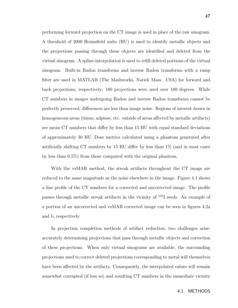
47
performing forward projection on the CT image is used in place of the raw sinogram.
A threshold of 2000 Hounsfield units (HU) is used to identify metallic objects and
the projections passing through these objects are identified and deleted from the
virtual sinogram. A spline-interpolation is used to refill deleted portions of the virtual
sinogram. Built-in Radon transforms and inverse Radon transforms with a ramp
filter are used in MATLAB (The Mathworks, Natick Mass. USA) for forward and
back projections, respectively; 180 projections were used over 180 degrees. While
CT numbers in images undergoing Radon and inverse Radon transforms cannot be
perfectly preserved, differences are less than image noise. Regions of interest drawn in
homogeneous areas (tissue, adpiose, etc. outside of areas affected by metallic artifacts)
see mean CT numbers that differ by less than 15 HU with equal standard deviations
of approximately 30 HU. Dose metrics calculated using a phantom generated after
artificially shifting CT numbers by 15 HU differ by less than 1% (and in most cases
by less than 0.5%) from those computed with the original phantom.
With the vsMAR method, the streak artifacts throughout the CT image are
reduced to the same magnitude as the noise elsewhere in the image. Figure 4.1 shows
a line profile of the CT numbers for a corrected and uncorrected image. The profile
passes through metallic streak artifacts in the vicinity of 125I seeds. An example of
a portion of an uncorrected and vsMAR corrected image can be seen in figures 4.2a
and b, respectively.
In projection completion methods of artifact reduction, two challenges arise:
accurately determining projections that pass through metallic objects and correction
of these projections. When only virtual sinograms are available, the surrounding
projections used to correct deleted projections corresponding to metal will themselves
have been affected by the artifacts. Consequently, the interpolated values will remain
somewhat corrupted (if less so) and resulting CT numbers in the immediate vicinity
4.1. METHODS
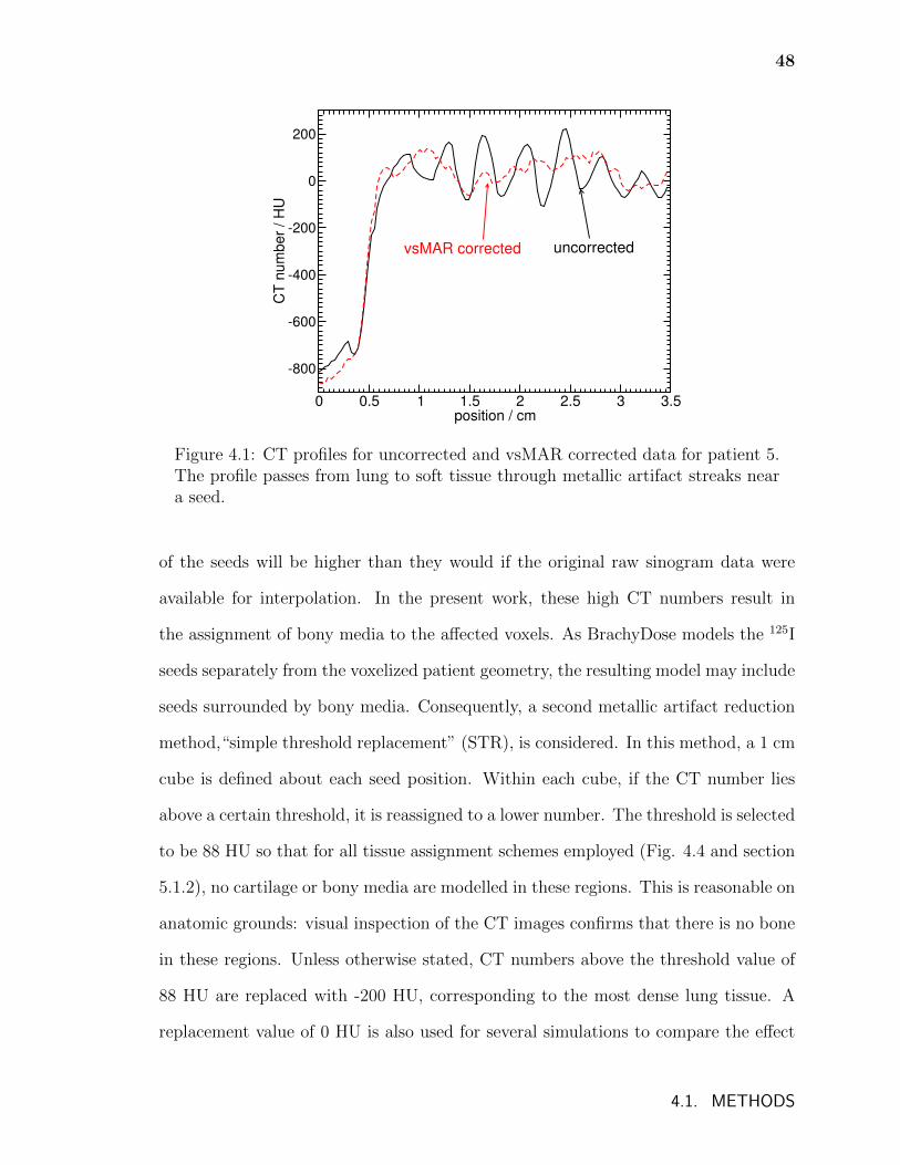
48
0 0.5 1 1.5 2 2.5 3 3.5position / cm
-800
-600
-400
-200
0
200
CT
num
ber
/ H
U
uncorrectedvsMAR corrected
Figure 4.1: CT profiles for uncorrected and vsMAR corrected data for patient 5.The profile passes from lung to soft tissue through metallic artifact streaks neara seed.
of the seeds will be higher than they would if the original raw sinogram data were
available for interpolation. In the present work, these high CT numbers result in
the assignment of bony media to the affected voxels. As BrachyDose models the 125I
seeds separately from the voxelized patient geometry, the resulting model may include
seeds surrounded by bony media. Consequently, a second metallic artifact reduction
method,“simple threshold replacement” (STR), is considered. In this method, a 1 cm
cube is defined about each seed position. Within each cube, if the CT number lies
above a certain threshold, it is reassigned to a lower number. The threshold is selected
to be 88 HU so that for all tissue assignment schemes employed (Fig. 4.4 and section
5.1.2), no cartilage or bony media are modelled in these regions. This is reasonable on
anatomic grounds: visual inspection of the CT images confirms that there is no bone
in these regions. Unless otherwise stated, CT numbers above the threshold value of
88 HU are replaced with -200 HU, corresponding to the most dense lung tissue. A
replacement value of 0 HU is also used for several simulations to compare the effect
4.1. METHODS
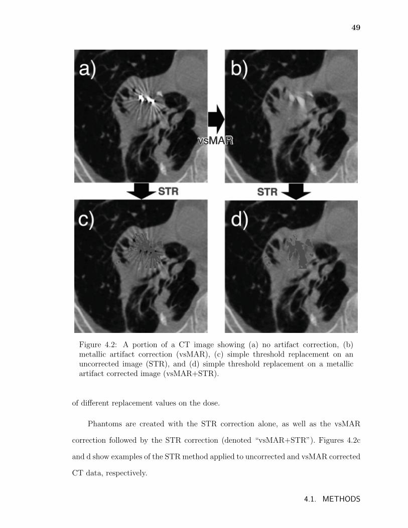
49
Figure 4.2: A portion of a CT image showing (a) no artifact correction, (b)metallic artifact correction (vsMAR), (c) simple threshold replacement on anuncorrected image (STR), and (d) simple threshold replacement on a metallicartifact corrected image (vsMAR+STR).
of different replacement values on the dose.
Phantoms are created with the STR correction alone, as well as the vsMAR
correction followed by the STR correction (denoted “vsMAR+STR”). Figures 4.2c
and d show examples of the STR method applied to uncorrected and vsMAR corrected
CT data, respectively.
4.1. METHODS
50
Calculations to compare metallic artifact correction schemes are performed using
the simple tissue assignment scheme, described in the following section.
4.1.2 Tissue assignment schemes
Before CT phantoms are converted to EGSnrc phantom files (.egsphant), the voxels
are resized and resampled such that the maximum number of voxels in any direction
is 240 for computational efficiency. This results in phantom voxels with dimensions
of approximately 0.07 cm × 0.07 cm × 0.0625 cm. Phantoms are created in which
voxel elemental composition and mass densities are determined by the CT numbers
of the corresponding voxels in the CT phantoms.
Tissue compositions taken from Woodard and White85 and White et al.86 (also
listed in ICRU report 46 (Ref. 87)) are given in table 2.1 (page 19). The mass
attenuation and energy absorption coefficients for the media used in this chapter for
the mean emitted photon energy of 125I (28 keV) can be seen in table 4.1. The density
of each voxel is determined by the experimentally derived CT number to mass density
calibration in table 4.2.
In this study, the use of a stoichiometric calibration or other simpler tissue cali-
brations was unavailable and so the tissue assignment schemes used represent a com-
promise between those listed in the literature44,45,47 and the features that could be
distinguished from the frequency distribution of CT numbers in the phantoms (see
figure 4.3).
4.1. METHODS
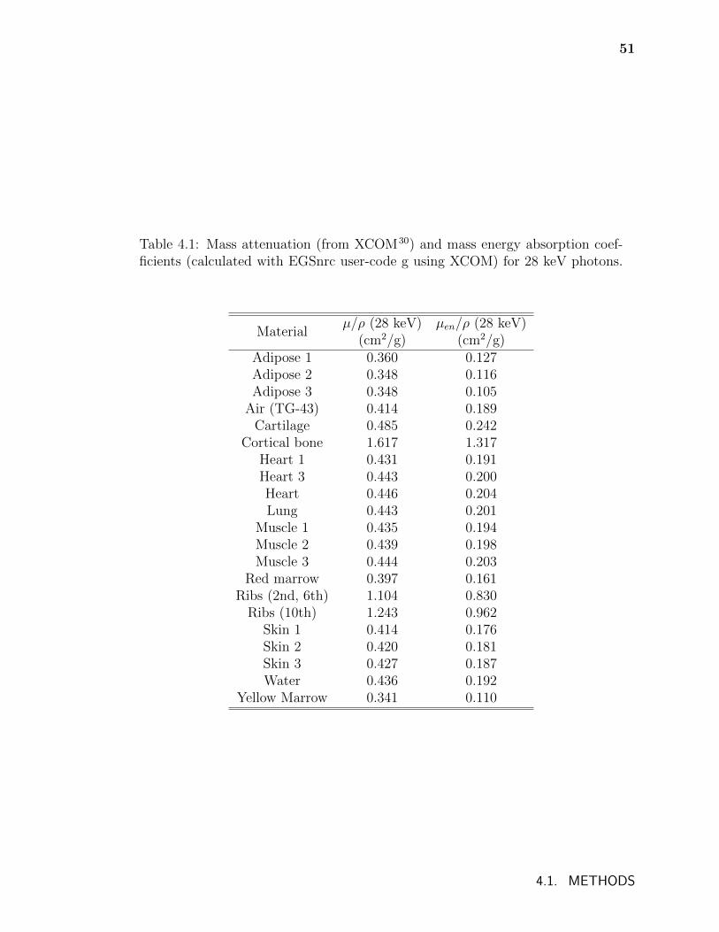
51
Table 4.1: Mass attenuation (from XCOM30) and mass energy absorption coef-ficients (calculated with EGSnrc user-code g using XCOM) for 28 keV photons.
Materialµ/ρ (28 keV) µen/ρ (28 keV)
(cm2/g) (cm2/g)Adipose 1 0.360 0.127Adipose 2 0.348 0.116Adipose 3 0.348 0.105
Air (TG-43) 0.414 0.189Cartilage 0.485 0.242
Cortical bone 1.617 1.317Heart 1 0.431 0.191Heart 3 0.443 0.200Heart 0.446 0.204Lung 0.443 0.201
Muscle 1 0.435 0.194Muscle 2 0.439 0.198Muscle 3 0.444 0.203
Red marrow 0.397 0.161Ribs (2nd, 6th) 1.104 0.830
Ribs (10th) 1.243 0.962Skin 1 0.414 0.176Skin 2 0.420 0.181Skin 3 0.427 0.187Water 0.436 0.192
Yellow Marrow 0.341 0.110
4.1. METHODS
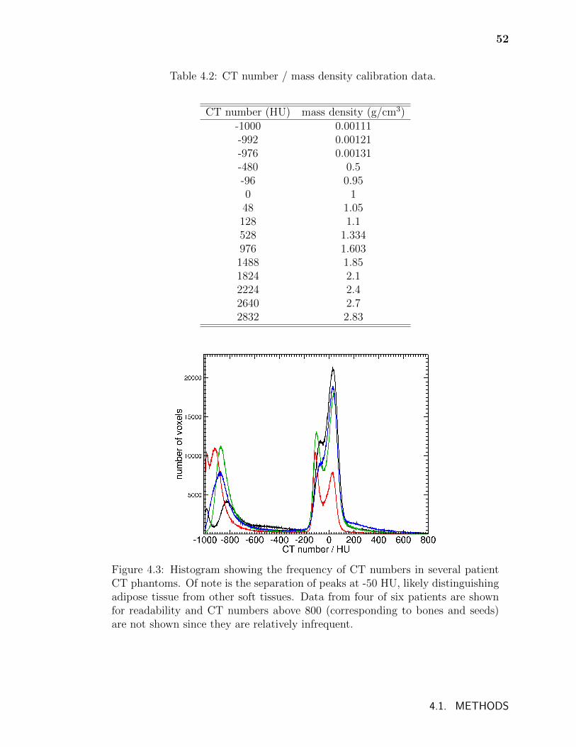
52
Table 4.2: CT number / mass density calibration data.
CT number (HU) mass density (g/cm3)-1000 0.00111-992 0.00121-976 0.00131-480 0.5-96 0.950 148 1.05128 1.1528 1.334976 1.6031488 1.851824 2.12224 2.42640 2.72832 2.83
Figure 4.3: Histogram showing the frequency of CT numbers in several patientCT phantoms. Of note is the separation of peaks at -50 HU, likely distinguishingadipose tissue from other soft tissues. Data from four of six patients are shownfor readability and CT numbers above 800 (corresponding to bones and seeds)are not shown since they are relatively infrequent.
4.1. METHODS
53
Three tissue assignment schemes of varying complexity are used and can be seen
in figure 4.4. The first scheme, denoted “detailed”, contains 20 media and includes all
tissues that may possibly be found in the CT images. Because each voxel is assigned
a tissue based on its CT number, this scheme will result in tissues in nonsensical
locations (eg. marrow outside of bones) and so illustrates the naive application of
detailed tissue assignment. The second assignment scheme, denoted “moderate”,
contains 11 media and represents a more anatomically realistic, but still fairly detailed
assignment. The three adipose tissues, each covering a reasonably large range of CT
numbers, remain separate, while other soft tissues are now assigned to muscle 2 or
heart - bloodfilled. The last scheme, denoted “simple”, contains only 5 media and
represents the traditional method of restricting the number of tissues to only a few.
The comparison of these three schemes is used to study the differences in dose and
dose metrics that occur with varying levels of tissue specificity. The differences in
dose between phantoms created with these schemes also provide an estimate of the
error that can be introduced by poor CT number to tissue conversion.
To investigate the result of an inaccurate CT number to mass density calibration,
phantoms are created that have the same tissue assignment but densities determined
by a calibration that is shifted by ±50 HU.
As the CT data do not cover the full extent of the patient, 10 cm of water is
added to every side of each phantom to ensure that the phantom extent is sufficient
to properly model photon backscatter. However, comparisons with phantoms that
lack this water padding indicate that this may not be necessary as local disagreement
only exceeds 1% within approximately 3 cm of phantom boundaries. The largest vol-
ume considered, PTV20, does not approach this region in any of the six patients and
the dose volume histograms are virtually identical for padded and non-padded phan-
toms. Tissue assignment schemes are compared using phantoms that have received
4.1. METHODS
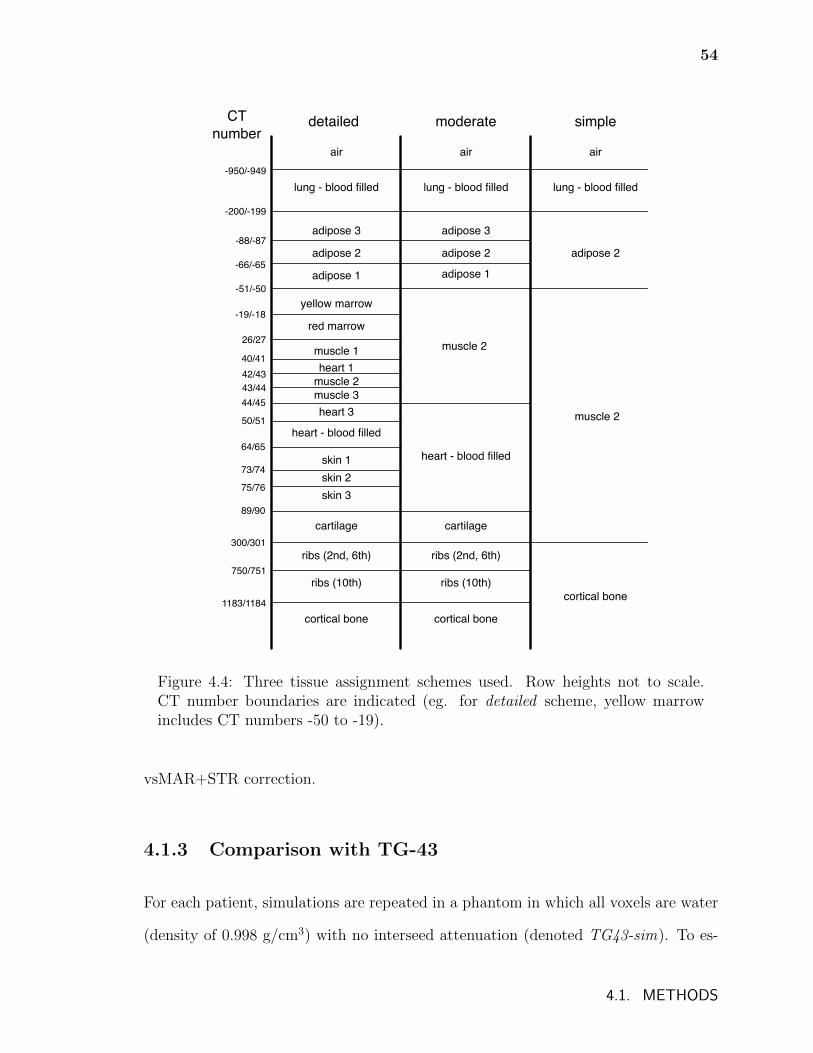
54
air air air
lung - blood filled lung - blood filled lung - blood filled
adipose 3 adipose 3
adipose 2 adipose 2 adipose 2
adipose 1 adipose 1
yellow marrow
red marrow
muscle 1
heart 1
muscle 2
muscle 3
heart 3
heart - blood filled
skin 1
skin 2
skin 3
cartilage
ribs (2nd, 6th)
ribs (10th)
cortical bone
muscle 2
heart - blood filled
cartilage
ribs (2nd, 6th)
ribs (10th)
cortical bone
muscle 2
cortical bone
-950/-949
-200/-199
-88/-87
-66/-65
-51/-50
-19/-18
26/27
40/41
42/43
43/44
44/45
50/51
64/65
73/74
75/76
89/90
300/301
750/751
1183/1184
CT
numberdetailed moderate simple
Figure 4.4: Three tissue assignment schemes used. Row heights not to scale.CT number boundaries are indicated (eg. for detailed scheme, yellow marrowincludes CT numbers -50 to -19).
vsMAR+STR correction.
4.1.3 Comparison with TG-43
For each patient, simulations are repeated in a phantom in which all voxels are water
(density of 0.998 g/cm3) with no interseed attenuation (denoted TG43-sim). To es-
4.1. METHODS
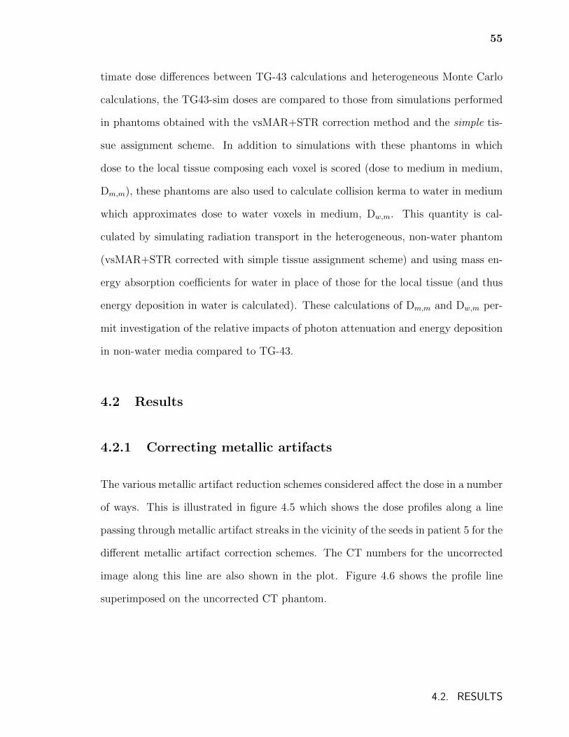
55
timate dose differences between TG-43 calculations and heterogeneous Monte Carlo
calculations, the TG43-sim doses are compared to those from simulations performed
in phantoms obtained with the vsMAR+STR correction method and the simple tis-
sue assignment scheme. In addition to simulations with these phantoms in which
dose to the local tissue composing each voxel is scored (dose to medium in medium,
Dm,m), these phantoms are also used to calculate collision kerma to water in medium
which approximates dose to water voxels in medium, Dw,m. This quantity is cal-
culated by simulating radiation transport in the heterogeneous, non-water phantom
(vsMAR+STR corrected with simple tissue assignment scheme) and using mass en-
ergy absorption coefficients for water in place of those for the local tissue (and thus
energy deposition in water is calculated). These calculations of Dm,m and Dw,m per-
mit investigation of the relative impacts of photon attenuation and energy deposition
in non-water media compared to TG-43.
4.2 Results
4.2.1 Correcting metallic artifacts
The various metallic artifact reduction schemes considered affect the dose in a number
of ways. This is illustrated in figure 4.5 which shows the dose profiles along a line
passing through metallic artifact streaks in the vicinity of the seeds in patient 5 for the
different metallic artifact correction schemes. The CT numbers for the uncorrected
image along this line are also shown in the plot. Figure 4.6 shows the profile line
superimposed on the uncorrected CT phantom.
4.2. RESULTS
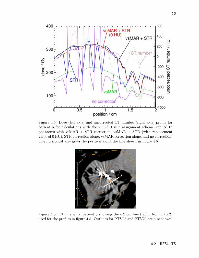
56
Figure 4.5: Dose (left axis) and uncorrected CT number (right axis) profile forpatient 5 for calculations with the simple tissue assignment scheme applied tophantoms with vsMAR + STR correction, vsMAR + STR (with replacementvalue of 0 HU), STR correction alone, vsMAR correction alone, and no correction.The horizontal axis gives the position along the line shown in figure 4.6.
Figure 4.6: CT image for patient 5 showing the ∼2 cm line (going from 1 to 2)used for the profiles in figure 4.5. Outlines for PTV05 and PTV20 are also shown.
4.2. RESULTS
57
The phantom with no correction has large spikes in dose where the CT numbers
are high enough that the voxels are assigned to cortical bone regardless of tissue
assignment scheme. Cortical bone has a high mass energy absorption coefficient: 1.317
cm2/g for 28 keV photons versus 0.201 cm2/g and 0.198 cm2/g for lung and muscle-2,
respectively. Additionally, in this uncorrected phantom, the voxels surrounding the
seeds are modelled as bone, resulting in significant attenuation of emitted photon
fluence. The dose is thus lower elsewhere in the phantom compared with all other
phantoms considered. In figure 4.5, this is illustrated in lower doses in voxels with
CT numbers below those of bone.
In the vsMAR corrected phantom, the streak artifacts are greatly reduced (see
figure 4.2b, page 49) and so the dose profile of figure 4.5 no longer passes through
bone. However, the region immediately surrounding the seeds is still modelled as
bone but now having a lower density. So while there are now no dose spikes and the
dose has increased compared to the uncorrected phantom, the dose is still lower than
that obtained by other metallic artifact reduction methods due to the attenuation of
emitted photons.
Applying the STR correction to the vsMAR corrected phantom (vsMAR+STR)
decreases the photon attenuation significantly as the seeds are no longer surrounded
by low density bone but are surrounded by lung tissue. Since the photon attenuation
is decreased, the dose increases. It is noteworthy that the dose profiles for phantoms
with replacement values of -200 HU (lung) and 0 HU (muscle) differ by only a small
amount and reflect only the difference in upstream attenuation between lung and
denser muscle.
For the phantom with only the STR correction, the dose alternates between
high and low; higher in regions where the CT numbers have been replaced with -
200 HU (lung) and lower in regions where the CT number has not been replaced
4.2. RESULTS
58
and is mostly in the range of adipose which has a significantly lower mass energy
absorption coefficient (0.116 cm2/g for 28 keV photons versus 0.201 cm2/g for lung).
The implications of the presence of adipose and muscle in the vicinity of the seeds
are discussed in section 4.3.
Table 4.3 shows the volume that receives at least the prescription dose of 100 Gy
(V100) and the minimum dose that 90% of the volume receives (D90) for PTV05, as
well as D90 for PTV20 for all six patients for the metallic artifact correction methods
discussed above. The percent difference with vsMAR+STR is also shown. As ex-
pected from figure 4.5, the vsMAR corrected phantoms and the uncorrected phantoms
have significantly lower doses than the vsMAR+STR corrected phantoms. Interest-
ingly, there is generally good agreement (differences are less than 2%) between the
vsMAR+STR corrected phantoms and the phantoms receiving only STR correction
despite the reduction of streaks with the application of vsMAR. This is due to the
fact that while significant dose differences occur in the regions of metallic artifacts,
the majority of the voxels in the PTV05 and PTV20 volumes have similar or even
equal assignments of material density and composition for the vsMAR+STR and
STR correction methods. As long as the photon fluences in the vicinity of the seeds
for the phantoms reasonably agree, the dose metrics will not differ significantly. This
is further confirmed by figure 4.7 which shows dose volume histograms for patient 1
phantoms with various correction methods for PTV05 and PTV20.
Dose metrics for phantoms with vsMAR+STR that use an STR replacement
value of 0 HU (not shown) agree with those with vsMAR+STR that use an STR
replacement value of -200 HU within approximately 2%.
4.2. RESULTS
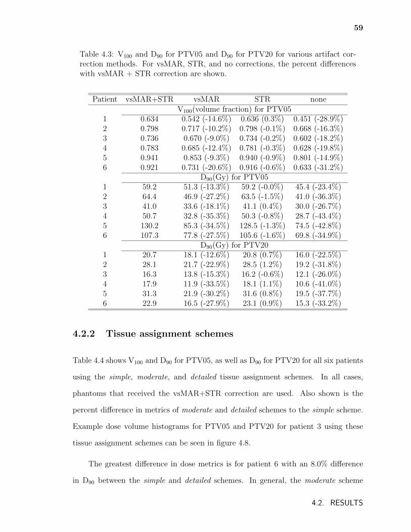
59
Table 4.3: V100 and D90 for PTV05 and D90 for PTV20 for various artifact cor-rection methods. For vsMAR, STR, and no corrections, the percent differenceswith vsMAR + STR correction are shown.
Patient vsMAR+STR vsMAR STR noneV100(volume fraction) for PTV05
1 0.634 0.542 (-14.6%) 0.636 (0.3%) 0.451 (-28.9%)2 0.798 0.717 (-10.2%) 0.798 (-0.1%) 0.668 (-16.3%)3 0.736 0.670 (-9.0%) 0.734 (-0.2%) 0.602 (-18.2%)4 0.783 0.685 (-12.4%) 0.781 (-0.3%) 0.628 (-19.8%)5 0.941 0.853 (-9.3%) 0.940 (-0.9%) 0.801 (-14.9%)6 0.921 0.731 (-20.6%) 0.916 (-0.6%) 0.633 (-31.2%)
D90(Gy) for PTV051 59.2 51.3 (-13.3%) 59.2 (-0.0%) 45.4 (-23.4%)2 64.4 46.9 (-27.2%) 63.5 (-1.5%) 41.0 (-36.3%)3 41.0 33.6 (-18.1%) 41.1 (0.4%) 30.0 (-26.7%)4 50.7 32.8 (-35.3%) 50.3 (-0.8%) 28.7 (-43.4%)5 130.2 85.3 (-34.5%) 128.5 (-1.3%) 74.5 (-42.8%)6 107.3 77.8 (-27.5%) 105.6 (-1.6%) 69.8 (-34.9%)
D90(Gy) for PTV201 20.7 18.1 (-12.6%) 20.8 (0.7%) 16.0 (-22.5%)2 28.1 21.7 (-22.9%) 28.5 (1.2%) 19.2 (-31.8%)3 16.3 13.8 (-15.3%) 16.2 (-0.6%) 12.1 (-26.0%)4 17.9 11.9 (-33.5%) 18.1 (1.1%) 10.6 (-41.0%)5 31.3 21.9 (-30.2%) 31.6 (0.8%) 19.5 (-37.7%)6 22.9 16.5 (-27.9%) 23.1 (0.9%) 15.3 (-33.2%)
4.2.2 Tissue assignment schemes
Table 4.4 shows V100 and D90 for PTV05, as well as D90 for PTV20 for all six patients
using the simple, moderate, and detailed tissue assignment schemes. In all cases,
phantoms that received the vsMAR+STR correction are used. Also shown is the
percent difference in metrics of moderate and detailed schemes to the simple scheme.
Example dose volume histograms for PTV05 and PTV20 for patient 3 using these
tissue assignment schemes can be seen in figure 4.8.
The greatest difference in dose metrics is for patient 6 with an 8.0% difference
in D90 between the simple and detailed schemes. In general, the moderate scheme
4.2. RESULTS
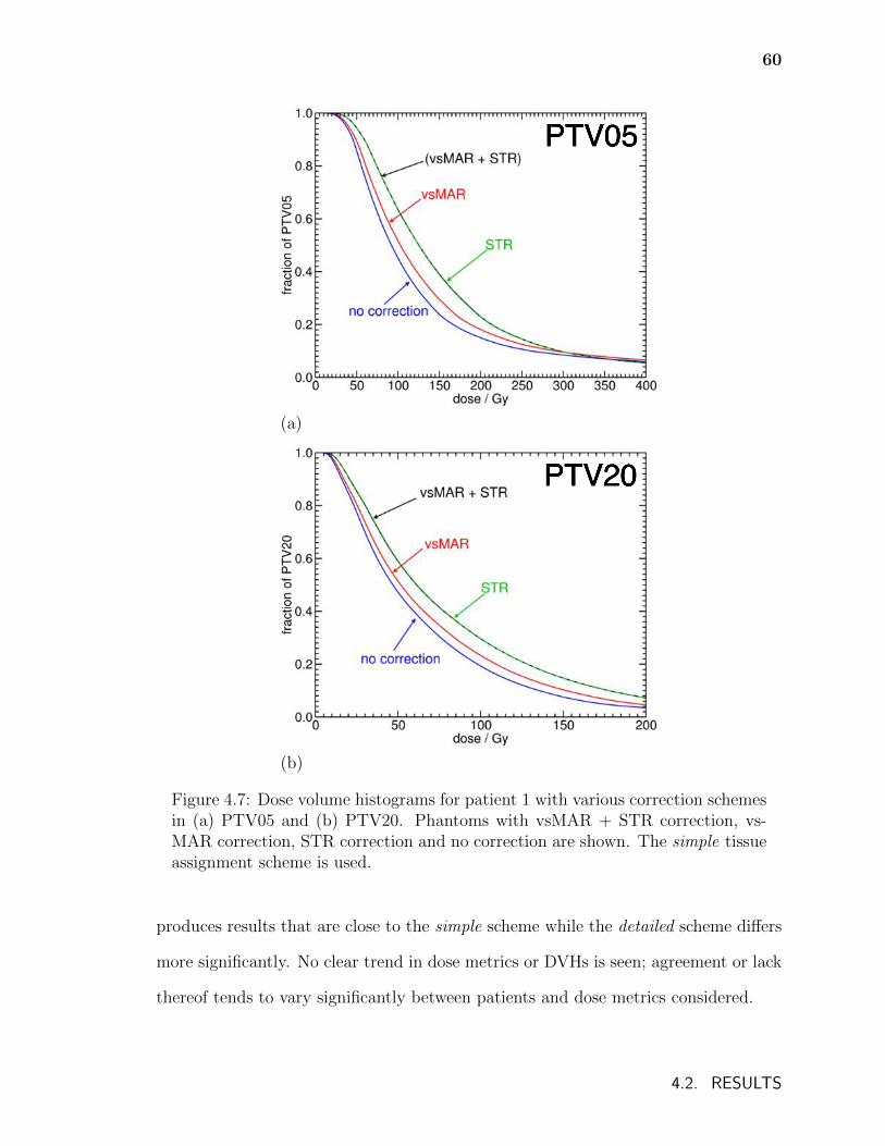
60
PTV05
(a)
PTV20
(b)
Figure 4.7: Dose volume histograms for patient 1 with various correction schemesin (a) PTV05 and (b) PTV20. Phantoms with vsMAR + STR correction, vs-MAR correction, STR correction and no correction are shown. The simple tissueassignment scheme is used.
produces results that are close to the simple scheme while the detailed scheme differs
more significantly. No clear trend in dose metrics or DVHs is seen; agreement or lack
thereof tends to vary significantly between patients and dose metrics considered.
4.2. RESULTS
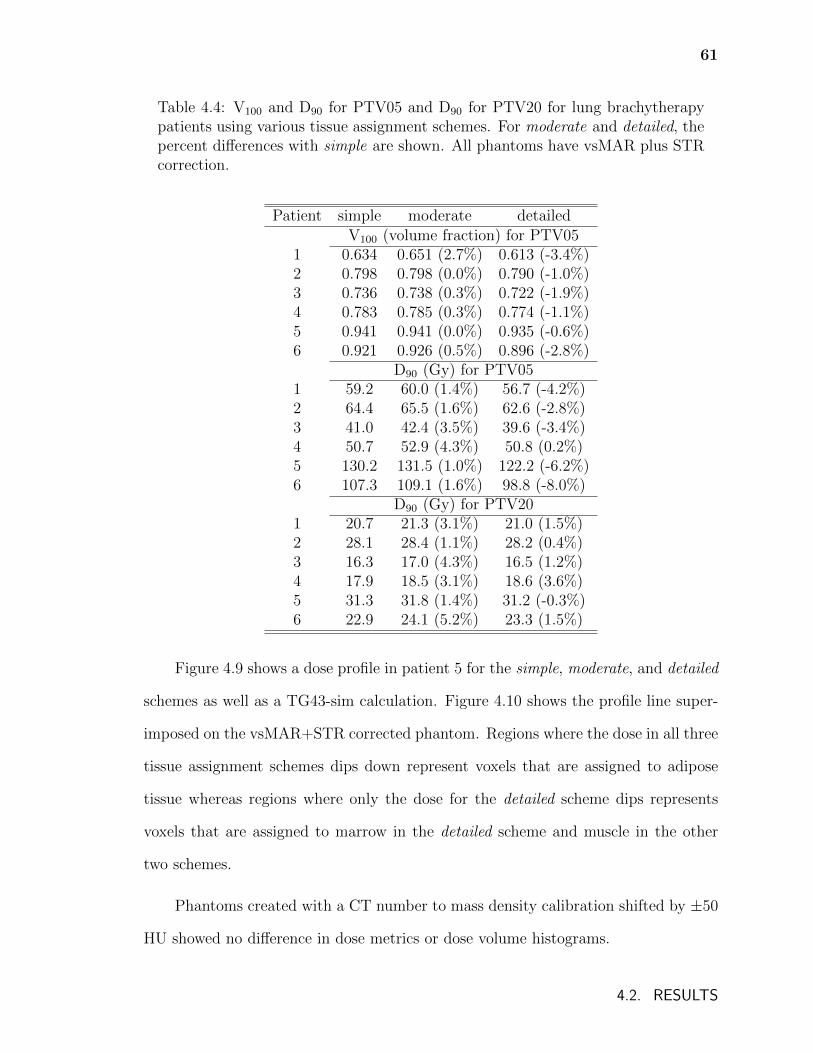
61
Table 4.4: V100 and D90 for PTV05 and D90 for PTV20 for lung brachytherapypatients using various tissue assignment schemes. For moderate and detailed, thepercent differences with simple are shown. All phantoms have vsMAR plus STRcorrection.
Patient simple moderate detailedV100 (volume fraction) for PTV05
1 0.634 0.651 (2.7%) 0.613 (-3.4%)2 0.798 0.798 (0.0%) 0.790 (-1.0%)3 0.736 0.738 (0.3%) 0.722 (-1.9%)4 0.783 0.785 (0.3%) 0.774 (-1.1%)5 0.941 0.941 (0.0%) 0.935 (-0.6%)6 0.921 0.926 (0.5%) 0.896 (-2.8%)
D90 (Gy) for PTV051 59.2 60.0 (1.4%) 56.7 (-4.2%)2 64.4 65.5 (1.6%) 62.6 (-2.8%)3 41.0 42.4 (3.5%) 39.6 (-3.4%)4 50.7 52.9 (4.3%) 50.8 (0.2%)5 130.2 131.5 (1.0%) 122.2 (-6.2%)6 107.3 109.1 (1.6%) 98.8 (-8.0%)
D90 (Gy) for PTV201 20.7 21.3 (3.1%) 21.0 (1.5%)2 28.1 28.4 (1.1%) 28.2 (0.4%)3 16.3 17.0 (4.3%) 16.5 (1.2%)4 17.9 18.5 (3.1%) 18.6 (3.6%)5 31.3 31.8 (1.4%) 31.2 (-0.3%)6 22.9 24.1 (5.2%) 23.3 (1.5%)
Figure 4.9 shows a dose profile in patient 5 for the simple, moderate, and detailed
schemes as well as a TG43-sim calculation. Figure 4.10 shows the profile line super-
imposed on the vsMAR+STR corrected phantom. Regions where the dose in all three
tissue assignment schemes dips down represent voxels that are assigned to adipose
tissue whereas regions where only the dose for the detailed scheme dips represents
voxels that are assigned to marrow in the detailed scheme and muscle in the other
two schemes.
Phantoms created with a CT number to mass density calibration shifted by ±50
HU showed no difference in dose metrics or dose volume histograms.
4.2. RESULTS
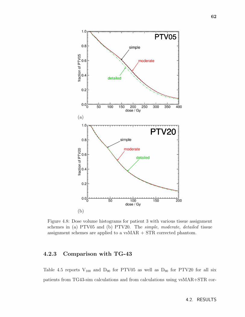
62
PTV05
(a)
PTV20
(b)
Figure 4.8: Dose volume histograms for patient 3 with various tissue assignmentschemes in (a) PTV05 and (b) PTV20. The simple, moderate, detailed tissueassignment schemes are applied to a vsMAR + STR corrected phantom.
4.2.3 Comparison with TG-43
Table 4.5 reports V100 and D90 for PTV05 as well as D90 for PTV20 for all six
patients from TG43-sim calculations and from calculations using vsMAR+STR cor-
4.2. RESULTS
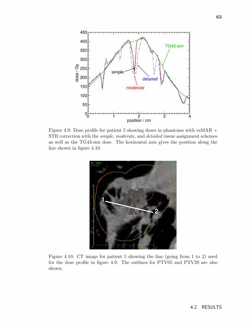
63
Figure 4.9: Dose profile for patient 5 showing doses in phantoms with vsMAR +STR correction with the simple, moderate, and detailed tissue assignment schemesas well as the TG43-sim dose. The horizontal axis gives the position along theline shown in figure 4.10.
Figure 4.10: CT image for patient 5 showing the line (going from 1 to 2) usedfor the dose profile in figure 4.9. The outlines for PTV05 and PTV20 are alsoshown.
4.2. RESULTS
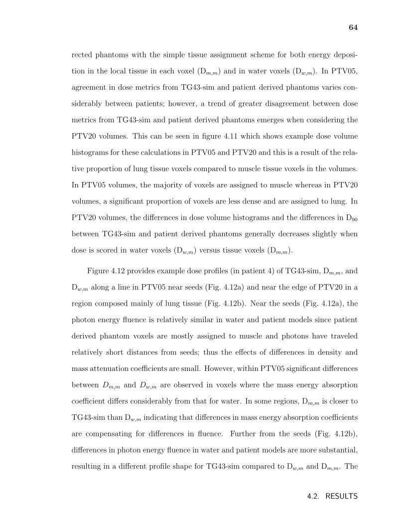
64
rected phantoms with the simple tissue assignment scheme for both energy deposi-
tion in the local tissue in each voxel (Dm,m) and in water voxels (Dw,m). In PTV05,
agreement in dose metrics from TG43-sim and patient derived phantoms varies con-
siderably between patients; however, a trend of greater disagreement between dose
metrics from TG43-sim and patient derived phantoms emerges when considering the
PTV20 volumes. This can be seen in figure 4.11 which shows example dose volume
histograms for these calculations in PTV05 and PTV20 and this is a result of the rela-
tive proportion of lung tissue voxels compared to muscle tissue voxels in the volumes.
In PTV05 volumes, the majority of voxels are assigned to muscle whereas in PTV20
volumes, a significant proportion of voxels are less dense and are assigned to lung. In
PTV20 volumes, the differences in dose volume histograms and the differences in D90
between TG43-sim and patient derived phantoms generally decreases slightly when
dose is scored in water voxels (Dw,m) versus tissue voxels (Dm,m).
Figure 4.12 provides example dose profiles (in patient 4) of TG43-sim, Dm,m, and
Dw,m along a line in PTV05 near seeds (Fig. 4.12a) and near the edge of PTV20 in a
region composed mainly of lung tissue (Fig. 4.12b). Near the seeds (Fig. 4.12a), the
photon energy fluence is relatively similar in water and patient models since patient
derived phantom voxels are mostly assigned to muscle and photons have traveled
relatively short distances from seeds; thus the effects of differences in density and
mass attenuation coefficients are small. However, within PTV05 significant differences
between Dm,m and Dw,m are observed in voxels where the mass energy absorption
coefficient differs considerably from that for water. In some regions, Dm,m is closer to
TG43-sim than Dw,m indicating that differences in mass energy absorption coefficients
are compensating for differences in fluence. Further from the seeds (Fig. 4.12b),
differences in photon energy fluence in water and patient models are more substantial,
resulting in a different profile shape for TG43-sim compared to Dw,m and Dm,m. The
4.2. RESULTS
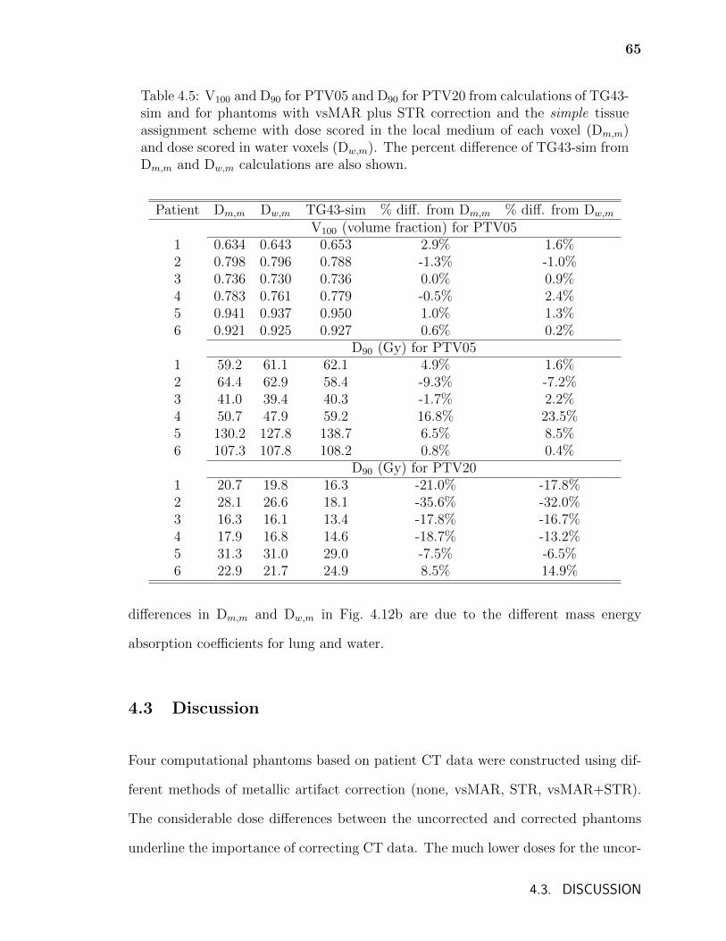
65
Table 4.5: V100 and D90 for PTV05 and D90 for PTV20 from calculations of TG43-sim and for phantoms with vsMAR plus STR correction and the simple tissueassignment scheme with dose scored in the local medium of each voxel (Dm,m)and dose scored in water voxels (Dw,m). The percent difference of TG43-sim fromDm,m and Dw,m calculations are also shown.
Patient Dm,m Dw,m TG43-sim % diff. from Dm,m % diff. from Dw,m
V100 (volume fraction) for PTV051 0.634 0.643 0.653 2.9% 1.6%2 0.798 0.796 0.788 -1.3% -1.0%3 0.736 0.730 0.736 0.0% 0.9%4 0.783 0.761 0.779 -0.5% 2.4%5 0.941 0.937 0.950 1.0% 1.3%6 0.921 0.925 0.927 0.6% 0.2%
D90 (Gy) for PTV051 59.2 61.1 62.1 4.9% 1.6%2 64.4 62.9 58.4 -9.3% -7.2%3 41.0 39.4 40.3 -1.7% 2.2%4 50.7 47.9 59.2 16.8% 23.5%5 130.2 127.8 138.7 6.5% 8.5%6 107.3 107.8 108.2 0.8% 0.4%
D90 (Gy) for PTV201 20.7 19.8 16.3 -21.0% -17.8%2 28.1 26.6 18.1 -35.6% -32.0%3 16.3 16.1 13.4 -17.8% -16.7%4 17.9 16.8 14.6 -18.7% -13.2%5 31.3 31.0 29.0 -7.5% -6.5%6 22.9 21.7 24.9 8.5% 14.9%
differences in Dm,m and Dw,m in Fig. 4.12b are due to the different mass energy
absorption coefficients for lung and water.
4.3 Discussion
Four computational phantoms based on patient CT data were constructed using dif-
ferent methods of metallic artifact correction (none, vsMAR, STR, vsMAR+STR).
The considerable dose differences between the uncorrected and corrected phantoms
underline the importance of correcting CT data. The much lower doses for the uncor-
4.3. DISCUSSION
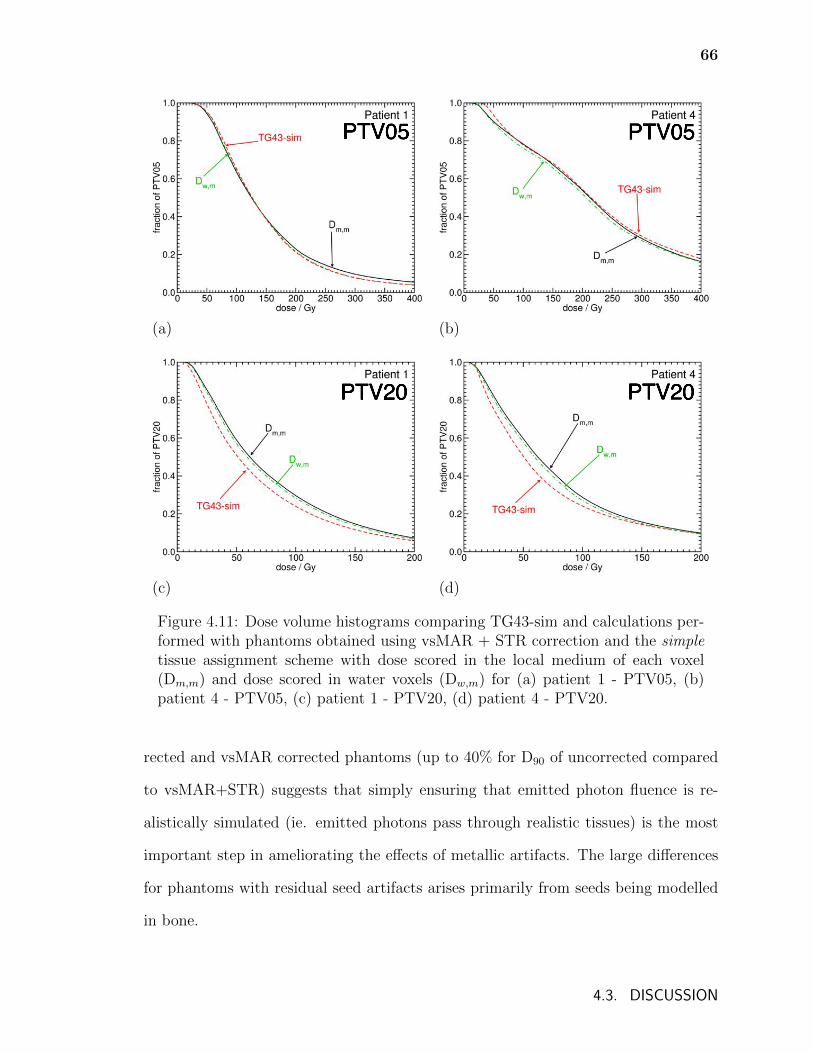
66
PTV05 PTV05
(a) (b)
PTV20 PTV20
(c) (d)
Figure 4.11: Dose volume histograms comparing TG43-sim and calculations per-formed with phantoms obtained using vsMAR + STR correction and the simpletissue assignment scheme with dose scored in the local medium of each voxel(Dm,m) and dose scored in water voxels (Dw,m) for (a) patient 1 - PTV05, (b)patient 4 - PTV05, (c) patient 1 - PTV20, (d) patient 4 - PTV20.
rected and vsMAR corrected phantoms (up to 40% for D90 of uncorrected compared
to vsMAR+STR) suggests that simply ensuring that emitted photon fluence is re-
alistically simulated (ie. emitted photons pass through realistic tissues) is the most
important step in ameliorating the effects of metallic artifacts. The large differences
for phantoms with residual seed artifacts arises primarily from seeds being modelled
in bone.
4.3. DISCUSSION
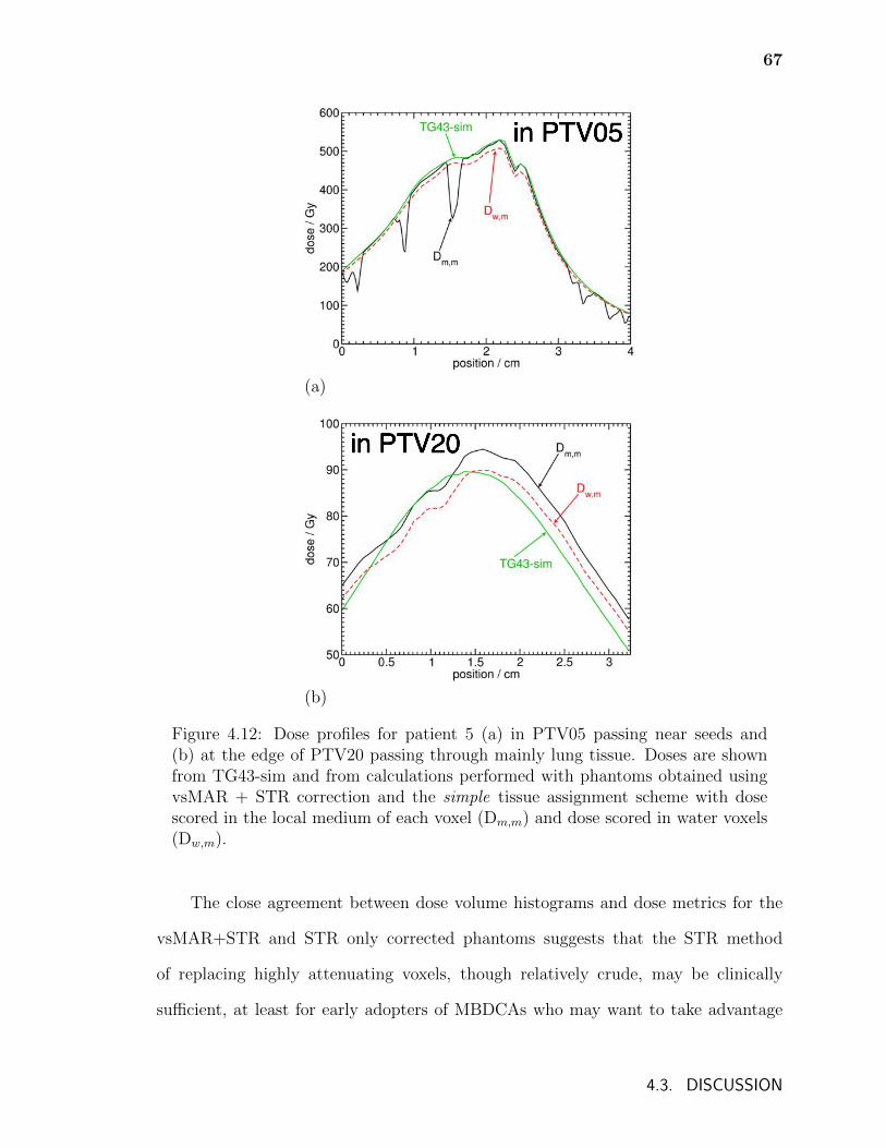
67
in PTV05
(a)
in PTV20
(b)
Figure 4.12: Dose profiles for patient 5 (a) in PTV05 passing near seeds and(b) at the edge of PTV20 passing through mainly lung tissue. Doses are shownfrom TG43-sim and from calculations performed with phantoms obtained usingvsMAR + STR correction and the simple tissue assignment scheme with dosescored in the local medium of each voxel (Dm,m) and dose scored in water voxels(Dw,m).
The close agreement between dose volume histograms and dose metrics for the
vsMAR+STR and STR only corrected phantoms suggests that the STR method
of replacing highly attenuating voxels, though relatively crude, may be clinically
sufficient, at least for early adopters of MBDCAs who may want to take advantage
4.3. DISCUSSION
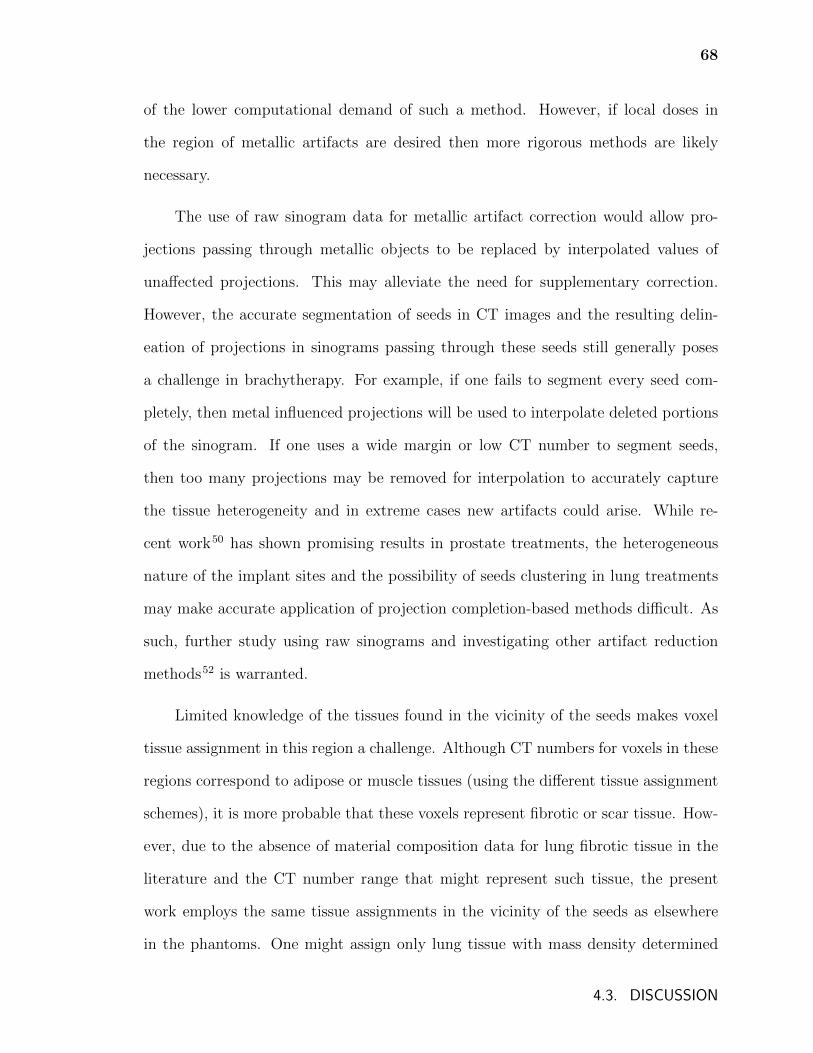
68
of the lower computational demand of such a method. However, if local doses in
the region of metallic artifacts are desired then more rigorous methods are likely
necessary.
The use of raw sinogram data for metallic artifact correction would allow pro-
jections passing through metallic objects to be replaced by interpolated values of
unaffected projections. This may alleviate the need for supplementary correction.
However, the accurate segmentation of seeds in CT images and the resulting delin-
eation of projections in sinograms passing through these seeds still generally poses
a challenge in brachytherapy. For example, if one fails to segment every seed com-
pletely, then metal influenced projections will be used to interpolate deleted portions
of the sinogram. If one uses a wide margin or low CT number to segment seeds,
then too many projections may be removed for interpolation to accurately capture
the tissue heterogeneity and in extreme cases new artifacts could arise. While re-
cent work50 has shown promising results in prostate treatments, the heterogeneous
nature of the implant sites and the possibility of seeds clustering in lung treatments
may make accurate application of projection completion-based methods difficult. As
such, further study using raw sinograms and investigating other artifact reduction
methods52 is warranted.
Limited knowledge of the tissues found in the vicinity of the seeds makes voxel
tissue assignment in this region a challenge. Although CT numbers for voxels in these
regions correspond to adipose or muscle tissues (using the different tissue assignment
schemes), it is more probable that these voxels represent fibrotic or scar tissue. How-
ever, due to the absence of material composition data for lung fibrotic tissue in the
literature and the CT number range that might represent such tissue, the present
work employs the same tissue assignments in the vicinity of the seeds as elsewhere
in the phantoms. One might assign only lung tissue with mass density determined
4.3. DISCUSSION
69
by voxel CT numbers in the vicinity of the seeds but there is no evidence that the
composition of fibrotic tissue is closer to that of healthy lung than to muscle or other
tissues. Fibrotic tissues or mixtures of lung and fibrotic tissues might cover a wide
range of CT numbers. Regardless, since there is a degeneracy of tissue parameters for
a given CT number, and the elemental composition of fibrotic tissue is unknown, the
assignment of any tissue is still somewhat arbitrary and represents an uncertainty.
The sensitivity of dose distributions on the modelling of fibrotic tissue is an issue that
is approached in chapter 5.
The effect of different tissue assignment schemes on dose varies from patient to
patient. The varied nature of the differences that can arise emphasizes the need for
a rigorous and accurate method of assigning material compositions. The use of dual
energy CT108 or other novel methods may be required to determine voxel parameters.
Additionally, the uncertainty of the elemental composition of tissues themselves is
unclear and more study of tissue composition is required.
This uncertainty in tissue assignment means that absolute comparisons with TG-
43 doses in the immediate vicinity of the seeds (PTV05) should be undertaken with
caution. However, it is possible to conclude that in volumes that contain a signifi-
cant amount of healthy lung tissue, TG-43 calculations are likely to underestimate
the dose by as much as 35%. Compared to water, lung tissue has a higher mass
energy absorption coefficient (approximately 4.7% difference for 28 keV photons), a
lower density, and a relatively similar mass attenuation coefficient (approximately
1.6% difference for 28 keV photons); lung voxels will attenuate photon fluence less
while simultaneously absorbing more dose than water. Thus, the more healthy lung
a volume contains, the more TG-43 will underestimate dose as illustrated in table
4.5 and figures 4.11 and 4.12. For the patient data sets considered, scoring energy
deposition in water voxels (Dw,m) rather than in the local tissue (Dm,m) does not gen-
4.3. DISCUSSION
70
erally improve agreement with TG-43 calculated doses; only a small change in percent
difference of D90 between TG43-sim and model-based doses is seen in PTV20. This
implies that for volumes containing greater proportions of lung tissue, discrepancies
between TG-43 and model-based doses are mainly due to differences in calculated
photon energy fluence.
Beyond the issues already discussed, there remain a number of unanswered ques-
tions that are relevant to using MBDCAs for lung brachytherapy dosimetry. The
most immediate are related to the accuracy of using CT data from a snapshot in
time to calculate the dose that is absorbed by the patient over weeks. Seed positions
may change with time as air kerma strength diminishes, affecting doses delivered.
The effects of breathing motion on patient dosimetry is probably much lower than for
external beam treatments; this has been studied for 192Ir bile duct implants109 but
not for 125I lung implants. Additionally, the tissue composition in the patient is likely
to change as fibrotic and scar tissue develops and swelling subsides following surgery.
In the future, MBDCAs will be instrumental in assessing the impact of these effects
on doses delivered.
4.4 Conclusions
Full Monte Carlo calculations were performed for six 125I lung brachytherapy patients
treated at the Mayo Clinic Rochester using BrachyDose. Different metallic artifact
and tissue assignment schemes were considered and their effects on dose distributions
were investigated.
Large differences between phantoms that receive metallic artifact correction and
no correction underline the necessity of mitigation of the effects of metallic artifacts
for MBDCAs for lung brachytherapy. The agreement in DVHs and dose metrics be-
4.4. CONCLUSIONS
71
tween phantoms receiving vsMAR+STR and STR corrections suggest that simpler
correction methods may be clinically sufficient providing they correct for voxels that
would otherwise cause unrealistically high attenuation of emitted photon fluence. The
challenges posed by seed artifacts found in these patients motivates further investi-
gation of metallic artifact reduction schemes for lung brachytherapy in chapter 5.
The three different tissue assignment schemes used resulted in disagreement in
dose metrics that varied unpredictably for each patient. This suggests that a rigor-
ous and accurate method of determining voxel parameters and tissue assignment is
necessary. However, results suggest that patient dose is insensitive to small errors in
assigning mass density assuming elemental composition remains constant. A source
of uncertainty is the composition of the tissue in the vicinity of the seeds which may
be lung fibrotic tissue (see chapter 5). Rigorous implementation of MBDCAs may
require knowledge of the elemental composition of this tissue.
Despite the uncertainties introduced with MBDCAs, significant differences in
DVHs and dose metrics between MBDCAs and TG-43 are likely. Generally, TG-43
calculations underestimate doses in volumes containing significant amounts of healthy
lung tissue.
4.4. CONCLUSIONS

Chapter 5
Metallic artifact mitigation and
organ-constrained tissue assignment for
lung brachytherapy
As a continuation of the previous chapter which identified the salient modelling is-
sues, this chapter presents an investigation of improved techniques for the accurate
calculation of permanent implant lung brachytherapy dose distributions. Specifically,
this chapter seeks methods to improve the accuracy of CT-derived computational
phantoms by further examining the issue of metallic artifact reduction as well as
investigating the practice of constraining tissue assignments within organ contours.
The investigation of metallic artifact reduction techniques is continued by com-
paring three techniques: the simple threshold replacement technique of chapter 4, a
technique involving the filtered back projection of a modified virtual sinogram (an
improvement on the vsMAR technique), and a 3D adaptive median filter technique52.
Before accurately assigning discrete tissues from CT numbers, two challenges
must be addressed: a number of human tissues are poorly distinguished by CT number
with multiple tissues of differing atomic composition corresponding to the same CT
number44 and voxel CT numbers may correspond to tissues that are anatomically
erroneous, particularly in heterogeneous regions such as the lung, due to noise, scatter,
72
73
and voxel volume averaging in CT imaging. Additionally, the presence of fibrotic
tissue of unknown atomic composition in lung brachytherapy patients is a source of
unresolved uncertainty.
The report of Task Group 186 on model-based dose calculation methods in
brachytherapy beyond the TG-43 formalism29 recommends that the assignment of
tissues be guided by organ contours. Organ-constrained tissue assignment has been
shown to affect dose distributions in external beam radiotherapy where dose is less
sensitive to atomic composition110. By applying separate tissue assignment schemes
within organ contours, the mis-assignment of tissues may be reduced and the effect
of incomplete artifact correction may be minimized. While organ-constrained tis-
sue assignment schemes may resolve some problems in the assignment of elemental
compositions to voxels in computational phantoms, it does not address the incorrect
assignment of voxel density due to metallic artifacts. The TG-186 report recom-
mends that if metallic artifacts are present, the density of the tissue in question be
over-ridden.
This chapter uses Monte Carlo simulations and data from the lung brachytherapy
patients of chapter 4 to investigate metallic artifact mitigation and tissue assignment
by calculating dose distributions for a variety of computational phantom models.
Computational phantoms are generated from uncorrected CT images as well as CT
images on which different metallic artifact reduction techniques have been applied.
Tissue assignment schemes are applied both globally or constrained within lung con-
tours. Voxel densities are assigned using a CT number to density calibration or using
the nominal density of the voxel tissue. Phantoms with muscle tissue assigned within
lung contours are used to investigate the magnitude of dose differences that might
arise due to the presence of fibrotic tissue (composition unknown).
74
5.1 Methods
5.1.1 Metallic artifact reduction
The patient CT images of chapter 4 are treated with three metallic artifact reduction
techniques. The first method is the “simple threshold replacement” method presented
in chapter 4 (page 48). The second method, a fan beam virtual sinogram method
labeled “fan”, is an improved version of the method used in the previous chapter: in
lieu of the radon transform used previously, a built-in MATLAB (The Mathworks,
Natick Mass. USA) fan-beam transform is used to create a virtual sinogram. A
threshold of 1500 HU is used to delineate segments of the original image correspond-
ing to metallic seeds. Portions of the virtual sinogram corresponding to projections
passing through the seeds are deleted and replaced with cubic spline interpolations
of adjacent projections. A filtered back-projection is then performed using an inverse
fan beam transform on the resulting virtual sinogram to produce the corrected image.
For the fan beam transform, an arc sensor geometry is used with a sensor spacing
of 0.1 degrees and a rotation increment of 0.1 degrees. The distance in pixels from
the fan-beam vertex to the centre of rotation is determined using the distance from
source to detector and pixel sizes defined in the CT image meta-information. While
the “fan” technique leaves fewer residual artifacts compared to the vsMAR method of
chapter 4, some residual artifacts still remain in the immediate vicinity of the sources
and so dose calculations are performed with phantoms generated from CT images
that receive the “fan” method alone as well as those that receive “fan” followed by
STR to help further eliminate these residual artifacts.
The third technique, labeled “median”, is a 3D adaptive median filter based on
the work of Basran et al.52 but differs slightly since our aim is to remove both metal
5.1. METHODS
75
streak artifacts and 125I seeds because BrachyDose models the seeds separately. To
ensure that seeds are removed from CT images, a 30 bin histogram of the frequency
of CT numbers in the image is created. Any voxel with a CT number greater than
1500 HU is replaced with the CT number that corresponds to the greatest histogram
bin that has at least 10% of image voxels. Next, a region of interest (ROI) of 5 x 5 x 7
voxels is defined around each voxel and two filters are applied. In the first filter,
the median CT number and standard deviation of the ROI is calculated and if the
voxel CT number is greater or less than 0.25 times the standard deviation from the
median value in the ROI, it is replaced by the adjacent voxel value in one of the two
neighbouring slices that is nearest to the median. To reduce noise introduced by the
first filter, a second filter is applied where the median value of the 3D ROI is computed
and replaces each voxel value. The 3D ROI size is chosen so as to enhance artifact
reduction while reducing loss of soft tissue detail and other algorithm parameters are
chosen for effectiveness.
Table 5.1 summarizes the labels and descriptions of the metallic artifact reduction
techniques.
5.1.2 Tissue assignment schemes and development of
computational phantoms
Phantoms from three representative patients (patients 1,2 and 5) from chapter 4 are
chosen for dose calculations. In each case, CT images are resampled to a maximum
of 300 voxels in each direction for computational efficiency before being converted to
EGSnrc phantom files (.egsphant). Tissue assignment schemes are created consisting
of air, lung, adipose, muscle, and cortical bone. Tissue compositions taken from
Woodard and White85 are given in table 2.1 (page 19).
5.1. METHODS

76
Table 5.1: Summary of metallic artifact reduction techniques
Label Descriptionuncorr. Original, uncorrected CT imageSTR Simple threshold replacement: Within a 1x1x1cm3 cube cen-
tred around each seed position, if a voxel CT number isgreater than or equal to 88 HU, it is replaced with a CTnumber of -200 HU.
fan Fan beam virtual sinogram: A fan beam transform is usedto create a virtual sinogram. Projections passing throughvoxels with CT numbers greater than or equal to 1500 HU aredeleted and replaced with spline interpolations of surroundingprojections. A filtered back projection is performed using aninverse fan beam transform to recreate the image.
median Median filter: Each voxel value is compared with a 3D localmedian value and replaced with an adjacent voxel value if itdiffers by 0.25 times the standard deviation. A second filteris used to smooth the image.
Four tissue assignment schemes are used to generate computational phantoms
from uncorrected and corrected CT images and are represented in figure 5.1. The
first assignment scheme is labeled “unconstrained” and is assigned globally. The
second assignment scheme, labeled “lung, air” is identical to “unconstrained” except
inside lung contours where only lung and air are assigned. The third scheme, “lung,
air, muscle” is similar to “lung, air” but allows the assignment of muscle tissue to
approximately investigate the effect of the fibrotic tissue of unknown composition
(as fibrotic tissue may form in the vicinity of the implant following surgery). For
“unconstrained”, “lung, air”, and “lung, air, muscle”, the mass density of each voxel
is determined by the CT number to mass density calibration in table 4.2. The last
scheme, “lung, air (nominal)” has the same tissue assignment as “lung, air” but,
throughout the phantom, voxel densities are defined as the nominal density of the
local voxel tissue. The tissue assignment schemes of this chapter are based on the
“simple” scheme of chapter 4: the CT number boundaries between tissues represent a
5.1. METHODS
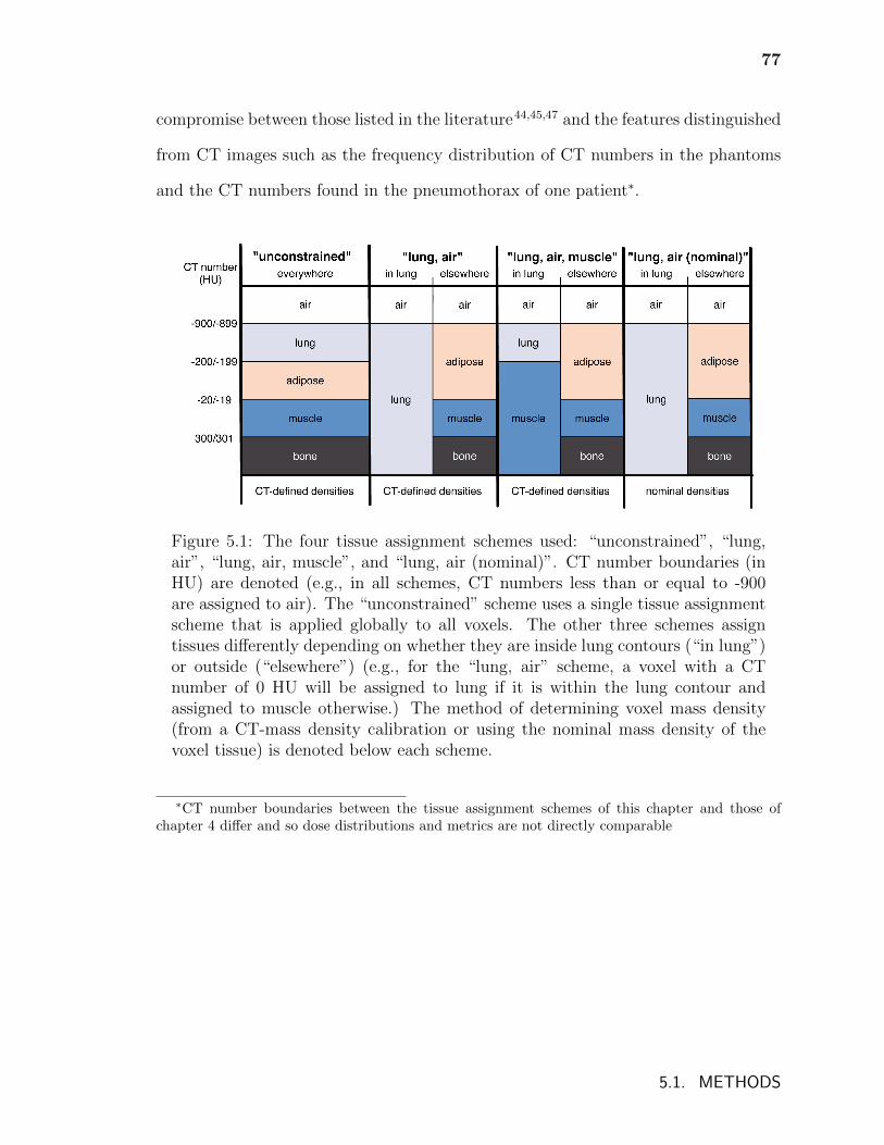
77
compromise between those listed in the literature44,45,47 and the features distinguished
from CT images such as the frequency distribution of CT numbers in the phantoms
and the CT numbers found in the pneumothorax of one patient∗.
Figure 5.1: The four tissue assignment schemes used: “unconstrained”, “lung,air”, “lung, air, muscle”, and “lung, air (nominal)”. CT number boundaries (inHU) are denoted (e.g., in all schemes, CT numbers less than or equal to -900are assigned to air). The “unconstrained” scheme uses a single tissue assignmentscheme that is applied globally to all voxels. The other three schemes assigntissues differently depending on whether they are inside lung contours (“in lung”)or outside (“elsewhere”) (e.g., for the “lung, air” scheme, a voxel with a CTnumber of 0 HU will be assigned to lung if it is within the lung contour andassigned to muscle otherwise.) The method of determining voxel mass density(from a CT-mass density calibration or using the nominal mass density of thevoxel tissue) is denoted below each scheme.
∗CT number boundaries between the tissue assignment schemes of this chapter and those ofchapter 4 differ and so dose distributions and metrics are not directly comparable
5.1. METHODS
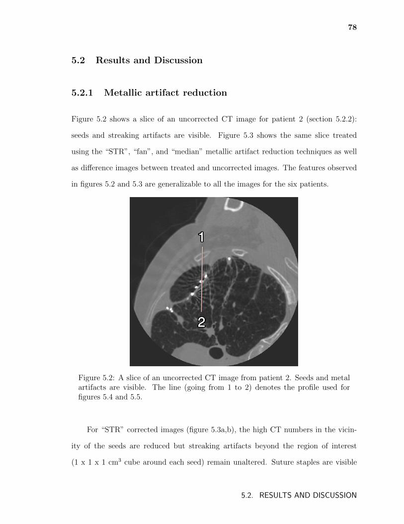
78
5.2 Results and Discussion
5.2.1 Metallic artifact reduction
Figure 5.2 shows a slice of an uncorrected CT image for patient 2 (section 5.2.2):
seeds and streaking artifacts are visible. Figure 5.3 shows the same slice treated
using the “STR”, “fan”, and “median” metallic artifact reduction techniques as well
as difference images between treated and uncorrected images. The features observed
in figures 5.2 and 5.3 are generalizable to all the images for the six patients.
Figure 5.2: A slice of an uncorrected CT image from patient 2. Seeds and metalartifacts are visible. The line (going from 1 to 2) denotes the profile used forfigures 5.4 and 5.5.
For “STR” corrected images (figure 5.3a,b), the high CT numbers in the vicin-
ity of the seeds are reduced but streaking artifacts beyond the region of interest
(1 x 1 x 1 cm3 cube around each seed) remain unaltered. Suture staples are visible
5.2. RESULTS AND DISCUSSION
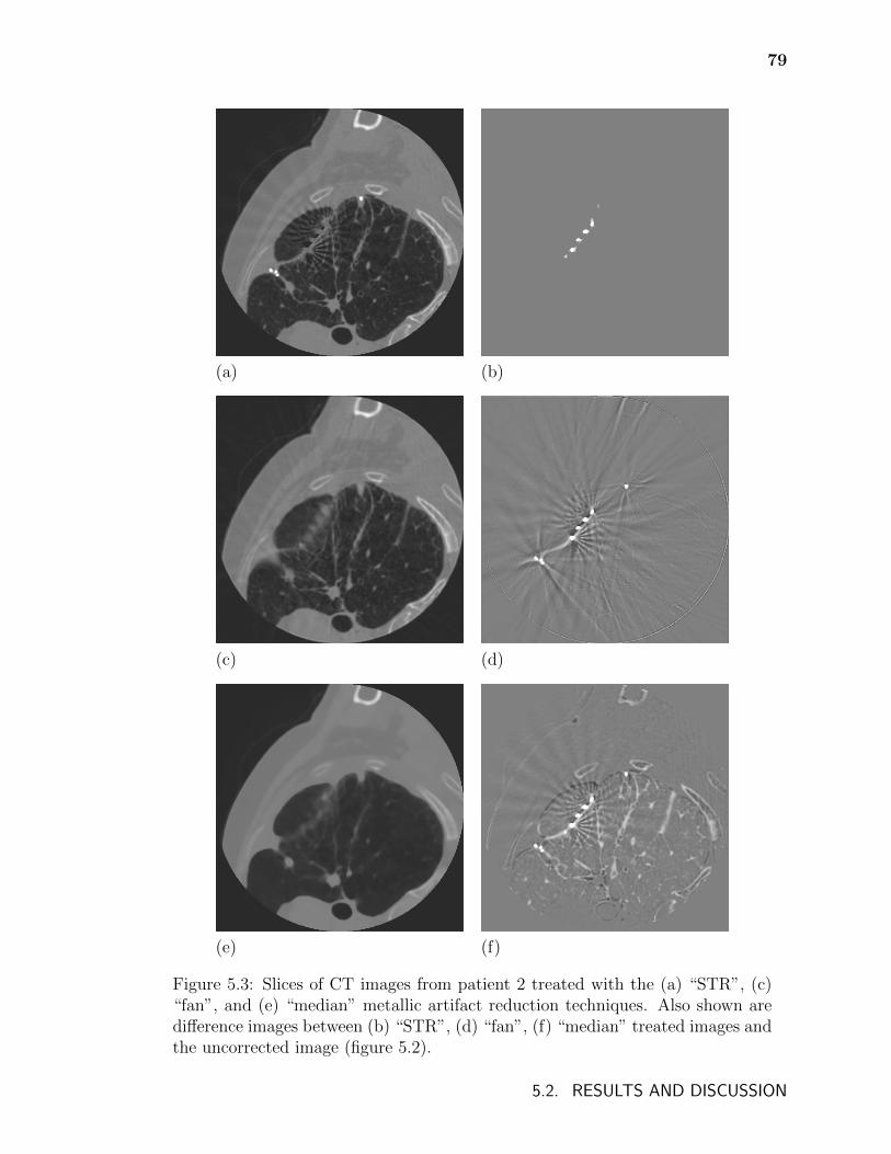
79
(a) (b)
(c) (d)
(e) (f)
Figure 5.3: Slices of CT images from patient 2 treated with the (a) “STR”, (c)“fan”, and (e) “median” metallic artifact reduction techniques. Also shown aredifference images between (b) “STR”, (d) “fan”, (f) “median” treated images andthe uncorrected image (figure 5.2).
5.2. RESULTS AND DISCUSSION
80
in figure 5.3 (a) and may cause mis-assignment of tissues since metal is not included
in tissue assignment schemes. However, the staples are small and are not likely to
considerably affect dose. Since the algorithm is only applied in the vicinity of the
seeds, elsewhere, soft tissue and bone details from the original image remains intact.
For “fan” corrected images (figure 5.3c,d), high CT numbers due to seeds and
staples as well as metallic streaking artifacts are reduced; however, some residual
artifacts remain and are observed as subtle streaks in figure 5.3c. Soft tissue and bone
details are preserved. Since projections that pass near but not through seeds are used
for the spline interpolations in the virtual sinograms, interpolations are calculated
using data that has itself been affected by streaking artifacts, possibly contributing
to the residual artifacts. Metallic artifacts are more severe in the immediate vicinity
of the seeds and so one might consider adding a margin to voxels corresponding to
seed positions when delineating projections in virtual sinograms that correspond to
seeds. This would mean that interpolations over deleted segments of virtual sinograms
are performed using data that is less affected by artifacts but over a larger gap of
missing data. Selecting the projections in virtual sinograms to delete and replace
with interpolations, either by adjusting the CT number threshold that corresponds
to seeds or by adding margins around detected seeds, requires finding a balance:
if deleted segments are too large then interpolation breaks down and new artifacts
are created, however, smaller deletions leave existing artifacts and high CT numbers
uncorrected. Access to original sinogram data might make this balance easier to
achieve as projections passing near but not through seeds are less likely to be affected
by metallic artifacts in original sinograms. However, it is unclear whether any benefit
gained from using original sinogram data would justify the greater complexity of
adopting such an approach clinically.
For “median” corrected images (figure 5.3e,f), high CT numbers due to seeds
5.2. RESULTS AND DISCUSSION
81
and metallic streaking artifacts are reduced with no residual artifacts visible. Suture
staples are also removed. However, while the second smoothing filter reduces noise, it
also impacts some of the heterogeneities present in the images. This is most apparent
in the loss of detail in the lung as well as a reduction of intensity in ribs. The
median filter method introduced by Basran et al.52 uses a CT number threshold of
2000 HU above which voxels are left unchanged. This is to preserve CT numbers that
correspond to bone and seeds. However, our goal is to remove seeds from CT images
so that they can be modelled separately by BrachyDose, and so the use of such a
threshold is inappropriate. Basran et al. also discuss how the median filter reduces
contrast within regions with a large range of CT intensities and suggest modifying
the filter to ignore voxels with very low CT numbers and CT numbers corresponding
to bone. Unfortunately, since lung brachytherapy implants are found in regions with
large ranges of CT number, such an approach would greatly reduce the ability of the
median filter to reduce metallic artifacts in the images used in this study.
For each of the images shown in figures 5.2 (page 78) and 5.3 (page 79), figure 5.4a
presents the CT number profile along the line shown in figure 5.2, while figure 5.4b
displays the tissue that would be assigned along that profile if the “unconstrained” tis-
sue assignment were used for each slice. All three metallic artifact reduction schemes
reduce the high CT numbers associated with the seed at approximately 4 cm. Beyond
this region, the CT numbers for the “STR” treated image exactly match those for
the uncorrected image. As a result, the unmitigated streaking artifacts seen between
4 and 7 cm result in the erroneous assignment of voxels to air and adipose for these
two images. Both “fan” and “median” treated profiles reduce high CT numbers due
to seeds and streaking artifacts sufficiently such that lung tissue is properly assigned
although the density assigned along the profiles would differ between the two. The
two peaks in CT number at approximately 1 cm corresponding to a rib are not fully
5.2. RESULTS AND DISCUSSION
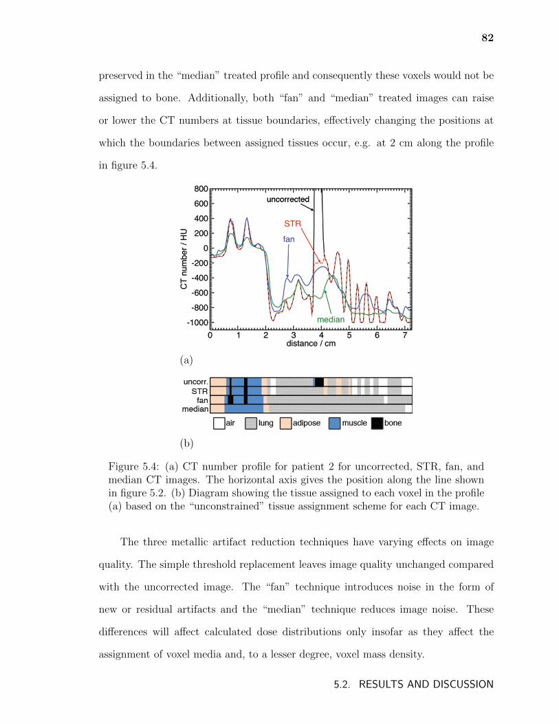
82
preserved in the “median” treated profile and consequently these voxels would not be
assigned to bone. Additionally, both “fan” and “median” treated images can raise
or lower the CT numbers at tissue boundaries, effectively changing the positions at
which the boundaries between assigned tissues occur, e.g. at 2 cm along the profile
in figure 5.4.
(a)
(b)
Figure 5.4: (a) CT number profile for patient 2 for uncorrected, STR, fan, andmedian CT images. The horizontal axis gives the position along the line shownin figure 5.2. (b) Diagram showing the tissue assigned to each voxel in the profile(a) based on the “unconstrained” tissue assignment scheme for each CT image.
The three metallic artifact reduction techniques have varying effects on image
quality. The simple threshold replacement leaves image quality unchanged compared
with the uncorrected image. The “fan” technique introduces noise in the form of
new or residual artifacts and the “median” technique reduces image noise. These
differences will affect calculated dose distributions only insofar as they affect the
assignment of voxel media and, to a lesser degree, voxel mass density.
5.2. RESULTS AND DISCUSSION
83
5.2.2 Tissue assignment schemes and dose
Tables 5.2-5.4 provide the minimum dose in the hottest 90% and the volume (D90) and
the percent volume that receives at least the prescription dose of 100 Gy (V100) for
PTV05 and PTV20 for patients 1, 2, and 5, respectively. Universally, the dose metrics
calculated using uncorrected, unconstrained phantoms are lower than for metallic ar-
tifact reduced and/or constrained phantoms due to higher CT numbers in the vicinity
of seeds resulting in voxels being assigned to dense bone (which considerably atten-
uates photons emitted from the seeds). Table 5.5 lists the percentage of voxels that
are assigned to bone in the immediate vicinity of seeds (which is defined as any voxel
within a 1 x 1 x 1 cm3 cube of a seed centre, corresponding to the volumes used for
“STR”) for a subset of phantom models. Visual inspection of CT images indicates
that a very small percentage of voxels in the seed ROIs of patients 1 and 2 are found
in the ribs but that no voxels in the seed ROIs of patient 5 are found in anatomical
bone. In agreement with the results of chapter 4, the mis-assignment of voxels to
bone causes the greatest difference in dose distributions between various models.
For all three patients, dose metrics increase dramatically when metallic arti-
fact correction methods are used. Dose metrics in unconstrained phantoms for pa-
tient 1 are approximately equal for phantoms that received “STR” and “fan+STR”,
but differ in phantoms that received “fan” and “median”. For patient 2, “STR”,
“fan+STR”, and “median” treated phantoms have dose metrics that differ from those
of “fan” treated phantoms for patient 2. In patient 5, D90 for PTV05 differs consider-
ably between phantoms derived using all four metallic artifact reduction techniques.
However, the considerably lower dose for “fan” and the relatively high percentage of
voxels assigned to bone for the “fan” unconstrained phantom for this patient (which
should have no bone in the vicinity of the seeds), suggests that the “fan” method did
5.2. RESULTS AND DISCUSSION
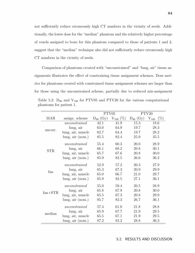
84
not sufficiently reduce erroneously high CT numbers in the vicinity of seeds. Addi-
tionally, the lower dose for the “median” phantom and the relatively higher percentage
of voxels assigned to bone for this phantom compared to those of patients 1 and 2,
suggest that the “median” technique also did not sufficiently reduce erroneously high
CT numbers in the vicinity of seeds.
Comparison of phantoms created with “unconstrained” and “lung, air” tissue as-
signments illustrates the effect of constraining tissue assignment schemes. Dose met-
rics for phantoms created with constrained tissue assignment schemes are larger than
for those using the unconstrained scheme, partially due to reduced mis-assignment
Table 5.2: D90 and V100 for PTV05 and PTV20 for the various computationalphantoms for patient 1.
PTV05 PTV20MAR assign. scheme D90 (Gy) V100 (%) D90 (Gy) V100 (%)
uncorr.
unconstrained 42.1 41.9 15.3 18.6lung, air 63.0 64.9 19.7 28.3
lung, air, muscle 62.7 64.4 19.7 28.2lung, air (nom.) 85.5 82.4 25.9 35.5
STR
unconstrained 55.4 60.3 20.0 28.9lung, air 66.1 68.2 20.8 30.1
lung, air, muscle 65.7 67.6 20.8 30.0lung, air (nom.) 85.9 82.5 26.6 36.2
fan
unconstrained 52.9 57.2 20.3 27.9lung, air 65.3 67.3 20.9 29.9
lung, air, muscle 65.0 66.7 21.0 29.7lung, air (nom.) 85.9 82.5 27.1 36.1
fan+STR
unconstrained 55.0 59.4 20.5 28.9lung, air 65.8 67.9 20.8 30.0
lung, air, muscle 65.5 67.3 20.8 29.9lung, air (nom.) 85.7 82.3 26.7 36.1
median
unconstrained 57.4 61.0 21.8 28.8lung, air 65.9 67.7 21.9 29.5
lung, air, muscle 65.5 67.1 21.9 29.5lung, air (nom.) 87.2 83.2 28.8 36.3
5.2. RESULTS AND DISCUSSION
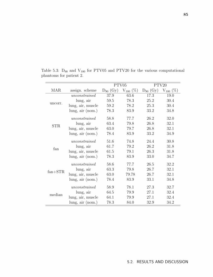
85
Table 5.3: D90 and V100 for PTV05 and PTV20 for the various computationalphantoms for patient 2.
PTV05 PTV20MAR assign. scheme D90 (Gy) V100 (%) D90 (Gy) V100 (%)
uncorr.
unconstrained 37.9 63.6 17.3 19.0lung, air 59.5 78.3 25.2 30.4
lung, air, muscle 59.2 78.2 25.3 30.4lung, air (nom.) 78.3 83.9 33.2 34.8
STR
unconstrained 58.8 77.7 26.2 32.0lung, air 63.4 79.8 26.8 32.1
lung, air, muscle 63.0 79.7 26.8 32.1lung, air (nom.) 78.4 83.9 33.2 34.9
fan
unconstrained 51.6 74.8 24.4 30.8lung, air 61.7 79.2 26.2 31.8
lung, air, muscle 61.5 79.1 26.3 31.8lung, air (nom.) 78.3 83.9 33.0 34.7
fan+STR
unconstrained 58.6 77.7 26.5 32.2lung, air 63.3 79.8 26.7 32.1
lung, air, muscle 63.0 79.78 26.7 32.1lung, air (nom.) 78.4 83.9 33.1 34.8
median
unconstrained 58.9 78.1 27.3 32.7lung, air 64.5 79.9 27.1 32.4
lung, air, muscle 64.1 79.9 27.1 32.4lung, air (nom.) 78.3 84.0 32.9 34.2
5.2. RESULTS AND DISCUSSION

86
Table 5.4: D90 and V100 for PTV05 and PTV20 for the various computationalphantoms for patient 5.
PTV05 PTV20MAR assign. scheme D90 (Gy) V100 (%) D90 (Gy) V100 (%)
uncorr.
unconstrained 68.1 77.4 18.6 18.4lung, air 92.6 87.8 24.5 25.7
lung, air, muscle 92.3 87.7 24.5 25.7lung, air (nom.) 102 90.6 28.4 29.5
STR
unconstrained 116 92.7 30.1 32.7lung, air 124 93.9 31.6 33.8
lung, air, muscle 124 93.9 31.6 33.8lung, air (nom.) 135 96.0 35.2 37.1
fan
unconstrained 94.7 88.8 26.3 28.6lung, air 109 91.8 28.4 30.5
lung, air, muscle 109 91.8 28.5 30.5lung, air (nom.) 118 94.0 31.9 33.7
fan+STR
unconstrained 114 92.3 30.3 32.3lung, air 123 93.7 31.3 33.3
lung, air, muscle 122 93.7 31.3 33.3lung, air (nom.) 134 95.9 35.0 36.9
median
unconstrained 110 91.6 30.2 31.3lung, air 123 93.7 30.4 32.0
lung, air, muscle 124 93.6 30.5 32.0lung, air (nom.) 139 96.3 34.6 35.8
5.2. RESULTS AND DISCUSSION
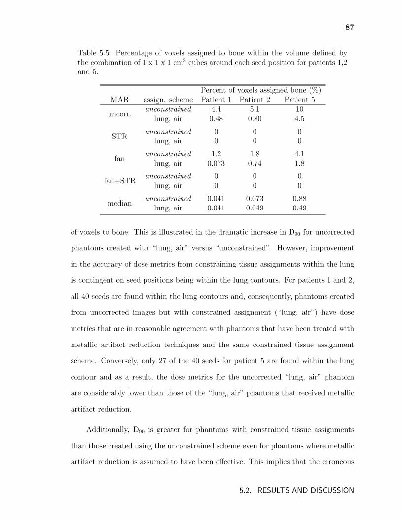
87
Table 5.5: Percentage of voxels assigned to bone within the volume defined bythe combination of 1 x 1 x 1 cm3 cubes around each seed position for patients 1,2and 5.
Percent of voxels assigned bone (%)MAR assign. scheme Patient 1 Patient 2 Patient 5
uncorr.unconstrained 4.4 5.1 10
lung, air 0.48 0.80 4.5
STRunconstrained 0 0 0
lung, air 0 0 0
fanunconstrained 1.2 1.8 4.1
lung, air 0.073 0.74 1.8
fan+STRunconstrained 0 0 0
lung, air 0 0 0
medianunconstrained 0.041 0.073 0.88
lung, air 0.041 0.049 0.49
of voxels to bone. This is illustrated in the dramatic increase in D90 for uncorrected
phantoms created with “lung, air” versus “unconstrained”. However, improvement
in the accuracy of dose metrics from constraining tissue assignments within the lung
is contingent on seed positions being within the lung contours. For patients 1 and 2,
all 40 seeds are found within the lung contours and, consequently, phantoms created
from uncorrected images but with constrained assignment (“lung, air”) have dose
metrics that are in reasonable agreement with phantoms that have been treated with
metallic artifact reduction techniques and the same constrained tissue assignment
scheme. Conversely, only 27 of the 40 seeds for patient 5 are found within the lung
contour and as a result, the dose metrics for the uncorrected “lung, air” phantom
are considerably lower than those of the “lung, air” phantoms that received metallic
artifact reduction.
Additionally, D90 is greater for phantoms with constrained tissue assignments
than those created using the unconstrained scheme even for phantoms where metallic
artifact reduction is assumed to have been effective. This implies that the erroneous
5.2. RESULTS AND DISCUSSION
88
assignment of adipose tissue in phantoms created using unconstrained tissue assign-
ments causes a small but notable decrease in dose metrics since the mass energy
absorption coefficient of adipose tissue is approximately 40% lower than that of lung
tissue.
The effects of metallic artifact reduction and constrained tissue assignment pre-
sented thus far are demonstrated in figure 5.5 which shows dose profiles along the
line shown in figure 5.2 (page 78) for phantoms derived from uncorrected and metal-
lic artifact corrected images using the “unconstrained” (fig. 5.5a) and “lung, air”
(fig. 5.5b) tissue assignment schemes. In figure 5.5a, the dose for the phantom that
received no artifact mitigation is considerably lower throughout due to the attenua-
tion of photons passing through erroneous bone tissue. The dose profiles for “STR”,
“fan”, and “median” treated phantoms are generally in reasonable agreement with a
few exceptions: near 1 cm, the phantom that received the “median” algorithm does
not model the rib (see figure 5.4b) resulting in a lower dose in these voxels; between 4
and 6 cm, voxels of air and adipose tissue in the phantom that received “STR” absorb
less dose than the lung voxels in the phantoms that received “fan” or “median”; and
at approximately 0.6 cm where more voxels are assigned bone in for the “fan” treated
phantom and consequently the dose is higher in those voxels. In figure 5.5b, voxels
beyond 2 cm from the start of the profile are inside the lung contour and are only
assigned to lung or air for each phantom. Consequently, the dose profiles are all in
reasonable agreement with only small differences in dose due to differences in voxel
densities.
Phantoms created with constrained tissue assignments that allow lung, air, and
muscle to be assigned within the lung contour produce dose metrics that are in close
agreement with phantoms that have only lung and air within lung contours (tables
5.2-5.4). While lung and muscle tissues differ in atomic composition, their mass at-
5.2. RESULTS AND DISCUSSION
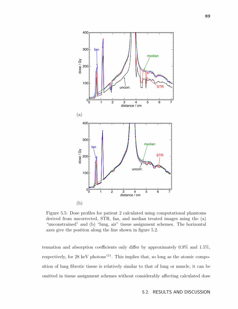
89
0 1 2 3 4 5 6 7distance / cm
0
100
200
300
400
dose
/ G
y
uncorr. STR
medianfan
(a)
0 1 2 3 4 5 6 7distance / cm
0
100
200
300
400
dose
/ G
y
uncorr.
fanmedian
STR
(b)
Figure 5.5: Dose profiles for patient 2 calculated using computational phantomsderived from uncorrected, STR, fan, and median treated images using the (a)“unconstrained” and (b) “lung, air” tissue assignment schemes. The horizontalaxes give the position along the line shown in figure 5.2.
tenuation and absorption coefficients only differ by approximately 0.9% and 1.5%,
respectively, for 28 keV photons111. This implies that, so long as the atomic compo-
sition of lung fibrotic tissue is relatively similar to that of lung or muscle, it can be
omitted in tissue assignment schemes without considerably affecting calculated dose
5.2. RESULTS AND DISCUSSION
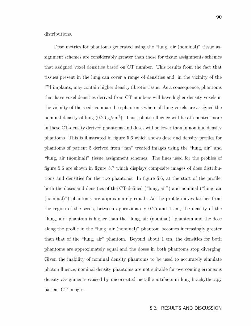
90
distributions.
Dose metrics for phantoms generated using the “lung, air (nominal)” tissue as-
signment schemes are considerably greater than those for tissue assignments schemes
that assigned voxel densities based on CT number. This results from the fact that
tissues present in the lung can cover a range of densities and, in the vicinity of the
125I implants, may contain higher density fibrotic tissue. As a consequence, phantoms
that have voxel densities derived from CT numbers will have higher density voxels in
the vicinity of the seeds compared to phantoms where all lung voxels are assigned the
nominal density of lung (0.26 g/cm3). Thus, photon fluence will be attenuated more
in these CT-density derived phantoms and doses will be lower than in nominal density
phantoms. This is illustrated in figure 5.6 which shows dose and density profiles for
phantoms of patient 5 derived from “fan” treated images using the “lung, air” and
“lung, air (nominal)” tissue assignment schemes. The lines used for the profiles of
figure 5.6 are shown in figure 5.7 which displays composite images of dose distribu-
tions and densities for the two phantoms. In figure 5.6, at the start of the profile,
both the doses and densities of the CT-defined (“lung, air”) and nominal (“lung, air
(nominal)”) phantoms are approximately equal. As the profile moves farther from
the region of the seeds, between approximately 0.25 and 1 cm, the density of the
“lung, air” phantom is higher than the “lung, air (nominal)” phantom and the dose
along the profile in the “lung, air (nominal)” phantom becomes increasingly greater
than that of the “lung, air” phantom. Beyond about 1 cm, the densities for both
phantoms are approximately equal and the doses in both phantoms stop diverging.
Given the inability of nominal density phantoms to be used to accurately simulate
photon fluence, nominal density phantoms are not suitable for overcoming erroneous
density assignments caused by uncorrected metallic artifacts in lung brachytherapy
patient CT images.
5.2. RESULTS AND DISCUSSION
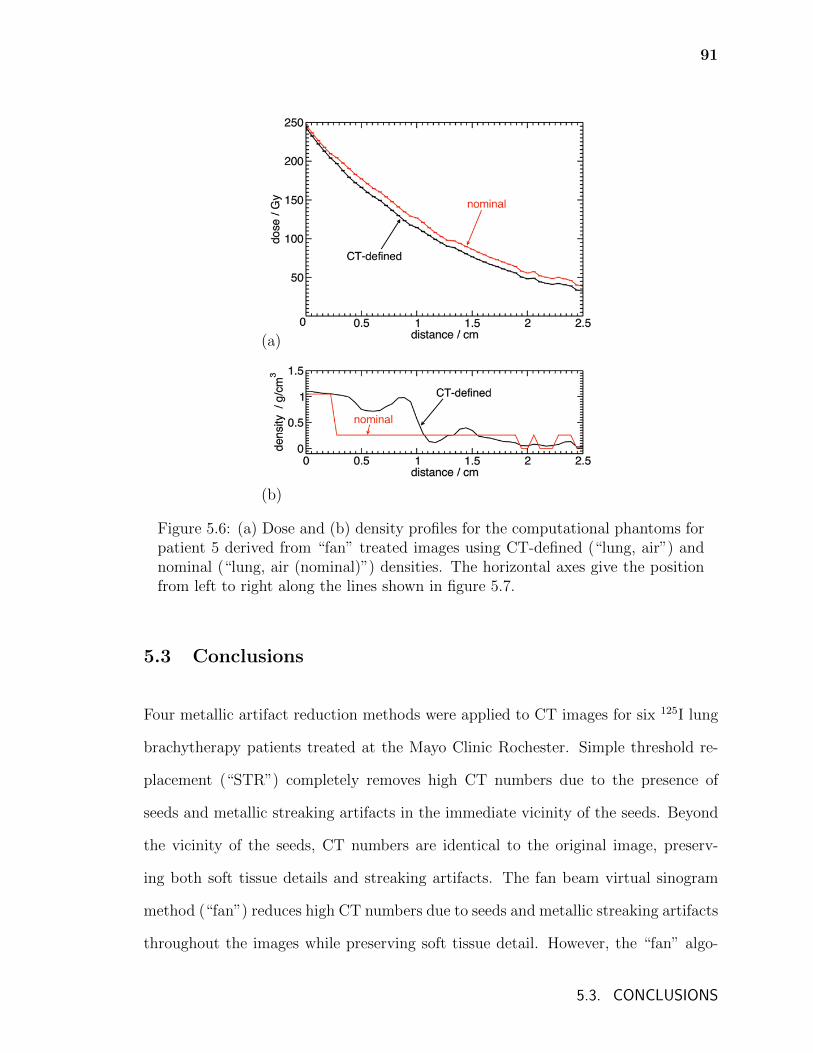
91
(a)
(b)
Figure 5.6: (a) Dose and (b) density profiles for the computational phantoms forpatient 5 derived from “fan” treated images using CT-defined (“lung, air”) andnominal (“lung, air (nominal)”) densities. The horizontal axes give the positionfrom left to right along the lines shown in figure 5.7.
5.3 Conclusions
Four metallic artifact reduction methods were applied to CT images for six 125I lung
brachytherapy patients treated at the Mayo Clinic Rochester. Simple threshold re-
placement (“STR”) completely removes high CT numbers due to the presence of
seeds and metallic streaking artifacts in the immediate vicinity of the seeds. Beyond
the vicinity of the seeds, CT numbers are identical to the original image, preserv-
ing both soft tissue details and streaking artifacts. The fan beam virtual sinogram
method (“fan”) reduces high CT numbers due to seeds and metallic streaking artifacts
throughout the images while preserving soft tissue detail. However, the “fan” algo-
5.3. CONCLUSIONS
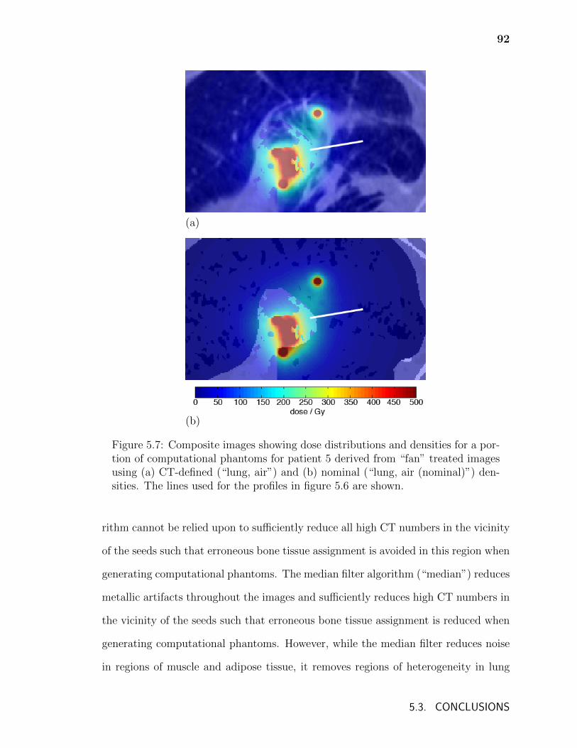
92
(a)
(b)
Figure 5.7: Composite images showing dose distributions and densities for a por-tion of computational phantoms for patient 5 derived from “fan” treated imagesusing (a) CT-defined (“lung, air”) and (b) nominal (“lung, air (nominal)”) den-sities. The lines used for the profiles in figure 5.6 are shown.
rithm cannot be relied upon to sufficiently reduce all high CT numbers in the vicinity
of the seeds such that erroneous bone tissue assignment is avoided in this region when
generating computational phantoms. The median filter algorithm (“median”) reduces
metallic artifacts throughout the images and sufficiently reduces high CT numbers in
the vicinity of the seeds such that erroneous bone tissue assignment is reduced when
generating computational phantoms. However, while the median filter reduces noise
in regions of muscle and adipose tissue, it removes regions of heterogeneity in lung
5.3. CONCLUSIONS
93
tissue and can reduce the CT numbers for voxels representing bone tissue such that
tissue mis-assignment occurs. Median filter techniques might be appropriate in treat-
ment sites such as the prostate where seeds are located in regions that have less tissue
heterogeneity. A combination of a fan beam virtual sinogram treatment followed by
a simple threshold replacement (“fan+STR”) sufficiently reduces high CT numbers
due to seeds such that bone mis-assignment is avoided, while simultaneously reduc-
ing streaking artifacts and preserving tissue heterogeneities beyond the immediate
vicinity of the seeds.
Full Monte Carlo calculations were performed for three of the six Mayo Clinic
patients using computational phantoms generated by applying various tissue assign-
ment schemes to the CT image sets. Constrained tissue assignment within lung
contours reduces misassignment of voxels to bone in lung contours and so can be
used to ameliorate the effects of suboptimal metallic artifact reduction. However,
this improvement is contingent on the 125I seeds being found within the lung contour,
which may not always be the case. Additionally, lung-constrained tissue assignment
impedes the misassignment of voxels to adipose tissue, avoiding inaccuracies in dose
distributions and dose metrics caused by the considerably lower mass attenuation and
energy absorption coefficients of adipose tissue compared to lung tissue.111
A tissue assignment scheme that allows the assignment of muscle tissue within
lung contours produces phantoms with resulting dose distributions that are approxi-
mately equal to those produced by a tissue assignment scheme that only allows lung
and air to be assigned. This implies that, as long as the unknown atomic composition
(and resulting mass attenuation and energy absorption coefficients) of lung fibrotic
tissue does not differ considerably from that of lung or muscle, the presence of fibrotic
tissue can be omitted from tissue assignment schemes without reducing the accuracy
of calculated dose distributions.
5.3. CONCLUSIONS
94
Computational phantoms with voxel densities assigned as the nominal density
of the local voxel medium are not suitable for generating accurate dose distributions
for lung brachytherapy patients as the nominal density of lung (0.26 g/cm3) does not
accurately represent the varied density of the lung tissue in the vicinity of the seeds.
The model that produced the most accurate Monte Carlo calculated dose dis-
tributions for lung brachytherapy patients (of the phantom models discussed) is a
phantom generated by applying a tissue assignment scheme where only lung and air
are assigned within lung contours to CT images that have been treated with a fan
beam virtual sinogram algorithm followed by a simple threshold replacement algo-
rithm. Since misassignment of tissues can considerably affect doses even when metallic
artifacts are reduced, following the recommendation by the AAPM Task Group re-
port 186 (Ref. 29) of using organ contours to guide tissue assignment will produce
more realistic computational phantoms and consequently more accurate model-based
dose calculations for brachytherapy in general.
5.3. CONCLUSIONS
Chapter 6
A Monte Carlo investigation of
lung brachytherapy treatment planning
This chapter investigates avenues for an improved paradigm for lung brachytherapy
treatment planning, drawing on the knowledge of media heterogeneity effects from
chapters 4 and 5. Significant approximations are used in the standard practices for
dosimetry and treatment planning for permanent implant lung brachytherapy. The
area at risk of recurrence is determined intra-operatively and treatment planning
only involves the use of a seed activity nomogram or look-up table to determine
the seed spacing for the grid pattern mesh implant9,15. Nomograms are typically
calculated using the TG-43 formalism25–27, i.e. doses are calculated assuming sources
in a homogeneous water environment, with no interseed effects, and the point source
approximation of the TG-43 formalism is often used.
In addition to 125I seeds, 131Cs seeds have also been used for lung brachyther-
apy and TG-43 calculated dose distributions have been compared between the two
radionuclides21. However, having different emitted photon energy spectra, the devia-
tions between TG-43 and model-based (including non-water media) calculated doses
will differ between 125I and 131Cs treatments due to differences in mass attenuation
and energy absorption coefficients.
95
96
Given the significant deviations between TG-43 and MC dose distributions found
in chapter 4, it is likely that there are significant differences between prescribed and
delivered doses. Additionally, implantation of the planar mesh grid in patients leads
to deformation of the plane of sources used for treatment planning and for prescription
dose calculation. This deformation varies with implant site and, in conjunction with
differences in the composition of surrounding tissues at different implant sites, will
likely lead to large discrepancies between planned and delivered doses.
In this chapter, the accuracy of lung brachytherapy prescription doses calcu-
lated using TG-43 derived nomograms is investigated. Nomogram doses for planar
source configurations are recalculated with BrachyDose using a variety of tissue mod-
els and these doses are compared to TG-43 calculated prescription doses. To in-
vestigate the changes in dose distributions between those of nomogram models and
deformed implants in patients, a method of generating patient specific virtual im-
plants is developed. Virtual implants are modelled for several example resection sites
and Monte Carlo calculated dose distributions in a CT-derived patient phantom for
these implants are compared to nomogram model dose distributions. Calculations
are performed using both 125I and 131Cs seeds.
6.1 Methods
This chapter is comprised of two parts, described in the following sections: Section
6.1.1 investigates the effects of non-water media and interseed attenuation on pre-
scription dose, assuming the planar seed configuration currently used for treatment
planning. Section 6.1.2 considers deformation of the planar seed configuration, re-
flecting more realistic seed configurations encountered in patient treatments.
Calculations are for 125I GE Healthcare/Oncura (Arlington Heights IL USA)
6.1. METHODS
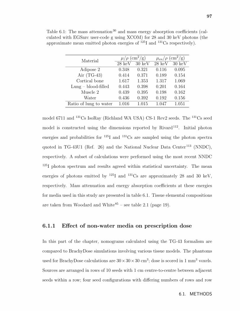
97
Table 6.1: The mass attenuation30 and mass energy absorption coefficients (cal-culated with EGSnrc user-code g using XCOM) for 28 and 30 keV photons (theapproximate mean emitted photon energies of 125I and 131Cs respectively).
Materialµ/ρ (cm2/g) µen/ρ (cm2/g)
28 keV 30 keV 28 keV 30 keVAdipose 2 0.348 0.321 0.116 0.095
Air (TG-43) 0.414 0.371 0.189 0.154Cortical bone 1.617 1.353 1.317 1.069
Lung – blood-filled 0.443 0.398 0.201 0.164Muscle 2 0.439 0.395 0.198 0.162
Water 0.436 0.392 0.192 0.156Ratio of lung to water 1.016 1.015 1.047 1.051
model 6711 and 131Cs IsoRay (Richland WA USA) CS-1 Rev2 seeds. The 131Cs seed
model is constructed using the dimensions reported by Rivard112. Initial photon
energies and probabilities for 125I and 131Cs are sampled using the photon spectra
quoted in TG-43U1 (Ref. 26) and the National Nuclear Data Center113 (NNDC),
respectively. A subset of calculations were performed using the most recent NNDC
125I photon spectrum and results agreed within statistical uncertainty. The mean
energies of photons emitted by 125I and 131Cs are approximately 28 and 30 keV,
respectively. Mass attenuation and energy absorption coefficients at these energies
for media used in this study are presented in table 6.1. Tissue elemental compositions
are taken from Woodard and White85 – see table 2.1 (page 19).
6.1.1 Effect of non-water media on prescription dose
In this part of the chapter, nomograms calculated using the TG-43 formalism are
compared to BrachyDose simulations involving various tissue models. The phantoms
used for BrachyDose calculations are 30×30×30 cm3; dose is scored in 1 mm3 voxels.
Sources are arranged in rows of 10 seeds with 1 cm centre-to-centre between adjacent
seeds within a row; four seed configurations with differing numbers of rows and row
6.1. METHODS
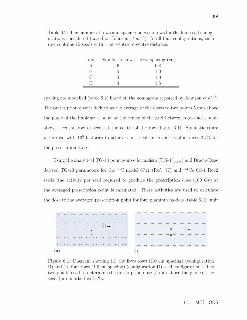
98
Table 6.2: The number of rows and spacing between rows for the four seed config-urations considered (based on Johnson et al.15). In all four configurations, eachrow contains 10 seeds with 1 cm centre-to-centre distance.
Label Number of rows Row spacing (cm)A 6 0.8B 5 1.0C 4 1.3D 4 1.5
spacing are modelled (table 6.2) based on the nomogram reported by Johnson et al.15.
The prescription dose is defined as the average of the doses to two points 5 mm above
the plane of the implant: a point at the centre of the grid between rows and a point
above a central row of seeds at the centre of the row (figure 6.1). Simulations are
performed with 109 histories to achieve statistical uncertainties of at most 0.4% for
the prescription dose.
Using the analytical TG-43 point source formalism (TG-43point) and BrachyDose
derived TG-43 parameters for the 125I model 6711 (Ref. 77) and 131Cs CS-1 Rev2
seeds, the activity per seed required to produce the prescription dose (100 Gy) at
the averaged prescription point is calculated. These activities are used to calculate
the dose to the averaged prescription point for four phantom models (table 6.3): unit
(a) (b)
Figure 6.1: Diagram showing (a) the fives rows (1.0 cm spacing) (configurationB) and (b) four rows (1.5 cm spacing) (configuration D) seed configurations. Thetwo points used to determine the prescription dose (5 mm above the plane of theseeds) are marked with Xs.
6.1. METHODS
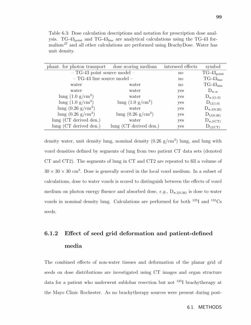
99
Table 6.3: Dose calculation descriptions and notation for prescription dose anal-ysis. TG-43point and TG-43line are analytical calculations using the TG-43 for-malism27 and all other calculations are performed using BrachyDose. Water hasunit density.
phant. for photon transport dose scoring medium interseed effects symbol– TG-43 point source model – no TG-43point
– TG-43 line source model – no TG-43line
water water no TG-43sim
water water yes Dw,w
lung (1.0 g/cm3) water yes Dw,l(1.0)
lung (1.0 g/cm3) lung (1.0 g/cm3) yes Dl,l(1.0)
lung (0.26 g/cm3) water yes Dw,l(0.26)
lung (0.26 g/cm3) lung (0.26 g/cm3) yes Dl,l(0.26)
lung (CT derived den.) water yes Dw,l(CT)
lung (CT derived den.) lung (CT derived den.) yes Dl,l(CT)
density water, unit density lung, nominal density (0.26 g/cm3) lung, and lung with
voxel densities defined by segments of lung from two patient CT data sets (denoted
CT and CT2). The segments of lung in CT and CT2 are repeated to fill a volume of
30 × 30 × 30 cm3. Dose is generally scored in the local voxel medium. In a subset of
calculations, dose to water voxels is scored to distinguish between the effects of voxel
medium on photon energy fluence and absorbed dose, e.g., Dw,l(0.26) is dose to water
voxels in nominal density lung. Calculations are performed for both 125I and 131Cs
seeds.
6.1.2 Effect of seed grid deformation and patient-defined
media
The combined effects of non-water tissues and deformation of the planar grid of
seeds on dose distributions are investigated using CT images and organ structure
data for a patient who underwent sublobar resection but not 125I brachytherapy at
the Mayo Clinic Rochester. As no brachytherapy sources were present during post-
6.1. METHODS
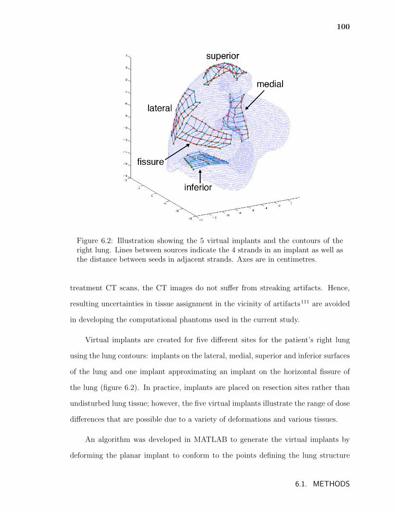
100
Figure 6.2: Illustration showing the 5 virtual implants and the contours of theright lung. Lines between sources indicate the 4 strands in an implant as well asthe distance between seeds in adjacent strands. Axes are in centimetres.
treatment CT scans, the CT images do not suffer from streaking artifacts. Hence,
resulting uncertainties in tissue assignment in the vicinity of artifacts111 are avoided
in developing the computational phantoms used in the current study.
Virtual implants are created for five different sites for the patient’s right lung
using the lung contours: implants on the lateral, medial, superior and inferior surfaces
of the lung and one implant approximating an implant on the horizontal fissure of
the lung (figure 6.2). In practice, implants are placed on resection sites rather than
undisturbed lung tissue; however, the five virtual implants illustrate the range of dose
differences that are possible due to a variety of deformations and various tissues.
An algorithm was developed in MATLAB to generate the virtual implants by
deforming the planar implant to conform to the points defining the lung structure
6.1. METHODS
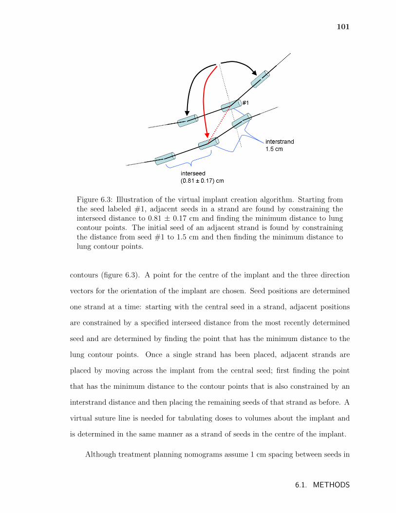
101
Figure 6.3: Illustration of the virtual implant creation algorithm. Starting fromthe seed labeled #1, adjacent seeds in a strand are found by constraining theinterseed distance to 0.81 ± 0.17 cm and finding the minimum distance to lungcontour points. The initial seed of an adjacent strand is found by constrainingthe distance from seed #1 to 1.5 cm and then finding the minimum distance tolung contour points.
contours (figure 6.3). A point for the centre of the implant and the three direction
vectors for the orientation of the implant are chosen. Seed positions are determined
one strand at a time: starting with the central seed in a strand, adjacent positions
are constrained by a specified interseed distance from the most recently determined
seed and are determined by finding the point that has the minimum distance to the
lung contour points. Once a single strand has been placed, adjacent strands are
placed by moving across the implant from the central seed; first finding the point
that has the minimum distance to the contour points that is also constrained by an
interstrand distance and then placing the remaining seeds of that strand as before. A
virtual suture line is needed for tabulating doses to volumes about the implant and
is determined in the same manner as a strand of seeds in the centre of the implant.
Although treatment planning nomograms assume 1 cm spacing between seeds in
6.1. METHODS
102
a strand, interseed distance varies following implantation. Interseed distances of four
Mayo Clinic patients treated with 125I lung mesh brachytherapy were calculated and
are found to vary randomly with a mean value of 0.81 cm and standard deviation
of 0.17 cm. This distribution is used to randomly assign interseed distances when
generating the virtual implants. An interstrand distance of 1.5 cm corresponding to
configuration D in table 6.2 is used for the central seeds of each strand where distances
between strands is constrained.
A phantom is created using CT data and a tissue assignment scheme that in-
cludes adipose, air, cortical bone, lung, and muscle, corresponding to the “simple”
assignment scheme of chapter 4. This phantom is cropped to span approximately 30
cm in each direction centred on the right lung and, using original voxels sizes, has
239 voxels with a width of 0.125 cm in the anterior-posterior and lateral directions
and 119 voxels with a width of 0.25 cm in the superior-inferior direction.
Monte Carlo calculated dose distributions for brachytherapy are sensitive to the
conversion of CT image pixel values to atomic composition48,108. By varying atomic
composition, Landry et al.42 found up to 4% and 10% differences in the the minimum
dose received by 90% of planning treatment volumes (D90) for prostate and breast
brachytherapy treatments, respectively. Chapters 4 and 5 presented significant dif-
ferences in dose metrics for lung brachytherapy patients based on the use of different
tissue assignment schemes. Consequently, the dose distributions presented in section
6.2.2 are dependent on the tissue assignment scheme chosen and they will be affected
by errors in tissue assignment and so should be considered examples of the effects
discussed.
Dose to water voxels in a water phantom with no interseed attenuation (TG-
43sim), dose to water voxels in a CT-derived tissue phantom (Dw,m(CT)), and dose to
the local voxel medium in a CT-derived tissue phantom (Dm,m(CT)) are calculated.
6.1. METHODS
103
For comparison, TG-43sim doses and Dl,l(0.26) for the planar nomogram configuration
D from table 6.2 (page 98) and section 6.1.1 (denoted as “planar D”) as well as for a
modified configuration where the in-row interseed spacing is 0.81 cm (denoted “planar
(0.81) D”) are calculated. Doses from 125I and 131Cs seeds are calculated and, in all
cases, calculations are performed using the activity that would produce a dose of 100
Gy to the averaged prescription point of planar configuration D using TG-43sim. For
each of the different implant configurations, dose volume histograms are calculated
for volumes consisting of voxels with centres that are within 5 mm and 20 mm of each
implant’s suture line (referred to as PTV05 and PTV20, respectively). Simulations
are performed with 4 × 10⁹ histories taking approximately 23 CPU hours on a single
3.0 GHz Woodcrest core to achieve a maximum statistical uncertainty of less than
0.4% in PTV20 volumes.
6.2 Results and discussion
6.2.1 Effect of non-water media on prescription dose
Figure 6.4 shows the dose to the averaged prescription point calculated for seed con-
figuration A (6 rows with 0.8 cm spacing) for each of the phantom models divided by
the TG-43point calculated dose and using the same source activity; results are shown
for both 125I and 131Cs seeds. This dose ratio shows the deviation in the prescription
dose for each dose calculation model compared to the TG-43point derived nomogram.
Focusing on the results in figure 6.4 for 125I, the TG-43line calculation is 2%
smaller than TG-43point due largely to differences between the anisotropy function
and anisotropy factor. TG-43sim is smaller than TG-43point by less than one percent;
this difference is 2% when interseed attenuation is included (Dw,w). For Dw,l(1.0), the
6.2. RESULTS AND DISCUSSION
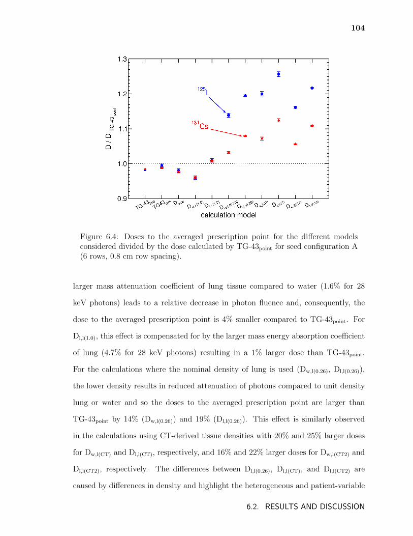
104
Figure 6.4: Doses to the averaged prescription point for the different modelsconsidered divided by the dose calculated by TG-43point for seed configuration A(6 rows, 0.8 cm row spacing).
larger mass attenuation coefficient of lung tissue compared to water (1.6% for 28
keV photons) leads to a relative decrease in photon fluence and, consequently, the
dose to the averaged prescription point is 4% smaller compared to TG-43point. For
Dl,l(1.0), this effect is compensated for by the larger mass energy absorption coefficient
of lung (4.7% for 28 keV photons) resulting in a 1% larger dose than TG-43point.
For the calculations where the nominal density of lung is used (Dw,l(0.26), Dl,l(0.26)),
the lower density results in reduced attenuation of photons compared to unit density
lung or water and so the doses to the averaged prescription point are larger than
TG-43point by 14% (Dw,l(0.26)) and 19% (Dl,l(0.26)). This effect is similarly observed
in the calculations using CT-derived tissue densities with 20% and 25% larger doses
for Dw,l(CT) and Dl,l(CT), respectively, and 16% and 22% larger doses for Dw,l(CT2) and
Dl,l(CT2), respectively. The differences between Dl,l(0.26), Dl,l(CT), and Dl,l(CT2) are
caused by differences in density and highlight the heterogeneous and patient-variable
6.2. RESULTS AND DISCUSSION
105
nature of the lung.
The trends of dose to the averaged prescription point with varying tissue model
are less pronounced for 131Cs than for 125I. While the mass attenuation coefficient
ratio of lung to water is very similar for the mean emitted photon energies of 125I and
131Cs, the mass attenuation coefficient of lung at the mean emitted photon energy
of 131Cs is approximately 10% smaller than that for 125I; thus, the photon fluence
emitted from the 131Cs sources is attenuated less than that from 125I. Since the average
distance from a seed to the averaged prescription points remains the same, changes
in photon fluence between water and nominal density lung or CT-density lung will be
less pronounced for 131Cs. Additionally, since the mass energy absorption coefficient
ratio of lung to water is similar for 125I and 131Cs spectra, differences between dose to
lung voxels and dose to water voxels remain similar between 125I and 131Cs implants.
Figure 6.5 shows the isodose contours with 125I seeds comparing a TG-43sim cal-
culation with an activity chosen to produce 100 Gy at the averaged prescription point
and the same activity in a Dl,l(0.26) calculation for seed configuration C. The ∼20%
difference near the averaged prescription point (fig. 6.4) is seen with the 100 Gy iso-
dose line for TG-43sim nearly overlapping the 125 Gy line for Dl,l(0.26). The relative
difference in dose between the two calculations increases as the distance from the im-
plant increases with the 10 Gy isodose line for TG-43sim nearly overlapping the 25 Gy
line for Dl,l(0.26). Thus, beyond generally underestimating the dose to the averaged
prescription point, TG-43point also likely underestimates total lung doses and doses
to organs at risk.
The differences in dose to the averaged prescription point seen in figure 6.4 can be
generalized to all four seed configurations. However, the magnitude of the differences
between TG-43point and doses to nominal density lung and CT-density lung depend on
seed configuration. The dose to the averaged prescription point for Dl,l(0.26) divided by
6.2. RESULTS AND DISCUSSION
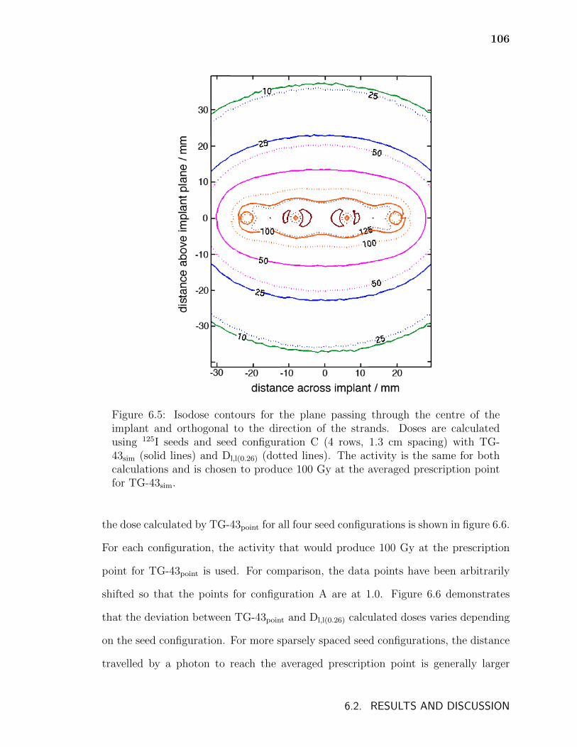
106
Figure 6.5: Isodose contours for the plane passing through the centre of theimplant and orthogonal to the direction of the strands. Doses are calculatedusing 125I seeds and seed configuration C (4 rows, 1.3 cm spacing) with TG-43sim (solid lines) and Dl,l(0.26) (dotted lines). The activity is the same for bothcalculations and is chosen to produce 100 Gy at the averaged prescription pointfor TG-43sim.
the dose calculated by TG-43point for all four seed configurations is shown in figure 6.6.
For each configuration, the activity that would produce 100 Gy at the prescription
point for TG-43point is used. For comparison, the data points have been arbitrarily
shifted so that the points for configuration A are at 1.0. Figure 6.6 demonstrates
that the deviation between TG-43point and Dl,l(0.26) calculated doses varies depending
on the seed configuration. For more sparsely spaced seed configurations, the distance
travelled by a photon to reach the averaged prescription point is generally larger
6.2. RESULTS AND DISCUSSION
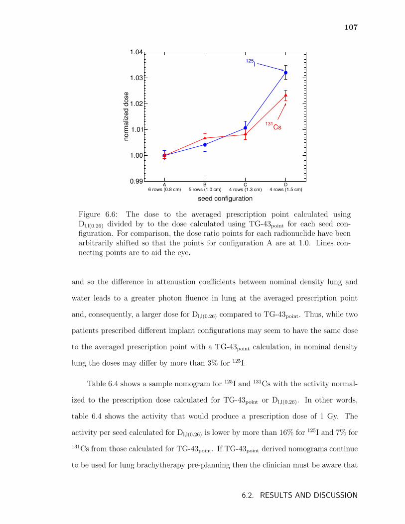
107
A6 rows (0.8 cm)
B5 rows (1.0 cm)
C4 rows (1.3 cm)
D4 rows (1.5 cm)
seed configuration
0.99
1.00
1.01
1.02
1.03
1.04
norm
aliz
ed d
ose
125I
131Cs
Figure 6.6: The dose to the averaged prescription point calculated usingDl,l(0.26) divided by to the dose calculated using TG-43point for each seed con-figuration. For comparison, the dose ratio points for each radionuclide have beenarbitrarily shifted so that the points for configuration A are at 1.0. Lines con-necting points are to aid the eye.
and so the difference in attenuation coefficients between nominal density lung and
water leads to a greater photon fluence in lung at the averaged prescription point
and, consequently, a larger dose for Dl,l(0.26) compared to TG-43point. Thus, while two
patients prescribed different implant configurations may seem to have the same dose
to the averaged prescription point with a TG-43point calculation, in nominal density
lung the doses may differ by more than 3% for 125I.
Table 6.4 shows a sample nomogram for 125I and 131Cs with the activity normal-
ized to the prescription dose calculated for TG-43point or Dl,l(0.26). In other words,
table 6.4 shows the activity that would produce a prescription dose of 1 Gy. The
activity per seed calculated for Dl,l(0.26) is lower by more than 16% for 125I and 7% for
131Cs from those calculated for TG-43point. If TG-43point derived nomograms continue
to be used for lung brachytherapy pre-planning then the clinician must be aware that
6.2. RESULTS AND DISCUSSION
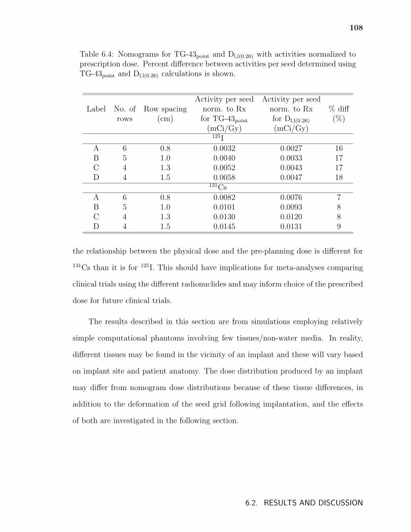
108
Table 6.4: Nomograms for TG-43point and Dl,l(0.26) with activities normalized toprescription dose. Percent difference between activities per seed determined usingTG-43point and Dl,l(0.26) calculations is shown.
Activity per seed Activity per seedLabel No. of Row spacing norm. to Rx norm. to Rx % diff
rows (cm) for TG-43point for Dl,l(0.26) (%)(mCi/Gy) (mCi/Gy)
125IA 6 0.8 0.0032 0.0027 16B 5 1.0 0.0040 0.0033 17C 4 1.3 0.0052 0.0043 17D 4 1.5 0.0058 0.0047 18
131CsA 6 0.8 0.0082 0.0076 7B 5 1.0 0.0101 0.0093 8C 4 1.3 0.0130 0.0120 8D 4 1.5 0.0145 0.0131 9
the relationship between the physical dose and the pre-planning dose is different for
131Cs than it is for 125I. This should have implications for meta-analyses comparing
clinical trials using the different radionuclides and may inform choice of the prescribed
dose for future clinical trials.
The results described in this section are from simulations employing relatively
simple computational phantoms involving few tissues/non-water media. In reality,
different tissues may be found in the vicinity of an implant and these will vary based
on implant site and patient anatomy. The dose distribution produced by an implant
may differ from nomogram dose distributions because of these tissue differences, in
addition to the deformation of the seed grid following implantation, and the effects
of both are investigated in the following section.
6.2. RESULTS AND DISCUSSION
109
0 50 100 150 200 250dose / Gy
0
20
40
60
80
100
pe
rce
nt
of
PT
V0
5 /
%
planar D
planar (0.81) D
lateral
medial
fissure
inferior
superior
Figure 6.7: TG-43sim dose volume histograms for PTV05 for the five virtual im-plants (fissure, inferior, lateral, medial, and superior) and for the planar nomo-gram configuration D with interseed spacings 1.0 cm (planar D) and 0.81 cm(planar (0.81) D) 125I seeds. Dose of 100 Gy is marked.
6.2.2 Effect of seed grid deformation and patient-defined
media
Figure 6.7 presents dose volume histograms for PTV05 calculated for TG-43sim for the
virtual implants compared to the planar nomogram configuration D and illustrates
how delivered dose can change due to implant deformation. The dose distribution
varies significantly based on the shape of the implant following deformation. The
doses for the superior implant, which is the most curved of the virtual implants,
deviate the most from those calculated using the planar configuration. In general,
differences in DVHs can be understood by considering the severity of the implant
deformation; implants that are quite deformed with smaller averaged distances from
seeds to the suture line have larger doses.
Differences between DVHs calculated with the planar D seed configuration with
6.2. RESULTS AND DISCUSSION
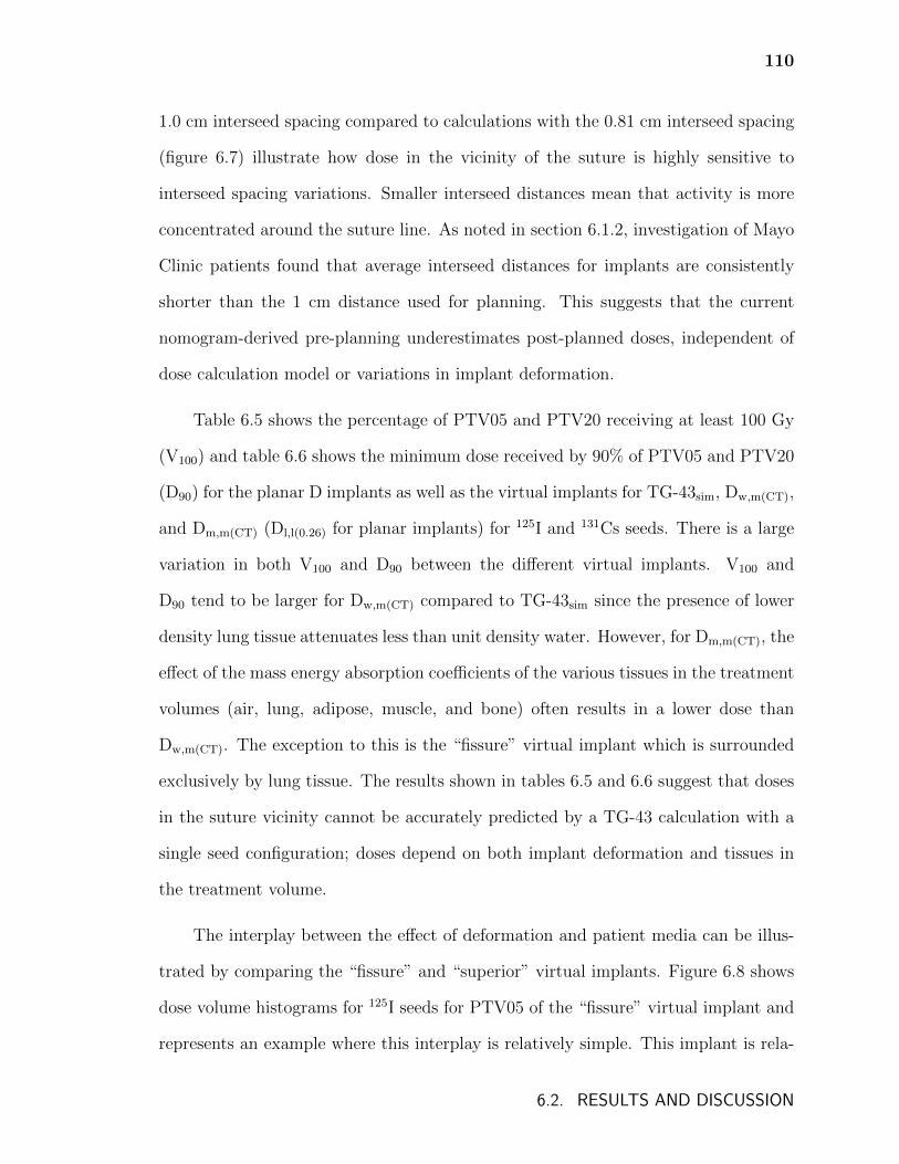
110
1.0 cm interseed spacing compared to calculations with the 0.81 cm interseed spacing
(figure 6.7) illustrate how dose in the vicinity of the suture is highly sensitive to
interseed spacing variations. Smaller interseed distances mean that activity is more
concentrated around the suture line. As noted in section 6.1.2, investigation of Mayo
Clinic patients found that average interseed distances for implants are consistently
shorter than the 1 cm distance used for planning. This suggests that the current
nomogram-derived pre-planning underestimates post-planned doses, independent of
dose calculation model or variations in implant deformation.
Table 6.5 shows the percentage of PTV05 and PTV20 receiving at least 100 Gy
(V100) and table 6.6 shows the minimum dose received by 90% of PTV05 and PTV20
(D90) for the planar D implants as well as the virtual implants for TG-43sim, Dw,m(CT),
and Dm,m(CT) (Dl,l(0.26) for planar implants) for 125I and 131Cs seeds. There is a large
variation in both V100 and D90 between the different virtual implants. V100 and
D90 tend to be larger for Dw,m(CT) compared to TG-43sim since the presence of lower
density lung tissue attenuates less than unit density water. However, for Dm,m(CT), the
effect of the mass energy absorption coefficients of the various tissues in the treatment
volumes (air, lung, adipose, muscle, and bone) often results in a lower dose than
Dw,m(CT). The exception to this is the “fissure” virtual implant which is surrounded
exclusively by lung tissue. The results shown in tables 6.5 and 6.6 suggest that doses
in the suture vicinity cannot be accurately predicted by a TG-43 calculation with a
single seed configuration; doses depend on both implant deformation and tissues in
the treatment volume.
The interplay between the effect of deformation and patient media can be illus-
trated by comparing the “fissure” and “superior” virtual implants. Figure 6.8 shows
dose volume histograms for 125I seeds for PTV05 of the “fissure” virtual implant and
represents an example where this interplay is relatively simple. This implant is rela-
6.2. RESULTS AND DISCUSSION
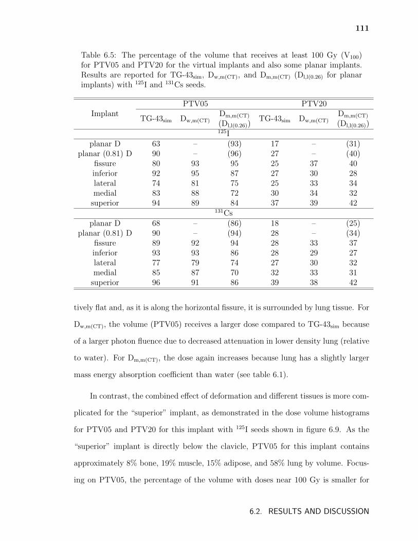
111
Table 6.5: The percentage of the volume that receives at least 100 Gy (V100)for PTV05 and PTV20 for the virtual implants and also some planar implants.Results are reported for TG-43sim, Dw,m(CT), and Dm,m(CT) (Dl,l(0.26) for planarimplants) with 125I and 131Cs seeds.
ImplantPTV05 PTV20
TG-43sim Dw,m(CT)Dm,m(CT) TG-43sim Dw,m(CT)
Dm,m(CT)
(Dl,l(0.26)) (Dl,l(0.26))125I
planar D 63 – (93) 17 – (31)planar (0.81) D 90 – (96) 27 – (40)
fissure 80 93 95 25 37 40inferior 92 95 87 27 30 28lateral 74 81 75 25 33 34medial 83 88 72 30 34 32
superior 94 89 84 37 39 42131Cs
planar D 68 – (86) 18 – (25)planar (0.81) D 90 – (94) 28 – (34)
fissure 89 92 94 28 33 37inferior 93 93 86 28 29 27lateral 77 79 74 27 30 32medial 85 87 70 32 33 31
superior 96 91 86 39 38 42
tively flat and, as it is along the horizontal fissure, it is surrounded by lung tissue. For
Dw,m(CT), the volume (PTV05) receives a larger dose compared to TG-43sim because
of a larger photon fluence due to decreased attenuation in lower density lung (relative
to water). For Dm,m(CT), the dose again increases because lung has a slightly larger
mass energy absorption coefficient than water (see table 6.1).
In contrast, the combined effect of deformation and different tissues is more com-
plicated for the “superior” implant, as demonstrated in the dose volume histograms
for PTV05 and PTV20 for this implant with 125I seeds shown in figure 6.9. As the
“superior” implant is directly below the clavicle, PTV05 for this implant contains
approximately 8% bone, 19% muscle, 15% adipose, and 58% lung by volume. Focus-
ing on PTV05, the percentage of the volume with doses near 100 Gy is smaller for
6.2. RESULTS AND DISCUSSION
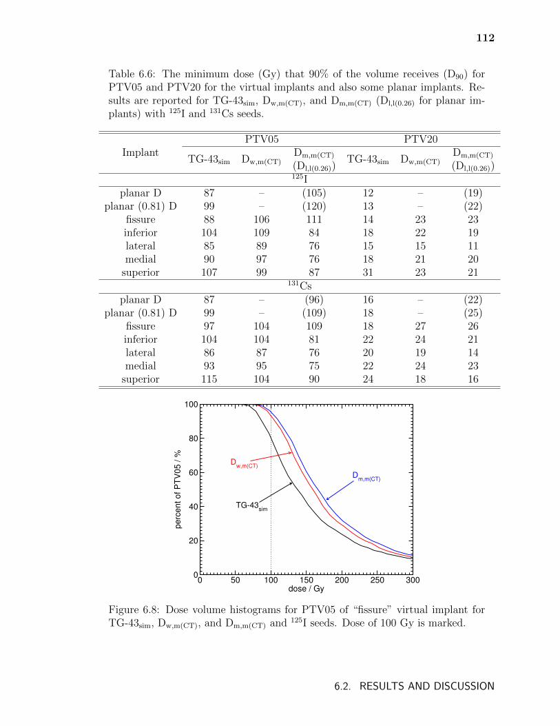
112
Table 6.6: The minimum dose (Gy) that 90% of the volume receives (D90) forPTV05 and PTV20 for the virtual implants and also some planar implants. Re-sults are reported for TG-43sim, Dw,m(CT), and Dm,m(CT) (Dl,l(0.26) for planar im-plants) with 125I and 131Cs seeds.
ImplantPTV05 PTV20
TG-43sim Dw,m(CT)Dm,m(CT) TG-43sim Dw,m(CT)
Dm,m(CT)
(Dl,l(0.26)) (Dl,l(0.26))125I
planar D 87 – (105) 12 – (19)planar (0.81) D 99 – (120) 13 – (22)
fissure 88 106 111 14 23 23inferior 104 109 84 18 22 19lateral 85 89 76 15 15 11medial 90 97 76 18 21 20
superior 107 99 87 31 23 21131Cs
planar D 87 – (96) 16 – (22)planar (0.81) D 99 – (109) 18 – (25)
fissure 97 104 109 18 27 26inferior 104 104 81 22 24 21lateral 86 87 76 20 19 14medial 93 95 75 22 24 23
superior 115 104 90 24 18 16
0 50 100 150 200 250 300dose / Gy
0
20
40
60
80
100
pe
rce
nt
of
PT
V0
5 /
%
TG-43sim
Dw,m(CT)
Dm,m(CT)
Figure 6.8: Dose volume histograms for PTV05 of “fissure” virtual implant forTG-43sim, Dw,m(CT), and Dm,m(CT) and 125I seeds. Dose of 100 Gy is marked.
6.2. RESULTS AND DISCUSSION
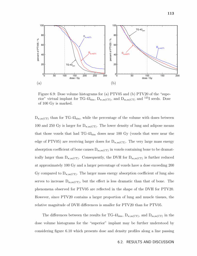
113
0 50 100 150 200 250 300dose / Gy
0
20
40
60
80
100
perc
ent of P
TV
05 / %
TG-43sim
Dw,m(CT)
Dm,m(CT)
0 50 100 150 200dose / Gy
0
20
40
60
80
100
perc
ent of P
TV
20 / %
TG-43sim
Dm,m(CT)
Dw,m(CT)
(a) (b)
Figure 6.9: Dose volume histograms for (a) PTV05 and (b) PTV20 of the “supe-rior” virtual implant for TG-43sim, Dw,m(CT), and Dm,m(CT) and 125I seeds. Doseof 100 Gy is marked.
Dw,m(CT) than for TG-43sim, while the percentage of the volume with doses between
100 and 250 Gy is larger for Dw,m(CT). The lower density of lung and adipose means
that those voxels that had TG-43sim doses near 100 Gy (voxels that were near the
edge of PTV05) are receiving larger doses for Dw,m(CT). The very large mass energy
absorption coefficient of bone causes Dm,m(CT) in voxels containing bone to be dramat-
ically larger than Dw,m(CT). Consequently, the DVH for Dm,m(CT) is further reduced
at approximately 100 Gy and a larger percentage of voxels have a dose exceeding 200
Gy compared to Dw,m(CT). The larger mass energy absorption coefficient of lung also
serves to increase Dm,m(CT), but the effect is less dramatic than that of bone. The
phenomena observed for PTV05 are reflected in the shape of the DVH for PTV20.
However, since PTV20 contains a larger proportion of lung and muscle tissues, the
relative magnitude of DVH differences is smaller for PTV20 than for PTV05.
The differences between the results for TG-43sim, Dw,m(CT), and Dm,m(CT) in the
dose volume histograms for the “superior” implant may be further understood by
considering figure 6.10 which presents dose and density profiles along a line passing
6.2. RESULTS AND DISCUSSION
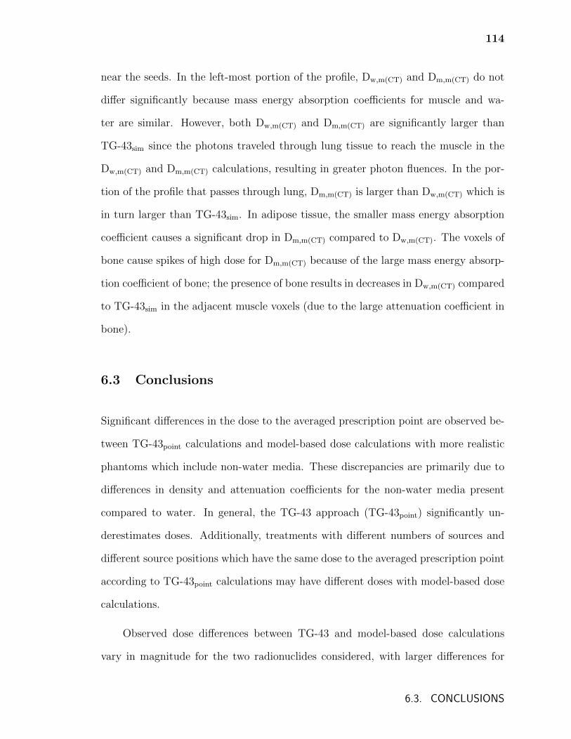
114
near the seeds. In the left-most portion of the profile, Dw,m(CT) and Dm,m(CT) do not
differ significantly because mass energy absorption coefficients for muscle and wa-
ter are similar. However, both Dw,m(CT) and Dm,m(CT) are significantly larger than
TG-43sim since the photons traveled through lung tissue to reach the muscle in the
Dw,m(CT) and Dm,m(CT) calculations, resulting in greater photon fluences. In the por-
tion of the profile that passes through lung, Dm,m(CT) is larger than Dw,m(CT) which is
in turn larger than TG-43sim. In adipose tissue, the smaller mass energy absorption
coefficient causes a significant drop in Dm,m(CT) compared to Dw,m(CT). The voxels of
bone cause spikes of high dose for Dm,m(CT) because of the large mass energy absorp-
tion coefficient of bone; the presence of bone results in decreases in Dw,m(CT) compared
to TG-43sim in the adjacent muscle voxels (due to the large attenuation coefficient in
bone).
6.3 Conclusions
Significant differences in the dose to the averaged prescription point are observed be-
tween TG-43point calculations and model-based dose calculations with more realistic
phantoms which include non-water media. These discrepancies are primarily due to
differences in density and attenuation coefficients for the non-water media present
compared to water. In general, the TG-43 approach (TG-43point) significantly un-
derestimates doses. Additionally, treatments with different numbers of sources and
different source positions which have the same dose to the averaged prescription point
according to TG-43point calculations may have different doses with model-based dose
calculations.
Observed dose differences between TG-43 and model-based dose calculations
vary in magnitude for the two radionuclides considered, with larger differences for
6.3. CONCLUSIONS
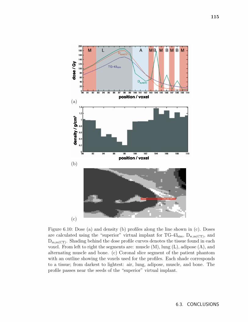
115
position / voxel
dose
/ G
y
(a)
dens
ity /
g/cm
3
position / voxel(b)
(c)
Figure 6.10: Dose (a) and density (b) profiles along the line shown in (c). Dosesare calculated using the “superior” virtual implant for TG-43sim, Dw,m(CT), andDm,m(CT). Shading behind the dose profile curves denotes the tissue found in eachvoxel. From left to right the segments are: muscle (M), lung (L), adipose (A), andalternating muscle and bone. (c) Coronal slice segment of the patient phantomwith an outline showing the voxels used for the profiles. Each shade correspondsto a tissue; from darkest to lightest: air, lung, adipose, muscle, and bone. Theprofile passes near the seeds of the “superior” virtual implant.
6.3. CONCLUSIONS
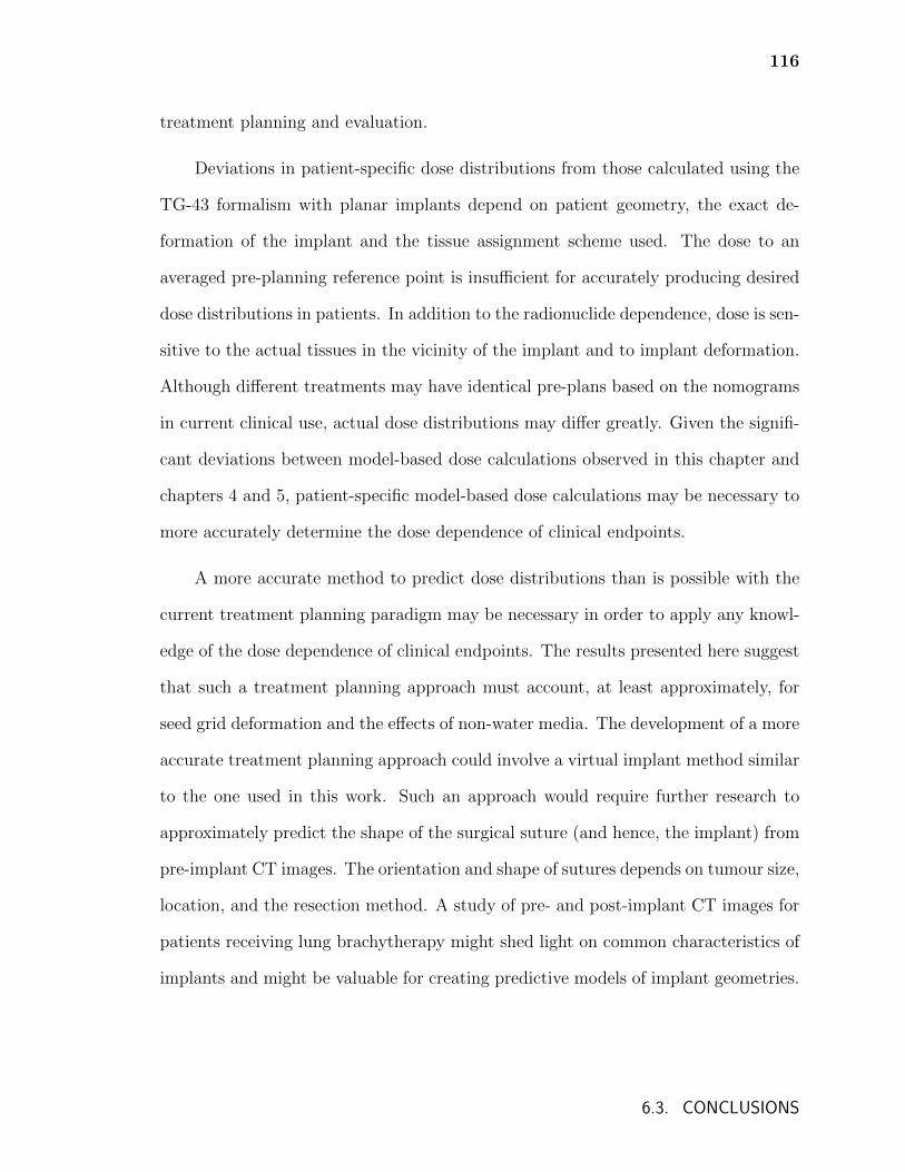
116
treatment planning and evaluation.
Deviations in patient-specific dose distributions from those calculated using the
TG-43 formalism with planar implants depend on patient geometry, the exact de-
formation of the implant and the tissue assignment scheme used. The dose to an
averaged pre-planning reference point is insufficient for accurately producing desired
dose distributions in patients. In addition to the radionuclide dependence, dose is sen-
sitive to the actual tissues in the vicinity of the implant and to implant deformation.
Although different treatments may have identical pre-plans based on the nomograms
in current clinical use, actual dose distributions may differ greatly. Given the signifi-
cant deviations between model-based dose calculations observed in this chapter and
chapters 4 and 5, patient-specific model-based dose calculations may be necessary to
more accurately determine the dose dependence of clinical endpoints.
A more accurate method to predict dose distributions than is possible with the
current treatment planning paradigm may be necessary in order to apply any knowl-
edge of the dose dependence of clinical endpoints. The results presented here suggest
that such a treatment planning approach must account, at least approximately, for
seed grid deformation and the effects of non-water media. The development of a more
accurate treatment planning approach could involve a virtual implant method similar
to the one used in this work. Such an approach would require further research to
approximately predict the shape of the surgical suture (and hence, the implant) from
pre-implant CT images. The orientation and shape of sutures depends on tumour size,
location, and the resection method. A study of pre- and post-implant CT images for
patients receiving lung brachytherapy might shed light on common characteristics of
implants and might be valuable for creating predictive models of implant geometries.
6.3. CONCLUSIONS

Chapter 7
Monte Carlo calculated doses to treatment
volumes and organs at risk for permanent
implant lung brachytherapy
While treatments for permanent implant lung brachytherapy have currently only been
reported for 125I and 131Cs implants21,114, the use of 169Yb surgical staples is being
investigated (Ref. 22), 103Pd has been used in the treatment of stage III NSCLC115,
and the use of novel radionuclides continues to be investigated for brachytherapy in
general116.
Yang and Rivard55 calculated dose distributions using a simplified lung geometry
with monoenergetic point sources of various energies and found considerable differ-
ences between TG-43 and Monte Carlo calculated doses. This thesis has presented
considerable differences between TG-43 and Monte Carlo calculated dose distributions
for post-treatment patient specific calculations (chapter 4), pre-planning prescription
dose calculations (chapter 6), as well as differences between patient specific Monte
Carlo calculated dose distributions using different radionuclides (chapter 6). Addi-
tionally, chapter 6 showed that the deformation of implants and variations in tissues
in the vicinity of implants were found to considerably affect dose distributions. These
effects varied in magnitude for 125I and 131Cs seeds, suggesting that doses to pa-
117
118
tient treatment volumes are sensitive to the choice of radionuclide, independent of
prescription doses.
The literature for permanent implant lung brachytherapy has made only sparse
mention of doses to healthy tissues. A study of the dose to intrathoracic organs
was reported117 but dose calculations were performed using the TG-43 formalism.
Additionally, while 125I lung brachytherapy has been reported to be safe with vir-
tually no increased morbidity17, some patients may be excluded as candidates for
brachytherapy or prescription doses may be lowered due to concern for healthy tis-
sues21. Doses to healthy tissues will be sensitive to the photon energy spectra of the
radionuclide used and differences in dose due to photon energy spectra are likely to
be misrepresented by water-based calculations. Consequently, accurate model-based
dose calculations are important for understanding how to safely and effectively adopt
new radionuclides and to better inform the current use of 125I and 131Cs sources in
lung brachytherapy.
This chapter investigates dosimetry for permanent implant lung brachytherapy
considering a range of source energies and various implant sites in the lung. Doses
to treatment volumes as well as the ipsilateral lung, heart, and aorta are studied.
Monte Carlo calculations are performed for a variety of virtual implants generated
using patient lung contours (see section 6.1.2, page 99) and using a computational
phantom derived from patient CT and organ-contour data. Dose distributions are
calculated for 103Pd, 125I, and 131Cs seeds as well as for 50 and 100 keV monoenergetic
point sources in the computational phantom and in a homogeneous water phantom
with no interseed attenuation to approximate TG-43 calculations. Dose metrics for
the heart, aorta, and lung as well as virtual treatment volumes are compared.
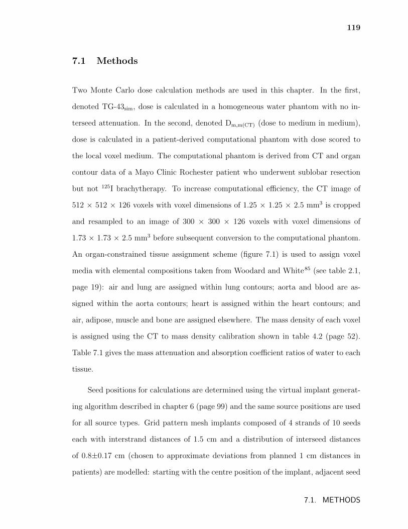
119
7.1 Methods
Two Monte Carlo dose calculation methods are used in this chapter. In the first,
denoted TG-43sim, dose is calculated in a homogeneous water phantom with no in-
terseed attenuation. In the second, denoted Dm,m(CT) (dose to medium in medium),
dose is calculated in a patient-derived computational phantom with dose scored to
the local voxel medium. The computational phantom is derived from CT and organ
contour data of a Mayo Clinic Rochester patient who underwent sublobar resection
but not 125I brachytherapy. To increase computational efficiency, the CT image of
512 × 512 × 126 voxels with voxel dimensions of 1.25 × 1.25 × 2.5 mm3 is cropped
and resampled to an image of 300 × 300 × 126 voxels with voxel dimensions of
1.73 × 1.73 × 2.5 mm3 before subsequent conversion to the computational phantom.
An organ-constrained tissue assignment scheme (figure 7.1) is used to assign voxel
media with elemental compositions taken from Woodard and White85 (see table 2.1,
page 19): air and lung are assigned within lung contours; aorta and blood are as-
signed within the aorta contours; heart is assigned within the heart contours; and
air, adipose, muscle and bone are assigned elsewhere. The mass density of each voxel
is assigned using the CT to mass density calibration shown in table 4.2 (page 52).
Table 7.1 gives the mass attenuation and absorption coefficient ratios of water to each
tissue.
Seed positions for calculations are determined using the virtual implant generat-
ing algorithm described in chapter 6 (page 99) and the same source positions are used
for all source types. Grid pattern mesh implants composed of 4 strands of 10 seeds
each with interstrand distances of 1.5 cm and a distribution of interseed distances
of 0.8±0.17 cm (chosen to approximate deviations from planned 1 cm distances in
patients) are modelled: starting with the centre position of the implant, adjacent seed
7.1. METHODS
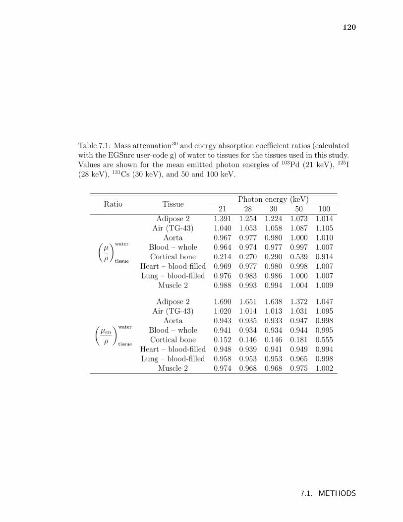
120
Table 7.1: Mass attenuation30 and energy absorption coefficient ratios (calculatedwith the EGSnrc user-code g) of water to tissues for the tissues used in this study.Values are shown for the mean emitted photon energies of 103Pd (21 keV), 125I(28 keV), 131Cs (30 keV), and 50 and 100 keV.
Ratio TissuePhoton energy (keV)
21 28 30 50 100
(µ
ρ
)water
tissue
Adipose 2 1.391 1.254 1.224 1.073 1.014Air (TG-43) 1.040 1.053 1.058 1.087 1.105
Aorta 0.967 0.977 0.980 1.000 1.010Blood – whole 0.964 0.974 0.977 0.997 1.007Cortical bone 0.214 0.270 0.290 0.539 0.914
Heart – blood-filled 0.969 0.977 0.980 0.998 1.007Lung – blood-filled 0.976 0.983 0.986 1.000 1.007
Muscle 2 0.988 0.993 0.994 1.004 1.009
(µenρ
)water
tissue
Adipose 2 1.690 1.651 1.638 1.372 1.047Air (TG-43) 1.020 1.014 1.013 1.031 1.095
Aorta 0.943 0.935 0.933 0.947 0.998Blood – whole 0.941 0.934 0.934 0.944 0.995Cortical bone 0.152 0.146 0.146 0.181 0.555
Heart – blood-filled 0.948 0.939 0.941 0.949 0.994Lung – blood-filled 0.958 0.953 0.953 0.965 0.998
Muscle 2 0.974 0.968 0.968 0.975 1.002
7.1. METHODS
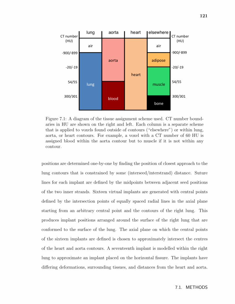
121
Figure 7.1: A diagram of the tissue assignment scheme used. CT number bound-aries in HU are shown on the right and left. Each column is a separate schemethat is applied to voxels found outside of contours (“elsewhere”) or within lung,aorta, or heart contours. For example, a voxel with a CT number of 60 HU isassigned blood within the aorta contour but to muscle if it is not within anycontour.
positions are determined one-by-one by finding the position of closest approach to the
lung contours that is constrained by some (interseed/interstrand) distance. Suture
lines for each implant are defined by the midpoints between adjacent seed positions
of the two inner strands. Sixteen virtual implants are generated with central points
defined by the intersection points of equally spaced radial lines in the axial plane
starting from an arbitrary central point and the contours of the right lung. This
produces implant positions arranged around the surface of the right lung that are
conformed to the surface of the lung. The axial plane on which the central points
of the sixteen implants are defined is chosen to approximately intersect the centres
of the heart and aorta contours. A seventeenth implant is modelled within the right
lung to approximate an implant placed on the horizontal fissure. The implants have
differing deformations, surrounding tissues, and distances from the heart and aorta.
7.1. METHODS
122
Figure 7.2 shows points indicating the centres of each virtual implant overlaid on a
slice of the patient CT image, as well as contours for the heart and aorta. As an
example, figure 7.3 shows implant number 1 and the contours of the right lung.
Figure 7.2: A slice of the CT image for the Mayo Clinic patient view from aninferior position. Heart (upper) and aorta (lower) contours are shown. Thepositions of the centres of the virtual implants in the right lung are marked andnumbered 1-17. Implant 17 is modelled as an implant placed on the horizontalfissure. Two implant positions in the left lung (labelled ”a” and ”b”) are alsoindicated.
Five source models are considered for this study: 103Pd (mean emitted photon
energy of the radionuclide, Eγ = 21 keV) Theragenics Co. (Buford Georgia USA)
TheraSeed 200, 125I (Eγ = 28 keV) GE Healthcare/Oncura (Arlington Heights IL
USA) model 6711, 131Cs (Eγ = 30 keV) IsoRay (Richland WA USA) CS-1 Rev2, as
well as 50 and 100 keV monoenergetic point sources. Monoenergetic sources are used
7.1. METHODS
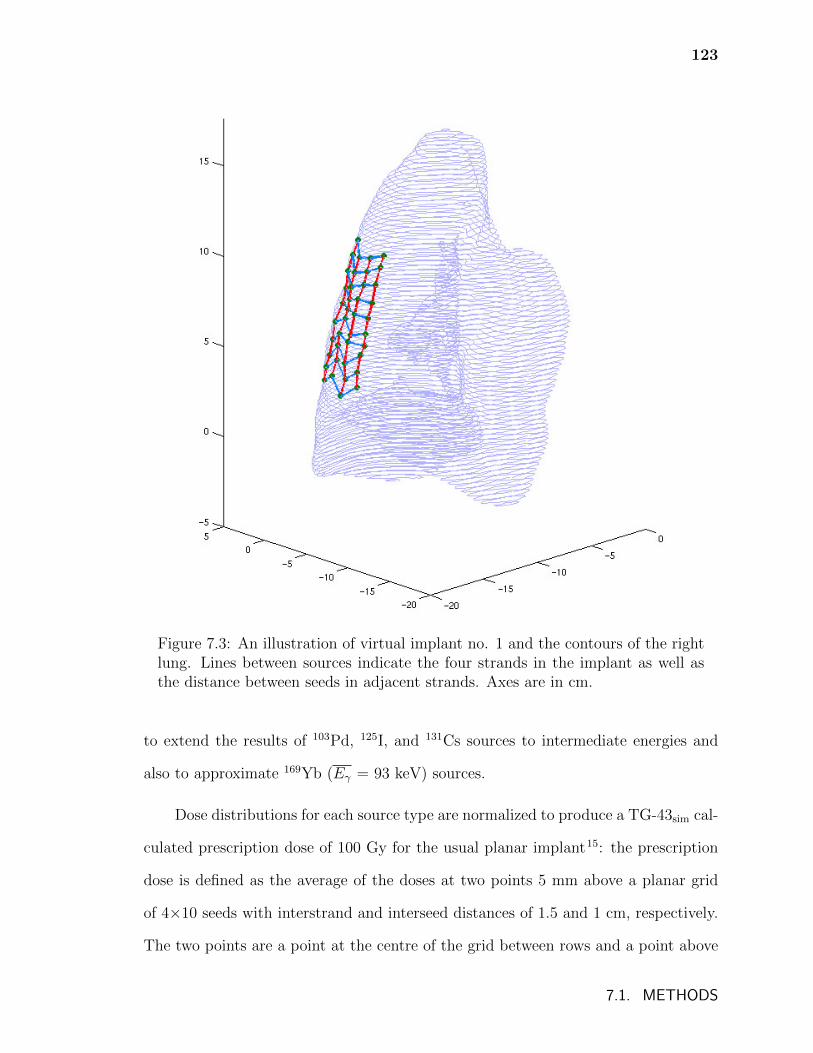
123
Figure 7.3: An illustration of virtual implant no. 1 and the contours of the rightlung. Lines between sources indicate the four strands in the implant as well asthe distance between seeds in adjacent strands. Axes are in cm.
to extend the results of 103Pd, 125I, and 131Cs sources to intermediate energies and
also to approximate 169Yb (Eγ = 93 keV) sources.
Dose distributions for each source type are normalized to produce a TG-43sim cal-
culated prescription dose of 100 Gy for the usual planar implant15: the prescription
dose is defined as the average of the doses at two points 5 mm above a planar grid
of 4×10 seeds with interstrand and interseed distances of 1.5 and 1 cm, respectively.
The two points are a point at the centre of the grid between rows and a point above
7.1. METHODS
124
a central row of seeds at the centre of the row (see chapter 6, page 97). An arbitrary
prescription dose of 100 Gy, while unrealistic for sources other than 125I, facilitates
comparison between source types and results in each dose also being equivalent to
the percentage of an arbitrary prescription dose (%DRx).
Dose metrics are reported for heart, aorta, and ipsilateral (right) lung volumes
as well as for PTV05 and PTV20 treatment volumes which are defined as 5 mm and
20 mm expansions of suture lines, respectively. The whole heart volume is contoured
and the aorta contours delineate 7 cm of the descending aorta. Mean doses to the
aorta and heart, as well as the heart volume that receives at least 5 Gy (V5) are
calculated. Dose volume histograms (DVHs) for the fissure implants (position no.
17) and mean doses for all of the implants are calculated for the ipsilateral (right)
lung volume. For PTV05 and PTV20, the minimum doses received by the hottest 90%
of the volumes (D90) and the percentages of the volumes that receive at least 100 Gy
(V100 or, equivalently, VDRx) and 200 Gy (V200) are calculated. Calculations, taking
approximately 240 CPU hours on a single 3.0 GHz Woodcrest core are performed
with 5×10¹⁰ histories to achieve a maximum statistical uncertainty of 0.4% in PTV20
volumes for 103Pd calculations (with lower uncertainties achieved for other sources).
7.2 Results and Discussion
7.2.1 Doses to treatment volumes
D90 for PTV05 and PTV20 for the various implants and radionuclides can be seen in
figure 7.4. Values of D90 for Dm,m(CT) vary between implants and range between 40 –
150 Gy and 7 – 45 Gy for PTV05 and PTV20, respectively. The range of D90 values
for TG-43sim is comparable but somewhat smaller: 35 – 120 Gy for PTV05 and 13 –
7.2. RESULTS AND DISCUSSION
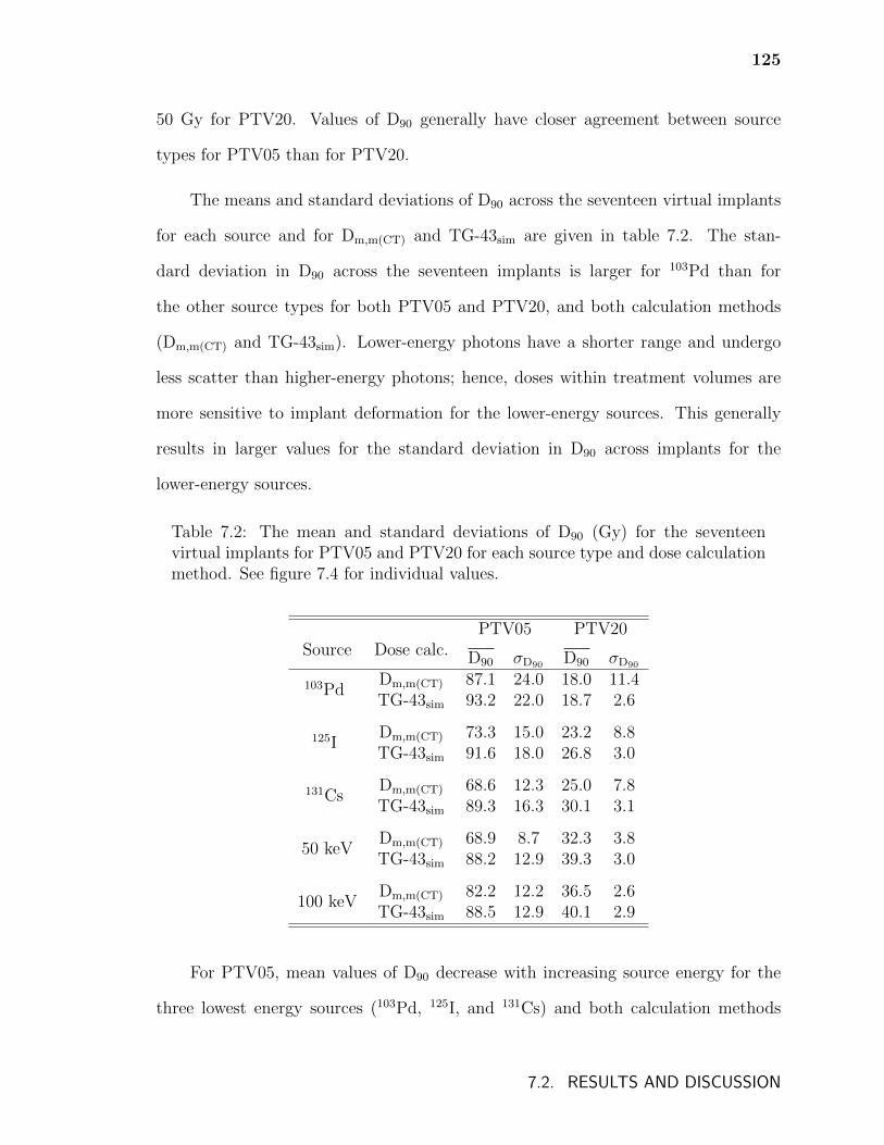
125
50 Gy for PTV20. Values of D90 generally have closer agreement between source
types for PTV05 than for PTV20.
The means and standard deviations of D90 across the seventeen virtual implants
for each source and for Dm,m(CT) and TG-43sim are given in table 7.2. The stan-
dard deviation in D90 across the seventeen implants is larger for 103Pd than for
the other source types for both PTV05 and PTV20, and both calculation methods
(Dm,m(CT) and TG-43sim). Lower-energy photons have a shorter range and undergo
less scatter than higher-energy photons; hence, doses within treatment volumes are
more sensitive to implant deformation for the lower-energy sources. This generally
results in larger values for the standard deviation in D90 across implants for the
lower-energy sources.
Table 7.2: The mean and standard deviations of D90 (Gy) for the seventeenvirtual implants for PTV05 and PTV20 for each source type and dose calculationmethod. See figure 7.4 for individual values.
Source Dose calc.PTV05 PTV20
D90 σD90 D90 σD90
103PdDm,m(CT) 87.1 24.0 18.0 11.4TG-43sim 93.2 22.0 18.7 2.6
125IDm,m(CT) 73.3 15.0 23.2 8.8TG-43sim 91.6 18.0 26.8 3.0
131CsDm,m(CT) 68.6 12.3 25.0 7.8TG-43sim 89.3 16.3 30.1 3.1
50 keVDm,m(CT) 68.9 8.7 32.3 3.8TG-43sim 88.2 12.9 39.3 3.0
100 keVDm,m(CT) 82.2 12.2 36.5 2.6TG-43sim 88.5 12.9 40.1 2.9
For PTV05, mean values of D90 decrease with increasing source energy for the
three lowest energy sources (103Pd, 125I, and 131Cs) and both calculation methods
7.2. RESULTS AND DISCUSSION
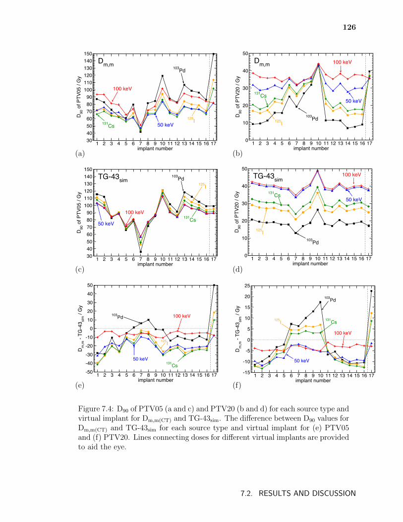
126
1 2 3 4 5 6 7 8 9 10 11 12 13 14 15 16 17implant number
30405060708090
100110120130140150
D90
of P
TV05
/ G
y
Dm,m103Pd
100 keV
50 keV131Cs125I
1 2 3 4 5 6 7 8 9 10 11 12 13 14 15 16 17implant number
0
10
20
30
40
50
D90
of P
TV20
/ G
y
103Pd
100 keV
50 keV131Cs
125I
Dm,m
(a) (b)
1 2 3 4 5 6 7 8 9 10 11 12 13 14 15 16 17implant number
30405060708090
100110120130140150
D90
of P
TV05
/ G
y
TG-43sim103Pd
100 keV
50 keV131Cs
125I
1 2 3 4 5 6 7 8 9 10 11 12 13 14 15 16 17implant number
0
10
20
30
40
50
D90
of P
TV20
/ G
y103Pd
100 keV
50 keV131Cs
125I
TG-43sim
(c) (d)
1 2 3 4 5 6 7 8 9 10 11 12 13 14 15 16 17implant number
-50
-40
-30
-20
-10
0
10
20
30
40
50
Dm
,m -
TG-4
3 sim
/ G
y
103Pd 100 keV
131Cs
125I
50 keV
1 2 3 4 5 6 7 8 9 10 11 12 13 14 15 16 17implant number
-15
-10
-5
0
5
10
15
20
25
Dm
,m -
TG-4
3 sim
/ G
y
103Pd
125I 131Cs
50 keV
100 keV
(e) (f)
Figure 7.4: D90 of PTV05 (a and c) and PTV20 (b and d) for each source type andvirtual implant for Dm,m(CT) and TG-43sim. The difference between D90 values forDm,m(CT) and TG-43sim for each source type and virtual implant for (e) PTV05and (f) PTV20. Lines connecting doses for different virtual implants are providedto aid the eye.
7.2. RESULTS AND DISCUSSION
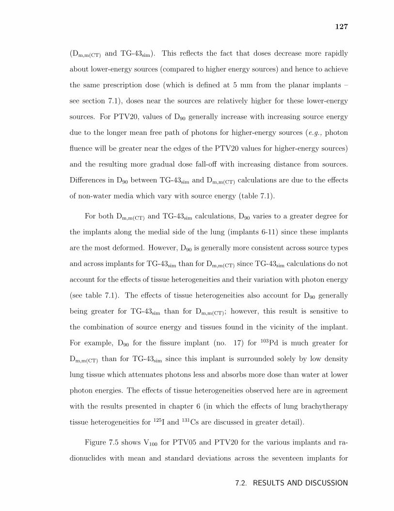
127
(Dm,m(CT) and TG-43sim). This reflects the fact that doses decrease more rapidly
about lower-energy sources (compared to higher energy sources) and hence to achieve
the same prescription dose (which is defined at 5 mm from the planar implants –
see section 7.1), doses near the sources are relatively higher for these lower-energy
sources. For PTV20, values of D90 generally increase with increasing source energy
due to the longer mean free path of photons for higher-energy sources (e.g., photon
fluence will be greater near the edges of the PTV20 values for higher-energy sources)
and the resulting more gradual dose fall-off with increasing distance from sources.
Differences in D90 between TG-43sim and Dm,m(CT) calculations are due to the effects
of non-water media which vary with source energy (table 7.1).
For both Dm,m(CT) and TG-43sim calculations, D90 varies to a greater degree for
the implants along the medial side of the lung (implants 6-11) since these implants
are the most deformed. However, D90 is generally more consistent across source types
and across implants for TG-43sim than for Dm,m(CT) since TG-43sim calculations do not
account for the effects of tissue heterogeneities and their variation with photon energy
(see table 7.1). The effects of tissue heterogeneities also account for D90 generally
being greater for TG-43sim than for Dm,m(CT); however, this result is sensitive to
the combination of source energy and tissues found in the vicinity of the implant.
For example, D90 for the fissure implant (no. 17) for 103Pd is much greater for
Dm,m(CT) than for TG-43sim since this implant is surrounded solely by low density
lung tissue which attenuates photons less and absorbs more dose than water at lower
photon energies. The effects of tissue heterogeneities observed here are in agreement
with the results presented in chapter 6 (in which the effects of lung brachytherapy
tissue heterogeneities for 125I and 131Cs are discussed in greater detail).
Figure 7.5 shows V100 for PTV05 and PTV20 for the various implants and ra-
dionuclides with mean and standard deviations across the seventeen implants for
7.2. RESULTS AND DISCUSSION
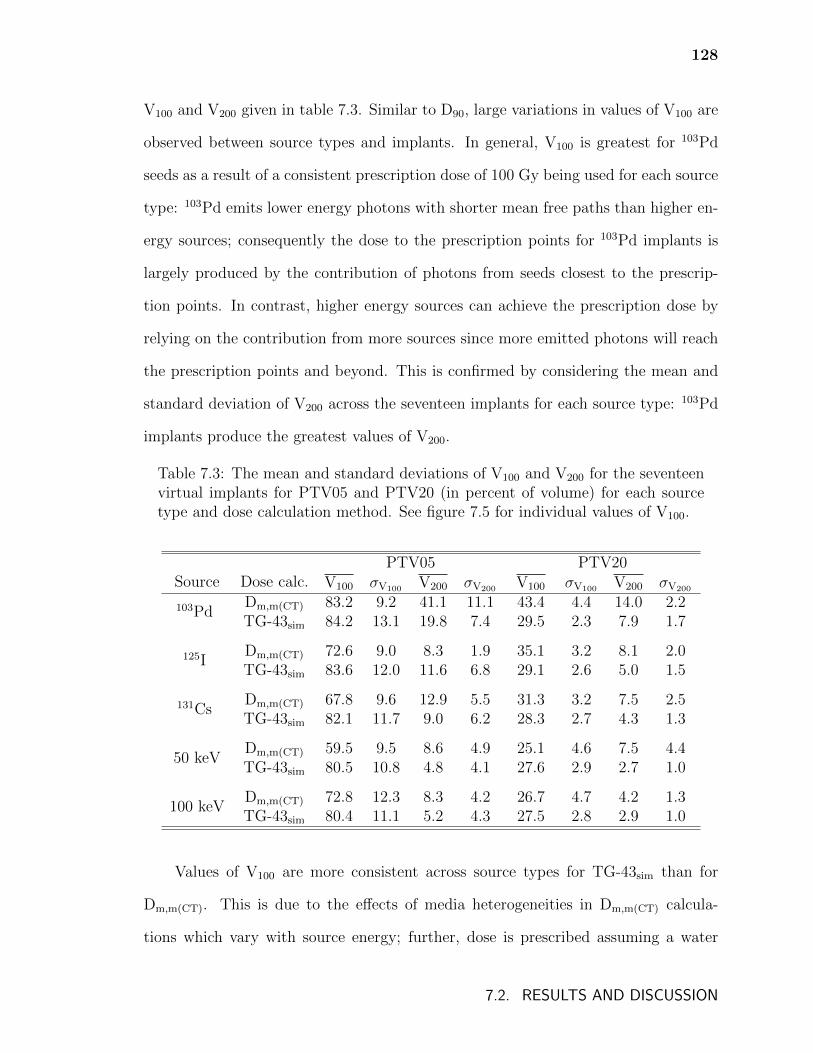
128
V100 and V200 given in table 7.3. Similar to D90, large variations in values of V100 are
observed between source types and implants. In general, V100 is greatest for 103Pd
seeds as a result of a consistent prescription dose of 100 Gy being used for each source
type: 103Pd emits lower energy photons with shorter mean free paths than higher en-
ergy sources; consequently the dose to the prescription points for 103Pd implants is
largely produced by the contribution of photons from seeds closest to the prescrip-
tion points. In contrast, higher energy sources can achieve the prescription dose by
relying on the contribution from more sources since more emitted photons will reach
the prescription points and beyond. This is confirmed by considering the mean and
standard deviation of V200 across the seventeen implants for each source type: 103Pd
implants produce the greatest values of V200.
Table 7.3: The mean and standard deviations of V100 and V200 for the seventeenvirtual implants for PTV05 and PTV20 (in percent of volume) for each sourcetype and dose calculation method. See figure 7.5 for individual values of V100.
Source Dose calc.PTV05 PTV20
V100 σV100 V200 σV200 V100 σV100 V200 σV200
103PdDm,m(CT) 83.2 9.2 41.1 11.1 43.4 4.4 14.0 2.2TG-43sim 84.2 13.1 19.8 7.4 29.5 2.3 7.9 1.7
125IDm,m(CT) 72.6 9.0 8.3 1.9 35.1 3.2 8.1 2.0TG-43sim 83.6 12.0 11.6 6.8 29.1 2.6 5.0 1.5
131CsDm,m(CT) 67.8 9.6 12.9 5.5 31.3 3.2 7.5 2.5TG-43sim 82.1 11.7 9.0 6.2 28.3 2.7 4.3 1.3
50 keVDm,m(CT) 59.5 9.5 8.6 4.9 25.1 4.6 7.5 4.4TG-43sim 80.5 10.8 4.8 4.1 27.6 2.9 2.7 1.0
100 keVDm,m(CT) 72.8 12.3 8.3 4.2 26.7 4.7 4.2 1.3TG-43sim 80.4 11.1 5.2 4.3 27.5 2.8 2.9 1.0
Values of V100 are more consistent across source types for TG-43sim than for
Dm,m(CT). This is due to the effects of media heterogeneities in Dm,m(CT) calcula-
tions which vary with source energy; further, dose is prescribed assuming a water
7.2. RESULTS AND DISCUSSION
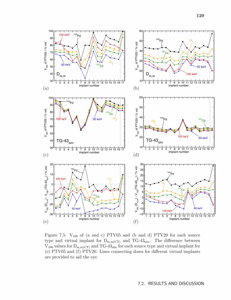
129
1 2 3 4 5 6 7 8 9 10 11 12 13 14 15 16 17implant number
30
40
50
60
70
80
90
100
V 100 o
f PTV
05 /
% v
ol.
Dm,m
103Pd100 keV
50 keV 131Cs125I
1 2 3 4 5 6 7 8 9 10 11 12 13 14 15 16 17implant number
10
20
30
40
50
60
V 100 o
f PTV
20 /
% v
ol.
Dm,m
103Pd
50 keV
125I
131Cs
100 keV
(a) (b)
1 2 3 4 5 6 7 8 9 10 11 12 13 14 15 16 17implant number
30
40
50
60
70
80
90
100
V 100 o
f PTV
05 /
% v
ol.
TG-43sim
103Pd
100 keV 50 keV
131Cs125I
1 2 3 4 5 6 7 8 9 10 11 12 13 14 15 16 17implant number
10
20
30
40
50
60
V 100 o
f PTV
20 /
% v
ol.
TG-43sim
103Pd125I
100 keV 50 keV
131Cs
(c) (d)
1 2 3 4 5 6 7 8 9 10 11 12 13 14 15 16 17implant number
-30
-20
-10
0
10
20
V 100 (D
m,m
) - V
100 (T
G-4
3 sim
) / %
vol
.
103Pd
100 keV 125I
50 keV
131Cs
1 2 3 4 5 6 7 8 9 10 11 12 13 14 15 16 17implant number
-15
-10
-5
0
5
10
15
20
25
30
V 100 (D
m,m
) - V
100(T
G-4
3 sim
) / %
vol
.
103Pd
125I131Cs
50 keV100 keV
(e) (f)
Figure 7.5: V100 of (a and c) PTV05 and (b and d) PTV20 for each sourcetype and virtual implant for Dm,m(CT) and TG-43sim. The difference betweenV100 values for Dm,m(CT) and TG-43sim for each source type and virtual implant for(e) PTV05 and (f) PTV20. Lines connecting doses for different virtual implantsare provided to aid the eye.
7.2. RESULTS AND DISCUSSION
130
environment (and ignoring the effects of non-water media). The effects of tissue
heterogeneities generally result in larger values of V100 for TG-43sim compared to
Dm,m(CT) for PTV05; for PTV20, values of V100 for TG-43sim are generally less than
or similar to those for Dm,m(CT).
For 103Pd, 125I, and 131Cs sources, Dm,m(CT) values of V100 are greater for implant
17 compared to other implants since implant 17 is surrounded solely by lung. The
reduced attenuation in lung and increased energy absorption in lung tissue compared
to water for lower energy photons (table 7.1) result in these relatively large values of
V100 for Dm,m(CT) compared to TG-43sim. Mass attenuation and absorption coefficient
ratios of water to lung are closer to unity for 50 keV and 100 keV photons (table 7.1)
and so these sources have lower values of V100 for Dm,m(CT) compared to TG-43sim due
to a reduced contribution of dose from back-scattered photons.
Actual patient implants will differ from the virtual implants considered in this
study due to varying resection sites and source implantation methods. However, the
results presented in this section demonstrate that treatment volume dose metrics vary
considerably with implant site and source type for both Dm,m(CT) and TG-43sim cal-
culations. These variations are due to the combined effects of implant deformation,
source energy, and tissues near the implant site (Dm,m(CT) only); studying each effect
in isolation dose not enable prediction of dose metrics for arbitrary treatment sites.
7.2.2 Doses to the right lung
Figure 7.6 shows the mean dose to the right lung for the seventeen implants and five
sources for Dm,m(CT) and TG-43sim. Mean lung doses range between a maximum value
of 27 Gy for 103Pd and Dm,m(CT) for implant 17 and a minimum of 6 Gy for 103Pd and
TG-43sim for implant 6. Differences between Dm,m(CT) and TG-43sim values of mean
7.2. RESULTS AND DISCUSSION
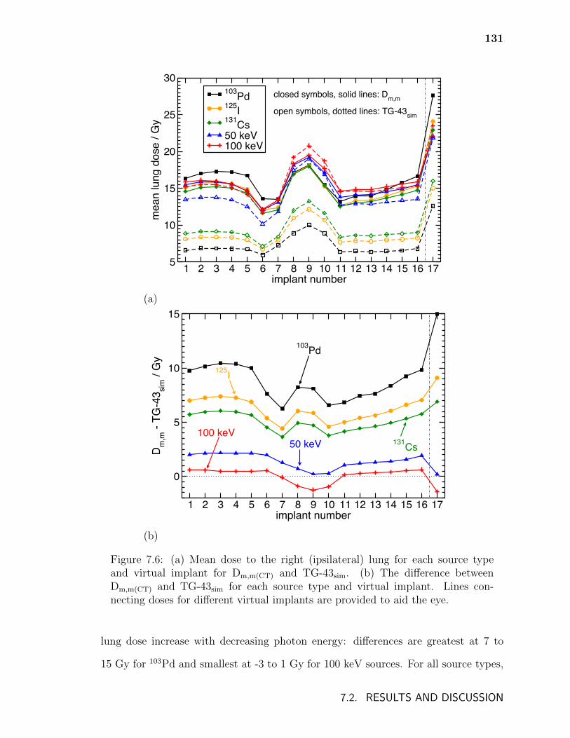
131
1 2 3 4 5 6 7 8 9 10 11 12 13 14 15 16 17implant number
5
10
15
20
25
30
mea
n lu
ng d
ose
/ Gy
103Pd125I131Cs50 keV100 keV
closed symbols, solid lines: Dm,m
open symbols, dotted lines: TG-43sim
(a)
1 2 3 4 5 6 7 8 9 10 11 12 13 14 15 16 17implant number
0
5
10
15
Dm
,m -
TG-4
3 sim
/ G
y
103Pd
125I
131Cs50 keV100 keV
(b)
Figure 7.6: (a) Mean dose to the right (ipsilateral) lung for each source typeand virtual implant for Dm,m(CT) and TG-43sim. (b) The difference betweenDm,m(CT) and TG-43sim for each source type and virtual implant. Lines con-necting doses for different virtual implants are provided to aid the eye.
lung dose increase with decreasing photon energy: differences are greatest at 7 to
15 Gy for 103Pd and smallest at -3 to 1 Gy for 100 keV sources. For all source types,
7.2. RESULTS AND DISCUSSION
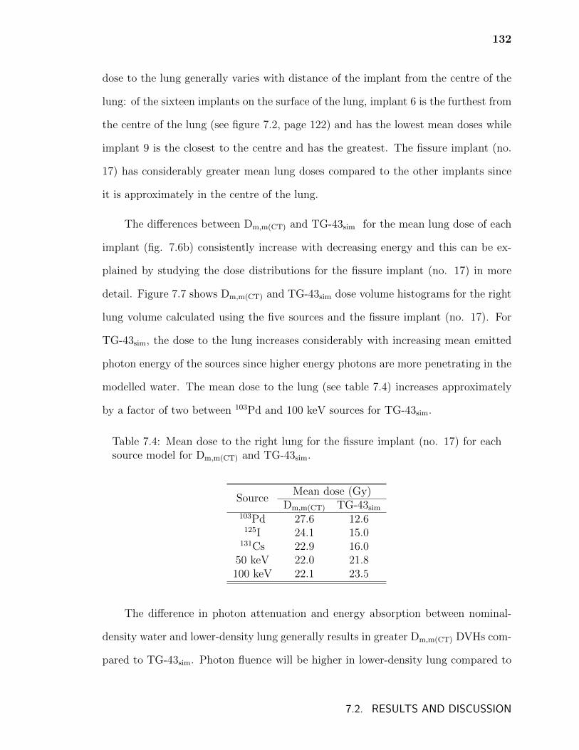
132
dose to the lung generally varies with distance of the implant from the centre of the
lung: of the sixteen implants on the surface of the lung, implant 6 is the furthest from
the centre of the lung (see figure 7.2, page 122) and has the lowest mean doses while
implant 9 is the closest to the centre and has the greatest. The fissure implant (no.
17) has considerably greater mean lung doses compared to the other implants since
it is approximately in the centre of the lung.
The differences between Dm,m(CT) and TG-43sim for the mean lung dose of each
implant (fig. 7.6b) consistently increase with decreasing energy and this can be ex-
plained by studying the dose distributions for the fissure implant (no. 17) in more
detail. Figure 7.7 shows Dm,m(CT) and TG-43sim dose volume histograms for the right
lung volume calculated using the five sources and the fissure implant (no. 17). For
TG-43sim, the dose to the lung increases considerably with increasing mean emitted
photon energy of the sources since higher energy photons are more penetrating in the
modelled water. The mean dose to the lung (see table 7.4) increases approximately
by a factor of two between 103Pd and 100 keV sources for TG-43sim.
Table 7.4: Mean dose to the right lung for the fissure implant (no. 17) for eachsource model for Dm,m(CT) and TG-43sim.
SourceMean dose (Gy)
Dm,m(CT) TG-43sim103Pd 27.6 12.6
125I 24.1 15.0131Cs 22.9 16.0
50 keV 22.0 21.8100 keV 22.1 23.5
The difference in photon attenuation and energy absorption between nominal-
density water and lower-density lung generally results in greater Dm,m(CT) DVHs com-
pared to TG-43sim. Photon fluence will be higher in lower-density lung compared to
7.2. RESULTS AND DISCUSSION
133
0 10 20 30 40 50dose / Gy
0
10
20
30
40
50
60
70
80
90
100
perc
enta
ge o
f lun
g vo
lum
e / %
103Pd
125I
131Cs100 keV
solid lines: Dm,mdashed lines: TG-43sim
125I131Cs
103Pd
50 keV
Figure 7.7: Dose volume histogram for the right lung for the fissure (no. 17)implant. DVHs for each radionuclide for Dm,m(CT) and TG-43sim are shown.
in water and this greater fluence combined with the greater mass energy absorp-
tion coefficients of lung compared to water (table 7.1) result in higher Dm,m(CT) than
TG-43sim for the lower-energy sources. As source energy increases, photon range
increases and the influence that scattered photons have on mean dose to the lung be-
comes more significant. Thus, as source energy increases, the effect of a lower photon
fluence in water compared to lung becomes reduced due to increased photon range
and is increasingly compensated by a greater proportion of photons being scattered
and contributing dose to the lung volume for TG-43sim compared to Dm,m(CT) where
photons may escape the lung and contribute no dose. For many implants (includ-
ing implant 17) the combined effects of differences in photon fluence and scattering
conditions causes the trend in mean lung dose with source energy to reverse: for
TG-43sim mean lung dose increases with source energy while it decreases with source
energy for Dm,m(CT).
7.2. RESULTS AND DISCUSSION
134
Marks et al.118 suggest that for external beam radiotherapy treatments of the
lung with conventional fractionation, V20 should be kept below 30-35% and that the
mean lung dose be kept below 20-23 Gy to limit the risk of symptomatic radiation
pneumonitis to less than or equal to 20%. These guidelines may not be appropriate
for brachytherapy due to radiobiological considerations (such as the effect of differ-
ences in dose rate and treatment length between brachytherapy and external beam
radiotherapy). Additionally, prescription doses for radionuclides other than 125I will
likely differ from the arbitrary 100 Gy used in this study. However, it is important
to note that, for the prescription dose used in this work, TG-43 calculations indicate
that lower energy sources produce lung doses well below the thresholds suggested by
Marks et al.118, while the doses determined by model-based, Dm,m(CT) calculations
are approximately equal to or greater than the thresholds. This underlines the im-
portance of model-based dose calculations for comparing different radionuclides in
low-energy brachytherapy.
7.2.3 Doses to the aorta
Figure 7.8a shows the mean aorta dose for each source type and virtual implant for
Dm,m(CT) and TG-43sim with differences between Dm,m(CT) and TG-43sim shown in
figure 7.8b. For 100 keV sources, doses range between approximately 1.5 – 11 Gy for
TG-43sim and between approximately 1.8 – 8 Gy for Dm,m(CT) while doses for both
TG-43sim and Dm,m(CT) stay below 0.5 Gy for 103Pd seeds. Mean dose to the aorta (as
a function of %DRX) increases with increasing mean emitted photon energy and there
is approximately an order of magnitude difference in mean aorta dose between 103Pd
and 100 keV sources for implants near the aorta (e.g., implant 10) since the higher
energy photons for 50 and 100 keV monoenergetic sources are more penetrating. For
implants on the lateral side of the lung, aorta doses are near zero for 103Pd, 125I, and
131Cs; however, aorta doses are non-zero for 50 keV and 100 keV sources.
7.2. RESULTS AND DISCUSSION

135
1 2 3 4 5 6 7 8 9 10 11 12 13 14 15 16 17implant number
0
2
4
6
8
10
12
mea
n ao
rta d
ose
/ Gy
103Pd125I131Cs50 keV100 keV
closed symbols, solid lines: Dm,m
open symbols, dotted lines: TG-43sim
(a)
1 2 3 4 5 6 7 8 9 10 11 12 13 14 15 16 17implant number
-4
-3
-2
-1
0
1
Dm
,m -
TG-4
3 sim
/ G
y
103Pd125I
131Cs
50 keV
100 keV
(b)
Figure 7.8: (a) The mean aorta dose for each source type and virtual implant forDm,m(CT) and TG-43sim. (b) The difference between Dm,m(CT) and TG-43sim foreach source type and virtual implant. . Lines connecting doses for differentvirtual implants are provided to aid the eye.
7.2. RESULTS AND DISCUSSION
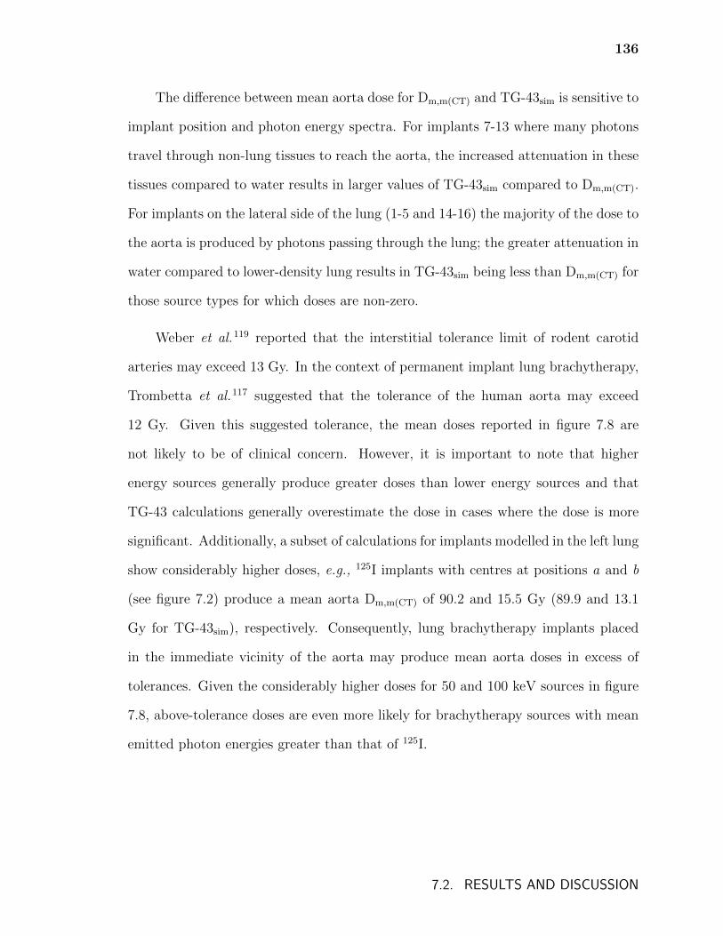
136
The difference between mean aorta dose for Dm,m(CT) and TG-43sim is sensitive to
implant position and photon energy spectra. For implants 7-13 where many photons
travel through non-lung tissues to reach the aorta, the increased attenuation in these
tissues compared to water results in larger values of TG-43sim compared to Dm,m(CT).
For implants on the lateral side of the lung (1-5 and 14-16) the majority of the dose to
the aorta is produced by photons passing through the lung; the greater attenuation in
water compared to lower-density lung results in TG-43sim being less than Dm,m(CT) for
those source types for which doses are non-zero.
Weber et al.119 reported that the interstitial tolerance limit of rodent carotid
arteries may exceed 13 Gy. In the context of permanent implant lung brachytherapy,
Trombetta et al.117 suggested that the tolerance of the human aorta may exceed
12 Gy. Given this suggested tolerance, the mean doses reported in figure 7.8 are
not likely to be of clinical concern. However, it is important to note that higher
energy sources generally produce greater doses than lower energy sources and that
TG-43 calculations generally overestimate the dose in cases where the dose is more
significant. Additionally, a subset of calculations for implants modelled in the left lung
show considerably higher doses, e.g., 125I implants with centres at positions a and b
(see figure 7.2) produce a mean aorta Dm,m(CT) of 90.2 and 15.5 Gy (89.9 and 13.1
Gy for TG-43sim), respectively. Consequently, lung brachytherapy implants placed
in the immediate vicinity of the aorta may produce mean aorta doses in excess of
tolerances. Given the considerably higher doses for 50 and 100 keV sources in figure
7.8, above-tolerance doses are even more likely for brachytherapy sources with mean
emitted photon energies greater than that of 125I.
7.2. RESULTS AND DISCUSSION
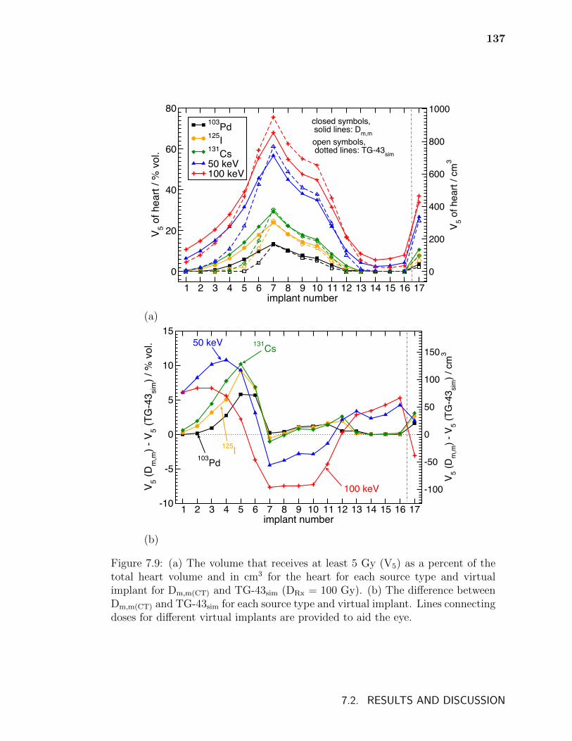
137
1 2 3 4 5 6 7 8 9 10 11 12 13 14 15 16 17implant number
0
20
40
60
80
V 5 of h
eart
/ % v
ol.
103Pd125I131Cs50 keV100 keV
0
200
400
600
800
1000
V 5 of h
eart
/ cm
3
closed symbols, solid lines: Dm,mopen symbols, dotted lines: TG-43sim
(a)
1 2 3 4 5 6 7 8 9 10 11 12 13 14 15 16 17implant number
-10
-5
0
5
10
15
V 5 (Dm
,m) -
V5 (T
G-4
3 sim
) / %
vol
.
-100
-50
0
50
100
150
V 5 (Dm
,m) -
V5 (T
G-4
3 sim
) / c
m3
100 keV
50 keV 131Cs
103Pd
125I
(b)
Figure 7.9: (a) The volume that receives at least 5 Gy (V5) as a percent of thetotal heart volume and in cm3 for the heart for each source type and virtualimplant for Dm,m(CT) and TG-43sim (DRx = 100 Gy). (b) The difference betweenDm,m(CT) and TG-43sim for each source type and virtual implant. Lines connectingdoses for different virtual implants are provided to aid the eye.
7.2. RESULTS AND DISCUSSION
138
7.2.4 Doses to the heart
Figure 7.9 shows V5 of the heart for the seventeen virtual implants and five source
types for Dm,m(CT) and TG-43sim. Values of V5 are greatest for 100 keV sources and
lowest for 103Pd with V5 values for 100 keV sources ranging between approximately
10 – 70 % for Dm,m(CT) and 5 – 75 % for TG-43sim and volumes for 103Pd ranging
between 0 – 12 % for both Dm,m(CT) and TG-43sim. For implants 7 and 8, V5 for
Dm,m(CT) and TG-43sim are in close agreement for 103Pd, 125I, and 131Cs implants while
for 50 and 100 keV implants, V5 is greater for TG-43sim than for Dm,m(CT) despite heart
having a greater mass energy absorption coefficient than water at these energies. This
is due to TG-43 calculations modelling more photons scattering in water for higher-
energy sources and contributing more dose in the organ at risk than in model-based
calculations where lower-density lung is modelled. For implants where photons must
travel through lung tissue before reaching the heart (eg. implants 1-5 and 13-16), V5 is
greater for Dm,m(CT) than for TG-43sim as a result of reduced photon attenuation in
lung than in water. V5 increases dramatically as source energy increases; 100 cm3 of
the heart (≈10%) receives 5 Gy for even the most distant 100 keV source implants.
Increases in dose with source energy as well as differences between TG-43sim and
Dm,m(CT) are also illustrated in figure 7.10 which shows the mean dose to the heart
for the seventeen virtual implants and five source types. While mean Dm,m(CT) for
the heart is greater for all implants and source types compared to mean Dm,m(CT) for
the aorta, differences between TG-43sim and Dm,m(CT) for the mean heart dose are
smaller than those shown for the aorta (figure 7.8).
Several studies (Darby et al.120 and references therein) have suggested that the
risk of death from heart disease has a linear relationship with mean dose to the heart
with a recent study reporting an increase in major coronary events of 7.4% per Gy121.
7.2. RESULTS AND DISCUSSION
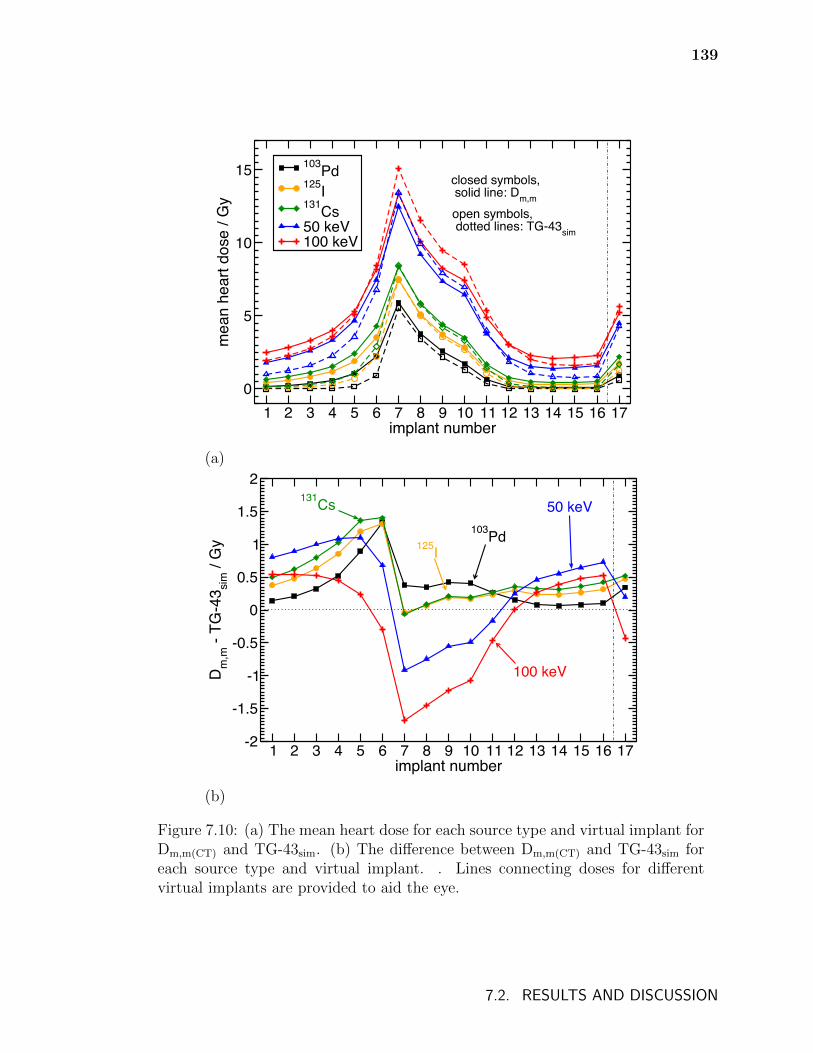
139
1 2 3 4 5 6 7 8 9 10 11 12 13 14 15 16 17implant number
0
5
10
15
mea
n he
art d
ose
/ Gy
103Pd125I131Cs50 keV100 keV
closed symbols, solid line: Dm,m
open symbols, dotted lines: TG-43sim
(a)
1 2 3 4 5 6 7 8 9 10 11 12 13 14 15 16 17implant number
-2
-1.5
-1
-0.5
0
0.5
1
1.5
2
Dm
,m -
TG-4
3 sim
/ G
y
103Pd125I
131Cs 50 keV
100 keV
(b)
Figure 7.10: (a) The mean heart dose for each source type and virtual implant forDm,m(CT) and TG-43sim. (b) The difference between Dm,m(CT) and TG-43sim foreach source type and virtual implant. . Lines connecting doses for differentvirtual implants are provided to aid the eye.
7.2. RESULTS AND DISCUSSION
140
Given this apparent relationship of heart disease to dose, the modest over-and under-
estimations in mean dose due to TG-43 calculations as well as the greater mean heart
doses for higher energy sources presented here should be taken into consideration.
7.3 Conclusions
Monte Carlo calculated doses to treatment volumes as well as to the ipsilateral lung,
heart, and aorta were calculated for a variety of virtual implants within a computa-
tional phantom derived from patient CT and organ-contour data. Doses were calcu-
lated for 103Pd, 125I, and 131Cs seeds in addition to 50 keV and 100 keV monoener-
getic point sources with full model-based calculations and TG-43-based calculations.
Considerable variation with source energy and differences between model-based and
TG-43-based doses were found for both treatment volumes and critical organs.
Differences in dose metrics to treatment volumes are due to the combined effects
of source energy, implant deformation, and the attenuation, absorption, and scattering
conditions due to the tissues in the vicinity of the implants (as discussed for 125I and
131Cs implants in chapter 6). Dose metrics for model-based calculations vary to a
greater degree between source types and between implants than for TG-43-based
calculations as model-based calculations account for tissue heterogeneity effects. The
minimum doses received by the 90% hottest volumes (D90) are generally greater for
TG-43-based calculations than for model-based dose calculations but this is not true
universally. In contrast with the results reported by Yang and Rivard55 (who found
that mean PTV doses differed by only a few percent), treatment volume dose metrics
were found to differ considerably (up to 50%) between model-based and TG-43-based
calculations. Dose metrics vary with source energy but the effect of source energy
depends on the particular metrics and treatment volumes considered.
7.3. CONCLUSIONS
141
For model-based calculations, mean doses to the ipsilateral lung decrease with
increasing source energy while for TG-43-based calculations, mean doses to the lung
increase considerably with increasing source energy. Differences between model-based
and TG-43-based calculated mean dose to the lung increase for lower energy sources,
underlining the importance of model-based dose calculations for comparing radionu-
clides in brachytherapy.
Doses to the heart and aorta generally increase with increasing source energy.
For 100 keV sources, clinically-relevant doses to the heart are calculated for even
those implants on the lateral side of the lung and these doses are underestimated
by approximately 50% by TG-43-based calculations. This has implications for the
adoption of 169Yb treatments with its mean emitted photon energy of 93 keV. TG-
43-based calculations generally underestimate the dose to the heart and aorta, in
agreement with the results of Yang and Rivard55. However, for the implants nearest
to the heart and aorta, TG-43-based calculations can overestimate the dose to these
organs due to differences in attenuation and scattering conditions between water and
patient-based phantoms.
The considerable differences in doses to treatment volumes and organs at risk
between model-based and TG-43-based calculations as well as the strong variation in
dose with source energy presented in this chapter suggest that the adoption of new
radionuclides for brachytherapy should be undertaken with caution. The results of
this chapter suggest that model-based dose calculations are crucial for the accurate
study of radiobiological effects, selection of prescription doses, and comparison of
clinical endpoints for permanent implant lung brachytherapy.
7.3. CONCLUSIONS
Chapter 8
Conclusions
8.1 Overview
Compared to external beam radiation therapy, the use of patient-specific Monte Carlo
calculations has only recently been utilized for brachytherapy. The predominant
photon interactions for the energies of low-energy permanent implant brachytherapy
cause significant differences between model-based dose calculations and the current
water-based TG-43 approach. While considerable research had been done on this
subject when the work for this thesis was initiated, many issues were still unresolved
and, in the case of permanent implant brachytherapy, completely unexplored. This
thesis studied the accurate application of Monte Carlo dose calculations to permanent
implant breast and lung brachytherapy.
Current model-based dose calculation practices for permanent implant breast
brachytherapy have previously involved the modelling of patient breasts with a single
tissue with an elemental composition that averaged adipose and fibroglandular tis-
sues. The changes in Monte Carlo calculated doses that occur with the segmentation
of breast tissues in computational phantoms were investigated. Despite significant
clinical adoption of permanent implant 125I lung brachytherapy treatments and the
highly heterogeneous nature of the lung, doses for 125I lung brachytherapy have been
142
143
calculated nearly exclusively with the water-based TG-43 formalism and no patient-
specific model-based dose calculations had ever been reported before this work. In
this thesis, the use of model-based dose calculations to determine patient-specific dose
distributions for permanent implant lung brachytherapy patients was explored: the
modelling choices for creating CT-derived patient-specific computational phantoms
that significantly affect dose distributions were discovered and differences between
model-based calculations and water-based TG-43 calculations were determined. Im-
proved techniques for generating lung brachytherapy computational phantoms were
studied by investigating various metallic artifact mitigation techniques and the use of
organ-constrained tissue assignment schemes. Finally, Monte Carlo calculations were
used to better understand the limitations of current treatment planning practices for
permanent implant lung brachytherapy and to gain a comprehensive understanding
of doses to treatment volumes and organs at risk and the variation of those doses
with source energy.
8.2 Summary of conclusions
Chapter 3 presented a study of the segmentation of breast tissues in computational
phantoms and found that the current practices at the time of using averaged tis-
sue phantoms were insufficient for accurately simulating photon energy fluence for
permanent implant breast brachytherapy. However, averaged-tissues were found to
be sufficient for calculating dose volume metrics provided that the metrics were re-
ported for gland and adipose tissues combined and that no calcifications were present.
The methods commonly used in mammography radiation protection calculations were
found to overestimate the average dose to glandular tissue.
Chapter 4 presented an initial exploration of model-based dose calculations for
8.2. SUMMARY OF CONCLUSIONS
144
125I lung brachytherapy. Patient specific Monte Carlo dose calculations for permanent
implant lung brachytherapy differed significantly from water-based TG-43 calcula-
tions and were sensitive to metallic artifact reduction techniques and tissue assign-
ment schemes. Doses were found to be insensitive to small errors in the assignment
of voxel mass density and to the padding of computational phantoms with regions of
water.
Improvements on the patient-specific Monte Carlo calculations of chapter 4 were
presented in chapter 5 which investigated the use of various metallic artifact miti-
gation techniques and organ-constrained tissue assignment for lung brachytherapy.
Of the phantom models studied, the most accurate model was determined to be a
computational phantom generated using a tissue assignment scheme that constrained
assignment within lung contours to only lung and air that was applied to CT im-
ages that received virtual sinogram metallic artifact reduction followed by simple
threshold replacement. Improved dose distributions for phantoms generated using
organ-constrained tissue assignment schemes served to reinforce the recommenda-
tions in the report of the AAPM Task Group 186 on model-based dose calculation
methods in brachytherapy beyond the TG-43 formalism. Results suggested that the
variation in the unknown composition of fibrotic tissue was not likely to significantly
affect dose distributions.
Chapter 6 used Monte Carlo methods to investigate lung brachytherapy treat-
ment planning. Calculated prescription doses were found to change significantly with
the medium in which dose was calculated. Calculating a prescription dose to two
points defined above a planar grid was found to be insufficient for reliably produc-
ing desired dose distributions in patients. The results of this chapter suggested that
any effective treatment planning practice for permanent implant lung brachytherapy
would need to account, at least approximately, for the deformation of implants in
8.2. SUMMARY OF CONCLUSIONS
145
patients and the tissues found in the vicinity of the implants.
Chapter 7 presented Monte Carlo calculated doses to treatment volumes and
organs at risk for permanent implant lung brachytherapy. Differences between model-
based and TG-43-based doses and the variation of doses with source energy were
studied. Considerable differences between model-based and TG-43-based doses were
observed for both treatment volumes and critical organs. Doses to critical organs
and treatment volumes as well as differences between model-based and TG-43-based
calculated doses varied significantly with source energy. TG-43-based calculations
generally underestimated the dose to the heart and aorta except for implants nearest
to the heart and aorta where TG-43-based calculations overestimated the dose to these
organs due to differences in attenuation and scattering conditions between water- and
patient-based phantoms. These results underline the importance of using model-based
dose calculation algorithms to achieve accurate dose calculations of permanent lung
implant brachytherapy and that MBDCAs must play a crucial role in future study of
radiobiological effects, the selection of prescription doses, and in the comparison of
clinical endpoints for these treatments.
8.3 Impact and future work
This thesis represents a contribution towards the accurate application of patient spe-
cific Monte Carlo calculations for permeant implant breast and lung brachytherapy
and for low-energy brachytherapy in general. The use of tissue segmentation in
brachytherapy, which had previously been largely ignored, was shown to significantly
affect dose distributions. The comparison of metallic artifact methods in chapters
4 and 5 and the calculation of resulting dose distributions from artifact corrected
phantoms as well as the comparison of unconstrained and organ-constrained tissue
8.3. IMPACT AND FUTURE WORK
146
assignments for brachytherapy represent novel contributions to the field of model-
based dose calculations. Additionally, this work presented insights into the treatment
planning, doses to treatment volumes and organs at risk, and the variation in doses
with radionuclides for permanent implant lung brachytherapy which, to date, had
been informed entirely by water-based TG-43 calculations. Despite these contribu-
tions, continuation of the work of this thesis as well as improvements in the application
of model-based dose calculations to low-energy brachytherapy in general are required
before these methods can be adopted clinically.
The model-based dose calculation techniques for lung brachytherapy patients
described in chapters 4 and 5 would likely require experimental validation before
clinical adoption. This could be achieved by creating a physical phantom of a realistic
human chest containing a removable lung brachytherapy implant. By acquiring CT
images of the phantom with and without brachytherapy seeds, the performance of the
metallic artifact reduction methods could be tested by comparing dose distributions
generated from explicitly defined and CT-derived phantom models. Additionally,
given prior knowledge of the elemental composition of the phantom structures, tissue
assignment schemes which convert CT number to elemental compositions could be
validated.
The work presented in this thesis illustrated the strong sensitivity of dose distri-
butions to voxel elemental compositions for low-energy brachytherapy. Confirmation
of the elemental compositions of human tissues, which have been reported by only a
few studies in the past 30 years, as well as a comprehensive study of the variation
of tissue compositions between people is necessary to reach sufficient confidence in
patient-specific Monte Carlo dose calculations of low-energy brachytherapy for clinical
adoption.
8.3. IMPACT AND FUTURE WORK
References
[1] Canadian Cancer Society, Canadian Cancer Statistics 2013, Technical report,Canadian Cancer Society, Toronto, Canada, 2013. (page 1)
[2] Canadian Cancer Society, Radiation Therapy: A guide for people with can-cer 2013, Technical report, Canadian Cancer Society, Toronto, Canada, 2013.(page 1)
[3] National Cancer Institute, Radiation therapy for cancer, 2013. (page 1)
[4] E. B. Podgorsak, editor, Radiation Oncology Physics: A Handbook for Teachersand Students, Educational Report Series, IAEA, Vienna, Austria, 2005. (page 2)
[5] B. S. Hilaris, U. K. Henschke, and J. G. Holt, Clinical experience with longhalf-life and low-energy encapsulated radioactive sources in cancer radiationtherapy, Radiology 91, 1163–1167 (1968). (page 2)
[6] J.-P. Pignol, B. Keller, E. Rakovitch, R. Sankreacha, H. Easton, and W. Que,First report of a permanent breast 103Pd seed implant as adjuvant radiationtreatment for early-stage breast cancer, Int. J. Radiat. Oncol. Biol. Phys. 64,176 – 181 (2006). (pages 2, 3)
[7] B. Keller, R. Sankreacha, E. Rakovitch, P. O’Brien, and J.-P. Pignol, A per-manent breast seed implant as partial breast radiation therapy for early-stagepatients: A comparison of palladium-103 and iodine-125 isotopes based on ra-diation safety considerations, Int. J. Radiat. Oncol. Biol. Phys. 62, 358 – 365(2005). (page 2)
[8] T. A. d’Amato, M. Galloway, G. Szydlowski, A. Chen, and R. J. Landreneau,Intraoperative brachytherapy following thoracoscopic wedge resection of stageI lung cancer, Chest 114, 1112 – 1115 (1998). (pages 2, 4)
[9] A. Chen, M. Gallowy, R. Landreneau, T. d’Amato, A. Colonias, S. Karlovits,A. Quinn, T. Santucci, S. Kalnicki, and D. Brown, Intraoperative 125Ibrachytherapy for high-risk stage I non-small cell lung carcinoma, Int. J. Radiat.Oncol. Biol. Phys. 44, 1057 – 1063 (1999). (pages 2, 4, 43, 95)
[10] T. Whelan, R. MacKenzie, J. Julian, M. Levine, W. Shelly, L. Grimard, B. Lada,H. Lukka, F. Perera, and A. F. et.al., Randomized trial of breast irradiationschedules after lumpectomy for women with lymph node-negative breast cancer,Journal of the National Cancer Institute 94, 1143–1150 (2002). (page 3)
147
148
[11] Canadian Cancer Society, Canadian Cancer Statistics 2011, Technical report,Canadian Cancer Society, Toronto, Canada, 2011. (page 4)
[12] American Cancer Society, Cancer Facts and Figures, Technical report, Ameri-can Cancer Society, 2011. (page 4)
[13] R. Rami-Porta and M. Tsuboi, Sublobar resection for lung cancer, EuropeanRespiratory Journal 33, 426 – 435 (2009). (page 4)
[14] W. H. Warren and L. P. Faber, Segmentectomy versus lobectomy in patientswith stage I pulmonary carcinoma: five year survival and patterns of intratho-racic recurrence, J. Thorac. Cardiovasc. Surg. 107, 1087–1094 (1994). (page 4)
[15] M. Johnson, A. Colonias, D. Parda, M. Trombetta, O. Gayou, B. Reitz, andM. Miften, Dosimetric and technical aspects of intraoperative I-125 brachyther-apy for stage I non-small cell lung cancer, Phys. Med. Biol. 52, 1237 – 1245(2007). (pages 4, 95, 98, 123)
[16] W. Lee, B. D. T. Daly, T. A. DiPetrillo, D. M. Morelli, A. C. Neuschatz,J. Morr, and M. J. Rivard, Limited resection for non-small cell lung cancer:Observed local control with implantation of I-125 brachytherapy seeds, Ann.Thorac. Surg. 75, 237 – 243 (2003). (page 4)
[17] R. Santos, A. Colonias, D. Parda, M. Trombetta, R. H. Maley, R. Macherey,S. Bartley, T. Santucci, R. J. Keenan, and R. J. Landreneau, Comparisonbetween sublobar resection and 125Iodine brachytherapy after sublobar resectionin high-risk patients with Stage I non-small-cell lung cancer, Surgery 134, 691– 697 (2003). (pages 4, 118)
[18] G. Voynov, D. E. Heron, C. J. Lin, S. Burton, A. Chen, A. Quinn, R. Santos,A. Colonias, and R. J. Landreneau, Intraoperative 125I Vicryl mesh brachyther-apy after sublobar resection for high-risk stage I nonsmall cell lung cancer,Brachytherapy 4, 278 – 285 (2005). (page 4)
[19] A. J. Stewart, S. Mutyala, C. L. Holloway, Y. L. Colson, and P. M. Devlin,Intraoperative seed placement for thoracic malignancy – A review of technique,indictations, and published literature, Brachytherapy 8, 63 – 69 (2009). (page 4)
[20] S. Mutyala, A. Steward, A. J. Khan, R. A. Cormack, D. O’Farrell, D. Sug-arbaker, and P. M. Devlin, Permanent iodine-125 interstitial planar seedbrachytherapy for close or positive margins for thoracic malignancies, Int. J.Radiat. Oncol. Biol. Phys. 76, 1114 – 1120 (2010). (page 4)
[21] B. Parashar, A. G. Wernicke, A. Pavese, P. Singh, S. Trichter, A. Sabbas, D. I.Kutler, W. Kuhel, J. L. Port, P. C. Lee, D. Nori, and K. S. C. Chao, Cesium-131permanent seed brachytherapy: Dosimetric evaluation and radiation exposureto surgeons, radiation oncologists, and staff, Brachytherapy 10, 508 –513 (2011).(pages 4, 95, 117, 118)
REFERENCES
149
[22] K. L. Leonard and T. A. DiPetrillo and J. J. Munro and D. E. Wazer, A novelytterbium-169 brachytherapy source and delivery system for use in conjunctionwith minimally invasive wedge resection of early-stage lung cancer, Brachyther-apy 10, 163 – 169 (2011). (pages 4, 117)
[23] H. C. Fernando, R. J. Landreneau, S. J. Mandrekar, S. L. Hillman, F. C. Nichols,B. Meyers, T. A. DiPetrillo, D. Heron, D. R. Jones, and B. D. T. Daly, The im-pact of adjuvant brachytherapy with sublobar resection on pulmonary functionand dyspnea in high-risk patients with operable disease: preliminary resultsfrom the American College of Surgeons Oncology Group Z4032 trial, The Jour-nal of thoracic and cardiovascular surgery 142, 554–562 (2011). (page 4)
[24] M. J. Rivard, J. L. M. Venselaar, and L. Beaulieu, The evolution of brachyther-apy treatment planning, Med. Phys. 36, 2136 – 2153 (2009). (pages 5, 7, 8,43)
[25] R. Nath, L. L. Anderson, G. Luxton, K. A. Weaver, J. F. Williamson, and A. S.Meigooni, Dosimetry of interstitial brachytherapy sources: Recommendationsof the AAPM Radiation Therapy Committee Task Group No. 43, Med. Phys.22, 209 – 234 (1995). (pages 5, 43, 95)
[26] M. J. Rivard, B. M. Coursey, L. A. DeWerd, M. S. Huq, G. S. Ibbott, M. G.Mitch, R. Nath, and J. F. Williamson, Update of AAPM Task Group No. 43Report: A revised AAPM protocol for brachytherapy dose calculations, Med.Phys. 31, 633 – 674 (2004). (pages 5, 6, 7, 19, 43, 95, 97)
[27] M. J. Rivard, W. M. Butler, L. A. DeWerd, M. S. Huq, G. S. Ibbott, A. S. Mei-gooni, C. S. Melhus, M. G. Mitch, R. Nath, and J. F. Williamson, Supplementto the 2004 update of the AAPM Task Group No. 43 Report, Med. Phys. 34,2187 – 2205 (2007). (pages 5, 43, 95, 99)
[28] N. Papanikolaou, J. J. Battista, A. L. Boyer, C. Kappas, E. Klein, T. R. Mackie,M. Sharpe, and J. van Dyk, Tissue inhomogeneity corrections for megavoltagephoton beams, AAPM Report 85, Medical Physics Pub for AAPM, New York,2004. (page 8)
[29] L. Beaulieu, A. C. Tedgren, J.-F. Carrier, S. D. Davis, F. Mourtada, M. J.Rivard, R. M. Thomson, F. Verhaegen, T. A. Wareing, and J. F. Williamson,Report of the Task Group 186 on model-based dose calculation methods inbrachytherapy beyond the TG-43 formalism: Current status and recommenda-tions for clinical implementation, Med. Phys. 39, 6208 – 6236 (2012). (pages 8,73, 94)
[30] M. J. Berger and J. H. Hubbell, XCOM: Photon cross sections on a personalcomputer, Report NBSIR87–3597, National Institute of Standards Technology(NIST), Gaithersburg, MD 20899, U.S.A., 1987. (pages 9, 16, 21, 51, 97, 120)
[31] P. Mobit and I. Badragan, Dose perturbation effects in prostate seed implantbrachytherapy with I-125, Phys. Med. Biol. 49, 3171 – 3178 (2004). (page 9)
REFERENCES
150
[32] B. Reniers, F. Verhaegen, and S. Vynckier, The radial dose function of low-energy brachytherapy seeds in different solid phantoms: comparison betweencalculations with the EGSnrc and MCNP4C Monte Carlo codes and measure-ments, Phys. Med. Biol. 49, 1569 – 1582 (2004). (page 9)
[33] O. Chibani, J. F. Williamson, and D. Todor, Dosimetric effects of seedanisotropy and interseed attenuation for 103Pd and 125I prostate implants, Med.Phys. 32, 2557 – 2566 (2005). (pages 9, 10)
[34] J.-F. Carrier, L. Beaulieu, F. Therriault-Proulx, and R. Roy, Impact of interseedattenuation and tissue composition for permanent prostate implants, Med.Phys. 33, 595 – 604 (2006). (pages 9, 10)
[35] H. Afsharpour, M. D’Amours, B. Cote, J.-F. Carrier, F. Verhaegen, andL. Beaulieu, A Monte Carlo study on the effect of seed design on the inter-seed attenuation in permanent prostate implants, Med. Phys. 35, 3671 – 3681(2008). (pages 9, 10)
[36] R. E. Taylor, Monte Carlo Calculations for Brachytherapy, MSc Thesis, Car-leton University, Ottawa, Ontario (2006). (page 9)
[37] J.-F. Carrier, M. D’Amours, F. Verhaegen, B. Reniers, A.-G. Martin, E. Vi-gneault, and L. Beaulieu, Postimplant dosimetry using a Monte Carlo dosecalculation engine: a new clinical standard, Int. J. Radiat. Oncol. Biol. Phys.68, 1190 – 1198 (2007). (pages 9, 10)
[38] C. S. Melhus and M. J. Rivard, COMS eye plaque brachytherapy dosimetrysimulations for 103Pd, 125I, and 131Cs, Med. Phys. 35, 3364 – 3371 (2008).(pages 9, 10)
[39] R. M. Thomson, R. E. P. Taylor, and D. W. O. Rogers, Monte Carlo dosimetryfor 125I and 103Pd eye plaque brachytherapy, Med. Phys. 35, 5530 – 5543 (2008).(pages 9, 10)
[40] C. Furstoss et al, Monte Carlo study of LDR seed dosimetry with an applicationin a clinical brachytherapy breast implant, Med. Phys. 36, 1848 – 1858 (2009).(pages 9, 10, 22)
[41] H. Afsharpour, J.-P. Pignol, B. Keller, J.-F. Carrier, B. Reniers, F. Verhaegen,and L. Beaulieu, Influence of breast composition and interseed attenuation indose calculations for post-implant assessment of permanent breast 103Pd seedimplant, Phys. Med. Biol. 55, 4547 – 4561 (2010). (pages 9, 10, 22)
[42] G. Landry, B. Reniers, L. Murrer, L. Lutgens, E. Bloemen-Van Gurp, J.-P.Pignol, B. Keller, L. Beaulieu, and F. Verhaegen, Sensitivity of low energybrachytherapy Monte Carlo dose calculations to uncertainties in human tissuecomposition., Med. Phys. 37, 5188 – 5198 (2010). (pages 9, 10, 102)
[43] S. H. Cho, O. N. Vassiliev, S. Lee, H. H. Liu, G. S. Ibbott, and R. Mohan,Reference photon dosimetry data and reference phase space data for the 6 MV
REFERENCES
151
photon beam from Varian Clinac 2100 series linear accelerators, Med. Phys.32, 137 – 148 (2005). (page 10)
[44] W. Schneider, T. Bortfeld, and W. Schlegel, Correlation between CT numbersand tissue parameters needed for Monte Carlo simulations of clinical dose dis-tributions, Phys. Med. Biol. 45, 459 – 478 (2000). (pages 10, 18, 44, 50, 72,77)
[45] J. V. Siebers, P. J. Keall, A. E. Nahum, and R. Mohan, Converting absorbeddose to medium to absorbed dose to water for Monte Carlo based photon beamdose calculation, Phys. Med. Biol. 45, 983 – 995 (2000). (pages 10, 18, 50, 77)
[46] H. Jiang and J. Seco and H. Paganetti, Effects of Hounsfield number conversionon CT based proton Monte Carlo dose calculations, Med. Phys. 34, 1439 – 1449(2007). (page 10)
[47] H. Paganetti, Dose to water versus dose to medium in proton beam therapy,Phys. Med. Biol. 54, 4399 – 4421 (2009). (pages 10, 50, 77)
[48] F. Verhaegen and S. Devic, Sensitivity study for CT image use in Monte Carlotreatment planning, Phys. Med. Biol. 50, 937 – 946 (2005). (pages 10, 18, 102)
[49] M. Bazalova, L. Beaulieu, S. Palefsky, and V. Verghaegen, Correction of CTartifacts and its influence on Monte Carlo dose calculations, Med. Phys. 34,2119 – 2132 (2007). (pages 10, 46)
[50] C. Xu, F. Vergaegen, D. Laurendeau, S. A. Enger, and L. Beaulieu, An algo-rithm for efficient metal artifact reductions in permanent seed implants, Med.Phys. 38, 47 – 56 (2011). (pages 10, 44, 68)
[51] Y. Takahashi, S. Mori, T. Kozuka, K. Gomi, T. Nose, T. Tahara, M. Oguchi, andT. Yamashita, Preliminary study of correction of metal artifacts due to I-125seeds in postimplant dosimetry for prostate permanent implant brachytherapy,Radiat. Med. 24, 133 – 138 (2006). (pages 10, 44)
[52] P. S. Basran, A. Robertson, and D. Wells, CT image artifacts from brachyther-apy seed implants: A postprocessing 3D adaptive median filter, Med. Phys. 38,712 – 718 (2011). (pages 10, 44, 68, 72, 74, 81)
[53] H. Afsharpour, G. Landry, B. Reniers, J. P. Pignol, L. Beaulieu, and F. Ver-haegen, Tissue modeling schemes in low energy breast brachytherapy, Phys.Med. Biol. 56, 7045 – 7060 (2011). (page 10)
[54] M. J. Rivard et.al., Comparison of dose calculation methods for brachytherapyof intraocular tumors, Med. Phys. 38, 306 – 316 (2011). (page 10)
[55] Y. Yang and M. J. Rivard, Evaluation of brachytherapy lung implant dosedistributions from photon-emitting sources due to tissue heterogeneities, Med.Phys. 38, 5857 – 5862 (2011). (pages 10, 43, 117, 140, 141)
REFERENCES
152
[56] I. Kawrakow and D. W. O. Rogers, The EGSnrc Code System: Monte Carlosimulation of electron and photon transport, Technical Report PIRS–701, Na-tional Research Council of Canada, Ottawa, Canada, 2000. (page 13)
[57] I. Kawrakow, Accurate condensed history Monte Carlo simulation of electrontransport. I. EGSnrc, the new EGS4 version, Med. Phys. 27, 485 – 498 (2000).(page 13)
[58] W. R. Nelson, H. Hirayama, and D. W. O. Rogers, The EGS4 code system,Report SLAC–265, Stanford Linear Accelerator Center, Stanford, California,1985. (page 13)
[59] F. H. Attix, Introduction to Radiological Physics and Radiation Dosimetry,Wiley, New York, 1986. (page 13)
[60] E. B. Podgorsak, Radiation physics for medical physicists, Springer, Berlin,Heidelberg, New York, 2005. (page 13)
[61] H. E. Johns and J. R. Cunningham, The physics of radiology, 4th ed., CharlesC. Thomas, Springfield, Illinois, 1983. (page 13)
[62] M. J. Berger, J. H. Hubbell, S. M. Seltzer, J. Chang, J. S. Coursey, R. Sukumar,D. S. Zucker, and K. Olsen, XCOM: Photon cross section database (version1.5), Technical report, NIST, Gaithersburg, MD, http://physics.nist.gov/xcom,2010. (page 13)
[63] M. J. Berger, Monte Carlo Calculation of the penetration and diffusion of fastcharged particles, in Methods in Comput. Phys., edited by B. Alder, S. Fernbach,and M. Rotenberg, volume 1, pages 135 – 215, Academic, New York, 1963.(page 13)
[64] I. Kawrakow and A. F. Bielajew, On the condensed history technique forelectron transport, Nuclear Instruments and Methods 142B, 253 – 280 (1998).(page 13)
[65] I. Kawrakow, Electron impact ionization cross sections for EGSnrc, Med. Phys.(abstract) 29, 1230 (2002). (page 14)
[66] R. E. P. Taylor, G. Yegin, and D. W. O. Rogers, Benchmarking BrachyDose:voxel-based EGSnrc Monte Carlo calculations of TG–43 dosimetry parameters,Med. Phys. 34, 445 – 457 (2007). (pages 14, 15, 16, 21)
[67] R. M. Thomson, G. Yegin, R. E. P. Taylor, J. G. H. Sutherland, and D. W. O.Rogers, Fast Monte Carlo dose calculations for brachytherapy with BrachyDose,Med. Phys. 37, (abstract) 3910 – 3911 (2010). (page 14)
[68] C. Thomason, T. Mackie, M. Lindstrom, and P. Higgins, The dose distributionsurrounding Ir-192 and Cs-137 seed sources, Phys. Med. Biol. 36, 475 – 493(1991). (page 14)
REFERENCES
153
[69] G. Luxton, Comparison of radiation-dosimetry in water and in solid phantommaterials for I-125 and Pd-103 brachytherapy sources - EGS4 Monte Carlostudy, Med. Phys. 21, 621 – 641 (1994). (page 14)
[70] R. Wang and R. S. Sloboda, EGS4 dosimetry calculations for cylindricallysymmetric brachytherapy sources, Med. Phys. 23, 1459 – 1465 (1996). (page 14)
[71] E. Mainegra, R. Capote, and E. Lopez, Dose rate constants for 103Pd, 125I,196Yb, 192Ir, brachytherapy sources: an EGS4 Monte Carlo Study, Phys. Med.Biol. 43, 1557 – 1566 (1998). (page 14)
[72] G. Luxton and G. Jozsef, Radial dose distribution, dose to water and dose rateconstant for monoenergetic photon point sources from 10 keV to 2 MeV: EGS4Monte Carlo model calculation, Med. Phys. 26, 2531 – 2538 (1999). (page 14)
[73] E. Mainegra, R. Capote, and E. Lopez, Radial dose functions for 103Pd, 125I,196Yb, 192Ir, brachytherapy sources: an EGS4 Monte Carlo Study, Phys. Med.Biol. 45, 703 – 717 (2000). (page 14)
[74] R. E. Wallace, Empirical dosimetric characterization of model I125-SL 125Iodinebrachytherapy source in phantom, Med. Phys. 27, 2796 – 2802 (2000). (page 14)
[75] R. Capote, E. Mainegra, and E. Lopez, Anisotropy functions for low energyinterstitial brachytherapy sources: an EGS4 Monte Carlo Study, Phys. Med.Biol. 46, 135 – 150 (2001). (page 14)
[76] G. Yegin, A new approach to geometry modelling of Monte Carlo particletransport: an application to EGS, Nucl. Inst. Meth. B 211, 331 – 338 (2003).(pages 14, 15)
[77] R. E. P. Taylor and D. W. O. Rogers, An EGSnrc Monte Carlo-calculateddatabase of TG-43 parameters, Med. Phys. 35, 4228 – 4241 (2008). (pages 15,21, 23, 45, 98)
[78] R. E. P. Taylor and D. W. O. Rogers, EGSnrc Monte Carlo calculated dosimetryparameters for 192Ir and 169Yb brachytherapy sources, Med. Phys. 35, 4933 –4944 (2008). (page 15)
[79] M. Rodriguez and D. W. O. Rogers, On determining dose rate constantsspectroscopically, Med. Phys. 40, 011713 (10pp) (2013). (page 15)
[80] J. H. Hubbell, Photon Mass Attenuation and Energy-absorption Coefficientsfrom 1 keV to 20 MeV, Int. J. Appl. Radiat. Isot. 33, 1269 – 1290 (1982).(page 16)
[81] R. P. Parker, P. A. Hobday, and K. J. Cassell, The direct use of CT numbersin radiotherapy dosage calculations for inhomogeneous media, Phys. Med. Biol.24, 802 – 809 (1979). (page 18)
[82] I. Kawrakow, M. Fippel, and K. Friedrich, 3D Electron Dose Calculation usinga Voxel based Monte Carlo Algorithm (VMC), Med. Phys. 23, 445 – 457 (1996).(page 18)
REFERENCES
154
[83] R. T. Mull, Mass estimates by computed tomography: physical density fromCT numbers, American journal of roentgenology 143, 1101 – 1104 (1984).(page 18)
[84] D. Liu, M. Ajlouni, J. Jin, S. Ryu, F. Siddiqui, A. Patel, B. Movsas, and I. J.Chetty, Analysis of outcomes in radiation oncology: An integrated computa-tional platform, Med. Phys. 36, 1680–1689 (2009). (page 18)
[85] H. Q. Woodard and D. R. White, The composition of body tissues, Brit. J.Radiol. 59, 1209 – 1219 (1986). (pages 18, 19, 24, 50, 75, 97, 119)
[86] D. R. White, H. Q. Woodard, and S. M. Hammond, Average soft-tissue andbone models for use in radiation dosimetry, Brit. J. Radiol. 60, 907 – 913(1987). (pages 18, 19, 50)
[87] ICRU, Photon, Electron, Photon and Neutron Interaction Data for Body Tis-sues, ICRU Report 46, ICRU, Washington D.C., 1992. (pages 18, 19, 24, 50)
[88] National Electrical Manufacturers Association, DICOM: Digital Imaging andCommunications in Medicine, 2013. (page 18)
[89] M. J. Yaffe and J. M. Boone et al., The myth of the 50-50 breast, Med. Phys.36, 5437 – 5443 (2009). (pages 22, 23, 24, 25, 40)
[90] G. R. Hammerstein, D. W. Miller, D. R. White, M. E. Masterson, H. Q.Woodard, and J. S. Laughlin, Absorbed Radiation Dose in Mammography,Radiology 130, 485 – 491 (1979). (pages 22, 23, 25, 37)
[91] D. R. Dance, The Monte Carlo calculation of integral radiation dose in xero-mammogrpahy, Phys. Med. Biol. 25, 25–37 (1980). (pages 22, 23, 25)
[92] I. Sechopoulos, A. Karellas, S. Suryanarayanan, S. Vedantham, and C. D’Orsi,Computation of the glandular radiation dose in digital tomosynthesis of thebreast, Med. Phys. 34, 221 – 232 (2007). (pages 22, 23)
[93] R. C. Chen, R. Longo, L. Rigon, F. Zanconati, A. D. Pellegrin, F. Arfelli,D. Dreossi, R.-H. Menk, E. Vallazza, T. Q. Xiao, and E. Castelli, Measurementof the linear attenuation coefficients of breast tissues by synchrotron radiationcomputed tomography, Phys. Med. Biol. 55, 4993 – 5005 (2010). (page 22)
[94] P. C. Johns and M. J. Yaffe, X-ray characterisation of normal and neoplasticbreast tissues, Phys. Med. Biol. 32, 675 – 696 (1987). (page 22)
[95] G. Landry et.al., Sensitivity of low energy brachytherapy Monte Carlo dosecalculations to uncertainties in human tissue composition., Med. Phys. 37,5188 – 5198 (2010). (page 22)
[96] H. Afsharpour, J.-P. Pignol, B. Keller, J.-F. Carrier, B. Reniers, F. Ver-haegen, and L. Beaulieu, Toward a more accurate dose calculationtechnique using a semiautomatic organ contouring in Monte Carlo post-implant assessment of breast LDR brachytherapy, Abstract book of
REFERENCES
155
MCTP2009: Second European Workshop on Monte Carlo TreatmentPlanning, available at http://www.mctp2009.org/images/documents/EGW-MCTP%20Workshop%202009%20Book%20of%20Abstracts.pdf , 98 – 101(2009). (pages 22, 30)
[97] M. Bazalova and E. E. Graves, The importance of tissue segmentation fordose calculations for kilovoltage radiation therapy, Med. Phys. 38, 3039 – 3049(2011). (page 22)
[98] R. M. Thomson and D. W. O. Rogers, Monte Carlo dosimetry for 125I and103Pd eye plaque brachytherapy with various seed models, Med. Phys. 37, 368– 376 (2010). (page 23)
[99] J.-P. Pignol, E. Rakovitch, B. M. Keller, R. Sankreacha, and C. Chartier, Tol-erance and Acceptance Results of a Palladium-103 Permanent Breast Seed Im-plant Phase I/II Study, Int. J. Radiat. Oncol. Biol. Phys. 73, 1482 – 1488(2009). (page 24)
[100] E. Zastrow, S. K. Davis, M. Lazebnik, F. Kelcz, B. D. V. Veen, and S. C.Hagness, Development of Anatomically Realistic Numerical Breast PhantomsWith Accurate Dielectric Properties for Modeling Microwave Interactions Withthe Human Breast, IEEE Transactions on Biomedical Engineering 55, 2792 –2800 (2010). (pages 27, 36)
[101] O. Hassler, Microradiographic investigations of calcifications of the femalebreast, Cancer 23, 1103–1109 (1969). (page 28)
[102] D. M. Hansell, J. C. Cooke, C. A. Parsons, S. H. Evans, D. R. Dance, J. M.Bliss, and I. Ilesley, A quantitative analysis of the spatial relationships ofgrouped microcalcifications demonstrated on xeromammography in benign andmalignant breast disease, Brit. J. Radiol. 61, 21–25 (1988). (page 28)
[103] M. Abdoli, M. R. Ay, A. Ahmadian, and H. Zaidi, A virtual sinogram methodto reduce dental metallic implant artefacts in computed tomography-based at-tenuation correction for PET, Nuclear Medicine Communications 31, 22 – 31(2010). (page 46)
[104] M. Abdoli, M. R. Ay, A. Ahmadian, R. A. J. O. Dierckx, and H. Zaidi, Re-duction of dental filling metallic artifacts in CT-based attenuation correction ofPET data using weighted virtual sinograms optimized by a genetic algorithm,Med. Phys. 37, 6166 – 6177 (2010). (page 46)
[105] W. A. Kalender, R. Hebel, and J. Ebersberger, Reduction of CT artifactscaused by metallic implants, Radiology 164, 576 – 577 (1987). (page 46)
[106] J. C. Roeske, C. Lund, C. A. Pelizzari, X. Pan, and A. J. Mundt, Reductionof computed tomography metal artifacts due to the Fletcher-Suit applicator ingynecology patients receiving intracavitary brachytherapy, Brachytherapy 2,207 – 214 (2003). (page 46)
REFERENCES
156
[107] M. Yazdi, L. Gingras, and L. Beaulieu, An adaptive approach to metal arti-fact reduction in helical computed tomography for radiation therapy treatmentplanning: Experimental and clinical studies, Int. J. Radiat. Oncol. Biol. Phys.62, 1224 – 1231 (2005). (page 46)
[108] G. Landry, P. V. Granton, B. Reniers, M. C. Ollers, L. Beaulieu, J. E. Wilderger,and F. Vergaegen, Simulation study on potential accuracy gains from dualenergy CT tissue segmentation for low-energy brachytherapy Monte Carlo dosecalculations, Phys. Med. Biol. 56, 6257 – 6278 (2011). (pages 69, 102)
[109] K. M. Furutani, R. C. Miller, L. B. McLemore, C. C. Goulet, D. H. Brinkmann,and M. G. Haddock, 4D CT dosimetric analysis of the Mayo Clinic brachyther-apy technique for a cholangiocarcinoma patient, Brachytherapy 5, 84 (2006).(page 70)
[110] R. O. Ottosson and C. F. Behrens, CTC-ask: a new algorithm for conversionof CT numbers to tissue parameters for Monte Carlo dose calculations applyingDICOM RS knowledge, Phys. Med. Biol. 56, N263–N274 (2011). (page 73)
[111] J. G. H. Sutherland, K. M. Furutani, Y. I. Garces, and R. M. Thomson, Model-based dose calculations for 125I lung brachytherapy, Med. Phys. 39, 4365 –4377(2012). (pages 89, 93, 100)
[112] M. J. Rivard, Brachytherapy dosimetry parameters calculated for a 131Cssource, Med. Phys. 34, 754 – 762 (2007). (page 97)
[113] Brookhaven National Laboratory, National Nuclear Data Center,http://www.nndc.bnl.gov/nudat2. (page 97)
[114] S. Thomas, A. Colonias, H. Odau, R. K. Das, S. M. Bentzen, R. R. Patel,and D. Khuntia, Feasibility of Cs-131 for intraoperative brachytherapy for pa-tients undergoing sublobar resections for early stage non-small cell lung cancer(NSCLC): A dosimetric comparison with I-125 and Cs-131, Brachytherapy 106,108 (2007). (page 117)
[115] D. Nori, X. Li, and T. Pugkhem, Intraoperative brachytherapy using gelfoamradioactive plaque implants for resected stage III non-small cell lung cancerwith positive margin: A pilot study, Journal of surgical oncology 60, 257–261(1995). (page 117)
[116] S. A. Enger, D. R. Fisher, and R. T. Flynn, Gadolinium-153 as a brachytherapyisotope, Phys. Med. Biol. 58, 957 – 964 (2013). (page 117)
[117] M. G. Trombetta, A. Colonias, D. Makishi, R. Keenan, E. D. Werts, R. Landre-neau, and D. S. Parda, Tolerance of the aorta using intraoperative iodine-125interstitial brachytherapy in cancer of the lung, Brachytherapy 7, 50 – 54(2008). (pages 118, 136)
[118] L. B. Marks et al, Radiation dose-volume effects in the lung, Int. J. Radiat.Oncol. Biol. Phys. 76, S70 – S76 (2010). (page 134)
REFERENCES
157
[119] J. L. W. S. A. Mccormick, B. Sood, A. Alieri, and B. Vikram, Tolerance ofthe carotid sheath contents to brachytherapy: An experimental study, TheLaryngoscope 101, 587 – 591 (1991). (page 136)
[120] S. C. Darby et al., Radiation-related heart disease: current knowledge andfuture prospects, Int. J. Radiat. Oncol. Biol. Phys. 76 (2010). (page 138)
[121] S. C. Darby et al., Risk of Ischemic Heart Disease in Women after Radiotherapyfor Breast Cancer, New England Journal of Medicine 368, 987–998 (2013).(page 138)
REFERENCES