Haik Kalantarian

Arthur Matsumoto

Monte Carlo Analysis

Why Quasi-Monte Carlo is Better Than Monte Carlo or Latin

Hypercube Sampling for Statistical Circuit Analysis

Singhee, A.; Rutenbar, R.A.; , "Why Quasi-Monte Carlo is Better Than

Monte Carlo or Latin Hypercube Sampling for Statistical Circuit

Analysis," Computer-Aided Design of Integrated Circuits and Systems, IEEE

Transactions on , vol.29, no.11, pp.1763-1776, Nov. 2010

doi: 10.1109/TCAD.2010.2062750

URL:

http://ieeexplore.ieee.org/stamp/stamp.jsp?tp=&arnumber=5605333

&isnumber=5605300

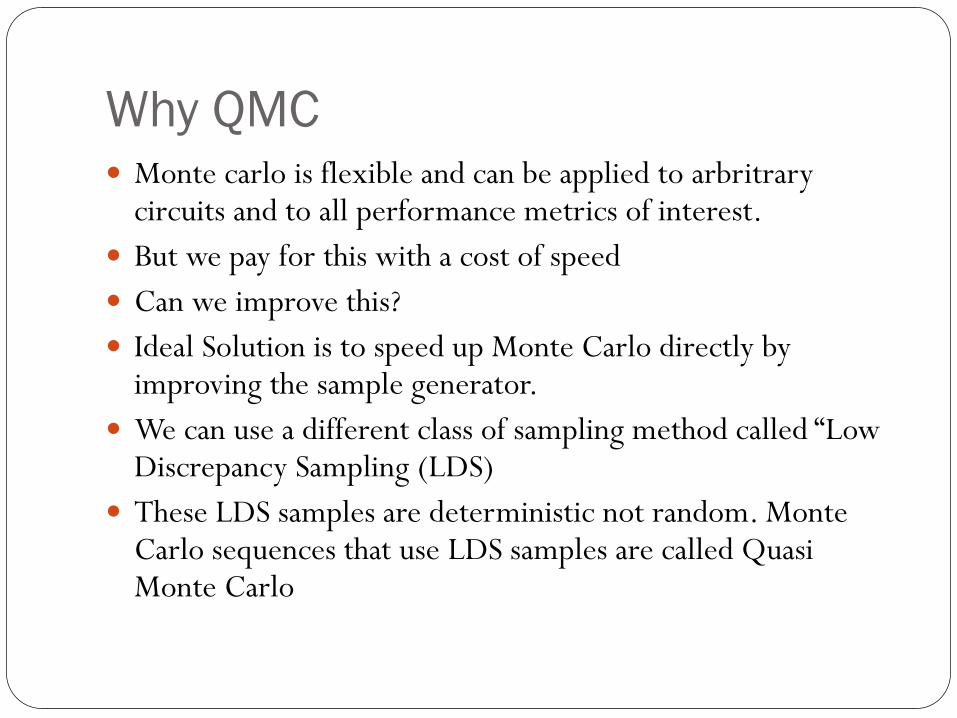
Why QMC Monte carlo is flexible and can be applied to arbritrary

circuits and to all performance metrics of interest.

But we pay for this with a cost of speed

Can we improve this?

Ideal Solution is to speed up Monte Carlo directly by improving the sample generator.

We can use a different class of sampling method called “Low Discrepancy Sampling (LDS)

These LDS samples are deterministic not random. Monte Carlo sequences that use LDS samples are called Quasi Monte Carlo

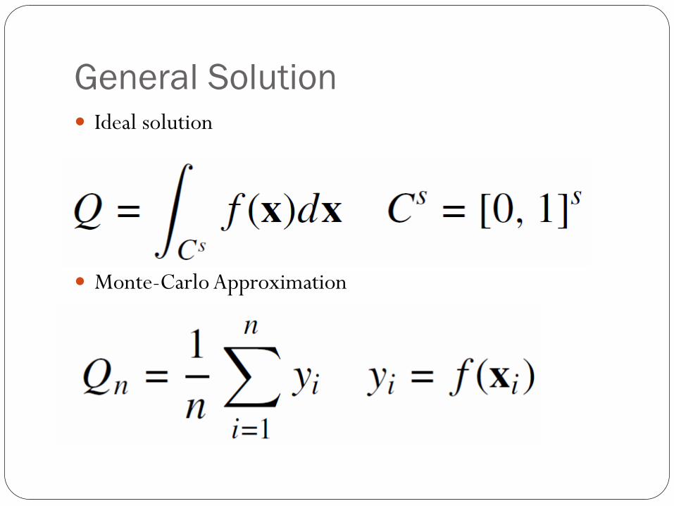
General Solution Ideal solution

Monte-Carlo Approximation

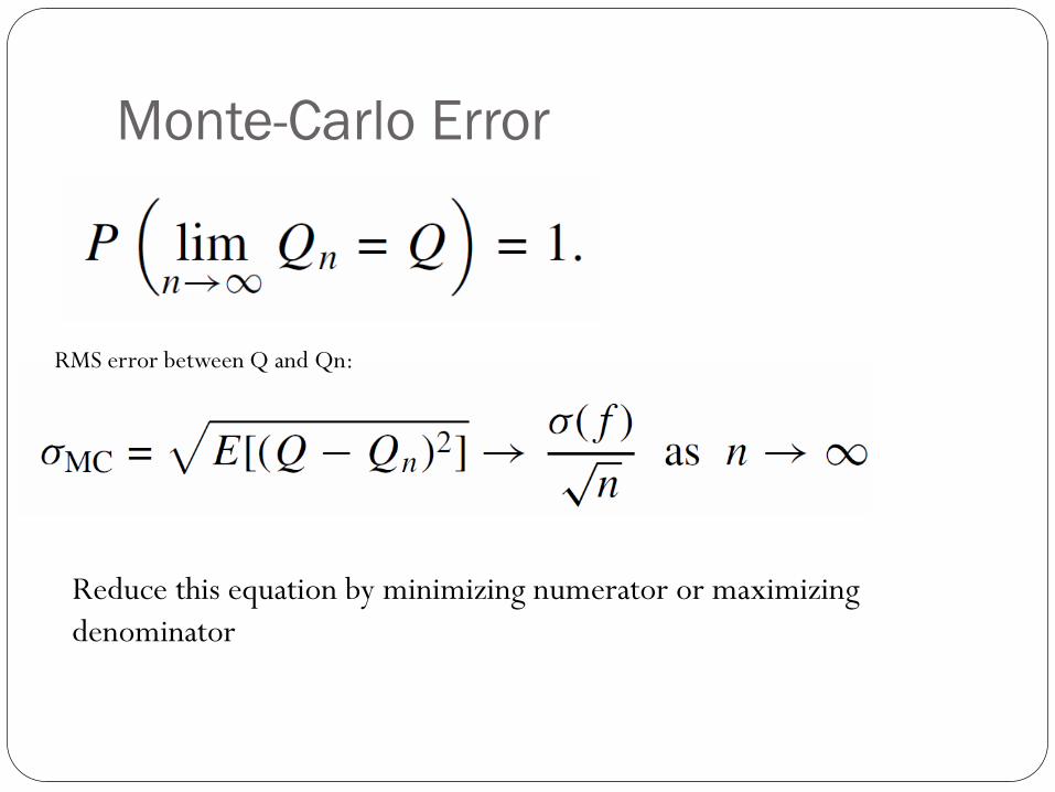
Monte-Carlo Error

RMS error between Q and Qn:

Reduce this equation by minimizing numerator or maximizing

denominator

Generating Monte-Carlo Inputs

Discrepancy: Geometric nonuniformity in points in a set

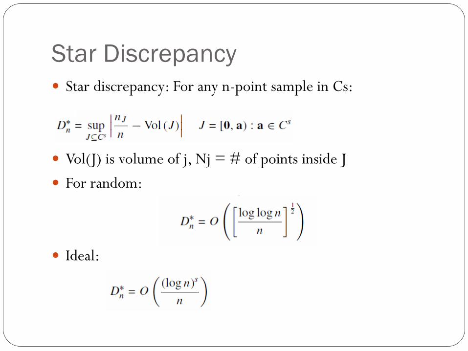
Star Discrepancy

Star discrepancy: For any n-point sample in Cs:

Vol(J) is volume of j, Nj = # of points inside J

For random:

Ideal:

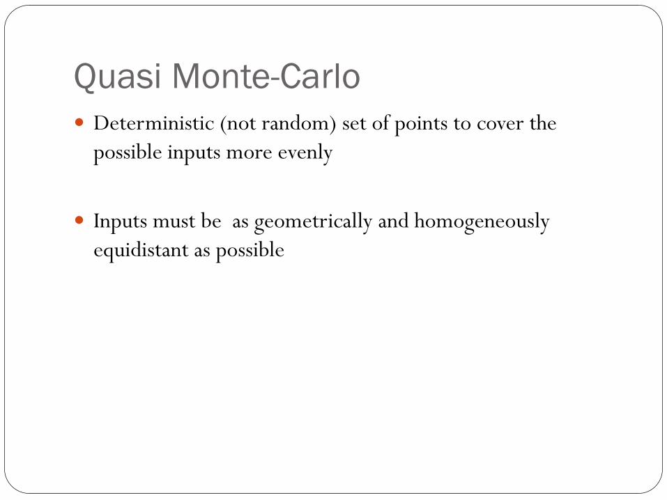
Quasi Monte-Carlo

Deterministic (not random) set of points to cover the

possible inputs more evenly

Inputs must be as geometrically and homogeneously

equidistant as possible

Sobol Point

Way of generating more uniform inputs:

Polynomial satisfies two properties w.r.t binary arithmetic

Irreducible (cannot be factored)

Smallest power P for which polynomial divides:

Sobol Continued

Direction numbers:

Subsequent direction numbers:

Compute nth sobol value

To compute nth sobol value, use this equation:

Sobol Problems Requires larger # of samples for higher dimensions for

uniformity

Despite this distribution, Quasi

Quasi-Monte-Carlo still outperforms Monte-Carlo

Latin Hypercube Sampling Variance reduction technique that reduces numerator of:

Generate N-point LHS sample over Cs:

Where are s independent and random permutations of {1,…,n}

S independent and random permutations of {1,…,n}

uij = {I = 1…n; j = 1…s} n*s random variables distributed uniformly

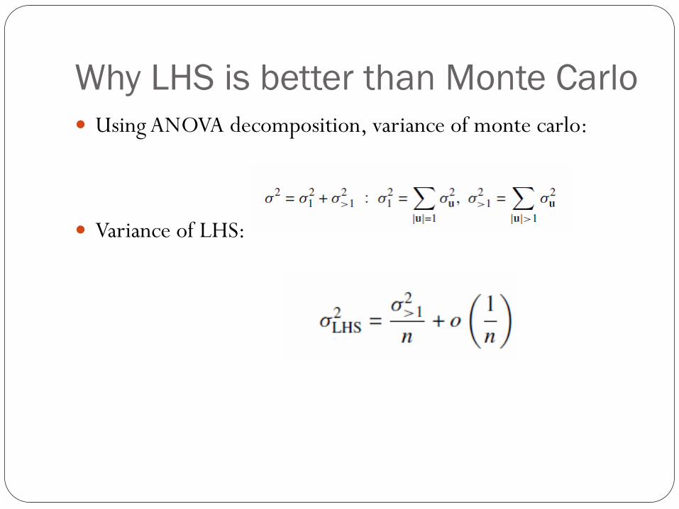
Why LHS is better than Monte Carlo

Using ANOVA decomposition, variance of monte carlo:

Variance of LHS:

Why QMC is better than LHS

Advantage of Sobol points:

Most variance contributed by 1-D ANOVA components

Significant contribution from Higher-Dimensional ANOVA

components

QMC reduces variance from 1st dimension and subsequent

dimensions

LHS reduces variance only from 1st dimension

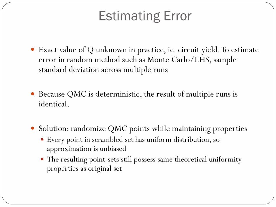
Estimating Error

Exact value of Q unknown in practice, ie. circuit yield. To estimate

error in random method such as Monte Carlo/LHS, sample standard deviation across multiple runs

Because QMC is deterministic, the result of multiple runs is identical.

Solution: randomize QMC points while maintaining properties

Every point in scrambled set has uniform distribution, so approximation is unbiased

The resulting point-sets still possess same theoretical uniformity properties as original set

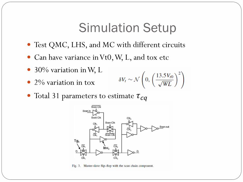
Simulation Setup

Test QMC, LHS, and MC with different circuits

Can have variance in Vt0, W, L, and tox etc

30% variation in W, L

2% variation in tox

Total 31 parameters to estimate 𝜏𝑐𝑞

64 bit SRAM

Total 403 variables

Measure write time: 𝜏𝑤

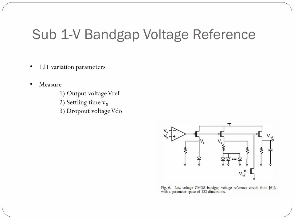
Sub 1-V Bandgap Voltage Reference

• 121 variation parameters

• Measure

1) Output voltage Vref

2) Settling time 𝜏𝑠

3) Dropout voltage Vdo

Simulation Results

Analysis of Results

QMC converges faster than Monte Carlo

LHS convergence lines are in between QMC and Monte

Carlo

A hybrid sequence sampling technique and its

application to multi-objective optimization of

blending process

Wang Shubo; Wang Yalin; Liu Bin; Gui Weihua; , "A hybrid sequence

sampling technique and its application to multi-objective optimization of

blending process," Control Conference (CCC), 2011 30th Chinese , vol., no.,

pp.2135-2140, 22-24 July 2011

URL:

http://ieeexplore.ieee.org/stamp/stamp.jsp?tp=&arnumber=6001111

&isnumber=6000362

Overview: Generating Hammersley

Sequence

2D example: Take all numbers from 0 to 2m -1 and interpret

as binary fractions. Ie. 0.00, 0.01, 0.10, 0.11.

This gives (0, ½, ¼, ¾)

Reverse bits to get second component:

(0,0), (1/2, ¼), (1/4, ½), (3/4 , ¾)

1-Dimensional Uniformity

1-Dimensional Uniformity: LHS is superior

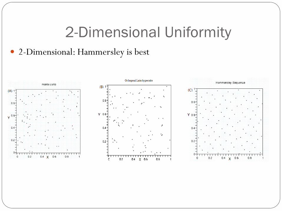
2-Dimensional Uniformity

2-Dimensional: Hammersley is best

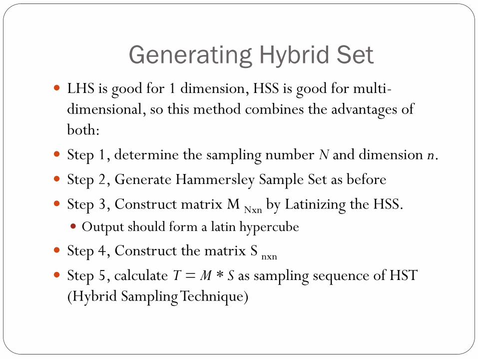
Generating Hybrid Set

LHS is good for 1 dimension, HSS is good for multi-

dimensional, so this method combines the advantages of

both:

Step 1, determine the sampling number N and dimension n.

Step 2, Generate Hammersley Sample Set as before

Step 3, Construct matrix M Nxn by Latinizing the HSS.

Output should form a latin hypercube

Step 4, Construct the matrix S nxn

Step 5, calculate T = M * S as sampling sequence of HST

(Hybrid Sampling Technique)

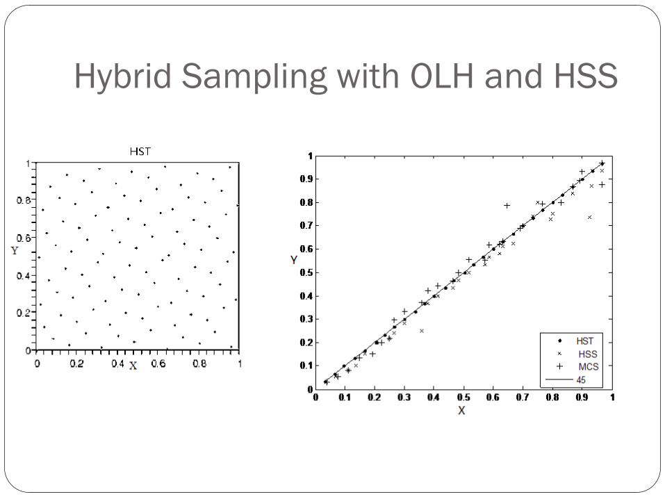
Hybrid Sampling with OLH and HSS