Monotony of Surprise and Large-Scale Quest for …stelo/papers/reco02j.pdf · Monotony of Surprise and Large-Scale Quest for Unusual Words ... user and might suggest approaches that

JOURNAL OF COMPUTATIONAL BIOLOGYVolume 10 Numbers 3ndash4 2003copy Mary Ann Liebert IncPp 283ndash311

Monotony of Surprise and Large-ScaleQuest for Unusual Words

ALBERTO APOSTOLICO1 MARY ELLEN BOCK2 and STEFANO LONARDI3

ABSTRACT

The problem of characterizing and detecting recurrent sequence patterns such as substringsor motifs and related associations or rules is variously pursued in order to compress dataunveil structure infer succinct descriptions extract and classify features etc In molecu-lar biology exceptionally frequent or rare words in bio-sequences have been implicated invarious facets of biological function and structure The discovery particularly on a mas-sive scale of such patterns poses interesting methodological and algorithmic problems andoften exposes scenarios in which tables and synopses grow faster and bigger than the rawsequences they are meant to encapsulate In previous study the ability to succinctly com-pute store and display unusual substrings has been linked to a subtle interplay betweenthe combinatorics of the subword of a word and local monotonicities of some scores used tomeasure the departure from expectation In this paper we carry out an extensive analysis ofsuch monotonicities for a broader variety of scores This supports the construction of datastructures and algorithms capable of performing global detection of unusual substrings intime and space linear in the subject sequences under various probabilistic models

Key words design and analysis of algorithms combinatoric on words statistical analysis ofsequences annotated suf x trees over- and under-represented words pattern discovery

1 INTRODUCTION AND SUMMARY

Words that occur unexpectedly often or rarely in genetic sequences have been variously linkedto biological meanings and functions The underlying probabilistic and statistical models have been

studied extensively and led to the production of a rich mass of results (see eg Reinert et al [2000]Waterman [1995]) With increasing availability of whole genomes exhaustive statistical tables and globaldetectors of unusual words on a scale of millions even billions of bases become conceivable It is naturalto ask how large such tables may grow with increasing length of the input sequence and how fast they canbe computed These problems need to be regarded not only from the conventional perspective of asymptoticspace and time complexities but also in terms of the volumes of data produced and ultimately of practicalaccessibility and usefulness Tables that are too large at the outset saturate the perceptual bandwidth of the

1Department of Computer Sciences Purdue University West Lafayette IN 47907 and Dipartimento di IngegneriadellrsquoInformazione Universitagrave di Padova Padova Italy

2Department of Statistics Purdue University West Lafayette IN 479073Department of Computer Science and Engineering University of California Riverside CA 92521

283

284 APOSTOLICO ET AL

user and might suggest approaches that sacri ce some modeling accuracy in exchange for an increasedthroughput The focus of the present paper is thus on the combinatorial structure of such tables and on thealgorithmic aspects of their implementation To make our point more clear we discuss here the problemof building exhaustive statistical tables for all subwords of very long sequences But it should becomeapparent that re ections of our arguments are met just as well in most practical cases

The number of distinct substrings in a string is at worst quadratic in the length of that string Thusthe statistical table of all words for a sequence of a modest 1000 bases may reach in principle into thehundreds of thousands of entries Such a synopsis would be asymptotically bigger than the phenomenon ittries to encapsulate or describe This is even worse than what the (now extinct) cartographers did in the oldempire narrated by Borgesrsquo ctitious JA Suagraverez Miranda (Apostolico 2001 Borges 1975) ldquoCartographyattained such perfection that the College of Cartographers evolved a Map of the Empire that was ofthe same scale as the Empire and that coincided with it point for pointrdquo1

The situation does not improve if we restrict ourselves to computing and displaying the most unusualwords in a given sequence This presupposes that we compare the frequency of occurrence of every wordin that sequence with its expectation a word that departs from expectation beyond some preset thresholdwill be labeled as unusual or surprising Departure from expectation is assessed by a distance measureoften called a score function The typical format for a z-score is that of a difference between observedand expected counts usually normalized to some suitable moment For most a priori models of a sourceit is not dif cult to come up with extremal examples of observed sequences in which the number of sayoverrepresented substrings grows itself with the square of the sequence length in such an empire a mappinpointing salient points of interest would be bigger than the empire itself Extreme as these examplesmight be they do suggest that large statistical tables may not only be computationally imposing but alsoimpractical to visualize and use thereby defying the very purpose of their construction

In this paper we study probabilistic models and scores for which the population of potentially unusualwords in a sequence can be described by tables of size at worst linear in the length of that sequence Thisnot only leads to more palatable representations for those tables but also supports (nontrivial) linear timeand space algorithms for their constructions Note that these results do not mean that now the number ofunusual words must be linear in the input but just that their representation and detection can be madesuch The ability to succinctly compute store and display our tables rests on a subtle interplay betweenthe combinatorics of the subwords of a sequence and the monotonicity of some popular scores withinsmall easily describable classes of related words Speci cally it is seen that it suf ces to consider ascandidate surprising words only the members of an a priori well identi ed set of ldquorepresentativerdquo wordswhere the cardinality of that set is linear in the text length By the representatives being identi able apriori we mean that they can be known before any score is computed By neglecting the words otherthan the representatives we are not ruling out that those words might be surprising Rather we maintainthat any such word (i) is embedded in one of the representatives and (ii) does not have a bigger scoreor degree of surprise than its representative (hence it would add no information to compute and give itsscore explicitly)

As mentioned a crucial ingredient for our construction is that the score be monotonic in each classIn this paper we perform an extensive analysis of models and scores that ful ll such a monotonicityrequirement and are thus susceptible to this treatment The main results come in the form of a series ofconditions and properties which we describe here within a framework aimed at clarifying their signi canceand scope

The paper is organized as follows Section 2 describes some preliminary notation and properties Themonotonicity results are presented in Section 3 Finally we brie y discuss the algorithmic implicationsand constructs in Section 4 We also highlight future work and extend succinct descriptors of the kindconsidered here to more general models and areas outside of the monotonicity realm These results are

1Attributed to ldquoViajes de Varones Prudentes (Libro Cuarto Cap XLV Lerida 1658)rdquo the piece ldquoOn the Exactitudeof Sciencerdquo was written in actuality by Jorge Luis Borges and Adolfo Bioy Casares English translation quoted fromBorges (1975) ldquo succeeding generations came to judge a map of such magnitude cumbersome and not withoutirreverence they abandoned it to the rigours of Sun and Rain in the whole Nation no other relic is left of theDiscipline of Geographyrdquo

MONOTONY OF SURPRISE 285

FIG 1 Overrepresented words in a set of coregulated genes A wordrsquos increasing departure from its expectedfrequency is rendered by proportionally increased font size Superposition of the words circled by hand yields thepreviously known motifs TCACGTG and AAAACTGTGG in the MET family of 11 sequences and TCCGCGGA in thePDR family of 7

being incorporated into an existing suite of programs (Lonardi 2001 Apostolico and Lonardi 2001) Asan example demonstration Fig 1 shows application of the tool to the identi cation of the core moduleswithin the regulatory regions of the yeast Finding such modules is the rst step towards a full- edgedpromoter analytic system which would help biologists to understand and investigate gene expression inrelation to development tissue speci city andor environment Each one of the two families contains aset of coregulated genes that is genes that have similar expression under the same external conditionsThe hypothesis is that in each family the upstream region will contain some common motifs and alsothat such signals might be overrepresented across the family In this like in countless other applicationsof probabilistic and statistical sequence analysis access to the widest repertoire of models and scores isthe crucial asset in the formulation testing and ne tuning of hypotheses

2 PRELIMINARIES

We use standard concepts and notation about strings for which we refer to (Apostolico et al 19982000 Apostolico and Galil 1997) For a substring y of a text x we denote by f y the number ofoccurrences of y in x We have f y D jposxyj D jendposxyj where posxy is the start-set ofstarting positions of y in x and endposxy is the similarly de ned end-set Clearly for any extensionuyv of y f uyv middot f y For a set of strings or multisequence fx1 x2 xkg the colors of y arethe members of the subset of the multisequence such that each contains at least one occurrence of y Thenumber of colors of y is denoted by cy We also have cuyv middot cy

Suppose now that string x D x[1]x[2] x[n] is a realization of a stationary ergodic random processand y[1]y[2] y[m] D y is an arbitrary but xed pattern over 6 with m lt n We de ne Zi for alli 2 [1 n iexcl m C 1] to be 1 if y occurs in x starting at position i 0 otherwise so that

Zy DniexclmC1X

iD1

Zi

is the random variable for f yExpressions for the expectation and variance for the number of occurrences in the Bernoulli model2

have been given by several authors (see eg Pevzner et al [1989] Stuumlckle et al [1990] Kleffe and

2Although ldquomultinomialrdquo would be the appropriate term for larger than binary alphabets we conform here to thecurrent usage and adopt the word ldquoBernoullirdquo throughout


Borodovsky [1992] Gentleman [1994] Reacutegnier and Szpankowski [1998]) Here we adopt derivations inApostolico et al (1998 2000) With pa the probability of symbol a 2 6 and Op D

QmiD1 py[i] we have

EZy D n iexcl m C 1 Op

VarZy Draquo

1 iexcl OpEZy iexcl Op22n iexcl 3m C 2m iexcl 1 C 2 OpBy if m middot n C 1=2

1 iexcl OpEZy iexcl Op2n iexcl m C 1n iexcl m C 2 OpBy otherwise

where

By DX

d2Py

n iexcl m C 1 iexcl d

mY

jDmiexcldC1

py[j ] (1)

is the auto-correlation factor of y that depends on the set Py of the lengths of the periods3 of y Incases of practical interest we expect m middot n C 1=2 so that we make this assumption from now on

In the case of Markov chains it is more convenient to evaluate the estimator of the expectation insteadof the true expectation to avoid computing large transition matrices In fact we can estimate the expectednumber of occurrences in the M-order Markov model with the following maximum likelihood estimator(Reinert et al 2000)

OEZy D

miexclMY

iD1

f y[iiCM]

miexclMY

iD2

f y[iiCMiexcl1]

D f y[1MC1]

miexclMY

jD2

f y[jjCM]

f y[jjCMiexcl1] (2)

The expression for the variance VarZy for Markov chains is very involved Complete derivations havebeen given by Lundstrom (1990) Kleffe and Borodovsky (1992) and Reacutegnier and Szpankowski (1998)However as soon as the true model is unknown and the transition probabilities have to be estimated fromthe observed sequence x the results for the exact distribution are no longer useful (see eg Reinert et al[2000]) In fact once we replace the expectation with an estimator of the expected count the variance ofthe difference between observed count and the estimator does not correspond anymore to the variance ofthe random variable describing the count

The asymptotic variance of EZy iexcl OEZy has been given rst by Lundstrom (1990) and is clearlydifferent from the asymptotic variance of EZy (see Waterman [1995] for a detailed exposition) Easierways to compute the asymptotic variance were also found subsequently

For a nite family fx 1 x2 xkg of realizations of our process and a pattern y we analogouslyde ne Wj for all j 2 [1 k] to be 1 if y occurs at least once in xj 0 otherwise Let

Wy DkX

jD1

Wj

so that Wy is a random variable for the total number cy of sequences which contain at least one occurrenceof y

In the case of a multisequence we can assume in actuality either a single model for the entire family ora distinct model for each sequence In any case the expectation of the random variable Wy for the numberof colors can be computed by

EWy D k iexclkX

jD1

P[Zjy D 0] (3)

because EWj D P[Zjy 6D 0]

3String z has a period w if z is a nonempty pre x of wk for some integer k cedil 1


Ideally a score function should be independent of the structure and size of the word That would allowone to make meaningful comparisons among substrings of various compositions and lengths based on thevalue of the score

There is some general consensus that z-scores may be preferred over the others (Leung et al 1996)For any word w a standardized frequency called the z-score can be de ned by

zy Df y iexcl EZy

pVarZy

If EZy and VarZy are known then under rather general conditions the statistics zy is asymptoticallynormally distributed with zero mean and unit variance as n tends to in nity In practice EZy and VarZy

are seldom known but are estimated from the sequence under studyFor a given type of count and model we consider now the problem of computing exhaustive tables

reporting scores for all substrings of a sequence or perhaps at least for the most surprising among themThe problem comes in different avors based on the probabilistic model However a table for all wordsof any size would require quadratic space in the size of the input not to mention that such a table wouldtake at least quadratic time to be lled

As seen towards the end of the paper such a limitation can be overcome by partitioning the set of allwords into equivalence classes with the property that it suf ces to account for only one or two candidatesurprising words in each class while the number of classes is linear in the textstring size More formallygiven a score function z a set of words C and a real positive threshold T we say that a word w 2 C

is T-overrepresented in C (resp T-underrepresented) if zw gt T (resp zw lt iexclT ) and for all wordsy 2 C we have zw cedil zy (resp zw middot zy) We say that a word w is T-surprising if zw gt T orzw lt iexclT We also call maxC and minC respectively the longest and the shortest word in C whenmaxC and minC are unique

Now let x be a textstring and fC1 C2 Clg a partition of all its substrings where maxCi andminCi are uniquely determined for all 1 middot i middot l For a given score z and a real positive constant T wecall O T

z the set of T -overrepresented words of Ci 1 middot i middot l with respect to that score function Similarlywe call U T

z the set of T -underrepresented words of Ci and S Tz the set of all T -surprising words 1 middot i middot l

For two strings u and v D suz a u v-path is a sequence of words fw0 D u w1 w2 wj D vgl cedil 0 such that wi is a unit-symbol extension of wiiexcl1 1 middot i middot j In general a u v-path is not uniqueIf all w 2 C belong to some minCi maxCi-path we say that class C is closed

A score function z is u v-increasing (resp nondecreasing) if given any two words w1 w2 belongingto a u v-path the condition jw1j lt jw2j implies zw1 lt zw2 (resp zw1 middot zw2) The de nitionsof a u v-decreasing and u v-nonincreasing z-scores are symmetric We also say that a score z isu v-monotonic when speci cs are unneeded or understood The following fact and its symmetric areimmediate

Fact 21 If the z-score under the chosen model is minCi maxCi-increasing and Ci is closed1 middot i middot l then

O Tz micro

l[

iD1

fmaxCig and U Tz micro

l[

iD1

fminCig

Some scores are de ned in terms of the absolute value (or any even power) of a function of expectationand count In those cases we cannot distinguish anymore overrepresented from underrepresented wordsThis restriction is compensated by the fact that we can now relax the property asked of the score functionas will be explained next

We recall that a real-valued function F is concave in a set S of real numbers if for all x1 x2 2 S andall cedil 2 0 1 we have F 1 iexcl cedilx1 C cedilx2 cedil 1 iexcl cedilF x1 C cedilF x2 If F is concave then the set ofpoints below its graph is a convex set Also given two functions F and G such that F is concave and G

is concave and monotonically decreasing we have that GF x is concaveSimilarly a function F is convex in a set S if for all x1 x2 2 S and all cedil 2 0 1 we have F 1iexclcedilx1 C

cedilx2 middot 1 iexcl cedilF x1 C cedilF x2 If F is convex then the set of points above its graph is a concave set


Also given two functions F and G such that F is convex and G is convex and monotonically increasingwe have that GF x is convex

Fact 22 If the z-score under the chosen model is a convex function of a minCi maxCi-monotonic score z0 that is

z1 iexcl cedilz0u C cedilz0v middot 1 iexcl cedilzz0u C cedilzz0v

for all u v 2 Ci and Ci is closed 1 middot i middot l then

S Tz micro

l[

iD1

fmaxCi [ minCig

This fact has two useful corollaries

Corollary 21 If the z-score under the chosen model is the absolute value of a score z0 which isminCi maxCi-monotonic and Ci is closed 1 middot i middot l then

S Tz micro

l[

iD1

fmaxCi [ minCig

Corollary 22 If the z-score under the chosen model is a convex and increasing function of a scorez0 which is in turn a convex function of a score z00 which is minCi maxCi-monotonic and Ci isclosed 1 middot i middot l then

S Tz micro

l[

iD1

fmaxCi [ minCig

An example to which the latter corollary could be applied is the choice z D z02 and z0 Dshyshyz00shyshy

Sometimes we are interested in nding words which minimize the value of a positive score instead ofmaximizing it A fact symmetric to Fact 22 also holds

Fact 23 If the z-score under the chosen model is a concave function of a minCi maxCi-monotonic score z0 that is

z1 iexcl cedilz0u C cedilz0v cedil 1 iexcl cedilzz0u C cedilzz0v

for all u v 2 Ci and Ci is closed 1 middot i middot l then the set of words for which the z-score is minimized iscontained in

l[

iD1

fmaxCi [ minCig

In the next section we present monotonicities established for a number of scores for words w and wv

that obey a condition of the form f w D f wv ie have the same set of occurrences In Section 4we discuss in more detail some of the partitions induced by such a condition with a linear number ofequivalence classes

3 MONOTONICITY RESULTS

This section displays a collection of monotonicity results established with regard to the models andz-scores considered


Recall that we consider score functions of the form

zw Df w iexcl Ew

Nw

where f w gt 0 Ew gt 0 and Nw gt 0 where Nw appears in the score as the expected value ofsome function of w

Throughout we assume w and an extension wv of w to be nonempty substrings of a text x such thatf w D f wv For convenience of notation we set frac12w acute Ew=Nw First we state a simple facton the monotonicity of Ew given the monotonicity of frac12w and Nw

Fact 31 If frac12w cedil frac12wv and if Nw gt Nwv then Ew gt Ewv

Proof From frac12w cedil frac12wv we get that Ew=Ewv cedil Nw=Nwv By hypothesis Nw=

Nwv gt 1 whence the claim

Under some general conditions on Nw and frac12w we can prove the monotonicityof any score functionsof the form described above

Theorem 31 If f w D f wv Nwv lt Nw and frac12wv middot frac12w then

f wv iexcl Ewv

Nwvgt

f w iexcl Ew

Nw

Proof By construction of the equivalence classes we have f wv D f w cedil 0 We can rewrite theinequality of the theorem as

f w

Ewv

sup31 iexcl

Nwv

Nw

acutegt 1 iexcl

frac12w

frac12wv

The left hand side is always positive because 0 lt Nwv=Nw lt 1 and the right hand size is alwaysnegative (or zero if frac12w D frac12wv)

The statement of Theorem 31 also holds by exchanging the condition frac12wv middot frac12w with f w gt

Ew gt Ewv Let us now apply the theorem to some common choices for Nw

Fact 32 If f w D f wv and Ewv lt Ew then

1 f wv iexcl Ewv gt f w iexcl Ew

2f wv

Ewvgt

f w

Ew

3f wv iexcl Ewv

Ewvgt

f w iexcl Ew

Ew

4f wv iexcl Ewv

pEwv

gtf w iexcl Ew

pEw

Proof

1 The choice Nw D 1 frac12w D Ew satis es the conditions of Theorem 31 because Ewv lt Ew2 by hypothesis 0 lt 1=Ew lt 1=Ewv and we have that f w D f wv3 the choice Nw D Ew frac12w D 1 satis es the conditions of Theorem 31 because Ewv lt Ew4 the choice Nw D

pEw frac12w D

pEw satis es the conditions of Theorem 31 because Ewv lt

Ew


Other types of scores use absolute values or powers of the difference f iexcl E

Theorem 32 If f w D f wv acute f Nwv lt Nw and frac12wv middot frac12w then

shyshyshyshyf wv iexcl Ewv

Nwv

shyshyshyshygt

shyshyshyshyf w iexcl Ew

Nw

shyshyshyshy iff f gt Ewdeg Nw C Nwv

Nw C Nwv

where deg D Ewv=Ew

Proof Note rst that 0 lt deg lt 1 by Fact 31 and that

Ewv D Ewdeg lt Ewdeg Nw C Nwv

Nw C Nwvlt Ew

We set for convenience Ecurren D Ew deg NwCNwvNwCNwv

We rst prove that if f gt Ecurren then jzwvj gt jzwj We consider two cases one of which is trivialWhen f gt Ew then both f wviexcl Ewv and f w iexcl Ew are positive and the claim follows directlyfrom Fact 32 If instead Ecurren lt f lt Ew we evaluate the difference of the scores

NwvNw jzwvj iexcl jzwj D NwvNw

sup3f iexcl deg Ew

NwvC

f iexcl Ew

Nw

acute

D f iexcl deg EwNw C f iexcl EwNwv

D f Nw C Nwv iexcl Ewdeg Nw C Nwv

D Nw C Nwvf iexcl Ecurren

which is positive by hypothesisThe converse can be proved by showing that if f middot Ecurren we have jzwvj middot jzwj Again there are two

cases one of which is trivial When 0 lt f w lt Ewv both f wv iexcl Ewv and f w iexcl Ew arenegative and the claim follows directly from Fact 32 If instead Ewv lt f middot Ecurren we use the relationobtained above ie

jzwvj iexcl jzwj DNw C Nwv

NwvNwf iexcl Ecurren

to get the claim

Theorem 32 say that these scores are monotonically decreasing when f lt Ecurren and monotonicallyincreasing when f gt Ecurren We can picture the dynamics of the score as follows Initially we can assumeEcurren gt f in which case the score is decreasing As we extend the word keeping the count f constant Ecurren

decreases (recall that Ecurren is always in the interval [Ewv Ew]) At some point Ecurren D f in which casethe score stays constant By extending the word even more Ecurren becomes smaller than f and the scorebegins to grow

Fact 33 If f w D f wv and if Ew gt Ewv acute deg Ew then

1


pEwv

shyshyshyshygt


pEw

shyshyshyshy iff f wv gt Ewp

deg

2f wv iexcl Ewv2

Ewvgt

f w iexcl Ew2

Ewiff f wv gt Ew

pdeg

Proof Relation (1) follows directly from Theorem 32 by setting Nw Dp

Ew Relation (2) followsfrom relation (1) by squaring both sides


Certain types of scores require to be minimized rather than maximized For example the scores based onthe probability that Pf w middot T or Pf w cedil T for a given threshold T on the number of occurrences

Fact 34 Given a threshold T gt 0 on the number of occurrences then

Pf w middot T middot Pf wv middot T

Proof From f uwv middot f w we know that if f w middot T then also f wv middot T Therefore Pf w middotT middot Pf wv middot T

Let us consider the score

zP w T D minfPf w middot T Pf w gt T g

D minfPf w middot T 1 iexcl Pf w middot T g

evaluated on the strings in a class C By Fact 34 one can compute the score only for the shortest and thelongest strings in C as follows

minfPf minC middot T Pf maxC gt T g

Also note that score zP w T satis es the conditions of Fact 23 In fact z0 D Pf w middot T isminC maxC-monotonic by Fact 34 and the transformation z D minfz0 1iexclz0g is a concave functionin z0

Table 1 summarizes the collection of these properties

Table 1 General Monotonicities for Scores Associated with the Counts f underthe Hypothesis f w D f wv We Have Set frac12w acute Ew=Nw and deg acute Ewv=Ew

Property Conditions

(11)f wv iexcl Ewv

Nwvgt

f w iexcl Ew

NwNwv lt Nw frac12wv middot frac12w

(12)


Nwv

shyshyshyshygt


Nw

shyshyshyshy Nwv lt Nw frac12wv middot frac12w

and f w gt Ewdeg Nw C Nwv

Nw C Nwv

(13) f wv iexcl Ewv gt f w iexcl Ew Ewv lt Ew

(14)f wv

Ewvgt

f w

EwEwv lt Ew

(15)f wv iexcl Ewv

Ewvgt

f w iexcl Ew

EwEwv lt Ew

(16)f wv iexcl Ewvp

Ewvgt

f w iexcl EwpEw

Ewv lt Ew

(17)


pEwv

shyshyshyshygt


pEw

shyshyshyshy Ew gt Ewv f w gt Ewp

deg

(18)f wv iexcl Ewv2

Ewvgt

f w iexcl Ew2

EwEw gt Ewv f w gt Ew

pdeg


31 The expected number of occurrences under Bernoulli

Let pa be the probability of the symbol a 2 6 in the Bernoulli model We de ne Op DQjwj

iD1 pw[i] and

Oq DQjvj

iD1 pv[i] Note that 0 lt pjwjmin middot Op middot p

jwjmax lt 1 where pmin D mina26 pa and pmax D maxa26 pa

We also observe that pmax cedil 1= j6j and therefore upper bounds on pmax could turn out to be unsatis ablefor small alphabets

Fact 35 Let x be a text generated by a Bernoulli process Then EZwv lt EZw

Proof We have

EZwv

EZwD

n iexcl jwj iexcl jvj C 1 Op Oqn iexcl jwj C 1 Op

Dsup3

1 iexcljvj

n iexcl jwj C 1

acuteOq lt Oq lt 1

because jvjniexcljwjC1 gt 0

Fact 36 Let x be a text generated by a Bernoulli process If f w D f wv then

1 f wv iexcl EZwv gt f w iexcl EZw

2f wv

EZwvgt

f w

EZw

3f wv iexcl EZwv

EZwvgt

f w iexcl EZw

EZw

4f wv iexcl EZwv

pEZwv

gtf w iexcl EZw

pEZw

Proof Directly from Theorem 31 and Fact 35

Fact 37 Let x be a text generated by a Bernoulli process If f w D f wv acute f then

1

shyshyshyshyf wv iexcl EZwv

pEZwv

shyshyshyshygt

shyshyshyshyf w iexcl EZw

pEZw

shyshyshyshy iff f gt EZwp

deg

2f wv iexcl EZwv2

EZwvgt

f w iexcl EZw2

EZwiff f gt EZw

pdeg

where deg D EZwv=EZw

Proof Directly from Fact 33 and Fact 35

A score that is not captured in Fact 32 uses the square root of the rst order approximation of thevariance as the normalizing factor

Fact 38 Let x be a text generated by a Bernoulli process If f w D f wv and Op lt 1=2 then

f wv iexcl EZwvpEZwv1 iexcl Op Oq

gtf w iexcl EZwp

EZw1 iexcl Op

Proof To have monotonicity the functions Nw Dp

EZw1 iexcl Op and frac12w D EZw=Nw

should satisfy the conditions of Theorem 31 First we study the ratio

sup3Nwv

Nw

acute2

Dsup3

1 iexcljvj

n iexcl jwj C 1

acuteOp Oq1 iexcl Op Oq

Op1 iexcl Oplt

Op Oq1 iexcl Op Oq

Op1 iexcl Op


The concave product Op1iexcl Op reaches its maximum for Op D 1=2 Since we assume Op lt 1=2 the rightmostterm is smaller than one The monotonicity of Nw is satis ed

Then we need to prove that frac12w also is monotonic ie frac12wv middot frac12w which is equivalent to

EZwv

EZw

1 iexcl Op1 iexcl Op Oq

middot 1

but EZwv=EZw lt 1 by hypothesis and 1 iexcl Op=1 iexcl Op Oq lt 1 for any choice of Op Oq 2 [0 1]

To study the monotonicity of the score with the complete variance we rst must prove some facts aboutthe auto-correlation function

Bw DX

d2Pw

n iexcl jwj C 1 iexcl d

jwjY

jDjwjiexcldC1

pw[j ]

where Pw is the set of the period lengths of w Throughout this section unless otherwise noted a isany of the symbols in 6 such that pa D pmax

Fact 39 Let n be the size of a text generated by a Bernoulli process and 2 middot m middot n C 1=2 Ifpa lt

p5 iexcl 1=2 then pm

a Bam is monotonically decreasing with m

Proof Words am have period set f1 2 m iexcl 1g and therefore

Bam Dmiexcl1X

lD1

n iexcl m C 1 iexcl lpla D

miexcl2X

kD0

n iexcl m iexcl kpkC1a

D n iexcl mpa

miexcl2X

kD0

pka iexcl pa

miexcl2X

kD0

kpka

D pa

sup3n iexcl m

1 iexcl pmiexcl1a

1 iexcl paiexcl

m iexcl 2pma iexcl m iexcl 1pmiexcl1

a C pa

1 iexcl pa2

acute

Dpa

1 iexcl pa2

plusmnn iexcl m1 iexcl pa1 iexcl pmiexcl1

a iexcl m iexcl 2pma C m iexcl 1pmiexcl1

a iexcl pa

sup2

Dpa

1 iexcl pa2

plusmnn iexcl m1 iexcl pa iexcl pmiexcl1

a C pma iexcl m iexcl 2pm

a C m iexcl 1pmiexcl1a iexcl pa

sup2

Dpa

1 iexcl pa2

plusmnn iexcl m iexcl n iexcl m C 1pa iexcl n iexcl 2m C 1pmiexcl1

a C n iexcl 2m C 2pma

sup2

We now consider the function bm D pma Bam in the interval n gt 0 m 2 [2 n C 1=2] pa 2 0 1

Since function bm is de ned for integer values of m we study the differences between consecutive valuesof m We de ne the function

1m acutebm iexcl 1 iexcl bm

pma

and after some algebraic manipulations we get

1m DBregmiexcl1

paiexcl Bam D iexclpm

a n iexcl 2m iexcl pmiexcl1a n iexcl 2m C 1 C n iexcl m


We rst aim our efforts towards small values of m Speci cally we look for values of pa and n suchthat b2 iexcl b3 gt 0 We have

12 Db2 iexcl b3

p3a

D iexclp2an iexcl 4 iexcl pan iexcl 3 C n iexcl 2

The solution of the inequality b2 iexcl b3 gt 0 is 0 lt pa lt 3 iexcl n Cp

5n2 iexcl 30n C 41=2n iexcl 8 Thisinterval shrinks as n grows Taking the limit n 1 we get 0 lt pa lt

p5 iexcl 1=2 frac14 0618

Repeating the analysis on b3 iexcl b4 we get

13 Db3 iexcl b4

p4a

D iexclp3an iexcl 6 iexcl p2

an iexcl 5 C n iexcl 3

which has two imaginary roots and one positive real root The function is positive in the interval 0 C2 iexcl2C C 4=6C where C D 100C 12

p69 The upper extreme of the interval is about 07548784213 which

is bigger than p

5 iexcl 1=2As we increase m the difference bmiexclbmC1 remains positive for larger and larger intervals Finally

when m D n iexcl 1=2 we get

1

sup3n iexcl 1

2

acuteD

bn iexcl 1=2 iexcl bn C 1=2

pnC1=2a

Dn C 1

2iexcl p

niexcl3=2a 2 C pa

The latter function is always positive for any choice of pa and n gt 5 In fact if n gt 5

1

sup3n iexcl 1

2

acuteD

n C 1

2iexcl p

niexcl3=2a 2 C pa cedil

n C 1

2iexcl 3 gt 0

We can conclude that the most restrictive case is m D 2 If we choose pa lt p

5 iexcl 1=2 then bm ismonotonically decreasing when 2 middot m middot n C 1=2 for any choice of n gt 0

Fact 310 Let n be the size of a text generated by a Bernoulli process and 2 middot m middot n C 1=2 Forall words w 2 6m we have

0 middot Bw middot Bam middotpa

1 iexcl pan iexcl m iexcl

p2a1 iexcl pmiexcl1

a

1 iexcl pa2

Proof We have

Bw DX

d2Pw


mY

jDmiexcldC1

pw[j ]

middotX

d2Pw

n iexcl m C 1 iexcl dpda

middotX

d2Pam


Dmiexcl1X

dD1


D Bam

since (1) all terms in the sum are positive (1 middot d middot m iexcl 1 and m middot n C 1=2) (2) am has at least all theperiods of w (ie Pw micro Pam D f1 2 m iexcl 1g) and (3)

QmjDmiexcldC1 pw[j ] middot pd

a D pdmax


From the derivation of Bam in Fact 39 we have

Bam Dpa

1 iexcl pa2



sup2

Dpa

1 iexcl pa2

plusmnn iexcl m iexcl n iexcl m C 1pa C pm

a C pmiexcl1a pa iexcl 1n iexcl 2m C 1

sup2

middotpa

1 iexcl pa2

iexcln iexcl m iexcl n iexcl m C 1pa C pm

a

cent

Dpa

1 iexcl pa

Aacuten iexcl m iexcl

miexcl1X

iD1

pia

Dpa


p2a1 iexcl pmiexcl1

a

1 iexcl pa2

because n iexcl 2m C 1 gt 0 and pa iexcl 1 middot 0

We can now get a simple bound on the maximum value achieved by OpBw for any word w 2 6C

Corollary 31 Let w be any substring of a text generated by a Bernoulli process m D jwj cedil 2 anda be the symbol in 6 such that pa D pmax lt

p5 iexcl 1=2 Then

0 middot OpBw middot n iexcl 2p3max

Proof We already know that Op middot pma and therefore OpBw middot pm

a Bw Fact 310 says that Bam isan upper bound for Bw for any word w of the same length and that pm

a Bam reach the maximum form D 2 Speci cally the maximum is p2

maxBreg2 D p2max n iexcl mpmax

We are now ready to study the monotonicity of the score with the ldquoexactrdquo variance We will warm upstudying the family of words am

Fact 311 Let 2 middot m middot n C 1=2 If pa middot 06 then VarZam is monotonically decreasing with m

Proof We study the function

VarZam D n iexcl m C 1pma 1 iexcl pm

a iexcl p2ma 2n iexcl 3m C 2m iexcl 1 C 2pm

a Bam

de ned on integer values of m We study the differences between consecutive values of m We de ne thefunction

1m acuteVarZam iexcl VarZamC1

pma

After some algebraic manipulations we get

1m D pmC2a 2nm C n iexcl 3m2 iexcl 2m iexcl pmC1

a 2n iexcl 4m

iexcl pma 2nm C n iexcl 3m2 C 1 C pan iexcl m C n iexcl m C 1

The function 1m has a root for pa D 1We rst focus our attention on the case m D 2 and study the condition VarZa2 iexclVarZa3 gt 0 We get

12 DVarZa2 iexcl VarZa3

p2a

D p4a5n iexcl 16 iexcl p3

a2n iexcl 8 iexcl p2a5n iexcl 11 C pan iexcl 2 C n iexcl 1

D pa iexcl 1plusmnp3

a5n iexcl 16 C p2a3n iexcl 8 iexcl pa2n C 3 iexcl n C 1

sup2


The four roots of this function have been computed with Maple two roots are negative one is pa D 1and one is positive pa D pcurren where pcurren is de ned below The closed form of pcurren is too long to be reportedhere We observe that function 12 is positive in the interval 0 pcurren which shrinks as n grows Forn 1 pcurren D 06056592526

Repeating the analysis for m D 3 we obtain


p3a


a2n iexcl 12 iexcl p3a7n iexcl 26 C n iexcl 2

D pa iexcl 1plusmn

p4a7n iexcl 33 C p3

a5n iexcl 21 iexcl p2a2n iexcl 5 iexcl pa2n iexcl 5 iexcl n C 2

sup2

It turns out that the interval for pa in which 13 gt 0 is larger than 0 pcurren In fact as m increases thedifference VarZam iexcl VarZamC1 becomes positive for larger and larger values of pa

Finally when m D n iexcl 1=2 we get

1

sup3n iexcl 1

2

acuteD

n C 32

Cpa

4

sup3p

nC12

a n C 12 iexcl 8pniexcl1

2a iexcl p

niexcl32

a 1 C 6n C n2 C 2n C 2

acute

and we can choose any pa in the interval 0 1 To summarize p lt 06 assures the monotonicity for alln and 2 middot m middot n C 1=2

Fact 312 For any word y and for any d 2 Py

mY

jDmiexcldC1

py[j ] DdY

jD1

py[j ]

Proof Let us decompose y D uvku where juj D d Then clearly y starts with uv and ends withvu which have the same product of probabilities under the Bernoulli model

The next three propositions are concerned with the monotonicity of the variance and the correspondingscores

Fact 313 Let w be a nonempty substring of a text generated by a Bernoulli process and wb a unitextension of w b 2 6 If pmax lt 1= m

p4m C 2 then VarZwb lt VarZw

Proof Let Ziw be the indicator random variable that w occurs in the text x at position i Then

Zw DniexclmC1X

iD1

Ziw Zwb DniexclmX

iD1

ZiwZiCmb

The proof is divided in two parts The rst is to show that VarZw gt VariexclPniexclm

iD1 Ziwcent

when pmax lt

1= mp

2m iexcl 1 Then we prove that VariexclPniexclm

iD1 Ziwcent

gt VarZwb when pmax lt 1= mp

4m C 2 Since1= m

p4m C 2 lt 1= m

p2m iexcl 1 the conclusion holds when pmax lt 1= m

p4m C 2

Let us start with the rst part We have

VarZw D Var

AacuteniexclmX

iD1

Ziw

C Op1 iexcl Op C 2niexclmX

iD1

Cov Ziw ZniexclmC1w

Due to the independence

niexclmX

iD1

Cov Ziw ZniexclmC1w DniexclmX

iDniexcl2mC2

Cov Ziw ZniexclmC1w

cedil iexclm iexcl 1 Op2


Then

VarZw iexcl Var

AacuteniexclmX

iD1

Ziw

cedil Op1 iexcl Op iexcl 2m iexcl 1 Op2

D Op1 iexcl 2m iexcl 1 Op

Since Op middot pmmax lt 1=2m iexcl 1 the rst part of the proof follows

Let us prove the second part We have

Var

AacuteniexclmX

iD1

Ziw

iexcl VarZwb D E

AacuteAacuteniexclmX

iD1

Ziw iexcl Op iexclniexclmX

iD1

ZiwZiCmb iexcl Oppb

centAacute

niexclmX

iD1

Ziw iexcl Op CniexclmX

iD1

ZiwZiCmb iexcl Oppb

DniexclmX

iD1

Cov Ziw1 iexcl ZiCmb Ziw1 C ZiCmb

CniexclmX

iD1

X

j 6Di

CoviexclZiw1 iexcl ZiCmbZj w1 C ZjCmb

cent

D n iexcl m Op1 iexcl pb iexcl Op21 iexcl p2b

C 2niexclmX

iD1

iCmX

jDiC1

plusmnEZiw1iexclZiCmbZj w1CZjCmbiexcl Op21iexclp2

bsup2

cedil n iexcl m Op1 iexcl pb1 iexcl Op1 C pb iexcl 2n iexcl mm Op21 iexcl p2b

D n iexcl m Op1 iexcl pb1 iexcl Op1 C pb iexcl 2m Op1 C pb

D n iexcl m Op1 iexcl pb1 iexcl 2m C 1 Op1 C pb

Since Op middot pmmax lt 1=4m C 2 the second part follows and also the conclusion

Fact 314 Let w be a nonempty substring of a text generated by a Bernoulli process and wb a rightextension of w b 2 6 If pmax lt

p2 iexcl 1 then EZwbp

VarZwblt EZwp

VarZw

Proof We de ne 1w b acute VarZwEZwb2 iexcl VarZwbEZw2 We have to prove 1w b lt 0We have

1w b

Op2 D VarZwp2bn iexcl m2 iexcl VarZwbn iexcl m C 12

D n iexcl m2p2bVarZw iexcl VarZwb iexcl 2n iexcl 2m C 1VarZwb

First we evaluate VarZw and we set N D n iexcl m for convenience

VarZw D OpiexclN C 11 iexcl Op iexcl 2m iexcl 1 OpN C 1 iexcl m=2 C 2Bw

cent

middot OpN C 1

Aacute

1 iexcl Op iexcl 2m iexcl 1 Op Cmm iexcl 1 Op

N C 1C 2

N C 1

miexcl1X

lD1

N C 1 iexcl lplb

D OpN C 1

Aacute

1 iexcl Opsup3

2m iexcl 1 Cmm iexcl 1

N C 1

acuteC 2

miexcl1X

lD1

sup31 iexcl

l

N C 1

acutepl

b


implies that

sup3N

N C 1

acute2 p2bVarZw

Oppbmiddot pbN

Aacute

1 iexcl Opsup3


N C 1

acuteC 2

miexcl1X

lD1

sup31 iexcl

l

N C 1

acutepl

b

Next we evaluate VarZwb

VarZwb

OppbD

sup3N1 iexcl Oppb iexcl 2 Oppb

sup3N iexcl

m C 12

acutem C 2Bwb

acute

cedil N

sup31 iexcl Oppb iexcl 2 Oppb

sup31 iexcl

m C 1

2N

acutem

acute

Note that since we are interested in the worst case for the difference VarZwiexclVarZwb we set Bwb D 0and Bw maximal This happens when w is a word of the form am where a is the symbol with the highestprobability pmax and c 6D a Recall that Fact 310 says that 0 middot Bw middot Bam Then

1w b

OppbN C 12 D

sup3N

N C 1

acute2

p2bVarZw iexcl VarZwb

Oppb

middot N

Aacute

pb iexcl Oppb

sup32m iexcl 1 iexcl

mm iexcl 1

N C 1

acuteC 2pb

miexcl1X

lD1

sup31 iexcl

l

N C 1

acutepl

b

iexcl 1 C Oppb C 2 Oppb

sup31 iexcl

m C 12N

acutem

acute

D N

Aacutepb iexcl 1 C Oppb

sup3mm iexcl 1

N C 1iexcl

mm C 1

NC 2

acuteC 2pb

miexcl1X

lD1

sup31 iexcl

l

N C 1

acutepl

b

D N

Aacute

pb iexcl 1 C Oppb

sup32 iexcl m

sup3m C 1

NN C 1C 2

N C 1

acuteacuteC 2pb

miexcl1X

lD1

sup31 iexcl

l

N C 1

acutepl

b

middot N

Aacute

pb iexcl 1 C 2 Oppb C 2pb

miexcl1X

lD1

plb

middot N

Aacute

pmax iexcl 1 C 2pmC1max C 2pmax

miexcl1X

lD1

plmax

D N

Aacute

pmax iexcl 1 C 2pmax

mX

lD1

plmax

D N

Aacute

iexclpmax C 1 C 2pmax

mX

lD0

plmax

D N1 C pmax

sup3iexcl1 C 2pmax

1 iexcl pmC1max

1 iexcl p2max

acute

We used the fact that pb middot pmax Op middot pmmax and that mC1

NNC1C 2

NC1 gt 0 A suf cient condition for thefunction 1w b to be negative is

21 iexcl pmC1max pmax middot 1 iexcl p2

max


Table 2 The Value of pcurren for Several Choices of m for Which Function 1w b

Is Negative in the Interval pmax 2 0 pcurren pcurren Converges top

2 iexcl 1

m pcurren m pcurren m pcurren

2 04406197005 5 04157303841 30 041421356243 04238537991 10 04142316092 50 041421356244 04179791697 20 04142135651 100 04142135624

Table 2 shows the root pcurren of 21 iexcl pmC1max pmax iexcl 1 C p2

max D 0 when pmax 2 [0 1] For large m itsuf ces to show that 2pmax middot 1 iexcl p2

max which corresponds to pmax middotp

2 iexcl 1

Theorem 33 Let x be a text generated by a Bernoulli process If f w D f wv and pmax lt

minf1= mp

4mp

2 iexcl 1g then

f wv iexcl EZwvp

VarZwvgt

f w iexcl EZwp

VarZw

Proof The choice Nw Dp

VarZw frac12w D Ew=p

VarZw satis es the conditions of Theo-rem 31 because the bound on pmax satis es the hypothesis of Facts 313 and 314

An interesting observation by Sinha and Tompa (2000) is that the score in Theorem 33 obeys thefollowing relation

zw middotf w iexcl EZwpEZw iexcl EZw2

when EZw iexcl EZw2 gt 0

since VarZw cedil EZw iexcl EZw2 (see Sinha and Tompa [2000] for details) It is therefore suf cientto know EZw to have an upper bound of the score If the bound happens to be smaller than than thethreshold then the algorithm can disregard that word avoiding the computation of the exact variance

Theorem 34 Let x be a text generated by a Bernoulli processIf f w D f wv acute f and pmax lt minf1= m

p4m

p2 iexcl 1g then


pVarZwv

shyshyshyshylt


pVarZw

shyshyshyshy iff f gt EZwdeg

pVarZw C

pVarZwv

pVarZw C

pVarZwv





Table 3 collects these properties

32 The expected number of occurrences under Markov models

Fact 315 Let w and v be two nonempty substrings of a text generated by a Markov process of orderM gt 0 Then OEZwv middot OEZw

Proof Let us rst prove the case M D 1 for simplicity Recall that an estimator of the expected countwhen M D 1 is given by

OEZw Df w[12]f w[23] f w[jwjiexcl1jwj]

f w[2]f w[3] f w[jwjiexcl1]


Table 3 Monotonicities for Scores Associated with the Number of Occurrences f under theBernoulli Model for the Random Variable Z We Set deg acute EZwv=EZw

Property Conditions

(21) EZwv lt EZw none

(22) f wv iexcl EZwv gt f w iexcl EZw f w D f wv

(23)f wv

EZwvgt

f w

EZwf w D f wv

(24)f wv iexcl EZwv

EZwvgt

f w iexcl EZw

EZwf w D f wv

(25)f wv iexcl EZwvp

EZwvgt

f w iexcl EZwpEZw

f w D f wv

(26)


pEZwv

shyshyshyshygt


pEZw

shyshyshyshy f w D f wv f w gt EZwp

deg

(27)f wv iexcl EZwv2

EZwvgt

f w iexcl EZw2

EZwf w D f wv f w gt EZw

pdeg


EZwv1 iexcl Op Oqgt

f w iexcl EZwpEZw1 iexcl Op

f w D f wv Op lt 1=2

(29) VarZwv lt VarZw pmax lt 1=mp

4m

(210)EZwvpVarZwv

ltEZwpVarZw

pmax ltp

2 iexcl 1


VarZwvgt

f w iexcl EZwpVarZw

f w D f wv pmax lt minf1=mp

4mp

2 iexcl 1g

(212)

shyshyshyshyf wv iexcl EZwvp

VarZwv

shyshyshyshygt

shyshyshyshyf w iexcl EZw p

VarZw

shyshyshyshy f w D f wv pmax lt minf1=mp

4mp

2 iexcl 1g

and f w gt EZwdeg

pVarZw C

pVarZwvp

VarZw Cp

VarZwv

Let us evaluate

OEZwv

OEZwD

f w[12]f w[23] f w[jwjiexcl1jwj]f w[jwj]v[1]f v[12] f v[jvjiexcl1jvj]

f w[2]f w[3] f w[jwjiexcl1]f w[jwj]f v[1] f v[jvjiexcl1]

f w[12]f w[23] f w[jwjiexcl1jwj]


Df w[jwj]v[1]f v[12] f v[jvjiexcl1jvj]

f w[jwj]f v[1] f v[jvjiexcl1]

Note that numerator and denominator have the same number of factors and that f w[jwj]v[1] middot f w[jwj]f v[12] middot f v[1] f v[jvjiexcl1jvj] middot f v[jvjiexcl1] Therefore

OEZwv

OEZwmiddot 1


Suppose now we have a Markov chain of order M gt 1 Using a standard procedure we can transformit into a Markov model of order one The alphabet of the latter is composed of symbols in one-to-onecorrespondence with all the possible substrings of length M iexcl 1

Since the argument above is independent from the size of the alphabet the conclusion holds for anyMarkov chain

Fact 316 Let x be text generated by a Markov process of order M gt 0 If f w D f wv then

1 f wv iexcl OEZwv cedil f w iexcl OEZw

2f wv

OEZwvcedil

f w

OEZw

3f wv iexcl OEZwv

OEZwvcedil

f w iexcl OEZw

OEZw

4f wv iexcl OEZwvq

OEZwv

cedilf w iexcl OEZwq

OEZw


Fact 317 Let x be text generated by a Markov process of order M gt 0 If f w D f wv acute f then

1

shyshyshyshyshyshyf wv iexcl OEZwvq

OEZwv

shyshyshyshyshyshycedil

shyshyshyshyshyshyf w iexcl OEZwq

OEZw

shyshyshyshyshyshyiff f gt EZw

pdeg

2f wv iexcl OEZwv2

OEZwvcedil

f w iexcl OEZw2

OEZwiff f gt EZw

pdeg



33 The expected number of colors for Bernoulli and Markov models

Fact 318 Let w and v be two nonempty substrings of a text generated by a any process ThenEWwv middot EWw

Proof Recall that

EWw D k iexclkX

jD1

P[Zjw D 0]

where Zjw represents the number of occurrences of the word w in th j -th sequence Since we have

P[Zjwv D 0] D P[Zj

w D 0] C P[Zjw 6D 0 and Zj

wv D 0]

then

EWw iexcl EWwv DkX

jD1

P[Zjw 6D 0 and Zj

wv D 0] cedil 0

and therefore the conclusion follows


The following three facts are a direct consequence of Fact 31 and Fact 318

Fact 319 Let x be a text generated by any process If cw D cwv then

1 cwv iexcl EWwv cedil cw iexcl EWw

2cwv

EWwvcedil

cw

EWw

3cwv iexcl EWwv

EWwvcedil

cw iexcl EWw

EWw

4cwv iexcl EWwv

EWwvcedil

cw iexcl EWw

EWw


Fact 320 Let x be a text generated by any process If cw D cwv acute c then

1

shyshyshyshycwv iexcl EWwv

pEWwv

shyshyshyshy

shyshyshyshycw iexcl EWw

pEWw

shyshyshyshy iff c gt EWwp

deg

2cwv iexcl EWwv2

EWwvcedil

cw iexcl EWw2

EWwiff c gt EWw

pdeg

where deg D EWwv=EWw


Tables 4 and 5 summarize the collection of these properties

4 COMPUTING EQUIVALENCE CLASSES AND SCORES

Here we pursue substring partitions fC1 C2 Clg in forms which would enable us to restrict thecomputation of the scores to a constant number of candidates in each class Ci Speci cally we requirefor all 1 middot i middot l maxCi and minCi to be unique Ci to be closed ie all w in Ci belong to someminCi maxCi-path and all w in Ci to have the same count Of course the partition of all substringsof x into singleton classes ful lls those properties In practice we want l to be as small as possible

We begin by recalling a few basic facts and constructs from eg Blumer et al (1987) The experiencedreader may skip most of this part We say that two strings y and w are left-equivalent on x if the set ofstarting positions of y in x matches the set of starting positions of w in x We denote this equivalencerelation by acutel It follows from the de nition that if y acutel w then either y is a pre x of w or viceversa Therefore each class has unique shortest and longest words Also by de nition if y acutel w thenf y D f w

For instance in the string ataatataataatataatatag the set fataa ataat ataatag is a left-equivalent class (with position set f1 6 9 14g) and so are ftaa taat taatag and faa aat aatag Wehave 39 left-equivalent classes much less than the total number of substrings which is 22 pound 23=2 D 253and than the number of distinct substrings in this case 61

We similarly say that y and w are right-equivalent on x if the set of ending positions of y in x matchesthe set of ending positions of w in x We denote this by acuter Finally the equivalence relation acutex is de nedin terms of the implication of a substring of x (Blumer et al 1987 Clift et al 1986) Given a substringw of x the implication impxw of w in x is the longest string uwv such that every occurrence of w inx is preceded by u and followed by v We write y acutex w iff impxy D impxw It is not dif cult to seethe following


Table 4 Monotonicities for Scores Associated with the Number of Occurrences f

under Markov Model for the Random Variable Z We Set deg acute EZwv=EZw

Property Conditions

(31) OEZwv middot OEZw none

(32) f wv iexcl OEZwv cedil f w iexcl OEZw f w D f wv

(33)f wv

OEZwvcedil f w

OEZwf w D f wv

(34)f wv iexcl OEZwv

OEZwvcedil f w iexcl OEZw

OEZwf w D f wv

(35)f wv iexcl OEZwvq

OEZwv


OEZw

f w D f wv

(36)


OEZwv


shyshyshyshyshyshyf w iexcl OEZw q

OEZw

shyshyshyshyshyshyf w D f wv f w gt EZw

pdeg

(37)f wv iexcl OEZwv2

OEZwvcedil f w iexcl OEZw2

OEZwf w D f wv f w gt EZw

pdeg

Table 5 Monotonicities of the Scores Associated with the Number of Colors c

under Any Model for the Random Variable W We Set deg acute EWwv=EWw

Property Conditions

(41) EWwv middot EWw none

(42) cwv iexcl EWwv cedil cw iexcl EWw cw D cwv

(43)cwv

EWwvcedil cw

EWwcw D cwv

(44)cwv iexcl EWwv

EWwvcedil cw iexcl EWw

EWwcw D cwv

(45)cwv iexcl EWwv

pEWwv

cedilcw iexcl EWw

pEWw

cw D cwv

(46)


pEWwv

shyshyshyshy


pEWw

shyshyshyshy cw D cwv cw gt EWw p

deg

(47)cwv iexcl EWwv2

EWwvcedil cw iexcl EWw2

EWwcw D cwv cw gt EWw

pdeg


Lemma 41 The equivalence relation acutex is the transitive closure of acutel [ acuter

More importantly the size l of the partition is linear in jxj D n for all three equivalence relationsconsidered In particular the smallest size is attained by acutex for which the number of equivalence classesis at most n C 1

Each one of the equivalence classes discussed can be mapped to the nodes of a corresponding automatonor word graph which becomes thereby the natural support for our statistical tables The table takes linearspace since the number of classes is linear in jxj The automata themselves are built by classical algorithmsfor which we refer to eg Apostolico et al (2000) Apostolico and Galil (1997) and Blumer et al (1987)with their quoted literature or easy adaptations thereof The graph for acutel for instance is the compactsubword tree Tx of x whereas the graph for acuter is the dawg or directed acyclic word graph Dx for xThe graph for acutex is the compact version of the the dawg

These data structures are known to commute in simple ways so that say an acutex-class can be foundon Tx as the union of some left-equivalent classes or alternatively as the union of some right-equivalentclasses Following are some highlights for the inexperienced reader Beginning with left-equivalent classesthat correspond one-to-one to the nodes of Tx we can build some right-equivalent classes as follows Weuse the elementary fact that whenever there is a branching node sup1 in Tx corresponding to w D ay a 2 6then there is also a node ordm corresponding to y and there is a special suf x link directed from ordm to sup1Such auxiliary links induce another tree on the nodes of Tx that we may call Sx It is now easy to nd aright-equivalent class with the help of suf x links For this we traverse Sx bottom-up while grouping in asingle class all strings such that their terminal nodes in Tx are roots of isomorphic subtrees of Tx Whena subtree that violates the isomorphism condition is encountered we are at the end of one class and westart with a new one

For example the three subtrees rooted at the solid nodes in Fig 2 correspond to the end-sets of ataatataata and aata which are the same namely f6 11 14 19g These three words de ne the right-equivalent class fataata taata aatag In fact this class cannot be made larger because the two

FIG 2 The tree Tx for x D ataatataataatataatatag subtrees rooted at the solid nodes are isomorphic


subtrees rooted at the end nodes of ata and tataata are not isomorphic to the substree of the classWe leave it as an exercise for the reader to nd all the right-equivalence classes on Tx It turns out thatthere are 24 such classes in this example

Subtree isomorphism is checked by a classical linear-time algorithm by Aho et al (1974) But on Tx

this is done even more quickly once the f counts are available (Apostolico and Lonardi 2002 Gus eld1997)

Lemma 42 Let T1 and T2 be two subtrees of Tx T1 and T2 are isomorphic if and only if they havethe same number of leaves and their roots are connected by a chain of suf x links

Proof If T1 and T2 are isomorphic then clearly they have same number of leaves Also if they werenot linked by a chain of suf x links strings w1 and w2 corresponding to the path-labels of the roots ofT1 and T2 could not be a suf x of one another Hence their end-sets would be different contrary to thehypothesis of the isomorphism of the subtrees T1 and T2

Let us assume wlog that there is a chain formed by l suf x links from the root of T1 to the root ofT2 l cedil 1 Let uw be the path-label for the root of T1 and w the path-label for the root of T2 whencel D juj In general we have that endposuw micro endposw Since we know that f uw D f w thenthe only possibility is that endposuw D endposw hence the subtrees are isomorphic

If during the bottom-up traversal of Sx we put in the same class strings such that their terminal arcleads to nodes with the same frequency counts f then this would identify and produce the acutex -classesie the smallest substring partition

For instance starting from the right-equivalent class C D fataata taata aatag one can aug-ment it with of all words which are left-equivalent to the elements of C The result is one acutex -classcomposed by fataa ataat ataata taa taat taata aa aat aatag Their respective pos

sets are f1 6 9 14g f1 6 9 14g f1 6 9 14g f2 7 10 15g f2 7 10 15g f2 7 10 15g f3 8 11 16gf3 8 11 16g f3 8 11 16g Their respective endpos sets are f4 9 12 17g f5 10 13 18g f6 11 14 19gf4 9 12 17g f5 10 13 18g f6 11 14 19g f4 9 12 17g f5 10 13 18g f6 11 14 19g Because ofLemma 41 given two words y and w in the class either they share the start set or they share theend set or they share the start set by transitivity with a third word in the class or they share the end set bytransitivity with a third word in the class It turns out that there are only seven acutex -classes in our example

Note that the longest string in this acutex -class is unique (ataata) and that it contains all the othersas substrings The shortest string is unique as well (aa) As said the number of occurrences for all thewords in the same class is the same (four in the example) Figure 3 illustrates the seven equivalenceclasses for our running example The words in each class have been organized in a lattice where edgescorrespond to extensions (or contractions) of a single symbol In particular horizontal edges correspondto right extensions and vertical edges to left extensions

While the longest word in an acutex -class is unique there may be in general more than one shortestword Consider for example the text x D akgk with k gt 0 (see Fig 4) Choosing k D 2 yields aclass which has three words of length two as minimal elements namely aa gg and ag (In factimpxaa D impxgg D impxag D aagg) Taking instead k D 1 all three substrings of x D ag

coalesce into a single class which has two shortest wordsWe recall that by Lemma 41 each acutex -class C can be expressed as the union of one or more left-

equivalent classes Alternatively C can be also expressed as the union of one or more right-equivalentclasses The example above shows that there are cases in which we cannot merge left- or right-equivalentclasses without violating the uniqueness of the shortest word Thus we may use the acutex -classes as the Ci rsquosin our partition only if we are interested in detecting overrepresented words If underrepresented words arealso wanted then we must represent the same acutex -class once for each distinct shortest word in it

It is not dif cult to accommodate this in our subtree merge procedure Let pu denote the parent of u

in Tx While traversing Sx bottom-up we merge two nodes u and v with the same f count if and onlyif u and v are connected by a suf x link and pu and pv are also This results in a substring partitionslightly coarser acutex which will be denoted by Qx In conclusion we can state the following fact


FIG 3 A representation of the seven acutex -classes for x D ataatataataatataatatag The words in each classcan be organized in a lattice Numbers refer to the number of occurrences

FIG 4 One acutex-class for the string x D aktk


Fact 41 Let fC1 C2 Clg be the set of equivalence classes built on the equivalence relation Qx

on the substrings of text x Then for all 1 middot i middot l

1 maxCi and minCi are unique2 all w 2 Ci are on some minCi maxCi-path3 all w 2 Ci have the same number of occurrences f w

4 all w 2 Ci have the same number of colors cw

We are now ready to address the computational complexity of our constructions In Apostolico et al(2000) linear-time algorithms are given to compute and store expected value EZ and variance VarZ

for the number of occurrences under the Bernoulli model of all pre xes of a given string The crux ofthat construction rests on deriving an expression of the variance (see Expression 1) that can be cast withinthe classical linear time computation of the ldquofailure functionrdquo or smallest periods for all pre xes of astring (see eg Aho et al [1974]) These computations are easily adapted to be carried out on the linkedstructure of graphs such as Sx or Dx thereby yielding expectation and variance values at all nodes of Tx Dx or the compact variant of the latter These constructions take time and space linear in the size of thegraphs hence linear in the length of x Combined with our monotonicity results this yields immediately

Theorem 41 Under the Bernoulli models the sets O Tz and U T

z for scores

z1w D f w iexcl EZw

z2w Df w

EZw

z3w Df w iexcl EZw

EZw

z4w Df w iexcl EZw

pEZw

z5w Df w iexcl EZwp

EZw1 iexcl Opwhen Op lt 1=2

z6w Df w iexcl EZw

pVarZw

when pmax lt minf1=mp

4mp

2 iexcl 1g

and the set S Tz for scores

z7w Dshyshyshyshyf w iexcl EZw

pEZw

shyshyshyshy

z8w Df w iexcl EZw2

EZw


pVarZw

shyshyshyshywhen pmax lt minf1=mp

4mp

2 iexcl 1g

can be computed in linear time and space

The computation of OEZy is more involved in Markov models than with Bernoulli Recall from Ex-pression 2 that the maximum likelihood estimator for the expectation is

OEZy D f y[1MC1]

miexclMY

jD2

f y[jjCM]

f y[jjCMiexcl1]


where M is the order of the Markov chain If we compute the (Markov) pre x product ppi as

ppi D

8gtgtlt

gtgt

1 if i D 0

iY

jD1

f x[jjCM]

f x[jjCMiexcl1]if 1 middot i middot n

then OEZy is rewrittten as

OEZy D f y[1MC1]ppe iexcl M

ppb

where b e gives the beginning and the ending position of any of the occurrences of y in x Hence iff y[1MC1] and the vector ppi are available we can compute OEZy in constant time

It is not dif cult to compute the auxiliary products ppi in overall linear time eg beginning at thenode of Tx which is found at the end of the path to x[1MC1] and then alternating between suf x- and directedge transitions on the tree We leave the details for an exercise When working with multisequences wehave to build a vector of pre x products for each sequence using the global statistics of occurrences ofeach word of size M and M C 1 We also build the Bernoulli pre x products to compute EZ for wordssmaller than M C2 because the estimator of OEZ cannot be used for these words The resulting algorithmis linear in the total size of the multisequence

The following theorem summarizes these results

Theorem 42 Under Markov models the sets O Tz and U T

z for scores

z11w D f w iexcl OEZw

z12w Df w

OEZw

z13w Df w iexcl OEZw

OEZw

z14w Df w iexcl OEZwq

OEZw



pEZw

shyshyshyshy

z16w Df w iexcl EZw2

EZw


We now turn to color counts in multisequences The computation of EW and VarW can be ac-complished once array fEZ

jy j 2 [1 k]g that is the expected number of occurrences of y in each

sequence is available EZjy has to be evaluated on the local model estimated only from the j -th sequence

Once all EZjy are available we can use Equation 3 to compute EWy and VarWy

Having k different sets of parameters to handle makes the usage of the pre x products slightly moreinvolved For any word y we have to estimate its expected number of occurrences in each sequence evenin sequences in which y does not appear at all Therefore we cannot compute only one pre x product foreach sequence We need to compute k vectors of pre x products for each sequence at an overall Okn

time and space complexity for the preprocessing phase where we assume n DPk

iD1

shyshyxishyshy We need an


additional vector in which we record the starting position of any of the occurrences of y in each sequenceThe resulting algorithm has overall time complexity Okn

The following theorem summarizes this discussion

Theorem 43 Under any model the sets O Tz and U T

z of a multisequence fx1 x2 xkg forscores

z17w D cw iexcl EWw

z18w Dcw

EWw

z19w Dcw iexcl EWw

EWw

z20w Dcw iexcl EWw

pEWw


z21w Dshyshyshyshycw iexcl EWw

pEWw

shyshyshyshy

z22w Dcw iexcl EWw2

EWw

can be computed in Oplusmnk

PkiD1

shyshyxishyshysup2

time and space

5 CONCLUSIONS

We have shown that under several scores and models we can bound the number of candidate over- andunderrepresented words in a sequence and carry out the related computations in correspondingly ef cienttime and space Our results require that the scores under consideration grow monotonically for words ineach class of a partition of which the index or number of classes is linear in the textstring As seen in thispaper such a condition is met by many scores The corresponding statistical tables take up the form ofsome variant of a trie structure of which the branching nodes in a number linear in the textstring lengthare all and only the sites where a score needs be computed and displayed In practice additional spacesavings could achieved by grouping in a same equivalence class consecutive branching nodes in a chainof nodes in which the scores are nondecreasing For instance this could be based on the condition that thedifference of observed and expected frequency is larger for the longer word and the normalization termis decreasing for the longer word (The case of xed frequency for both words is just a special case ofthis) Note that in such a variant of the trie the words in an equivalence class are no longer characterizedby having essentially the same list of occurrences Another way of giving the condition is to say that theratio of the frequency of the longer word to that of the shorter word should be larger than the ratio of theircorresponding expectations In this case the longer word has the bigger score Still an important questionregards more the generation of tables for general scores particularly for those that do not necessarilymeet those monotonicity conditions There are two quali cations to the problem respectively regardingspace and construction time As far as space is concerned we have seen that the crucial handle towardslinear space is represented by equivalence class partitions fC1 C2 Clg that satisfy properties such asin Fact 41 Clearly the equivalence relations acutel acuter and Qx all meet these conditions We note that aclass Ci in any of the corresponding partitions represents a maximal set of strings that occur precisely atthe same positions in x possibly up to some small uniform offset For our purposes any such class maybe fully represented by the quadruplet fmaxCi minCi i1 l1 zmax i2 l2 zming where i1 l1 zmax

and i2 l2 zmin give the positions lengths and scores of the substrings of maxCi achieving the largestand smallest score values respectively The monotonicity conditions studied in this paper automatically


assign zmax to maxCi and zmin to minCi thereby rendering redundant the position information in aquadruplet In addition when dealing with acutel (respectively acuter ) we also know that minCi is a pre x(respectively suf x) of maxCi which brings even more savings In the general case a linear number ofquadruplets such as above fully characterizes the set of unusual words This is true in particular for thepartition associated with the equivalence relation Qx which achieves the smallest number of classes underthe constrains of Fact 41 The corresponding graph may thus serve as the natural support of exhaustivestatistical tables for the most general models The computational costs involved in producing such tablesmight pose further interesting problems of algorithm design

ACKNOWLEDGMENTS

The passage by JL Borges which inspired the title of Apostolico (2001) was pointed out to the authorby Gustavo Stolovitzky We are also grateful to the referees for their helpful comments In particular wethank one of the referees for suggesting an alternative proof of Fact 313 Dan Gus eld brought to ourattention that Lemma 42 had been previously established by Gus eld (1997)

REFERENCES

Aho AV Hopcroft JE and Ullman JD 1974 The Design and Analysis of Computer Algorithms Addison-WesleyReading MA

Apostolico A 2001 Of maps bigger than the empire Keynote in Proc 8th Int Colloquium on String Processing andInformation Retrieval (Laguna de San Rafael Chile November 2001) IEEE Computer Society Press

Apostolico A Bock ME Lonardi S and Xu X 2000 Ef cient detection of unusual words J Comp Biol 7(1ndash2)71ndash94

Apostolico A Bock ME and Xu X 1998 Annotated statistical indices for sequence analysis in Carpentieri BDe Santis A Vaccaro U and Storer J eds Compression and Complexity of Sequences pp 215ndash229 IEEEComputer Society Press Positano Italy

Apostolico A and Galil Z eds 1997 Pattern Matching Algorithms Oxford University Press New YorkApostolico A and Lonardi S 2001 Verbumculus wwwcsucreduraquosteloVerbumculusApostolico A and Lonardi S 2002 A speed-up for the commute between subword trees and DAWGs Information

Processing Letters 83(3) 159ndash161Blumer A Blumer J Ehrenfeucht A Haussler D and McConnel R 1987 Complete inverted les for ef cient

text retrieval and analysis J Assoc Comput Mach 34(3) 578ndash595Borges JL 1975 A Universal History of Infamy Penguin Books LondonClift B Haussler D McConnell R Schneider TD and Stormo GD 1986 Sequences landscapes Nucl Acids

Res 14 141ndash158Gentleman J 1994 The distribution of the frequency of subsequences in alphabetic sequences as exempli ed by

deoxyribonucleic acid Appl Statist 43 404ndash414Gus eld D 1997 Algorithms on Strings Trees and Sequences Computer Science and Computational Biology

Cambridge University Press LondonKleffe J and Borodovsky M 1992 First and second moment of counts of words in random texts generated by

Markov chains Comput Appl Biosci 8 433ndash441Leung MY Marsh GM and Speed TP 1996 Over and underrepresentation of short DNA words in herpesvirus

genomes J Comp Biol 3 345ndash360Lonardi S 2001 Global Detectors of Unusual Words Design Implementation and Applications to Pattern Discovery

in Biosequences PhD Thesis Department of Computer Sciences Purdue UniversityLundstrom R 1990 Stochastic models and statistical methods for DNA sequence data PhD Thesis University of

UtahPevzner PA Borodovsky MY and Mironov AA 1989 Linguistics of nucleotides sequences I The signi cance of

deviations from mean statistical characteristics and prediction of the frequencies of occurrence of words J BiomolStruct Dyn 6 1013ndash1026

Reacutegnier M and Szpankowski W 1998 On pattern frequency occurrences in a Markovian sequence Algorithmica22 631ndash649

Reinert G Schbath S and Waterman MS 2000 Probabilistic and statistical properties of words An overviewJ Comp Biol 7 1ndash46


Sinha S and Tompa M 2000 A statistical method for nding transcription factor binding sites Proc 8th Int ConfIntelligent Systems for Molecular Biology 344ndash354

Stuumlckle E Emmrich C Grob U and Nielsen P 1990 Statistical analysis of nucleotide sequences Nucl AcidsRes 18(22) 6641ndash6647

Waterman MS 1995 Introduction to Computational Biology Chapman and Hall London

Address correspondence toAlberto Apostolico

Department of Computer SciencesPurdue University

Computer Sciences BuildingWest Lafayette IN 47907

E-mail axacspurdueedu


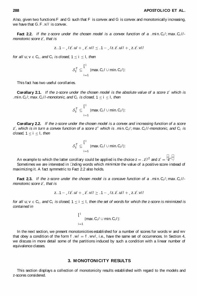
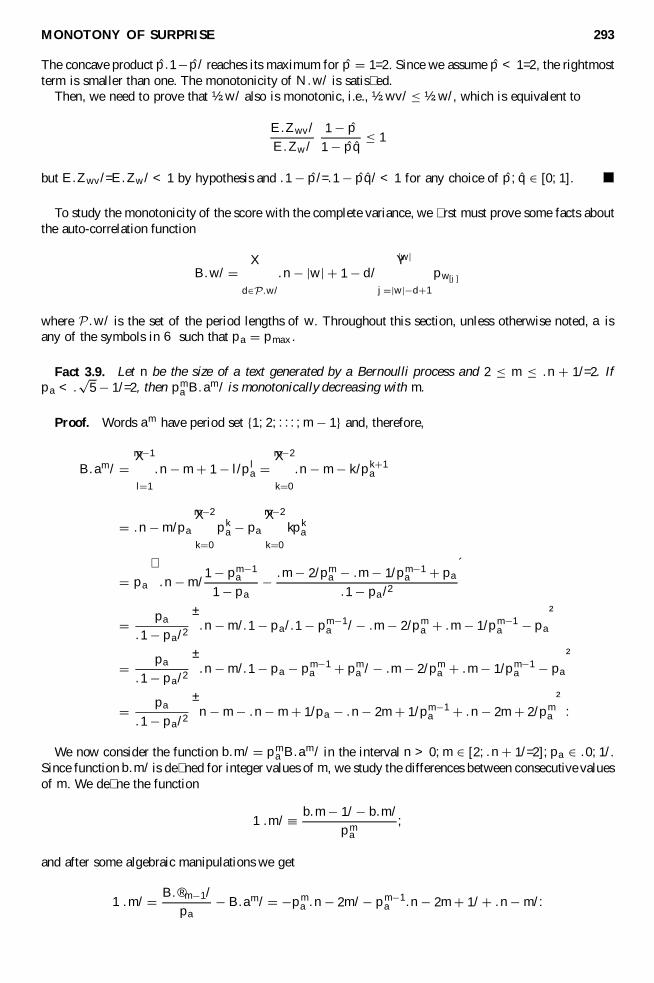
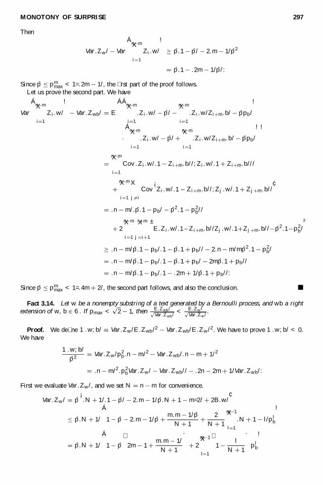
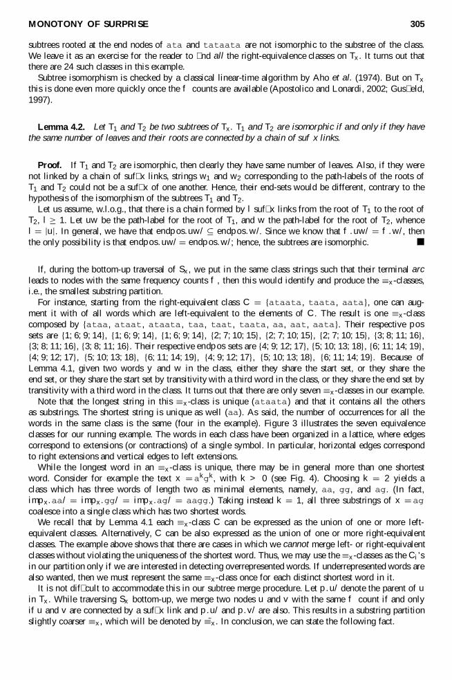user and might suggest approaches that sacri ce some modeling accuracy in exchange for an increasedthroughput The focus of the present paper is thus on the combinatorial structure of such tables and on thealgorithmic aspects of their implementation To make our point more clear we discuss here the problemof building exhaustive statistical tables for all subwords of very long sequences But it should becomeapparent that re ections of our arguments are met just as well in most practical cases

The number of distinct substrings in a string is at worst quadratic in the length of that string Thusthe statistical table of all words for a sequence of a modest 1000 bases may reach in principle into thehundreds of thousands of entries Such a synopsis would be asymptotically bigger than the phenomenon ittries to encapsulate or describe This is even worse than what the (now extinct) cartographers did in the oldempire narrated by Borgesrsquo ctitious JA Suagraverez Miranda (Apostolico 2001 Borges 1975) ldquoCartographyattained such perfection that the College of Cartographers evolved a Map of the Empire that was ofthe same scale as the Empire and that coincided with it point for pointrdquo1

The situation does not improve if we restrict ourselves to computing and displaying the most unusualwords in a given sequence This presupposes that we compare the frequency of occurrence of every wordin that sequence with its expectation a word that departs from expectation beyond some preset thresholdwill be labeled as unusual or surprising Departure from expectation is assessed by a distance measureoften called a score function The typical format for a z-score is that of a difference between observedand expected counts usually normalized to some suitable moment For most a priori models of a sourceit is not dif cult to come up with extremal examples of observed sequences in which the number of sayoverrepresented substrings grows itself with the square of the sequence length in such an empire a mappinpointing salient points of interest would be bigger than the empire itself Extreme as these examplesmight be they do suggest that large statistical tables may not only be computationally imposing but alsoimpractical to visualize and use thereby defying the very purpose of their construction

In this paper we study probabilistic models and scores for which the population of potentially unusualwords in a sequence can be described by tables of size at worst linear in the length of that sequence Thisnot only leads to more palatable representations for those tables but also supports (nontrivial) linear timeand space algorithms for their constructions Note that these results do not mean that now the number ofunusual words must be linear in the input but just that their representation and detection can be madesuch The ability to succinctly compute store and display our tables rests on a subtle interplay betweenthe combinatorics of the subwords of a sequence and the monotonicity of some popular scores withinsmall easily describable classes of related words Speci cally it is seen that it suf ces to consider ascandidate surprising words only the members of an a priori well identi ed set of ldquorepresentativerdquo wordswhere the cardinality of that set is linear in the text length By the representatives being identi able apriori we mean that they can be known before any score is computed By neglecting the words otherthan the representatives we are not ruling out that those words might be surprising Rather we maintainthat any such word (i) is embedded in one of the representatives and (ii) does not have a bigger scoreor degree of surprise than its representative (hence it would add no information to compute and give itsscore explicitly)

As mentioned a crucial ingredient for our construction is that the score be monotonic in each classIn this paper we perform an extensive analysis of models and scores that ful ll such a monotonicityrequirement and are thus susceptible to this treatment The main results come in the form of a series ofconditions and properties which we describe here within a framework aimed at clarifying their signi canceand scope

The paper is organized as follows Section 2 describes some preliminary notation and properties Themonotonicity results are presented in Section 3 Finally we brie y discuss the algorithmic implicationsand constructs in Section 4 We also highlight future work and extend succinct descriptors of the kindconsidered here to more general models and areas outside of the monotonicity realm These results are

1Attributed to ldquoViajes de Varones Prudentes (Libro Cuarto Cap XLV Lerida 1658)rdquo the piece ldquoOn the Exactitudeof Sciencerdquo was written in actuality by Jorge Luis Borges and Adolfo Bioy Casares English translation quoted fromBorges (1975) ldquo succeeding generations came to judge a map of such magnitude cumbersome and not withoutirreverence they abandoned it to the rigours of Sun and Rain in the whole Nation no other relic is left of theDiscipline of Geographyrdquo




2 PRELIMINARIES



Zy DniexclmC1X

iD1

Zi






QmiD1 py[i] we have


VarZy Draquo



where

By DX

d2Py


mY

jDmiexcldC1

py[j ] (1)



OEZy D

miexclMY

iD1

f y[iiCM]

miexclMY

iD2

f y[iiCMiexcl1]

D f y[1MC1]

miexclMY

jD2

f y[jjCM]

f y[jjCMiexcl1] (2)




Wy DkX

jD1

Wj



EWy D k iexclkX

jD1

P[Zjy D 0] (3)






zy Df y iexcl EZy

pVarZy












O Tz micro

l[

iD1


l[

iD1

fminCig










S Tz micro

l[

iD1

fmaxCi [ minCig



S Tz micro

l[

iD1

fmaxCi [ minCig


S Tz micro

l[

iD1

fmaxCi [ minCig






l[

iD1

fmaxCi [ minCig







zw Df w iexcl Ew

Nw








f wv iexcl Ewv

Nwvgt

f w iexcl Ew

Nw


f w

Ewv

sup31 iexcl

Nwv

Nw

acutegt 1 iexcl

frac12w

frac12wv






2f wv

Ewvgt

f w

Ew

3f wv iexcl Ewv

Ewvgt

f w iexcl Ew

Ew

4f wv iexcl Ewv

pEwv

gtf w iexcl Ew

pEw

Proof


pEw frac12w D


Ew





Nwv

shyshyshyshygt


Nw


Nw C Nwv

where deg D Ewv=Ew



Nw C Nwvlt Ew




sup3f iexcl deg Ew

NwvC

f iexcl Ew

Nw

acute








to get the claim




1


pEwv

shyshyshyshygt


pEw


deg

2f wv iexcl Ewv2

Ewvgt

f w iexcl Ew2

Ewiff f wv gt Ew

pdeg
















Property Conditions

(11)f wv iexcl Ewv

Nwvgt

f w iexcl Ew


(12)


Nwv

shyshyshyshygt


Nw



Nw C Nwv


(14)f wv

Ewvgt

f w

EwEwv lt Ew

(15)f wv iexcl Ewv

Ewvgt

f w iexcl Ew

EwEwv lt Ew

(16)f wv iexcl Ewvp

Ewvgt

f w iexcl EwpEw

Ewv lt Ew

(17)


pEwv

shyshyshyshygt


pEw


deg

(18)f wv iexcl Ewv2

Ewvgt

f w iexcl Ew2


pdeg




iD1 pw[i] and

Oq DQjvj





Proof We have

EZwv

EZwD


Dsup3

1 iexcljvj

n iexcl jwj C 1

acuteOq lt Oq lt 1




2f wv

EZwvgt

f w

EZw

3f wv iexcl EZwv

EZwvgt

f w iexcl EZw

EZw

4f wv iexcl EZwv

pEZwv

gtf w iexcl EZw

pEZw



1


pEZwv

shyshyshyshygt


pEZw


deg

2f wv iexcl EZwv2

EZwvgt

f w iexcl EZw2

EZwiff f gt EZw

pdeg






gtf w iexcl EZwp

EZw1 iexcl Op




sup3Nwv

Nw

acute2

Dsup3

1 iexcljvj

n iexcl jwj C 1


Op1 iexcl Oplt

Op Oq1 iexcl Op Oq

Op1 iexcl Op




EZwv

EZw


middot 1



Bw DX

d2Pw


jwjY

jDjwjiexcldC1

pw[j ]






Bam Dmiexcl1X

lD1


miexcl2X

kD0


D n iexcl mpa

miexcl2X

kD0

pka iexcl pa

miexcl2X

kD0

kpka

D pa

sup3n iexcl m

1 iexcl pmiexcl1a

1 iexcl paiexcl


a C pa

1 iexcl pa2

acute

Dpa

1 iexcl pa2



a iexcl pa

sup2

Dpa

1 iexcl pa2




sup2

Dpa

1 iexcl pa2



sup2




pma


1m DBregmiexcl1





12 Db2 iexcl b3

p3a






13 Db3 iexcl b4

p4a





is bigger than p



1

sup3n iexcl 1

2

acuteD


pnC1=2a

Dn C 1

2iexcl p

niexcl3=2a 2 C pa


1

sup3n iexcl 1

2

acuteD

n C 1

2iexcl p


n C 1

2iexcl 3 gt 0






p2a1 iexcl pmiexcl1

a

1 iexcl pa2

Proof We have

Bw DX

d2Pw


mY

jDmiexcldC1

pw[j ]

middotX

d2Pw


middotX

d2Pam


Dmiexcl1X

dD1


D Bam



a D pdmax



Bam Dpa

1 iexcl pa2



sup2

Dpa

1 iexcl pa2



sup2

middotpa

1 iexcl pa2


a

cent

Dpa

1 iexcl pa


miexcl1X

iD1

pia

Dpa


p2a1 iexcl pmiexcl1

a

1 iexcl pa2




p5 iexcl 1=2 Then











a Bam



pma



a 2n iexcl 4m




p2a





sup2





p3a



D pa iexcl 1plusmn

p4a7n iexcl 33 C p3


sup2



1

sup3n iexcl 1

2

acuteD

n C 32

Cpa

4

sup3p

nC12


2a iexcl p

niexcl32

a 1 C 6n C n2 C 2n C 2

acute



mY

jDmiexcldC1

py[j ] DdY

jD1

py[j ]






Zw DniexclmC1X

iD1

Ziw Zwb DniexclmX

iD1

ZiwZiCmb


iD1 Ziwcent

when pmax lt

1= mp


iD1 Ziwcent


4m C 2 Since1= m

p4m C 2 lt 1= m


p4m C 2


VarZw D Var

AacuteniexclmX

iD1

Ziw


iD1

Cov Ziw ZniexclmC1w


niexclmX

iD1


iDniexcl2mC2

Cov Ziw ZniexclmC1w



Then

VarZw iexcl Var

AacuteniexclmX

iD1

Ziw





Var

AacuteniexclmX

iD1

Ziw

iexcl VarZwb D E


iD1


iD1

ZiwZiCmb iexcl Oppb

centAacute

niexclmX

iD1


iD1

ZiwZiCmb iexcl Oppb

DniexclmX

iD1


CniexclmX

iD1

X

j 6Di


cent


C 2niexclmX

iD1

iCmX

jDiC1


bsup2







VarZwblt EZwp

VarZw


1w b





cent

middot OpN C 1

Aacute


N C 1C 2

N C 1

miexcl1X

lD1

N C 1 iexcl lplb

D OpN C 1

Aacute

1 iexcl Opsup3


N C 1

acuteC 2

miexcl1X

lD1

sup31 iexcl

l

N C 1

acutepl

b


implies that

sup3N

N C 1

acute2 p2bVarZw

Oppbmiddot pbN

Aacute

1 iexcl Opsup3


N C 1

acuteC 2

miexcl1X

lD1

sup31 iexcl

l

N C 1

acutepl

b


VarZwb

OppbD


sup3N iexcl

m C 12

acutem C 2Bwb

acute

cedil N


sup31 iexcl

m C 1

2N

acutem

acute


1w b

OppbN C 12 D

sup3N

N C 1

acute2


Oppb

middot N

Aacute

pb iexcl Oppb


mm iexcl 1

N C 1

acuteC 2pb

miexcl1X

lD1

sup31 iexcl

l

N C 1

acutepl

b


sup31 iexcl

m C 12N

acutem

acute

D N


sup3mm iexcl 1

N C 1iexcl

mm C 1

NC 2

acuteC 2pb

miexcl1X

lD1

sup31 iexcl

l

N C 1

acutepl

b

D N

Aacute

pb iexcl 1 C Oppb

sup32 iexcl m

sup3m C 1

NN C 1C 2

N C 1

acuteacuteC 2pb

miexcl1X

lD1

sup31 iexcl

l

N C 1

acutepl

b

middot N

Aacute


miexcl1X

lD1

plb

middot N

Aacute


miexcl1X

lD1

plmax

D N

Aacute


mX

lD1

plmax

D N

Aacute


mX

lD0

plmax

D N1 C pmax

sup3iexcl1 C 2pmax

1 iexcl pmC1max

1 iexcl p2max

acute


NNC1C 2



max




2 iexcl 1


2 04406197005 5 04157303841 30 041421356243 04238537991 10 04142316092 50 041421356244 04179791697 20 04142135651 100 04142135624




2 iexcl 1


minf1= mp

4mp

2 iexcl 1g then

f wv iexcl EZwvp

VarZwvgt

f w iexcl EZwp

VarZw









p4m

p2 iexcl 1g then


pVarZwv

shyshyshyshylt


pVarZw


pVarZw C

pVarZwv

pVarZw C

pVarZwv













Property Conditions



(23)f wv

EZwvgt

f w

EZwf w D f wv

(24)f wv iexcl EZwv

EZwvgt

f w iexcl EZw

EZwf w D f wv


EZwvgt

f w iexcl EZwpEZw

f w D f wv

(26)


pEZwv

shyshyshyshygt


pEZw


deg


EZwvgt

f w iexcl EZw2


pdeg


EZwv1 iexcl Op Oqgt




4m

(210)EZwvpVarZwv

ltEZwpVarZw

pmax ltp

2 iexcl 1


VarZwvgt

f w iexcl EZwpVarZw


4mp

2 iexcl 1g

(212)


VarZwv

shyshyshyshygt


VarZw


4mp

2 iexcl 1g

and f w gt EZwdeg

pVarZw C

pVarZwvp

VarZw Cp

VarZwv

Let us evaluate

OEZwv

OEZwD








OEZwv

OEZwmiddot 1






2f wv

OEZwvcedil

f w

OEZw

3f wv iexcl OEZwv

OEZwvcedil

f w iexcl OEZw

OEZw

4f wv iexcl OEZwvq

OEZwv


OEZw



1


OEZwv



OEZw


pdeg

2f wv iexcl OEZwv2

OEZwvcedil

f w iexcl OEZw2

OEZwiff f gt EZw

pdeg





Proof Recall that

EWw D k iexclkX

jD1

P[Zjw D 0]


P[Zjwv D 0] D P[Zj


wv D 0]

then

EWw iexcl EWwv DkX

jD1

P[Zjw 6D 0 and Zj

wv D 0] cedil 0






2cwv

EWwvcedil

cw

EWw

3cwv iexcl EWwv

EWwvcedil

cw iexcl EWw

EWw

4cwv iexcl EWwv

EWwvcedil

cw iexcl EWw

EWw



1


pEWwv

shyshyshyshy


pEWw


deg

2cwv iexcl EWwv2

EWwvcedil

cw iexcl EWw2

EWwiff c gt EWw

pdeg












Property Conditions



(33)f wv

OEZwvcedil f w

OEZwf w D f wv



OEZwf w D f wv


OEZwv


OEZw

f w D f wv

(36)


OEZwv



OEZw


pdeg




pdeg



Property Conditions



(43)cwv

EWwvcedil cw

EWwcw D cwv

(44)cwv iexcl EWwv


EWwcw D cwv

(45)cwv iexcl EWwv

pEWwv

cedilcw iexcl EWw

pEWw

cw D cwv

(46)


pEWwv

shyshyshyshy


pEWw


deg

(47)cwv iexcl EWwv2



pdeg



































z for scores

z1w D f w iexcl EZw

z2w Df w

EZw

z3w Df w iexcl EZw

EZw

z4w Df w iexcl EZw

pEZw

z5w Df w iexcl EZwp


z6w Df w iexcl EZw

pVarZw


4mp

2 iexcl 1g



pEZw

shyshyshyshy

z8w Df w iexcl EZw2

EZw


pVarZw


4mp

2 iexcl 1g



OEZy D f y[1MC1]

miexclMY

jD2

f y[jjCM]

f y[jjCMiexcl1]



ppi D

8gtgtlt

gtgt

1 if i D 0

iY

jD1

f x[jjCM]




ppb





z for scores


z12w Df w

OEZw


OEZw


OEZw



pEZw

shyshyshyshy


EZw








iD1







z17w D cw iexcl EWw

z18w Dcw

EWw

z19w Dcw iexcl EWw

EWw

z20w Dcw iexcl EWw

pEWw



pEWw

shyshyshyshy

z22w Dcw iexcl EWw2

EWw


PkiD1

shyshyxishyshysup2

time and space

5 CONCLUSIONS





ACKNOWLEDGMENTS


REFERENCES





























2 PRELIMINARIES



Zy DniexclmC1X

iD1

Zi






QmiD1 py[i] we have


VarZy Draquo



where

By DX

d2Py


mY

jDmiexcldC1

py[j ] (1)



OEZy D

miexclMY

iD1

f y[iiCM]

miexclMY

iD2

f y[iiCMiexcl1]

D f y[1MC1]

miexclMY

jD2

f y[jjCM]

f y[jjCMiexcl1] (2)




Wy DkX

jD1

Wj



EWy D k iexclkX

jD1

P[Zjy D 0] (3)






zy Df y iexcl EZy

pVarZy












O Tz micro

l[

iD1


l[

iD1

fminCig










S Tz micro

l[

iD1

fmaxCi [ minCig



S Tz micro

l[

iD1

fmaxCi [ minCig


S Tz micro

l[

iD1

fmaxCi [ minCig






l[

iD1

fmaxCi [ minCig







zw Df w iexcl Ew

Nw








f wv iexcl Ewv

Nwvgt

f w iexcl Ew

Nw


f w

Ewv

sup31 iexcl

Nwv

Nw

acutegt 1 iexcl

frac12w

frac12wv






2f wv

Ewvgt

f w

Ew

3f wv iexcl Ewv

Ewvgt

f w iexcl Ew

Ew

4f wv iexcl Ewv

pEwv

gtf w iexcl Ew

pEw

Proof


pEw frac12w D


Ew





Nwv

shyshyshyshygt


Nw


Nw C Nwv

where deg D Ewv=Ew



Nw C Nwvlt Ew




sup3f iexcl deg Ew

NwvC

f iexcl Ew

Nw

acute








to get the claim




1


pEwv

shyshyshyshygt


pEw


deg

2f wv iexcl Ewv2

Ewvgt

f w iexcl Ew2

Ewiff f wv gt Ew

pdeg
















Property Conditions

(11)f wv iexcl Ewv

Nwvgt

f w iexcl Ew


(12)


Nwv

shyshyshyshygt


Nw



Nw C Nwv


(14)f wv

Ewvgt

f w

EwEwv lt Ew

(15)f wv iexcl Ewv

Ewvgt

f w iexcl Ew

EwEwv lt Ew

(16)f wv iexcl Ewvp

Ewvgt

f w iexcl EwpEw

Ewv lt Ew

(17)


pEwv

shyshyshyshygt


pEw


deg

(18)f wv iexcl Ewv2

Ewvgt

f w iexcl Ew2


pdeg




iD1 pw[i] and

Oq DQjvj





Proof We have

EZwv

EZwD


Dsup3

1 iexcljvj

n iexcl jwj C 1

acuteOq lt Oq lt 1




2f wv

EZwvgt

f w

EZw

3f wv iexcl EZwv

EZwvgt

f w iexcl EZw

EZw

4f wv iexcl EZwv

pEZwv

gtf w iexcl EZw

pEZw



1


pEZwv

shyshyshyshygt


pEZw


deg

2f wv iexcl EZwv2

EZwvgt

f w iexcl EZw2

EZwiff f gt EZw

pdeg






gtf w iexcl EZwp

EZw1 iexcl Op




sup3Nwv

Nw

acute2

Dsup3

1 iexcljvj

n iexcl jwj C 1


Op1 iexcl Oplt

Op Oq1 iexcl Op Oq

Op1 iexcl Op




EZwv

EZw


middot 1



Bw DX

d2Pw


jwjY

jDjwjiexcldC1

pw[j ]






Bam Dmiexcl1X

lD1


miexcl2X

kD0


D n iexcl mpa

miexcl2X

kD0

pka iexcl pa

miexcl2X

kD0

kpka

D pa

sup3n iexcl m

1 iexcl pmiexcl1a

1 iexcl paiexcl


a C pa

1 iexcl pa2

acute

Dpa

1 iexcl pa2



a iexcl pa

sup2

Dpa

1 iexcl pa2




sup2

Dpa

1 iexcl pa2



sup2




pma


1m DBregmiexcl1





12 Db2 iexcl b3

p3a






13 Db3 iexcl b4

p4a





is bigger than p



1

sup3n iexcl 1

2

acuteD


pnC1=2a

Dn C 1

2iexcl p

niexcl3=2a 2 C pa


1

sup3n iexcl 1

2

acuteD

n C 1

2iexcl p


n C 1

2iexcl 3 gt 0






p2a1 iexcl pmiexcl1

a

1 iexcl pa2

Proof We have

Bw DX

d2Pw


mY

jDmiexcldC1

pw[j ]

middotX

d2Pw


middotX

d2Pam


Dmiexcl1X

dD1


D Bam



a D pdmax



Bam Dpa

1 iexcl pa2



sup2

Dpa

1 iexcl pa2



sup2

middotpa

1 iexcl pa2


a

cent

Dpa

1 iexcl pa


miexcl1X

iD1

pia

Dpa


p2a1 iexcl pmiexcl1

a

1 iexcl pa2




p5 iexcl 1=2 Then











a Bam



pma



a 2n iexcl 4m




p2a





sup2





p3a



D pa iexcl 1plusmn

p4a7n iexcl 33 C p3


sup2



1

sup3n iexcl 1

2

acuteD

n C 32

Cpa

4

sup3p

nC12


2a iexcl p

niexcl32

a 1 C 6n C n2 C 2n C 2

acute



mY

jDmiexcldC1

py[j ] DdY

jD1

py[j ]






Zw DniexclmC1X

iD1

Ziw Zwb DniexclmX

iD1

ZiwZiCmb


iD1 Ziwcent

when pmax lt

1= mp


iD1 Ziwcent


4m C 2 Since1= m

p4m C 2 lt 1= m


p4m C 2


VarZw D Var

AacuteniexclmX

iD1

Ziw


iD1

Cov Ziw ZniexclmC1w


niexclmX

iD1


iDniexcl2mC2

Cov Ziw ZniexclmC1w



Then

VarZw iexcl Var

AacuteniexclmX

iD1

Ziw





Var

AacuteniexclmX

iD1

Ziw

iexcl VarZwb D E


iD1


iD1

ZiwZiCmb iexcl Oppb

centAacute

niexclmX

iD1


iD1

ZiwZiCmb iexcl Oppb

DniexclmX

iD1


CniexclmX

iD1

X

j 6Di


cent


C 2niexclmX

iD1

iCmX

jDiC1


bsup2







VarZwblt EZwp

VarZw


1w b





cent

middot OpN C 1

Aacute


N C 1C 2

N C 1

miexcl1X

lD1

N C 1 iexcl lplb

D OpN C 1

Aacute

1 iexcl Opsup3


N C 1

acuteC 2

miexcl1X

lD1

sup31 iexcl

l

N C 1

acutepl

b


implies that

sup3N

N C 1

acute2 p2bVarZw

Oppbmiddot pbN

Aacute

1 iexcl Opsup3


N C 1

acuteC 2

miexcl1X

lD1

sup31 iexcl

l

N C 1

acutepl

b


VarZwb

OppbD


sup3N iexcl

m C 12

acutem C 2Bwb

acute

cedil N


sup31 iexcl

m C 1

2N

acutem

acute


1w b

OppbN C 12 D

sup3N

N C 1

acute2


Oppb

middot N

Aacute

pb iexcl Oppb


mm iexcl 1

N C 1

acuteC 2pb

miexcl1X

lD1

sup31 iexcl

l

N C 1

acutepl

b


sup31 iexcl

m C 12N

acutem

acute

D N


sup3mm iexcl 1

N C 1iexcl

mm C 1

NC 2

acuteC 2pb

miexcl1X

lD1

sup31 iexcl

l

N C 1

acutepl

b

D N

Aacute

pb iexcl 1 C Oppb

sup32 iexcl m

sup3m C 1

NN C 1C 2

N C 1

acuteacuteC 2pb

miexcl1X

lD1

sup31 iexcl

l

N C 1

acutepl

b

middot N

Aacute


miexcl1X

lD1

plb

middot N

Aacute


miexcl1X

lD1

plmax

D N

Aacute


mX

lD1

plmax

D N

Aacute


mX

lD0

plmax

D N1 C pmax

sup3iexcl1 C 2pmax

1 iexcl pmC1max

1 iexcl p2max

acute


NNC1C 2



max




2 iexcl 1


2 04406197005 5 04157303841 30 041421356243 04238537991 10 04142316092 50 041421356244 04179791697 20 04142135651 100 04142135624




2 iexcl 1


minf1= mp

4mp

2 iexcl 1g then

f wv iexcl EZwvp

VarZwvgt

f w iexcl EZwp

VarZw









p4m

p2 iexcl 1g then


pVarZwv

shyshyshyshylt


pVarZw


pVarZw C

pVarZwv

pVarZw C

pVarZwv













Property Conditions



(23)f wv

EZwvgt

f w

EZwf w D f wv

(24)f wv iexcl EZwv

EZwvgt

f w iexcl EZw

EZwf w D f wv


EZwvgt

f w iexcl EZwpEZw

f w D f wv

(26)


pEZwv

shyshyshyshygt


pEZw


deg


EZwvgt

f w iexcl EZw2


pdeg


EZwv1 iexcl Op Oqgt




4m

(210)EZwvpVarZwv

ltEZwpVarZw

pmax ltp

2 iexcl 1


VarZwvgt

f w iexcl EZwpVarZw


4mp

2 iexcl 1g

(212)


VarZwv

shyshyshyshygt


VarZw


4mp

2 iexcl 1g

and f w gt EZwdeg

pVarZw C

pVarZwvp

VarZw Cp

VarZwv

Let us evaluate

OEZwv

OEZwD








OEZwv

OEZwmiddot 1






2f wv

OEZwvcedil

f w

OEZw

3f wv iexcl OEZwv

OEZwvcedil

f w iexcl OEZw

OEZw

4f wv iexcl OEZwvq

OEZwv


OEZw



1


OEZwv



OEZw


pdeg

2f wv iexcl OEZwv2

OEZwvcedil

f w iexcl OEZw2

OEZwiff f gt EZw

pdeg





Proof Recall that

EWw D k iexclkX

jD1

P[Zjw D 0]


P[Zjwv D 0] D P[Zj


wv D 0]

then

EWw iexcl EWwv DkX

jD1

P[Zjw 6D 0 and Zj

wv D 0] cedil 0






2cwv

EWwvcedil

cw

EWw

3cwv iexcl EWwv

EWwvcedil

cw iexcl EWw

EWw

4cwv iexcl EWwv

EWwvcedil

cw iexcl EWw

EWw



1


pEWwv

shyshyshyshy


pEWw


deg

2cwv iexcl EWwv2

EWwvcedil

cw iexcl EWw2

EWwiff c gt EWw

pdeg












Property Conditions



(33)f wv

OEZwvcedil f w

OEZwf w D f wv



OEZwf w D f wv


OEZwv


OEZw

f w D f wv

(36)


OEZwv



OEZw


pdeg




pdeg



Property Conditions



(43)cwv

EWwvcedil cw

EWwcw D cwv

(44)cwv iexcl EWwv


EWwcw D cwv

(45)cwv iexcl EWwv

pEWwv

cedilcw iexcl EWw

pEWw

cw D cwv

(46)


pEWwv

shyshyshyshy


pEWw


deg

(47)cwv iexcl EWwv2



pdeg



































z for scores

z1w D f w iexcl EZw

z2w Df w

EZw

z3w Df w iexcl EZw

EZw

z4w Df w iexcl EZw

pEZw

z5w Df w iexcl EZwp


z6w Df w iexcl EZw

pVarZw


4mp

2 iexcl 1g



pEZw

shyshyshyshy

z8w Df w iexcl EZw2

EZw


pVarZw


4mp

2 iexcl 1g



OEZy D f y[1MC1]

miexclMY

jD2

f y[jjCM]

f y[jjCMiexcl1]



ppi D

8gtgtlt

gtgt

1 if i D 0

iY

jD1

f x[jjCM]




ppb





z for scores


z12w Df w

OEZw


OEZw


OEZw



pEZw

shyshyshyshy


EZw








iD1







z17w D cw iexcl EWw

z18w Dcw

EWw

z19w Dcw iexcl EWw

EWw

z20w Dcw iexcl EWw

pEWw



pEWw

shyshyshyshy

z22w Dcw iexcl EWw2

EWw


PkiD1

shyshyxishyshysup2

time and space

5 CONCLUSIONS





ACKNOWLEDGMENTS


REFERENCES




























QmiD1 py[i] we have


VarZy Draquo



where

By DX

d2Py


mY

jDmiexcldC1

py[j ] (1)



OEZy D

miexclMY

iD1

f y[iiCM]

miexclMY

iD2

f y[iiCMiexcl1]

D f y[1MC1]

miexclMY

jD2

f y[jjCM]

f y[jjCMiexcl1] (2)




Wy DkX

jD1

Wj



EWy D k iexclkX

jD1

P[Zjy D 0] (3)






zy Df y iexcl EZy

pVarZy












O Tz micro

l[

iD1


l[

iD1

fminCig










S Tz micro

l[

iD1

fmaxCi [ minCig



S Tz micro

l[

iD1

fmaxCi [ minCig


S Tz micro

l[

iD1

fmaxCi [ minCig






l[

iD1

fmaxCi [ minCig







zw Df w iexcl Ew

Nw








f wv iexcl Ewv

Nwvgt

f w iexcl Ew

Nw


f w

Ewv

sup31 iexcl

Nwv

Nw

acutegt 1 iexcl

frac12w

frac12wv






2f wv

Ewvgt

f w

Ew

3f wv iexcl Ewv

Ewvgt

f w iexcl Ew

Ew

4f wv iexcl Ewv

pEwv

gtf w iexcl Ew

pEw

Proof


pEw frac12w D


Ew





Nwv

shyshyshyshygt


Nw


Nw C Nwv

where deg D Ewv=Ew



Nw C Nwvlt Ew




sup3f iexcl deg Ew

NwvC

f iexcl Ew

Nw

acute








to get the claim




1


pEwv

shyshyshyshygt


pEw


deg

2f wv iexcl Ewv2

Ewvgt

f w iexcl Ew2

Ewiff f wv gt Ew

pdeg
















Property Conditions

(11)f wv iexcl Ewv

Nwvgt

f w iexcl Ew


(12)


Nwv

shyshyshyshygt


Nw



Nw C Nwv


(14)f wv

Ewvgt

f w

EwEwv lt Ew

(15)f wv iexcl Ewv

Ewvgt

f w iexcl Ew

EwEwv lt Ew

(16)f wv iexcl Ewvp

Ewvgt

f w iexcl EwpEw

Ewv lt Ew

(17)


pEwv

shyshyshyshygt


pEw


deg

(18)f wv iexcl Ewv2

Ewvgt

f w iexcl Ew2


pdeg




iD1 pw[i] and

Oq DQjvj





Proof We have

EZwv

EZwD


Dsup3

1 iexcljvj

n iexcl jwj C 1

acuteOq lt Oq lt 1




2f wv

EZwvgt

f w

EZw

3f wv iexcl EZwv

EZwvgt

f w iexcl EZw

EZw

4f wv iexcl EZwv

pEZwv

gtf w iexcl EZw

pEZw



1


pEZwv

shyshyshyshygt


pEZw


deg

2f wv iexcl EZwv2

EZwvgt

f w iexcl EZw2

EZwiff f gt EZw

pdeg






gtf w iexcl EZwp

EZw1 iexcl Op




sup3Nwv

Nw

acute2

Dsup3

1 iexcljvj

n iexcl jwj C 1


Op1 iexcl Oplt

Op Oq1 iexcl Op Oq

Op1 iexcl Op




EZwv

EZw


middot 1



Bw DX

d2Pw


jwjY

jDjwjiexcldC1

pw[j ]






Bam Dmiexcl1X

lD1


miexcl2X

kD0


D n iexcl mpa

miexcl2X

kD0

pka iexcl pa

miexcl2X

kD0

kpka

D pa

sup3n iexcl m

1 iexcl pmiexcl1a

1 iexcl paiexcl


a C pa

1 iexcl pa2

acute

Dpa

1 iexcl pa2



a iexcl pa

sup2

Dpa

1 iexcl pa2




sup2

Dpa

1 iexcl pa2



sup2




pma


1m DBregmiexcl1





12 Db2 iexcl b3

p3a






13 Db3 iexcl b4

p4a





is bigger than p



1

sup3n iexcl 1

2

acuteD


pnC1=2a

Dn C 1

2iexcl p

niexcl3=2a 2 C pa


1

sup3n iexcl 1

2

acuteD

n C 1

2iexcl p


n C 1

2iexcl 3 gt 0






p2a1 iexcl pmiexcl1

a

1 iexcl pa2

Proof We have

Bw DX

d2Pw


mY

jDmiexcldC1

pw[j ]

middotX

d2Pw


middotX

d2Pam


Dmiexcl1X

dD1


D Bam



a D pdmax



Bam Dpa

1 iexcl pa2



sup2

Dpa

1 iexcl pa2



sup2

middotpa

1 iexcl pa2


a

cent

Dpa

1 iexcl pa


miexcl1X

iD1

pia

Dpa


p2a1 iexcl pmiexcl1

a

1 iexcl pa2




p5 iexcl 1=2 Then











a Bam



pma



a 2n iexcl 4m




p2a





sup2





p3a



D pa iexcl 1plusmn

p4a7n iexcl 33 C p3


sup2



1

sup3n iexcl 1

2

acuteD

n C 32

Cpa

4

sup3p

nC12


2a iexcl p

niexcl32

a 1 C 6n C n2 C 2n C 2

acute



mY

jDmiexcldC1

py[j ] DdY

jD1

py[j ]






Zw DniexclmC1X

iD1

Ziw Zwb DniexclmX

iD1

ZiwZiCmb


iD1 Ziwcent

when pmax lt

1= mp


iD1 Ziwcent


4m C 2 Since1= m

p4m C 2 lt 1= m


p4m C 2


VarZw D Var

AacuteniexclmX

iD1

Ziw


iD1

Cov Ziw ZniexclmC1w


niexclmX

iD1


iDniexcl2mC2

Cov Ziw ZniexclmC1w



Then

VarZw iexcl Var

AacuteniexclmX

iD1

Ziw





Var

AacuteniexclmX

iD1

Ziw

iexcl VarZwb D E


iD1


iD1

ZiwZiCmb iexcl Oppb

centAacute

niexclmX

iD1


iD1

ZiwZiCmb iexcl Oppb

DniexclmX

iD1


CniexclmX

iD1

X

j 6Di


cent


C 2niexclmX

iD1

iCmX

jDiC1


bsup2







VarZwblt EZwp

VarZw


1w b





cent

middot OpN C 1

Aacute


N C 1C 2

N C 1

miexcl1X

lD1

N C 1 iexcl lplb

D OpN C 1

Aacute

1 iexcl Opsup3


N C 1

acuteC 2

miexcl1X

lD1

sup31 iexcl

l

N C 1

acutepl

b


implies that

sup3N

N C 1

acute2 p2bVarZw

Oppbmiddot pbN

Aacute

1 iexcl Opsup3


N C 1

acuteC 2

miexcl1X

lD1

sup31 iexcl

l

N C 1

acutepl

b


VarZwb

OppbD


sup3N iexcl

m C 12

acutem C 2Bwb

acute

cedil N


sup31 iexcl

m C 1

2N

acutem

acute


1w b

OppbN C 12 D

sup3N

N C 1

acute2


Oppb

middot N

Aacute

pb iexcl Oppb


mm iexcl 1

N C 1

acuteC 2pb

miexcl1X

lD1

sup31 iexcl

l

N C 1

acutepl

b


sup31 iexcl

m C 12N

acutem

acute

D N


sup3mm iexcl 1

N C 1iexcl

mm C 1

NC 2

acuteC 2pb

miexcl1X

lD1

sup31 iexcl

l

N C 1

acutepl

b

D N

Aacute

pb iexcl 1 C Oppb

sup32 iexcl m

sup3m C 1

NN C 1C 2

N C 1

acuteacuteC 2pb

miexcl1X

lD1

sup31 iexcl

l

N C 1

acutepl

b

middot N

Aacute


miexcl1X

lD1

plb

middot N

Aacute


miexcl1X

lD1

plmax

D N

Aacute


mX

lD1

plmax

D N

Aacute


mX

lD0

plmax

D N1 C pmax

sup3iexcl1 C 2pmax

1 iexcl pmC1max

1 iexcl p2max

acute


NNC1C 2



max




2 iexcl 1


2 04406197005 5 04157303841 30 041421356243 04238537991 10 04142316092 50 041421356244 04179791697 20 04142135651 100 04142135624




2 iexcl 1


minf1= mp

4mp

2 iexcl 1g then

f wv iexcl EZwvp

VarZwvgt

f w iexcl EZwp

VarZw









p4m

p2 iexcl 1g then


pVarZwv

shyshyshyshylt


pVarZw


pVarZw C

pVarZwv

pVarZw C

pVarZwv













Property Conditions



(23)f wv

EZwvgt

f w

EZwf w D f wv

(24)f wv iexcl EZwv

EZwvgt

f w iexcl EZw

EZwf w D f wv


EZwvgt

f w iexcl EZwpEZw

f w D f wv

(26)


pEZwv

shyshyshyshygt


pEZw


deg


EZwvgt

f w iexcl EZw2


pdeg


EZwv1 iexcl Op Oqgt




4m

(210)EZwvpVarZwv

ltEZwpVarZw

pmax ltp

2 iexcl 1


VarZwvgt

f w iexcl EZwpVarZw


4mp

2 iexcl 1g

(212)


VarZwv

shyshyshyshygt


VarZw


4mp

2 iexcl 1g

and f w gt EZwdeg

pVarZw C

pVarZwvp

VarZw Cp

VarZwv

Let us evaluate

OEZwv

OEZwD








OEZwv

OEZwmiddot 1






2f wv

OEZwvcedil

f w

OEZw

3f wv iexcl OEZwv

OEZwvcedil

f w iexcl OEZw

OEZw

4f wv iexcl OEZwvq

OEZwv


OEZw



1


OEZwv



OEZw


pdeg

2f wv iexcl OEZwv2

OEZwvcedil

f w iexcl OEZw2

OEZwiff f gt EZw

pdeg





Proof Recall that

EWw D k iexclkX

jD1

P[Zjw D 0]


P[Zjwv D 0] D P[Zj


wv D 0]

then

EWw iexcl EWwv DkX

jD1

P[Zjw 6D 0 and Zj

wv D 0] cedil 0






2cwv

EWwvcedil

cw

EWw

3cwv iexcl EWwv

EWwvcedil

cw iexcl EWw

EWw

4cwv iexcl EWwv

EWwvcedil

cw iexcl EWw

EWw



1


pEWwv

shyshyshyshy


pEWw


deg

2cwv iexcl EWwv2

EWwvcedil

cw iexcl EWw2

EWwiff c gt EWw

pdeg












Property Conditions



(33)f wv

OEZwvcedil f w

OEZwf w D f wv



OEZwf w D f wv


OEZwv


OEZw

f w D f wv

(36)


OEZwv



OEZw


pdeg




pdeg



Property Conditions



(43)cwv

EWwvcedil cw

EWwcw D cwv

(44)cwv iexcl EWwv


EWwcw D cwv

(45)cwv iexcl EWwv

pEWwv

cedilcw iexcl EWw

pEWw

cw D cwv

(46)


pEWwv

shyshyshyshy


pEWw


deg

(47)cwv iexcl EWwv2



pdeg



































z for scores

z1w D f w iexcl EZw

z2w Df w

EZw

z3w Df w iexcl EZw

EZw

z4w Df w iexcl EZw

pEZw

z5w Df w iexcl EZwp


z6w Df w iexcl EZw

pVarZw


4mp

2 iexcl 1g



pEZw

shyshyshyshy

z8w Df w iexcl EZw2

EZw


pVarZw


4mp

2 iexcl 1g



OEZy D f y[1MC1]

miexclMY

jD2

f y[jjCM]

f y[jjCMiexcl1]



ppi D

8gtgtlt

gtgt

1 if i D 0

iY

jD1

f x[jjCM]




ppb





z for scores


z12w Df w

OEZw


OEZw


OEZw



pEZw

shyshyshyshy


EZw








iD1







z17w D cw iexcl EWw

z18w Dcw

EWw

z19w Dcw iexcl EWw

EWw

z20w Dcw iexcl EWw

pEWw



pEWw

shyshyshyshy

z22w Dcw iexcl EWw2

EWw


PkiD1

shyshyxishyshysup2

time and space

5 CONCLUSIONS





ACKNOWLEDGMENTS


REFERENCES





























zy Df y iexcl EZy

pVarZy












O Tz micro

l[

iD1


l[

iD1

fminCig










S Tz micro

l[

iD1

fmaxCi [ minCig



S Tz micro

l[

iD1

fmaxCi [ minCig


S Tz micro

l[

iD1

fmaxCi [ minCig






l[

iD1

fmaxCi [ minCig







zw Df w iexcl Ew

Nw








f wv iexcl Ewv

Nwvgt

f w iexcl Ew

Nw


f w

Ewv

sup31 iexcl

Nwv

Nw

acutegt 1 iexcl

frac12w

frac12wv






2f wv

Ewvgt

f w

Ew

3f wv iexcl Ewv

Ewvgt

f w iexcl Ew

Ew

4f wv iexcl Ewv

pEwv

gtf w iexcl Ew

pEw

Proof


pEw frac12w D


Ew





Nwv

shyshyshyshygt


Nw


Nw C Nwv

where deg D Ewv=Ew



Nw C Nwvlt Ew




sup3f iexcl deg Ew

NwvC

f iexcl Ew

Nw

acute








to get the claim




1


pEwv

shyshyshyshygt


pEw


deg

2f wv iexcl Ewv2

Ewvgt

f w iexcl Ew2

Ewiff f wv gt Ew

pdeg
















Property Conditions

(11)f wv iexcl Ewv

Nwvgt

f w iexcl Ew


(12)


Nwv

shyshyshyshygt


Nw



Nw C Nwv


(14)f wv

Ewvgt

f w

EwEwv lt Ew

(15)f wv iexcl Ewv

Ewvgt

f w iexcl Ew

EwEwv lt Ew

(16)f wv iexcl Ewvp

Ewvgt

f w iexcl EwpEw

Ewv lt Ew

(17)


pEwv

shyshyshyshygt


pEw


deg

(18)f wv iexcl Ewv2

Ewvgt

f w iexcl Ew2


pdeg




iD1 pw[i] and

Oq DQjvj





Proof We have

EZwv

EZwD


Dsup3

1 iexcljvj

n iexcl jwj C 1

acuteOq lt Oq lt 1




2f wv

EZwvgt

f w

EZw

3f wv iexcl EZwv

EZwvgt

f w iexcl EZw

EZw

4f wv iexcl EZwv

pEZwv

gtf w iexcl EZw

pEZw



1


pEZwv

shyshyshyshygt


pEZw


deg

2f wv iexcl EZwv2

EZwvgt

f w iexcl EZw2

EZwiff f gt EZw

pdeg






gtf w iexcl EZwp

EZw1 iexcl Op




sup3Nwv

Nw

acute2

Dsup3

1 iexcljvj

n iexcl jwj C 1


Op1 iexcl Oplt

Op Oq1 iexcl Op Oq

Op1 iexcl Op




EZwv

EZw


middot 1



Bw DX

d2Pw


jwjY

jDjwjiexcldC1

pw[j ]






Bam Dmiexcl1X

lD1


miexcl2X

kD0


D n iexcl mpa

miexcl2X

kD0

pka iexcl pa

miexcl2X

kD0

kpka

D pa

sup3n iexcl m

1 iexcl pmiexcl1a

1 iexcl paiexcl


a C pa

1 iexcl pa2

acute

Dpa

1 iexcl pa2



a iexcl pa

sup2

Dpa

1 iexcl pa2




sup2

Dpa

1 iexcl pa2



sup2




pma


1m DBregmiexcl1





12 Db2 iexcl b3

p3a






13 Db3 iexcl b4

p4a





is bigger than p



1

sup3n iexcl 1

2

acuteD


pnC1=2a

Dn C 1

2iexcl p

niexcl3=2a 2 C pa


1

sup3n iexcl 1

2

acuteD

n C 1

2iexcl p


n C 1

2iexcl 3 gt 0






p2a1 iexcl pmiexcl1

a

1 iexcl pa2

Proof We have

Bw DX

d2Pw


mY

jDmiexcldC1

pw[j ]

middotX

d2Pw


middotX

d2Pam


Dmiexcl1X

dD1


D Bam



a D pdmax



Bam Dpa

1 iexcl pa2



sup2

Dpa

1 iexcl pa2



sup2

middotpa

1 iexcl pa2


a

cent

Dpa

1 iexcl pa


miexcl1X

iD1

pia

Dpa


p2a1 iexcl pmiexcl1

a

1 iexcl pa2




p5 iexcl 1=2 Then











a Bam



pma



a 2n iexcl 4m




p2a





sup2





p3a



D pa iexcl 1plusmn

p4a7n iexcl 33 C p3


sup2



1

sup3n iexcl 1

2

acuteD

n C 32

Cpa

4

sup3p

nC12


2a iexcl p

niexcl32

a 1 C 6n C n2 C 2n C 2

acute



mY

jDmiexcldC1

py[j ] DdY

jD1

py[j ]






Zw DniexclmC1X

iD1

Ziw Zwb DniexclmX

iD1

ZiwZiCmb


iD1 Ziwcent

when pmax lt

1= mp


iD1 Ziwcent


4m C 2 Since1= m

p4m C 2 lt 1= m


p4m C 2


VarZw D Var

AacuteniexclmX

iD1

Ziw


iD1

Cov Ziw ZniexclmC1w


niexclmX

iD1


iDniexcl2mC2

Cov Ziw ZniexclmC1w



Then

VarZw iexcl Var

AacuteniexclmX

iD1

Ziw





Var

AacuteniexclmX

iD1

Ziw

iexcl VarZwb D E


iD1


iD1

ZiwZiCmb iexcl Oppb

centAacute

niexclmX

iD1


iD1

ZiwZiCmb iexcl Oppb

DniexclmX

iD1


CniexclmX

iD1

X

j 6Di


cent


C 2niexclmX

iD1

iCmX

jDiC1


bsup2







VarZwblt EZwp

VarZw


1w b





cent

middot OpN C 1

Aacute


N C 1C 2

N C 1

miexcl1X

lD1

N C 1 iexcl lplb

D OpN C 1

Aacute

1 iexcl Opsup3


N C 1

acuteC 2

miexcl1X

lD1

sup31 iexcl

l

N C 1

acutepl

b


implies that

sup3N

N C 1

acute2 p2bVarZw

Oppbmiddot pbN

Aacute

1 iexcl Opsup3


N C 1

acuteC 2

miexcl1X

lD1

sup31 iexcl

l

N C 1

acutepl

b


VarZwb

OppbD


sup3N iexcl

m C 12

acutem C 2Bwb

acute

cedil N


sup31 iexcl

m C 1

2N

acutem

acute


1w b

OppbN C 12 D

sup3N

N C 1

acute2


Oppb

middot N

Aacute

pb iexcl Oppb


mm iexcl 1

N C 1

acuteC 2pb

miexcl1X

lD1

sup31 iexcl

l

N C 1

acutepl

b


sup31 iexcl

m C 12N

acutem

acute

D N


sup3mm iexcl 1

N C 1iexcl

mm C 1

NC 2

acuteC 2pb

miexcl1X

lD1

sup31 iexcl

l

N C 1

acutepl

b

D N

Aacute

pb iexcl 1 C Oppb

sup32 iexcl m

sup3m C 1

NN C 1C 2

N C 1

acuteacuteC 2pb

miexcl1X

lD1

sup31 iexcl

l

N C 1

acutepl

b

middot N

Aacute


miexcl1X

lD1

plb

middot N

Aacute


miexcl1X

lD1

plmax

D N

Aacute


mX

lD1

plmax

D N

Aacute


mX

lD0

plmax

D N1 C pmax

sup3iexcl1 C 2pmax

1 iexcl pmC1max

1 iexcl p2max

acute


NNC1C 2



max




2 iexcl 1


2 04406197005 5 04157303841 30 041421356243 04238537991 10 04142316092 50 041421356244 04179791697 20 04142135651 100 04142135624




2 iexcl 1


minf1= mp

4mp

2 iexcl 1g then

f wv iexcl EZwvp

VarZwvgt

f w iexcl EZwp

VarZw









p4m

p2 iexcl 1g then


pVarZwv

shyshyshyshylt


pVarZw


pVarZw C

pVarZwv

pVarZw C

pVarZwv













Property Conditions



(23)f wv

EZwvgt

f w

EZwf w D f wv

(24)f wv iexcl EZwv

EZwvgt

f w iexcl EZw

EZwf w D f wv


EZwvgt

f w iexcl EZwpEZw

f w D f wv

(26)


pEZwv

shyshyshyshygt


pEZw


deg


EZwvgt

f w iexcl EZw2


pdeg


EZwv1 iexcl Op Oqgt




4m

(210)EZwvpVarZwv

ltEZwpVarZw

pmax ltp

2 iexcl 1


VarZwvgt

f w iexcl EZwpVarZw


4mp

2 iexcl 1g

(212)


VarZwv

shyshyshyshygt


VarZw


4mp

2 iexcl 1g

and f w gt EZwdeg

pVarZw C

pVarZwvp

VarZw Cp

VarZwv

Let us evaluate

OEZwv

OEZwD








OEZwv

OEZwmiddot 1






2f wv

OEZwvcedil

f w

OEZw

3f wv iexcl OEZwv

OEZwvcedil

f w iexcl OEZw

OEZw

4f wv iexcl OEZwvq

OEZwv


OEZw



1


OEZwv



OEZw


pdeg

2f wv iexcl OEZwv2

OEZwvcedil

f w iexcl OEZw2

OEZwiff f gt EZw

pdeg





Proof Recall that

EWw D k iexclkX

jD1

P[Zjw D 0]


P[Zjwv D 0] D P[Zj


wv D 0]

then

EWw iexcl EWwv DkX

jD1

P[Zjw 6D 0 and Zj

wv D 0] cedil 0






2cwv

EWwvcedil

cw

EWw

3cwv iexcl EWwv

EWwvcedil

cw iexcl EWw

EWw

4cwv iexcl EWwv

EWwvcedil

cw iexcl EWw

EWw



1


pEWwv

shyshyshyshy


pEWw


deg

2cwv iexcl EWwv2

EWwvcedil

cw iexcl EWw2

EWwiff c gt EWw

pdeg












Property Conditions



(33)f wv

OEZwvcedil f w

OEZwf w D f wv



OEZwf w D f wv


OEZwv


OEZw

f w D f wv

(36)


OEZwv



OEZw


pdeg




pdeg



Property Conditions



(43)cwv

EWwvcedil cw

EWwcw D cwv

(44)cwv iexcl EWwv


EWwcw D cwv

(45)cwv iexcl EWwv

pEWwv

cedilcw iexcl EWw

pEWw

cw D cwv

(46)


pEWwv

shyshyshyshy


pEWw


deg

(47)cwv iexcl EWwv2



pdeg



































z for scores

z1w D f w iexcl EZw

z2w Df w

EZw

z3w Df w iexcl EZw

EZw

z4w Df w iexcl EZw

pEZw

z5w Df w iexcl EZwp


z6w Df w iexcl EZw

pVarZw


4mp

2 iexcl 1g



pEZw

shyshyshyshy

z8w Df w iexcl EZw2

EZw


pVarZw


4mp

2 iexcl 1g



OEZy D f y[1MC1]

miexclMY

jD2

f y[jjCM]

f y[jjCMiexcl1]



ppi D

8gtgtlt

gtgt

1 if i D 0

iY

jD1

f x[jjCM]




ppb





z for scores


z12w Df w

OEZw


OEZw


OEZw



pEZw

shyshyshyshy


EZw








iD1







z17w D cw iexcl EWw

z18w Dcw

EWw

z19w Dcw iexcl EWw

EWw

z20w Dcw iexcl EWw

pEWw



pEWw

shyshyshyshy

z22w Dcw iexcl EWw2

EWw


PkiD1

shyshyxishyshysup2

time and space

5 CONCLUSIONS





ACKNOWLEDGMENTS


REFERENCES































S Tz micro

l[

iD1

fmaxCi [ minCig



S Tz micro

l[

iD1

fmaxCi [ minCig


S Tz micro

l[

iD1

fmaxCi [ minCig






l[

iD1

fmaxCi [ minCig







zw Df w iexcl Ew

Nw








f wv iexcl Ewv

Nwvgt

f w iexcl Ew

Nw


f w

Ewv

sup31 iexcl

Nwv

Nw

acutegt 1 iexcl

frac12w

frac12wv






2f wv

Ewvgt

f w

Ew

3f wv iexcl Ewv

Ewvgt

f w iexcl Ew

Ew

4f wv iexcl Ewv

pEwv

gtf w iexcl Ew

pEw

Proof


pEw frac12w D


Ew





Nwv

shyshyshyshygt


Nw


Nw C Nwv

where deg D Ewv=Ew



Nw C Nwvlt Ew




sup3f iexcl deg Ew

NwvC

f iexcl Ew

Nw

acute








to get the claim




1


pEwv

shyshyshyshygt


pEw


deg

2f wv iexcl Ewv2

Ewvgt

f w iexcl Ew2

Ewiff f wv gt Ew

pdeg
















Property Conditions

(11)f wv iexcl Ewv

Nwvgt

f w iexcl Ew


(12)


Nwv

shyshyshyshygt


Nw



Nw C Nwv


(14)f wv

Ewvgt

f w

EwEwv lt Ew

(15)f wv iexcl Ewv

Ewvgt

f w iexcl Ew

EwEwv lt Ew

(16)f wv iexcl Ewvp

Ewvgt

f w iexcl EwpEw

Ewv lt Ew

(17)


pEwv

shyshyshyshygt


pEw


deg

(18)f wv iexcl Ewv2

Ewvgt

f w iexcl Ew2


pdeg




iD1 pw[i] and

Oq DQjvj





Proof We have

EZwv

EZwD


Dsup3

1 iexcljvj

n iexcl jwj C 1

acuteOq lt Oq lt 1




2f wv

EZwvgt

f w

EZw

3f wv iexcl EZwv

EZwvgt

f w iexcl EZw

EZw

4f wv iexcl EZwv

pEZwv

gtf w iexcl EZw

pEZw



1


pEZwv

shyshyshyshygt


pEZw


deg

2f wv iexcl EZwv2

EZwvgt

f w iexcl EZw2

EZwiff f gt EZw

pdeg






gtf w iexcl EZwp

EZw1 iexcl Op




sup3Nwv

Nw

acute2

Dsup3

1 iexcljvj

n iexcl jwj C 1


Op1 iexcl Oplt

Op Oq1 iexcl Op Oq

Op1 iexcl Op




EZwv

EZw


middot 1



Bw DX

d2Pw


jwjY

jDjwjiexcldC1

pw[j ]






Bam Dmiexcl1X

lD1


miexcl2X

kD0


D n iexcl mpa

miexcl2X

kD0

pka iexcl pa

miexcl2X

kD0

kpka

D pa

sup3n iexcl m

1 iexcl pmiexcl1a

1 iexcl paiexcl


a C pa

1 iexcl pa2

acute

Dpa

1 iexcl pa2



a iexcl pa

sup2

Dpa

1 iexcl pa2




sup2

Dpa

1 iexcl pa2



sup2




pma


1m DBregmiexcl1





12 Db2 iexcl b3

p3a






13 Db3 iexcl b4

p4a





is bigger than p



1

sup3n iexcl 1

2

acuteD


pnC1=2a

Dn C 1

2iexcl p

niexcl3=2a 2 C pa


1

sup3n iexcl 1

2

acuteD

n C 1

2iexcl p


n C 1

2iexcl 3 gt 0






p2a1 iexcl pmiexcl1

a

1 iexcl pa2

Proof We have

Bw DX

d2Pw


mY

jDmiexcldC1

pw[j ]

middotX

d2Pw


middotX

d2Pam


Dmiexcl1X

dD1


D Bam



a D pdmax



Bam Dpa

1 iexcl pa2



sup2

Dpa

1 iexcl pa2



sup2

middotpa

1 iexcl pa2


a

cent

Dpa

1 iexcl pa


miexcl1X

iD1

pia

Dpa


p2a1 iexcl pmiexcl1

a

1 iexcl pa2




p5 iexcl 1=2 Then











a Bam



pma



a 2n iexcl 4m




p2a





sup2





p3a



D pa iexcl 1plusmn

p4a7n iexcl 33 C p3


sup2



1

sup3n iexcl 1

2

acuteD

n C 32

Cpa

4

sup3p

nC12


2a iexcl p

niexcl32

a 1 C 6n C n2 C 2n C 2

acute



mY

jDmiexcldC1

py[j ] DdY

jD1

py[j ]






Zw DniexclmC1X

iD1

Ziw Zwb DniexclmX

iD1

ZiwZiCmb


iD1 Ziwcent

when pmax lt

1= mp


iD1 Ziwcent


4m C 2 Since1= m

p4m C 2 lt 1= m


p4m C 2


VarZw D Var

AacuteniexclmX

iD1

Ziw


iD1

Cov Ziw ZniexclmC1w


niexclmX

iD1


iDniexcl2mC2

Cov Ziw ZniexclmC1w



Then

VarZw iexcl Var

AacuteniexclmX

iD1

Ziw





Var

AacuteniexclmX

iD1

Ziw

iexcl VarZwb D E


iD1


iD1

ZiwZiCmb iexcl Oppb

centAacute

niexclmX

iD1


iD1

ZiwZiCmb iexcl Oppb

DniexclmX

iD1


CniexclmX

iD1

X

j 6Di


cent


C 2niexclmX

iD1

iCmX

jDiC1


bsup2







VarZwblt EZwp

VarZw


1w b





cent

middot OpN C 1

Aacute


N C 1C 2

N C 1

miexcl1X

lD1

N C 1 iexcl lplb

D OpN C 1

Aacute

1 iexcl Opsup3


N C 1

acuteC 2

miexcl1X

lD1

sup31 iexcl

l

N C 1

acutepl

b


implies that

sup3N

N C 1

acute2 p2bVarZw

Oppbmiddot pbN

Aacute

1 iexcl Opsup3


N C 1

acuteC 2

miexcl1X

lD1

sup31 iexcl

l

N C 1

acutepl

b


VarZwb

OppbD


sup3N iexcl

m C 12

acutem C 2Bwb

acute

cedil N


sup31 iexcl

m C 1

2N

acutem

acute


1w b

OppbN C 12 D

sup3N

N C 1

acute2


Oppb

middot N

Aacute

pb iexcl Oppb


mm iexcl 1

N C 1

acuteC 2pb

miexcl1X

lD1

sup31 iexcl

l

N C 1

acutepl

b


sup31 iexcl

m C 12N

acutem

acute

D N


sup3mm iexcl 1

N C 1iexcl

mm C 1

NC 2

acuteC 2pb

miexcl1X

lD1

sup31 iexcl

l

N C 1

acutepl

b

D N

Aacute

pb iexcl 1 C Oppb

sup32 iexcl m

sup3m C 1

NN C 1C 2

N C 1

acuteacuteC 2pb

miexcl1X

lD1

sup31 iexcl

l

N C 1

acutepl

b

middot N

Aacute


miexcl1X

lD1

plb

middot N

Aacute


miexcl1X

lD1

plmax

D N

Aacute


mX

lD1

plmax

D N

Aacute


mX

lD0

plmax

D N1 C pmax

sup3iexcl1 C 2pmax

1 iexcl pmC1max

1 iexcl p2max

acute


NNC1C 2



max




2 iexcl 1


2 04406197005 5 04157303841 30 041421356243 04238537991 10 04142316092 50 041421356244 04179791697 20 04142135651 100 04142135624




2 iexcl 1


minf1= mp

4mp

2 iexcl 1g then

f wv iexcl EZwvp

VarZwvgt

f w iexcl EZwp

VarZw









p4m

p2 iexcl 1g then


pVarZwv

shyshyshyshylt


pVarZw


pVarZw C

pVarZwv

pVarZw C

pVarZwv













Property Conditions



(23)f wv

EZwvgt

f w

EZwf w D f wv

(24)f wv iexcl EZwv

EZwvgt

f w iexcl EZw

EZwf w D f wv


EZwvgt

f w iexcl EZwpEZw

f w D f wv

(26)


pEZwv

shyshyshyshygt


pEZw


deg


EZwvgt

f w iexcl EZw2


pdeg


EZwv1 iexcl Op Oqgt




4m

(210)EZwvpVarZwv

ltEZwpVarZw

pmax ltp

2 iexcl 1


VarZwvgt

f w iexcl EZwpVarZw


4mp

2 iexcl 1g

(212)


VarZwv

shyshyshyshygt


VarZw


4mp

2 iexcl 1g

and f w gt EZwdeg

pVarZw C

pVarZwvp

VarZw Cp

VarZwv

Let us evaluate

OEZwv

OEZwD








OEZwv

OEZwmiddot 1






2f wv

OEZwvcedil

f w

OEZw

3f wv iexcl OEZwv

OEZwvcedil

f w iexcl OEZw

OEZw

4f wv iexcl OEZwvq

OEZwv


OEZw



1


OEZwv



OEZw


pdeg

2f wv iexcl OEZwv2

OEZwvcedil

f w iexcl OEZw2

OEZwiff f gt EZw

pdeg





Proof Recall that

EWw D k iexclkX

jD1

P[Zjw D 0]


P[Zjwv D 0] D P[Zj


wv D 0]

then

EWw iexcl EWwv DkX

jD1

P[Zjw 6D 0 and Zj

wv D 0] cedil 0






2cwv

EWwvcedil

cw

EWw

3cwv iexcl EWwv

EWwvcedil

cw iexcl EWw

EWw

4cwv iexcl EWwv

EWwvcedil

cw iexcl EWw

EWw



1


pEWwv

shyshyshyshy


pEWw


deg

2cwv iexcl EWwv2

EWwvcedil

cw iexcl EWw2

EWwiff c gt EWw

pdeg












Property Conditions



(33)f wv

OEZwvcedil f w

OEZwf w D f wv



OEZwf w D f wv


OEZwv


OEZw

f w D f wv

(36)


OEZwv



OEZw


pdeg




pdeg



Property Conditions



(43)cwv

EWwvcedil cw

EWwcw D cwv

(44)cwv iexcl EWwv


EWwcw D cwv

(45)cwv iexcl EWwv

pEWwv

cedilcw iexcl EWw

pEWw

cw D cwv

(46)


pEWwv

shyshyshyshy


pEWw


deg

(47)cwv iexcl EWwv2



pdeg



































z for scores

z1w D f w iexcl EZw

z2w Df w

EZw

z3w Df w iexcl EZw

EZw

z4w Df w iexcl EZw

pEZw

z5w Df w iexcl EZwp


z6w Df w iexcl EZw

pVarZw


4mp

2 iexcl 1g



pEZw

shyshyshyshy

z8w Df w iexcl EZw2

EZw


pVarZw


4mp

2 iexcl 1g



OEZy D f y[1MC1]

miexclMY

jD2

f y[jjCM]

f y[jjCMiexcl1]



ppi D

8gtgtlt

gtgt

1 if i D 0

iY

jD1

f x[jjCM]




ppb





z for scores


z12w Df w

OEZw


OEZw


OEZw



pEZw

shyshyshyshy


EZw








iD1







z17w D cw iexcl EWw

z18w Dcw

EWw

z19w Dcw iexcl EWw

EWw

z20w Dcw iexcl EWw

pEWw



pEWw

shyshyshyshy

z22w Dcw iexcl EWw2

EWw


PkiD1

shyshyxishyshysup2

time and space

5 CONCLUSIONS





ACKNOWLEDGMENTS


REFERENCES




























zw Df w iexcl Ew

Nw








f wv iexcl Ewv

Nwvgt

f w iexcl Ew

Nw


f w

Ewv

sup31 iexcl

Nwv

Nw

acutegt 1 iexcl

frac12w

frac12wv






2f wv

Ewvgt

f w

Ew

3f wv iexcl Ewv

Ewvgt

f w iexcl Ew

Ew

4f wv iexcl Ewv

pEwv

gtf w iexcl Ew

pEw

Proof


pEw frac12w D


Ew





Nwv

shyshyshyshygt


Nw


Nw C Nwv

where deg D Ewv=Ew



Nw C Nwvlt Ew




sup3f iexcl deg Ew

NwvC

f iexcl Ew

Nw

acute








to get the claim




1


pEwv

shyshyshyshygt


pEw


deg

2f wv iexcl Ewv2

Ewvgt

f w iexcl Ew2

Ewiff f wv gt Ew

pdeg
















Property Conditions

(11)f wv iexcl Ewv

Nwvgt

f w iexcl Ew


(12)


Nwv

shyshyshyshygt


Nw



Nw C Nwv


(14)f wv

Ewvgt

f w

EwEwv lt Ew

(15)f wv iexcl Ewv

Ewvgt

f w iexcl Ew

EwEwv lt Ew

(16)f wv iexcl Ewvp

Ewvgt

f w iexcl EwpEw

Ewv lt Ew

(17)


pEwv

shyshyshyshygt


pEw


deg

(18)f wv iexcl Ewv2

Ewvgt

f w iexcl Ew2


pdeg




iD1 pw[i] and

Oq DQjvj





Proof We have

EZwv

EZwD


Dsup3

1 iexcljvj

n iexcl jwj C 1

acuteOq lt Oq lt 1




2f wv

EZwvgt

f w

EZw

3f wv iexcl EZwv

EZwvgt

f w iexcl EZw

EZw

4f wv iexcl EZwv

pEZwv

gtf w iexcl EZw

pEZw



1


pEZwv

shyshyshyshygt


pEZw


deg

2f wv iexcl EZwv2

EZwvgt

f w iexcl EZw2

EZwiff f gt EZw

pdeg






gtf w iexcl EZwp

EZw1 iexcl Op




sup3Nwv

Nw

acute2

Dsup3

1 iexcljvj

n iexcl jwj C 1


Op1 iexcl Oplt

Op Oq1 iexcl Op Oq

Op1 iexcl Op




EZwv

EZw


middot 1



Bw DX

d2Pw


jwjY

jDjwjiexcldC1

pw[j ]






Bam Dmiexcl1X

lD1


miexcl2X

kD0


D n iexcl mpa

miexcl2X

kD0

pka iexcl pa

miexcl2X

kD0

kpka

D pa

sup3n iexcl m

1 iexcl pmiexcl1a

1 iexcl paiexcl


a C pa

1 iexcl pa2

acute

Dpa

1 iexcl pa2



a iexcl pa

sup2

Dpa

1 iexcl pa2




sup2

Dpa

1 iexcl pa2



sup2




pma


1m DBregmiexcl1





12 Db2 iexcl b3

p3a






13 Db3 iexcl b4

p4a





is bigger than p



1

sup3n iexcl 1

2

acuteD


pnC1=2a

Dn C 1

2iexcl p

niexcl3=2a 2 C pa


1

sup3n iexcl 1

2

acuteD

n C 1

2iexcl p


n C 1

2iexcl 3 gt 0






p2a1 iexcl pmiexcl1

a

1 iexcl pa2

Proof We have

Bw DX

d2Pw


mY

jDmiexcldC1

pw[j ]

middotX

d2Pw


middotX

d2Pam


Dmiexcl1X

dD1


D Bam



a D pdmax



Bam Dpa

1 iexcl pa2



sup2

Dpa

1 iexcl pa2



sup2

middotpa

1 iexcl pa2


a

cent

Dpa

1 iexcl pa


miexcl1X

iD1

pia

Dpa


p2a1 iexcl pmiexcl1

a

1 iexcl pa2




p5 iexcl 1=2 Then











a Bam



pma



a 2n iexcl 4m




p2a





sup2





p3a



D pa iexcl 1plusmn

p4a7n iexcl 33 C p3


sup2



1

sup3n iexcl 1

2

acuteD

n C 32

Cpa

4

sup3p

nC12


2a iexcl p

niexcl32

a 1 C 6n C n2 C 2n C 2

acute



mY

jDmiexcldC1

py[j ] DdY

jD1

py[j ]






Zw DniexclmC1X

iD1

Ziw Zwb DniexclmX

iD1

ZiwZiCmb


iD1 Ziwcent

when pmax lt

1= mp


iD1 Ziwcent


4m C 2 Since1= m

p4m C 2 lt 1= m


p4m C 2


VarZw D Var

AacuteniexclmX

iD1

Ziw


iD1

Cov Ziw ZniexclmC1w


niexclmX

iD1


iDniexcl2mC2

Cov Ziw ZniexclmC1w



Then

VarZw iexcl Var

AacuteniexclmX

iD1

Ziw





Var

AacuteniexclmX

iD1

Ziw

iexcl VarZwb D E


iD1


iD1

ZiwZiCmb iexcl Oppb

centAacute

niexclmX

iD1


iD1

ZiwZiCmb iexcl Oppb

DniexclmX

iD1


CniexclmX

iD1

X

j 6Di


cent


C 2niexclmX

iD1

iCmX

jDiC1


bsup2







VarZwblt EZwp

VarZw


1w b





cent

middot OpN C 1

Aacute


N C 1C 2

N C 1

miexcl1X

lD1

N C 1 iexcl lplb

D OpN C 1

Aacute

1 iexcl Opsup3


N C 1

acuteC 2

miexcl1X

lD1

sup31 iexcl

l

N C 1

acutepl

b


implies that

sup3N

N C 1

acute2 p2bVarZw

Oppbmiddot pbN

Aacute

1 iexcl Opsup3


N C 1

acuteC 2

miexcl1X

lD1

sup31 iexcl

l

N C 1

acutepl

b


VarZwb

OppbD


sup3N iexcl

m C 12

acutem C 2Bwb

acute

cedil N


sup31 iexcl

m C 1

2N

acutem

acute


1w b

OppbN C 12 D

sup3N

N C 1

acute2


Oppb

middot N

Aacute

pb iexcl Oppb


mm iexcl 1

N C 1

acuteC 2pb

miexcl1X

lD1

sup31 iexcl

l

N C 1

acutepl

b


sup31 iexcl

m C 12N

acutem

acute

D N


sup3mm iexcl 1

N C 1iexcl

mm C 1

NC 2

acuteC 2pb

miexcl1X

lD1

sup31 iexcl

l

N C 1

acutepl

b

D N

Aacute

pb iexcl 1 C Oppb

sup32 iexcl m

sup3m C 1

NN C 1C 2

N C 1

acuteacuteC 2pb

miexcl1X

lD1

sup31 iexcl

l

N C 1

acutepl

b

middot N

Aacute


miexcl1X

lD1

plb

middot N

Aacute


miexcl1X

lD1

plmax

D N

Aacute


mX

lD1

plmax

D N

Aacute


mX

lD0

plmax

D N1 C pmax

sup3iexcl1 C 2pmax

1 iexcl pmC1max

1 iexcl p2max

acute


NNC1C 2



max




2 iexcl 1


2 04406197005 5 04157303841 30 041421356243 04238537991 10 04142316092 50 041421356244 04179791697 20 04142135651 100 04142135624




2 iexcl 1


minf1= mp

4mp

2 iexcl 1g then

f wv iexcl EZwvp

VarZwvgt

f w iexcl EZwp

VarZw









p4m

p2 iexcl 1g then


pVarZwv

shyshyshyshylt


pVarZw


pVarZw C

pVarZwv

pVarZw C

pVarZwv













Property Conditions



(23)f wv

EZwvgt

f w

EZwf w D f wv

(24)f wv iexcl EZwv

EZwvgt

f w iexcl EZw

EZwf w D f wv


EZwvgt

f w iexcl EZwpEZw

f w D f wv

(26)


pEZwv

shyshyshyshygt


pEZw


deg


EZwvgt

f w iexcl EZw2


pdeg


EZwv1 iexcl Op Oqgt




4m

(210)EZwvpVarZwv

ltEZwpVarZw

pmax ltp

2 iexcl 1


VarZwvgt

f w iexcl EZwpVarZw


4mp

2 iexcl 1g

(212)


VarZwv

shyshyshyshygt


VarZw


4mp

2 iexcl 1g

and f w gt EZwdeg

pVarZw C

pVarZwvp

VarZw Cp

VarZwv

Let us evaluate

OEZwv

OEZwD








OEZwv

OEZwmiddot 1






2f wv

OEZwvcedil

f w

OEZw

3f wv iexcl OEZwv

OEZwvcedil

f w iexcl OEZw

OEZw

4f wv iexcl OEZwvq

OEZwv


OEZw



1


OEZwv



OEZw


pdeg

2f wv iexcl OEZwv2

OEZwvcedil

f w iexcl OEZw2

OEZwiff f gt EZw

pdeg





Proof Recall that

EWw D k iexclkX

jD1

P[Zjw D 0]


P[Zjwv D 0] D P[Zj


wv D 0]

then

EWw iexcl EWwv DkX

jD1

P[Zjw 6D 0 and Zj

wv D 0] cedil 0






2cwv

EWwvcedil

cw

EWw

3cwv iexcl EWwv

EWwvcedil

cw iexcl EWw

EWw

4cwv iexcl EWwv

EWwvcedil

cw iexcl EWw

EWw



1


pEWwv

shyshyshyshy


pEWw


deg

2cwv iexcl EWwv2

EWwvcedil

cw iexcl EWw2

EWwiff c gt EWw

pdeg












Property Conditions



(33)f wv

OEZwvcedil f w

OEZwf w D f wv



OEZwf w D f wv


OEZwv


OEZw

f w D f wv

(36)


OEZwv



OEZw


pdeg




pdeg



Property Conditions



(43)cwv

EWwvcedil cw

EWwcw D cwv

(44)cwv iexcl EWwv


EWwcw D cwv

(45)cwv iexcl EWwv

pEWwv

cedilcw iexcl EWw

pEWw

cw D cwv

(46)


pEWwv

shyshyshyshy


pEWw


deg

(47)cwv iexcl EWwv2



pdeg



































z for scores

z1w D f w iexcl EZw

z2w Df w

EZw

z3w Df w iexcl EZw

EZw

z4w Df w iexcl EZw

pEZw

z5w Df w iexcl EZwp


z6w Df w iexcl EZw

pVarZw


4mp

2 iexcl 1g



pEZw

shyshyshyshy

z8w Df w iexcl EZw2

EZw


pVarZw


4mp

2 iexcl 1g



OEZy D f y[1MC1]

miexclMY

jD2

f y[jjCM]

f y[jjCMiexcl1]



ppi D

8gtgtlt

gtgt

1 if i D 0

iY

jD1

f x[jjCM]




ppb





z for scores


z12w Df w

OEZw


OEZw


OEZw



pEZw

shyshyshyshy


EZw








iD1







z17w D cw iexcl EWw

z18w Dcw

EWw

z19w Dcw iexcl EWw

EWw

z20w Dcw iexcl EWw

pEWw



pEWw

shyshyshyshy

z22w Dcw iexcl EWw2

EWw


PkiD1

shyshyxishyshysup2

time and space

5 CONCLUSIONS





ACKNOWLEDGMENTS


REFERENCES






























Nwv

shyshyshyshygt


Nw


Nw C Nwv

where deg D Ewv=Ew



Nw C Nwvlt Ew




sup3f iexcl deg Ew

NwvC

f iexcl Ew

Nw

acute








to get the claim




1


pEwv

shyshyshyshygt


pEw


deg

2f wv iexcl Ewv2

Ewvgt

f w iexcl Ew2

Ewiff f wv gt Ew

pdeg
















Property Conditions

(11)f wv iexcl Ewv

Nwvgt

f w iexcl Ew


(12)


Nwv

shyshyshyshygt


Nw



Nw C Nwv


(14)f wv

Ewvgt

f w

EwEwv lt Ew

(15)f wv iexcl Ewv

Ewvgt

f w iexcl Ew

EwEwv lt Ew

(16)f wv iexcl Ewvp

Ewvgt

f w iexcl EwpEw

Ewv lt Ew

(17)


pEwv

shyshyshyshygt


pEw


deg

(18)f wv iexcl Ewv2

Ewvgt

f w iexcl Ew2


pdeg




iD1 pw[i] and

Oq DQjvj





Proof We have

EZwv

EZwD


Dsup3

1 iexcljvj

n iexcl jwj C 1

acuteOq lt Oq lt 1




2f wv

EZwvgt

f w

EZw

3f wv iexcl EZwv

EZwvgt

f w iexcl EZw

EZw

4f wv iexcl EZwv

pEZwv

gtf w iexcl EZw

pEZw



1


pEZwv

shyshyshyshygt


pEZw


deg

2f wv iexcl EZwv2

EZwvgt

f w iexcl EZw2

EZwiff f gt EZw

pdeg






gtf w iexcl EZwp

EZw1 iexcl Op




sup3Nwv

Nw

acute2

Dsup3

1 iexcljvj

n iexcl jwj C 1


Op1 iexcl Oplt

Op Oq1 iexcl Op Oq

Op1 iexcl Op




EZwv

EZw


middot 1



Bw DX

d2Pw


jwjY

jDjwjiexcldC1

pw[j ]






Bam Dmiexcl1X

lD1


miexcl2X

kD0


D n iexcl mpa

miexcl2X

kD0

pka iexcl pa

miexcl2X

kD0

kpka

D pa

sup3n iexcl m

1 iexcl pmiexcl1a

1 iexcl paiexcl


a C pa

1 iexcl pa2

acute

Dpa

1 iexcl pa2



a iexcl pa

sup2

Dpa

1 iexcl pa2




sup2

Dpa

1 iexcl pa2



sup2




pma


1m DBregmiexcl1





12 Db2 iexcl b3

p3a






13 Db3 iexcl b4

p4a





is bigger than p



1

sup3n iexcl 1

2

acuteD


pnC1=2a

Dn C 1

2iexcl p

niexcl3=2a 2 C pa


1

sup3n iexcl 1

2

acuteD

n C 1

2iexcl p


n C 1

2iexcl 3 gt 0






p2a1 iexcl pmiexcl1

a

1 iexcl pa2

Proof We have

Bw DX

d2Pw


mY

jDmiexcldC1

pw[j ]

middotX

d2Pw


middotX

d2Pam


Dmiexcl1X

dD1


D Bam



a D pdmax



Bam Dpa

1 iexcl pa2



sup2

Dpa

1 iexcl pa2



sup2

middotpa

1 iexcl pa2


a

cent

Dpa

1 iexcl pa


miexcl1X

iD1

pia

Dpa


p2a1 iexcl pmiexcl1

a

1 iexcl pa2




p5 iexcl 1=2 Then











a Bam



pma



a 2n iexcl 4m




p2a





sup2





p3a



D pa iexcl 1plusmn

p4a7n iexcl 33 C p3


sup2



1

sup3n iexcl 1

2

acuteD

n C 32

Cpa

4

sup3p

nC12


2a iexcl p

niexcl32

a 1 C 6n C n2 C 2n C 2

acute



mY

jDmiexcldC1

py[j ] DdY

jD1

py[j ]






Zw DniexclmC1X

iD1

Ziw Zwb DniexclmX

iD1

ZiwZiCmb


iD1 Ziwcent

when pmax lt

1= mp


iD1 Ziwcent


4m C 2 Since1= m

p4m C 2 lt 1= m


p4m C 2


VarZw D Var

AacuteniexclmX

iD1

Ziw


iD1

Cov Ziw ZniexclmC1w


niexclmX

iD1


iDniexcl2mC2

Cov Ziw ZniexclmC1w



Then

VarZw iexcl Var

AacuteniexclmX

iD1

Ziw





Var

AacuteniexclmX

iD1

Ziw

iexcl VarZwb D E


iD1


iD1

ZiwZiCmb iexcl Oppb

centAacute

niexclmX

iD1


iD1

ZiwZiCmb iexcl Oppb

DniexclmX

iD1


CniexclmX

iD1

X

j 6Di


cent


C 2niexclmX

iD1

iCmX

jDiC1


bsup2







VarZwblt EZwp

VarZw


1w b





cent

middot OpN C 1

Aacute


N C 1C 2

N C 1

miexcl1X

lD1

N C 1 iexcl lplb

D OpN C 1

Aacute

1 iexcl Opsup3


N C 1

acuteC 2

miexcl1X

lD1

sup31 iexcl

l

N C 1

acutepl

b


implies that

sup3N

N C 1

acute2 p2bVarZw

Oppbmiddot pbN

Aacute

1 iexcl Opsup3


N C 1

acuteC 2

miexcl1X

lD1

sup31 iexcl

l

N C 1

acutepl

b


VarZwb

OppbD


sup3N iexcl

m C 12

acutem C 2Bwb

acute

cedil N


sup31 iexcl

m C 1

2N

acutem

acute


1w b

OppbN C 12 D

sup3N

N C 1

acute2


Oppb

middot N

Aacute

pb iexcl Oppb


mm iexcl 1

N C 1

acuteC 2pb

miexcl1X

lD1

sup31 iexcl

l

N C 1

acutepl

b


sup31 iexcl

m C 12N

acutem

acute

D N


sup3mm iexcl 1

N C 1iexcl

mm C 1

NC 2

acuteC 2pb

miexcl1X

lD1

sup31 iexcl

l

N C 1

acutepl

b

D N

Aacute

pb iexcl 1 C Oppb

sup32 iexcl m

sup3m C 1

NN C 1C 2

N C 1

acuteacuteC 2pb

miexcl1X

lD1

sup31 iexcl

l

N C 1

acutepl

b

middot N

Aacute


miexcl1X

lD1

plb

middot N

Aacute


miexcl1X

lD1

plmax

D N

Aacute


mX

lD1

plmax

D N

Aacute


mX

lD0

plmax

D N1 C pmax

sup3iexcl1 C 2pmax

1 iexcl pmC1max

1 iexcl p2max

acute


NNC1C 2



max




2 iexcl 1


2 04406197005 5 04157303841 30 041421356243 04238537991 10 04142316092 50 041421356244 04179791697 20 04142135651 100 04142135624




2 iexcl 1


minf1= mp

4mp

2 iexcl 1g then

f wv iexcl EZwvp

VarZwvgt

f w iexcl EZwp

VarZw









p4m

p2 iexcl 1g then


pVarZwv

shyshyshyshylt


pVarZw


pVarZw C

pVarZwv

pVarZw C

pVarZwv













Property Conditions



(23)f wv

EZwvgt

f w

EZwf w D f wv

(24)f wv iexcl EZwv

EZwvgt

f w iexcl EZw

EZwf w D f wv


EZwvgt

f w iexcl EZwpEZw

f w D f wv

(26)


pEZwv

shyshyshyshygt


pEZw


deg


EZwvgt

f w iexcl EZw2


pdeg


EZwv1 iexcl Op Oqgt




4m

(210)EZwvpVarZwv

ltEZwpVarZw

pmax ltp

2 iexcl 1


VarZwvgt

f w iexcl EZwpVarZw


4mp

2 iexcl 1g

(212)


VarZwv

shyshyshyshygt


VarZw


4mp

2 iexcl 1g

and f w gt EZwdeg

pVarZw C

pVarZwvp

VarZw Cp

VarZwv

Let us evaluate

OEZwv

OEZwD








OEZwv

OEZwmiddot 1






2f wv

OEZwvcedil

f w

OEZw

3f wv iexcl OEZwv

OEZwvcedil

f w iexcl OEZw

OEZw

4f wv iexcl OEZwvq

OEZwv


OEZw



1


OEZwv



OEZw


pdeg

2f wv iexcl OEZwv2

OEZwvcedil

f w iexcl OEZw2

OEZwiff f gt EZw

pdeg





Proof Recall that

EWw D k iexclkX

jD1

P[Zjw D 0]


P[Zjwv D 0] D P[Zj


wv D 0]

then

EWw iexcl EWwv DkX

jD1

P[Zjw 6D 0 and Zj

wv D 0] cedil 0






2cwv

EWwvcedil

cw

EWw

3cwv iexcl EWwv

EWwvcedil

cw iexcl EWw

EWw

4cwv iexcl EWwv

EWwvcedil

cw iexcl EWw

EWw



1


pEWwv

shyshyshyshy


pEWw


deg

2cwv iexcl EWwv2

EWwvcedil

cw iexcl EWw2

EWwiff c gt EWw

pdeg












Property Conditions



(33)f wv

OEZwvcedil f w

OEZwf w D f wv



OEZwf w D f wv


OEZwv


OEZw

f w D f wv

(36)


OEZwv



OEZw


pdeg




pdeg



Property Conditions



(43)cwv

EWwvcedil cw

EWwcw D cwv

(44)cwv iexcl EWwv


EWwcw D cwv

(45)cwv iexcl EWwv

pEWwv

cedilcw iexcl EWw

pEWw

cw D cwv

(46)


pEWwv

shyshyshyshy


pEWw


deg

(47)cwv iexcl EWwv2



pdeg



































z for scores

z1w D f w iexcl EZw

z2w Df w

EZw

z3w Df w iexcl EZw

EZw

z4w Df w iexcl EZw

pEZw

z5w Df w iexcl EZwp


z6w Df w iexcl EZw

pVarZw


4mp

2 iexcl 1g



pEZw

shyshyshyshy

z8w Df w iexcl EZw2

EZw


pVarZw


4mp

2 iexcl 1g



OEZy D f y[1MC1]

miexclMY

jD2

f y[jjCM]

f y[jjCMiexcl1]



ppi D

8gtgtlt

gtgt

1 if i D 0

iY

jD1

f x[jjCM]




ppb





z for scores


z12w Df w

OEZw


OEZw


OEZw



pEZw

shyshyshyshy


EZw








iD1







z17w D cw iexcl EWw

z18w Dcw

EWw

z19w Dcw iexcl EWw

EWw

z20w Dcw iexcl EWw

pEWw



pEWw

shyshyshyshy

z22w Dcw iexcl EWw2

EWw


PkiD1

shyshyxishyshysup2

time and space

5 CONCLUSIONS





ACKNOWLEDGMENTS


REFERENCES







































Property Conditions

(11)f wv iexcl Ewv

Nwvgt

f w iexcl Ew


(12)


Nwv

shyshyshyshygt


Nw



Nw C Nwv


(14)f wv

Ewvgt

f w

EwEwv lt Ew

(15)f wv iexcl Ewv

Ewvgt

f w iexcl Ew

EwEwv lt Ew

(16)f wv iexcl Ewvp

Ewvgt

f w iexcl EwpEw

Ewv lt Ew

(17)


pEwv

shyshyshyshygt


pEw


deg

(18)f wv iexcl Ewv2

Ewvgt

f w iexcl Ew2


pdeg




iD1 pw[i] and

Oq DQjvj





Proof We have

EZwv

EZwD


Dsup3

1 iexcljvj

n iexcl jwj C 1

acuteOq lt Oq lt 1




2f wv

EZwvgt

f w

EZw

3f wv iexcl EZwv

EZwvgt

f w iexcl EZw

EZw

4f wv iexcl EZwv

pEZwv

gtf w iexcl EZw

pEZw



1


pEZwv

shyshyshyshygt


pEZw


deg

2f wv iexcl EZwv2

EZwvgt

f w iexcl EZw2

EZwiff f gt EZw

pdeg






gtf w iexcl EZwp

EZw1 iexcl Op




sup3Nwv

Nw

acute2

Dsup3

1 iexcljvj

n iexcl jwj C 1


Op1 iexcl Oplt

Op Oq1 iexcl Op Oq

Op1 iexcl Op




EZwv

EZw


middot 1



Bw DX

d2Pw


jwjY

jDjwjiexcldC1

pw[j ]






Bam Dmiexcl1X

lD1


miexcl2X

kD0


D n iexcl mpa

miexcl2X

kD0

pka iexcl pa

miexcl2X

kD0

kpka

D pa

sup3n iexcl m

1 iexcl pmiexcl1a

1 iexcl paiexcl


a C pa

1 iexcl pa2

acute

Dpa

1 iexcl pa2



a iexcl pa

sup2

Dpa

1 iexcl pa2




sup2

Dpa

1 iexcl pa2



sup2




pma


1m DBregmiexcl1





12 Db2 iexcl b3

p3a






13 Db3 iexcl b4

p4a





is bigger than p



1

sup3n iexcl 1

2

acuteD


pnC1=2a

Dn C 1

2iexcl p

niexcl3=2a 2 C pa


1

sup3n iexcl 1

2

acuteD

n C 1

2iexcl p


n C 1

2iexcl 3 gt 0






p2a1 iexcl pmiexcl1

a

1 iexcl pa2

Proof We have

Bw DX

d2Pw


mY

jDmiexcldC1

pw[j ]

middotX

d2Pw


middotX

d2Pam


Dmiexcl1X

dD1


D Bam



a D pdmax



Bam Dpa

1 iexcl pa2



sup2

Dpa

1 iexcl pa2



sup2

middotpa

1 iexcl pa2


a

cent

Dpa

1 iexcl pa


miexcl1X

iD1

pia

Dpa


p2a1 iexcl pmiexcl1

a

1 iexcl pa2




p5 iexcl 1=2 Then











a Bam



pma



a 2n iexcl 4m




p2a





sup2





p3a



D pa iexcl 1plusmn

p4a7n iexcl 33 C p3


sup2



1

sup3n iexcl 1

2

acuteD

n C 32

Cpa

4

sup3p

nC12


2a iexcl p

niexcl32

a 1 C 6n C n2 C 2n C 2

acute



mY

jDmiexcldC1

py[j ] DdY

jD1

py[j ]






Zw DniexclmC1X

iD1

Ziw Zwb DniexclmX

iD1

ZiwZiCmb


iD1 Ziwcent

when pmax lt

1= mp


iD1 Ziwcent


4m C 2 Since1= m

p4m C 2 lt 1= m


p4m C 2


VarZw D Var

AacuteniexclmX

iD1

Ziw


iD1

Cov Ziw ZniexclmC1w


niexclmX

iD1


iDniexcl2mC2

Cov Ziw ZniexclmC1w



Then

VarZw iexcl Var

AacuteniexclmX

iD1

Ziw





Var

AacuteniexclmX

iD1

Ziw

iexcl VarZwb D E


iD1


iD1

ZiwZiCmb iexcl Oppb

centAacute

niexclmX

iD1


iD1

ZiwZiCmb iexcl Oppb

DniexclmX

iD1


CniexclmX

iD1

X

j 6Di


cent


C 2niexclmX

iD1

iCmX

jDiC1


bsup2







VarZwblt EZwp

VarZw


1w b





cent

middot OpN C 1

Aacute


N C 1C 2

N C 1

miexcl1X

lD1

N C 1 iexcl lplb

D OpN C 1

Aacute

1 iexcl Opsup3


N C 1

acuteC 2

miexcl1X

lD1

sup31 iexcl

l

N C 1

acutepl

b


implies that

sup3N

N C 1

acute2 p2bVarZw

Oppbmiddot pbN

Aacute

1 iexcl Opsup3


N C 1

acuteC 2

miexcl1X

lD1

sup31 iexcl

l

N C 1

acutepl

b


VarZwb

OppbD


sup3N iexcl

m C 12

acutem C 2Bwb

acute

cedil N


sup31 iexcl

m C 1

2N

acutem

acute


1w b

OppbN C 12 D

sup3N

N C 1

acute2


Oppb

middot N

Aacute

pb iexcl Oppb


mm iexcl 1

N C 1

acuteC 2pb

miexcl1X

lD1

sup31 iexcl

l

N C 1

acutepl

b


sup31 iexcl

m C 12N

acutem

acute

D N


sup3mm iexcl 1

N C 1iexcl

mm C 1

NC 2

acuteC 2pb

miexcl1X

lD1

sup31 iexcl

l

N C 1

acutepl

b

D N

Aacute

pb iexcl 1 C Oppb

sup32 iexcl m

sup3m C 1

NN C 1C 2

N C 1

acuteacuteC 2pb

miexcl1X

lD1

sup31 iexcl

l

N C 1

acutepl

b

middot N

Aacute


miexcl1X

lD1

plb

middot N

Aacute


miexcl1X

lD1

plmax

D N

Aacute


mX

lD1

plmax

D N

Aacute


mX

lD0

plmax

D N1 C pmax

sup3iexcl1 C 2pmax

1 iexcl pmC1max

1 iexcl p2max

acute


NNC1C 2



max




2 iexcl 1


2 04406197005 5 04157303841 30 041421356243 04238537991 10 04142316092 50 041421356244 04179791697 20 04142135651 100 04142135624




2 iexcl 1


minf1= mp

4mp

2 iexcl 1g then

f wv iexcl EZwvp

VarZwvgt

f w iexcl EZwp

VarZw









p4m

p2 iexcl 1g then


pVarZwv

shyshyshyshylt


pVarZw


pVarZw C

pVarZwv

pVarZw C

pVarZwv













Property Conditions



(23)f wv

EZwvgt

f w

EZwf w D f wv

(24)f wv iexcl EZwv

EZwvgt

f w iexcl EZw

EZwf w D f wv


EZwvgt

f w iexcl EZwpEZw

f w D f wv

(26)


pEZwv

shyshyshyshygt


pEZw


deg


EZwvgt

f w iexcl EZw2


pdeg


EZwv1 iexcl Op Oqgt




4m

(210)EZwvpVarZwv

ltEZwpVarZw

pmax ltp

2 iexcl 1


VarZwvgt

f w iexcl EZwpVarZw


4mp

2 iexcl 1g

(212)


VarZwv

shyshyshyshygt


VarZw


4mp

2 iexcl 1g

and f w gt EZwdeg

pVarZw C

pVarZwvp

VarZw Cp

VarZwv

Let us evaluate

OEZwv

OEZwD








OEZwv

OEZwmiddot 1






2f wv

OEZwvcedil

f w

OEZw

3f wv iexcl OEZwv

OEZwvcedil

f w iexcl OEZw

OEZw

4f wv iexcl OEZwvq

OEZwv


OEZw



1


OEZwv



OEZw


pdeg

2f wv iexcl OEZwv2

OEZwvcedil

f w iexcl OEZw2

OEZwiff f gt EZw

pdeg





Proof Recall that

EWw D k iexclkX

jD1

P[Zjw D 0]


P[Zjwv D 0] D P[Zj


wv D 0]

then

EWw iexcl EWwv DkX

jD1

P[Zjw 6D 0 and Zj

wv D 0] cedil 0






2cwv

EWwvcedil

cw

EWw

3cwv iexcl EWwv

EWwvcedil

cw iexcl EWw

EWw

4cwv iexcl EWwv

EWwvcedil

cw iexcl EWw

EWw



1


pEWwv

shyshyshyshy


pEWw


deg

2cwv iexcl EWwv2

EWwvcedil

cw iexcl EWw2

EWwiff c gt EWw

pdeg












Property Conditions



(33)f wv

OEZwvcedil f w

OEZwf w D f wv



OEZwf w D f wv


OEZwv


OEZw

f w D f wv

(36)


OEZwv



OEZw


pdeg




pdeg



Property Conditions



(43)cwv

EWwvcedil cw

EWwcw D cwv

(44)cwv iexcl EWwv


EWwcw D cwv

(45)cwv iexcl EWwv

pEWwv

cedilcw iexcl EWw

pEWw

cw D cwv

(46)


pEWwv

shyshyshyshy


pEWw


deg

(47)cwv iexcl EWwv2



pdeg



































z for scores

z1w D f w iexcl EZw

z2w Df w

EZw

z3w Df w iexcl EZw

EZw

z4w Df w iexcl EZw

pEZw

z5w Df w iexcl EZwp


z6w Df w iexcl EZw

pVarZw


4mp

2 iexcl 1g



pEZw

shyshyshyshy

z8w Df w iexcl EZw2

EZw


pVarZw


4mp

2 iexcl 1g



OEZy D f y[1MC1]

miexclMY

jD2

f y[jjCM]

f y[jjCMiexcl1]



ppi D

8gtgtlt

gtgt

1 if i D 0

iY

jD1

f x[jjCM]




ppb





z for scores


z12w Df w

OEZw


OEZw


OEZw



pEZw

shyshyshyshy


EZw








iD1







z17w D cw iexcl EWw

z18w Dcw

EWw

z19w Dcw iexcl EWw

EWw

z20w Dcw iexcl EWw

pEWw



pEWw

shyshyshyshy

z22w Dcw iexcl EWw2

EWw


PkiD1

shyshyxishyshysup2

time and space

5 CONCLUSIONS





ACKNOWLEDGMENTS


REFERENCES





























iD1 pw[i] and

Oq DQjvj





Proof We have

EZwv

EZwD


Dsup3

1 iexcljvj

n iexcl jwj C 1

acuteOq lt Oq lt 1




2f wv

EZwvgt

f w

EZw

3f wv iexcl EZwv

EZwvgt

f w iexcl EZw

EZw

4f wv iexcl EZwv

pEZwv

gtf w iexcl EZw

pEZw



1


pEZwv

shyshyshyshygt


pEZw


deg

2f wv iexcl EZwv2

EZwvgt

f w iexcl EZw2

EZwiff f gt EZw

pdeg






gtf w iexcl EZwp

EZw1 iexcl Op




sup3Nwv

Nw

acute2

Dsup3

1 iexcljvj

n iexcl jwj C 1


Op1 iexcl Oplt

Op Oq1 iexcl Op Oq

Op1 iexcl Op




EZwv

EZw


middot 1



Bw DX

d2Pw


jwjY

jDjwjiexcldC1

pw[j ]






Bam Dmiexcl1X

lD1


miexcl2X

kD0


D n iexcl mpa

miexcl2X

kD0

pka iexcl pa

miexcl2X

kD0

kpka

D pa

sup3n iexcl m

1 iexcl pmiexcl1a

1 iexcl paiexcl


a C pa

1 iexcl pa2

acute

Dpa

1 iexcl pa2



a iexcl pa

sup2

Dpa

1 iexcl pa2




sup2

Dpa

1 iexcl pa2



sup2




pma


1m DBregmiexcl1





12 Db2 iexcl b3

p3a






13 Db3 iexcl b4

p4a





is bigger than p



1

sup3n iexcl 1

2

acuteD


pnC1=2a

Dn C 1

2iexcl p

niexcl3=2a 2 C pa


1

sup3n iexcl 1

2

acuteD

n C 1

2iexcl p


n C 1

2iexcl 3 gt 0






p2a1 iexcl pmiexcl1

a

1 iexcl pa2

Proof We have

Bw DX

d2Pw


mY

jDmiexcldC1

pw[j ]

middotX

d2Pw


middotX

d2Pam


Dmiexcl1X

dD1


D Bam



a D pdmax



Bam Dpa

1 iexcl pa2



sup2

Dpa

1 iexcl pa2



sup2

middotpa

1 iexcl pa2


a

cent

Dpa

1 iexcl pa


miexcl1X

iD1

pia

Dpa


p2a1 iexcl pmiexcl1

a

1 iexcl pa2




p5 iexcl 1=2 Then











a Bam



pma



a 2n iexcl 4m




p2a





sup2





p3a



D pa iexcl 1plusmn

p4a7n iexcl 33 C p3


sup2



1

sup3n iexcl 1

2

acuteD

n C 32

Cpa

4

sup3p

nC12


2a iexcl p

niexcl32

a 1 C 6n C n2 C 2n C 2

acute



mY

jDmiexcldC1

py[j ] DdY

jD1

py[j ]






Zw DniexclmC1X

iD1

Ziw Zwb DniexclmX

iD1

ZiwZiCmb


iD1 Ziwcent

when pmax lt

1= mp


iD1 Ziwcent


4m C 2 Since1= m

p4m C 2 lt 1= m


p4m C 2


VarZw D Var

AacuteniexclmX

iD1

Ziw


iD1

Cov Ziw ZniexclmC1w


niexclmX

iD1


iDniexcl2mC2

Cov Ziw ZniexclmC1w



Then

VarZw iexcl Var

AacuteniexclmX

iD1

Ziw





Var

AacuteniexclmX

iD1

Ziw

iexcl VarZwb D E


iD1


iD1

ZiwZiCmb iexcl Oppb

centAacute

niexclmX

iD1


iD1

ZiwZiCmb iexcl Oppb

DniexclmX

iD1


CniexclmX

iD1

X

j 6Di


cent


C 2niexclmX

iD1

iCmX

jDiC1


bsup2







VarZwblt EZwp

VarZw


1w b





cent

middot OpN C 1

Aacute


N C 1C 2

N C 1

miexcl1X

lD1

N C 1 iexcl lplb

D OpN C 1

Aacute

1 iexcl Opsup3


N C 1

acuteC 2

miexcl1X

lD1

sup31 iexcl

l

N C 1

acutepl

b


implies that

sup3N

N C 1

acute2 p2bVarZw

Oppbmiddot pbN

Aacute

1 iexcl Opsup3


N C 1

acuteC 2

miexcl1X

lD1

sup31 iexcl

l

N C 1

acutepl

b


VarZwb

OppbD


sup3N iexcl

m C 12

acutem C 2Bwb

acute

cedil N


sup31 iexcl

m C 1

2N

acutem

acute


1w b

OppbN C 12 D

sup3N

N C 1

acute2


Oppb

middot N

Aacute

pb iexcl Oppb


mm iexcl 1

N C 1

acuteC 2pb

miexcl1X

lD1

sup31 iexcl

l

N C 1

acutepl

b


sup31 iexcl

m C 12N

acutem

acute

D N


sup3mm iexcl 1

N C 1iexcl

mm C 1

NC 2

acuteC 2pb

miexcl1X

lD1

sup31 iexcl

l

N C 1

acutepl

b

D N

Aacute

pb iexcl 1 C Oppb

sup32 iexcl m

sup3m C 1

NN C 1C 2

N C 1

acuteacuteC 2pb

miexcl1X

lD1

sup31 iexcl

l

N C 1

acutepl

b

middot N

Aacute


miexcl1X

lD1

plb

middot N

Aacute


miexcl1X

lD1

plmax

D N

Aacute


mX

lD1

plmax

D N

Aacute


mX

lD0

plmax

D N1 C pmax

sup3iexcl1 C 2pmax

1 iexcl pmC1max

1 iexcl p2max

acute


NNC1C 2



max




2 iexcl 1


2 04406197005 5 04157303841 30 041421356243 04238537991 10 04142316092 50 041421356244 04179791697 20 04142135651 100 04142135624




2 iexcl 1


minf1= mp

4mp

2 iexcl 1g then

f wv iexcl EZwvp

VarZwvgt

f w iexcl EZwp

VarZw









p4m

p2 iexcl 1g then


pVarZwv

shyshyshyshylt


pVarZw


pVarZw C

pVarZwv

pVarZw C

pVarZwv













Property Conditions



(23)f wv

EZwvgt

f w

EZwf w D f wv

(24)f wv iexcl EZwv

EZwvgt

f w iexcl EZw

EZwf w D f wv


EZwvgt

f w iexcl EZwpEZw

f w D f wv

(26)


pEZwv

shyshyshyshygt


pEZw


deg


EZwvgt

f w iexcl EZw2


pdeg


EZwv1 iexcl Op Oqgt




4m

(210)EZwvpVarZwv

ltEZwpVarZw

pmax ltp

2 iexcl 1


VarZwvgt

f w iexcl EZwpVarZw


4mp

2 iexcl 1g

(212)


VarZwv

shyshyshyshygt


VarZw


4mp

2 iexcl 1g

and f w gt EZwdeg

pVarZw C

pVarZwvp

VarZw Cp

VarZwv

Let us evaluate

OEZwv

OEZwD








OEZwv

OEZwmiddot 1






2f wv

OEZwvcedil

f w

OEZw

3f wv iexcl OEZwv

OEZwvcedil

f w iexcl OEZw

OEZw

4f wv iexcl OEZwvq

OEZwv


OEZw



1


OEZwv



OEZw


pdeg

2f wv iexcl OEZwv2

OEZwvcedil

f w iexcl OEZw2

OEZwiff f gt EZw

pdeg





Proof Recall that

EWw D k iexclkX

jD1

P[Zjw D 0]


P[Zjwv D 0] D P[Zj


wv D 0]

then

EWw iexcl EWwv DkX

jD1

P[Zjw 6D 0 and Zj

wv D 0] cedil 0






2cwv

EWwvcedil

cw

EWw

3cwv iexcl EWwv

EWwvcedil

cw iexcl EWw

EWw

4cwv iexcl EWwv

EWwvcedil

cw iexcl EWw

EWw



1


pEWwv

shyshyshyshy


pEWw


deg

2cwv iexcl EWwv2

EWwvcedil

cw iexcl EWw2

EWwiff c gt EWw

pdeg












Property Conditions



(33)f wv

OEZwvcedil f w

OEZwf w D f wv



OEZwf w D f wv


OEZwv


OEZw

f w D f wv

(36)


OEZwv



OEZw


pdeg




pdeg



Property Conditions



(43)cwv

EWwvcedil cw

EWwcw D cwv

(44)cwv iexcl EWwv


EWwcw D cwv

(45)cwv iexcl EWwv

pEWwv

cedilcw iexcl EWw

pEWw

cw D cwv

(46)


pEWwv

shyshyshyshy


pEWw


deg

(47)cwv iexcl EWwv2



pdeg



































z for scores

z1w D f w iexcl EZw

z2w Df w

EZw

z3w Df w iexcl EZw

EZw

z4w Df w iexcl EZw

pEZw

z5w Df w iexcl EZwp


z6w Df w iexcl EZw

pVarZw


4mp

2 iexcl 1g



pEZw

shyshyshyshy

z8w Df w iexcl EZw2

EZw


pVarZw


4mp

2 iexcl 1g



OEZy D f y[1MC1]

miexclMY

jD2

f y[jjCM]

f y[jjCMiexcl1]



ppi D

8gtgtlt

gtgt

1 if i D 0

iY

jD1

f x[jjCM]




ppb





z for scores


z12w Df w

OEZw


OEZw


OEZw



pEZw

shyshyshyshy


EZw








iD1







z17w D cw iexcl EWw

z18w Dcw

EWw

z19w Dcw iexcl EWw

EWw

z20w Dcw iexcl EWw

pEWw



pEWw

shyshyshyshy

z22w Dcw iexcl EWw2

EWw


PkiD1

shyshyxishyshysup2

time and space

5 CONCLUSIONS





ACKNOWLEDGMENTS


REFERENCES





























EZwv

EZw


middot 1



Bw DX

d2Pw


jwjY

jDjwjiexcldC1

pw[j ]






Bam Dmiexcl1X

lD1


miexcl2X

kD0


D n iexcl mpa

miexcl2X

kD0

pka iexcl pa

miexcl2X

kD0

kpka

D pa

sup3n iexcl m

1 iexcl pmiexcl1a

1 iexcl paiexcl


a C pa

1 iexcl pa2

acute

Dpa

1 iexcl pa2



a iexcl pa

sup2

Dpa

1 iexcl pa2




sup2

Dpa

1 iexcl pa2



sup2




pma


1m DBregmiexcl1





12 Db2 iexcl b3

p3a






13 Db3 iexcl b4

p4a





is bigger than p



1

sup3n iexcl 1

2

acuteD


pnC1=2a

Dn C 1

2iexcl p

niexcl3=2a 2 C pa


1

sup3n iexcl 1

2

acuteD

n C 1

2iexcl p


n C 1

2iexcl 3 gt 0






p2a1 iexcl pmiexcl1

a

1 iexcl pa2

Proof We have

Bw DX

d2Pw


mY

jDmiexcldC1

pw[j ]

middotX

d2Pw


middotX

d2Pam


Dmiexcl1X

dD1


D Bam



a D pdmax



Bam Dpa

1 iexcl pa2



sup2

Dpa

1 iexcl pa2



sup2

middotpa

1 iexcl pa2


a

cent

Dpa

1 iexcl pa


miexcl1X

iD1

pia

Dpa


p2a1 iexcl pmiexcl1

a

1 iexcl pa2




p5 iexcl 1=2 Then











a Bam



pma



a 2n iexcl 4m




p2a





sup2





p3a



D pa iexcl 1plusmn

p4a7n iexcl 33 C p3


sup2



1

sup3n iexcl 1

2

acuteD

n C 32

Cpa

4

sup3p

nC12


2a iexcl p

niexcl32

a 1 C 6n C n2 C 2n C 2

acute



mY

jDmiexcldC1

py[j ] DdY

jD1

py[j ]






Zw DniexclmC1X

iD1

Ziw Zwb DniexclmX

iD1

ZiwZiCmb


iD1 Ziwcent

when pmax lt

1= mp


iD1 Ziwcent


4m C 2 Since1= m

p4m C 2 lt 1= m


p4m C 2


VarZw D Var

AacuteniexclmX

iD1

Ziw


iD1

Cov Ziw ZniexclmC1w


niexclmX

iD1


iDniexcl2mC2

Cov Ziw ZniexclmC1w



Then

VarZw iexcl Var

AacuteniexclmX

iD1

Ziw





Var

AacuteniexclmX

iD1

Ziw

iexcl VarZwb D E


iD1


iD1

ZiwZiCmb iexcl Oppb

centAacute

niexclmX

iD1


iD1

ZiwZiCmb iexcl Oppb

DniexclmX

iD1


CniexclmX

iD1

X

j 6Di


cent


C 2niexclmX

iD1

iCmX

jDiC1


bsup2







VarZwblt EZwp

VarZw


1w b





cent

middot OpN C 1

Aacute


N C 1C 2

N C 1

miexcl1X

lD1

N C 1 iexcl lplb

D OpN C 1

Aacute

1 iexcl Opsup3


N C 1

acuteC 2

miexcl1X

lD1

sup31 iexcl

l

N C 1

acutepl

b


implies that

sup3N

N C 1

acute2 p2bVarZw

Oppbmiddot pbN

Aacute

1 iexcl Opsup3


N C 1

acuteC 2

miexcl1X

lD1

sup31 iexcl

l

N C 1

acutepl

b


VarZwb

OppbD


sup3N iexcl

m C 12

acutem C 2Bwb

acute

cedil N


sup31 iexcl

m C 1

2N

acutem

acute


1w b

OppbN C 12 D

sup3N

N C 1

acute2


Oppb

middot N

Aacute

pb iexcl Oppb


mm iexcl 1

N C 1

acuteC 2pb

miexcl1X

lD1

sup31 iexcl

l

N C 1

acutepl

b


sup31 iexcl

m C 12N

acutem

acute

D N


sup3mm iexcl 1

N C 1iexcl

mm C 1

NC 2

acuteC 2pb

miexcl1X

lD1

sup31 iexcl

l

N C 1

acutepl

b

D N

Aacute

pb iexcl 1 C Oppb

sup32 iexcl m

sup3m C 1

NN C 1C 2

N C 1

acuteacuteC 2pb

miexcl1X

lD1

sup31 iexcl

l

N C 1

acutepl

b

middot N

Aacute


miexcl1X

lD1

plb

middot N

Aacute


miexcl1X

lD1

plmax

D N

Aacute


mX

lD1

plmax

D N

Aacute


mX

lD0

plmax

D N1 C pmax

sup3iexcl1 C 2pmax

1 iexcl pmC1max

1 iexcl p2max

acute


NNC1C 2



max




2 iexcl 1


2 04406197005 5 04157303841 30 041421356243 04238537991 10 04142316092 50 041421356244 04179791697 20 04142135651 100 04142135624




2 iexcl 1


minf1= mp

4mp

2 iexcl 1g then

f wv iexcl EZwvp

VarZwvgt

f w iexcl EZwp

VarZw









p4m

p2 iexcl 1g then


pVarZwv

shyshyshyshylt


pVarZw


pVarZw C

pVarZwv

pVarZw C

pVarZwv













Property Conditions



(23)f wv

EZwvgt

f w

EZwf w D f wv

(24)f wv iexcl EZwv

EZwvgt

f w iexcl EZw

EZwf w D f wv


EZwvgt

f w iexcl EZwpEZw

f w D f wv

(26)


pEZwv

shyshyshyshygt


pEZw


deg


EZwvgt

f w iexcl EZw2


pdeg


EZwv1 iexcl Op Oqgt




4m

(210)EZwvpVarZwv

ltEZwpVarZw

pmax ltp

2 iexcl 1


VarZwvgt

f w iexcl EZwpVarZw


4mp

2 iexcl 1g

(212)


VarZwv

shyshyshyshygt


VarZw


4mp

2 iexcl 1g

and f w gt EZwdeg

pVarZw C

pVarZwvp

VarZw Cp

VarZwv

Let us evaluate

OEZwv

OEZwD








OEZwv

OEZwmiddot 1






2f wv

OEZwvcedil

f w

OEZw

3f wv iexcl OEZwv

OEZwvcedil

f w iexcl OEZw

OEZw

4f wv iexcl OEZwvq

OEZwv


OEZw



1


OEZwv



OEZw


pdeg

2f wv iexcl OEZwv2

OEZwvcedil

f w iexcl OEZw2

OEZwiff f gt EZw

pdeg





Proof Recall that

EWw D k iexclkX

jD1

P[Zjw D 0]


P[Zjwv D 0] D P[Zj


wv D 0]

then

EWw iexcl EWwv DkX

jD1

P[Zjw 6D 0 and Zj

wv D 0] cedil 0






2cwv

EWwvcedil

cw

EWw

3cwv iexcl EWwv

EWwvcedil

cw iexcl EWw

EWw

4cwv iexcl EWwv

EWwvcedil

cw iexcl EWw

EWw



1


pEWwv

shyshyshyshy


pEWw


deg

2cwv iexcl EWwv2

EWwvcedil

cw iexcl EWw2

EWwiff c gt EWw

pdeg












Property Conditions



(33)f wv

OEZwvcedil f w

OEZwf w D f wv



OEZwf w D f wv


OEZwv


OEZw

f w D f wv

(36)


OEZwv



OEZw


pdeg




pdeg



Property Conditions



(43)cwv

EWwvcedil cw

EWwcw D cwv

(44)cwv iexcl EWwv


EWwcw D cwv

(45)cwv iexcl EWwv

pEWwv

cedilcw iexcl EWw

pEWw

cw D cwv

(46)


pEWwv

shyshyshyshy


pEWw


deg

(47)cwv iexcl EWwv2



pdeg



































z for scores

z1w D f w iexcl EZw

z2w Df w

EZw

z3w Df w iexcl EZw

EZw

z4w Df w iexcl EZw

pEZw

z5w Df w iexcl EZwp


z6w Df w iexcl EZw

pVarZw


4mp

2 iexcl 1g



pEZw

shyshyshyshy

z8w Df w iexcl EZw2

EZw


pVarZw


4mp

2 iexcl 1g



OEZy D f y[1MC1]

miexclMY

jD2

f y[jjCM]

f y[jjCMiexcl1]



ppi D

8gtgtlt

gtgt

1 if i D 0

iY

jD1

f x[jjCM]




ppb





z for scores


z12w Df w

OEZw


OEZw


OEZw



pEZw

shyshyshyshy


EZw








iD1







z17w D cw iexcl EWw

z18w Dcw

EWw

z19w Dcw iexcl EWw

EWw

z20w Dcw iexcl EWw

pEWw



pEWw

shyshyshyshy

z22w Dcw iexcl EWw2

EWw


PkiD1

shyshyxishyshysup2

time and space

5 CONCLUSIONS





ACKNOWLEDGMENTS


REFERENCES




























12 Db2 iexcl b3

p3a






13 Db3 iexcl b4

p4a





is bigger than p



1

sup3n iexcl 1

2

acuteD


pnC1=2a

Dn C 1

2iexcl p

niexcl3=2a 2 C pa


1

sup3n iexcl 1

2

acuteD

n C 1

2iexcl p


n C 1

2iexcl 3 gt 0






p2a1 iexcl pmiexcl1

a

1 iexcl pa2

Proof We have

Bw DX

d2Pw


mY

jDmiexcldC1

pw[j ]

middotX

d2Pw


middotX

d2Pam


Dmiexcl1X

dD1


D Bam



a D pdmax



Bam Dpa

1 iexcl pa2



sup2

Dpa

1 iexcl pa2



sup2

middotpa

1 iexcl pa2


a

cent

Dpa

1 iexcl pa


miexcl1X

iD1

pia

Dpa


p2a1 iexcl pmiexcl1

a

1 iexcl pa2




p5 iexcl 1=2 Then











a Bam



pma



a 2n iexcl 4m




p2a





sup2





p3a



D pa iexcl 1plusmn

p4a7n iexcl 33 C p3


sup2



1

sup3n iexcl 1

2

acuteD

n C 32

Cpa

4

sup3p

nC12


2a iexcl p

niexcl32

a 1 C 6n C n2 C 2n C 2

acute



mY

jDmiexcldC1

py[j ] DdY

jD1

py[j ]






Zw DniexclmC1X

iD1

Ziw Zwb DniexclmX

iD1

ZiwZiCmb


iD1 Ziwcent

when pmax lt

1= mp


iD1 Ziwcent


4m C 2 Since1= m

p4m C 2 lt 1= m


p4m C 2


VarZw D Var

AacuteniexclmX

iD1

Ziw


iD1

Cov Ziw ZniexclmC1w


niexclmX

iD1


iDniexcl2mC2

Cov Ziw ZniexclmC1w



Then

VarZw iexcl Var

AacuteniexclmX

iD1

Ziw





Var

AacuteniexclmX

iD1

Ziw

iexcl VarZwb D E


iD1


iD1

ZiwZiCmb iexcl Oppb

centAacute

niexclmX

iD1


iD1

ZiwZiCmb iexcl Oppb

DniexclmX

iD1


CniexclmX

iD1

X

j 6Di


cent


C 2niexclmX

iD1

iCmX

jDiC1


bsup2







VarZwblt EZwp

VarZw


1w b





cent

middot OpN C 1

Aacute


N C 1C 2

N C 1

miexcl1X

lD1

N C 1 iexcl lplb

D OpN C 1

Aacute

1 iexcl Opsup3


N C 1

acuteC 2

miexcl1X

lD1

sup31 iexcl

l

N C 1

acutepl

b


implies that

sup3N

N C 1

acute2 p2bVarZw

Oppbmiddot pbN

Aacute

1 iexcl Opsup3


N C 1

acuteC 2

miexcl1X

lD1

sup31 iexcl

l

N C 1

acutepl

b


VarZwb

OppbD


sup3N iexcl

m C 12

acutem C 2Bwb

acute

cedil N


sup31 iexcl

m C 1

2N

acutem

acute


1w b

OppbN C 12 D

sup3N

N C 1

acute2


Oppb

middot N

Aacute

pb iexcl Oppb


mm iexcl 1

N C 1

acuteC 2pb

miexcl1X

lD1

sup31 iexcl

l

N C 1

acutepl

b


sup31 iexcl

m C 12N

acutem

acute

D N


sup3mm iexcl 1

N C 1iexcl

mm C 1

NC 2

acuteC 2pb

miexcl1X

lD1

sup31 iexcl

l

N C 1

acutepl

b

D N

Aacute

pb iexcl 1 C Oppb

sup32 iexcl m

sup3m C 1

NN C 1C 2

N C 1

acuteacuteC 2pb

miexcl1X

lD1

sup31 iexcl

l

N C 1

acutepl

b

middot N

Aacute


miexcl1X

lD1

plb

middot N

Aacute


miexcl1X

lD1

plmax

D N

Aacute


mX

lD1

plmax

D N

Aacute


mX

lD0

plmax

D N1 C pmax

sup3iexcl1 C 2pmax

1 iexcl pmC1max

1 iexcl p2max

acute


NNC1C 2



max




2 iexcl 1


2 04406197005 5 04157303841 30 041421356243 04238537991 10 04142316092 50 041421356244 04179791697 20 04142135651 100 04142135624




2 iexcl 1


minf1= mp

4mp

2 iexcl 1g then

f wv iexcl EZwvp

VarZwvgt

f w iexcl EZwp

VarZw









p4m

p2 iexcl 1g then


pVarZwv

shyshyshyshylt


pVarZw


pVarZw C

pVarZwv

pVarZw C

pVarZwv













Property Conditions



(23)f wv

EZwvgt

f w

EZwf w D f wv

(24)f wv iexcl EZwv

EZwvgt

f w iexcl EZw

EZwf w D f wv


EZwvgt

f w iexcl EZwpEZw

f w D f wv

(26)


pEZwv

shyshyshyshygt


pEZw


deg


EZwvgt

f w iexcl EZw2


pdeg


EZwv1 iexcl Op Oqgt




4m

(210)EZwvpVarZwv

ltEZwpVarZw

pmax ltp

2 iexcl 1


VarZwvgt

f w iexcl EZwpVarZw


4mp

2 iexcl 1g

(212)


VarZwv

shyshyshyshygt


VarZw


4mp

2 iexcl 1g

and f w gt EZwdeg

pVarZw C

pVarZwvp

VarZw Cp

VarZwv

Let us evaluate

OEZwv

OEZwD








OEZwv

OEZwmiddot 1






2f wv

OEZwvcedil

f w

OEZw

3f wv iexcl OEZwv

OEZwvcedil

f w iexcl OEZw

OEZw

4f wv iexcl OEZwvq

OEZwv


OEZw



1


OEZwv



OEZw


pdeg

2f wv iexcl OEZwv2

OEZwvcedil

f w iexcl OEZw2

OEZwiff f gt EZw

pdeg





Proof Recall that

EWw D k iexclkX

jD1

P[Zjw D 0]


P[Zjwv D 0] D P[Zj


wv D 0]

then

EWw iexcl EWwv DkX

jD1

P[Zjw 6D 0 and Zj

wv D 0] cedil 0






2cwv

EWwvcedil

cw

EWw

3cwv iexcl EWwv

EWwvcedil

cw iexcl EWw

EWw

4cwv iexcl EWwv

EWwvcedil

cw iexcl EWw

EWw



1


pEWwv

shyshyshyshy


pEWw


deg

2cwv iexcl EWwv2

EWwvcedil

cw iexcl EWw2

EWwiff c gt EWw

pdeg












Property Conditions



(33)f wv

OEZwvcedil f w

OEZwf w D f wv



OEZwf w D f wv


OEZwv


OEZw

f w D f wv

(36)


OEZwv



OEZw


pdeg




pdeg



Property Conditions



(43)cwv

EWwvcedil cw

EWwcw D cwv

(44)cwv iexcl EWwv


EWwcw D cwv

(45)cwv iexcl EWwv

pEWwv

cedilcw iexcl EWw

pEWw

cw D cwv

(46)


pEWwv

shyshyshyshy


pEWw


deg

(47)cwv iexcl EWwv2



pdeg



































z for scores

z1w D f w iexcl EZw

z2w Df w

EZw

z3w Df w iexcl EZw

EZw

z4w Df w iexcl EZw

pEZw

z5w Df w iexcl EZwp


z6w Df w iexcl EZw

pVarZw


4mp

2 iexcl 1g



pEZw

shyshyshyshy

z8w Df w iexcl EZw2

EZw


pVarZw


4mp

2 iexcl 1g



OEZy D f y[1MC1]

miexclMY

jD2

f y[jjCM]

f y[jjCMiexcl1]



ppi D

8gtgtlt

gtgt

1 if i D 0

iY

jD1

f x[jjCM]




ppb





z for scores


z12w Df w

OEZw


OEZw


OEZw



pEZw

shyshyshyshy


EZw








iD1







z17w D cw iexcl EWw

z18w Dcw

EWw

z19w Dcw iexcl EWw

EWw

z20w Dcw iexcl EWw

pEWw



pEWw

shyshyshyshy

z22w Dcw iexcl EWw2

EWw


PkiD1

shyshyxishyshysup2

time and space

5 CONCLUSIONS





ACKNOWLEDGMENTS


REFERENCES




























Bam Dpa

1 iexcl pa2



sup2

Dpa

1 iexcl pa2



sup2

middotpa

1 iexcl pa2


a

cent

Dpa

1 iexcl pa


miexcl1X

iD1

pia

Dpa


p2a1 iexcl pmiexcl1

a

1 iexcl pa2




p5 iexcl 1=2 Then











a Bam



pma



a 2n iexcl 4m




p2a





sup2





p3a



D pa iexcl 1plusmn

p4a7n iexcl 33 C p3


sup2



1

sup3n iexcl 1

2

acuteD

n C 32

Cpa

4

sup3p

nC12


2a iexcl p

niexcl32

a 1 C 6n C n2 C 2n C 2

acute



mY

jDmiexcldC1

py[j ] DdY

jD1

py[j ]






Zw DniexclmC1X

iD1

Ziw Zwb DniexclmX

iD1

ZiwZiCmb


iD1 Ziwcent

when pmax lt

1= mp


iD1 Ziwcent


4m C 2 Since1= m

p4m C 2 lt 1= m


p4m C 2


VarZw D Var

AacuteniexclmX

iD1

Ziw


iD1

Cov Ziw ZniexclmC1w


niexclmX

iD1


iDniexcl2mC2

Cov Ziw ZniexclmC1w



Then

VarZw iexcl Var

AacuteniexclmX

iD1

Ziw





Var

AacuteniexclmX

iD1

Ziw

iexcl VarZwb D E


iD1


iD1

ZiwZiCmb iexcl Oppb

centAacute

niexclmX

iD1


iD1

ZiwZiCmb iexcl Oppb

DniexclmX

iD1


CniexclmX

iD1

X

j 6Di


cent


C 2niexclmX

iD1

iCmX

jDiC1


bsup2







VarZwblt EZwp

VarZw


1w b





cent

middot OpN C 1

Aacute


N C 1C 2

N C 1

miexcl1X

lD1

N C 1 iexcl lplb

D OpN C 1

Aacute

1 iexcl Opsup3


N C 1

acuteC 2

miexcl1X

lD1

sup31 iexcl

l

N C 1

acutepl

b


implies that

sup3N

N C 1

acute2 p2bVarZw

Oppbmiddot pbN

Aacute

1 iexcl Opsup3


N C 1

acuteC 2

miexcl1X

lD1

sup31 iexcl

l

N C 1

acutepl

b


VarZwb

OppbD


sup3N iexcl

m C 12

acutem C 2Bwb

acute

cedil N


sup31 iexcl

m C 1

2N

acutem

acute


1w b

OppbN C 12 D

sup3N

N C 1

acute2


Oppb

middot N

Aacute

pb iexcl Oppb


mm iexcl 1

N C 1

acuteC 2pb

miexcl1X

lD1

sup31 iexcl

l

N C 1

acutepl

b


sup31 iexcl

m C 12N

acutem

acute

D N


sup3mm iexcl 1

N C 1iexcl

mm C 1

NC 2

acuteC 2pb

miexcl1X

lD1

sup31 iexcl

l

N C 1

acutepl

b

D N

Aacute

pb iexcl 1 C Oppb

sup32 iexcl m

sup3m C 1

NN C 1C 2

N C 1

acuteacuteC 2pb

miexcl1X

lD1

sup31 iexcl

l

N C 1

acutepl

b

middot N

Aacute


miexcl1X

lD1

plb

middot N

Aacute


miexcl1X

lD1

plmax

D N

Aacute


mX

lD1

plmax

D N

Aacute


mX

lD0

plmax

D N1 C pmax

sup3iexcl1 C 2pmax

1 iexcl pmC1max

1 iexcl p2max

acute


NNC1C 2



max




2 iexcl 1


2 04406197005 5 04157303841 30 041421356243 04238537991 10 04142316092 50 041421356244 04179791697 20 04142135651 100 04142135624




2 iexcl 1


minf1= mp

4mp

2 iexcl 1g then

f wv iexcl EZwvp

VarZwvgt

f w iexcl EZwp

VarZw









p4m

p2 iexcl 1g then


pVarZwv

shyshyshyshylt


pVarZw


pVarZw C

pVarZwv

pVarZw C

pVarZwv













Property Conditions



(23)f wv

EZwvgt

f w

EZwf w D f wv

(24)f wv iexcl EZwv

EZwvgt

f w iexcl EZw

EZwf w D f wv


EZwvgt

f w iexcl EZwpEZw

f w D f wv

(26)


pEZwv

shyshyshyshygt


pEZw


deg


EZwvgt

f w iexcl EZw2


pdeg


EZwv1 iexcl Op Oqgt




4m

(210)EZwvpVarZwv

ltEZwpVarZw

pmax ltp

2 iexcl 1


VarZwvgt

f w iexcl EZwpVarZw


4mp

2 iexcl 1g

(212)


VarZwv

shyshyshyshygt


VarZw


4mp

2 iexcl 1g

and f w gt EZwdeg

pVarZw C

pVarZwvp

VarZw Cp

VarZwv

Let us evaluate

OEZwv

OEZwD








OEZwv

OEZwmiddot 1






2f wv

OEZwvcedil

f w

OEZw

3f wv iexcl OEZwv

OEZwvcedil

f w iexcl OEZw

OEZw

4f wv iexcl OEZwvq

OEZwv


OEZw



1


OEZwv



OEZw


pdeg

2f wv iexcl OEZwv2

OEZwvcedil

f w iexcl OEZw2

OEZwiff f gt EZw

pdeg





Proof Recall that

EWw D k iexclkX

jD1

P[Zjw D 0]


P[Zjwv D 0] D P[Zj


wv D 0]

then

EWw iexcl EWwv DkX

jD1

P[Zjw 6D 0 and Zj

wv D 0] cedil 0






2cwv

EWwvcedil

cw

EWw

3cwv iexcl EWwv

EWwvcedil

cw iexcl EWw

EWw

4cwv iexcl EWwv

EWwvcedil

cw iexcl EWw

EWw



1


pEWwv

shyshyshyshy


pEWw


deg

2cwv iexcl EWwv2

EWwvcedil

cw iexcl EWw2

EWwiff c gt EWw

pdeg












Property Conditions



(33)f wv

OEZwvcedil f w

OEZwf w D f wv



OEZwf w D f wv


OEZwv


OEZw

f w D f wv

(36)


OEZwv



OEZw


pdeg




pdeg



Property Conditions



(43)cwv

EWwvcedil cw

EWwcw D cwv

(44)cwv iexcl EWwv


EWwcw D cwv

(45)cwv iexcl EWwv

pEWwv

cedilcw iexcl EWw

pEWw

cw D cwv

(46)


pEWwv

shyshyshyshy


pEWw


deg

(47)cwv iexcl EWwv2



pdeg



































z for scores

z1w D f w iexcl EZw

z2w Df w

EZw

z3w Df w iexcl EZw

EZw

z4w Df w iexcl EZw

pEZw

z5w Df w iexcl EZwp


z6w Df w iexcl EZw

pVarZw


4mp

2 iexcl 1g



pEZw

shyshyshyshy

z8w Df w iexcl EZw2

EZw


pVarZw


4mp

2 iexcl 1g



OEZy D f y[1MC1]

miexclMY

jD2

f y[jjCM]

f y[jjCMiexcl1]



ppi D

8gtgtlt

gtgt

1 if i D 0

iY

jD1

f x[jjCM]




ppb





z for scores


z12w Df w

OEZw


OEZw


OEZw



pEZw

shyshyshyshy


EZw








iD1







z17w D cw iexcl EWw

z18w Dcw

EWw

z19w Dcw iexcl EWw

EWw

z20w Dcw iexcl EWw

pEWw



pEWw

shyshyshyshy

z22w Dcw iexcl EWw2

EWw


PkiD1

shyshyxishyshysup2

time and space

5 CONCLUSIONS





ACKNOWLEDGMENTS


REFERENCES






























p3a



D pa iexcl 1plusmn

p4a7n iexcl 33 C p3


sup2



1

sup3n iexcl 1

2

acuteD

n C 32

Cpa

4

sup3p

nC12


2a iexcl p

niexcl32

a 1 C 6n C n2 C 2n C 2

acute



mY

jDmiexcldC1

py[j ] DdY

jD1

py[j ]






Zw DniexclmC1X

iD1

Ziw Zwb DniexclmX

iD1

ZiwZiCmb


iD1 Ziwcent

when pmax lt

1= mp


iD1 Ziwcent


4m C 2 Since1= m

p4m C 2 lt 1= m


p4m C 2


VarZw D Var

AacuteniexclmX

iD1

Ziw


iD1

Cov Ziw ZniexclmC1w


niexclmX

iD1


iDniexcl2mC2

Cov Ziw ZniexclmC1w



Then

VarZw iexcl Var

AacuteniexclmX

iD1

Ziw





Var

AacuteniexclmX

iD1

Ziw

iexcl VarZwb D E


iD1


iD1

ZiwZiCmb iexcl Oppb

centAacute

niexclmX

iD1


iD1

ZiwZiCmb iexcl Oppb

DniexclmX

iD1


CniexclmX

iD1

X

j 6Di


cent


C 2niexclmX

iD1

iCmX

jDiC1


bsup2







VarZwblt EZwp

VarZw


1w b





cent

middot OpN C 1

Aacute


N C 1C 2

N C 1

miexcl1X

lD1

N C 1 iexcl lplb

D OpN C 1

Aacute

1 iexcl Opsup3


N C 1

acuteC 2

miexcl1X

lD1

sup31 iexcl

l

N C 1

acutepl

b


implies that

sup3N

N C 1

acute2 p2bVarZw

Oppbmiddot pbN

Aacute

1 iexcl Opsup3


N C 1

acuteC 2

miexcl1X

lD1

sup31 iexcl

l

N C 1

acutepl

b


VarZwb

OppbD


sup3N iexcl

m C 12

acutem C 2Bwb

acute

cedil N


sup31 iexcl

m C 1

2N

acutem

acute


1w b

OppbN C 12 D

sup3N

N C 1

acute2


Oppb

middot N

Aacute

pb iexcl Oppb


mm iexcl 1

N C 1

acuteC 2pb

miexcl1X

lD1

sup31 iexcl

l

N C 1

acutepl

b


sup31 iexcl

m C 12N

acutem

acute

D N


sup3mm iexcl 1

N C 1iexcl

mm C 1

NC 2

acuteC 2pb

miexcl1X

lD1

sup31 iexcl

l

N C 1

acutepl

b

D N

Aacute

pb iexcl 1 C Oppb

sup32 iexcl m

sup3m C 1

NN C 1C 2

N C 1

acuteacuteC 2pb

miexcl1X

lD1

sup31 iexcl

l

N C 1

acutepl

b

middot N

Aacute


miexcl1X

lD1

plb

middot N

Aacute


miexcl1X

lD1

plmax

D N

Aacute


mX

lD1

plmax

D N

Aacute


mX

lD0

plmax

D N1 C pmax

sup3iexcl1 C 2pmax

1 iexcl pmC1max

1 iexcl p2max

acute


NNC1C 2



max




2 iexcl 1


2 04406197005 5 04157303841 30 041421356243 04238537991 10 04142316092 50 041421356244 04179791697 20 04142135651 100 04142135624




2 iexcl 1


minf1= mp

4mp

2 iexcl 1g then

f wv iexcl EZwvp

VarZwvgt

f w iexcl EZwp

VarZw









p4m

p2 iexcl 1g then


pVarZwv

shyshyshyshylt


pVarZw


pVarZw C

pVarZwv

pVarZw C

pVarZwv













Property Conditions



(23)f wv

EZwvgt

f w

EZwf w D f wv

(24)f wv iexcl EZwv

EZwvgt

f w iexcl EZw

EZwf w D f wv


EZwvgt

f w iexcl EZwpEZw

f w D f wv

(26)


pEZwv

shyshyshyshygt


pEZw


deg


EZwvgt

f w iexcl EZw2


pdeg


EZwv1 iexcl Op Oqgt




4m

(210)EZwvpVarZwv

ltEZwpVarZw

pmax ltp

2 iexcl 1


VarZwvgt

f w iexcl EZwpVarZw


4mp

2 iexcl 1g

(212)


VarZwv

shyshyshyshygt


VarZw


4mp

2 iexcl 1g

and f w gt EZwdeg

pVarZw C

pVarZwvp

VarZw Cp

VarZwv

Let us evaluate

OEZwv

OEZwD








OEZwv

OEZwmiddot 1






2f wv

OEZwvcedil

f w

OEZw

3f wv iexcl OEZwv

OEZwvcedil

f w iexcl OEZw

OEZw

4f wv iexcl OEZwvq

OEZwv


OEZw



1


OEZwv



OEZw


pdeg

2f wv iexcl OEZwv2

OEZwvcedil

f w iexcl OEZw2

OEZwiff f gt EZw

pdeg





Proof Recall that

EWw D k iexclkX

jD1

P[Zjw D 0]


P[Zjwv D 0] D P[Zj


wv D 0]

then

EWw iexcl EWwv DkX

jD1

P[Zjw 6D 0 and Zj

wv D 0] cedil 0






2cwv

EWwvcedil

cw

EWw

3cwv iexcl EWwv

EWwvcedil

cw iexcl EWw

EWw

4cwv iexcl EWwv

EWwvcedil

cw iexcl EWw

EWw



1


pEWwv

shyshyshyshy


pEWw


deg

2cwv iexcl EWwv2

EWwvcedil

cw iexcl EWw2

EWwiff c gt EWw

pdeg












Property Conditions



(33)f wv

OEZwvcedil f w

OEZwf w D f wv



OEZwf w D f wv


OEZwv


OEZw

f w D f wv

(36)


OEZwv



OEZw


pdeg




pdeg



Property Conditions



(43)cwv

EWwvcedil cw

EWwcw D cwv

(44)cwv iexcl EWwv


EWwcw D cwv

(45)cwv iexcl EWwv

pEWwv

cedilcw iexcl EWw

pEWw

cw D cwv

(46)


pEWwv

shyshyshyshy


pEWw


deg

(47)cwv iexcl EWwv2



pdeg



































z for scores

z1w D f w iexcl EZw

z2w Df w

EZw

z3w Df w iexcl EZw

EZw

z4w Df w iexcl EZw

pEZw

z5w Df w iexcl EZwp


z6w Df w iexcl EZw

pVarZw


4mp

2 iexcl 1g



pEZw

shyshyshyshy

z8w Df w iexcl EZw2

EZw


pVarZw


4mp

2 iexcl 1g



OEZy D f y[1MC1]

miexclMY

jD2

f y[jjCM]

f y[jjCMiexcl1]



ppi D

8gtgtlt

gtgt

1 if i D 0

iY

jD1

f x[jjCM]




ppb





z for scores


z12w Df w

OEZw


OEZw


OEZw



pEZw

shyshyshyshy


EZw








iD1







z17w D cw iexcl EWw

z18w Dcw

EWw

z19w Dcw iexcl EWw

EWw

z20w Dcw iexcl EWw

pEWw



pEWw

shyshyshyshy

z22w Dcw iexcl EWw2

EWw


PkiD1

shyshyxishyshysup2

time and space

5 CONCLUSIONS





ACKNOWLEDGMENTS


REFERENCES



























Then

VarZw iexcl Var

AacuteniexclmX

iD1

Ziw





Var

AacuteniexclmX

iD1

Ziw

iexcl VarZwb D E


iD1


iD1

ZiwZiCmb iexcl Oppb

centAacute

niexclmX

iD1


iD1

ZiwZiCmb iexcl Oppb

DniexclmX

iD1


CniexclmX

iD1

X

j 6Di


cent


C 2niexclmX

iD1

iCmX

jDiC1


bsup2







VarZwblt EZwp

VarZw


1w b





cent

middot OpN C 1

Aacute


N C 1C 2

N C 1

miexcl1X

lD1

N C 1 iexcl lplb

D OpN C 1

Aacute

1 iexcl Opsup3


N C 1

acuteC 2

miexcl1X

lD1

sup31 iexcl

l

N C 1

acutepl

b


implies that

sup3N

N C 1

acute2 p2bVarZw

Oppbmiddot pbN

Aacute

1 iexcl Opsup3


N C 1

acuteC 2

miexcl1X

lD1

sup31 iexcl

l

N C 1

acutepl

b


VarZwb

OppbD


sup3N iexcl

m C 12

acutem C 2Bwb

acute

cedil N


sup31 iexcl

m C 1

2N

acutem

acute


1w b

OppbN C 12 D

sup3N

N C 1

acute2


Oppb

middot N

Aacute

pb iexcl Oppb


mm iexcl 1

N C 1

acuteC 2pb

miexcl1X

lD1

sup31 iexcl

l

N C 1

acutepl

b


sup31 iexcl

m C 12N

acutem

acute

D N


sup3mm iexcl 1

N C 1iexcl

mm C 1

NC 2

acuteC 2pb

miexcl1X

lD1

sup31 iexcl

l

N C 1

acutepl

b

D N

Aacute

pb iexcl 1 C Oppb

sup32 iexcl m

sup3m C 1

NN C 1C 2

N C 1

acuteacuteC 2pb

miexcl1X

lD1

sup31 iexcl

l

N C 1

acutepl

b

middot N

Aacute


miexcl1X

lD1

plb

middot N

Aacute


miexcl1X

lD1

plmax

D N

Aacute


mX

lD1

plmax

D N

Aacute


mX

lD0

plmax

D N1 C pmax

sup3iexcl1 C 2pmax

1 iexcl pmC1max

1 iexcl p2max

acute


NNC1C 2



max




2 iexcl 1


2 04406197005 5 04157303841 30 041421356243 04238537991 10 04142316092 50 041421356244 04179791697 20 04142135651 100 04142135624




2 iexcl 1


minf1= mp

4mp

2 iexcl 1g then

f wv iexcl EZwvp

VarZwvgt

f w iexcl EZwp

VarZw









p4m

p2 iexcl 1g then


pVarZwv

shyshyshyshylt


pVarZw


pVarZw C

pVarZwv

pVarZw C

pVarZwv













Property Conditions



(23)f wv

EZwvgt

f w

EZwf w D f wv

(24)f wv iexcl EZwv

EZwvgt

f w iexcl EZw

EZwf w D f wv


EZwvgt

f w iexcl EZwpEZw

f w D f wv

(26)


pEZwv

shyshyshyshygt


pEZw


deg


EZwvgt

f w iexcl EZw2


pdeg


EZwv1 iexcl Op Oqgt




4m

(210)EZwvpVarZwv

ltEZwpVarZw

pmax ltp

2 iexcl 1


VarZwvgt

f w iexcl EZwpVarZw


4mp

2 iexcl 1g

(212)


VarZwv

shyshyshyshygt


VarZw


4mp

2 iexcl 1g

and f w gt EZwdeg

pVarZw C

pVarZwvp

VarZw Cp

VarZwv

Let us evaluate

OEZwv

OEZwD








OEZwv

OEZwmiddot 1






2f wv

OEZwvcedil

f w

OEZw

3f wv iexcl OEZwv

OEZwvcedil

f w iexcl OEZw

OEZw

4f wv iexcl OEZwvq

OEZwv


OEZw



1


OEZwv



OEZw


pdeg

2f wv iexcl OEZwv2

OEZwvcedil

f w iexcl OEZw2

OEZwiff f gt EZw

pdeg





Proof Recall that

EWw D k iexclkX

jD1

P[Zjw D 0]


P[Zjwv D 0] D P[Zj


wv D 0]

then

EWw iexcl EWwv DkX

jD1

P[Zjw 6D 0 and Zj

wv D 0] cedil 0






2cwv

EWwvcedil

cw

EWw

3cwv iexcl EWwv

EWwvcedil

cw iexcl EWw

EWw

4cwv iexcl EWwv

EWwvcedil

cw iexcl EWw

EWw



1


pEWwv

shyshyshyshy


pEWw


deg

2cwv iexcl EWwv2

EWwvcedil

cw iexcl EWw2

EWwiff c gt EWw

pdeg












Property Conditions



(33)f wv

OEZwvcedil f w

OEZwf w D f wv



OEZwf w D f wv


OEZwv


OEZw

f w D f wv

(36)


OEZwv



OEZw


pdeg




pdeg



Property Conditions



(43)cwv

EWwvcedil cw

EWwcw D cwv

(44)cwv iexcl EWwv


EWwcw D cwv

(45)cwv iexcl EWwv

pEWwv

cedilcw iexcl EWw

pEWw

cw D cwv

(46)


pEWwv

shyshyshyshy


pEWw


deg

(47)cwv iexcl EWwv2



pdeg



































z for scores

z1w D f w iexcl EZw

z2w Df w

EZw

z3w Df w iexcl EZw

EZw

z4w Df w iexcl EZw

pEZw

z5w Df w iexcl EZwp


z6w Df w iexcl EZw

pVarZw


4mp

2 iexcl 1g



pEZw

shyshyshyshy

z8w Df w iexcl EZw2

EZw


pVarZw


4mp

2 iexcl 1g



OEZy D f y[1MC1]

miexclMY

jD2

f y[jjCM]

f y[jjCMiexcl1]



ppi D

8gtgtlt

gtgt

1 if i D 0

iY

jD1

f x[jjCM]




ppb





z for scores


z12w Df w

OEZw


OEZw


OEZw



pEZw

shyshyshyshy


EZw








iD1







z17w D cw iexcl EWw

z18w Dcw

EWw

z19w Dcw iexcl EWw

EWw

z20w Dcw iexcl EWw

pEWw



pEWw

shyshyshyshy

z22w Dcw iexcl EWw2

EWw


PkiD1

shyshyxishyshysup2

time and space

5 CONCLUSIONS





ACKNOWLEDGMENTS


REFERENCES



























implies that

sup3N

N C 1

acute2 p2bVarZw

Oppbmiddot pbN

Aacute

1 iexcl Opsup3


N C 1

acuteC 2

miexcl1X

lD1

sup31 iexcl

l

N C 1

acutepl

b


VarZwb

OppbD


sup3N iexcl

m C 12

acutem C 2Bwb

acute

cedil N


sup31 iexcl

m C 1

2N

acutem

acute


1w b

OppbN C 12 D

sup3N

N C 1

acute2


Oppb

middot N

Aacute

pb iexcl Oppb


mm iexcl 1

N C 1

acuteC 2pb

miexcl1X

lD1

sup31 iexcl

l

N C 1

acutepl

b


sup31 iexcl

m C 12N

acutem

acute

D N


sup3mm iexcl 1

N C 1iexcl

mm C 1

NC 2

acuteC 2pb

miexcl1X

lD1

sup31 iexcl

l

N C 1

acutepl

b

D N

Aacute

pb iexcl 1 C Oppb

sup32 iexcl m

sup3m C 1

NN C 1C 2

N C 1

acuteacuteC 2pb

miexcl1X

lD1

sup31 iexcl

l

N C 1

acutepl

b

middot N

Aacute


miexcl1X

lD1

plb

middot N

Aacute


miexcl1X

lD1

plmax

D N

Aacute


mX

lD1

plmax

D N

Aacute


mX

lD0

plmax

D N1 C pmax

sup3iexcl1 C 2pmax

1 iexcl pmC1max

1 iexcl p2max

acute


NNC1C 2



max




2 iexcl 1


2 04406197005 5 04157303841 30 041421356243 04238537991 10 04142316092 50 041421356244 04179791697 20 04142135651 100 04142135624




2 iexcl 1


minf1= mp

4mp

2 iexcl 1g then

f wv iexcl EZwvp

VarZwvgt

f w iexcl EZwp

VarZw









p4m

p2 iexcl 1g then


pVarZwv

shyshyshyshylt


pVarZw


pVarZw C

pVarZwv

pVarZw C

pVarZwv













Property Conditions



(23)f wv

EZwvgt

f w

EZwf w D f wv

(24)f wv iexcl EZwv

EZwvgt

f w iexcl EZw

EZwf w D f wv


EZwvgt

f w iexcl EZwpEZw

f w D f wv

(26)


pEZwv

shyshyshyshygt


pEZw


deg


EZwvgt

f w iexcl EZw2


pdeg


EZwv1 iexcl Op Oqgt




4m

(210)EZwvpVarZwv

ltEZwpVarZw

pmax ltp

2 iexcl 1


VarZwvgt

f w iexcl EZwpVarZw


4mp

2 iexcl 1g

(212)


VarZwv

shyshyshyshygt


VarZw


4mp

2 iexcl 1g

and f w gt EZwdeg

pVarZw C

pVarZwvp

VarZw Cp

VarZwv

Let us evaluate

OEZwv

OEZwD








OEZwv

OEZwmiddot 1






2f wv

OEZwvcedil

f w

OEZw

3f wv iexcl OEZwv

OEZwvcedil

f w iexcl OEZw

OEZw

4f wv iexcl OEZwvq

OEZwv


OEZw



1


OEZwv



OEZw


pdeg

2f wv iexcl OEZwv2

OEZwvcedil

f w iexcl OEZw2

OEZwiff f gt EZw

pdeg





Proof Recall that

EWw D k iexclkX

jD1

P[Zjw D 0]


P[Zjwv D 0] D P[Zj


wv D 0]

then

EWw iexcl EWwv DkX

jD1

P[Zjw 6D 0 and Zj

wv D 0] cedil 0






2cwv

EWwvcedil

cw

EWw

3cwv iexcl EWwv

EWwvcedil

cw iexcl EWw

EWw

4cwv iexcl EWwv

EWwvcedil

cw iexcl EWw

EWw



1


pEWwv

shyshyshyshy


pEWw


deg

2cwv iexcl EWwv2

EWwvcedil

cw iexcl EWw2

EWwiff c gt EWw

pdeg












Property Conditions



(33)f wv

OEZwvcedil f w

OEZwf w D f wv



OEZwf w D f wv


OEZwv


OEZw

f w D f wv

(36)


OEZwv



OEZw


pdeg




pdeg



Property Conditions



(43)cwv

EWwvcedil cw

EWwcw D cwv

(44)cwv iexcl EWwv


EWwcw D cwv

(45)cwv iexcl EWwv

pEWwv

cedilcw iexcl EWw

pEWw

cw D cwv

(46)


pEWwv

shyshyshyshy


pEWw


deg

(47)cwv iexcl EWwv2



pdeg



































z for scores

z1w D f w iexcl EZw

z2w Df w

EZw

z3w Df w iexcl EZw

EZw

z4w Df w iexcl EZw

pEZw

z5w Df w iexcl EZwp


z6w Df w iexcl EZw

pVarZw


4mp

2 iexcl 1g



pEZw

shyshyshyshy

z8w Df w iexcl EZw2

EZw


pVarZw


4mp

2 iexcl 1g



OEZy D f y[1MC1]

miexclMY

jD2

f y[jjCM]

f y[jjCMiexcl1]



ppi D

8gtgtlt

gtgt

1 if i D 0

iY

jD1

f x[jjCM]




ppb





z for scores


z12w Df w

OEZw


OEZw


OEZw



pEZw

shyshyshyshy


EZw








iD1







z17w D cw iexcl EWw

z18w Dcw

EWw

z19w Dcw iexcl EWw

EWw

z20w Dcw iexcl EWw

pEWw



pEWw

shyshyshyshy

z22w Dcw iexcl EWw2

EWw


PkiD1

shyshyxishyshysup2

time and space

5 CONCLUSIONS





ACKNOWLEDGMENTS


REFERENCES





























2 iexcl 1


2 04406197005 5 04157303841 30 041421356243 04238537991 10 04142316092 50 041421356244 04179791697 20 04142135651 100 04142135624




2 iexcl 1


minf1= mp

4mp

2 iexcl 1g then

f wv iexcl EZwvp

VarZwvgt

f w iexcl EZwp

VarZw









p4m

p2 iexcl 1g then


pVarZwv

shyshyshyshylt


pVarZw


pVarZw C

pVarZwv

pVarZw C

pVarZwv













Property Conditions



(23)f wv

EZwvgt

f w

EZwf w D f wv

(24)f wv iexcl EZwv

EZwvgt

f w iexcl EZw

EZwf w D f wv


EZwvgt

f w iexcl EZwpEZw

f w D f wv

(26)


pEZwv

shyshyshyshygt


pEZw


deg


EZwvgt

f w iexcl EZw2


pdeg


EZwv1 iexcl Op Oqgt




4m

(210)EZwvpVarZwv

ltEZwpVarZw

pmax ltp

2 iexcl 1


VarZwvgt

f w iexcl EZwpVarZw


4mp

2 iexcl 1g

(212)


VarZwv

shyshyshyshygt


VarZw


4mp

2 iexcl 1g

and f w gt EZwdeg

pVarZw C

pVarZwvp

VarZw Cp

VarZwv

Let us evaluate

OEZwv

OEZwD








OEZwv

OEZwmiddot 1






2f wv

OEZwvcedil

f w

OEZw

3f wv iexcl OEZwv

OEZwvcedil

f w iexcl OEZw

OEZw

4f wv iexcl OEZwvq

OEZwv


OEZw



1


OEZwv



OEZw


pdeg

2f wv iexcl OEZwv2

OEZwvcedil

f w iexcl OEZw2

OEZwiff f gt EZw

pdeg





Proof Recall that

EWw D k iexclkX

jD1

P[Zjw D 0]


P[Zjwv D 0] D P[Zj


wv D 0]

then

EWw iexcl EWwv DkX

jD1

P[Zjw 6D 0 and Zj

wv D 0] cedil 0






2cwv

EWwvcedil

cw

EWw

3cwv iexcl EWwv

EWwvcedil

cw iexcl EWw

EWw

4cwv iexcl EWwv

EWwvcedil

cw iexcl EWw

EWw



1


pEWwv

shyshyshyshy


pEWw


deg

2cwv iexcl EWwv2

EWwvcedil

cw iexcl EWw2

EWwiff c gt EWw

pdeg












Property Conditions



(33)f wv

OEZwvcedil f w

OEZwf w D f wv



OEZwf w D f wv


OEZwv


OEZw

f w D f wv

(36)


OEZwv



OEZw


pdeg




pdeg



Property Conditions



(43)cwv

EWwvcedil cw

EWwcw D cwv

(44)cwv iexcl EWwv


EWwcw D cwv

(45)cwv iexcl EWwv

pEWwv

cedilcw iexcl EWw

pEWw

cw D cwv

(46)


pEWwv

shyshyshyshy


pEWw


deg

(47)cwv iexcl EWwv2



pdeg



































z for scores

z1w D f w iexcl EZw

z2w Df w

EZw

z3w Df w iexcl EZw

EZw

z4w Df w iexcl EZw

pEZw

z5w Df w iexcl EZwp


z6w Df w iexcl EZw

pVarZw


4mp

2 iexcl 1g



pEZw

shyshyshyshy

z8w Df w iexcl EZw2

EZw


pVarZw


4mp

2 iexcl 1g



OEZy D f y[1MC1]

miexclMY

jD2

f y[jjCM]

f y[jjCMiexcl1]



ppi D

8gtgtlt

gtgt

1 if i D 0

iY

jD1

f x[jjCM]




ppb





z for scores


z12w Df w

OEZw


OEZw


OEZw



pEZw

shyshyshyshy


EZw








iD1







z17w D cw iexcl EWw

z18w Dcw

EWw

z19w Dcw iexcl EWw

EWw

z20w Dcw iexcl EWw

pEWw



pEWw

shyshyshyshy

z22w Dcw iexcl EWw2

EWw


PkiD1

shyshyxishyshysup2

time and space

5 CONCLUSIONS





ACKNOWLEDGMENTS


REFERENCES




























Property Conditions



(23)f wv

EZwvgt

f w

EZwf w D f wv

(24)f wv iexcl EZwv

EZwvgt

f w iexcl EZw

EZwf w D f wv


EZwvgt

f w iexcl EZwpEZw

f w D f wv

(26)


pEZwv

shyshyshyshygt


pEZw


deg


EZwvgt

f w iexcl EZw2


pdeg


EZwv1 iexcl Op Oqgt




4m

(210)EZwvpVarZwv

ltEZwpVarZw

pmax ltp

2 iexcl 1


VarZwvgt

f w iexcl EZwpVarZw


4mp

2 iexcl 1g

(212)


VarZwv

shyshyshyshygt


VarZw


4mp

2 iexcl 1g

and f w gt EZwdeg

pVarZw C

pVarZwvp

VarZw Cp

VarZwv

Let us evaluate

OEZwv

OEZwD








OEZwv

OEZwmiddot 1






2f wv

OEZwvcedil

f w

OEZw

3f wv iexcl OEZwv

OEZwvcedil

f w iexcl OEZw

OEZw

4f wv iexcl OEZwvq

OEZwv


OEZw



1


OEZwv



OEZw


pdeg

2f wv iexcl OEZwv2

OEZwvcedil

f w iexcl OEZw2

OEZwiff f gt EZw

pdeg





Proof Recall that

EWw D k iexclkX

jD1

P[Zjw D 0]


P[Zjwv D 0] D P[Zj


wv D 0]

then

EWw iexcl EWwv DkX

jD1

P[Zjw 6D 0 and Zj

wv D 0] cedil 0






2cwv

EWwvcedil

cw

EWw

3cwv iexcl EWwv

EWwvcedil

cw iexcl EWw

EWw

4cwv iexcl EWwv

EWwvcedil

cw iexcl EWw

EWw



1


pEWwv

shyshyshyshy


pEWw


deg

2cwv iexcl EWwv2

EWwvcedil

cw iexcl EWw2

EWwiff c gt EWw

pdeg












Property Conditions



(33)f wv

OEZwvcedil f w

OEZwf w D f wv



OEZwf w D f wv


OEZwv


OEZw

f w D f wv

(36)


OEZwv



OEZw


pdeg




pdeg



Property Conditions



(43)cwv

EWwvcedil cw

EWwcw D cwv

(44)cwv iexcl EWwv


EWwcw D cwv

(45)cwv iexcl EWwv

pEWwv

cedilcw iexcl EWw

pEWw

cw D cwv

(46)


pEWwv

shyshyshyshy


pEWw


deg

(47)cwv iexcl EWwv2



pdeg



































z for scores

z1w D f w iexcl EZw

z2w Df w

EZw

z3w Df w iexcl EZw

EZw

z4w Df w iexcl EZw

pEZw

z5w Df w iexcl EZwp


z6w Df w iexcl EZw

pVarZw


4mp

2 iexcl 1g



pEZw

shyshyshyshy

z8w Df w iexcl EZw2

EZw


pVarZw


4mp

2 iexcl 1g



OEZy D f y[1MC1]

miexclMY

jD2

f y[jjCM]

f y[jjCMiexcl1]



ppi D

8gtgtlt

gtgt

1 if i D 0

iY

jD1

f x[jjCM]




ppb





z for scores


z12w Df w

OEZw


OEZw


OEZw



pEZw

shyshyshyshy


EZw








iD1







z17w D cw iexcl EWw

z18w Dcw

EWw

z19w Dcw iexcl EWw

EWw

z20w Dcw iexcl EWw

pEWw



pEWw

shyshyshyshy

z22w Dcw iexcl EWw2

EWw


PkiD1

shyshyxishyshysup2

time and space

5 CONCLUSIONS





ACKNOWLEDGMENTS


REFERENCES































2f wv

OEZwvcedil

f w

OEZw

3f wv iexcl OEZwv

OEZwvcedil

f w iexcl OEZw

OEZw

4f wv iexcl OEZwvq

OEZwv


OEZw



1


OEZwv



OEZw


pdeg

2f wv iexcl OEZwv2

OEZwvcedil

f w iexcl OEZw2

OEZwiff f gt EZw

pdeg





Proof Recall that

EWw D k iexclkX

jD1

P[Zjw D 0]


P[Zjwv D 0] D P[Zj


wv D 0]

then

EWw iexcl EWwv DkX

jD1

P[Zjw 6D 0 and Zj

wv D 0] cedil 0






2cwv

EWwvcedil

cw

EWw

3cwv iexcl EWwv

EWwvcedil

cw iexcl EWw

EWw

4cwv iexcl EWwv

EWwvcedil

cw iexcl EWw

EWw



1


pEWwv

shyshyshyshy


pEWw


deg

2cwv iexcl EWwv2

EWwvcedil

cw iexcl EWw2

EWwiff c gt EWw

pdeg












Property Conditions



(33)f wv

OEZwvcedil f w

OEZwf w D f wv



OEZwf w D f wv


OEZwv


OEZw

f w D f wv

(36)


OEZwv



OEZw


pdeg




pdeg



Property Conditions



(43)cwv

EWwvcedil cw

EWwcw D cwv

(44)cwv iexcl EWwv


EWwcw D cwv

(45)cwv iexcl EWwv

pEWwv

cedilcw iexcl EWw

pEWw

cw D cwv

(46)


pEWwv

shyshyshyshy


pEWw


deg

(47)cwv iexcl EWwv2



pdeg



































z for scores

z1w D f w iexcl EZw

z2w Df w

EZw

z3w Df w iexcl EZw

EZw

z4w Df w iexcl EZw

pEZw

z5w Df w iexcl EZwp


z6w Df w iexcl EZw

pVarZw


4mp

2 iexcl 1g



pEZw

shyshyshyshy

z8w Df w iexcl EZw2

EZw


pVarZw


4mp

2 iexcl 1g



OEZy D f y[1MC1]

miexclMY

jD2

f y[jjCM]

f y[jjCMiexcl1]



ppi D

8gtgtlt

gtgt

1 if i D 0

iY

jD1

f x[jjCM]




ppb





z for scores


z12w Df w

OEZw


OEZw


OEZw



pEZw

shyshyshyshy


EZw








iD1







z17w D cw iexcl EWw

z18w Dcw

EWw

z19w Dcw iexcl EWw

EWw

z20w Dcw iexcl EWw

pEWw



pEWw

shyshyshyshy

z22w Dcw iexcl EWw2

EWw


PkiD1

shyshyxishyshysup2

time and space

5 CONCLUSIONS





ACKNOWLEDGMENTS


REFERENCES






























2cwv

EWwvcedil

cw

EWw

3cwv iexcl EWwv

EWwvcedil

cw iexcl EWw

EWw

4cwv iexcl EWwv

EWwvcedil

cw iexcl EWw

EWw



1


pEWwv

shyshyshyshy


pEWw


deg

2cwv iexcl EWwv2

EWwvcedil

cw iexcl EWw2

EWwiff c gt EWw

pdeg












Property Conditions



(33)f wv

OEZwvcedil f w

OEZwf w D f wv



OEZwf w D f wv


OEZwv


OEZw

f w D f wv

(36)


OEZwv



OEZw


pdeg




pdeg



Property Conditions



(43)cwv

EWwvcedil cw

EWwcw D cwv

(44)cwv iexcl EWwv


EWwcw D cwv

(45)cwv iexcl EWwv

pEWwv

cedilcw iexcl EWw

pEWw

cw D cwv

(46)


pEWwv

shyshyshyshy


pEWw


deg

(47)cwv iexcl EWwv2



pdeg



































z for scores

z1w D f w iexcl EZw

z2w Df w

EZw

z3w Df w iexcl EZw

EZw

z4w Df w iexcl EZw

pEZw

z5w Df w iexcl EZwp


z6w Df w iexcl EZw

pVarZw


4mp

2 iexcl 1g



pEZw

shyshyshyshy

z8w Df w iexcl EZw2

EZw


pVarZw


4mp

2 iexcl 1g



OEZy D f y[1MC1]

miexclMY

jD2

f y[jjCM]

f y[jjCMiexcl1]



ppi D

8gtgtlt

gtgt

1 if i D 0

iY

jD1

f x[jjCM]




ppb





z for scores


z12w Df w

OEZw


OEZw


OEZw



pEZw

shyshyshyshy


EZw








iD1







z17w D cw iexcl EWw

z18w Dcw

EWw

z19w Dcw iexcl EWw

EWw

z20w Dcw iexcl EWw

pEWw



pEWw

shyshyshyshy

z22w Dcw iexcl EWw2

EWw


PkiD1

shyshyxishyshysup2

time and space

5 CONCLUSIONS





ACKNOWLEDGMENTS


REFERENCES





























Property Conditions



(33)f wv

OEZwvcedil f w

OEZwf w D f wv



OEZwf w D f wv


OEZwv


OEZw

f w D f wv

(36)


OEZwv



OEZw


pdeg




pdeg



Property Conditions



(43)cwv

EWwvcedil cw

EWwcw D cwv

(44)cwv iexcl EWwv


EWwcw D cwv

(45)cwv iexcl EWwv

pEWwv

cedilcw iexcl EWw

pEWw

cw D cwv

(46)


pEWwv

shyshyshyshy


pEWw


deg

(47)cwv iexcl EWwv2



pdeg



































z for scores

z1w D f w iexcl EZw

z2w Df w

EZw

z3w Df w iexcl EZw

EZw

z4w Df w iexcl EZw

pEZw

z5w Df w iexcl EZwp


z6w Df w iexcl EZw

pVarZw


4mp

2 iexcl 1g



pEZw

shyshyshyshy

z8w Df w iexcl EZw2

EZw


pVarZw


4mp

2 iexcl 1g



OEZy D f y[1MC1]

miexclMY

jD2

f y[jjCM]

f y[jjCMiexcl1]



ppi D

8gtgtlt

gtgt

1 if i D 0

iY

jD1

f x[jjCM]




ppb





z for scores


z12w Df w

OEZw


OEZw


OEZw



pEZw

shyshyshyshy


EZw








iD1







z17w D cw iexcl EWw

z18w Dcw

EWw

z19w Dcw iexcl EWw

EWw

z20w Dcw iexcl EWw

pEWw



pEWw

shyshyshyshy

z22w Dcw iexcl EWw2

EWw


PkiD1

shyshyxishyshysup2

time and space

5 CONCLUSIONS





ACKNOWLEDGMENTS


REFERENCES




























































z for scores

z1w D f w iexcl EZw

z2w Df w

EZw

z3w Df w iexcl EZw

EZw

z4w Df w iexcl EZw

pEZw

z5w Df w iexcl EZwp


z6w Df w iexcl EZw

pVarZw


4mp

2 iexcl 1g



pEZw

shyshyshyshy

z8w Df w iexcl EZw2

EZw


pVarZw


4mp

2 iexcl 1g



OEZy D f y[1MC1]

miexclMY

jD2

f y[jjCM]

f y[jjCMiexcl1]



ppi D

8gtgtlt

gtgt

1 if i D 0

iY

jD1

f x[jjCM]




ppb





z for scores


z12w Df w

OEZw


OEZw


OEZw



pEZw

shyshyshyshy


EZw








iD1







z17w D cw iexcl EWw

z18w Dcw

EWw

z19w Dcw iexcl EWw

EWw

z20w Dcw iexcl EWw

pEWw



pEWw

shyshyshyshy

z22w Dcw iexcl EWw2

EWw


PkiD1

shyshyxishyshysup2

time and space

5 CONCLUSIONS





ACKNOWLEDGMENTS


REFERENCES





















































z for scores

z1w D f w iexcl EZw

z2w Df w

EZw

z3w Df w iexcl EZw

EZw

z4w Df w iexcl EZw

pEZw

z5w Df w iexcl EZwp


z6w Df w iexcl EZw

pVarZw


4mp

2 iexcl 1g



pEZw

shyshyshyshy

z8w Df w iexcl EZw2

EZw


pVarZw


4mp

2 iexcl 1g



OEZy D f y[1MC1]

miexclMY

jD2

f y[jjCM]

f y[jjCMiexcl1]



ppi D

8gtgtlt

gtgt

1 if i D 0

iY

jD1

f x[jjCM]




ppb





z for scores


z12w Df w

OEZw


OEZw


OEZw



pEZw

shyshyshyshy


EZw








iD1







z17w D cw iexcl EWw

z18w Dcw

EWw

z19w Dcw iexcl EWw

EWw

z20w Dcw iexcl EWw

pEWw



pEWw

shyshyshyshy

z22w Dcw iexcl EWw2

EWw


PkiD1

shyshyxishyshysup2

time and space

5 CONCLUSIONS





ACKNOWLEDGMENTS


REFERENCES





































z for scores

z1w D f w iexcl EZw

z2w Df w

EZw

z3w Df w iexcl EZw

EZw

z4w Df w iexcl EZw

pEZw

z5w Df w iexcl EZwp


z6w Df w iexcl EZw

pVarZw


4mp

2 iexcl 1g



pEZw

shyshyshyshy

z8w Df w iexcl EZw2

EZw


pVarZw


4mp

2 iexcl 1g



OEZy D f y[1MC1]

miexclMY

jD2

f y[jjCM]

f y[jjCMiexcl1]



ppi D

8gtgtlt

gtgt

1 if i D 0

iY

jD1

f x[jjCM]




ppb





z for scores


z12w Df w

OEZw


OEZw


OEZw



pEZw

shyshyshyshy


EZw








iD1







z17w D cw iexcl EWw

z18w Dcw

EWw

z19w Dcw iexcl EWw

EWw

z20w Dcw iexcl EWw

pEWw



pEWw

shyshyshyshy

z22w Dcw iexcl EWw2

EWw


PkiD1

shyshyxishyshysup2

time and space

5 CONCLUSIONS





ACKNOWLEDGMENTS


REFERENCES


































z for scores

z1w D f w iexcl EZw

z2w Df w

EZw

z3w Df w iexcl EZw

EZw

z4w Df w iexcl EZw

pEZw

z5w Df w iexcl EZwp


z6w Df w iexcl EZw

pVarZw


4mp

2 iexcl 1g



pEZw

shyshyshyshy

z8w Df w iexcl EZw2

EZw


pVarZw


4mp

2 iexcl 1g



OEZy D f y[1MC1]

miexclMY

jD2

f y[jjCM]

f y[jjCMiexcl1]



ppi D

8gtgtlt

gtgt

1 if i D 0

iY

jD1

f x[jjCM]




ppb





z for scores


z12w Df w

OEZw


OEZw


OEZw



pEZw

shyshyshyshy


EZw








iD1







z17w D cw iexcl EWw

z18w Dcw

EWw

z19w Dcw iexcl EWw

EWw

z20w Dcw iexcl EWw

pEWw



pEWw

shyshyshyshy

z22w Dcw iexcl EWw2

EWw


PkiD1

shyshyxishyshysup2

time and space

5 CONCLUSIONS





ACKNOWLEDGMENTS


REFERENCES




























ppi D

8gtgtlt

gtgt

1 if i D 0

iY

jD1

f x[jjCM]




ppb





z for scores


z12w Df w

OEZw


OEZw


OEZw



pEZw

shyshyshyshy


EZw








iD1







z17w D cw iexcl EWw

z18w Dcw

EWw

z19w Dcw iexcl EWw

EWw

z20w Dcw iexcl EWw

pEWw



pEWw

shyshyshyshy

z22w Dcw iexcl EWw2

EWw


PkiD1

shyshyxishyshysup2

time and space

5 CONCLUSIONS





ACKNOWLEDGMENTS


REFERENCES































z17w D cw iexcl EWw

z18w Dcw

EWw

z19w Dcw iexcl EWw

EWw

z20w Dcw iexcl EWw

pEWw



pEWw

shyshyshyshy

z22w Dcw iexcl EWw2

EWw


PkiD1

shyshyxishyshysup2

time and space

5 CONCLUSIONS





ACKNOWLEDGMENTS


REFERENCES




























ACKNOWLEDGMENTS


REFERENCES


































Documents

Monotony of Surprise and Large-Scale Quest for …stelo/papers/reco02j.pdf · Monotony of Surprise and Large-Scale Quest for Unusual Words ... user and might suggest approaches that