Embed Size (px)
Citation preview

Monotonicity, positivity and strong stability ofthe TR-BDF2 method and of its SSP
extensions
Luca Bonaventura(1), Alessandro Della Rocca(1),(2)
October 16, 2015
(1) MOX – Modelling and Scientific Computing,Dipartimento di Matematica, Politecnico di Milano
Via Bonardi 9, 20133 Milano, [email protected]
(2) Tenova S.p.A.,Global R&D,
Via Albareto 31, 16153 Genova, Italy
Keywords: TR-BDF2, Runge-Kutta, positivity preserving, TVD, SSP, ab-solute monotonicity
AMS Subject Classification: 65L05, 65L06, 65L20, 65M20
1
arX
iv:1
510.
0430
3v1
[m
ath.
NA
] 1
4 O
ct 2
015
Abstract
We analyze the one-step method TR-BDF2 from the point of viewof monotonicity, strong stability and positivity. All these propertiesare strongly related and reviewed in the common framework of abso-lute monotonicity. The radius of absolute monotonicity is computedand it is shown that the parameter value which makes the methodL-stable is also the value which maximizes the radius of monotonicity.Two hybrid variants of TR-BDF2 are proposed, that reduce the for-mal order of accuracy and maximize the absolute monotonicity radius,while keeping the native L-stability useful in stiff problems. Numeri-cal experiments compare these different hybridization strategies withother methods commonly used in the presence of stiff and mildly stiffsource terms. The results show that both strategies provide a goodcompromise between accuracy and robustness at high CFL numbers,without suffering from the limitations of alternative approaches al-ready available in literature.
2

1 Introduction
The classical error analysis of numerical methods for ordinary dif-ferential equations (ODE) does not yield sufficient criteria for the con-servation of special properties of the continuous solutions during timeintegrations. In many applications, for instance, the solution is re-quired to remain non negative or to take values in a certain range oragain to preserve the total variation as a function of the space vari-able, in case a time and space dependent partial differential equationis solved numerically. A number of different strategies have been pro-posed to address each of these issues separately, see e.g. [5], [28], [35],[36]. Especially in the ODE literature, many of these problems are em-pirically resolved by step size adaptation strategies that complementtraditional ODE methods. However, in many applications, such asnumerical weather prediction, environmental fluid dynamics or tur-bulent reactive flow simulations, the step size is usually kept fixedand/or relatively large, in order to minimize the number of expensivefunction evaluations required from the complex source terms involved.While dynamic time step adaptation [17] and multirate approaches[7] are able to overcome these problems, in this work we will studya robust but accurate fixed time step approach that can guarantee agood compromise between preservation of some relevant monotonicityproperties, accuracy and efficiency. Splitting approaches [40] are com-monly used to couple complex source terms to the discretized fluiddynamics in a relatively simple way, but we will restrict our attentionto methods that do not resort to operator splitting, which may entaila loss of accuracy for advection-diffusion-reaction problems with spacedependent source terms.
We will focus on the analysis of the monotonicity properties of theTR-BDF2 method, that was introduced in [1] and successively refor-mulated and analyzed in [24]. This second order accurate, A-stableand L-stable method has a number of interesting properties and it hasbeen recently used with success in [41] as the key ingredient of an ef-ficient semi-implicit, semi-Lagrangian discretization of fluid dynamicsequations representative of many environmental models. It is there-fore of interest to understand to which extent this method can alsoguarantee positivity and monotonicity for the equations of advectedspecies. We will show that TR-BDF2 is conditionally monotone un-der a time step restriction that allows for time steps more than doublewith respect to those of explicit schemes. Our analysis relies on theresults in [9], [10], [15], [18], [31], [39], that allow to derive sufficientconditions for properties like positivity, monotonicity and total vari-ation preservation in a unified framework of an extended concept of
3

monotonicity. We then propose two different modifications of the TR-BDF2 method, both based on a hybridization with the unconditionallymonotone implicit Euler method. In this way, accuracy is sacrificedlocally in space or time in order to preserve monotonicity, indepen-dently of the time step and stiffness of the problem. Other approaches,focusing specifically on the equations of chemical kinetics, have beenproposed under more restrictive assumptions in [4], [12], [43]. Thepresent approach represents an improvement over these results, sinceit does not require source term splitting, it is not limited to non stiffproblems as [4], nor it requires a special form of the source term as[12] and differently than [43] it is second order when critical solutionproperties are not violated under the selected time step size.
In Section 2, the theory of monotone and SSP methods is reviewed.The TR-BDF2 method is presented in detail in Section 3 where its ab-solute monotonicity property is analyzed. Two strategies to improveits monotonicity properties irrespective of time step size are describedin Section 4 stemming from the classical results of absolute monotonic-ity. Other competitive time discretization approaches are introducedin Section 5 and interpreted under the SSP theory whenever possible.In Section 6 we present an empirical assessment of the properties ofall these time integration methods in a variety of relevant benchmarkproblems. Conclusions, results and directions of further investigationsare summarized in Section 7.
2 Review of monotonicity and strong
stability results
We review the recent progresses in the field of strong stability preserv-ing (SSP) methods introduced, among others, in [9], [15], [14], [18] and[37]. In this work we consider an initial value problem for a system ofordinary differential equations (ODEs) of type
u′(t) = f(t, u(t)) and t ∈ [0, T ], (2.1a)
u(0) = u0. (2.1b)
We assume that u0 ∈ Rm, f : R × Rm → Rm such that the problem(2.1) has a unique solution. Moreover we assume also that ‖·‖ : Rm →R is a convex functional
‖λv + (1− λ)w‖ ≤ λ‖v‖+ (1− λ) ‖w‖
for 0 ≤ λ ≤ 1 and v,w ∈ Rm. We shall deal with numerical methodsfor finding a numerical approximation un to the exact solution values
4
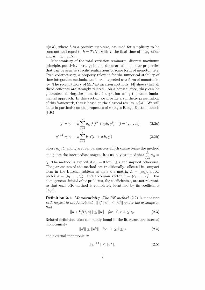
u(nh), where h is a positive step size, assumed for simplicity to beconstant and equal to h = T/Nt, with T the final time of integrationand n = 1, . . . , Nt.
Monotonicity of the total variation seminorm, discrete maximumprinciple, positivity or range boundedness are all nonlinear propertiesthat can be seen as specific realizations of some form of monotonicity.Even contractivity, a property relevant for the numerical stability oftime integration methods, can be reintepreted as a form of monotonic-ity. The recent theory of SSP integration methods [14] shows that allthese concepts are strongly related. As a consequence, they can beguaranteed during the numerical integration using the same funda-mental approach. In this section we provide a synthetic presentationof this framework, that is based on the classical results in [31]. We willfocus in particular on the properties of s-stages Runge-Kutta methods(RK)
gi = un + hs∑j=1
aij f(tn + cjh, gj) (i = 1, . . . , s) (2.2a)
un+1 = un + hs∑i=1
bi f(tn + cih, gi) (2.2b)
where aij , bi and ci are real parameters which characterize the method
and gi are the intermediate stages. It is usually assumed thats∑j=1
aij =
ci. The method is explicit if aij = 0 for j ≥ i and implicit otherwise.The parameters of the method are traditionally collected in compactform in the Butcher tableau as an s × s matrix A = (aij), a rowvector b = (b1, . . . , bs)
ᵀ and a column vector c = (c1, . . . , cs). Forhomogeneous initial value problems, the coefficients ci are not relevant,so that each RK method is completely identified by its coefficients(A, b).
Definition 2.1. Monotonicity. The RK method (2.2) is monotonewith respect to the functional ‖·‖ if ‖un‖ ≤ ‖u0‖ under the assumptionthat
‖u+ hf(t, u)‖ ≤ ‖u‖ for 0 < h ≤ τ0. (2.3)
Related definitions also commonly found in the literature are internalmonotonicity
‖gi‖ ≤ ‖un‖ for 1 ≤ i ≤ s (2.4)
and external monotonicity
‖un+1‖ ≤ ‖un‖. (2.5)
5
Assumption (2.3), commonly found in many references, see e.g. [9],[18], [20], [21], [26], [27], [29], [36] and [37], essentially amounts todefine τ0 as the maximum time step under which the explicit Eulermethod is monotone. In these studies the critical step size for mono-tonicity is determined such that property 2.1 is verified for all
0 < h ≤ c τ0 (2.6)
thus making the RK method conditionally monotone. If property 2.1 isverified for any step size h, then the method is called unconditionallymonotone. In assessing monotonicity of different RK methods, theinterest lies usually in determining the maximal step size coefficient csuch that a time integration method is conditionally monotone.
Frequently, the convex functional ‖·‖ is intended either as the supre-mum norm ‖x‖ = ‖x‖∞ = supi |xi| or as the total variation seminorm‖x‖ = ‖x‖TV =
∑i |xi+1 − xi|, where xi are the components of the
vector x. We remind that ‖x‖TV is a seminorm since it may vanish forx 6= 0 when xi = C. Numerical methods statisfying 2.1 under the to-tal variation seminorm are called total variation diminishing (TVD).They are especially important in the numerical solution of hyperbolicconservation laws, see e.g. [28], [33], [37].
For some classes of initial value problems, the properties of positiv-ity and range boundedness play important roles in obtaining physicallymeaningful numerical solutions. Furthermore, due to the strongly non-linear form of such problems, the ability in maintaining such nativeproperties also in the numerical solutions is important in order toguarantee numerical stability of time integrations.
Definition 2.2. Positivity. The RK method (2.2) is positive ifwhenever u0 ≥ 0 it guarantees that un+1 ≥ 0 under the assumptionthat
u+ hf(t, u) ≥ 0 for 0 < h ≤ τ0. (2.7)
Definition 2.3. Range boundedness. The RK method (2.2) isrange bounded in [χ, ψ] if whenever χ ≤ u0 ≤ ψ it guarantees thatχ ≤ un+1 ≤ ψ under the assumption that
χ ≤ u+ hf(t, u) ≤ ψ for 0 < h ≤ τ0. (2.8)
Both these properties are usually guaranteed if a time step limita-tion of the form (2.6) is respected. Even though these properties areformally different from the monotonicity property 2.1, they can beequally derived from monotonicity after proper assumptions on thefunction f . In this respect, the generalization of monotonicity toarbitrary sublinear functionals ‖·‖ becomes relevant. Following the
6
presentation in [25] and [39], it is useful to introduce two sublinearfunctional, denoted respectively as floor and ceil functional
‖u‖bχc = −minj
(χ, uj) (2.9a)
‖u‖dψe = maxj
(ψ, uj). (2.9b)
These functionals are not seminorms, since they both violate property‖λv‖ = |λ|‖v‖ for λ=−1. Using both functionals the range bound-edness property 2.3 naturally follows, while setting χ= 0 in the floorfunctional the positivity property 2.2 is recovered. As a consequence,by introducing the floor and ceil functionals it possible to recast Defi-nitions 2.2 and 2.3 in a form similar to Definition 2.1. Thus positivityand range boundedness can just be interpreted as different forms ofmonotonicity.
Alternatively, positivity and range boundedness can also be consid-ered as two alternative realizations of the discrete maximum principle.
Definition 2.4. Discrete Maximum Principle. The RK method(2.2) follows the discrete maximum principle if it guarantees that
minju0j ≤ un+1
j ≤ maxju0j
under the assumption that for 0 < h ≤ τ0 and ∀u ∈ Rm with compo-nents up
min1≤q≤m
uq ≤ up + τ0fp(t, u(t)) ≤ max1≤q≤m
uq, (1 ≤ p ≤ m). (2.10)
Similarly to the other properties, range boundedness may be verifiedunder a step size restriction analogous to (2.6). Again following [25]and [39], we introduce two relevant sublinear functionals, denoted asmax and min functional
‖u‖> = maxjuj (2.11a)
‖u‖< = −minjuj (2.11b)
which allow us to write the assumption (2.10) in the form (2.3). Byassuming the monotonicity property 2.1 under the functionals (2.11)the discrete maximum principle 2.4 directly follows.
Contractivity of numerical approximation methods has been ex-tensively studied. Relevant conclusions on step size conditions forcontractivity have been given in [38], while contractivity of RK fornonlinear problems was thoroughly examined in [31].
7

Definition 2.5. Contractivity. The RK method (2.2) is contractiveif ‖un+1 − un+1‖ ≤ ‖u0 − u0‖ under the assumption that
‖u− u+ h(f(t, u)− f(t, u))‖ ≤ ‖u− u‖ for 0 < h ≤ τ0. (2.12)
Usually, Definition 2.5 is verified under a step size restriction in theform of (2.6). For conditional contractivity, the circle condition thatwas originally assumed in [31] is
‖f(t, u)− f(t, u) + ρ(u− u)‖ ≤ ρ‖u− u‖ (2.13)
It was shown later in [20] that this condition can be considered as aspecial form of (2.3). See also [39] for additional considerations onthese issues.
In the framework introduced above, all these properties appear asdifferent forms of monotonicity under a proper choice of the convexfunctional ‖.‖. It is thus possible to extend the analytical results fromthe preservation of a specific property to that of any other relatedproperty. Every convex functional will be retained under convex com-binations of single RK methods preserving it. Even though in principlethis approach may not lead to sharp bounds, experience shows thatthe time step limits obtained from monotonicity are representative forthe preservation of the other properties as well [27]. The sharper re-sults obtained in the context of inner product norms [19], for example,did not lead to time step limits significantly different for the practicaluse of conditionally monotone RK methods. It is to be noticed thatRK methods that are non-monotone under arbitrary functionals mayindeed be conditionally monotone under inner product norms, as in[19]. For linear problems these conditions relax even further, see e.g.,[38], [42].
As a consequence, it appears useful to extend the contractivityresults to the other properties. To this purpose, the absolute mono-tonicity introduced in [31] allows to investigate necessary and sufficientconditions for contractivity of RKs in dissipative problems under sub-linear functionals, including the maximum norm. In [9] this approachwas extended to study monotonicity of general RK under arbitraryseminorms. One of the relevant results is that the maximal step sizecoefficient for monotonicity is equal to the maximal step size for con-tractivity. Recently these conclusions were extended to the analysisof general linear methods under arbitrary convex functionals in [39].
For our next discussion we will focus on irreducible RK methods,which are the only ones practically relevant. For a definition of irre-ducibility see [16]. Following [31], we introduce for real ξ the quantities
A(ξ) = A(I − ξA)−1, bᵀ(ξ) = bᵀ(I − ξA)−1,
e(ξ) = (I − ξA)−1e, ϕ(ξ) = 1 + ξbᵀ(I − ξ)A−1e.(2.14)
8

Definition 2.6. Absolute monotonicity of RK. An irreducible s-stage RK (A, b) is absolutely monotone at ξ ∈ R if A ≥ 0, b ≥ 0, e ≥ 0and ϕ ≥ 0 elementwise.
For the stability function ϕ, this entails that dkϕdzk
(ξ) ≥ 0 for any k ≥ 0,since the rationale behind Definition 2.6 lies in the Taylor expansion ofsome characteristic functions of a RK method, including the stabilityfunction. The quantities (2.14) form the coefficients of such expan-sions, see [22] and [31] for further details. These notations are usefulto introduce the radius of absolute monotonicity for a RK method.
Definition 2.7. Radius of absolute monotonicity. An s-stageRK with scheme (A, b) and A ≥ 0 and b ≥ 0 is characterized by itsradius of absolute monotonicity defined for all ξ in −r ≤ ξ ≤ 0 as
R(A, b) = sup{r :r ≥ 0,
A(ξ) ≥ 0, bᵀ(ξ) ≥ 0, e(ξ) ≥ 0, ϕ(ξ) ≥ 0}.(2.15)
In [31], two useful results are derived, that simplify the practical es-timation of the absolute monotonicity radius. We introduce the inci-dence matrix Inc(A) as the matrix containing 0 or 1 if the correspond-ing element in the matrix A is ai,j = 0 or ai,j 6= 0 respectively.
Theorem 2.1 ([31], Theorem 4.2). For an irreducible RK R(A, b) > 0iff A ≥ 0, b > 0 and Inc(A2) ≤ Inc(A).
Lemma 2.1 ([31], Lemma 4.4). For an irreducible RK R(A, b) ≥ riff A ≥ 0 and (A, b) is absolutely monotone at ξ = −r.
More compact definitions of the radius of absolute monotocity in-volve the use of matrices derived from the Butcher tableau, see e.g.,[30], but for the purpose of this work we found the use of the orig-inal definition more convenient. Other classical results for the prac-tical identification of RK properties from the corresponding Butchertableau stem from the stage order, that has practical relevance toavoid the order reduction phenomenon during stiff transients.
Theorem 2.2 ([31], Theorem 8.5). Any RK with A ≥ 0 has stageorder p ≤ 2. If p = 2 then A must have a zero row.
Lemma 2.2 ([31], Lemma 8.6). Any RK with b > 0 has stage orderp ≥ bp−1
2 c .
Theorem 2.3 ([31], Theorem 8.3). Unconditional contractivity.The order barrier for R(A, b) =∞ in a RK is p ≤ 1. Some first orderunconditionally contractive RKs are the implicit Euler, the RADAUIA and the RADAU IIA methods.
9

Theorem 2.4 ([31], Corollary 8.7). Conditional contractivity.The order barriers for R(A, b) ≥ 0 under the circle condition (2.13)are p ≤ 4 for explicit RK and p ≤ 6 for implicit RK.
As a consequence, step size restrictions on RK of formal order p >1 are inevitable to preserve contractivity of the numerical solution.The analysis was recently extended in [39] to a much larger class ofmethods, including IMEX methods (see also [22]). This implies thatthe order barriers above are inevitable for a very large class of timediscretization methods.
In recent literature [14], [15], methods satisfying condition (2.5)for a general convex functional are called strong-stability preserving(SSP), in order to specify their ability to preserve any convex func-tional bound. Thus they generalize classical TVD methods specificallydeveloped for hyperbolic conservation laws.
Definition 2.8. Strong stability preserving (SSP). The RK method(2.2) is SSP with respect to the functional ‖·‖ if ‖un‖ ≤ ‖u0‖ underthe assumption that
‖u+ hf(t, u)‖ ≤ ‖u‖ for 0 < h ≤ τ0. (2.16)
The SSP coefficient is the largest constant c ≥ 0 such that this defini-tion is verified for all 0 < h ≤ cτ0.
The definition above closely follows Definition 2.1 for monotonicity;indeed, these definitions are equivalent. The SSP coefficient c turnsout to be strongly related to the radius of absolute monotonicity in-troduced in Definition 2.7.
Theorem 2.5 ([10], Theorem 3.4). For an irreducible RK, c = R(A, b).
Recent studies focused on the search of SSP-optimal RK methods hav-ing large SSP coefficients. While explicit SSP RKs are known sincethe seminal work in [37], a search for implicit SSP RKs started onlyrecently in [11] and [30], where it was found that the SSP-optimalimplicit RKs of order p = 2 and p = 3 are indeed SDIRK, whilethe optimal methods for p = 4 are DIRK. In the quest for improvedmonotonicity, the classes of two-step RKs [29] and diagonally split RK[2], [3], [34] have been investigated in the literature, with mixed suc-cess. Starting from the framework introduced above in our followinganalysis we will consider all these properties just as specific realiza-tions of absolute monotonicity. As a consequence, in the next sectionsthey will be briefly referred to as monotonicity of the time integrationmethods.
10

3 Strong stability preservation for the
TR-BDF2 method
We analyze here the monotonicity properties of the TR-BDF2 method,originally introduced in [1] and successively studied in [24] as a DIRK.The same method was rediscovered in [6] and has been applied alsoin [13] to treat the implicit terms in an additive Runge-Kutta (ARK).A semi-implicit, semi-Lagrangian reinterpretation of this method hasrecently been proposed in [41].
We rely on the monotonicity and contractivity results reviewed inSection 2. In its original formulation, TR-BDF2 is defined as a one-step method resulting from the composition of the trapezoidal rule inthe first substep, followed by BDF2 in the second substep. This com-bination is empirically justified under the rationale of combining thegood accuracy of the trapezoidal rule with the stability and dampingof fast modes guaranteed by BDF2. The TR-BDF2 method is
un+γ − γ
2hfn+γ = un +
γ
2hfn (3.1a)
un+1 − (1− γ)
(2− γ)hfn+1 =
1
γ(2− γ)un+γ − (1− γ)2
γ(2− γ)un (3.1b)
where γ ∈ (0, 1) is a parameter whose value determines the stabilityand monotonicity properties of the method. By requiring that bothstages have the same Jacobian, the value γ = 2−
√2 was derived in [1].
This value is also the only one for which the method (3.1) is L-stable.As outlined in [24], the TR-BDF2 method can be rewritten as a DIRKmethod. However, instead of closely following this reference, we willfirst derive the DIRK family associated to (3.1) before imposing thecondition on the Jacobian. The Butcher tableau for this DIRK familyis then
0 0
γ γ2
γ2
1 12(2−γ)
12(2−γ)
1−γ2−γ
12(2−γ)
12(2−γ)
1−γ2−γ
We remark that, by imposing the condition a22 = a33, the optimalvalue for γ able to guarantee L-stability is readily obtained. Thestability function associated to the above DIRK family is
ϕ(ξ) =det(I − ξA+ ξebᵀ)
det(I − ξA)=
[1 + (1− γ)2]ξ + 2(2− γ)
2(2− γ)(1− ξ γ2 )(1− ξ 1−γ2−γ )
. (3.2)
11
The rational polynomial defining the stability function of the DIRKfamily has a single zero at ξ = 2(γ−2)
1+(1−γ)2, which is always negative
for all possible values of parameter γ, and two poles at ξ = 2γ and
ξ = 2−γ1−γ respectively, which are always positive. While in [1] it is
argued that there is a double pole at ξ = 2γ , this is true only for the
numerical value of γ satisfying a22 = a33. As shown in [24], the TR-BDF2 method is embedded in a (2,3) Runge-Kutta pair, thus allowingan efficient estimation of the time discretization error, in case step sizeadaptation is required. Additionally, it is immediate to find out thatthe stage order of TR-BDF2 is indeed p=2, thus making the methodresilient to order reduction in stiff problems (see e.g., [18], [34]).
We analyze the monotonicity properties of the DIRK family gen-eralizing the TR-BDF2 by following [9], [10], [31]. Following the defi-nition (2.15), we find
A(ξ) =
0 0 0γ2
1− γ2ξ
γ2
1− γ2ξ
0
12(2−γ)(1− γ
2ξ)β
12(2−γ)(1− γ
2ξ)β
1−γ(2−γ)β
bᵀ(ξ) =
β−ξγ/22(2−γ)
β−ξγ/22(2−γ)
(1−γ)β2−γ
e(ξ) =
1
1+ γ2ξ
1− γ2ξ
[1+(1−γ)2]ξ+2(2−γ)2(2−γ)(1−ξ γ
2)β
ϕ(ξ) =
[1 + (1− γ)2]ξ + 2(2− γ)
2(2− γ)(1− ξ γ2 )β
where we have set β=1−ξ(1−γ)/(2−γ). The main conclusion is that
the radius of absolute monotonicity of TR-BDF2 is R(A, b)= 2(2−γ)1+(1−γ)2
and that it is maximized for γ=2−√
2, which is exactly the value thatmakes the DIRK family L-stable. With this value of the parameterγ, the absolute monotonicity radius is R(A, b)≈ 2.414. From [9], weconclude that this is also the step size coefficient c for conditionalmonotonicity of the method under arbitrary seminorms and sublinearfunctionals for any nonlinear problem.
4 Two unconditionally monotone vari-
ants of TR-BDF2
The results reviewed in Section 2 lead to the conclusion that there areno unconditionally monotone RK methods of order higher than one.
12

For stiff initial value problems, this implies that even implicit higherorder RK methods will be always subject to a CFL-like condition formonotonicity. Thus, the only RK method that does not need to com-ply with a time step restriction and that can be safely used withouttime step adaption is in practice the implicit Euler method. Due tosuch limitation, which is particularly relevant for problems with chem-ical kinetics, some solution methods found in literature rely exclusivelyon it, sacrificing accuracy for improving stability and consistency [44].
We propose here two hybridization strategies of TR-BDF2 withthe implicit Euler method, that can be activated using a sensor de-tecting violations of relevant functional bounds. These hybrid schemesbring time integration back to a first order unconditionally monotonemethod whenever the sensor detects a violation of a selected func-tional bound during the current integration. Empirically, this localloss in accuracy should not be too detrimental on solution accuracyif time step is not too large. Our proposed methods apply this safemode whenever it is expected from SSP theory that TR-BDF2 mayproduce non-monotone solutions.
The hybrid TR-BDF2 method is thus obtained by introducinga weighting parameter α ∈ [0, 1] in both stages of TR-BDF2
un+γ − γh(1− α
2)fn+γ = un + γh
α
2fn (4.1a)
un+1 − (1− γ)h
α(1− γ) + 1fn+1 =
=α( 1
γ − 1) + 1
α(1− γ) + 1un+γ − α
α(1− γ) + 1
(1− γ)2
γun. (4.1b)
For α = 1 the first step is the trapezoidal rule and the second step isthe BDF2 formula, thus reconstructing the original TR-BDF2 (3.1).For α = 0 each of the two steps above is equivalent to an implicitEuler step, thus transforming the hybrid TR-BDF2 in succession oftwo substeps of the implicit Euler method (IE-IE) of length γh and (1−γ)h, respectively, and making the method unconditionally monotone.
The hybrid TR-BDF2 method can be rewritten as a DIRK schemeas done for (3.1). By injecting the first step in the second one, theButcher tableau of the hybrid TR-BDF2 method is found
0 0
γ γ α2 γ(1− α
2
)1 α
2α(1−γ)+γα(1−γ)+1
(1− α
2
) α(1−γ)+γα(1−γ)+1
1−γα(1−γ)+1
α2α(1−γ)+γα(1−γ)+1
(1− α
2
) α(1−γ)+γα(1−γ)+1
1−γα(1−γ)+1
13

For the unconditionally monotone method (α = 0), equivalent to adouble step of implicit Euler, the above above reduces to
0 0
γ 0 γ
1 0 γ 1− γ
0 γ 1− γ
The stability function of the DIRK family associated to the hybridTR-BDF2 method is thus
ϕ(ξ) =1 +
[α(1−γ)+γα(1−γ)+1 − γ
(1− α
2
)]ξ
1−[
1−γα(1−γ)+1 + γ
(1− α
2
)]ξ + γ
(1− α
2
) 1−γα(1−γ)+1ξ
2(4.2)
From this expression for the case α = 1 we recover the stability func-tion (3.2) and for the unconditionally monotone case α = 0 the sta-bility function ϕ(ξ) = 1/[1− ξ + γ(1− γ)ξ2].
The DIRK family corresponding to the hybrid TR-BDF2 methodis thus entirely L-stable for every value of the parameter α, as evidentfrom Figure 1. Additonally for α=1 the value γ=2−
√2 correspond-
ing to TR-BDF2 maximizes the radius of absolute monotonicity, whilefor γ=2−
√2 starting from α=1 (TR-BDF2) the radius of absolute
monotonicity is progressively increased by decreasing α, while the or-der is reduced to p= 1 for α 6= 1, as evident from the absolute error|ϕ(z)−ez| in the asymptotic range (Re→0−, Im→0) in Figure 1. For-mally, we have limα→0R(A, b)=∞, thus recovering the unconditionalmonotonicity of the implicit Euler method.
The hybrid TR-BDF2 method can be exploited through differentstrategies, since by choosing values of the parameter 0 ≤ α ≤ 1 itis possible to produce a continuous blend of the two main schemesvarying the radius of absolute monotonicity accordingly. In our workwe adopt a simpler approach and we investigate two alternative modesfor enforcing monotonicity under the selected step size.
4.1 TR-BDF2 blended
In the hybrid in time mode the strategy is to switch from the de-fault α= 1 (TR-BDF2) to the unconditionally monotone mode α= 0(IE-IE) whenever a suitable sensor detects a violation of some globalfunctional bound on TR-BDF2 solution. After each detected violationby the TR-BDF2 solution, the time step integration is repeated in IE-IE mode. We call this simple method TR-BDF2 blended, since
14

(a) (b)
(c) (d)
Figure 1: Hybrid TR-BDF2 in comparison with implicit Euler: a) stabilityfunctions along the negative real axis, b) modulus of the stability functionsalong the imaginary axis, c) absolute error functions along the negative realaxis showing the asymptotic and non-asymptotic ranges, d) absolute errorfunctions along the positive imaginary axis.
(a) (b)
Figure 2: Stability regions (outside portions of the plane): a) stability bound-aries for the hybrid TR-BDF2 and the implicit Euler methods, b) stabilityregion of the additive Runge-Kutta corresponding to the TR-BDF2 parti-tioned method.
15

it provides automatic adaption of the α value by enforcing uncondi-tional monotonicity only during critical transients. To this purposewe introduce the global sensor function
σ = sg(un+1) =
{1 if ‖un+1‖ ≤M0 otherwise.
(4.3)
that is able to determine if the generic functional bound M on ‖·‖is violated by the numerical solution un+1. For each time step thealgorithm of TR-BDF2 blended with γ=2−
√2 is:
1. Set α = 1 and perform the current integration by (4.1) to findthe tentative solution u∗.
2. Apply the sensor σ = sg(u∗).
• If σ=1, set un+1 = u∗ and go to the next time step.
• If σ= 0, set α = σ, repeat the current integration by (4.1)to find the solution un+1 and go to the next time step.
This basic method is A-stable, L-stable and unconditionally mono-tone.
4.2 TR-BDF2 partitioned
In the hybrid in solution space mode the switch from the default TR-BDF2 to the unconditionally monotone IE-IE mode is applied onlyfor those solution components which are likely to produce violationsof a relevant property under the assigned time step size. In orderto detect this behaviour we rely on SSP theory results by applyingDefinition 2.1 together with the computed value of R(A, b)≈2.414 forTR-BDF2. Since this strategy exploits locality, we introduce the localsensor function
σi = sl(un+1i ) =
{1 if ‖un+1
i ‖ ≤Mi
0 otherwise.(4.4)
that detects any componentwise violation of the functional bound Mi
on ‖·‖. In particular for each time step the algorithm is:
1. Perform a tentative step of forward Euler
u∗ = un + hEE f(tn, un)
using a monotonicity-scaled time step hEE = h/R(A, b).
2. Apply the sensor σi = sl(u∗i ) (i = 1, . . . ,m) on the tentative
solution to construct the partitioning matrix S=diag{σi}.
16
3. Identifying with aij and bi the coefficients corresponding to thetableau for α = 1 and with aij and bi the coefficients for α= 0in (4.1), construct the automatically partitioned RK method
gi = un + hs∑j=1
[ aijS + aij(I − S) ] f(tn + cjh, gj) (4.5a)
un+1 = un + hs∑i=1
[ biS + bi(I − S) ] f(tn + cih, gi) (4.5b)
to find the solution un+1 from stage values gi (i=1, . . . , s) withγ=2−
√2.
Thus we have effectively transformed the hybrid TR-BDF2 (4.1) intoa partitioned Runge-Kutta method, in which the solution space isautomatically sorted into monotone and non-monotone componentsby performing a tentative forward Euler step on a suitably scaled timestep. It may also be interpreted as an additive Runge-Kutta method(see, e.g., [23]) from which the usual ARK stability region ϕ(z, w) =1 + (iwbᵀ + zbᵀ)(I − iwA− zA)−1e for the scalar test problem u′(t)=λu(t) + iµu(t) with u(0) =u0 is represented in Figure 2. In this casethe unconditionally monotone component z is computed by the IE-IEmethod while the conditionally monotone component w is integratedusing the original TR-BDF2. We call this second strategy TR-BDF2partitioned. It introduces a small overhead in computational timesince it always performs an explicit tentative step, even in case of asuccessful integration from TR-BDF2. Clearly, the overall order ofaccuracy for both strategies will be limited to p = 1 whenever thesensor functions are activated in the current time step and similarlyfor the stage order p, but both strategies preserve L-stability and donot spoil the linearity of the base methods, they also preserve anylinear invariant and as such they allow atomic mass conservation (see,e.g., [35]).
5 Potential competitors of TR-BDF2
In order to compare the properties of TR-BDF2 to those of othersimilar methods in numerical test problems, we introduce here somesecond order methods with similar characteristics. We will make ourassessment by comparing the performance of TR-BDF2 and its twohybrid variants from Section 4 against the following methods as wellas against other classic methods, such as implicit Euler (R(A, b) =∞)and Crank-Nicolson (R(A, b) = 2).
17

5.1 SSP-optimal SDIRK 2(2)
The 2-stage SSP-optimal Runge-Kutta method of second order, namelythe second order RK with the largest radius of absolute monotonicity,was discovered in [11]. Later it was confirmed in [30] to be also theoptimal 2-stage second order implicit RK through extensive numericalsearch. The Butcher tableau of DIRK 2(2) is
14
14
34
12
14
12
12
As apparent from the tableau, this method consist of two consecutiveapplications of the implicit midpoint rule, that is characterized byR(A, b) = 2, exactly as the Crank-Nicolson method. As a consequencethe radius of absolute monotonicity of the SSP-optimal SDIRK 2(2)is R(A, b) = 4. Moreover the method inherits all the properties of theimplicit midpoint rule, being A-stable and symplectic, but it is notL-stable as TR-BDF2.
5.2 ROS2
Among the potential competitors of TR-BDF2 we also include theRosenbrock method proposed in [8] and later applied in atmosphericchemistry problems, see e.g. [35], [45]. The Butcher tableau is
0 0 γ
1 1 0 −2γ γ
12
12
with γ = 1 + 1√2. In addition to L-stability, from numerical experi-
ments in [45] it was found that it also has interesting positivity prop-erties. This was empirically justified by observing that the stabilityfunction is positive along the entire negative real axis. In [35] thisobservation was extended to the first two derivatives of the stabilityfunction. However, from the framework in Section 2 it turns out thatR(A, b)= 0, since the third derivative of the stability function is nega-tive along the negative portion of the real axis. In spite of this, the factthat up to the second derivative we have positivity for any negativereal value can be interpreted as a sort of weak absolute monotonic-ity. Even though small violations of arbitrary functionals cannot be apriori excluded at any step size, from numerical experiments in Sec-tion 6 we found an intrinsic resiliency against violations of the TVDproperty, even from initial conditions of limited regularity.
18

5.3 Modified Patankar Runge-Kutta
A suitable second order method for stiff chemical problems is the Mod-ified Patankar Runge-Kutta (MPRK) introduced in [5] and later ex-tended to third order accuracy in [12]. The MPRK method achievesunconditional positivity through proper weighting of production and
destruction terms and it conserves the quantitym∑j=1
uj , which repre-
sents the total mass of the system if species are expressed as massconcentrations.However, the mass of the atomic species is not con-served. Additionally, due to the specific form required to the righthand side, it can be used in a PDE framework only by introducing asource term splitting.
6 Numerical experiments
A number of numerical experiments have been carried out, in orderto assess the performance of the TR-BDF2 method and its hybridvariants introduced in Section 4 against the other methods describedin Section 5. The range of the test cases covers a reactive zero di-mensional test problem, here adapted to the MPRK method, a onedimensional advection problem, an advection diffusion reaction prob-lem for a mixture of chemical species, as well as two typical nonlinearconservation laws. For PDE tests, we have considered discontinousinitial conditions, in order to show the emergence of critical issues formonotonicity. This provides the most stringent test, as we experi-enced from other computations, not reported here, using more regularinitial conditions. In all test cases the nonlinear system associated toimplicit RKs was solved using MATLAB’s fsolve with a tolerance oftol = 10−10, except when otherwise stated. All computations wereperformed on a single Intelr CoreTMi5-2540M (2.60 GHz) on a laptopwith 4 GB RAM running Linux kernel 3.13.0-24-generic. We dotnot claim that the error-workload curves reported here are immedi-ately relevant for the selection of step sizes or numerical methods, butwe consider them as representative of the relative workload expectedfrom the methods assessed.
6.1 0-D chemical model problem: the Brusse-lator
As a first tes,t we use a typical nonlinear chemical kinetics prob-lem. The same issues are shared by all chemistry modelling problems,which require positivity for each solution component. Consequently,
19

we adopt both hybridization strategies from Section 4 with global andlocal positivity sensors built from the floor norm (2.9) with χ = 0. Inthe zero dimensional chemical model problem we measure the maxi-mum error during time integrations from the l∞-time absolute errornorm for the i-th species
‖ei‖∞ = maxn=1,...,Nt
|uni − uni | (6.1)
where Nt is the number of time steps, uni is the solution in the n-th time step and uni is the reference solution at the same time stepobtained with MATLAB ode15s using absolute and relative error tol-erance levels of AbsTol=10−14 and RelTol=10−13 respectively. In ournumerical results we will refer to the error on species i= 1, which isassumed to be representative of the problem.
We consider thus the original Brusselator system in [32]:
u′1 = −k1u1 (6.2a)
u′2 = −k2u2u5 (6.2b)
u′3 = k2u2u5 (6.2c)
u′4 = k4u5 (6.2d)
u′5 = k1u1 − k2u2u5 + k3u25u6 − k4u5 (6.2e)
u′6 = k2u2u5 − k3u25u6 (6.2f)
since this form allows to write the right hand side in a form suitableto MPRK. In particular we follow the procedure in [12], which in thiscase can be applied, since the stoichiometric matrix has proper rank([12], Assumption 2.1). We solve this problem for 0 ≤ t ≤ 10 assumingk1 = k2 = k3 = k4 = k5 = k6 = 1 as in the reduced model and startingfrom the initial condition u1 =u2 = 10, u3 =u4 = 0 and u5 =u6 = 0.1.The results in Figure 3 show that Crank-Nicolson, SDIRK 2(2) andTR-BDF2 (clipped to avoid negative values) are almost equivalentin performance, with a slight advantage for the SSP-optimal SDIRK.MPRK shows similar accuracy at same step sizes, while it outperformsall the other methods in terms of workload, being it the only explicitmethod. ROS2 offers intermediate performance. Blended and parti-tioned TR-BDF2 are here equivalent to the clipped version, due tolimited size of the integration interval T . Similar results, not shownhere, were obtained for the simple geobiochemical problem from [5].Even though the results from MPRK are promising, in the next testswe are forced to abandon it, since it would require a source splittingto the advection diffusion reaction problem that is out of our scope.
20
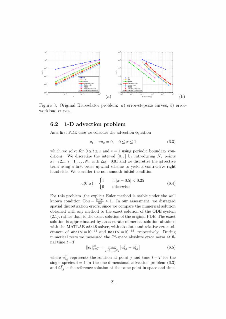
(a) (b)
Figure 3: Original Brusselator problem: a) error-stepsize curves, b) error-workload curves.
6.2 1-D advection problem
As a first PDE case we consider the advection equation
ut + vux = 0, 0 ≤ x ≤ 1 (6.3)
which we solve for 0≤ t≤ 1 and v = 1 using periodic boundary con-ditions. We discretize the interval (0, 1] by introducing Nx pointsxi= i∆x, i=1, . . . , Nx with ∆x=0.01 and we discretize the advectiveterm using a first order upwind scheme to yield a contractive righthand side. We consider the non smooth initial condition
u(0, x) =
{1 if |x− 0.5| < 0.25
0 otherwise.(6.4)
For this problem ,the explicit Euler method is stable under the wellknown condition Cou = |a|∆t
∆x ≤ 1. In our assessment, we disregardspatial discretization errors, since we compare the numerical solutionobtained with any method to the exact solution of the ODE system(2.1), rather than to the exact solution of the original PDE. The exactsolution is approximated by an accurate numerical solution obtainedwith the MATLAB ode45 solver, with absolute and relative error tol-erances of AbsTol=10−14 and RelTol=10−13, respectively. Duringnumerical tests we measured the l∞-space absolute error norm at fi-nal time t=T
‖ei‖∞t=T = maxj=1,...,Nx
∣∣uTi,j − uTi,j∣∣ (6.5)
where uTi,j represents the solution at point j and time t = T for thesingle species i = 1 in the one-dimensional advection problem (6.3)and uTi,j is the reference solution at the same point in space and time.
21
Furthermore, in order to assess any violation of the TVD property, wemonitored also the TV -space l∞-time seminorm for species i
‖TVi‖∞ = maxn=1,...,Nt
Nx∑j=1
∣∣uni,j+1 − uni,j∣∣ . (6.6)
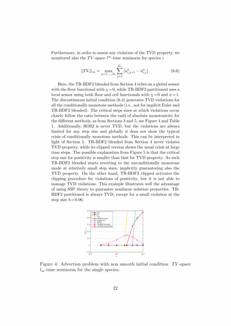
Here, the TR-BDF2 blended from Section 4 relies on a global sensorwith the floor functional with χ=0, while TR-BDF2 partitioned uses alocal sensor using both floor and ceil functionals with χ=0 and ψ=1.The discontinuous initial condition (6.4) generates TVD violations forall the conditionally monotone methods (i.e., not for implicit Euler andTR-BDF2 blended). The critical steps sizes at which violations occurclosely follow the ratio between the radii of absolute monotonicity forthe different methods, as from Sections 3 and 5, see Figure 4 and Table1. Additionally, ROS2 is never TVD, but the violations are alwayslimited for any step size and globally it does not show the typicalcrisis of conditionally monotone methods. This can be interpreted inlight of Section 5. TR-BDF2 blended from Section 4 never violatesTVD property, while its clipped version shows the usual crisis at largetime steps. The possible explanation from Figure 5 is that the criticalstep size for positivity is smaller than that for TVD property. As suchTR-BDF2 blended starts reverting to the unconditionally monotonemode at relatively small step sizes, implicitly guaranteeing also theTVD property. On the other hand, TR-BDF2 clipped activates theclipping procedure for violations of positivity, but it is not able tomanage TVD violations. This example illustrates well the advantageof using SSP theory to guarantee nonlinear solution properties. TR-BDF2 partitioned is always TVD, except for a small violation at thestep size h=0.06.
Figure 4: Advection problem with non smooth initial condition: TV -spacel∞-time seminorm for the single species.
22

(a) (b)
Figure 5: Advection problem with non smooth initial condition: a) error-stepsize curves, b) error-workload curves.
The accuracy results in Figure 5 maintain the consistent rankingfrom the zero dimensional problem. ROS2 now features a non uni-form convergence and it achieves higher accuracy for 0.01<h < 0.04by sacrificing monotonicity, as evident when comparing Figures 4 and5. TR-BDF2 blended shows a degradation in accuracy at larger stepsizes, due to the intervention of the IE-IE mode triggered by the pos-itivity monitor, also evidenced from the order reduction. The TR-BDF2 partitioned is the only method able to obtain tighter accuracylevels similar to SDIRK 2(2), while additionally mantaining the TVDproperty with the exception of one step size. When repeating the sameadvection test with a smooth initial condition, the results obtained,not shown here, are similar to those in the chemical model problemand they do not exhibit the order reduction and TVD violations re-ported above.
6.3 1-D advection diffusion reaction problem
As a representative case for chemical transport of reacting species weintroduce the advection diffusion reaction problem of three species
ut + vux = Duxx + f(u), 0 ≤ x ≤ 1. (6.7)
with periodic boundary conditions. Here u = [u1, u2, u3]T and D =diag{dii} is the diffusivity matrix. The nonlinear source term f(u) istaken from the simple geobiochemical model in [5]
f(u)1 = − u1u2
u1 + 1(6.8a)
f(u)2 =u1u2
u1 + 1− ku2 (6.8b)
f(u)3 = ku2 (6.8c)
23
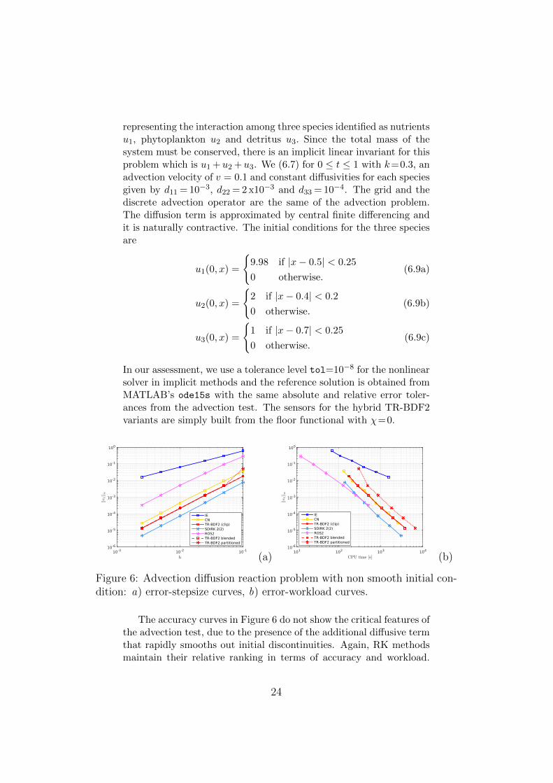
representing the interaction among three species identified as nutrientsu1, phytoplankton u2 and detritus u3. Since the total mass of thesystem must be conserved, there is an implicit linear invariant for thisproblem which is u1 +u2 +u3. We (6.7) for 0 ≤ t ≤ 1 with k=0.3, anadvection velocity of v = 0.1 and constant diffusivities for each speciesgiven by d11 = 10−3, d22 = 2 x10⁻³ and d33 = 10−4. The grid and thediscrete advection operator are the same of the advection problem.The diffusion term is approximated by central finite differencing andit is naturally contractive. The initial conditions for the three speciesare
u1(0, x) =
{9.98 if |x− 0.5| < 0.25
0 otherwise.(6.9a)
u2(0, x) =
{2 if |x− 0.4| < 0.2
0 otherwise.(6.9b)
u3(0, x) =
{1 if |x− 0.7| < 0.25
0 otherwise.(6.9c)
In our assessment, we use a tolerance level tol=10−8 for the nonlinearsolver in implicit methods and the reference solution is obtained fromMATLAB’s ode15s with the same absolute and relative error toler-ances from the advection test. The sensors for the hybrid TR-BDF2variants are simply built from the floor functional with χ=0.
(a) (b)
Figure 6: Advection diffusion reaction problem with non smooth initial con-dition: a) error-stepsize curves, b) error-workload curves.
The accuracy curves in Figure 6 do not show the critical features ofthe advection test, due to the presence of the additional diffusive termthat rapidly smooths out initial discontinuities. Again, RK methodsmaintain their relative ranking in terms of accuracy and workload.
24

TR-BDF2 clipped and the blended variant are almost indistinguish-able, while the partitioned version features slightly larger computa-tional times due to the partitioning step.
Figure 7: Advection diffusion reaction problem with non smooth initial con-dition: a) solution for u1(t = T ) when using h = 0.100, b) close-up in theregion of positity violation from ROS2.
A sample solution for this problem is shown in Figure 7, wherea close-up shows the typical positivity violation on u1 from ROS2.Violations of the TVD property are reported in Figure 8 where it isevident that all the methods are TVD, with the exceptions of Crank-Nicolson for h = 0.100 and ROS2 that is never TVD nor positivitypreserving.
Figure 8: Advection diffusion reaction problem with non smooth initial con-dition: TV -space l∞-time seminorm for the species u1.
6.4 1-D conservation laws
We complete our assessment by considering two well known hyperbolicconservation laws, see e.g. [33] for a more detailed discussion. The
25

first is the Burgers equation
ut = −f(u)x = −(
1
2u2
)x
, 0 ≤ x ≤ 1. (6.10)
which we solve for 0 ≤ t ≤ 1 with the smooth initial condition
u(0, x) =1
2+
1
4sin(2πx). (6.11)
The second is the Buckley-Leverett equation
ut = −f(u)x = −
(u2
u2 + 13(1− u)2
)x
, 0 ≤ x ≤ 1. (6.12)
which we solve for 0 ≤ t ≤ 18 with the discontinuous initial condition
u(0, x) =
{12 if x ≤ 0.5
0 otherwise.(6.13)
Both equations are here solved with periodic boundary conditions anddiscretized by a high resolution finite volume method using flux lim-iters, see e.g. [28], [33]. More specifically, for the Burgers equation weadopt the van Leer limiter
Ψ(θ) =θ + |θ|1 + |θ|
(6.14)
while for the Buckley-Leverett equation we select the Koren limiter
Ψ(θ) = max
{0 ; min
{2 ;
2
3+
1
3θ ; 2θ
}}. (6.15)
Due to the flux limiters, strictly speaking the the Jacobian is notdefined. Rather than approximating it by a finite difference discreti-zation, we again exclude ROS2 from our assessment, since it is knowna priori that it performs poorly on hyperbolic conservation laws.
In the numerical tests, we measured the l∞ norm in space (6.5)as well as the TV seminorm in space (6.6). The reference numericalsolution is obtained here by the MATLAB solver ode45 using againAbsTol=10−14 and RelTol=10−13, while the implicit stages of theRK methods are solved with a tolerance level of tol=10−10. Whilethe TR-BDF2 blended exploits a global sensor for the TV seminorm,the TR-BDF2 partitioned relies on a local sensor for the floor andceil functionals (2.9) with χ = 0.25 and ψ = 0.75 for the Burgersequation and χ = 0 and ψ = 0.5 for the Buckley-Leverett equation,respectively. These choices follows from the initial conditions (6.11)
26

and (6.13). Even though this local sensor is not properly a detectorof TVD violations, we use it as an approximate TV sensor due to theknown solution dynamics. This is not entirely correct, as we will seefrom the tests, but it comes from the difficulty of using a local test fora global property as TVD.
(a) (b)
Figure 9: Burgers equation with van Leer limiter and smooth initial condi-tion: a) solution at final time t = 1 when using h = 0.1, b) TV -space l∞-timeseminorm.
In Figure 9 we report the solution at the final time step for thecoarsest step size h= 0.1, corresponding to about Cou= 7.5. Whileimplicit Euler is able to maintain the TVD property with a strongsmoothing of the developing leading shock, all conditionally mono-tone methods develop visible oscillations downstream of this region. Inparticular, TR-BDF2 (here positive clipping is never activated) showsminor amplitudes with respect to SDIRK 2(2) and Crank-Nicolson.TR-BDF2 blended obtains a smoothed solution after several integra-tions in IE-IE mode. TR-BDF2 partitioned is qualitatively very closeto the reference solution with the best approximation for the shockamplitude, but it features also a reduction in the propagation speed,probably due to the smoothing of the imaginary parts for the pointsintegrated in IE-IE mode (see Figure 1). Significantly, both variantsalways remain TVD, even at Cou = 7.5. The other methods showTVD violations with the usual critical step size progression, see Fig-ure 9. The accuracy results for the Burgers equation are reported inFigure 10. Interesting behaviour appears at coarse stepsizes whereall the methods collapse about at the same accuracy of implicit Eu-ler. TR-BDF2 blended realizes a smooth adaption from the monotoneimplicit Euler accuracy to the TR-BDF2 asymptotic curve. It pre-serves always monotonicity, while Crank-Nicolson, SDIRK 2(2) andTR-BDF2 clipped violate it, as evident from Figure 9. The errorcurves from TR-BDF2 partitioned follows tha same behaviour even
27

though the l∞ error norm is penalized from the behaviour at the lead-ing shock.
(a) (b)
Figure 10: Burgers equation with van Leer limiter and smooth initial condi-tion: a) error-stepsize curves, b) error-workload curves.
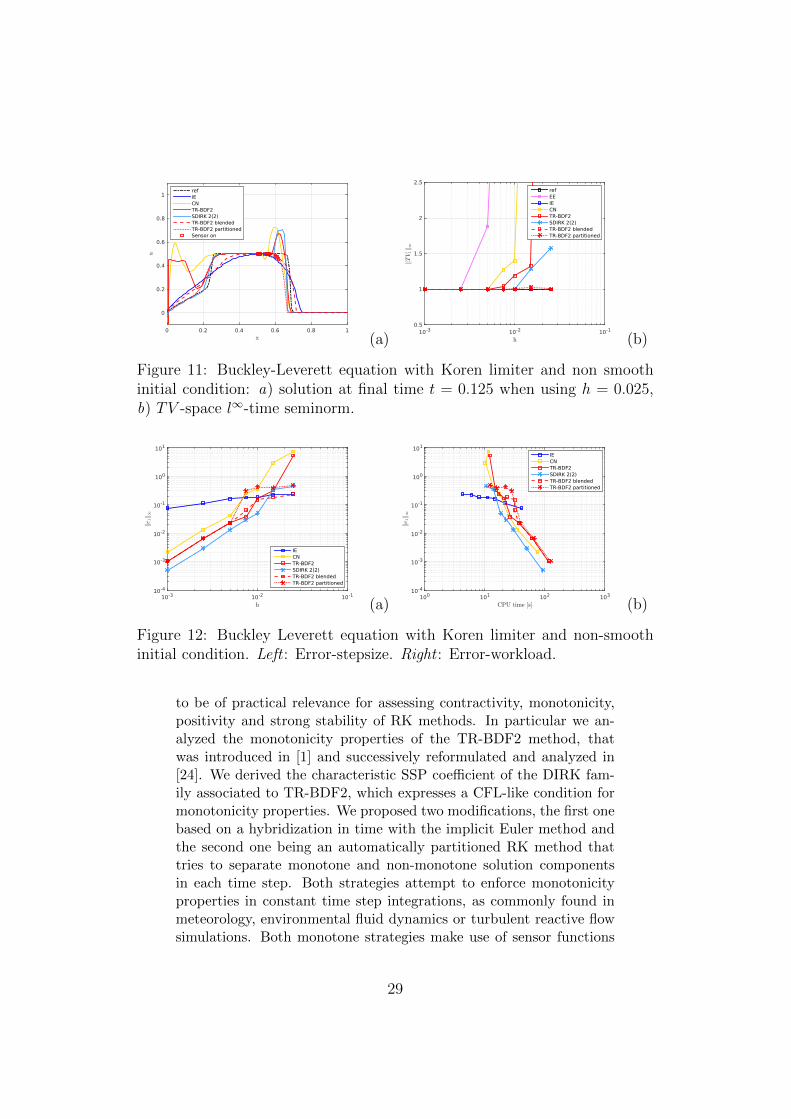
The Buckley-Leverett test provides a more stringest test due toits non-convex flux function. The solution at the final time step forthe step size h= 0.025 is shown in Figure 11. Again all conditionallymonotone methods develop oscillation on the trailing shock, while onlySDIRK 2 (2) develops a stable rarefaction wave, where Crank-Nicolsonand TR-BDF2 (again without clipping) develop additional waves. Im-plicit Euler and TR-BDF2 blended feature a strongly smoothed be-haviour, while TR-BDF2 partitioned remains free of oscillations dueto the activation of the local sensor that allows to develop the shockand rarefaction waves. Anyway it shows a reduction in the shockspeed, similarly as in the Burgers test, and some lmited violations ofthe TVD property at the largest step sizes, see Figure 11.
The accuracy curves for the Buckley-Leverett equation in Figure12 confirm our previous findings. Conditionally monotone methodsachieve worse results than implicit Euler at coarse step sizes, dueto the impact of the relevant TVD violations. TR-BDF2 blendedoffers a seamless compromise between accuracy at fine time steps andmonotonicity at coarse time steps, while TR-BDF2 partitioned obtainsqualitatively very good solutions, but it is penalized in the l∞ normby the wrong prediction on the advection speed of the leading shock.
7 Conclusions
We have reviewed a general framework for the preservation of somerelevant solution properties during numerical integrations with RKmethods. The generality of the absolute monotonicity results proved
28
(a) (b)
Figure 11: Buckley-Leverett equation with Koren limiter and non smoothinitial condition: a) solution at final time t = 0.125 when using h = 0.025,b) TV -space l∞-time seminorm.
(a) (b)
Figure 12: Buckley Leverett equation with Koren limiter and non-smoothinitial condition. Left : Error-stepsize. Right : Error-workload.
to be of practical relevance for assessing contractivity, monotonicity,positivity and strong stability of RK methods. In particular we an-alyzed the monotonicity properties of the TR-BDF2 method, thatwas introduced in [1] and successively reformulated and analyzed in[24]. We derived the characteristic SSP coefficient of the DIRK fam-ily associated to TR-BDF2, which expresses a CFL-like condition formonotonicity properties. We proposed two modifications, the first onebased on a hybridization in time with the implicit Euler method andthe second one being an automatically partitioned RK method thattries to separate monotone and non-monotone solution componentsin each time step. Both strategies attempt to enforce monotonicityproperties in constant time step integrations, as commonly found inmeteorology, environmental fluid dynamics or turbulent reactive flowsimulations. Both monotone strategies make use of sensor functions
29

able to detect local or global violations of suitable functional bounds,thus triggering a robust integration procedure when necessary to main-tain monotonicity. In this way accuracy, is sacrificed locally in orderto preserve monotonicity independently of the time step and stiffnessof the problem.
Both strategies were assessed empirically against other RK meth-ods on a series of benchmark problems, ranging from zero dimensionalchemical rectors to advection diffusion reaction equations and nonlin-ear conservation laws. The results show that the time hybridizationstrategies are able to guarantee a seamless compromise between ac-curacy at fine step sizes and monotonicity at coarse step sizes, whilethe partitioned strategy obtains promising results penalized only bya reduced shock advection speed at high CFL. Further research maybe useful to identify more appropriate sensors for triggering the parti-tioning method, as well as to extend the two strategies to SSP-optimalRK methods such as SDIRK 2(2).
8 Appendix
8.1 Relevant properties for chemical kineticsproblems
Ordinary differential equations in the form (2.1) arise in the contextof chemical kinetics when the reaction term is modeled by the massaction law. By ignoring the presence of additional terms in advection-diffusion-reaction PDEs, we briefly review here the reaction term.
Considering a chemical system having Ns species interacting in Nr
chemical reactionsNs∑q=1
lpquqkp−→
NS∑q=1
rpquq
the evolution of the molar concentrations is described by the massaction law:
d
dtu(t) = ω and t ≥ t0, (8.1a)
u(t0) = u0. (8.1b)
The source term is ω = Qω(u) where Q is the matrix of stoichiometriccoefficients
Q = R− L ∈ RNs×Nr with: R = [rpq] L = [lpq]
30
and ω ∈ RNr represents the vector of reaction rates that are usuallyexpressed following the exponential form of the Arrhenius law
ωp(u) = kp
Ns∏q=1
(uq)lpq for p = 1, . . . , Nr.
The relevant physical properties for the solution to (8.1) are:
• Conservation of atomic mass: the mass of single atomic speciessuch as C, O and N forming the chemical species remains con-stant, since atomic species are conserved during chemical reac-tions. Algebraically this means that if e ∈ Ker(Qᵀ) is a linearinvariant of (8.1) and from rank(Q)=Ns−n we know that thereare n linear invariants, then it is possible to collect the vec-tors defining the null space of Qᵀ in the columns of the matrixA ∈ RNs×n. As a consequence the solution of (8.1) must satisfy
Aᵀu(t) = Aᵀu0 = const for t ≥ t0. (8.2)
• Positivity : the concentrations are physical quantities that arebounded in the range of significant values 0≤u≤1. By splittingthe production and destruction terms in (8.1)
d
dtu(t) = P (u)−D(u)u and t ≥ t0, (8.3a)
u(t0) = u0. (8.3b)
where the production and destruction terms are
P (u) = Rω(u) and D(u) = diag
[L(i, ·)ω(u)
up
].
This form ensures that Dii(u) are polynomials due to the func-tional form of the reaction rates. This implies that if all concen-trations are nonnegative except up=0 then
d
dtup(t) = Pp(u) ≥ 0 =⇒ u(t) ≥ 0 whenever u(0)≥0 .
While conservation of linear invariants is automatic in general linearmethods, positivity is more difficult to achieve. In practical appli-cations positivity is usually enforced by a clipping step, in which allnegative solution components are explicitly set to zero. Clipping al-ters the conservation of mass, since the error is introduced in a singledirection only, namely adding mass to the system. While for shortterm computations under tight tolerances this is generally acceptable,
31

for long time integrations the mass added may be detrimental to so-lution accuracy. Moreover, as evident from Section 2, positivity ismore than a constraint for physical significance of a numerical solu-tion, since it is strongly related to nonlinear stability properties ofnumerical methods.
8.2 Tables of TV seminorm in numerical ex-periments
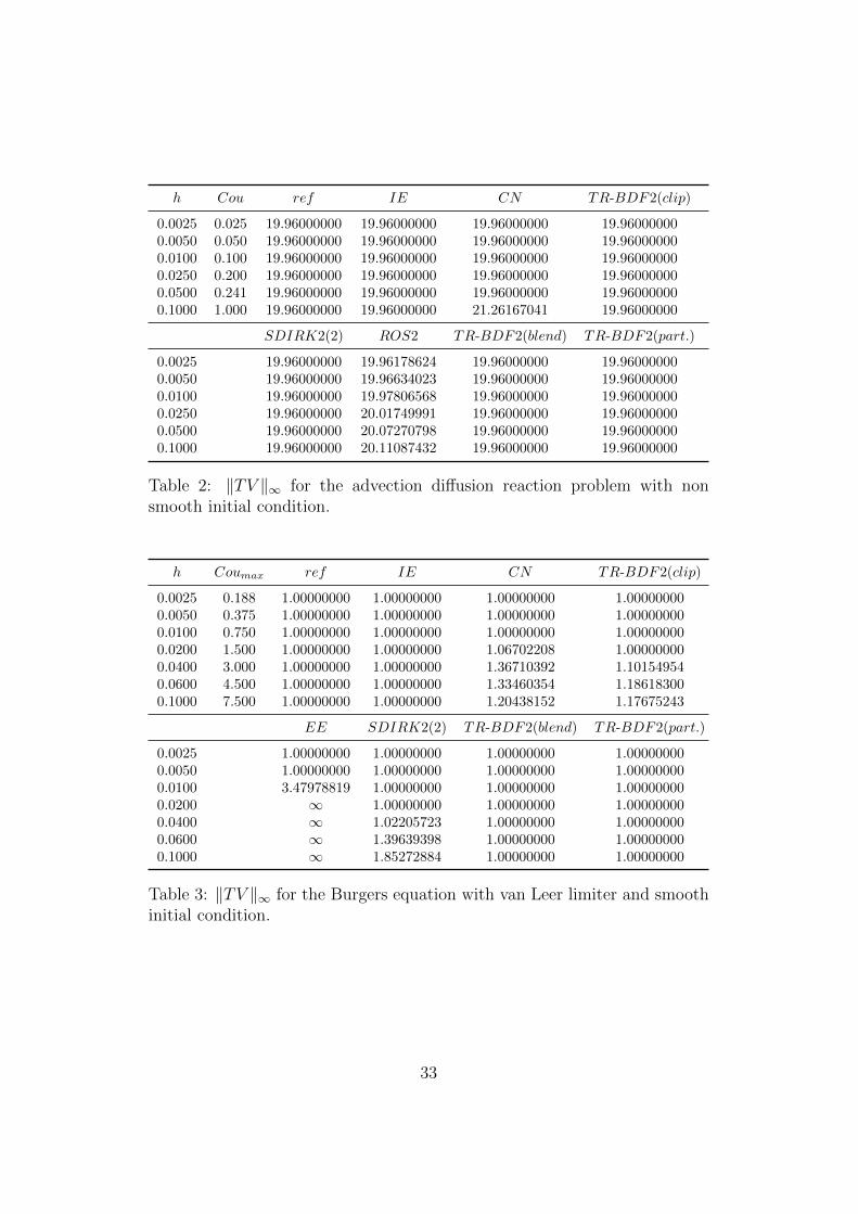
Here below we report the tables of the TV seminorm measured innumerical experiments to show that TV violations closely follow theexpected behaviour from the absolute monotonicity radius.
h Cou ref IE CN TR-BDF2(clip)
0.0025 0.25 2.00000000 2.00000000 2.00000000 2.000000000.0050 0.50 2.00000000 2.00000000 2.00000000 2.000000000.0100 1.00 2.00000000 2.00000000 2.00000000 2.000000000.0200 2.00 2.00000000 2.00000000 2.00000000 2.000000000.0241 2.41 2.00000000 2.00000000 2.37516991 2.000000000.0400 4.00 2.00000000 2.00000000 3.33333333 2.278580170.0600 6.00 2.00000000 2.00000000 4.06243821 2.390707720.1000 10.00 2.00000000 2.00000000 5.21857423 2.47739160
SDIRK2(2) ROS2 TR-BDF2(blend) TR-BDF2(part.)
0.0025 2.00000000 2.00877086 2.00000000 2.000000000.0050 2.00000000 2.02925347 2.00000000 2.000000000.0100 2.00000000 2.07630970 2.00000000 2.000000000.0200 2.00000000 2.14215613 2.00000000 2.000000000.0241 2.00000000 2.14775690 2.00000000 2.000000000.0400 2.00000000 2.12378933 2.00000000 2.000000000.0600 2.76800000 2.07354078 2.00000000 2.001143090.1000 3.73260435 2.01991743 2.00000000 2.00000000
Table 1: ‖TV ‖∞ for the advection problem with non smooth initial condition.
32
h Cou ref IE CN TR-BDF2(clip)
0.0025 0.025 19.96000000 19.96000000 19.96000000 19.960000000.0050 0.050 19.96000000 19.96000000 19.96000000 19.960000000.0100 0.100 19.96000000 19.96000000 19.96000000 19.960000000.0250 0.200 19.96000000 19.96000000 19.96000000 19.960000000.0500 0.241 19.96000000 19.96000000 19.96000000 19.960000000.1000 1.000 19.96000000 19.96000000 21.26167041 19.96000000
SDIRK2(2) ROS2 TR-BDF2(blend) TR-BDF2(part.)
0.0025 19.96000000 19.96178624 19.96000000 19.960000000.0050 19.96000000 19.96634023 19.96000000 19.960000000.0100 19.96000000 19.97806568 19.96000000 19.960000000.0250 19.96000000 20.01749991 19.96000000 19.960000000.0500 19.96000000 20.07270798 19.96000000 19.960000000.1000 19.96000000 20.11087432 19.96000000 19.96000000
Table 2: ‖TV ‖∞ for the advection diffusion reaction problem with nonsmooth initial condition.
h Coumax ref IE CN TR-BDF2(clip)
0.0025 0.188 1.00000000 1.00000000 1.00000000 1.000000000.0050 0.375 1.00000000 1.00000000 1.00000000 1.000000000.0100 0.750 1.00000000 1.00000000 1.00000000 1.000000000.0200 1.500 1.00000000 1.00000000 1.06702208 1.000000000.0400 3.000 1.00000000 1.00000000 1.36710392 1.101549540.0600 4.500 1.00000000 1.00000000 1.33460354 1.186183000.1000 7.500 1.00000000 1.00000000 1.20438152 1.17675243
EE SDIRK2(2) TR-BDF2(blend) TR-BDF2(part.)
0.0025 1.00000000 1.00000000 1.00000000 1.000000000.0050 1.00000000 1.00000000 1.00000000 1.000000000.0100 3.47978819 1.00000000 1.00000000 1.000000000.0200 ∞ 1.00000000 1.00000000 1.000000000.0400 ∞ 1.02205723 1.00000000 1.000000000.0600 ∞ 1.39639398 1.00000000 1.000000000.1000 ∞ 1.85272884 1.00000000 1.00000000
Table 3: ‖TV ‖∞ for the Burgers equation with van Leer limiter and smoothinitial condition.
33

h Coumax ref IE CN TR-BDF2(clip)
0.0010 0.2206 1.00000000 1.00000000 1.00000000 1.000000000.0025 0.5514 1.00000000 1.00000000 1.00000000 1.000000000.0050 1.1007 1.00000000 1.00000001 1.00000000 1.000000000.0075 1.6543 1.00000000 1.00000000 1.27084161 1.045195010.0100 2.2007 1.00000000 1.00000000 1.40310073 1.186713750.0150 3.3010 1.00000000 1.00000000 8.09702136 1.322718890.0250 5.5037 1.00000000 1.00000000 16.39900045 12.48391471
EE SDIRK2(2) TR-BDF2(blend) TR-BDF2(part.)
0.0010 1.00000000 1.00000000 1.00000000 1.000000000.0025 1.00000000 1.00000000 1.00000000 1.000000000.0050 1.87710600 1.00000000 1.00000000 1.000000000.0075 6.74722895 1.00000000 1.00000000 1.000000000.0100 21.35210300 1.00000000 1.00000001 1.004956310.0150 21.10782320 1.28222058 1.00000000 1.030924030.0250 19.65284356 1.57372343 1.00000000 1.00663983
Table 4: ‖TV ‖∞ for the Buckley-Leverett equation with Koren limiter andnon smooth initial condition.
Acknowledgements
A.D.R. would like to thank Tenova S.p.A. for sponsoring his ExecutivePhD at Politecnico di Milano and all the faculty members at the De-partment of Mathematics for their continuous support. L.B. acknowl-edges financial support from the INDAM - GNCS project ’Metodinumerici semi-impliciti e semi-Lagrangiani per sistemi iperbolici dileggi di bilancio’. Useful discussions with L. Formaggia and A. Scottion the topics studied in this paper are kindly acknowledged.
References
[1] R.E. Bank, W.M. Coughran, W. Fichtner, E.H. Grosse, D.J.Rose, and R.K. Smith. Transient simulation of silicon devicesand circuits. IEEE Transactions on Electron Devices, 32:1992–2007, 1985.
[2] A. Bellen, Z. Jackiewicz, and M. Zennaro. Contractivity of wave-form relaxation Runge-Kutta iterations and related limit meth-ods for dissipative systems in the maximum norm. SIAM Journalof Numerical Analysis, 31(2):499–523, 1994.
34

[3] A. Bellen and L. Torelli. Unconditional contractivity in the max-imum norm of diagonally split Runge-Kutta methods. SIAMJournal of Numerical Analysis, 34(2):528–543, 1997.
[4] E. Bertolazzi. Positive and conservative schemes for mass actionkinetics. Computers & Mathematics with Applications, 32(6):29–43, 1996.
[5] H. Burchard, E. Deleersnijder, and A. Meister. A high-orderconservative Patankar-type discretisation for stiff systems ofproduction-destruction equations. Applied Numerical Mathemat-ics, 47:1–30, 2003.
[6] J. Butcher and D. Chen. A new type of singly-implicit Runge-Kutta method. Applied Numerical Mathematics, 34:179–188,2000.
[7] E.M. Constantinescu and A. Sandu. Multirate timesteppingmethods for hyperbolic conservation laws. Journal of ScientificComputing, 33:239–278, 2007.
[8] K. Dekker and J.G. Verwer. Stability of Runge-Kutta Methods forStiff Nonlinear Differential Equations. Elsevier-North Holland,Amsterdam, 1984.
[9] L. Ferracina and M.N. Spijker. Stepsize restrictions for the Total-Variation-Diminishing property in general Runge-Kutta meth-ods. SIAM Journal of Numerical Analysis, 42(3):1073–1093,2004.
[10] L. Ferracina and M.N. Spijker. An extension and analysis of theShu-Osher representation of Runge-Kutta methods. Mathematicsof Computation, 74(249):201–219, 2005.
[11] L. Ferracina and M.N. Spijker. Strong stability of singly-diagonally-implicit Runge-Kutta methods. Applied NumericalMathematics, 58:1675–1686, 2008.
[12] L. Formaggia and A. Scotti. Positivity and conservation proper-ties of some integration schemes for mass action kinetics. SIAMJournal of Numerical Analysis, 49(3):1267–1288, 2011.
[13] F.X. Giraldo, J.F. Kelly, and E.M. Constantinescu. Implicit-explicit formulations of a three-dimensional nonhydrostatic uni-fied model of the atmosphere (NUMA). SIAM Journal of Scien-tific Computing, 35(5):1162–1194, 2013.
[14] S. Gottlieb, D. Ketcheson, and C.-W. Shu. Strong Stability Pre-serving Runge-Kutta and Multistep Time Discretizations. WorldScientific, Singapore, 2011.
35

[15] S. Gottlieb, C.W. Shu, and E. Tadmor. Strong stability-preserving high-order time discretization methods. SIAM Review,43(1):89–112, 2001.
[16] E. Hairer, S.P. Nørsett, and G. Wanner. Solving Ordinary Dif-ferential Equations I: Nonstiff Problems. Springer-Verlag, BerlinHeidelberg, 3rd corr. edition, 2008.
[17] E. Hairer and G. Wanner. Solving Ordinary Differential Equa-tions II: Stiff and Differential-Algebraic Problems. Springer-Verlag, Berlin Heidelberg, 2nd rev. edition, 2002.
[18] I. Higueras. On strong stability preserving time discretizationmethods. Journal of Scientific Computing, 21:193–223, 2004.
[19] I. Higueras. Monotonicity for Runge-Kutta methods: inner prod-uct norms. Journal of Scientific Computing, 24(1):97–117, 2005.
[20] I. Higueras. Representations of Runge-Kutta methods and strongstability preserving methods. SIAM Journal of Numerical Anal-ysis, 43(3):924–948, 2005.
[21] I. Higueras. Strong stability for Runge-Kutta schemes on aclass of nonlinear problems. Journal of Scientific Computing,57(3):518–535, 2005.
[22] I. Higueras. Strong stability for additive Runge-Kutta methods.SIAM Journal of Numerical Analysis, 44(4):1735–1758, 2006.
[23] I. Higueras and T. Roldan. Stage value predictors for additiveand partitioned Runge-Kutta methods. Applied Numerical Math-ematics, 56:1–18, 2006.
[24] M.E. Hosea and L.F. Shampine. Analysis and implementation ofTR-BDF2. Applied Numerical Mathematics, 20:21–37, 1996.
[25] W. Hundsdorfer, A. Mozartova, and M.N. Spijker. Special bound-edness properties in numerical initial value problems. BIT,51(4):909–936, 2011.
[26] W. Hundsdorfer, S.J. Ruuth, and R.J. Spiteri. Monotonicity-preserving linear multistep methods. SIAM Journal of NumericalAnalysis, 41(2):605–623, 2003.
[27] W. Hundsdorfer and M.N. Spijker. Boundedness and strong sta-bility of Runge-Kutta methods. Mathematics of Computation,80(274):863–886, 2011.
[28] W. Hundsdorfer and J. Verwer. Numerical Solution of Time-Dependent Advection-Diffusion-Reaction Equations. Springer-Verlag, Berlin Heidelberg, 2003.
36

[29] D.I. Ketcheson, S. Gottlieb, and C.B. Macdonald. Strong stabil-ity preserving two-step Runge-Kutta methods. SIAM Journal ofNumerical Analysis, 49(9):2618–2639, 2011.
[30] D.I. Ketcheson, C.B. Macdonald, and S. Gottlieb. Optimal im-plicit strong stability preserving Runge-Kutta methods. AppliedNumerical Mathematics, 59:373–392, 2009.
[31] J.F.B.M. Kraaijevanger. Contractivity of Runge-Kutta methods.BIT, 31:482–528, 1991.
[32] R. Lefever and G. Nicolis. Chemical instabilities and sustainedoscillations. Journal of Theoretical Biology, 30:267–284, 1971.
[33] R.J. LeVeque. Finite Volume Methods for Hyperbolic Problems.Cambridge University Press, 2002.
[34] C.B. Macdonald, S. Gottlieb, and S.J. Ruuth. A numerical studyof diagonally split Runge-Kutta methods for PDEs with discon-tinuities. Journal of Scientific Computing, 35:89–112, 2008.
[35] A. Sandu. Positive numerical integration methods for chemicalkinetic systems. Journal of Computational Physics, 170:589–602,2001.
[36] C.W. Shu. Total-Variation-Diminishing time discretiza-tion. SIAM Journal on Scientific and Statistical Computing,9(6):10731084, 1988.
[37] C.W. Shu and S. Osher. Efficient implementation of essentiallynon-oscillatory shock-capturing schemes. Journal of Computa-tional Physics, 77:439–471, 1988.
[38] M.N. Spijker. Contractivity in the numerical solution of initialvalue problems. Numerische Mathematik, 42(3):271–290, 1983.
[39] M.N. Spijker. Stepsize conditions for general monotonicity innumerical initial value problems. SIAM Journal of NumericalAnalysis, 45(3):1226–1245, 2007.
[40] B. Sportisse. An analysis of operator splitting techniques in thestiff case. Journal of Computational Physics, 161:140–168, 2000.
[41] G. Tumolo and L. Bonaventura. A semi-implicit, semi-Lagrangian, DG framework for adaptive numerical weather pre-diction. Quarterly Journal of the Royal Meteorological Society,DOI: 10.1002/qj.2544, 2015.
[42] J.A. van de Griend and J.F.B.M. Kraaijevanger. Absolute mono-tonicity of rational functions occurring in the numerical solutionof initial value problems. Numerische Mathematik, 49(4):413–424,1986.
37

[43] S. van Veldhuizen, C. Vuik, and C.R. Klein. A note on the nu-merical simulation of Kleijn’s benchmark problem. Report 06-15,Delft University of Technology, Dept. of Applied MathematicalAnalysis, 2006.
[44] S. van Veldhuizen, C. Vuik, and C.R. Klein. Comparison ofODE methods for laminar reacting gas flow simulations. Numer-ical Methods for Partial Differential Equations, 24(3):1037–1054,2008.
[45] J.G. Verwer, E.J. Spee, J.G. Blom, and W. Hundsdorfer. Asecond-order Rosenbrock method applied to photochemical dis-persion problems. SIAM Journal of Scientific Computing,20(4):1456–1480, 1999.
38