Monotonicity formulas and applications infree boundary problems

ANDERS EDQUIST

Doctoral ThesisStockholm, Sweden 2010

TRITA-MAT-10-MA-04ISSN 1401-2778ISRN KTH/MAT/DA 10/03-SEISBN 978-91-7415-595-2

KTHInstitutionen för Matematik

100 44 StockholmSWEDEN

Akademisk avhandling som med tillstånd av Kungl Tekniska högskolan fram-lägges till offentlig granskning för avläggande av teknologie doktorsexameni matematik fredagen den 7 maj 2010 kl 13.00 i sal F3, Kungl Tekniskahögskolan, Lindstedtsvägen 26, Stockholm.

c© Anders Edquist, 2010

Tryck: Universitetsservice US AB

iii

Abstract

This thesis consists of three papers devoted to the study of monotonicity for-mulas and their applications in elliptic and parabolic free boundary problems.

The first paper concerns an inhomogeneous parabolic problem. We obtainglobal and local almost monotonicity formulas and apply one of them to showa regularity result of a problem that arises in connection with continuation of heatpotentials.

In the second paper, we consider an elliptic two-phase problem with coeffi-cients bellow the Lipschitz threshold. Optimal C1,1 regularity of the solution anda regularity result of the free boundary are established.

The third and last paper deals with a parabolic free boundary problem withHölder continuous coefficients. Optimal C1,1 ∩ C0,1 regularity of the solution isproven.

iv

Sammanfattning

Denna avhandling består av tre vetenskapliga artiklar som alla behandlar mo-notonitetsformler och deras tillämpningar inom frirandsproblem.

I den första artikeln studeras ett inhomogent paraboliskt problem. Vi visar lo-kala och globala monotonicitetssatser. Den lokala versionen tillämpar vi för att visaett regularitetsresultat för ett problem som uppstår vid utvidgning av värmepoten-tialer.

I den andra artikeln betraktar vi ett elliptiskt frirandsproblem med två faser,där koefficienterna inte uppnår lipschitzregularitet. Vi visar optimal C1,1 regularitetav lösningen och ett regularitetsresultat för friranden.

Den tredje och sista artikeln berör ett paraboliskt frirandsproblem med hölder-kontinuerliga koefficienter. Optimal C1,1 ∩ C0,1 regularitet av lösningen visas.

Acknowledgements

I thank ESF Global, STINT and the Royal Swedish Academy of Sciences fortravel support.

During my time at KTH many people have supported me, some of you Imention here. First and foremost, I would like to thank Henrik Shahgholianfor being a great supervisor. He has always supplied me with interesting,challenging problems and with enthusiasm spend his time helping me.

I also want to thank Arshak Petrosyan. During my stay at Purdue Uni-versity, Arshak was a great tutor and a very generous host.

For a couple of years I shared office with Erik Lindgren. I thank Erik forgood coorporation and for all the fun we had during this time. I also wantto mention Farid Bozorgnia, Avetik Arakelyan and all other friends at thedepartment for your help and for the great time we spent together.

Last but not the least, I am grateful to Anna for your never endingsupport and encoragement. Together with Daniel we have shared manygreat moments.

v

Contents

Acknowledgements v

Contents vi

Introduction and summary

1 Free boundary problems 11.1 The obstacle problem . . . . . . . . . . . . . . . . . . . . . . . 11.2 Two-phase free boundary problems . . . . . . . . . . . . . . . 41.3 Option pricing . . . . . . . . . . . . . . . . . . . . . . . . . . 51.4 Mathematical formulation . . . . . . . . . . . . . . . . . . . . 81.5 Monotonicity techniques . . . . . . . . . . . . . . . . . . . . . 101.6 Regularity properties . . . . . . . . . . . . . . . . . . . . . . . 11

2 Summary of Paper I 152.1 The global formula . . . . . . . . . . . . . . . . . . . . . . . . 152.2 The local formula . . . . . . . . . . . . . . . . . . . . . . . . . 172.3 An application . . . . . . . . . . . . . . . . . . . . . . . . . . 18

3 Summary of Paper II 193.1 Background . . . . . . . . . . . . . . . . . . . . . . . . . . . . 193.2 Regularity of the solution . . . . . . . . . . . . . . . . . . . . 193.3 Free boundary regularity . . . . . . . . . . . . . . . . . . . . . 20

4 Summary of Paper III 234.1 Background . . . . . . . . . . . . . . . . . . . . . . . . . . . . 234.2 Regularity of the solution . . . . . . . . . . . . . . . . . . . . 24

vi

vii

References 27

Scientific papers

Paper IA parabolic almost monotonicity formula(joint with Arshak Petrosyan)Math. Ann. 341 (2008), p. 429–454

Paper IIOn the two-phase membrane problem with coefficients below the Lip-

schitz threshold(joint with Erik Lindgren and Henrik Shahgholian)Annales de l’Institut Henri Poincaré - Analyse non linéaire 26,

(2009), p. 2359–2372

Paper IIIRegularity of a parabolic free boundary problem with Hölder contin-

uous coefficients(joint with Erik Lindgren)Preprint

Chapter 1

Introduction to free boundaryproblems

In this chapter we introduce free boundary problems (FBPs). The first threesections are devoted to examples of where free boundary problems arise.This is followed by a classification of relevant FBPs and a discussion of someimportant results in elliptic and parabolic FBPs. In the end of this chapter,we give some ideas of how regularity results can be obtained for FBPs.

1.1 The obstacle problem

Consider a circular trampoline which consists of an elastic membrane fixedto its boundary. Since the tension force is large compared to gravity, itis reasonable to neglect gravity. Therefore, the membrane will be flat. Ifinstead the membrane of the trampoline is obstructed by an obstacle, whatwill be the new form of the membrane?

In order to answer this question we need to know the principles determin-ing the shape of the membrane. From physics it is well known that an elasticmembrane will take the shape that minimizes the tension energy, which willbe proportional to the area of the membrane. We introduce h(x) as thevertical position and D as the domain of the membrane. The area of themembrane can be calculated as:

A =∫

D

√1 + |∇h(x)|2 dx.

1

2 CHAPTER 1.

Figure 1.1: The membrane is pushed up by an obstacle.

For small disturbances from the equilibrium we can approximate the areawith

A ≈ |D|+ 12

∫D|∇h|2 dx.

Since the membrane is fixed at its boundary we have the boundary con-dition h = g on ∂D, where g(x) represents the vertical position of the fixedboundary. Furthermore the trampoline has to be above the obstacle, i.e.h ≥ ψ. An example of this setting is shown in Figure 1.1.

The approximated problem is to minimize

J(h) =∫

D|∇h|2 dx,

while h = g on ∂D and h ≥ ψ in D. This is called the variational form ofthe obstacle problem and J is usually referred to as the Dirichlet energy.

PDE formulationSuppose v is a minimizer to the variational form of the above problem andlet

f(t) = J(v + tφ) =∫

D|∇(v + tφ)|2dx,

where φ ∈ C∞0 (D) and t is a real number. First consider both φ and t as

non-negative. Since v is a minimizer f ′(0) = 2∫D∇v∇φ dx is non-negative.

1.1. THE OBSTACLE PROBLEM 3

Γ

u > 0

u = 0

Figure 1.2: The different phases of the domain in Figure 1.1. The dashedline represents the free boundary Γ.

By integrating this relation by parts, we obtain that v is superharmonic inthe distributional sense, which is ∆v ≤ 0.

The next step is to relax the sign restrictions on t and φ and considerφ ∈ C∞

0 (D ∩ v > ψ). For small enough t we have v + tφ > ψ, and sincev is a minimizer, f ′(0) = 0. From this we obtain that v is harmonic outsidethe coincidence set.

In order to simplify the expressions we introduce a new function u = v−ψ.For u we have the following relation

∆u = (−∆ψ)χu>0 in D,

where u = g−ψ on ∂D. This is called the partial differential equation (PDE)version of the obstacle problem.

Using integration by parts it follows that, for an appropriate class offunctions, the variational formulation can be obtained from the PDE formu-lation. This means that the two formulations are equivalent.

Free boundaryIn the above example, the membrane touches the obstacle in a part of themembrane. The set where contact occurs, u = 0, is called the coincidenceset while the set where the membrane does not touch the boundary u > 0is called the non-coincidence set. The delimiter between those sets, Γ(u) =∂u > 0 ∩D, is usually referred to as the free boundary.

4 CHAPTER 1.

1.2 Examples of two-phase free boundaryproblems

In the PDE formulation of the of the obstacle problem the solution, u, isnonnegative. If we consider FBPs without sign restrictions we can modelseveral other problems. In this section we give two such examples.

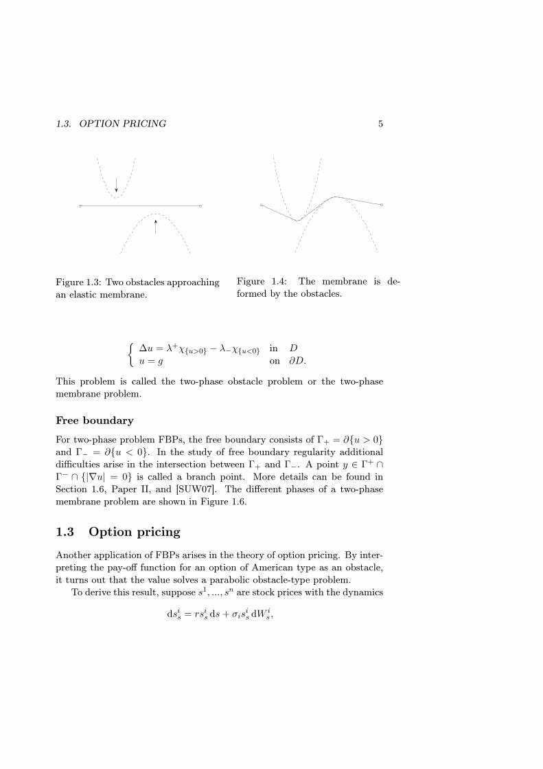
The double obstacle problemAs in the one-phase obstacle problem, consider an elastic membrane fixedat its boundary. Here we have two obstacles, ψ1 from below, and ψ2 fromabove, see Figure 1.3 and Figure 1.4. Again the problem is to determine theshape of the membrane.

The form will be determined by minimization of the Dirichlet energy

J(v) =∫

D|∇v|2 dx, (1.2.1)

over the set K = v−g ∈W 1,20 (D) |ψ1 ≤ f ≤ ψ2. If we use u = v−ψ1+ψ2,

the corresponding Euler-Lagrange equation will be

∆u = λ+χu>0 − λ−χu<0 in D, (1.2.2)

where λ+ = −∆ψ1 and λ− = −∆ψ2. This is called the double obstacleproblem.

Membrane applicationAnother application of two-phase FBPs may arise in a tank filled with twoliquids with different densities. If a membrane, which has density in betweenthe densities of the liquids, is fixed in the tank, in such a way that some partof the membrane is below the heavy liquid while the rest is above the lighterliquid, then the membrane due to gravity will be pushed up in the heavierphase and pushed down in the lighter, see Figure 1.5. The equilibrium statewill be given by a minimization of the functional∫

D

|∇u|2

2+ λ+u

+ − λ−u− dx,

with boundary values u = g, where g(x) represent the position at the fixedboundary, which is equivalent with

1.3. OPTION PRICING 5

Figure 1.3: Two obstacles approachingan elastic membrane.

Figure 1.4: The membrane is de-formed by the obstacles.

∆u = λ+χu>0 − λ−χu<0 in D

u = g on ∂D.

This problem is called the two-phase obstacle problem or the two-phasemembrane problem.

Free boundaryFor two-phase problem FBPs, the free boundary consists of Γ+ = ∂u > 0and Γ− = ∂u < 0. In the study of free boundary regularity additionaldifficulties arise in the intersection between Γ+ and Γ−. A point y ∈ Γ+ ∩Γ− ∩ |∇u| = 0 is called a branch point. More details can be found inSection 1.6, Paper II, and [SUW07]. The different phases of a two-phasemembrane problem are shown in Figure 1.6.

1.3 Option pricingAnother application of FBPs arises in the theory of option pricing. By inter-preting the pay-off function for an option of American type as an obstacle,it turns out that the value solves a parabolic obstacle-type problem.

To derive this result, suppose s1, ..., sn are stock prices with the dynamics

dsis = rsi

s ds+ σisis dW

is ,

6 CHAPTER 1.

Figure 1.5: A membrane fixed in atank filled with two liquids. The heav-ier liquid pushes the membrane up,while the lighter pushes it down. Thefree boundary is a single point at theboundary layer between the liquids.

Γ

u < 0

x1 x2

u > 0

x3

Γ+

u = 0

Γ−

Figure 1.6: Example of the differentphases in a two-phase problem in a twodimensional domain. x1 is a two-phasepoint, x2 is a branch point and x3 is aone-phase point.

where r is the continuous interest rate, σi the volatility and dW is the Brow-

nian motions. The correlations between the Brownian motions are denotedρij .

First we consider a stock option based on n stocks S = (s1, ..., sn) whichgives the holder of the option the right to exercise the option with pay-offψ(S) at exercise time T . This is called a stock option of European type. Tocalculate expected values the probability measure Q is chosen according tothe arbitrage free market assumption, for details see Øksendal [Øks03]. Thisis the probability measure that makes Ss/e

r(s−t) into a martingale. UnderQ the value of the option at a state (S, t) is given by

ve(S, t) = EQ(e−r(T−t)ψ(ST )|St = S).

If instead we have an option which can be exerised at any time we saythat the option is of American type. The value of this option is given by

va(S, t) = supt≤t′≤T

ve(S, t′).

Clearly, for any pay-off function ψ, the American option is worth at leastas much as the European. Due to the Feyman-Kac formula [Øks03] we know

1.3. OPTION PRICING 7

00.5

11.5

2

0

0.5

1

0

0.1

0.2

0.3

0.4

0.5

0.6

0.7

0.8

0.9

1

St

v

Figure 1.7: The value of an American put option according to the Black-Scholes model, a parabolic obstacle problem.

that the value of the European option solves the Black-Scholes PDE∂tve + Lve = 0 in Rn × [0, T ),ve(S, T ) = ψ(S) in Rn,

where

Lf =12

n∑i,j=1

ρijσiσjsisj∂si∂sjf +n∑

i=1

rsi∂sif − rf.

Since xiρijxj = (xi/σi)Cij(xj/σj), where Cij is the covariance matrix, it fol-lows from the positive semidefiniteness of Cij that ρij is a positive semidefi-nite matrix [Mil75]. If we exclude the perfectly correlated and anticorrelatedcases then the correlation matrix is positive definite. Therefore, L is an

8 CHAPTER 1.

elliptic operator. For the American option the problem becomes∂tva + Lva ≥ 0(va − ψ)(∂tva + Lva) = 0va(S, T ) = ψ(S).

If we impose a nonnegative function u = va − ψ we can rewrite the problemas

(∂t + L)u = −(∂t + L)ψχu>0∂tu+ Lu ≥ ∂tψ + Lψu(S, T ) = 0.

This is a parabolic free boundary problem with ∂u > 0 as the free bound-ary.

To solve the problem numerically we need to have a bounded domain.This can sometimes be done by studying the asymptotic behavior of theoption. For example, consider an American put option based on one stockonly. The pay-off of this option is ψ(S) = (K−S)+ at any time up to expiry.Far away from the strike price (S = K) we can approximate the value withψ(S) and therefore we use this as boundary value. An example solution isplotted in Figure 1.7.

Exercise region

For a holder of an American option it is crucial to know when it is favorableto exercise it. The set v = ψ is called the early exercise region of an option;this is the same as the coincidence set u = 0 of the equation. An optimalstrategy is to exercise the option whenever the free boundary is reached.Therefore, the free boundary of this parabolic obstacle type problem givesus the optimal strategy.

1.4 Mathematical formulation

In the previous sections some practical examples of FBPs were explained.A common feature is the presence of an a priori unknown front called thefree boundary. The free boundary divides the domain into regions where thePDE is inhomogeneous and homogeneous respectively.

1.4. MATHEMATICAL FORMULATION 9

In this thesis we consider parabolic and elliptic problems. The ellipticproblems which we study all fit into the following free boundary problemformulation:

F (D2u) = g(x)χΩ(u) in Du = φ on ∂D. (1.4.1)

The parabolic problems can be formulated as:ut + F (D2u) = g(x, t)χΩ(u) in D × (t0, t1]u = φ on ∂D × (t0, t1)u = γ on D × t0.

(1.4.2)

In both cases F is a bounded elliptic function on matrices and D is a smoothregion in Rn. The coefficient function g, the boundary values φ and the initialvales γ are assumed to be continuous.

In this thesis, one- and two-phase problems are of special interest. IfΩ(u) = u > 0 we denote the problem as one-phase. When it is possibleto split Ω(u) into two parts as Ω+(u) = u > 0 and Ω−(u) = u < 0, werefer to the problem as of two-phase type.

Elliptic and parabolic problems

In free boundary problems, parabolic and elliptic problems are closely re-lated. The reason for this is the similarities in the general theory of parabolicand elliptic PDE. Two results which are of special interest, are the maximumprinciple and Harnack’s lemma.

To formulate these two results, let L be an elliptic or parabolic operator.The maximum principle states that if Lu ≤ 0, then u attains its maximumat the boundary. For a non-negative function u with Lu = 0, Harnack’sinequality tells us that the infimum and supremum are comparable, in anycompact set, in the sense

supx∈K

u ≤ CK infx∈K

u.

Existence and uniqueness

The uniqueness and existence of solutions to many free boundary problemsfollow from general methods in the calculus of variations. In a region D ⊂

10 CHAPTER 1.

Rn, let

J(v) =∫

DL(∇v(x), v(x), x) dx

where v is a real valued function. If L is convex in the first argument, coerciveand lower semi-continuous, then for any non-empty convex set K there existsa unique v0 ∈ K such that

J(v0) = minv∈K

J(v).

Proofs and more details regarding this result can be found in [Str90] and[Eva98].

As an example, we consider the obstacle problem. Our minimizationproblem is

minv∈K

J(v) =∫

D|∇v|2 dx

where K = v − g ∈ W 1,20 (D) | v ≥ ψ. If ψ is sub-harmonic, then K is

convex and all the above requirements are fulfilled.The existence and uniqueness for the PDE version follow from the equiv-

alence with the variational formulation. However, if we cannot prove equiv-alence the above result does not help us. This is indeed sometimes the case.For example, in the two phase p-obstacle problem with p < 2 there are noknown proofs of equivalence, see [EL09].

1.5 Monotonicity techniques in free boundaryproblems

There are two different types of monotonicity formulas which both are im-portant tools in the study of regularity in free boundary problems. In thissection the original version of each type is presented.

The regularity of the solutions [Fre72] and the free boundary [Caf77]of the obstacle problem were first obtained with variational methods. In1984 Alt, Caffarelli and Friedman [ACF84] presented a monotonicity for-mula for sub-harmonic functions, which was a breakthrough in the study offree boundary regularity. Since then, PDE methods have represented thedominating approach to prove regularity in FBPs.

The monotonicity formula can be formulated as follows:

1.6. REGULARITY PROPERTIES 11

Theorem 1.1. (ACF monotonicity formula) Let u be a continuous functionin BR with |∇u| ∈ L2(BR). If u is harmonic in BR \ u = 0 and vanishesat the origin, then

Φ(r) =1r2

∫Br

|∇u+|2

|x|n−2dx · 1

r2

∫Br

|∇u−|2

|x|n−2dx

is bounded and increasing in 0 < r < R.

This formula was generalized into an almost monotonicity formula [CJK02]which has been used for proving optimal regularity of the solution in manyFBPs, for example in [Sha03], [Caf98] and [Ura01]. In Paper I a parabolicalmost monotonicity formula of similar type is proved.

In 1999 Weiss presented another type of monotonicity formula [Wei99].

Theorem 1.2. Assume we have a FBP as in (1.4.1) and suppose F is thetrace operator, g = 1, Ω(u) = u > 0 and Bδ ⊂ Ω. The Weiss energy

W (r;u) =∫

Br

|∇u|2 + u+ dx− 2r−n−3

∫∂Br

u2 dσ,

is monotonously increasing for 0 < r < δ.

This formula has been used to classify global solutions, which in turn isused to obtain regularity results for the free boundary. A parabolic versionof this formula is established in Paper III.

1.6 Regularity propertiesAfter the existence and uniqueness of a PDE has been established an obviousissue to study is the qualitative behavior of the solution in terms of regularity.This is also important when solving problems numerically. There are nogeneral methods for establishing regularity in FBPs. Instead some importanttechniques and common arguments to tackle such problems are presented inthis section.

Interior regularity

By interior regularity we mean regularity of the solution. The optimal regu-larity is usually proved using a minimum regularity criterion combined with

12 CHAPTER 1.

an explicit solution, showing that the regularity obtained is the best possible.As an example, consider the following obstacle problem in one dimension:

∆u = χu>0

in D = (−1, 1), with boundary values u(−1) = 0 and u(1) = 1. Thisproblem has the solution u = |x+|2/2. Therefore the optimal regularity forthe obstacle problem in general cannot be better than C1,1(D).

Excluding points at the free boundary and its neighborhood we haveregularity estimates of the solution from classic elliptic or parabolic theory.Therefore we turn our attention to points close to the free boundary. Findinga regularity estimate for the solution often involves scaling of the problem.Let us consider the elliptic case. If we have a solution u in B1, then thefunction

ur(x) =u(rx)rγ

often is a solution to the same problem in B1/r. Now we expect the optimalregularity to be Cbγc,(γ−bγc). This is however not true in general. Oneexample where the solution is not the Cbγc,(γ−bγc) is the unstable obstacleproblem, ∆u = −χu>0, see [AW06] or [MW07].

For proving optimal regularity we start by establishing Hölder-α regu-larity for any 0 < α < 1. If we restrict our discussion to the one- andtwo-phase, obstacle problems, ∆u is bounded. Therefore, for any compactsubset, Hölder regularity follows from the Calderon-Zygmund inequality, fordetails see [GT83].

Again, close to the free boundary we have classical estimates, thereforethe main issue is to prove a growth estimate close to the free boundary. Fora point x0 on the free boundary we are expecting

supBr(x0)

|u| ≤ Crγ

for small enough r. This is proved for a wide class of elliptic FBPs in[KS00]. The proof is based on scaling arguments combined with generalelliptic theory, including the maximum principle.

NondegeneracyIn the study of optimal regularity of the solution, an upper bound of thegrowth-rate is established. Nondegeneracy is the opposite, i.e. the control of

1.6. REGULARITY PROPERTIES 13

a. b. c.

Figure 1.8: Blow-ups in one dimension. The columns represent blow-ups of(a) a differentiable point, (b) a corner point and (c) a cusp point.

the minimum growth rate close to the free boundary. This will be importantwhen we use zoom-in techniques to obtain free boundary regularity. For aproblem that has a scaling of order γ we will expect

supBr(x0)

|u| ≥ Crγ ,

for x0 a point on the free boundary. For many FBPs this estimate followsfrom the maximum principle.

When we study the regularity of the free boundary the first step is toprove that the Hn−1-measure of the free boundary is finite (for more onthe Hausdorff measure, see [EG92]). The proof of this for various one- andtwo-phase obstacle problems is based on nondegeneracy.

The aim of the regularity theory of the free boundary is often to provethat the free boundary is a graph of a C1 function. The idea is to zoom-inand observe the behavior of the solution. For a blow-up at x0 define

ur(x) =u(rx+ x0)

rα.

Then we say that for a sequence rj 0, u0(x) = limj→∞ urj is a blow-up. In order to reach any conclusion from this we need to know that ur

remains bounded without identically vanishing. The boundedness follows

14 CHAPTER 1.

from optimal regularity while the nondegeneracy guarantees that the solutiondoes not identically vanish.

The limiting function of the rescalings, u0, will be a function on Rn.Therefore u0 is called a global solution. The existence of a limit functionand the classification of it will often follow from Theorem 1.2. Figure 1.8,shows examples of what may occur in one dimension.

Chapter 2

Summary of Paper I

In this paper we establish an almost monotonicity formula for a pair of non-negative functions u± satisfying

(∆− ∂s)u± ≥ −1,u+ · u− = 0

in S1 = Rn × (−1, 0]. We also prove a localized version of the formula andanother variant under stronger assumptions. At the end of the paper weuse the formula to prove a regularity estimate for a free boundary problemrelated to the caloric continuation of heat potentials.

As described in Section 1.5, monotonicity formulas are important toolsin FBPs. The almost monotonicity formula proven in this paper is a general-ization of the parabolic monotonicity formula in [Caf93] and it is a parabolicanalogue to the almost monotonicity formula in [CJK02]. Many of the ideasin this paper originates from [CJK02].

2.1 The global formula

A difference between elliptic and parabolic monotonicity formulas is that inthe elliptic case, monotonicity formulas are local in the sense that u± onlyhave to be defined in a finite ball. For the parabolic case u± need to bedefined in an infinite strip such as Sr = Rn × (−r2, 0]. Therefore we firsthave to establish a global formula.

15

16 CHAPTER 2.

Theorem 2.1. LetG(x, t) =

1(4πt)n/2

e−|x|2/4t

denote the heat kernel and let u+ and u− be two non-negative functions withmoderate growth and disjoint support that satisfy

(∆− ∂s)u± ≥ −1 in S1. (2.1.1)

Then for

A±(r) =∫∫

Sr

|∇u±|2G(x,−t) dx dt

the function

Φ(r) =A+(r)r2

A−(r)r2

satisfies

Φ(r) ≤ C(1 +A+(1) +A−(1))2, for 0 < r ≤ 1. (2.1.2)

This is a bound on Φ rather than a monotonicity result. The namemonotonicity formula is explained by the relation with the ACF monotonicityformula (see Theorem 1.1) and the use of the so called monotonicity functionΦ. The proof of the theorem follows the same structure as the proof of theelliptic almost monotonicity formula in [CJK02]. It consists of a technicalpart and an arithmetical part using a scaling argument.

In the technical part, gradient estimates and an estimate of Φ′ in termsof A± and Φ are established. This leads to recursive inequalities for A±k =A±(4−k) and b±k = 44kA±k . Since the inequalities are modified in an analoguesway to [CJK02], the purely arithmetic scaling argument, can be completelyrecycled.

The idea is to interpret b±k as the correctly rescaled version of A±. Thisis because

ur(x, t) =u(rx, r2t)

r2

satisfies(∂t −∆)ur ≤ −1

if and only if u satisfy the same relation and that∫∫S1

|∇ur|2G(x,−t) dx dt = r−4

∫∫Sr

|∇u|2G(x,−t) dx dt.

2.2. THE LOCAL FORMULA 17

The reason for studying A±k and b±k simultaneously is that A±k decreaseswith k while b±k is the correctly rescaled version of A± and therefore bk isconstant. Using the recursive relations this leads to the proof of the formula.The calculations are carried out in [CJK02].

2.2 The local formula

In order to apply the formula to functions defined in bounded domains weneed a local version. One way to localize the formula in (2.1.2) is to multiplythe solutions with a cut-off function, thus extending them to an infinite strip.This leads to errors in the computations in the proof. By controlling themwe can prove the localized formula.

Theorem 2.2. Suppose we have two non-negative, continuous L2(Q−3 ) func-

tions u±(x, s) with disjoint support that satisfy

(∆− ∂s)u± ≥ −1 in Q−3 ,

whereQ−

r = Br × (−r2, 0].

Let ψ ∈ C∞0 (Rn) be a cut-off function such that

0 ≤ ψ ≤ 1, suppψ ⊂ B2, ψ = 1 in B1.

Then if w±(x, s) = u±(x, s)ψ(x) for (x, s) ∈ S3, the function

Φ(r) = r−4A+(r)A−(r),

where

A±(r) =∫∫

Sr

|∇w±|2G(x,−t) dx dt,

satisfies

Φ(r) ≤ C(1 + ‖u+‖L2(Q−

3 ) + ‖u−‖L2(Q−3 )

)2for 0 < r ≤ 1.

18 CHAPTER 2.

2.3 A regularity applicationConsider the following parabolic FBP:

∆u− ∂su = f(x, s)χΩ in Q−1

Ω = Q−1 \ u = |∇u| = 0

sup |f(x, s)| ≤ K <∞.(2.3.1)

This problem arises in the theory of caloric continuation of heat potentials.If we impose as an additional condition that f is Lipschitz with respect tothe parabolic distance, which is

|f(x, t)− f(y, s)| ≤ L√|x− y|2 + |t− s| (2.3.2)

we can use the localized version of the almost monotonicity to prove thefollowing regularity theorem:

Theorem 2.3. Let u ∈ L∞(Q−1/4) be a solution to (2.3.1). Then there exists

a constant C such that

supQ−

1/4∩Ω

|∂xixju| ≤ C, supQ−

1/4∩Ω

|∂su| ≤ C, i, j = 1, ..., n.

The proof of the theorem is based on the quadratic growth of u, whichin turn can be proven by using Theorem 2.2.

Chapter 3

Summary of Paper II

This paper concerns the two-phase obstacle problem with coefficients belowthe Lipschitz threshold. We prove C1,1 regularity of the solution and thatthe free boundary is a union of two C1-graphs close to branching points.

3.1 Background

For two positive Hölder continuous functions λ+, λ−, and boundary datag ∈ H1(B1) ∩ L∞(B1), we study

∆u = λ+χu>0 − λ−χu<0 (3.1.1)

where u ∈ H1(B1). Existence and uniqueness follow from general varia-tional methods as described in Section 1.4. For details see [Wei01]. Theoptimal regularity of the two-phase problem has been studied in [Ura01] forλ± constants and in [Sha03] for λ± Lipschitz continuous functions. In bothcases optimal C1,1 regularity of the solution was obtained. In [SUW07], theregularity of the free boundary for Lipschitz coefficients was proven to bethe union of two C1-graphs. Here we generalize the regularity results to λ±Hölder continuous functions.

3.2 C1,1 regularity of the solution

As described in Section 1.6 the regularity of the solution away from the freeboundary is determined by interior estimates. Here the regularity of the

19

20 CHAPTER 3.

coefficients will determine the regularity in u > 0 and u < 0. Thereforethe remaining problem is to prove regularity close to ∂u 6= 0. The resultis stated as follows:

Theorem 3.1. Let u be a bounded solution to (3.1.1) in B1 with λ± Höldercontinuous positive functions bounded both from below and above. Then thereare constants r and C such that

‖u‖C1,1(Br) ≤ C.

To prove this result we use the following scaling:

vj(x) =uj(rjx+ y)

r2j.

First we consider a branch point y ∈ Γ+(u) ∩ Γ−(u) ∩ ∇u = 0. Up toa subsequence rj → 0 the rescaling converges to a global solution of thetwo-phase obstacle problem with constant coefficients and a branch-point atthe origin. This case is already classified in [Ura01].

If we instead have a point on the free boundary with a non-vanishinggradient, a similar method to the above, results in a limit function whichsolve

∆u = λ+χu>α·x − λ−χu<α·x in Rn.

If we assume quadratic growth of the solution and choose the coordinatessuch that α = −ae1, then the origin is a branch point. The only possiblesolutions to the above problem can be shown to be u1 = λ+

(x+1 )2

2 , u2 =

λ−(x−1 )2

2 or a sum of u1 and u2. The proof is based on the monotonicityformula in Theorem 1.1.

3.3 Free boundary regularity

Definition 3.2. (Reifenberg-flatness) A compact set in S ⊂ Rn is said to beδ-Reifenberg flat if, for any compact set K ⊂ Rn, there exists RK > 0 suchthat for every x ∈ K ∩S and every r ∈ (0, RK ] we have a hyperplane L(x, r)such that

dist(L(x, r) ∩Br(x), S ∩Br(x)) ≤ 2rδ.

3.3. FREE BOUNDARY REGULARITY 21

We define the modulus of flatness as

θK(r) = sup0<ρ≤r

(sup

x∈S∩K

dist(L(x, ρ) ∩Bρ(x), S ∩Bρ(x))ρ

).

A set is called Reifenberg vanishing if

limr→0

θK(r) = 0.

The principle idea in the proof of Reifenberg-flatness of the free boundaryis to trap u between the solution of the following problems:

∆u1 = λi+χu1>0 − λs

−χu1<0

∆u2 = λs+χu2>0 − λi

−χu2<0

where λi± = inf λ±(x) and λs

± = supλ±(x). The boundary values are thesame as for the original problem (3.1.1). Both the above problems haveconstant coefficients. For this case the free boundary is a graph of a C1-function [SUW07].

The distance between the free boundaries of u1 and u2 can be estimatedby

dist(Γ±(u1) ∩Br,Γ±(u2) ∩Br) ≤ C√

max(osc(λ±).

We apply this to the rescalings to obtain Reifenberg flatness of the freeboundary. This is stated in the following theorem:

Theorem 3.3. Suppose u is a solution with the same properties as in (3.1).Then if |∇u(y)| and dist(y,Γ±) both are bounded, there is a positive constantr such that both Γ+ ∩Br and Γ− ∩Br are Reifenberg vanishing sets.

Chapter 4

Summary of Paper III

In this paper we study a parabolic obstacle problem involving an operatorwith Hölder continuous coefficients. Under a combination of energetic andgeometric conditions we prove optimal C1,1

x ∩C0,1t regularity of the solution.

4.1 BackgroundWe consider the following problem

∆u− ∂tu = f(x)χu>0 in Q−1

u = |∇u| in Q−1 \ Ω

(4.1.1)

where f is assumed to be a Hölder continuous function and Q−r = Br ×

(−r2, 0]. In the same problem but with the restriction that f is constant thesolution has local C1,1

x ∩ C0,1t estimates [CPS04]. A corresponding elliptic

problem was studied in [PS07]. In that paper, the authors made the followingDini-type assumption on the modulus of continuity of f :∫ 1

0

ωf (r) log 1r

rdr <∞,

Under some energetic and geometric assumptions C1,1 regularity of the so-lution and C1 regularity of the free boundary were obtained. Our method isbased on the approach in [PS07].

In order to formulate the results we define the energy function and ageometrical measure of the coincidence set. We use the parabolic thickness

23

24 CHAPTER 4.

functionδ(u, r) = mindiam

Λ(u) ∩Q−r

r.

as a geometrical measure of the coincidence set. For v(x, t): Rn × R+ → Rthe Weiss energy is defined by

W (r; v, f) =1r4

∫ −r4

−4r2

∫Rn

(|∇v|2 + 2fv +

v2

t

)e−|x|

2/4tG(x,−t) dx dt,

whereG(x, t) =

1(4πt)n/2

e−|x|2/4t

is the heat kernel.For a local solution to 4.1.1 we prove that there exists a continuous

function F vanishing at the origin such that

W (r;u, f) + F (r)

is a monotonically nondecreasing function for 0 < r < 1/2. This is aparabolic version of Weiss monotonicity formula, Theorem 1.2.

4.2 Regularity of the solutionThe main result of this paper is the following regularity theorem:

Theorem 4.1. Assume that u is a local solution to (4.1.1) with appropriateproperties and An = 15f(0)/4. Then for ε > 0 there exists rε > 0 such thatif for some 0 < r0 < rε

δ(r0/2, u) ≥ ε and W (r0;u, f) < 2An − ε (4.2.1)

then

‖u‖C1,1

x ∩C0,1t (Qcε,r0

)≤ Cε,r0 for every 0 < r ≤ r0 (4.2.2)

for some small cε,r0 .

The first step of the proof is to show quadratic growth of the solution. Havingdone this, we use induction on the scaling

vk(x) =v(dk

εx, d2kε t)

d2kε

.

4.2. REGULARITY OF THE SOLUTION 25

The argument uses both the monotonicity properties ofW and the geometriccriterion.

The next step is to prove the regularity of the solution. Here we onlyneed to consider points close to the free boundary. We introduce

w =v(c+ x0, t+ t0)

f(x0, t0),

where (x0, t0) is a point on the free boundary. This results in the followingestimate on the solution:

v ≤ C dist((x, t),Γ)2.

Applying Schauder estimates at this result we can deduct the theorem.

References

[ACF84] Hans Wilhelm Alt, Luis A. Caffarelli, and Avner Friedman, Vari-ational problems with two phases and their free boundaries, Trans.Amer. Math. Soc. 282 (1984), no. 2, 431–461.

[AW06] J. Andersson and G. S. Weiss, Cross-shaped and degenerate singu-larities in an unstable elliptic free boundary problem, J. DifferentialEquations 228 (2006), no. 2, 633–640.

[Caf77] Luis A. Caffarelli, The regularity of free boundaries in higher di-mensions, Acta Math. 139 (1977), no. 3-4, 155–184.

[Caf93] , A monotonicity formula for heat functions in disjoint do-mains, Boundary value problems for partial differential equationsand applications, RMA Res. Notes Appl. Math., vol. 29, Masson,Paris, 1993, pp. 53–60.

[Caf98] L. A. Caffarelli, The obstacle problem revisited, J. Fourier Anal.Appl. 4 (1998), no. 4-5, 383–402.

[CJK02] Luis A. Caffarelli, David Jerison, and Carlos E. Kenig, Some newmonotonicity theorems with applications to free boundary problems,Ann. of Math. (2) 155 (2002), no. 2, 369–404.

[CPS04] Luis Caffarelli, Arshak Petrosyan, and Henrik Shahgholian, Reg-ularity of a free boundary in parabolic potential theory, J. Amer.Math. Soc. 17 (2004), no. 4, 827–869 (electronic).

[EG92] Lawrence C. Evans and Ronald F. Gariepy, Measure theory andfine properties of functions, Studies in Advanced Mathematics,CRC Press, Boca Raton, FL, 1992.

27

28 REFERENCES

[EL09] Anders Edquist and Erik Lindgren, A two-phase obstacle-typeproblem for the p-Laplacian, Calc. Var. Partial Differential Equa-tions 35 (2009), no. 4, 421–433.

[Eva98] Lawrence C. Evans, Partial differential equations, Graduate Stud-ies in Mathematics, vol. 19, American Mathematical Society, Prov-idence, RI, 1998.

[Fre72] Jens Frehse, On the regularity of the solution of a second ordervariational inequality, Boll. Un. Mat. Ital. (4) 6 (1972), 312–315.

[GT83] David Gilbarg and Neil S. Trudinger, Elliptic partial differentialequations of second order, second ed., Grundlehren der Mathema-tischen Wissenschaften [Fundamental Principles of MathematicalSciences], vol. 224, Springer-Verlag, Berlin, 1983.

[KS00] Lavi Karp and Henrik Shahgholian, On the optimal growth of func-tions with bounded Laplacian, Electron. J. Differential Equations(2000), No. 03, 9 pp. (electronic).

[Mil75] Kenneth S. Miller, Multivariate distributions, Robert E. KriegerPublishing Co., Huntington, N.Y., 1975, Reprint of the 1964 orig-inal (entitled ıt Multidimensional Gaussian distributions).

[MW07] R. Monneau and G. S. Weiss, An unstable elliptic free boundaryproblem arising in solid combustion, Duke Math. J. 136 (2007),no. 2, 321–341.

[Øks03] Bernt Øksendal, Stochastic differential equations, sixth ed., Uni-versitext, Springer-Verlag, Berlin, 2003, An introduction with ap-plications.

[PS07] Arshak Petrosyan and Henrik Shahgholian, Geometric and ener-getic criteria for the free boundary regularity in an obstacle-typeproblem, Amer. J. Math. 129 (2007), no. 6, 1659–1688.

[Sha03] Henrik Shahgholian, C1,1 regularity in semilinear elliptic problems,Comm. Pure Appl. Math. 56 (2003), no. 2, 278–281.

[Str90] Michael Struwe, Variational methods, Springer-Verlag, Berlin,1990, Applications to nonlinear partial differential equations andHamiltonian systems.

29

[SUW07] Henrik Shahgholian, Nina Uraltseva, and Georg S. Weiss, Thetwo-phase membrane problem—regularity of the free boundaries inhigher dimensions, Int. Math. Res. Not. IMRN (2007), no. 8, Art.ID rnm026, 16.

[Ura01] N. N. Uraltseva, Two-phase obstacle problem, J. Math. Sci. (NewYork) 106 (2001), no. 3, 3073–3077, Function theory and phasetransitions.

[Wei99] Georg S. Weiss, A homogeneity improvement approach to the ob-stacle problem, Invent. Math. 138 (1999), no. 1, 23–50.

[Wei01] G. S. Weiss, An obstacle-problem-like equation with two phases:pointwise regularity of the solution and an estimate of the Haus-dorff dimension of the free boundary, Interfaces Free Bound. 3(2001), no. 2, 121–128.