Embed Size (px)
Citation preview
Monotonicity arguments in electricalimpedance tomography
Bastian [email protected]
Institut fur Mathematik, Joh. Gutenberg-Universitat Mainz, Germany
NAM-Kolloquium, Georg-August-Universitat Gottingen, 29.04.08
Bastian Gebauer: ’Monotonicity arguments in electrical impedance tomography”
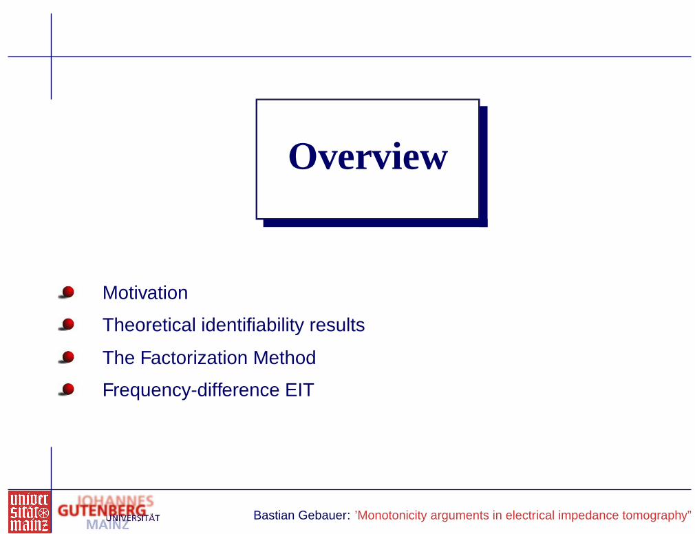
Overview
Motivation
Theoretical identifiability results
The Factorization Method
Frequency-difference EIT
Bastian Gebauer: ’Monotonicity arguments in electrical impedance tomography”

Motivation
Bastian Gebauer: ’Monotonicity arguments in electrical impedance tomography”

Electrical impedance tomography
(Images taken from EIT group at Oxford Brookes University,published in Wikipedia by William Lionheart)
Apply one or several input currents to a body and measure theresulting voltages
Goal: Obtain an image of the interior conductivity distribution.
Possible advantages:
EIT may be less harmful than other tomography techniques,
Conductivity contrast is high in many medical applications
Bastian Gebauer: ’Monotonicity arguments in electrical impedance tomography”

Electrical impedance tomography
Simple mathematical model for EIT:
S
BB: bounded domain
S ⊆ ∂B: relatively open subsetσ: electrical conductivity in B
g: applied current on S
Electric potential u that solves
∇ · σ∇u = 0, σ∂νu|∂B =
g on S,
0 else.
Direct Problem: (Standard theory of elliptic PDEs):For all σ ∈ L∞
+ (B), g ∈ L2⋄(∂B) there exists a unique solution u ∈ H1
⋄ (B).
Inverse Problems of EIT:How can we reconstruct (properties of) σ from measuring u|S ∈ L2
⋄(S)
for one or several input currents g?
Bastian Gebauer: ’Monotonicity arguments in electrical impedance tomography”
Identifiability results
Bastian Gebauer: ’Monotonicity arguments in electrical impedance tomography”

Regularity assumptions onσ
Most general, "natural" assumption: σ ∈ L∞+ (B).
Slightly less general:
σ ∈ L∞+ (B) and σ satisfies (UCP) in conn. neighborhoods U of S,
∇ · σ∇u = 0 and
u|S = 0, σ∂νu|S = 0 =⇒ u = 0.
u|V = const., V ⊂ U open =⇒ u = const.
For B ⊂ R2, (UCP) is satisfied for all σ ∈ L∞+ (B).
For B ⊂ Rn, n ≥ 3, (UCP) is satisfied, e.g., for Lipschitz continuous σ.
For σ ∈ C2(B), the EIT equation can be transformed to theSchrödinger equation
(∆ − q)u = 0 with q =∆√
σ√σ
"Strongest" regularity assumption: σ analytic or piecewise analytic
Bastian Gebauer: ’Monotonicity arguments in electrical impedance tomography”
Identifiability results
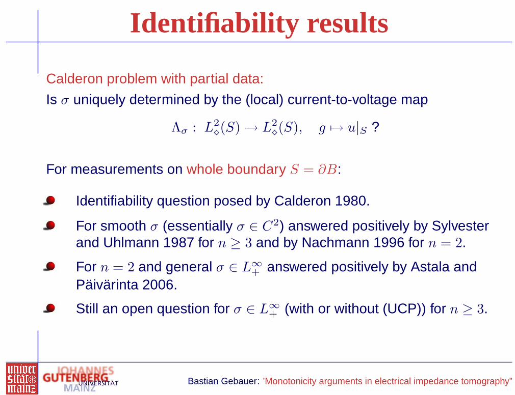
Calderon problem with partial data:
Is σ uniquely determined by the (local) current-to-voltage map
Λσ : L2⋄(S) → L2
⋄(S), g 7→ u|S ?
For measurements on whole boundary S = ∂B:
Identifiability question posed by Calderon 1980.
For smooth σ (essentially σ ∈ C2) answered positively by Sylvesterand Uhlmann 1987 for n ≥ 3 and by Nachmann 1996 for n = 2.
For n = 2 and general σ ∈ L∞+ answered positively by Astala and
Päivärinta 2006.
Still an open question for σ ∈ L∞+ (with or without (UCP)) for n ≥ 3.
Bastian Gebauer: ’Monotonicity arguments in electrical impedance tomography”
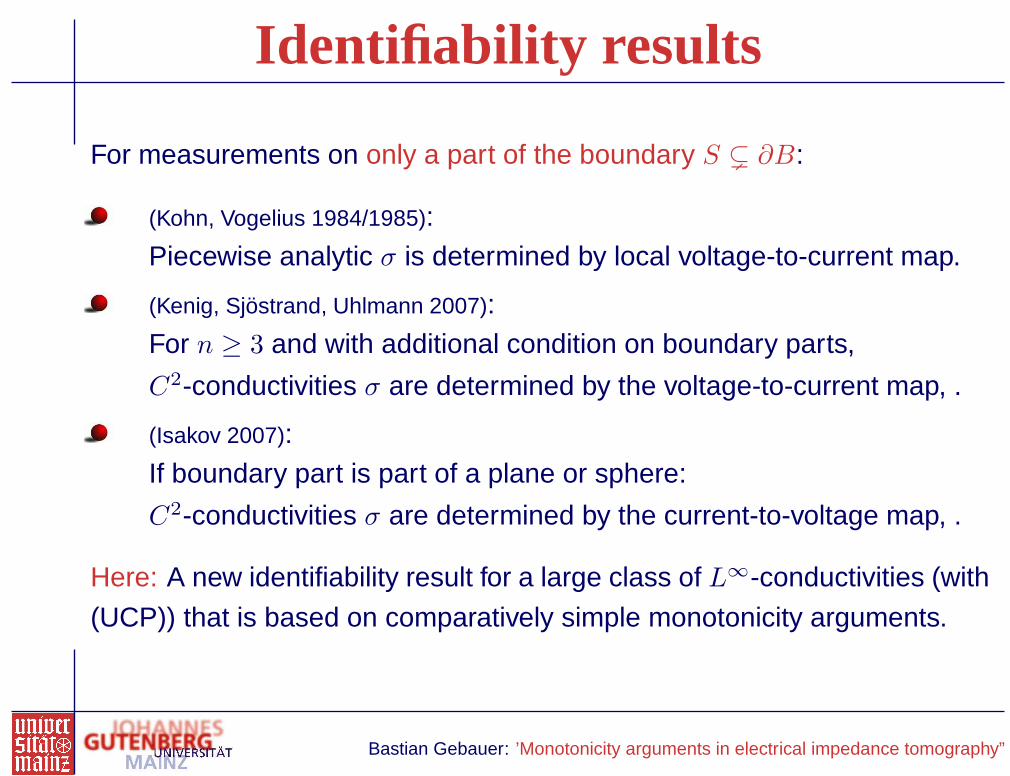
Identifiability results
For measurements on only a part of the boundary S ( ∂B:
(Kohn, Vogelius 1984/1985):Piecewise analytic σ is determined by local voltage-to-current map.
(Kenig, Sjostrand, Uhlmann 2007):For n ≥ 3 and with additional condition on boundary parts,
C2-conductivities σ are determined by the voltage-to-current map, .
(Isakov 2007):If boundary part is part of a plane or sphere:
C2-conductivities σ are determined by the current-to-voltage map, .
Here: A new identifiability result for a large class of L∞-conductivities (with
(UCP)) that is based on comparatively simple monotonicity arguments.
Bastian Gebauer: ’Monotonicity arguments in electrical impedance tomography”

Virtual Measurements
S
Ω
LΩ
f ∈ (H1⋄ (Ω))′: applied source on Ω
LΩ : (H1⋄ (Ω))′ → L2
⋄(S), f 7→ u|S ,
where u ∈ H1⋄ (B) solves
∫
B
σ∇u · ∇v dx = 〈f, v|Ω〉 for all v ∈ H1⋄ (B).
If Ω ⊂ B: ∆u = fχΩ, σ∂νu|∂B = 0.
(UCP) yields: If Ω1 ∩ Ω2 = ∅, B \ (Ω1 ∪ Ω2) is connected and its boundarycontains S then R(LΩ1
) ∩R(LΩ2) = 0.
Dual operator L′Ω : L2
⋄(S) → H1⋄ (Ω), g 7→ u|Ω, where u solves
∇ · σ∇u = 0, σ∂νu|∂B =
g on S,
0 else.
Bastian Gebauer: ’Monotonicity arguments in electrical impedance tomography”
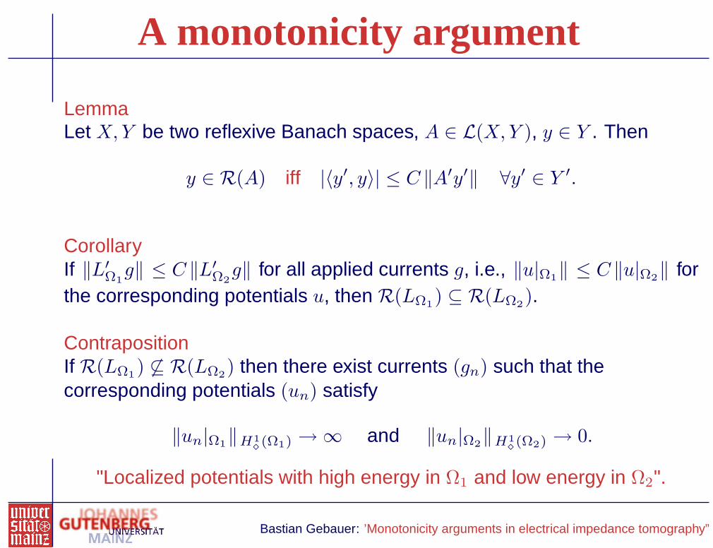
A monotonicity argument
LemmaLet X, Y be two reflexive Banach spaces, A ∈ L(X, Y ), y ∈ Y . Then
y ∈ R(A) iff |〈y′, y〉| ≤ C ‖A′y′‖ ∀y′ ∈ Y ′.
CorollaryIf ‖L′
Ω1g‖ ≤ C ‖L′
Ω2g‖ for all applied currents g, i.e., ‖u|Ω1
‖ ≤ C ‖u|Ω2‖ for
the corresponding potentials u, then R(LΩ1) ⊆ R(LΩ2
).
ContrapositionIf R(LΩ1
) 6⊆ R(LΩ2) then there exist currents (gn) such that the
corresponding potentials (un) satisfy
‖un|Ω1‖H1
⋄(Ω1) → ∞ and ‖un|Ω2
‖H1⋄(Ω2) → 0.
"Localized potentials with high energy in Ω1 and low energy in Ω2".
Bastian Gebauer: ’Monotonicity arguments in electrical impedance tomography”
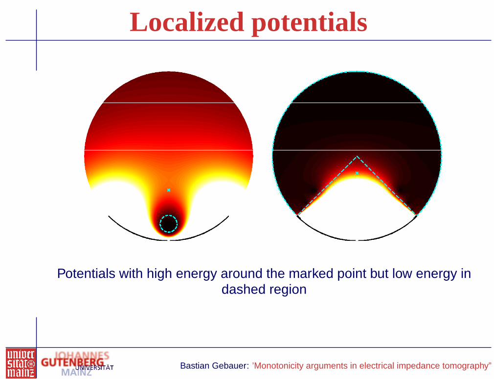
Localized potentials
Potentials with high energy around the marked point but low energy indashed region
Bastian Gebauer: ’Monotonicity arguments in electrical impedance tomography”
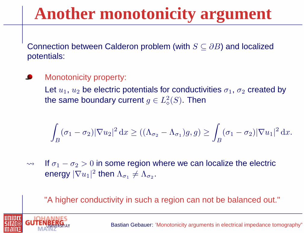
Another monotonicity argument
Connection between Calderon problem (with S ⊆ ∂B) and localizedpotentials:
Monotonicity property:
Let u1, u2 be electric potentials for conductivities σ1, σ2 created bythe same boundary current g ∈ L2
⋄(S). Then
∫
B
(σ1 − σ2)|∇u2|2 dx ≥ ((Λσ2− Λσ1
)g, g) ≥∫
B
(σ1 − σ2)|∇u1|2 dx.
If σ1 − σ2 > 0 in some region where we can localize the electricenergy |∇u1|2 then Λσ1
6= Λσ2.
"A higher conductivity in such a region can not be balanced out."
Bastian Gebauer: ’Monotonicity arguments in electrical impedance tomography”

A new identifiability result
Theorem (G, 2008)
Let σ1, σ2 ∈ L∞+ (B) satisfy (UCP) and Λσ1
, Λσ2be the corresponding
current-to-voltage-maps.
If σ2 ≥ σ1 in some neighborhood V of S and σ2 − σ1 ∈ L∞+ (U) for some
open U ⊆ V then there exists (gn) such that
〈(Λσ2− Λσ1
)gn, gn〉 → ∞,
so in particular Λσ26= Λσ1
.U
V
Two conductivities can be distinguished if one is larger in some part thatcan be connected to the boundary without crossing a sign change.
Bastian Gebauer: ’Monotonicity arguments in electrical impedance tomography”

Remarks
Remarks
Theorem covers the Kohn-Vogelius result:
σ|S and its derivatives on S are uniquely determined by Λσ.
Piecewise analytic conductivities σ are uniquely determined.
Theorem holds for general L∞+ -conductivities with (UCP).
(In particular, it is not covered by the recent result of Isakov.)
Theorem uses only monotonicity properties of real elliptic PDEs, thusalso holds e.g. for linear elasticity, electro- and magnetostatics.
However,
Theorem needs a neighborhood without sign change. It cannotdistinguish infinitely fast oscillating C∞-conductivities from constantones.The identifiability question for general L∞
+ -conductivities (with orwithout (UCP)) for n ≥ 3 or partial boundary data is still open.
Bastian Gebauer: ’Monotonicity arguments in electrical impedance tomography”
The Factorization Method
Bastian Gebauer: ’Monotonicity arguments in electrical impedance tomography”

Detecting inclusions in EITSpecial case of EIT: locate inclusions in known background medium.
Ω
S
Current-to-voltage map with inclusion:
Λ1 : g 7→ u1|∂B ,
where u1 solves
∇ · σ∇u1 = 0 ∂νu1|∂B =
g on S,
0 else,
with σ = 1 + σ1χΩ, σ1 ∈ L∞+ (Ω).
S
Current-to-voltage map without inclusion:
Λ0 : g 7→ u0|∂B ,
where u0 solves the analogous equationwith σ = 1.
Goal: Reconstruct Ω from comparing Λ1 with Λ0.
Bastian Gebauer: ’Monotonicity arguments in electrical impedance tomography”
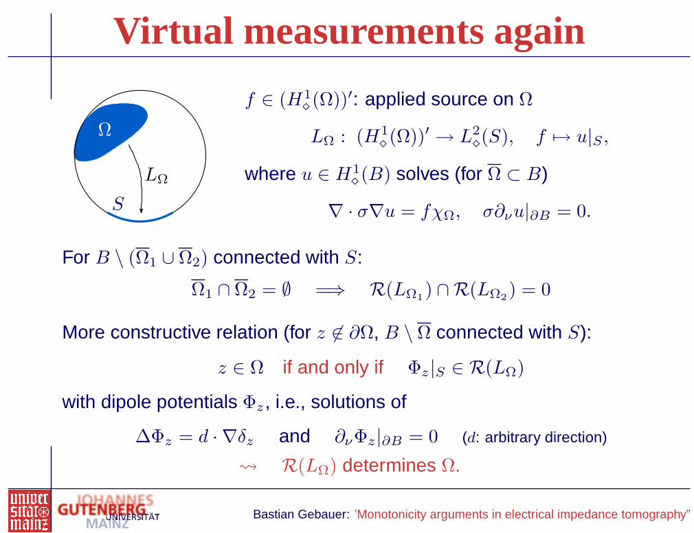
Virtual measurements again
S
Ω
LΩ
f ∈ (H1⋄ (Ω))′: applied source on Ω
LΩ : (H1⋄ (Ω))′ → L2
⋄(S), f 7→ u|S ,
where u ∈ H1⋄ (B) solves (for Ω ⊂ B)
∇ · σ∇u = fχΩ, σ∂νu|∂B = 0.
For B \ (Ω1 ∪ Ω2) connected with S:
Ω1 ∩ Ω2 = ∅ =⇒ R(LΩ1) ∩ R(LΩ2
) = 0
More constructive relation (for z 6∈ ∂Ω, B \ Ω connected with S):
z ∈ Ω if and only if Φz|S ∈ R(LΩ)
with dipole potentials Φz, i.e., solutions of
∆Φz = d · ∇δz and ∂νΦz|∂B = 0 (d: arbitrary direction)
R(LΩ) determines Ω.
Bastian Gebauer: ’Monotonicity arguments in electrical impedance tomography”
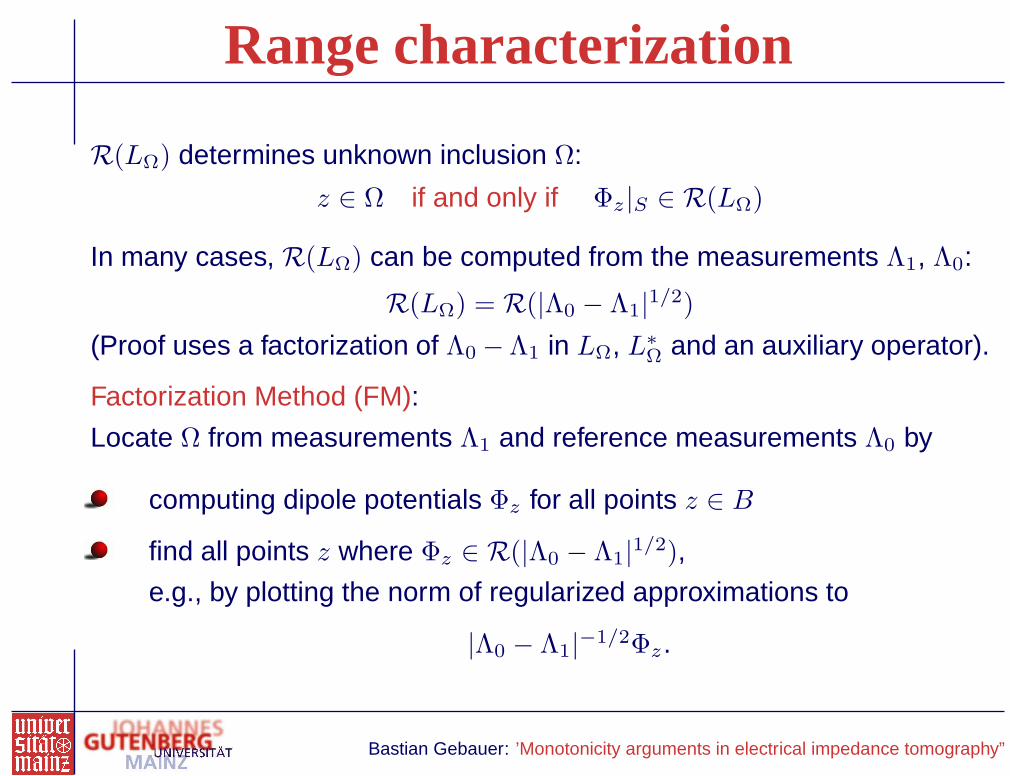
Range characterization
R(LΩ) determines unknown inclusion Ω:
z ∈ Ω if and only if Φz|S ∈ R(LΩ)
In many cases, R(LΩ) can be computed from the measurements Λ1, Λ0:
R(LΩ) = R(|Λ0 − Λ1|1/2)
(Proof uses a factorization of Λ0 −Λ1 in LΩ, L∗Ω and an auxiliary operator).
Factorization Method (FM):
Locate Ω from measurements Λ1 and reference measurements Λ0 by
computing dipole potentials Φz for all points z ∈ B
find all points z where Φz ∈ R(|Λ0 − Λ1|1/2),
e.g., by plotting the norm of regularized approximations to
|Λ0 − Λ1|−1/2Φz.
Bastian Gebauer: ’Monotonicity arguments in electrical impedance tomography”

History and known results
FM relies on range identity like R(LΩ) = R(|Λ0 − Λ1|1/2).
FM originally developed by Kirsch for inverse scattering problemsand extended to different settings and boundary conditions(with Arens, Grinberg)
FM generalized to EIT (Brühl/Hanke, 1999)
FM extended to many applications including electrostatics (Hähner),EIT with electrode models (Hyvönen, Hakula, Pursiainen, Lechleiter),EIT in half-space (Schappel),harmonic vector fields (Kress), Stokes equations (Tsiporin),optical tomography (Hyvönen, Bal, G), linear elasticity (Kirsch),general real elliptic problems (G),parabolic-elliptic problems (Frühauf, G, Scherzer)
All these results rely on a parameter jump.Can FM also detect smooth transitions from background to inclusion?
Bastian Gebauer: ’Monotonicity arguments in electrical impedance tomography”

Monotonicity arguments
Λ1: NtD for σ = 1 + σ1χΩ1, Λ2: NtD for σ = 1 + σ2χΩ2
, σ1, σ2 ≥ 0
Monotony between conductivity and measurements (NtDs):
σ1χΩ1≤ σ2χΩ2
=⇒ (Λ1g, g) ≥ (Λ2g, g) for all g ∈ L2⋄(S)
Together with range monotony:
σ1χΩ1≤ σ2χΩ2
=⇒ R((Λ0 − Λ1)1/2) ⊆ R((Λ0 − Λ2)
1/2)
Result of range tests Φz ∈ R((Λ0 − Λ1)1/2) is monotonous w.r.t. the
inclusions size and contrast.
FM-theory can be extended to irregular inclusions (e.g. with smoothtransitions) by estimating them from above and below by regularinclusions with sharp jumps.
Bastian Gebauer: ’Monotonicity arguments in electrical impedance tomography”

FM with irregular inclusions
Λ1: NtD for σ = 1 + σ1χΩ1, Λ0: NtD for σ = 1.
Theorem (G, Hyvonen 2007)
Let σ1 ≥ 0 and Ω have a connected complement.
Φz ∈ R((Λ0 − Λ1)1/2) for every z ∈ Ω for which σ1 is locally in L∞
+ .
Φz 6∈ R((Λ0 − Λ1)1/2) for every z 6∈ Ω.
(and an analogous results holds for σ1 ≤ 0.)
FM does not only find inclusions where a parameter “jumps”,but also where it merely “differs” from a known background value.
Bastian Gebauer: ’Monotonicity arguments in electrical impedance tomography”

Numerical example
real conductivity “‖|Λ0 − Λ1|−1/2Φz‖ ” contour lines
Numerical results for inclusions with smooth transitions in EIT
Bastian Gebauer: ’Monotonicity arguments in electrical impedance tomography”

Numerical example
real conductivity “‖|Λ0 − Λ1|−1/2Φz‖ ” contour lines
Numerical results with 0.1% noise
Bastian Gebauer: ’Monotonicity arguments in electrical impedance tomography”

Remarks
Remarks
Using monotonicity arguments the assumptions of the FactorizationMethod can be reduced to local properties.
FM also works for inclusions that are not sharply separated from thebackground.
With the same technique one can eliminate boundary regularityassumptions, or simultaneously treat inclusions of different types(e.g. absorbing and conducting, G and Hyvönen 2008).
However,
The result still needs a global definiteness property (σ1 ≥ 0 or σ1 ≤ 0in all inclusions). FM for indefinite problems is still an open problem.
Bastian Gebauer: ’Monotonicity arguments in electrical impedance tomography”

Frequency-difference EIT
Bastian Gebauer: ’Monotonicity arguments in electrical impedance tomography”

Reference measurements
Factorization method uses difference Λ1 − Λ0 between
actual measurements Λ1
reference measurements Λ0 at an inclusion-free body
Advantage: If reference measurements are available then systematicerrors cancel out, e.g., forward modeling errors about the bodygeometry.
Disadvantage: If reference measurements have to be simulated (orcalculated analytically) then forward modeling errors have a largeimpact on the reconstructions.
In medical application, reference measurements at an inclusion-freebody are usually not available.
Bastian Gebauer: ’Monotonicity arguments in electrical impedance tomography”
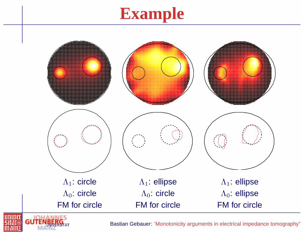
Example
Λ1: circle Λ1: ellipse Λ1: ellipseΛ0: circle Λ0: circle Λ0: ellipse
FM for circle FM for circle FM for circle
Bastian Gebauer: ’Monotonicity arguments in electrical impedance tomography”
Possible solution
Possible solution: Replace reference measurements bymeasurements at another frequency.
Frequency-dependent EIT:
g: applied current, time-harmonic with frequency ω
electric potential uω that solves
∇ · γω∇uω = 0, γω∂νuω|∂B =
g on S,
0 else.
with complex conductivity γω = σ + iǫω , ǫ: dielectricity.
Measurements at frequency ω Current-to-voltage (NtD) map
Λω : g 7→ uω|S
Bastian Gebauer: ’Monotonicity arguments in electrical impedance tomography”

Sketch of the idea
How to use frequency-difference measurements:
Given two frequ. ω, τ > 0, conductivities γω, γτ and NtDs Λω, Λτ
Assume that for all x outside the inclusion Ω
γω(x) = γω0 ∈ C and γτ (x) = γτ
0 ∈ C
Using γω0 Λω and γτ
0 Λτ scales down conductivity outside Ω to 1.
Difference γω0 Λω − γτ
0 Λτ should have similar properties to Λ1 − Λ0.
FM should also work with γω0 Λω − γτ
0 Λτ instead of Λ1 − Λ0.
For non-zero frequencies, γω0 Λω is not self-adjoint, so we will have to
use its real or imaginary part
ℑ(A) := 12i (A − A∗), ℜ(A) := 1
2 (A + A∗)
for an operator A : L2⋄(S) → L2
⋄(S).
Bastian Gebauer: ’Monotonicity arguments in electrical impedance tomography”
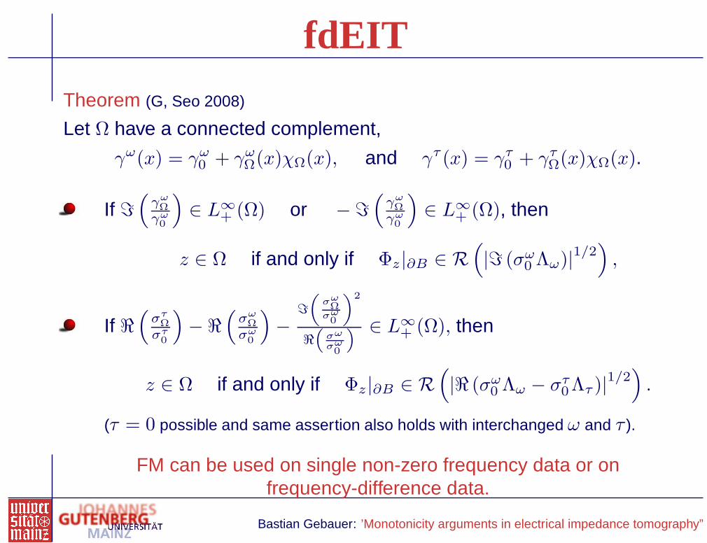
fdEIT
Theorem (G, Seo 2008)
Let Ω have a connected complement,
γω(x) = γω0 + γω
Ω(x)χΩ(x), and γτ (x) = γτ0 + γτ
Ω(x)χΩ(x).
If ℑ(
γω
Ω
γω
0
)
∈ L∞+ (Ω) or − ℑ
(
γω
Ω
γω
0
)
∈ L∞+ (Ω), then
z ∈ Ω if and only if Φz|∂B ∈ R(
|ℑ (σω0 Λω)|1/2
)
,
If ℜ(
στ
Ω
στ
0
)
−ℜ(
σω
Ω
σω
0
)
−ℑ
„
σω
Ω
σω
0
«
2
ℜ
“
σω
σω
0
” ∈ L∞+ (Ω), then
z ∈ Ω if and only if Φz|∂B ∈ R(
|ℜ (σω0 Λω − στ
0Λτ )|1/2)
.
(τ = 0 possible and same assertion also holds with interchanged ω and τ ).
FM can be used on single non-zero frequency data or onfrequency-difference data.
Bastian Gebauer: ’Monotonicity arguments in electrical impedance tomography”
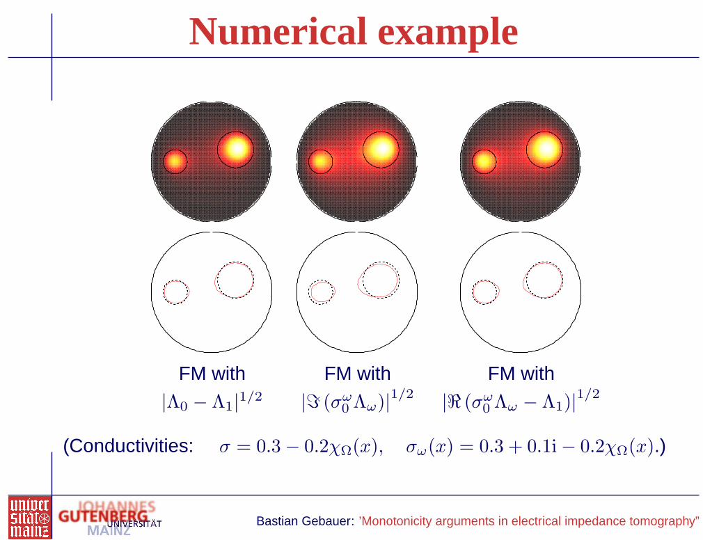
Numerical example
FM with FM with FM with
|Λ0 − Λ1|1/2 |ℑ (σω0 Λω)|1/2 |ℜ (σω
0 Λω − Λ1)|1/2
(Conductivities: σ = 0.3 − 0.2χΩ(x), σω(x) = 0.3 + 0.1i − 0.2χΩ(x).)
Bastian Gebauer: ’Monotonicity arguments in electrical impedance tomography”

Numerical example
|Λcirc0 − Λ1|
1
2 |Λellipse0 − Λ1|
1
2 |ℜ (σω0 Λω − Λ1)|
1
2 |ℑ (σω0 Λω)| 12
Reconstructions of an ellipse-shaped body that is wrongly assumed to be a circle.
Bastian Gebauer: ’Monotonicity arguments in electrical impedance tomography”
Unknown background
FM for frequency-difference EIT requires no reference data but stillneeds to know the constant background conductivity
Heuristic method to estimate this from the data:Eigenvectors for low eigenvalues should belong to highlyoscillating potentials that do not penetrate deeply.
Most of the quotients of eigenvalues of Λω and Λτ should behavelike γτ
0 /γω0 .
For zero-frequency data Λτ = Λ1 we use |ℜ (αΛω − Λ1)|1
2 withthe median α of quotients of eigenvalues of Λω and Λ1.
Analogously, the phase of γω0 can be estimated from quotients of
real and imaginary part of the eigenvalues of Λω.
Bastian Gebauer: ’Monotonicity arguments in electrical impedance tomography”

Unknown background
no noise 0.1% noise
Reconstructions for unknown background conductivity without and with noise.
Bastian Gebauer: ’Monotonicity arguments in electrical impedance tomography”

Remarks
Remarks
Simulating reference data makes Factorization Method vulnerable toforward modeling errors.
Using frequency-difference measurements strongly improves FMsrobustness. Results are comparable to those with correct referencedata.
Unknown background conductivities can be estimated from the data.
However,
Scaling the conductivity by simple multiplication only works forconstant background conductivity.
Theory needs contrast conditions in the inclusions with globaldefiniteness properties.
Bastian Gebauer: ’Monotonicity arguments in electrical impedance tomography”

Conclusions
Comparatively simple monotony arguments yield :
New theoretical identifiability result for the Calderon-problem
Two conductivities can be distinguished if one is larger in somepart that can be connected to the boundary without crossing asign change.
Improvements for the Factorization Method:
FM does not only find inclusions where a parameter “jumps”, butalso where it merely “differs” from a known background value.
Reference data can be replaced by frequency-difference data,thus strongly improving the methods robustness.
However,
There are important open problems connected with definitenessproperties.
Bastian Gebauer: ’Monotonicity arguments in electrical impedance tomography”