Monotone Method for Finite Difference Equations Of ... · corresponds to the nonlinear reaction diffusion equations with linear ... first developed this method for nonlinear parabolic

International Journal of Universal Mathematics and Mathematical Sciences

ISSN: 2454-7271 Volume: 02, Issue: 01, Pages:01-13,

Published:June,2016 Web: www.universalprint.org ,

Title Key: Monotone Method For Finite Difference Equations…

R. M. Dhaigude Page 1

Monotone Method for Finite Difference Equations

Of Reaction Diffusion and Applications

R. M. Dhaigude Department of Mathematics,

Government Vidarbha Institute of Science and Humanities, Amaravati- 444 604 (M. S.) INDIA.

Email : [email protected]

Abstract

The purpose of this paper is to develop monotone iteration scheme using the notion

of upper and lower solutions of nonlinear finite difference equations,which

corresponds to the nonlinear reaction diffusion equations with linear boundary

conditions. Two monotone sequences are constructed for the finite difference

equations when two sequences converge monotonically from above and below to

maximal and minimal solutions, which leads to the Existence-Comparison and

Uniqueness results for the solution of the nonlinear finite difference system.

Positivity Lemma is the main ingredient used in the proof of these results.

Keywords : Monotone Scheme, Monotone Property, Existence-Comparison

Theorem, Uniqueness Theorem.

Mathematics Subject Classification : Ams: 65 No 5; CR; G 1.8

1. Introduction

Various real problems in different fields from science and technology are governed

by nonlinear reaction diffusion equations. The method of upper and lower solutions

is one of the well known method employed successfully in the study of existence-

comparison and uniqueness of solutions of IBVP of a nonlinear partial differential

equations. In 1992,Sattinger [8] first developed this method for nonlinear parabolic

as well as elliptic boundary value problems. An excellent account of these results are

given in the elegant books by Ladde, Lakshmikantham and Vatsala [5] and Pao [7].

In the year 1985, Pao [6] developed this method for finite difference equations of

nonlinear parabolic and elliptic boundary value problems. Here, we develop the

http://www.universalprint.org/

mailto:[email protected]






monotone scheme for finite difference system of nonlinear time degenerate parabolic

problems.

We plan the paper as follows:

In section 2, finite difference system of nonlinear time degenerate parabolic initial

boundary value problem is formulated from the corresponding continuous problem

under consideration. Section 3 is devoted for the monotone scheme for the discrete

problem. Using upper and lower solutions as distinct initial iterations, two

monotone sequences are constructed, which converge monotonically from above

and below to maximal and minimal solutions respectively. Also the existence-

comparison and uniqueness results for discrete problems are discussed in the last

section.

2. Finite Difference Equations:

Consider the time degenerate Dirichlet initial boundary value problem

d(x, t)ut – L[u] = f(x, t, u); in DT

Boundary condition u(x, t) = h(x, t ); on ST (2.1)

Initial condition u(x, 0) = ψ(x); in Ω

This equation can be written as

d(x, t)ut – L[u] + c(x, t)u = c(x, t)u + f(x, t, u); in DT

u(x, t) +b (x,t)u= b (x,t)u +h(x, t ); on ST (2.2)

u(x, 0) = ψ(x); in Ω

where Ω is a bounded domain in IRP (P = 1, 2, ……..)with boundary Ω; DT , ST ,

T > 0, L[u] =2n n

i. j j

ij 1 j 1i j j

u ua (x, t) b (x, t)

k k x

i.e. L[u] = D(x, t) 2u + b(x, t) . u and

b(x, t) . u = b(1)(x,t) (p)

1 p

u u...... b (x, t) .

x x

Note that D(x, t) > 0 and b(x, t) are diffusion and convection coefficients respectively

on DT. Now, we write the discrete version of the above continuous time degenerate

Dirichlet IBVP (2.1) by converting it into finite difference equations.

Suppose that i = (i1, i2, i3,… iP) is a multiple index with iv = 0, 1, 2,., Mv + 1 and xi

= (xi1, xi2, ., xip) is a arbitrary mesh point in Ωp where Mv is the total number of

interior mesh points in the xiv coordinate direction. Denote by Ωp, p, Ωp, Λp and

Sp the sets of mesh points in Ω, , Ω, and ; DT , ST respectively and .p ,denote the

set of all mesh points. Suppose (i, n) is used to represent the mesh point (xi, tn).







Set ui,n u(xi, tn); fi,n(ui,n) f(xi, tn, u(xi, tn)); gi,n(ui,n) g(xi, tn, u(xi, tn));

Di,n D(xi, tn) bi,n b(xi, tn); ψi ψ(xi); ui,0 u(xi,0); di,n d(xi, tn).

Suppose kn = tn – tn – 1 is the nth time increment for n = 1, 2, …..,N and hv is the special

increment in the xiv coordinate direction. Suppose Cv = (0, …… 1, …….0) is the unit

vector in Rp where the constant 1 appears in the vth component and zero elsewhere.

Using the standard second order difference approximations. We have vui,n = hv–2 [u(xi + hvev, tn) – 2u(xi, tn) + u(xi – hvev, tn)]

Also we have the standard forward and backward first order difference

approximations

+(v) ui,n = hv–1 [u(xi + hvev, tn) – u(xi, tn)] and

–(v) ui,n = hv–1 [u(xi,tn ) – u(xi – hvev, tn)] respectively.

In order to avoid the technical difficulties construction of monotone sequences,

suppose that each component bl(xi, tn), l = 1, 2, ….., p has the same sign in Ωp but

boundary difference possess different signs for different .Then we can define the

first order approximations in the Xiv coordinate direction as ( ) ( )

, ,( )

, ( ) ( )

, ,

when 0

when 0

v v

i n i nv

i n v v

i n i n

u bu

u b

Now the discrete version of the continuous problem

(2.1) is given by

£ [ui,n] di,nkn–1 (ui,n – ui,n –1) – L[ui,n] = fi,n(ui,n); (i, n) p. (2.3)

ui,n = gi,n(ui,n); (i, n) Sp

ui,0 = ψi; i Ωp

This problem (2.3) can be written as

di,nkn–1 (ui,n – ui,n – 1) – L[ui,n] + ci,nui,n = ci,nui,n + fi,n(ui,n); in p

ui,n + bi,nui,n = bi,nui,n + gi,n(ui,n); (i,n) Sp (2.4)

ui,0 = ψi; i Ωpc where ( ) ( ) ( )

, , , , ,

1

[ ] ( ).p

v v v

i n i n i n i n i n

v

L u D u b u

Assume that

(i) The coefficient di,n is a non-negative in p. However we will not assume that di,n

is a bounded away from zero. Since di,n = 0 for some (i, n) p and hence the

equation is time degenerate,

(ii) The functions fi,n(ui,n); gi,n(ui,n), ψi and ui,n are Holder continuous functions in

their respective domains,







(iii) fi,n(ui,n) and gi,n(ui,n) satisfies the Lipschitz condition ui,n in p (1) (2) (1) (2) (1) (2)

, , , , , , , , , ,

(1) (2) (1) (2) (1) (2)

, , , , , , , , , ,

i n i n i n i n i n i n i n i n i n i n

i n i n i n i n i n i n i n i n i n i n

c u u f u f u c u u

b u u g u g u b u ufor (2) (1)

, , , ,ˆ ,i n i n i n i nu u u u

(iv) Fi,n(ui,n) ci,nui,n + fi,n(ui,n) is a monotone nondecreasing in ui,n for , , ,ˆ

i n i n i nu u u

and satisfies the Lipschitz condition (1) (2) (1) (1) (2) (1) (2)

, , , , , , , , , , ,ˆ| | for , , .i n i n i n i n i n i n i n i n i n i n i nF u F u k u u u u u u

where (1)

,i nk is a constant and independent of (i, n),

(v) The function Gi,n(ui,n) = bi,nui,n + gi,n(ui,n) is a monotone nondecreasing in ui,n, for

, , ,ˆ ,i n i n i nu u u and satisfies the Lipschitz condition

(1) (2) (2) (1) (2) (1) (2)

, , , , , , , , , , ,ˆ| | For , , .i n i n i n i n i n i n i n i n i n i n i nG u G u K u u u u u u

In terms of F and G the problem (2.4)

can be written as

£[ui,n] = Fi,n(ui,n); (i, n) p

ui,n + bi,nui,n = hi,n(ui,n); (i, n) Sp (2.5)

ui,0 = ψi; i Ωp

where £[ui,n] di,nkn–1[ui,n – ui,n–1] – L[ui,n] + ci,nui,n.

The system (2.3) gives a suitable finite difference approximation for the construction

of monotone sequences.

To prove our main results we develop monotone scheme for the finite

difference equation (2.2). The following positivity lemma is a discrete version of the

positivity lemma for the continuous problem.

Lemma 2.1 (Positivity Lemma) Suppose that ui,n satisfies the following inequalities

di,nkn–1 (ui,n – ui,n –1) – L[ui,n] + ci,nui,n ≥ 0 in p

Bui,n (xi, tn)|xi – x i|–1 [u(xi,tn) – u( x I, tn)] + i,nui,n ≥ 0 on Sp (2.6)

ui,0 ≥ 0 in Ω

where ci,n ≥ 0; di,n ≥ 0; x i is a suitable point in Ωp and |xi – x i| is the distance between

xi and x i . i,n ≥ 0; i,n ≥ 0; i,n + i,n > 0; on Sp and c ci,n is a bounded function in p.

Then ui,n ≥ 0 in p. Moreover ui,n > 0 in p, unless it is identically zero.

Proof is simple so details are omitted.

3. Monotone Scheme







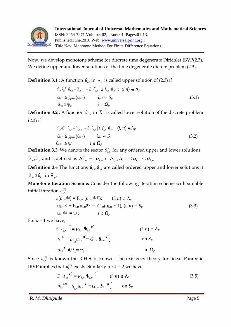
Now, we develop monotone scheme for discrete time degenerate Dirichlet IBVP(2.3).

We define upper and lower solutions of the time degenerate dicrete problem (2.3).

Definition 3.1 : A function ,i nu in p is called upper solution of (2.3) if

1

, , , 1 , , , ;i n n i n i n i n i n i nd k u u L u f u (i,n) p

ũi,n ≥ gi,n (ũi,n) i,n Sp (3.1)

,0 ,i iu i Ωp

Definition 3.2 : A function ,ˆ

i nu in p is called lower solution of the discrete problem

(2.3) if 1

, , , 1 , , ,ˆ ˆ ˆ ˆ ;i n n i n i n i n i n i nd k u u L u f u (i, n) p

ûi,n ≤ gi,n (ûi,n) i,n Sp (3.2)

ûi,0 ≤ ψi i Ωp

Definition 3.3: We denote the sector *

,i nS for any ordered upper and lower solutions

, ,ˆ,i n i nu u and is defined as *

, , , , ,ˆ;i n i n p i n i n i nS u u u u

Definition 3.4 The functions , ,ˆ,i n i nu u are called ordered upper and lower solutions if

, ,ˆ

i n i nu u in .p

Monotone Iteration Scheme: Consider the following iteration scheme with suitable

initial iteration (0)

. ,i nu

£[ui,n(k)] = Fi,n (ui,n (k-1)); (i, n) p

ui,n(k) + bi,n ui,n(k) = Gi,n(ui,n (k-1) ); (i, n) Sp (3.3)

ui,0(k) = ψi; i Ωp

For k = 1 we have,

£ 0

,,

1

, ninini uFu (i, n) p

0,,

1,

,

)1(

, uGubu ninininini on Sp

ii xu 0,1

0, in Ωp

Since (0)

,i nu is known the R.H.S. is known. The existency theory for linear Parabolic

IBVP implies that (2)

,i nu exists. Similarly for k = 2 we have

£ 1

,,

2

, ninini uFu (i, n) p (3.5)

1,,

2,

,

)2(

, uGubu ninininini on Sp







ii xu 0,

2

0, in Ωp

Since 1,u ni is known the R.H.S. is known. The existence theory for linear Parabolic

IBVPs implies that 2,u ni exists. Thus for k = 3, 4, ……… we get (3) (4)

, ,, ,.....i n i nu u

Thus we construct a sequence, the sequence is well defined follows from Lemma 2.1.

We choose initial iteration (0)

, ,i n i nu u and denote the sequence by ( )

, .k

i nu We also

choose initial iteration (0)

, ,i n i nu u and denote the sequence by ( )

, .k

i nu Thus choosing an

upper solution or lower solution as the initial iterations, we get upper and lower

sequences ( ) ( )

, ,andk k

i n i nu u respectively.

Lemma 3.1 (Monotone Property) : Suppose that

(i) , ,ˆ,i n i nu u are ordered upper and lower solutions of nonlinear time degenerate

Dirichlet IBVP (2.3),i.e.

di,n1

nk [ui,n – ui,n–1] – L[ui,n] = fi,n(ui,n); in p

ui,n = gi,n(ui,n); on Sp

ui,0 = ψi; i Ωp,

(ii) fi,n(ui,n) and gi,n(ui,n) satisfies the Lipschitz condition (1) (2) (1) (2) (1) (2)

, , , , , , , , , ,i n i n i n i n i n i n i n i n i n i nc u u f u f u c u u

(1) (2) (1) (2) (1) (2)

, , , , , , , , , ,i n i n i n i n i n i n i n i n i n i nb u u g u g u b u u (3.6)

for (1) (2)

, , , ,ˆ, , .i n i n i n i nu u u u Then the sequences ( ) ( )

, ,,k k

i n i nu u possess the monotone

property.

( ) ( 1) ( 1) ( )

, , , , , ,ˆ k k k k

i n i n i n i n i n i nu u u u u u in .p (3.7)

Moreover, ( ) ( )

, ,andk k

i n i nu u are ordered upper and lower solutions of time degenerate

Dirichlet IBVP for k = 1, 2, 3, ……

Proof: Define

(0) (1)

, , ,i n i n i nw u u

(1)

, , , .i n i n i nw u u (0)

, ,i n i nu u

Since ,i nu is an upper solution, we have by definition 3.1 1

, , , 1 , , , ;i n n i n i n i n i n i nd k u u L u f u in p

ũi,n ≥ gi,n (ũi,n) i,n Sp

,0 ,i iu i Ωp,







Clearly

1 1 1 (1) (1)

, , , 1 , , , 1 , , , 1[ ]i n n i n i n i n n i n i n i n m i n i nd k w w d k u u d k u u

(1)

, , ,[ ]i n i n i nL w L u L u

(1)

, , , , , , .i n i n i n i n i n i nc w c u c u

By adding we get 1

, , , 1 , , ,[ ]i n n i n i n i n i n i nd k w w L w c w 1

, , , 1 , , ,[ ]i n n i n i n i n i n i nd k u u L u c u

1 (1) (1) (1) (1)

, , , 1 , , ,[ ]i n n i n i n i n i n i nd k u u L u c u

1 (0) (0)

, , , 1 , , , , , , ,[ ]i n n i n i n i n i n i n i n i n i n i nd k u u L u c u c u f u (By iterative scheme)

1

, , , 1 , , , , , , ,

1

, , , 1 , , ,

[ ] ( )

[ ] ( ) 0

i n n i n i n i n i n i n i n i n i n i n

i n n i n i n i n i n i n

d k u u L u c u c u f u

d k u u L u f u

1

, , , , , ,[ ] [ ] 0,i n n i n i n i n i n i nd k w w L w c w in p

Also, 0.,,, ninini wbw ; on Sp and

(1)

,0 ,0 ,0

,0 0

i i i

i i

w u u

u

wi,0 ≥ 0 in Ω

Now applying the Lemma 2.1 we get, wi,n ≥ 0; in p. This implies that

(1) (0)

, ,i n i nu u (3.8)

We also know that ,ˆ

i nu is a lower solution.

Define (1) (0)

, , ,i n i n i nw u u and using (0)

, ,ˆ ,i n i nu u We have (1)

, , ,ˆ ,i n i n i nw u u

using the above argument we get, (1) (0)

, , .i n i nu u (3.9)

Next we define (1) (1) (1)

, , ,i n i n i nw u u

1 (1) (1) (1) (1)

, , , 1 , , ,

1 (1) (1) (1) (1)

, , , 1 , , ,

1 (1) (1) (1) (1)

, , , 1 , , ,




d k w w L w c w

d k u u L u c u

d k u u L u c u

, , , ,ˆ 0.i n i n i n i nF u f u Also wi,n(1) +bi,nwi,n(1) ≥ 0 ;

(1) (1) (1)

,0 ,0 ,0i i iw u u = i – I = 0:

Applying the lemma 2.1 we get, (1)

,0 0iw . This shows that (1) (1)

,0 ,i i nu u (3.10)

we conclude that (0) (1) (1) (0)

, , , ,i n i n i n i nu u u u (3.11)

Assume by induction ( 1) ( ) ( ) ( 1)

, , , , in .k k k k

i n i n i n i n pu u u u (3.12)







Define function ( ) ( ) ( 1)

, , , .k k k

i n i n i nw u u

Using iterative scheme and Lipschitz condition, w(k) satisfies the relation

1 ( ) ( ) ( ) ( )

, , , 1 , , ,

k k k k

i n n i n i n i n i n i nd k w w L w c w 1 ( ) ( ) ( ) ( )

, , , 1 , , ,

k k k k

i n n i n i n i n i n i nd k u u L u c u

1 ( 1) ( 1) ( 1) ( 1)

, , , 1 , , ,

k k k k

i n n i n i n i n i n i nd k u u L u c u

( 1) ( 1) ( ) ( )

, , , , , , , ,

k k k k

i n i n i n i n i n i n i n i nc u f u c u f u

( 1) ( )

, , , , 0k k

i n i n i n i nF u F u

1 ( ) ( ) ( ) ( )

, , , 1 , , ,| 0 ink k k k

i n n i n i n i n i n i n pd k w w L w c w ;

Also wi,n(k)+bi,nwi,n(

( 1) ( )

, , , , 0k k

i n i n i n i nG u G u

(0) ( ) ( 1)

,0 ,0 ,0

k k

i i iw u u = i – i = 0 ( )

,0 0,k

iw in Ωp

Again applying the lemma 2.1 we get, ( )

,0 0k

iw ; i.e. ( 1) ( )

, ,

k k

i n i nu u (3.13)

Similarly consider ( ) ( 1) ( )

, , ,

k k k

i n i n i nw u u

1 ( ) ( ) ( ) ( )

, , , 1 , , ,

k k k k

i n n i n i n i n i n i nd k w w L w c w ( ) ( ) ( 1) ( 1)

, , , , , , , ,

k k k k


(By using iterative scheme and Lipschitz condition), 1 ( ) ( ) ( ) ( )

, , , 1 , , , 0 ink k k k

i n n i n i n i n i n i n pd k w w L w c w

Also wi,n(k) +bi,nwi,n(k) ( ) ( 1)

, , , , 0k k


( )

,0 0,k

iw in Ωp

Then we obtain ( ) ( 1) ( )

,0 ,0 ,00. Sok k k

i i iw u u (3.14)

Now define ( ) ( 1) ( 1)

,0 , ,

k k k

i i n i nw u u

1 ( ) ( ) ( ) ( )

, , , 1 , , ,

k k k k

i n n i n i n i n i n i nd k w w L w c w

( ) ( )

, , , , 0k k


( ) ( 0)

,, , ( , ) 0k k

i ni n i n i nF u F u

1 ( ) ( ) ( ) ( )

, , , 1 , , , 0k k k k

i n n i n i n i n i n i nd k w w L w c w in p

Also wi,n(k) + bi,nwi,n(k) ≥ 0

( )

,0 0,k

iw in Ωp

( ) ( 1) ( 1)

,0 ,0 ,00. Sok k k

i i iw u u (3.15)

Thus we have, from the principle of induction ( ) ( 1) ( 1) ( )

, , , , , ,ˆ ink k k k

i n i n i n i n i n i n pu u u u u u for every k = 1, 2, 3, ……







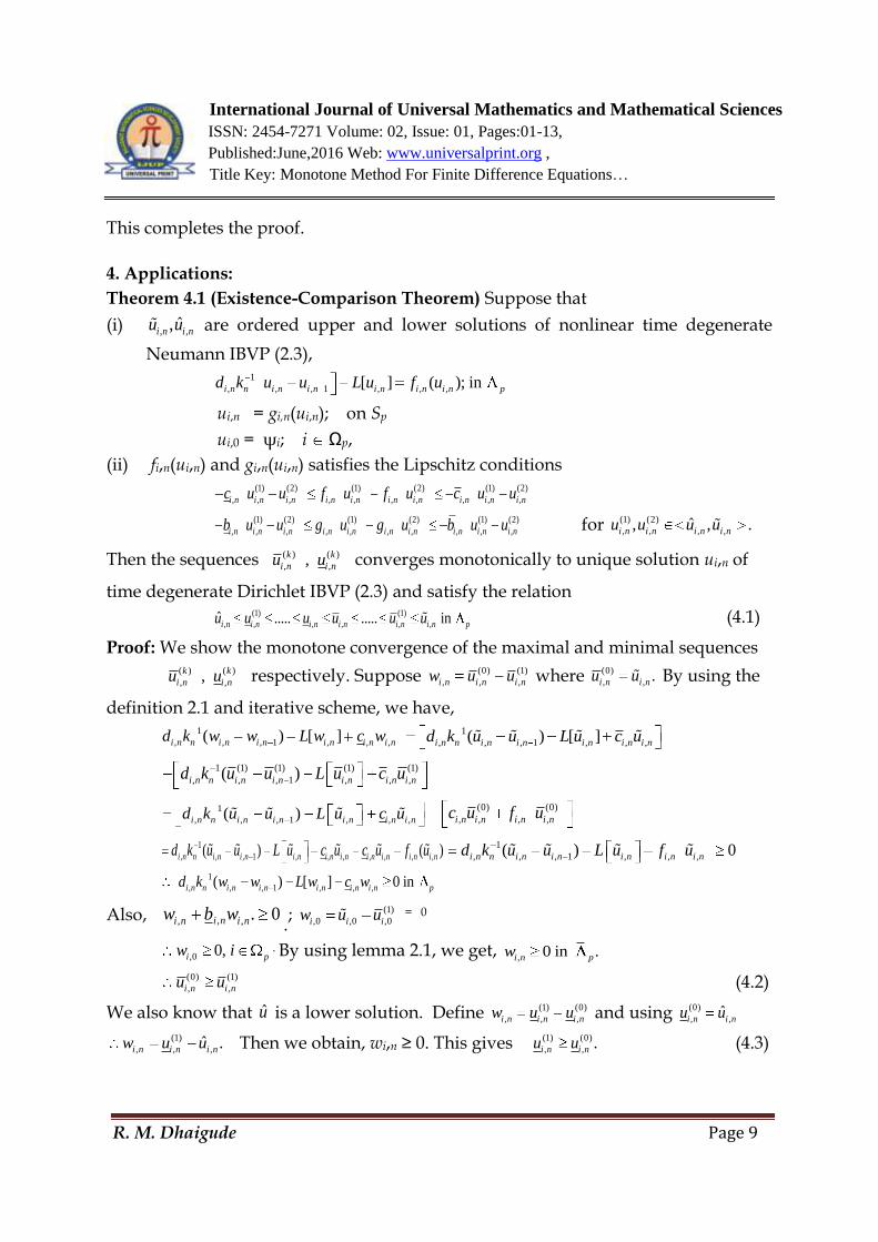
This completes the proof.

4. Applications:

Theorem 4.1 (Existence-Comparison Theorem) Suppose that

(i) , ,ˆ,i n i nu u are ordered upper and lower solutions of nonlinear time degenerate

Neumann IBVP (2.3),

1

, , , 1 , , ,[ ] ( ); ini n n i n i n i n i n i n pd k u u L u f u


ui,0 = ψi; i Ωp,

(ii) fi,n(ui,n) and gi,n(ui,n) satisfies the Lipschitz conditions (1) (2) (1) (2) (1) (2)


(1) (2) (1) (2) (1) (2)

, , , , , , , , , ,i n i n i n i n i n i n i n i n i n i nb u u g u g u b u u for (1) (2)

, , , ,ˆ, , .i n i n i n i nu u u u

Then the sequences ( ) ( )

, ,,k k

i n i nu u converges monotonically to unique solution ui,n of

time degenerate Dirichlet IBVP (2.3) and satisfy the relation (1) (1)

, , , , , ,ˆ ..... ..... ini n i n i n i n i n i n pu u u u u u (4.1)

Proof: We show the monotone convergence of the maximal and minimal sequences ( ) ( )

, ,,k k

i n i nu u respectively. Suppose (0) (1)

, , ,i n i n i nw u u where (0)

, , .i n i nu u By using the

definition 2.1 and iterative scheme, we have, 1

, , , 1 , , ,( ) [ ]i n n i n i n i n i n i nd k w w L w c w 1

, , , 1 , , ,( ) [ ]i n n i n i n i n i n i nd k u u L u c u

1 (1) (1) (1) (1)

, , , 1 , , ,( )i n n i n i n i n i n i nd k u u L u c u

1

, , , 1 , , ,( )i n n i n i n i n i n i nd k u u L u c u (0) (0)

, , , ,i n i n i n i nc u f u

1

, , , 1 , , , , , , ,( ) ( )i n n i n i n i n i n i n i n i n i n i nd k u u L u c u c u f u 1

, , , 1 , , ,( ) 0i n n i n i n i n i n i nd k u u L u f u

1

, , , 1 , , ,( ) [ ] 0 ini n n i n i n i n i n i n pd k w w L w c w

Also,

0.,,, ninini wbw.; (1)

,0 ,0 ,0i i iw u u = 0

,0 0,i pw i . By using lemma 2.1, we get, , 0 in .i n pw

(0) (1)

, ,i n i nu u (4.2)

We also know that u is a lower solution. Define (1) (0)

, , ,i n i n i nw u u and using (0)

, ,ˆ

i n i nu u

(1)

, , ,ˆ .i n i n i nw u u Then we obtain, wi,n ≥ 0. This gives (1) (0)

, , .i n i nu u (4.3)







Next suppose that (1) (1) (1)

, , , .i n i n i nw u u Then by using the given Lipschitz condition, and

by iterative scheme, we get,

1 (1) (1) (1) (1)

, , , 1 , , ,i n n i n i n i n i n i nd k w w L w c w(0) (0) (0) (0)

, , , , , , , ,i n i n i n i n i n i n i n i nc u f u c u f u

, , , , , , , ,

ˆ ˆi n i n i n i n i n i n i n i nc u f u c u f u

, , , ,ˆ 0 ini n i n i n i n pF u F u

1 (1) (1) (1) (1)

, , , 1 , , , 0i n n i n i n i n i n i nd k w w L w c w

Also wi,n(k) + bi,nwi,n(k) (0) (0)

, , , ,i n i n i n i nG u G u ≥0

(1)

,0 0, .i pw i

Thus by Lemma 2.1, we get

(1)

,0 0.iw (1) (1)

,0 ,0i iu u (4.4)

Thus by (4.2), (4.3) and (4.4), we get

(0) (1) (1) (0)

, , , , .i n i n i n i nu u u u

Assume by induction ( 1) ( ) ( ) ( 1)

, , , , ink k k k

i n i n i n i n pu u u u

Define a function ( ) ( ) ( 1)

, , ,

k k k

i n i n i nw u u

1 ( ) ( ) ( ) ( )

, , , 1 , , ,

k k k k


( 1) ( 1) ( ) ( )

, , , , , , , ,

k k k k


(By using definition 2.1 and iterative scheme)

( 1) ( )

, , , , 0k k


(By using Lipschtiz condition)

1 ( ) ( ) ( ) ( )

. , , 1 , , , 0; .k k k k


Also, wi,n(k) + bi,nwi,n(k ) ( 1) ( )

, , , , 0k k


( )

,0 0, .k

i pw i Then we obtain

( ) ( 1)

,0 , ,0. sok k k

i i n i nw u u (4.5)

Now define consider ( ) ( 1) ( )

, , ,

k k k

i n i n i nw u u ;

1 ( ) ( ) ( ) ( )

, , , 1 , , ,

k k k k


( ) ( ) ( 1) ( 1)

, , , , , , , ,

k k k k


(By using iterative scheme and Lipschitz condition), 1 ( ) ( ) ( ) ( )

, , , 1 , , , 0 ink k k k


Also wi,n(k) +bi,nwi,n(k) ( ) ( 1)

, , , , 0k k

i n i n i n i nG u G u ; ( )

,0 0,k

iw in Ωp







Then we obtain wi,n(k) ≥ 0. So ui,n(k+1) ≥ ui,n(k) (4.6)

1 ( ) ( ) ( ) ( )

, , , 1 , , ,

k k k k

i n n i n i n i n i n i nd k w w L w c w ( ) ( ) ( 1) ( 1)

, , , ,

k k k k

i n n i n n i n n i n nc u f u c u f u

(By definition 2.1 and using iterative scheme)

( ) ( )

, , , , 0k k


(By using Lipschtiz condition)

1 ( ) ( ) ( ) ( )

, , , 1 , , , 0; .k k k k


Also, wi,n(k) +bi,nwi,n(k) ( ) ( )

, , , , 0k k

i n i n i n i nG u G u ; ( )

,0 0, .k

i pw i

( )

, 0.k

i nw ; so ( 1) ( 1)

, ,

k k

i n i nu u (4.7)

Thus from (4.5), (4.6) and (4.7) we have, ( ) ( 1) ( 1) ( )

, , , , .k k k k

i n i n i n i nu u u u (4.8)

Thus monotone property (3.7) follows from principle of mathematical induction.

Now we conclude that the sequence ( )

,

k

i nu is a monotone nonincreasing and is

bounded from below hence it is convergent. Also the sequence ( )

,

k

i nu is monotone

nondecreasing and is bounded from above. Hence it is convergent. So, ( )

, ,lim k

i n i nk

u u

and ( )

, ,lim k

i n i nk

u u exists and called maximal and minimal solutions respectively of the

time degenerate parabolic Dirichlet initial boundary value problem (2.3) and they

satisfy (1) (2) (2) (1)

, , , , , , , ,ˆ ..... ...... .i n i n i n i n i n i n i n i nu u u u u u u u This completes the proof.

Theorem 4.2 [Uniqueness Theorem] Suppose that

(i) , ,ˆ,i n i nu u are ordered upper and lower solutions of time degenerate Dirichlet IBVP

(2.3) i.e. 1

, , , 1 , , ,( );( , )i n n i n i n i n i n i n pd k u u L u f u i n


ui,0 = ψi; i Ωp, with ,ˆ ,i nu u

(ii) The functions fi,n(ui,n) and gi,n(ui,n) satisfies the Lipschtiz condition (1) (2) (1) (2) (1) (2)


(1) (2) (1) (2) (1) (2)

, , , , , , , , , ,i n i n i n i n i n i n i n i n i n i nb u u g u g u b u u for (2) (1)

, , , ,ˆ .i n i n i n i nu u u u holds

1

, , , .i n n i n i nd k c b

Then the discrete problem (2.3) has a unique solution.

Proof : We know that , ,,i n i nu u are maximal and minimal solutions respectively of the

discrete time degenerate Dirichlet IBVP (2.3). To prove uniqueness we suppose that,

, , ,i n i n i nw u u 1

, , , 1 , , ,( ) ( )i n n i n i n i n i n i nd k w w L w f w , , , ,i n i n i n i nf u f u







, , ,i n i n i nc u u

, , .i n i nc w 1

, , , 1 , , ,( ) [ ] 0 ini n n i n i n i n i n i n pd k w w L w c w

1

, ,ˆ ˆ| | ( , ) ,i i i n i n i n i nx x w x t w x t b w

1ˆ ˆ| | ( , ) ,i i i n i nx x u x t u x t

1

, , , ,ˆ ˆ| | ( , ) ,i i i n i n i n i n i n i nx x u x t u x t b u b u

1

, ,ˆ ˆ| | ( , ) ,i i i n i n i n i nx x u x t u x t b u 1

, ,ˆ ˆ| | ( , ) ,i i i n i n i n i nx x u x t u x t b u

, , , , , , , ,i n i n i n i n i n i n i n i ng u b u g u b u

(by using iterative scheme),

, , , , 0; oni n i n i n i n pG u G u S

, , ,i n i n i nw u u = i – i = 0 in Sp

By using the positivity lemma we get , 0 ini n pw

, ,i n i nu u (4.9)

Also we can show that , ,i n i nu u (4.10)

Inequalities (4.9) and (4.10) implies that , ,i n i nu u in p. IBVP (2.3) has unique

solution.

Hence the result.

5 .Results: Extended the well known method of upper –lower solutions for

continuous parabolic problem to finite difference system of nonlinear time

degenerate parabolic Dirichlet initial boundary value problem.

6.Discussion: Researchers can be extend the well known method of upper –lower

solutions for continuous nonlinear parabolic problem to finite difference system of

nonlinear time degenerate parabolic Mixed initial boundary value problem .

7.Acknowledgement : I am thankful to Prof. D.B.

Dhaigude ,Department of Mathematics, Dr. Babasaheb Ambedkar Marathwada

University, Aurangabad for helpful discussions. We are also grateful to the referee

for his valuable suggestions.

References:

[1] Ames, W. F., Numerical Methods for Partial Differential Equations, (Third edition),

Academic Press, San Diego, 1992.

[2] Dhaigude, D. B., Sturmain Theorems for Time Degenerate Parabolic Inequalities. A.

St.Univ. “Al. I. Cza” Iasi Mathematics, (1990). 36: 35-39.







[3] Dhaigude, D. B. and Kasture, D. Y., Nonlinear Time Degenerate Parabolic Inequalities

and Application. J. Math. Anal. and Appl. (1993)., 175(2): 476-481.

[4] Dhaigude R. M., Monotone Method for Nonlinear Weakly Coupled Time

Degeneratre Parabolic System and Applications. Vidarbha Journal of Science (2012).,

7(1-2): 33-49.

[5] Forsythe, G. E. and Wasow, W. R., Finite Difference Methods for Partial Differentia

Equations, Weley, New York, 1964.

[6] Ippolite, P. M, Maximum Principles and Classical Solutions for Degenerate Parabolic

Equations, J. Math. Anal., 64 (1978), 530561

[7] Ladde, G. S., Lakshamikantham, V. and Vatsala, A.S., Monotone Iterative Techniques

for Nonlinear Digfferential Equations, Pitman, New York, 1985.

[8] Pao, C. V., Monotone iterative Method of Finite Difference System of Reaction

Diffusion Equations, Numer. Math., 46 (1985), 571-586.

[9] Pao, C. V., Nonlinear Parabolic and Elliptic Equation, Plenum Press, New York,

1992.

[10] Sattinger, D. H., Monotone Methods in Nonlinear Elliptic and Parabolic Boundary

Value Problems, Indiana Uni., Math. J., 21 (1972), 979-1000


Documents

Monotone Method for Finite Difference Equations Of ... · corresponds to the nonlinear reaction diffusion equations with linear ... first developed this method for nonlinear parabolic