Monotone Dynamical Systems and Some Models of Wolbachia …arima.inria.fr/020/pdf/vol.20.pp.145-176.pdf · Monotone Dynamical Systems and Some Models of Wolbachia in Aedes aegypti

Monotone Dynamical Systems and SomeModels of Wolbachia in Aedes aegypti

Populations

G. Sallet * — A. H. B Silva Moacyr **

* Département Institut Élie Cartan, UMR 7502Université de Lorraine, 57045 Metz Cedex 01, [email protected]

** Département Escola de Matemática Aplicada,Fundação Getulio Vargas,Praia de Botafogo 190, Rio de Janeiro, RJ Brésil, [email protected]

ABSTRACT. We present a model of infection by Wolbachia of an Aedes aegypti population. Thismodel is designed to take into account both the biology of this infection and any available data [30, 38].The objective is to use this model for predicting the sustainable introduction of this bacteria. Weprovide a complete mathematical analysis of the model proposed and give the basic reproduction ratioR0 for Wolbachia. We observe a bistability phenomenon. Two equilibria are asymptotically stable :an equilibrium where all the population is uninfected and an equilibrium where all the population isinfected. A third unstable equilibrium exists. We provide a lower bound for the basin of attraction ofthe desired infected equilibrium. We are in a backward bifurcation situation. The bistable situationoccurs with natural biological values for the parameters.

RÉSUMÉ. Nous présentons un modèle d’infection par Wolbachia d’une population d’ Aedes aegypti.Ce modèle est conçu pour à la fois prendre en compte la biologie de l’infection mais aussi les don-nées d’une expérimentation sur le terrain [30, 38]. L’objectif est d’utiliser ce modèle pour prévoirl’introduction permanente de cette bactérie dans la population de moustiques. Nous donnons uneanalyse mathématique complète du modèle proposé avec le calcul du taux de reproduction de baseR0 pour Wolbachia. On observe un phénomène de bistabilité. Deux équilibres sont asymptotique-ment stables : un équilibre où toute la population est non infectée et un équilibre où toute la popula-tion est infectée. Un troisième équilibre instable existe. Nous donnons un encadrement pour le bassind’attraction de l’équilibre souhaité. Il s’agit d’une situation de bifurcation rétrograde. Cette situationapparaît pour des valeurs biologiquement normales des paramètres.

KEYWORDS : Mathematical epidemiology, Wolbachia, Aedes, dynamical systems, stability, ODE.

MOTS-CLÉS : Épidémiogie mathématique, Wolbachia, Aedes, systèmes dynamiques,stabilité, EDO.

Special issue Nadir Sari and Guy Wallet, Editors

ARIMA Journal, vol. 20, pp. 145-176 (2015)

1. IntroductionWolbachia is a bacterium which infects arthropod species, including a high proportion ofinsects ( 60% of species). Its interactions with its hosts are often complex, and in somecases it is considered as an endosymbiont.The unique biology of Wolbachia has attracted a growing number of researchers interestedin questions ranging from the evolutionary implications of infection through to the use ofthis agent for pest and disease control : a public web site has been funded by the Na-tional Science Foundation of Australia (http://www.wolbachia.sols.uq.edu.au/about.cfm), and a research in pubmeb (http://www.ncbi.nlm.nih.gov/pubmed)typing wolbachia gives 1315 results.The bacterium was identified in 1924 by M. Hertig and S. B. Wolbach in Culex pipiens[26].While Wolbachia is commonly found in many mosquitoes it is absent from the speciesthat are considered to be of major importance for the transmission of human pathogens.The successful introduction of a life-shortening strain of Wolbachia into the dengue vectorAedes aegypti that decreases adult mean life has recently been reported [9, 20, 25, 42, 43,49, 67].Moreover it is estimated that the population of mosquitoes harboring Wolbachia is lessefficient to transmit dengue [30, 43, 62].Then it is considered that using Wolbachia can be a viable option for controlling theincidence of the dengue. This is peculiarly interesting since this approach is twofold : de-creasing the population of mosquitoes and decreasing the transmission. Other approacheslike Sterile Insect Techniques (SIT) [1, 15] act uniquely on population level. SIT consiststo release sterile males (either irradiated males or genetically modified) competing withwild ones. A drawback of this technique is the need to release continuously sterile males.On the contrary the successful establishment of Wolbachia infected population, in theory,does not require continuous release.In [18] a model is considered, to investigate the possibility for Wolbachia to invade ageneral population of hosts.The reference [9] develops discrete models to predict the severity of adult life-shorteningand in turn are used to estimate the impact on the transmission of dengue virus.Reference [12] proposes a continuous-discrete model to predict invasion and establish-ment in a population.A discrete model for establishment in a host population is studied in [16].The authors of [24, 25] use integral delay-equation model and two stage population struc-ture (juvenile/adult) to represent dynamics of spread in a host population.Leslie matrix discrete model is used in [49].Reference [57] considers discrete generations models.

Finally, in [52], reaction–diffusion and integro-difference equation models are used tomodel the spatio-temporal spread of Wolbachia in Drosophila simulans.

146 - ARIMA - Volume 20 - 2015

ARIMA Journal

Our model, unlike those mentioned above, takes into account the totality of the populationdynamics of mosquitoes, incorporating the three mosquito life-stages: egg, larva, andpupa. The adult life-stage is subdivided into three compartments: composed of youngfemale mosquitoes (aged 1–5 days, not mated, that do not yet lay eggs ), mature femaleand male mosquitoes. The reason is to take into account both the particular biology ofWolbachia and the possibility to incorporate biological data [38]. In many models somecompartments are lumped : E, L and P in an aquatic stage in [1], L and P in [66]. Whenhaving access to data we obtain numbers for Eggs, Larvae and Pupae. This is the reasonfor our choice. When compartments are lumped it is very difficult to interpret these datato obtain figures for the lumped compartments.

This paper is organized as follows : In section 2 we study dynamics of a population ofAedes aegypti, incorporating the Egg, Pupae, Larvae, immature and mature female. Assaid one rationale for the introduction of two stages in female is to model, in the sequel,the cytoplasmic incompatibility induced by Wolbachia infection. We analyze completelythis model. Section 3 is devoted to a complete model adapted for the characteristics ofWolbachia. A complete analysis is given and bistability and backward bifurcation areproven.

2. Population dynamics of wild Aedes mosquitoBefore presenting and analyzing the model of infection with Wolbachia we will needsome preliminaries and some results that will be used in the sequel.

2.1. The modelThe life cycle of a mosquito consists of two main stages: aquatic (egg, larva, pupa) andadult (with males and females). After emergence from pupa, a female mosquito needs tomate and get a blood meal before it starts hatching eggs. Then every 4 − −5 days it willtake a blood meal and lay 100−−150 eggs at different places (10−−15 per place). Forthe mathematical description, our model is inspired by the models considered in [14, 15].However, for biological applications, our model introduce the complete stages.However we will consider three aquatic stages, where the authors [15, 1] lump the threestages into a single aquatic stage. The rationale is to prepare for a subsequent model withinfection by Wolbachia. Furthermore, we split the adult stage into three sub-compartments,males, immature female and mature female which leads to the following compartments:

– Eggs E;– Larvae L;– Pupae P ;– Males M ;

Monotone Dynamical Systems and some Models of Wolbachia in Aedes aegypti Populations - 147

ARIMA journal

– Young immature females Y ; we consider a female to be in the Y compartment fromits emergence from pupa until her gonotrophic cycle has began, that is the time of matingand taking the first blood meal, which takes typically 3−−4 days.

– Mature females F , i.e., fertilized female.Parameters µE , µP , µY , µF and µM are respectively the death rate of eggs, larvae, pupae,immature female, mature females and males. The parameters ηE ,ηL, ηP , β are therespective rate of transfer to the next compartment. The parameter ν is the sex ratio. Inthis model, we use a density dependent death rate for the larvae stage since mosquitoeslarvae (anopheles and aedes) are density sensitive, which imply an additional densitymortality rate. We assume that eggs emergence is influenced by larvae density. Thedevelopment is regulated by a carrying capacity effect depending on the occupation of theavailable breeding sites. The parameter C is the carrying capacity related to the amountof available nutrients and space. Such an hypothesis is appropriate since mosquitoes onlyhave access to a finite number of potential breeding sites, and density-dependent larvalsurvival has been demonstrated at such sites. The parameter φ is the average amount ofeggs laid per fertilized female per unit of time.Mating is a complex process that is not fully understood. However, as discussed in [1]and references therein, the male mosquito can mate practically through all its life. Afemale mosquito needs one successful mating to breed lifelong [31]. It is admitted thatmosquitoes locate themselves in space and time to ensure they are available to mate.Therefore, it is reasonable to assume that in any case the immature female will mate andafterwards move to compartment F , or die. Thus a parameter like 1

β+µYcan represents

the mean time given by length of the first gonotrophic cycle of a female, i.e., the intervalfrom immediately after the mating to the first blood meal.We assume that all the parameters are constant. In reality, the mosquito population variesseasonally. Nevertheless, such a model should be a good approximation for a definiteseason.

E = φF − (µE + ηE)E

L = ηE E

(1− L

C

)+

− (µL + ηL)L

P = ηL L− (µP + ηP )P

Y = ν ηP P − (β + µY )Y

F = β Y − µF F

M = (1− ν) ηP P − µM M,

(1)

148 - ARIMA - Volume 20 - 2015

ARIMA Journal

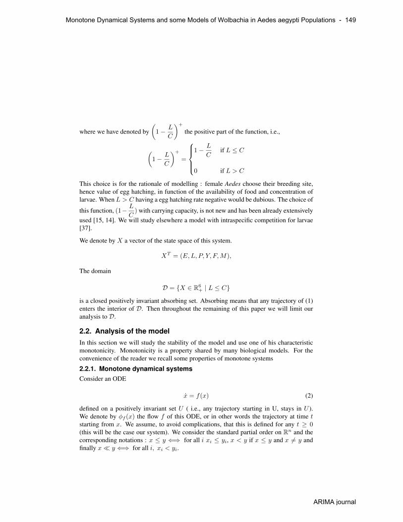
where we have denoted by(1− L

C

)+

the positive part of the function, i.e.,

(1− L

C

)+

=

1− L

Cif L ≤ C

0 if L > C

This choice is for the rationale of modelling : female Aedes choose their breeding site,hence value of egg hatching, in function of the availability of food and concentration oflarvae. WhenL > C having a egg hatching rate negative would be dubious. The choice of

this function, (1− L

C) with carrying capacity, is not new and has been already extensively

used [15, 14]. We will study elsewhere a model with intraspecific competition for larvae[37].

We denote by X a vector of the state space of this system.

XT = (E,L, P, Y, F,M),

The domain

D = {X ∈ R6+ | L ≤ C}

is a closed positively invariant absorbing set. Absorbing means that any trajectory of (1)enters the interior of D. Then throughout the remaining of this paper we will limit ouranalysis to D.

2.2. Analysis of the modelIn this section we will study the stability of the model and use one of his characteristicmonotonicity. Monotonicity is a property shared by many biological models. For theconvenience of the reader we recall some properties of monotone systems

2.2.1. Monotone dynamical systemsConsider an ODE

x = f(x) (2)

defined on a positively invariant set U ( i.e., any trajectory starting in U, stays in U ).We denote by φf (x) the flow f of this ODE, or in other words the trajectory at time tstarting from x. We assume, to avoid complications, that this is defined for any t ≥ 0(this will be the case our system). We consider the standard partial order on Rn and thecorresponding notations : x ≤ y ⇐⇒ for all i xi ≤ yi, x < y if x ≤ y and x 6= y andfinally x� y ⇐⇒ for all i, xi < yi.


ARIMA journal

System (2) is called monotone if x ≤ y implies φt(x) ≤ φt(y) [29, 28]. If f is C1 this

is equivalent to saying that the Jacobian of f , Jac(x) =(∂fi(x)

∂xj

)1≤i,j≤n

is a Metzler

matrix. A Metzler matrix is a matrix whose off-diagonal terms are nonnegative.

System (2) is called strongly monotone if x < y implies φt(x)� φt(y) for any t > 0.System (2) is strongly monotone if the Jacobian is irreducible. There is a simple algorithmto check if a Metzler matrix A is irreducible. The associated digraph G(A) of a n × nmatrix A, consists of n vertices 1, . . . j where an edge leads from j to i if and only ifaij 6= 0. A matrix A is irreducible iff its associated digraph is strongly connected, whichmeans that for any ordered pair (j, i) of vertices of G(A) , there exists a sequence oforiented edges (a path) which leads from i to j.We can use a different partial order associated to a cone. Let K = Rk+ × −(Rn−k+ ) and

the associated order defined by x ≤K y ⇐⇒ y − x ∈ K, x� y ⇐⇒ y − x ∈◦K.

The notion of monotony for this order ≤K will called of type K : monotone systems oftype K.

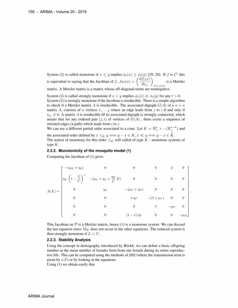
2.2.2. Monotonicity of the mosquito model (1)Computing the Jacobian of (1) gives

A(X) =

−(µE + ηE) 0 0 0 φ 0

ηE

(1− L

C

)+

−(µL + ηL +ηECE) 0 0 0 0

0 ηL −(µP + ηP ) 0 0 0

0 0 ν ηP −(β + µY ) 0 0

0 0 0 β −µF 0

0 0 (1− ν) ηP 0 0 −µM

.

This Jacobian on D is a Metzler matrix, hence (1) is a monotone system. We can discardthe last equation since MW does not occur in the other equations. The reduced system isthen strongly monotone if L < C.

2.2.3. Stability AnalysisUsing the concept in demography introduced by Böckh, we can define a basic offspringnumber as the mean number of females born from one female during its entire reproduc-tive life. This can be computed using the methods of [60] (where the transmission term isgiven by φF ) or by looking at the equations.Using (1) we obtain easily that

150 - ARIMA - Volume 20 - 2015

ARIMA Journal

R0,offsp =φ

µF

ηEµE + ηE

ηLµL + ηL

ν ηPµP + ηP

β

β + µY.

When R0,offsp ≤ 1 the only equilibrium is the origin. When R0,offsp > 1, a secondpositive equilibrium exists (E∗, L∗, P ∗, Y ∗, F ∗,M∗)T .We can express all the components as positive linear expressions of P ∗

L∗ =µp + ηpηL

P ∗, Y ∗ =ν ηPβ + µY

P ∗, (3)

F ∗ =β

β + µY

ν ηPµF

P ∗, M∗ =(1− ν) ηP

µMP ∗ (4)

E∗ =φ

µE + ηE

β

β + µY

ν ηPµF

P ∗. (5)

Finally, replacing in the equation L = 0, we get

P ∗ =R0 − 1

R0

C ηLµP + ηP

(6)

For a future use we will need positively compact invariant sets for (1) when R0,offsp > 1and when R0,offsp ≤ 1. In accordance with these notations the closed order interval [a, b]is

[ a, b ] = {x ∈ Rn | a ≤ x ≤ b}

We will also denote by X∗ = (E∗, L∗, P ∗, Y ∗, F ∗,M∗)T � 0.

Proposition 2.1When R0,offsp > 1, for any s and any θ such that 0 < s < 1 and 1 < θ the closed orderintervals

[ sX∗, θ X∗ ]

are positively invariant compact subsets of the positive orthant for system (1)

When R0,offsp ≤ 1, there exists Xk � 0 such that the order intervals [0, θ Xk] are posi-tively invariant compact subsets of the positive orthant for any θ ≥ 1.

ProofWe remark that the vector field associated to (1), A(X)X = f(X), is strictly sublinear.In other words this means that for any X � 0 and any 0 < λ < 1 we have

λ f(X) < f(λX).


ARIMA journal

From sublinearity we immediately obtain f(sX∗) > 0 and f(θ X∗) < 0. Using theproof of Proposition 2.1 we then obtain that [ sX∗, θ X∗ ] is positively invariant by themonotone system (1).When R0,offsp ≤ 1 we choose Lk = C, Pk = 2

ηLµP + ηP

Lk, Yk = 2ν ηPβ + µU

Pk,

Fk = 2β

µFYk, Mk = 2

(1− ν) ηPµM

Pk and Ek = 2φ

µE + ηEFk. If we define Xk =

(Ek, Lk, Pk, Yk, Fk,Mk)T we have f(Xk) � 0. By the same argument as before the

order interval [0, Xk] is a positively invariant absorbing set.This proves that all the trajectories are bounded.

�We can now give the main result of this section

Theorem 2.1IfR0,offsp < 1 the origin is globally asymptotically stable in the nonnegative orthant Rn+.In other words the mosquito population goes to extinction.If R0,offsp > 1 the positive equilibrium X∗ is globally asymptotically stable on the non-negative orthant minus the M -axis.

ProofSince M does not appear in the 5 first equations, to study the stability of system (1) it issufficient to consider the first 5 equations. In this case the system is strictly monotone andstrictly sub-linear. Moreover Proposition 2.1 shows that all the trajectories are bounded.We can apply Theorem 6.1 of [27], with a simple adaptation to strict sub linear systems.Hence all trajectories tend to the origin or else there is a unique equilibrium X∗ � 0 andall trajectories in R5

+ \ {0} tend to X∗.The origin is stable whenR0,offsp < 1. On the other hand X∗ is stable whenR0,offsp > 1and the origin is unstable. It is sufficient to consider the Jacobian at the equilibrium. Sincewe will have to do again these computations we refer to a subsequent section (3.4.1),where the stability of these matrices are proved. Actually the Jacobian computed at thepositive equilibrium is given by matrix A11 in (3.4.1). The stability of A11 is proven inthis section.When R0,offsp ≤ 1 we have only one equilibrium, which is the origin, in a set wherethe system is strongly monotone. Then using Theorem 10.3 of Hirsch [28] we obtain theglobal stability of the origin, in the open domain L < C. Since this domain is absorbingthis proves the global asymptotic stability.

�

For further reference we will denote by f(X,φ, µF , µK) the vector field on R6 associatedto (1). This is to stress some particular parameters which will be of importance later on.

152 - ARIMA - Volume 20 - 2015

ARIMA Journal

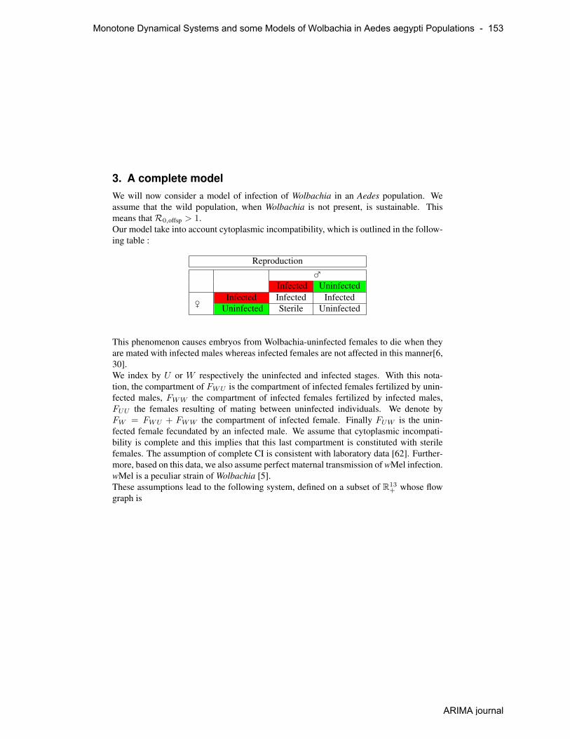
3. A complete modelWe will now consider a model of infection of Wolbachia in an Aedes population. Weassume that the wild population, when Wolbachia is not present, is sustainable. Thismeans thatR0,offsp > 1.Our model take into account cytoplasmic incompatibility, which is outlined in the follow-ing table :

Reproduction♂

Infected Uninfected

♀Infected Infected Infected

Uninfected Sterile Uninfected

This phenomenon causes embryos from Wolbachia-uninfected females to die when theyare mated with infected males whereas infected females are not affected in this manner[6,30].We index by U or W respectively the uninfected and infected stages. With this nota-tion, the compartment of FWU is the compartment of infected females fertilized by unin-fected males, FWW the compartment of infected females fertilized by infected males,FUU the females resulting of mating between uninfected individuals. We denote byFW = FWU + FWW the compartment of infected female. Finally FUW is the unin-fected female fecundated by an infected male. We assume that cytoplasmic incompati-bility is complete and this implies that this last compartment is constituted with sterilefemales. The assumption of complete CI is consistent with laboratory data [62]. Further-more, based on this data, we also assume perfect maternal transmission of wMel infection.wMel is a peculiar strain of Wolbachia [5].These assumptions lead to the following system, defined on a subset of R13

+ whose flowgraph is


ARIMA journal

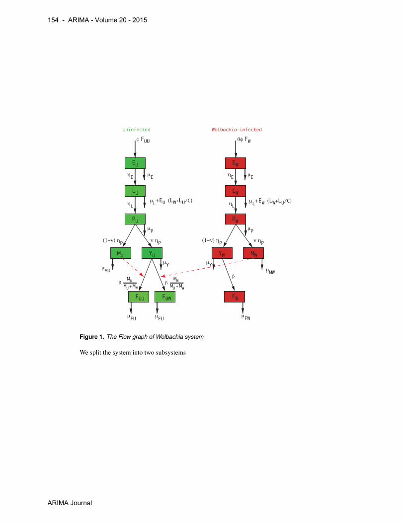
EU

LU

PU

YUMU

FUU

φ FUU

FUW FW

θφ FW

EW

LW

PW

YW MW

ηE

ηL

(1−ν) ηP ν ηP (1−ν) ηP ν ηP

μL+EW (LW+LU/C)μL+EU (LW+LU/C) ηL

μE μE

μPμP

μMU

μFU μFU μFW

μMW

μY μY

ηE

MUMWMU

β +

MWMWMU

β +

Uninfected Wolbachia-infected

β

Figure 1. The Flow graph of Wolbachia system

We split the system into two subsystems

154 - ARIMA - Volume 20 - 2015

ARIMA Journal

EU = φFUU − (µE + ηE) EU

LU = ηE EU

(1− (LU + LW )

C

)+

− [ηL + µL]LU

PU = ηL LU − (µP + ηP )PU

YU = ν ηP PU − (β + µY )YU

FUU = β YUMU

MU +MW− µFU FUU

MU = (1− ν) ηP PU − µMU MU

EW = θ φFW − (µE + ηE) EW

LW = ηE EW

(1− (LU + LW )

C

)+

− [ηL + µL]LW

PW = ηL LW − (µP + ηP )PW

YW = ν ηP PW − (β + µY )YW

FW = β YW − µFW FW

MW = (1− ν) ηP PW − µMW MW ,

(7)

and

FUW = β YUMW

MU +MW− µFU FUW . (8)

Since FUW (sterile female) does not appear in the other equations, due to cytoplasmicincompatibility, the asymptotic behavior of the complete system can be reduced to thebehavior of system (7), with (8) discarded. From now on, we will consider this reducedsystem. We will also restrict to the domain

D = {X | LU + LW ≤ C}. (9)

We have bounded cœfficients ( 0 ≤ MU

MU +MW≤ 1). Then in equations (7) we replace

MU

MU +MWby


ARIMA journal

h(MU ,MW ) =

MU

MU +MWif MU +MW > 0

0 if MU =MW = 0

System (7) is defined on R12+ \ {MU =MW = 0}.

We will denote byX = (XU , XW ) ∈ R6+×R6

+ the components of the state of the systemand we decompose accordingly the vector field in f = (fU , fV ). XU corresponds to theuninfected variables and XW corresponds to the Wolbachia-infected variables. System(7) can be written evidentlyXU

XW

=

AU (X) 0

0 AW (X)

XU

XW

With this choice the vector is globally Lipschitz and the nonnegative orthant R12

+ is posi-tively invariant.We will need, later on, to identify the invariant faces of R12

+ . It is clear that the only facespositively invariant are the four faces

{0}5 × R+ × R6 , R6+ × R+ × {0}5 , {0}6 × R6 , R6

+ × {0}6

of dimension 7, 7, 6, 6. We observe that the critical face {MU = MW = 0} is notpositively invariant.

We assume that Wolbachia has an impact on a stage when it is ascertained in litterature.However it would be straightforward to study a model for which Wolbachia has an impacton each stage. We incorporate a reduction of the mean life of the adult male and femalemosquito as quoted in the literature [9, 20, 25, 42, 43, 49, 67]. Then we denote by µFWand µMW respectively the death rate of female and male infected by Wolbachia. We alsointroduce a competition, for mating, between infected male and uninfected male.In this model EU , EW are the eggs compartments, respectively uninfected and infected.According to the literature, there is no apparent difference between infected and unin-fected eggs [39] . So we denote respectively by µE and ηE the common death rate andthe transition into the larvae compartments.Similarly LU and LW are the larval compartments. In this case we introduce an in-traspecific competition between larvae. Again, it seems that there is no known differencebetween infected and uninfected larvae [39]. Then we denote by µL and ηL the commondeath rate and transition rate to pupae compartments.We denote by PU and PW the uninfected and infected pupae compartments.We also introduce a factor θ ≤ 1 to consider an eventual decrease of the amount of laideggs by an infected female [30, 41, 42, 62, 67].

156 - ARIMA - Volume 20 - 2015

ARIMA Journal

We consider this model in the nonnegative orthant minus the set defined by {MU =MW = 0}. The nonnegative orthant is clearly positively invariant by this system. Wecan define the value of our system to be 0 at the origin, since the absence of populationis a singular point. Note that our vector field cannot be prolongated continuously onthe nonnegative orthant. However all the trajectories are defined on our domain. Thecompetition between males results in the loss of monotonicity.

3.1. Equilibria

3.1.1. Uninfected equilibrium : Wolbachia free equilibriumWhen there is no infection in the mosquito population, i.e., EW = LW = PW = YW =FW = FUW = MW = 0, model (7) reduces to model (1) of mosquito population. Thenin the sequel we will assume thatR0,offsp > 1. For this model the basic offspring numberis

R0,offsp,U =φ

µFU

ηEµE + ηE

ηLµL + ηL

ν ηPµP + ηP

β

β + µY.

In this case there is an equilibrium on the boundary of the nonnegative orthant whosecomponents are given by (3, 6), with the evident adaptation of notations corresponding tothe vector field f(X,φ, µFU , µMU ).This equilibrium corresponds to a population free of infection. We will call this equilib-rium the WFE ( Wolbachia free equilibrium). The WFE is expressed by (X∗U , 0) whereX∗U is given by (3, 6) with µF , µM replaced by µFU , µMU in the formulas.

3.1.2. Completely Wolbachia-Infected equilibriumIn a similar way if EU = LU = PU = YU = FUU = MU = 0 the system reduces toa system like (1) with different parameters. Actually this corresponds to the vector fieldf(θ φ, µFW , µMW ). Then we define a basic offspring number for the completely infectedpopulation

R0,offsp,W =θ φ

µFW

ηEµE + ηE

ηLµL + ηL

ν ηPµP + ηP

β

β + µY.

In this case there is an equilibrium on the boundary of the nonnegative orthant given by

P ∗W =C ηL

µP + ηP

(R0,offsp,W − 1)

R0,offsp,W(10)


ARIMA journal

L∗W =µP + ηPηL

P ∗W , Y ∗W =ν ηPβ + µY

P ∗W , (11)

M∗W =(1− ν) ηPµMW

P ∗W F ∗W =β

β + µY

ν ηPµFW

P ∗W , (12)

F ∗UW = 0, E∗W =θ φ

µE + ηE

β

β + µY

ν ηPµFW

P ∗W (13)

In the sequel, we will refer to this equilibrium as the “Completely Wolbachia-InfectedEquilibrium" (CWIE).Since we are addressing the issue of the sustainable establishment of Wolbachia we willassume in what follows thatR0,offsp,W > 1.

3.1.3. A coexistence equilibriumWe remark that

R0,offsp,W =θ µFUµFW

R0,offsp,U < R0,offsp,U .

This inequality implies that the infected population, as actually observed, would be smallerthat the uninfected population.

We denote by R0,W =θ µFUµFW

< 1. We will justify, later on that this notation: R0,W is

actually the basic reproduction ratio [60] for Wolbachia in the mosquito population.Then

R0,offsp,W = R0,W R0,offsp,U < R0,offsp,U . (14)

We assume that R0,offsp,W > 1. In this case a coexistence equilibrium exists in thepositive orthant. The components PU and PW are given by

PU,coex = CηL

ηP + µP

θ µFU µMU

µMW [µFW − θ µFU ] + θ µFU µMU

(R0,offsp,W − 1)

R0,offsp,W(15)

PW,coex = CηL

ηP + µP

µMW (µFW − θ µFU )µMW [µFW − θ µFU ] + θ µFU µMU

(R0,offsp,W − 1)

R0,offsp,W(16)

These two components are positive with our hypotheses. The remaining components canbe expressed in terms of these two as follows:

158 - ARIMA - Volume 20 - 2015

ARIMA Journal

LU,coex =µP + ηPηL

PU,coex, LW,coex =µP + ηPηL

PW,coex, (17)

YU,coex =ν ηPβ + µY

PU,coex , YW,coex =ν ηPβ + µY

PW,coex , (18)

MU,coex =(1− ν) ηPµMU

PU,coex, MW,coex =(1− ν) ηPµMW

PW,coex. (19)

(20)

FUU,coex =β ν ηPµMW

µFU (µMU PW,coex + µMW PU,coex) (β + µY )P 2U,coex, (21)

FW,coex =β ν ηP

µFW (β + µY )PW,coex, (22)

EU,coex =β ν φ ηP µMW

µFU (µMU PW,coex + µMW PU,coex) (β + µY ) (µE + ηE)P 2U,coex, (23)

EW,coex =β ν φ θ ηP

µFW (β + µY ) (µE + ηE)PW,coex. (24)

3.2. Monotonicity of the systemIn this section we will prove that our system is monotone for an order ≤K on the closedabsorbing positively invariant set D ( see 9) and strongly monotone on a dense subset ofD.We claim that system (7) is monotone relatively to the cone K = R6

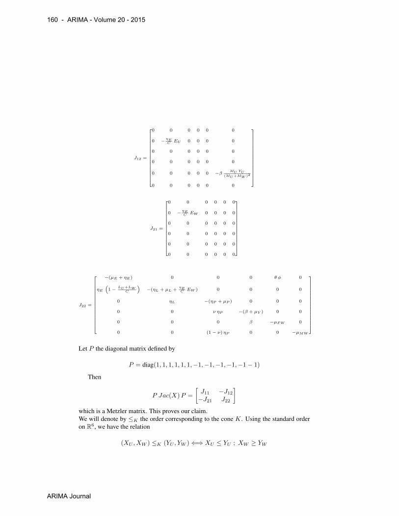
+ ×−(R6+) [53].

The Jacobian is given by the matrix block

J(X) =

[J11 J12J21 J22

]partitioned in 6× 6 blocks. The blocks are given by

J11 =

−(µE + ηE) 0 0 0 φ 0

ηE(1− LU+LW

C

)−(ηL + µL +

ηEC EU ) 0 0 0 0

0 ηL −(ηP + µP ) 0 0 0

0 0 ν ηP −(β + µY ) 0 0

0 0 0 β −µFU 0

0 0 (1− ν) ηP 0 0 −µMU


ARIMA journal

J12 =

0 0 0 0 0 0

0 − ηEC EU 0 0 0 0

0 0 0 0 0 0

0 0 0 0 0 0

0 0 0 0 0 −β MU YU(MU+MW )2

0 0 0 0 0 0

J21 =

0 0 0 0 0 0

0 − ηEC EW 0 0 0 0

0 0 0 0 0 0

0 0 0 0 0 0

0 0 0 0 0 0

0 0 0 0 0 0

J22 =

−(µE + ηE) 0 0 0 θ φ 0

ηE(1− LU+LW

C

)−(ηL + µL +

ηEC EW ) 0 0 0 0

0 ηL −(ηP + µP ) 0 0 0

0 0 ν ηP −(β + µY ) 0 0

0 0 0 β −µFW 0

0 0 (1− ν) ηP 0 0 −µMW

Let P the diagonal matrix defined by

P = diag(1, 1, 1, 1, 1, 1,−1,−1,−1,−1,−1− 1)

Then

P Jac(X)P =

[J11 −J12−J21 J22

]which is a Metzler matrix. This proves our claim.We will denote by ≤K the order corresponding to the cone K. Using the standard orderon R6, we have the relation

(XU , XW ) ≤K (YU , YW )⇐⇒ XU ≤ YU ; XW ≥ YW

160 - ARIMA - Volume 20 - 2015

ARIMA Journal

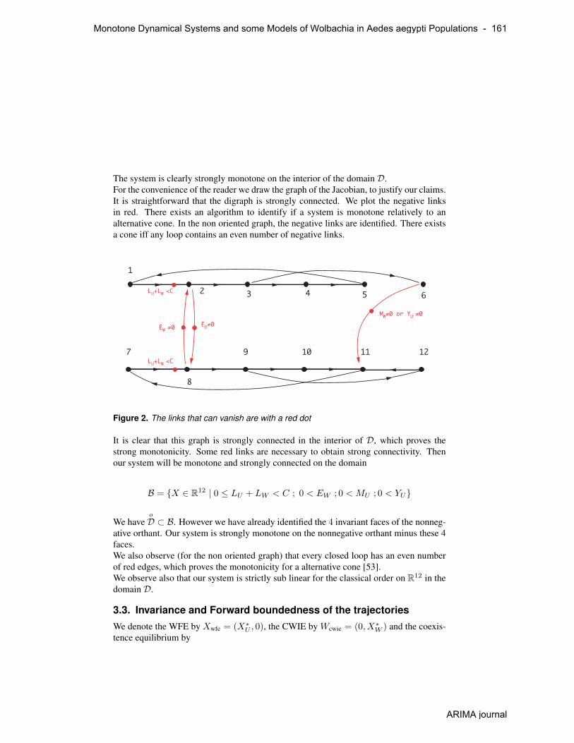
The system is clearly strongly monotone on the interior of the domain D.For the convenience of the reader we draw the graph of the Jacobian, to justify our claims.It is straightforward that the digraph is strongly connected. We plot the negative linksin red. There exists an algorithm to identify if a system is monotone relatively to analternative cone. In the non oriented graph, the negative links are identified. There existsa cone iff any loop contains an even number of negative links.

1

EU≠0 MW≠0 or YU ≠0

LU+LW <C

LU+LW <C

EW ≠0

2 3 4 5 6

7

8

9 10 11 12

Figure 2. The links that can vanish are with a red dot

It is clear that this graph is strongly connected in the interior of D, which proves thestrong monotonicity. Some red links are necessary to obtain strong connectivity. Thenour system will be monotone and strongly connected on the domain

B = {X ∈ R12 | 0 ≤ LU + LW < C ; 0 < EW ; 0 < MU ; 0 < YU}

We haveo

D ⊂ B. However we have already identified the 4 invariant faces of the nonneg-ative orthant. Our system is strongly monotone on the nonnegative orthant minus these 4faces.We also observe (for the non oriented graph) that every closed loop has an even numberof red edges, which proves the monotonicity for a alternative cone [53].We observe also that our system is strictly sub linear for the classical order on R12 in thedomain D.

3.3. Invariance and Forward boundedness of the trajectoriesWe denote the WFE by Xwfe = (X∗U , 0), the CWIE by Wcwie = (0, X∗W ) and the coexis-tence equilibrium by


ARIMA journal

Xcoex = (EU,coex, LU,coex, PU,coex, YU,coex, FUU,coex,MU,coex, . . .

EW,coex, EW,coex, LW,coex, PW,coex, FW,coex,MW,coex)T .

We will prove that

Xcoex <K Xcwie <K Xwfe.

Since Xcwie � 0, this is equivalent to X∗W > XW,coex and XU,coex < X∗U .Since f(Xcwie) = f(Xcoex) = f(Xcwie) = 0, this proves, by the argument already usedin the proof of Proposition 2.1, that for the order ≤K the order intervals

[Xcwie , Xcoex]K and [Xcoex , Xwfe]K

are positively compact invariant sets contained in D.We have also proved that for any ρ > 1, then f2(ρX∗W ) < 0 and f1(ρW ∗U ) < 0. Usingagain monotonicity, this proves that the order intervals

[ρ1Xcwie , Xcoex]K and [Xcwie , ρ2Xwfe]K

are positively invariant compact sets, as far as 1 ≤ ρ1 ≤C

L∗Wand 1 ≤ ρ2 ≤

C

L∗U(we

need monotonicity and then we are restricted to D). Using the relation for L∗W and L∗Uthis gives

ρ2 ≤ 1 +1

R0,offsp,W, ρ1 ≤ 1 +

1

R0,offsp,U.

For completeness we prove now our claims on comparisons of the 3 equilibria.We have

PU,coex + PX,coex = P ∗W .

Now, with relation (14) andR0,W < 1, we have

P ∗WP ∗U

=R0,W (R0,offsp,U − 1)

R0,W R0,offsp,U −R0,W )< 1

Using these two inequalities, it is now not difficult, using relations (10) to (21), to provethe desired inequalities for the equilibria. As a consequence the 3 equilibria are in thedomain D.We can find by an argument similar to Proposition 2.1 a vector Xk ∈ D such thatf(Xk) � 0. We begin to choose LU + Lk = C and we continue as in the Proposi-tion. Since f is monotone in D, the order set [0, Xk] is a positively invariant absorbingset. This proves that all the trajectories are bounded.

162 - ARIMA - Volume 20 - 2015

ARIMA Journal

3.4. Stability Analysis of the equilibriaIn this section we will prove the following Theorem

Theorem 3.1Trajectories of system ( 7) are forward bounded.

– IfR0,W R0,offsp,U = R0,offsp,W > 1,

three equilibria exist. A disease free equilibria (WFE), an equilibrium with the totalpopulation infected (CWIE) and a coexistence equilibrium in the positive orthant. TheWFE and CWIE are asymptotically stable, the coexistence equilibrium is unstable;

– IfR0,offsp,U > 1,

there exists an equilibrium without infection (WFE) which is asymptotically stable.

When R0,W <1

R0,offsp,Uonly the WFE exists and is globally asymptotically stable on

the nonnegative orthant minus the manifold MW = 0.

3.4.1. Stability of the Wolbachia Free EquilibriumTo study the stability of the infection free equilibrium WFE we compute the basic repro-duction ratio for the infection by Wolbachia. The variable corresponding to uninfectedcompartments

XU = (EU , LU , PU , YU , FUU ,MU ),

and the other variables for infected compartments

XW = (EW , LW , PW , YW , FW ,MW ).

We use the technique of [60] to compute the basic reproduction ratio for Wolbachia.

Since we are dealing with 12 equations, the verification of the hypothesis (A5) [60] isnot completely straightforward. Namely we have to prove (hypothesis A5) that, whenthe transmission is set to zero, then the Jacobian of the resulting system, computed atthe WFE, is a stable matrix (by stable we mean Hurwitz). Setting the transmission tozero amounts to set θ = 0. It is well known that the Jacobian computed at the WFE is adiagonal block upper triangular matrix :

Jac(WFE) =

[A11 A12

0 A22

].

In the present case A11 and A22 are 6× 6 matrices.


ARIMA journal

The matrix A22 when θ = 0 is equal to

A22 =

−(ηE + µE) 0 0 0 0 0ηE

R0,offsp,U−(µL + ηL) 0 0 0 0

0 ηL −(ηP + µP ) 0 0 00 0 νηP −(β + µY ) 0 00 0 0 β −µFW 00 0 (1− ν)ηP 0 0 −µMW

, (25)

and is clearly stable.

We now consider A11 :

A11 =

−(ηE + µE) 0 0 0 φ 0ηE

R0,offsp,U−µL + ηL

R0,offsp,U0 0 0 0

0 ηL −(ηP + µP ) 0 0 0

0 0 νηP −(β + µY ) 0 0

0 0 0 β −µFU 0

0 0 (1− ν) ηP 0 0 −µMU

.

The matrix A11 is a Metzler matrix. We can apply a lemma from [35], which we recallfor the convenience of the reader

Lemma 3.1Let M be a Metzler matrix, which is block decomposed :

M =

[A BC D

].

Where A and D are square matrices.Then M is Hurwitz if and only if A and D−CA−1B are Metzler stable.

We can now prove that A11 is Hurwitz. Since we have an evident eigenvalue −µMW inposition (6, 6); we can reduce the stability to the stability of the 5 × 5 principal upperblock.

V 5 =

−(ηE + µE) 0 0 0 φ

ηER0,offsp,U

− µL + ηLR0,offsp,U

0 0 0

0 ηL −(ηP + µP ) 0 00 0 νηP −(β + µY ) 00 0 0 β −µFU

.

If we define A = V 5(1 : 4, 1 : 4), the first upper 4× 4 block of V 5 and the other blocksaccordingly. Since the block A is lower triangular with a negative diagonal, we have the

164 - ARIMA - Volume 20 - 2015

ARIMA Journal

stability of this block. A computation of D − C A−1B, with this block decomposition,yields after some simplifications

D − C A−1B = −µFU(1− 1

R0,offsp,U

)< 0.

That proves that A11 is Hurwitz and finally that the hypothesis (A5) is satisfied.We can now compute the basic reproduction ratio for Wolbachia infection. We denote byF the Jacobian of all the transmission term in the infected compartments.

F =

0 0 0 0 θ φ 0

0 0 0 0 0 0

0 0 0 0 0 0

0 0 0 0 0 0

0 0 0 0 0 0

0 0 0 0 0 0

,

We denote by V the remaining part of the Jacobian A22 computed at the WFE.Using the results of [60], we know that the reproduction number for Wolbachia is givenbyR0,W = ρ(−F V 1). An immediate computation gives

−F V −1=

θ µFU

µFWR0,offsp,W

µE + ηE

ηE

θ φ β ν ηP

µFW (µP + ηP ) (β + µY )

θ φ β

µFW (β + µY )

θ φ

µFW0

0 0 0 0 0 00 0 0 0 0 00 0 0 0 0 00 0 0 0 0 00 0 0 0 0 0

.

Finally we obtain what we have already denoted asR0,W .

R0,W =θ µFU

µFW< 1.

This proves that the WFE is locally asymptotically stable.

3.4.2. Stability of the Completely Wolbachia-Infected EquilibriumIn this section, for the existence of the CWIE, we assume

1 < R0,offsp,W = R0,W R0,offsp,U < R0,offsp,U .

The Jacobian computed at the CWIE is a block diagonal lower triangular matrix


ARIMA journal

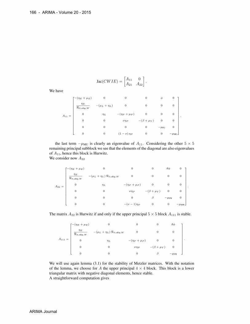
Jac(CWIE) =

[A11 0A21 A22

].

We have

A11 =

−(ηE + µE) 0 0 0 φ 0

ηE

R0,offsp,W−(µL + ηL) 0 0 0 0

0 ηL −(ηP + µP ) 0 0 0

0 0 νηP −(β + µY ) 0 0

0 0 0 0 −µFU 0

0 0 (1− ν) ηP 0 0 −µMU

.

the last term −µMU is clearly an eigenvalue of A11. Considering the other 5 × 5remaining principal subblock we see that the elements of the diagonal are also eigenvaluesof A11, hence this block is Hurwitz.We consider now A22

A22 =

−(ηE + µE) 0 0 0 θφ 0

ηE

R0,offsp,W−(µL + ηL)R0,offsp,W 0 0 0 0

0 ηL −(ηP + µP ) 0 0 0

0 0 νηP −(β + µY ) 0 0

0 0 0 β −µFW 0

0 0 −(ν − 1)ηP 0 0 −µMW

.

The matrix A22 is Hurwitz if and only if the upper principal 5× 5 block A111 is stable.

A111 =

−(ηE + µE) 0 0 0 θφ

ηE

R0,offsp,W−(µL + ηL)R0,offsp,W 0 0 0

0 ηL −(ηP + µP ) 0 0

0 0 νηP −(β + µY ) 0

0 0 0 β −µFW

.

We will use again lemma (3.1) for the stability of Metzler matrices. With the notationof the lemma, we choose for A the upper principal 4 × 4 block. This block is a lowertriangular matrix with negative diagonal elements, hence stable.A straightforward computation gives

166 - ARIMA - Volume 20 - 2015

ARIMA Journal

D − C A−1B = −µFW(1− 1

R0,offsp,W

)This proves finally the asymptotic stability of the CWIE.

3.4.3. Stability of the coexistence equilibriumWe will prove, in this section, that any trajectory in [Xcoex, Xwfe]K \{Xcoex} tends toXwfeand any trajectory in [Xcoex, Xcwie]K \ {Xcoex} tends to Xcwie.Then we will prove that the coexistence equilibrium is always unstable. Based on themonotonicity properties, this can be done without any computation. If we consider, forexample, the closed order interval [Xcoex, Xwfe]K , this interval is a compact positivelyinvariant and contain only two equilibria. This is almost a situation encountered in [28].

However we cannot apply Theorem 10.5 of Hirsch [28] which would give the desiredresult. To use this Theorem we need that our system is strongly monotone on our closedorder interval. This is not true since the face of this interval, contained in R6

+ × {0},is invariant. A key result for the proof of the Theorem of Hirsch is that the set of qua-siconvergent points, in a totally ordered arc for a strongly monotone system, is at mostcountable. A common difficulty in applying the Theorem of density, often overlooked inapplications, arises from the fact that irreducibility is an open condition. It commonlyoccurs that irreducibility holds only in the interior of the domain while some parts of theboundary are invariant sets. In this case, strong monotonicity (and even the strong orderpreserving property) may fail to hold on the boundary. This is exactly our case.For proving the result we need to tailor Hirsch’s Theorem to our situation. We will provea general result applicable to our situation.Then we consider on Rn+, strongly ordered by a coneK, a C1 monotone system x = f(x)with semiflow φ.We need to define what is a face of a closed order interval [p, q].

Definition 3.1The closed order interval [p, q] is a convex polytope, i.e, the finite intersection of half-spaces. A hyperplane H of Rn is supporting [p, q], at a point x ∈ [p, q], if one of the twoclosed halfspaces of H contains [p, q].A subset F of [p, q] is called a face of [p, q] if it is either ∅, [p, q] itself or the intersectionof [p, q] with a supporting hyperplane.

Theorem 3.2We consider a C1 monotone system x = f(x), whose flow φ preserves Rn+ for t ≥ 0.Let p, q be equilibria with p� q, with no other equilibria in [p, q].We assume that p is asymptotically stable for φ and that there exists a positively invariantface F of [p, q] containing p which is in the basin of p. We also assume that some otherfaces F1, F2, · · · , FK are positively invariant, and for any point x of each Fi, the omega-limit set satisfies ω(x) ∩ F 6= ∅.We assume that the system is strongly monotone on the complement


ARIMA journal

[p, q] \ (F ∪ F1 ∪ · · · ∪ Fk).

Then any trajectory of [p, q] \ {q} converges to p. Hence the equilibrium q is unstable.

ProofBy monotonicity [p, q] is a compact positively invariant set. Consequently any trajectoryin [p, q] is bounded.Consider the totally ordered arc in [p, q], J = {x = (1 − t) p + t q | 0 ≤ t ≤ 1}.If a point x ∈ I converges to p then by monotonicity [x, p] is in the basin of p. Sincep is asymptotically stable there exists x 6= p in J converging to p. Let a = sup{x ∈J | x converges to p}. Similarly let b = inf{x ∈ J | x converges to q}. The orderinterval [[a, b]] is composed of points converging neither to p, neither to q.The ordered interval [p, a]] is an open subset of [p, q], containing p in the basin of p.

We will show that a = b = q which will prove the Theorem.

Before this we show that any face Fi is in the basin of p. We know that for any x in Fi,ω(x) ∩ F 6= ∅. Since any point of F converges to p, by invariance of the omega limit set,we have p ∈ ω(x), which implies that the trajectory from x enters [p, a]] proving that xconverges to p.

To prove a = b, we proceed by contradiction assuming a � b. By definition of a and b,any point of [[a, b]] does not converge to an equilibrium. Moreover a cannot be in the basinof p. Otherwise, since p is asymptotically stable, the basin is open, which contradicts thedefinition of a. Let

W = φR+([a, b]] ∪ J).

Continuity of φ implies that W is a separable compact metric space positively invariantunder φ. Moreover W ∩ (F ∪F1 ∪ · · · ∪Fk) = ∅, otherwise this will implies that a pointof [[a, b]] converges to p, a contradiction. It follows that W is an ordered space, with astrongly monotone semiflow φ.The set W is a positively invariant compact ordered set with a strongly monotone semi-flow φ without equilibrium. By lemma 1.1 of [29], W has a maximal element z. Bymonotonicity φt(z) is an upper bound of W for any t ≥ 0. Hence z ≤ φt(z). If for at > 0 we have z < φt(z) by strong monotonicity, we can apply the convergence crtiterion(Theorem 1.4 [29]), z converges to an equilibrium. Otherwise z is an equilibrium. In anycase we have an equilibrium in W , which is a contradiction. This proves a = b.It remains to prove a = b = q. If b � q, [b, q] is a neighborhood of q, then q isasymptotically stable, hence the basin of q is open, which contradicts the definition of b.Hence a = b = q which ends the proof of the Theorem.

�

To prove our results we have only to consider the invariant faces where our system is notstrongly monotone. The face [Xcoex, Xcwie]K

⋂{0}×R6

+ is contained in the basin ofXcwie

168 - ARIMA - Volume 20 - 2015

ARIMA Journal

and is positively invariant. The positively invariant set, in which the system is not stronglymonotone, is exactly the two faces [Xcoex, Xcwie]K

⋂{0}×R6

+ and [Xwfe, Xcoex]K⋂

R6+×

{0} which are respectively in the basin of Xcwie and Xwfe. All the hypotheses of ourTheorem are satisfied.This proves that any trajectory in [Xcoex, Xcwie]K \ {Xcoex} tends Xcwie. This provesthat the coexistence equilibrium Xcoex is unstable. We have a similar result for the otherordered interval.

This result can be obtain directly : we compute the determinant of the Jacobian at thecoexistence equilibrium. We obtain after rearrangement and simplifications

det(Jac(Coex)) = (θ µFU − µFW )µFU µMU µMW (µE + ηE)2 (µL + ηL)

2

(µP + ηP )2 (β + µY )

2 (R0,offsp,W − 1) < 0 (26)

The negativity comes from (θ µFU − µFW ) < 0 and, since we are in dimension 12, thisproves the instability of the coexistence equilibrium.

3.4.4. More invariant setWe know that our system is strongly monotone on the interior of D for the order relativeto the cone ≤K .The coexistence equilibrium Xcoex = (XU,coex, XW,coex) is in the interior of D. Then thematrix P.Jac(Coex).P computed at this equilibrium is an irreducible unstable Metzlermatrix, where P is the diagonal matrix defined in section 3.2. By Perron-Frobenius thestability modulus s(Jac(Coex)) > 0 is an eigenvalue of the Jacobian and there exists apositive vector v � 0 such that

P.Jac(Coex) .P.v = s(Jac(Coex)) v

Hence P v = (vU ,−vW ) is an eigenvalue of the Jacobian. By Theorem 3.3 (p 62) andRemark 3.2 (p 63) of [53] we obtain that, for any ε > 0, following the order intervals

[(X∗U − ρ1 v1, 0) , Xcoex − ε(vU ,−vW )]K

and

[Xcoex + ε(vU ,−vW ) , (0, X∗W + ρ2 v2)]K

are positively compact invariant sets. Since each of these set contains an unique equi-librium, this proves that this unique equilibrium is globally asymptotically stable on theconsidered set.We have proven, using section 3.3, that [ρ1Xcwie , Xcoex]K is in the basin of attraction ofthe CWIE (0, X∗W ). An analogous result for the WFE.


ARIMA journal

W

Increasing order for W

Increasing order for U

X*W

XW,coex

ρ1 X*W

ρ2 X*UX*UXU,coex

Xcoex

R6

R6

Figure 3. Compact invariant sets for system (1), ρ1 and ρ2 defined in 3.3

We have obtained a lower bound for the basin of attraction of Xcwie. It is determined byXcoex and finally by the basic offspring numberR0,offsp,W .

3.5. What happens when R0,offsp,W ≤ 1 ?We can have upper bounds for the matrices AU (X) and AW (X). Using notations ofsection (3) we get

AU (X) ≤ A(X, θ, µFU , µMU ) AW (X) ≤ A(X, θ φ, µFW , µMW )

With the hypothesesR0,offsp,U > 1 andR0,offsp,W ≤ 1 we have already proved that

XU = A(X, θ, µFU , µMU ) XU

is globally asymptotically stable at a positive equilibrium X∗U ∈ R6+ and

XW = A(X, θ φ, µFW , µMW ) XW

has the origin for globally asymptotically stable equilibrium. Then by comparison The-orems of ODE for positive systems (all our matrices are Metzler) this proves that oursystem (7) converges to Xwfe.

170 - ARIMA - Volume 20 - 2015

ARIMA Journal

4. ConclusionThe phenomenon described above is now well known in epidemiological models, this isthe so-called backward bifurcation. See [2, 8, 59, 21] and references therein. Usually inepidemiological model when R0 < 1 the disease free equilibrium is stable and there areno other “infected" equilibria. At R0 = 1 an infected equilibrium bifurcates. In back-ward bifurcation there are infected equilibrium points in the domain R0 < 1. To quote[21] a general mechanism leading to backward bifurcations in epidemic models seemsunlikely. Backward bifurcations is known to occur in models with group structure andlarge differences between groups or models with interacting mechanisms (e.g. Vaccina-tion models or reinfection ). Our model does not enter in these categories. We can reduceour model, by lumping variables, to a very simple four dimensional system which alsoexhibits backward bifurcation. This result adds a new situation to the known ones.From the biological point of view, we have considered a complete model. We choosenot to lump some compartments and instead to distinguish those considered by biologists.This is for two reasons. Firstly it is easier for a biologist to understand our model andthen the data we have are related to biological compartments. Consideration of lumpedcompartments makes difficult and problematic data integration. Moreover this integrationneeds complex modeling assumptions. The objective of this paper was to check if, somedifferent modeling assumptions would modify previous results [37]. We observe that thismodel predicts that the successful establishment of Wolbachia in a population of Aedesaegyptii is possible. This has been observed in the field [30] for certain strain of Wol-bachia. Our model also predicts that the strain must not be too effective in the reduction

of the death rate. If R0,W =θ µFUµFW

is too small, then R0,offsp,W = R0,W R0,offsp,U will

be less than 1 preventing the successful establishment of Wolbachia. Unpublished dataseems to confirm that prediction.The authors thank the anonymous referees who helped, by their suggestions, to signifi-cantly improve the paper. The authors thank Claudia Codeço of Fiocruz for her help andP.A . Bliman, of INRIA and FGV, that caught their attention to Hirsch’s Theorem.

5. References

[1] R. ANGUELOV, Y. DUMONT, AND J. LUBUMA, “ Mathematical modeling of sterile insecttechnology for control of anopheles mosquito.”, Comput. Math. Appl., vol. 64, (2012), pp. 374–389.

[2] J. ARINO, C. C. MCCLUSKEY, AND P. VAN DEN DRIESSCHE, “Global results for an epidemicmodel with vaccination that exhibits backward bifurcation.”, SIAM J. Appl. Math., vol. 64(2003), pp. 260–276.

[3] R. BARRERA, M. AMADOR, AND G. G. CLARK, “Ecological factors influencing aedes ae-


ARIMA journal

gypti (diptera: Culicidae) productivity in artificial containers in salinas, puerto rico.”, J MedEntomol, vol. 43 (2006), pp. 484–492.

[3] N. H. BARTON AND M. TURELLI, “Spatial waves of advance with bistable dynamics: cyto-plasmic and genetic analogues of allee effects.”, Am Nat, vol. 178 (2011), pp. E48–75.

[4] G. BIAN, Y. XU, P. LU, Y. XIE, AND Z. XI, “The endosymbiotic bacterium wolbachia inducesresistance to dengue virus in aedes aegypti.”, PLoS Pathog, vol. 6 (2010), p. e1000833.

[5] M. S. C. BLAGROVE, C. ARIAS-GOETA, A.-B. FAILLOUX, AND S. P. SINKINS, “Wolbachiastrain wmel induces cytoplasmic incompatibility and blocks dengue transmission in aedes al-bopictus”, Proc Natl Acad Sci U S A, vol. 109 (2012), pp. 255–260.

[6] B. BOSSAN, A. KOEHNCKE, AND P. HAMMERSTEIN, “A new model and method for under-standing wolbachia-induced cytoplasmic incompatibility”, PLoS One, vol. 6 (2011), p. e19757.

[7] M. A. H. BRAKS, S. A. JULIANO, AND L. P. LOUNIBOS, “Superior reproductive success onhuman blood without sugar is not limited to highly anthropophilic mosquito species”, Med VetEntomol, vol. 20 (2006), pp. 53–59.

[8] F. BRAUER, “Backward bifurcations in simple vaccination models”, J. Math Anal Appl,vol. 298 (2004), pp. 418–431.

[9] J. S. BROWNSTEIN, E. HETT, AND S. L. O’NEILL, “The potential of virulent wolbachia tomodulate disease transmission by insects”, J Invertebr Pathol, vol. 84 (2003), pp. 24–29.

[10] M. H. T. CHAN AND P. S. KIM, “Modelling a wolbachia invasion using a slow-fast dispersalreaction-diffusion approach”, Bull Math Biol, vol. 75 (2013), pp. 1501–1523.

[11] N. CHITNIS, J. M. HYMAN, AND J. CUSHING, “Determining Important Parameters in theSpread of Malaria Through the Sensitivity Analysis of a Mathematical Model”, Bull. Math.Biol, vol. 70 (2008), pp. 1272–1296.

[12] P. R. CRAIN, J. W. MAINS, E. SUH, Y. HUANG, P. H. CROWLEY, AND S. L. DOBSON,“Wolbachia infections that reduce immature insect survival: Predicted impacts on populationreplacement”, BMC Evol Biol, vol. 11 (2011), p. 290.

[13] M. R. DAVID, R. LOURENCO-DE OLIVEIRA, AND R. M. D. FREITAS, “ Container produc-tivity, daily survival rates and dispersal of aedes aegypti mosquitoes in a high income dengueepidemic neighbourhood of rio de janeiro: presumed influence of differential urban structureon mosquito biology.”, Mem Inst Oswaldo Cruz, vol. 104 (2009), pp. 927–932.

[14] Y. DUMONT, F. CHIROLEU, AND C. DOMERG, “On a temporal model for the Chikungunyadisease: modeling, theory and numerics.”, Math Biosci, vol. 213 (2008), pp. 80–91.

[15] Y. DUMONT AND J. M. TCHUENCHE, “Mathematical studies on the sterile insect techniquefor the chikungunya disease and aedes albopictus”, J Math Biol, vol. 65 (2012), pp. 809–854.

[16] J. ENGELSTADTER, A. TELSCHOW, AND P. HAMMERSTEIN, “Infection dynamics of differ-ent wolbachia-types within one host population”, J Theor Biol, vol. 231 (2004), pp. 345–355.

[17] J. E. FADER AND S. A. JULIANO, “Oviposition habitat selection by container-dwellingmosquitoes: responses to cues of larval and detritus abundances in the field”, Ecol Entomol,vol. 39 (2014), pp. 245–252.

[18] J. Z. FARKAS AND P. HINOW, “Structured and unstructured continuous models for wolbachiainfections”, Bull Math Biol, vol. 72 (2010), pp. 2067–2088.

172 - ARIMA - Volume 20 - 2015

ARIMA Journal

[19] D. A. FOCKS, D. G. HAILE, E. DANIELS, AND G. A. MOUNT, “Dynamic life table modelfor aedes aegypti (diptera: Culicidae): simulation results and validation.”, J Med Entomol,vol. 30 (1993), pp. 1018–1028.

[20] F. D. FRENTIU, J. ROBINSON, P. R. YOUNG, E. A. MCGRAW, AND S. L. O’NEILL,“Wolbachia-mediated resistance to dengue virus infection and death at the cellular level.”, PLoSOne, vol. 5 (2010), p. e13398.

[21] K. HADELER AND P. VAN DEN DRIESSCHE, “Backward bifurcation in epidemic control.”,Math Biosci, vol. 146 (1997), pp. 15–35.

[22] P. A. HANCOCK AND H. C. J. GODFRAY, “Modelling the spread of wolbachia in spatiallyheterogeneous environments.”, J R Soc Interface, vol. 9 (2012), pp. 3045–3054.

[23] P. A. HANCOCK AND H. C. J. GODFRAY, “Modelling the spread of wolbachia in spatiallyheterogeneous environments.supplement online information.”, J R Soc Interface, vol. 9 (2012),pp. 3045–3054.

[24] P. A. HANCOCK, S. P. SINKINS, AND H. C. J. GODFRAY, “Population dynamic models ofthe spread of Wolbachia.”, Am Nat, vol. 177 (2011), pp. 323–333.

[25] P. A. HANCOCK, S. P. SINKINS, AND H. C. J. GODFRAY , “Strategies for introducingwolbachia to reduce transmission of mosquito-borne diseases.”, PLoS Negl Trop Dis, vol. 5(2011), p. e1024.

[26] M. HERTIG AND S. B. WOLBACH, “Studies on rickettsia-like micro-organisms in insects.”,J Med Res, vol. 44 (1924), pp. 329–374.

[27] M. HIRSCH, “The dynamical system approach to differential equations.”, Bull AMS, vol. 11(1984), pp. 1–64.

[28] M. W. HIRSCH, “Stability and convergence in strongly monotone dynamical systems.”, JReine Angew. Math, vol. 383 (1988), pp. 1–53.

[29] M. W. HIRSCH AND H. L. SMITH, “Monotone dynamical systems.”, in Handbook of differ-ential equations: ordinary differential equations. vol. Vol. II, (2005), pp. 239–357.

[30] HOFFMANN, A A AND MONTGOMERY, B L AND POPOVICI, J AND ITURBE-ORMAETXE,I AND JOHNSON, P H AND MUZZI, F AND GREENFIELD, M AND DURKAN, M AND LEONG,Y S AND DONG, Y AND COOK, H AND AXFORD, J AND CALLAHAN, A G AND KENNY, NAND OMODEI, C AND MCGRAW, E A AND RYAN, P A AND RITCHIE, S A AND TURELLI, MAND O’NEILL, S L, “Successful establishment of wolbachia in aedes populations to suppressdengue transmission.”, Nature, vol. 476 (2011), pp. 454–457.

[31] P. I. HOWELL AND B. G. J. KNOLS, “Male mating biology.”, Malar J, vol. 8 Suppl 2 (2009),p. S8.

[32] G. L. HUGHES, R. KOGA, P. XUE, T. FUKATSU, AND J. L. RASGON, “ Wolbachia infec-tions are virulent and inhibit the human malaria parasite plasmodium falciparum in anophelesgambiae.”, PLoS Pathog, vol. 7 (2011), p. e1002043.

[33] H. HUGHES AND N. F. BRITTON, “Modelling the use of wolbachia to control dengue fevertransmission.”, Bull Math Biol, vol. 75 (2013), pp. 796–818.

[34] I. ITURBE-ORMAETXE, T. WALKER, AND S. L. O’ NEILL, “Wolbachia and the biologicalcontrol of mosquito-borne disease.”, EMBO Rep, vol. 12 (2011), pp. 508–518.


ARIMA journal

[35] J. KAMGANG AND G. SALLET, “Computation of threshold conditions for epidemiologicalmodels and global stability of the disease free equilibrium(DFE).”, Math Biosci, vol. 213(2008), pp. 1–12.

[36] M. J. KEELING, F. M. JIGGINS, AND J. M. READ, “The invasion and coexistence of com-peting wolbachia strains.”, Heredity (Edinb), vol. 91 (2003), pp. 382–388.

[37] J. KOILLER, M. DA SILVA, M. SOUZA, C. CODEÇO, A. IGGIDR, AND G. SALLET, “Aedes,Wolbachia and Dengue.”, Research Report RR-8462, INRIA, vol. Jan. 2014.

[38] P. M. LUZ, C. T. CODECO, J. MEDLOCK, C. J. STRUCHINER, D. VALLE, AND A. P.GALVANI, “Impact of insecticide interventions on the abundance and resistance profile of aedesaegypti.”, Epidemiol Infect, vol. 137 (2009), pp. 1203–1215.

[39] A. MACIA, “Differences in performance of aedes aegypti larvae raised at different densities intires and ovitraps under field conditions in argentina.”, J Vector Ecol, vol. 31 (2006), pp. 371–377.

[40] R. MACIEL-DE FREITAS, C. T. CODECO, AND R. LOURENCO-DE OLIVEIRA, “ Daily sur-vival rates and dispersal of aedes aegypti females in rio de janeiro, brazil.”, Am J Trop MedHyg, vol. 76 (2007), pp. 659–665.

[41] C. J. MCMENIMAN, R. V. LANE, B. N. CASS, A. W. C. FONG, M. SIDHU, Y.-F. WANG,AND S. L. O’NEILL, “Stable introduction of a life-shortening wolbachia infection into themosquito aedes aegypti.”, Science, vol. 323 (2009), pp. 141–144.

[42] C. J. MCMENIMAN AND S. L. O’NEILL, “A virulent wolbachia infection decreases theviability of the dengue vector aedes aegypti during periods of embryonic quiescence.”, PLoSNegl Trop Dis, vol. 4 (2010), p. e748.

[43] L. A. MOREIRA, I. ITURBE-ORMAETXE, J. A. JEFFERY, G. LU, A. T. PYKE, L. M.HEDGES, B. C. ROCHA, S. HALL-MENDELIN, A. DAY, M. RIEGLER, L. E. HUGO, K. N.JOHNSON, B. H. KAY, E. A. MCGRAW, A. F. VAN DEN HURK, P. A. RYAN, AND S. L.O’NEILL, “A wolbachia symbiont in aedes aegypti limits infection with dengue, chikungunya,and plasmodium.”, Cell, vol. 139 (2009), pp. 1268–1278.

[44] M. Z. NDII, R. I. HICKSON, D. ALLINGHAM, AND G. N. MERCER, “Modelling the trans-mission dynamics of dengue in the presence of wolbachia.”, Math Biosci, vol. 262 (2015),pp. 157–166.

[45] M. OTERO, H. G. SOLARI, AND N. SCHWEIGMANN, “A stochastic population dynamicsmodel for aedes aegypti: formulation and application to a city with temperate climate.”, BullMath Biol, vol. 68 (2006), pp. 1945–1974.

[46] J. POPOVICI, L. A. MOREIRA, A. POINSIGNON, I. ITURBE-ORMAETXE, D. MC-NAUGHTON, AND S. L. O’NEILL, “Assessing key safety concerns of a wolbachia-based strat-egy to control dengue transmission by aedes mosquitoes.”, Mem Inst Oswaldo Cruz, vol. 105(2010), pp. 957–964.

[47] J. L. RASGON, “Using predictive models to optimize wolbachia-based strategies for vector-borne disease control.”, Adv Exp Med Biol, 627 (2008), pp. 114–125.

[48] J. L. RASGON AND T. W. SCOTT, “Impact of population age structure on wolbachiatransgene driver efficacy: ecologically complex factors and release of genetically modifiedmosquitoes.”, Insect Biochem Mol Biol, vol. 34 (2004), pp. 707–713.

174 - ARIMA - Volume 20 - 2015

ARIMA Journal

[49] J. L. RASGON, L. M. STYER, AND T. W. SCOTT, “Wolbachia-induced mortality as a mech-anism to modulate pathogen transmission by vector arthropods.”, J Med Entomol, vol. 40(2003), pp. 125–132.

[50] J. R. REY AND S. M. O’CONNELL, “Oviposition by aedes aegypti and aedes albopictus:influence of congeners and of oviposition site characteristics.”, J Vector Ecol, vol. 39 (2014),pp. 190–196.

[51] S. A. RITCHIE, B. L. MONTGOMERY, AND A. A. HOFFMANN, “Novel estimates of aedesaegypti (diptera: Culicidae) population size and adult survival based on wolbachia releases.”, JMed Entomol, vol. 50 (2013), pp. 624–631.

[52] P. SCHOFIELD, “Spatially explicit models of turelli-hoffmann wolbachia invasive wavefronts.”, J Theor Biol, vol. (215 (2002), pp. 121–131.

[53] H. L. SMITH, “Monotone dynamical systems: an introduction to the theory of competitiveand cooperative systems..”, Mathematical Surveys and Monographs., vol. 41, ( 1995).

[54] M. O. SOUZA, “Multiscale analysis for a vector-borne epidemic model.”, J Math Biol, vol. 68(2014), pp. 1269–1293.

[55] A. S. SPIELMAN, M. G. LEAHY, AND V. SKAFF, “Failure of effective insemination of youngfemale aedes aegypti mosquitoes.”, J Insect Physiol, vol. 15 (1969), pp. 1471–1479.

[56] L. M. STYER, S. L. MINNICK, A. K. SUN, AND T. W. SCOTT, “Mortality and reproductivedynamics of aedes aegypti (diptera: Culicidae) fed human blood.”, Vector Borne Zoonotic Dis,vol. 7 (2007), pp. 86–98.

[57] M. TURELLI, “Cytoplasmic incompatibility in populations with overlapping generations.”,Evolution, vol. 64 (2010), pp. 232–241.

[58] A. P. TURLEY, L. A. MOREIRA, S. L. O’NEILL, AND E. A. MCGRAW, “ Wolbachia infec-tion reduces blood-feeding success in the dengue fever mosquito, aedes aegypti.”, PLoS NeglTrop Dis, vol. 3 (2009), p. e516.

[59] P. VAN DEN DRIESSCHE AND J. WATMOUGH, “A simple SIS epidemic model with a back-ward bifurcation .”, J Math Biol, vol. 40 (2000), pp. 525–540.

[60] P. VAN DEN DRIESSCHE AND J. WATMOUGH, “reproduction numbers and sub-thresholdendemic equilibria for compartmental models of disease transmission.”, Math Biosci, vol. 180(2002), pp. 29–48.

[61] T. WALKER, P. H. JOHNSON, L. A. MOREIRA, I. ITURBE-ORMAETXE, F. D. FRENTIU,C. J. MCMENIMAN, Y. S. LEONG, Y. DONG, J. AXFORD, P. KRIESNER, A. L. LLOYD, S. A.RITCHIE, S. L. O’NEILL, AND A. A. HOFFMANN, “supplement to : The wmel wolbachiastrain blocks dengue and invades caged aedes aegypti populations.”, Nature, vol. 476 (2011).

[62] , “The wmel wolbachia strain blocks dengue and invades caged aedes aegypti popula-tions.”, Nature, vol. 476 (2011), pp. 450–453.

[63] R. K. WALSH, L. FACCHINELLI, J. M. RAMSEY, J. G. BOND, AND F. GOULD, “ Assessingthe impact of density dependence in field populations of aedes aegypti.”, J Vector Ecol, vol. 36(2011), pp. 300–307.

[64] C. R. WILLIAMS, P. H. JOHNSON, T. S. BALL, AND S. A. RITCHIE, “ Productivity andpopulation density estimates of the dengue vector mosquito aedes aegypti (stegomyia aegypti)


ARIMA journal

in australia.”, Med Vet Entomol, vol. 27 (2013), pp. 313–322.

[65] J. WONG, S. T. STODDARD, H. ASTETE, A. C. MORRISON, AND T. W. SCOTT, “ Oviposi-tion site selection by the dengue vector aedes aegypti and its implications for dengue control.”,PLoS Negl Trop Dis, vol. 5 (2011), p. e1015.

[66] H. M. YANG, M. D. L. D. G. MACORIS, K. C. GALVANI, AND M. T. M. ANDRIGHETTI,“Follow up estimation of aedes aegypti entomological parameters and mathematical mod-ellings.”, Biosystems, vol. 103 (2011), pp. 360–371.

[67] H. L. YEAP, P. MEE, T. WALKER, A. R. WEEKS, S. L. O’NEILL, P. JOHNSON, S. A.RITCHIE, K. M. RICHARDSON, C. DOIG, N. M. ENDERSBY, AND A. A. HOFFMANN, “Dy-namics of the "popcorn" wolbachia infection in outbred aedes aegypti informs prospects formosquito vector control.”, Genetics, vol. 187 (2011), pp. 583–595.

176 - ARIMA - Volume 20 - 2015

ARIMA Journal

Documents

Monotone Dynamical Systems and Some Models of Wolbachia …arima.inria.fr/020/pdf/vol.20.pp.145-176.pdf · Monotone Dynamical Systems and Some Models of Wolbachia in Aedes aegypti