Embed Size (px)
Citation preview

0 Fermi j+lational Accelerator Laboratory
FERMILAB-Pub-82/70-THY October, 1982
Monopolonium
CHRISTOPHER T. HILL Fermi National Accelerator Laboratory P.O. Box 500, Batavia, Illinois 60510
ABSTRACT
We examine the general properties of a monopole anti-monopole
boundstate. Lifetimes grow as the cube of the initial diameter and
range, for an SU(5) GUT monopole with mass:2xlO 16 GEV, from about 43
days for d:l fm. to 10" years for d:.l angstrom. We find about lo7
hadrons are produced by fraeplentation of gluons that are radiated by
classical Larmor radiation. In the final burst when the extended cores
overlap about 25 fundamental degrees of freedom of the full unified
gauge group are produced. We find that such objects would have been
produced in the early Universe at about the time of Helium synthesis and
their decay products and Larmor radiation may be observable.
4% Operatsd by Universities Research Association Inc. under contract with the United States Department of Energy

-2- FERMILAB-Pub-82/70-THY
I. Introduction
If the Universe is widely populated by magnetic monopoles it
becomes conceiveable that a monopole-antimonopole boundstate, i.e.
monopolonium, can be formed in the laboratory or may have been formed
naturally in the Universe at large. Such objects, though unstable, have
an interesting physical evolution in time, dependent upon their masses,
their initial classical radii and their core structure. For GUT
monopoles with masses of the order of 1016 GEV, the lifetimes of
monopolonium systems range from days, for an initial diameter of about a
fermi, up to many times the Universe' lifetime with diameter of about a
tenth of an angstrom or more. While behaving as a classical system as
long as r>rcore , they will radiate characteristic dipole radiation up
16 to high energies, Mmonopole~10 . "ihus a monopolonium system provides a
window on the physics of elementary processes up to the extremely high
energy scale characterized by it's mass and could, in principle, yield
information about all of the physics between current accelerator
energies and the grand unification scale! A single event would produce,
for example, about lo5 Z-bosons by classical dipole radiation alone.
In the final annihilation stages the extended cores of the monopole
and anti-monopole overlap and one expects to produce the elementary
gauge and Higg's bosons of the full unifying gauge group. his "last
gasp" of the monopolonium system is expected to be cataclysmic,
releasing 2x10 16 Gev (about a kilowatt-hour) in less than 10 -38 sec. we
expect here a spectacular explosion of hadrons with a total hadron
multiplicity from the entire process of order 107. In the present paper
we will discuss the expected yields and spectra of hadrons, photons,

-3- FERMILAB-Pub-82/70-THY
Z-,X-,Y-,and Higgs-bosons. mu.9, while not quite a "table-top"
experiment, the study of monopolonium decay processes, should nature
avail, would afford the best experimental view of grand unification that
one can presently imagine.
Moreover, in the early Universe we will argue that a sizeable and
potentially detectable abundance of ultra long-lived monopolonium may
have been formed. Remarkably, we find that this process would have
occured during the relatively late period of Helium synthesis and
depends only upon the assumption of the existence of an acceptable
abundance of ordinary heavy monopoles at that time. We do not address
the question of how the Universe may have arrived at that epoch with a
monopole abundance well below the closure density. Rather, we adopt the
view that we know the Universe did indeed pass through such a phase, and
if the monopole abundance is near the closure density today (if it is
not then the detection of monopoles in experiments will be virtually
impossible), then the existence of a substantial relic abundance of
monopolonium follows as a logical consequence. For GUT monopoles we
find that in a typical cosmologically averaged cubic light year
containing on average 10 32 monopoles, there will be today about 10'5
monopolonia and roughly 400 decays per year. In galaxies and clusters
these abundances and rate densities may be significantly larger. mere
may also exist mechanisms to significantly enhance the formation and we
view the above results as conservative lower limits. me objects of
larger diameter are spinning down producing radio frequency radiation
from which we may place lower bounds on the masses of GUT monopoles.
me cataclysmic decay events may produce visible cosmic ray and high
energy gamma ray events in large scale earth-bound or orbiting

-II- FERMILAB-Pub-82/70-THY
detectors. Indeed, monopolonium may be easier to find than monopoles
themselves. In this paper we will only discuss the formation of
monopolonium in some detail and will defer a systematic survey of
observational signatures and constraints to a forthcoming work (1) .
Much of our discussion will be sufficiently general that it applies
to any magnetic monopole, regardless of detailed structure, dependent
only upon masses, magnetic charges and cosmological density of
monopoles. Also, much of this discussion is presumed valid even for
monopoles that are dressed by a few nucleons. The further corrections
for monopoles dressed by heavy nuclei are no doubt estimable, but
insofar as relic monopolonium is concerned, we do not expect any such
phenomenon due to the rarity of heavy nuclei in the helium synthesis
phase of the early Universe. The remaining discussion will specialize
to the case of an N(5) GUT monopole, but may be readily taken over to
any other grand unified theory gauge group (2) . We shall neglect such
complications as the Rubakov-Callan effect (3) , which could conceivebly
enhance the monopolonium formation rates but which we otherwise do not
expect will significantly change things, eg. as in hadroproduction,
given the extremely short time scales that will be involved.

-5- FERMILAB-Pub-82/70-THY
II. Profile of Monopolonium
Assume for the sake of discussion that we have an SU(5) monopole
separated a distance r from an anti-monopole. For SU(5) we assume:
fix = 5x IO” GEV
&GUT = l/40 et M,
MPl e ,J’ Mx = 2 x 10“ Ge\l
me effective Rydberg for the monopolonium system at large
separation (r>>10-13 cm) is:
R = ?$,/2%= = M,~GeV)xZ43
Fl : M,/2. = ceA”ceA *es (2)
where gm is the magnetic charge and N the "monopole number":
5 = g ‘, PQ-: F$, j a.,,z 3.ZW~ges~ (3) r=
For SU(5) monopolonium the above Rydberg is valid only at distances
larger than a few fermi. As r becomes comparable to (hQCD) the SU(3)
color chromomagnetic field turns on. The chromomagnetic field
terminates at a distance scale of .2 fm<rClfm due to the confinement
effects of QCD, believed generally to be a shielding by color-magnetic
monopole like fluctuations in the ordinary QCD vacuum (4).

-6- FERMILAB-Pub-82/70-THY
For r = l/s, the U(1) group of electromagnetism decomposes into
the U(1) and diagonal generator of w(2) of the full Weinberg-Salam
electroweak model. For all scales less than a fermi the various Operant
coupling constants are evolving with energy by the usual logarithmic
renormalization effects. 'lbese renormalization effects lead to a net
evolution of the effective magnetic charge, gm (5) .
Remarkably, however, the evolution of gm is very small over the
full range of the desert, even thou@ these various heirarchical effects
are setting in and the individual coupling constants are evolving
considerably in this range. With ). a threshold parameter of O(l), the
magnetic coupling constant is:
E tl 1 GeJ $ = 1/4eL
IGd c E 5 hW,o 5 = 1/4e+. + l/34:
WI,- :.E’;AM, 1
3 _ = 1/44:+jP1~5;
where E is the characteristic energy scale = l/r.
These follow by considering the SU(5) monopole vector potential at
the scale E =;\MX where the three coupling constants, z,, g2, and g3 of
U(l)xSU(2)xSU(3) are all equal to gCUT (2, is the SU(5) normalized U(1)
coupling constant). We write:

T (3) -= 5 &u-r
where:
Ai&3 ( 0, 0, 1 ) -1 ,4
- A = J : J.i”%b\, -& -f, J-, i)
(4 ‘x = AiG%(o, O, 0, I ,-I)
p :
J- i diaq50, I, -2, 0, 0)
-7- FERMILAB-Pub-82/70-THY
mus, the resulting force between a monopole anti-monopole pair is:
IFI = $3, $= Ipqgj\ Cl)
Finally, we restore the Weinberg-Salam coupling constant normalization
to obtain eq.(4):
41 5 ~,I& = 3 jt I-- (f)
We thus see that at very short distances, gm z l/gGUT , which is
the correct t'Hooft-Polyakov result for an adjoint of Higgs bosons and
which corresponds to N=2, or an effective Schwinger charge in terms of
-8- FERMILAB-Pub-82/70-THY
the gauge group charge gGUT. But at very large distances we have the net
evolution of the coupling constants and the confinement effects of QCD
which shield the l/g3 terms and we have a pure electromagnetic monopole
with gm=1/2e. Hence, the SU(5) monopole has the Dirac value for the
magnetic charge. Numerically we see that gm2(r>>lfm) : 137/4 : 34.25,
while gm"(r = Mx-') : 40. ‘Ibe various heirarchy effects lead to only a
net 15% change in pm2 over the full range of the desert, and we shall
ignore these in our analysis of monopolonium energetics. However, we
will have to include these effects in our discussion below of gamma,
Z-boson, and hadron production via gluon jets.
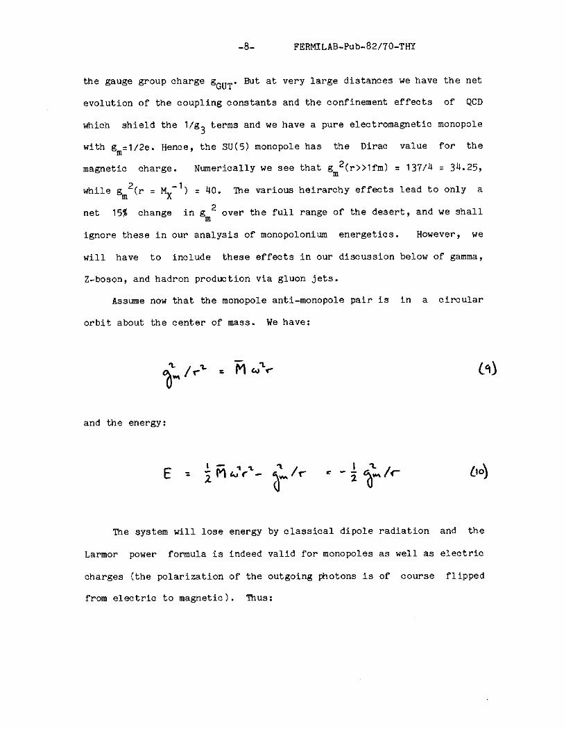
Assume now that the monopole anti-monopole pair is in a circular
orbit about the center of mass. We have:
and the energy:
E = i Fid:c’- y, 9
= - ; $t /c LIO)
The system will lose energy by classical dipole radiation and the
Larmor power formula is indeed valid for monopoles as well as electric
charges (the polarization of the outgoing photons is of course flipped
from electric to magnetic). Tnus:

-9- FERMILAB-Pub-82/70-THY
g = -2. (+) 5 (L..T;,‘/~ = - g ET(j-f-f-~i~~) 41)
by use of es.(g). Neglecting the slight renormalization evolution
effects of gm2, we thus have:
-I dE/ ~~ = 5 ( I&’ - $1
= t$ (tr - to)/' M;r') LIZ)
or:
T 2 r/\‘; rro3 g / ‘, a t13)
where in the last expression we've made use of eq.(lO).
Hence, the lifetime of the state is determined completely
classically and grows as the cube of the system's initial diameter. In
Table(I) we give numerical values of the lifetime vs. classical
diameter, en=-gy, principal quantum number and v/c. Remarkably, a
system of a GUT monopole with ~10~'~ cm lives about 43 days while with
I-= l/IO Angstrom, about a tenth the size of a hydrogen atom, we obtain
IO” years! This latter result raises the spectre of relic monopolonium
produced in the very early Universe surviving up to the present and
decaying today. We return to this question in Section IV.

-lO- FERMILAB-Pub-82/70-THY
The classical decay of the system may be viewed quantum
mechanically as a cascade of jumps throu@ sequentially decreasing
principal quantum numbers. lhe energy is given by the virial theorem
and by the Bohr formula (6):
E= -; Jra = /r = - R/n%
WC? see in Table(I) that the principal quantum number of the
instantaneous orbit is O(40) as v/c-->I. Simultaneously the orbital
diameter approaches the core size of a the GUT monopole, r-->l/MX.
me instantaneous transition energy is given by:
E’ ‘,
'me classical Larmor power formula for the rate of producing photons of
energy, E', is expected to be quite accurate for n>l (we note in passing
that even the 2P-->lS hydrogen transition rate can be computed to 30%
accuracy classically (6) 1. me instantaneous value of n gives, of course,
the total number of quanta radiated with energy E>E'. For all of our
subsequent discussion, excluding the core burst, n is safely >40.
From eq.(l5) we have the differential number of photons radiated in
a window of energy E' to E'+dE':

-ll- FERMILAB-Pub-82/70-THY
An z? =
q&t p?
me system decays by emitting photons until E' becomes greater than the
pion threshold, when r-->lO -18 cm and the lifetime remaining is 10 -9
set, and n=4.2xlO 6 . Here the system is beginning to radiate both photons
and gluons by classical dipole transitions with relative probabilities
that may be read off from eq.(4):
p$ : pg\“” - 1/4f2 : (1/3%;)F(E’) 117)
Here, f(E') is an unknown hadronic threshold function which is zero for
E'c m,, and should approach unity rapidly as El-->1 GEV. A few low
energy hadrons are expected in this phase of the decay, but rapidly as
E' exceeds 10 GEV, the gluon production leads to the formation of jets
of hadrons. Since this behavior sets in when the remaining lifetime is
only 10 -12 set while the principal quantum number is of order lo6 we do
not expect that the jets would be resolvable as "spikes" of hadrons
until very high energies (see Section III.), but rather as a continuous
distribution in space which may follow the l-cos2( 0 ) spatial
distribution of the Larmor radiated gluons reasonably well. Below we
consider both the multiplicity and energy distribution of the hadrons in
the resulting jets.
Furthermore, as the system passes throu& the principal quantum
number, n : 4~10~ , the Z" threshold opens up as the U(1) of
electromagnetism decomposes into the U(1) and diagonal generator of the

-12- FERMILAB-Pub-82/70-THY
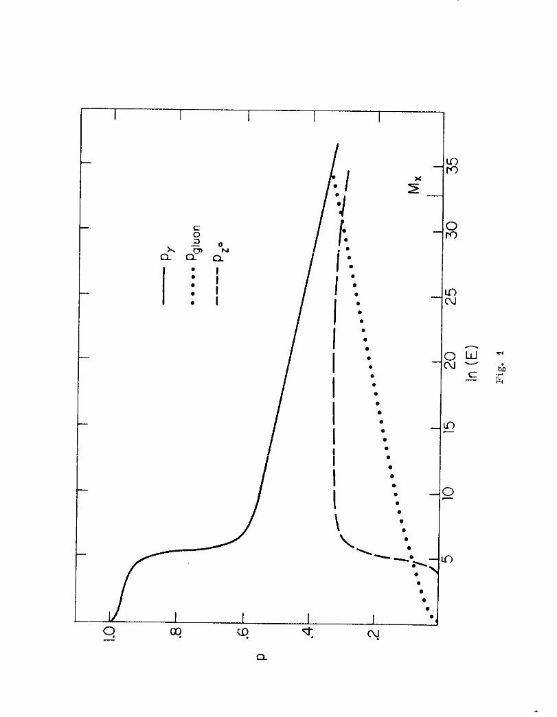
SU(2) of the electroweak theory. Now the relative probabilities of
photons, Z-bosons, and gluons become:
px’ pLO:pjdon ‘v &+ 2g!g:
( Si2& T!J c- .
-g+ $ - 1 +fj-i Cd
where 3 g,, g2, g3 are9 of course,energy dependent. In Fig.(l) the
normalized probabilities to produce the three different quanta are
plotted vs. In(E) from 1 GEV up to the GUT scale. Here we've built in
threshold factors of the form:
and we've taken p=2 though the overall physics is insensitive to the
choice of p>l. We further choose Ethr=l for gluons and MZ"=95 GEV for
the Z-boson. Above all thresholds we note that the three normalized
probabilities are simply expressed in terms of the running coupling
constants:
P ( I $5 I
y = $:$ $+ 4; p

-13- FERMILAB-Pub-82/70-THY
p,. =(2/y + $~~.~
p$“o, = (4/3 5) D’
D = ‘/c$ + ‘/$ + “/3$
From eq.(16) we therefore have the number of quanta of species i
produced in an energy window E to E+dE:
&; 2’3 d” -= AcE
-j- y;(E) ii4”
Quantitatively we note that the direct rate of production of gamma's
exceeds that of Z-bosons which in turn greatly exceeds that of gluons
until very high energies (provided we are above the Ztthreshold). We
find by a numerical integration that from a scale of 1 GEV up to MX that
the total number of direct photons is 4~10~ while there are 2.3~10~
Z-bosons and 1.3~10~ gluons produced. In Fig(2) we plot the three
multiplicity distributions
me framentation of gluons into high multiplicity jets of hadrons
and secondary decay products, including photons from $ decays,
substantialy modifies the spectrum. Most of the relatively soft photons
will be secondaries in this range. We first estimate the total yield of
hadrons. In QCD the multiplicity of charged hadrons prodwed in a gluon
jet of energy E is expected to be given in leading log QCD (7):
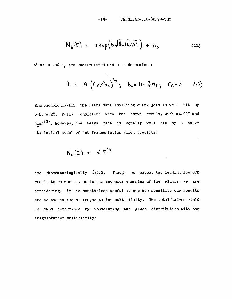
-14- FERMILAB-Pub-82/70-THY
N,(E) = aexl(bJm) + n,,
where a and no are uncalculated and b is determined:
b = 4 (Cn/boPj b,= II- ;fi+; c~=3 03)
Fhenomenologically, the Petra data including quark jets is well fit by
b-2.7+.28, fully consistent with the above result, with a=.027 and
n0:2(8). However, the Petra data is equally well fit by a naive
statistical model of jet fragmentation which predicts:
N,(E) = d E”’
and phenomenologically 2=2.2. lhou& we expect the leading log QCD
result to be correct up to the enormous energies of the gluons we are
considering, it is nonetheless useful to see how sensitive our results
are to the choice of fragmentation multiplicity. lhe total hadron yield
is thus determined by convoluting the gluon distribution with the
fragmentation multiplicity:

-15- FERMILAB-Pub-82/70-THY
N, = I”1 (5
WE\ 3 p+o. (E) i-+3 AE 0s) E,- IO
We find a total yield of -lo7 hadrons for the leading log QCD
fragmentation and 7x10* for the E (l/2) fragmentation distribution (the
naive parton model predicts a In(E) multiplicity in a jet which is
already inconsistent with the low energy data and we thus exclude it.)
We may further estimate the spectrum of hadrons and secondary
photons, though here we are on somewhat thinner ice. me exact x-
distribution for fragmentation of a gluon jet is not known, and only a
few properties, such as the total multiplicity and more recent
observations of a peak at very low x have been determined. (7) Indeed, it
is not clear how much can be determined theoretically. For our purposes
the important features are to realize the correct multiplicity, assure
that the first moment of the distribution be normalized properly to
unity, and try to guess the correct large-x behavior, which we take to
be (1~)~. We will build the multiplicity into the low-x behavior of the
distribution. For the leading log QCD multiplicity formula we find that
the following distribution works reasonably well:
AN\. - = AX
N&l .x, [bs) -$$- (1-b)
where N(b) is determined by the condition that the first moment of the
distribution is normalized to unity (energy conservation). We obtain:
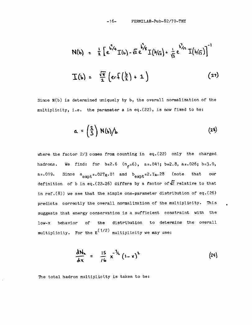
-16- FERMILAB-Pub-82/70-THY
N(b) = ; [t-?4~(+Jie%~(b,c)+ $-%(b,fi)j’
I(b) = $ [4(p) + 1)
Since N(b) is determined uniquely by b, the overall normalization of the
multiplicity, i.e. the parameter a in eq.(22), is now fixed to be:
a = (:j w/b
where the factor 213 comes from counting in eq.(22) only the charged
hadrons. We find: for bz2.6 (nf:6), az.041; bz2.8, a-.026; bz3.0,
az.019. Since a expt~.027t.01 and b expt=2.7i.28 (note that our
definition of b in eq.(22-26) differs by a factor of& relative to that
in ref.(8)) we see that the simple one-parameter distribution of eq.(26)
predicts correctly the overall normalization of the multiplicity. This .
suggests that energy conservation is a sufficient constraint with the
low-x behavior of the distribution to determine the overall
multiplicity. For the E(1'2) multiplicity we may use:
Ati, -= AX
fb x -x (\-xl=
me total hadron multiplicity is taken to be:

-l7- FERMILAB-Pub-82/70-THY
which may be seen to yield the correct multiplicity growth with energy
when the infra-red cutoff, E , is taken to be:
f = r / Ejet r - d.Gd
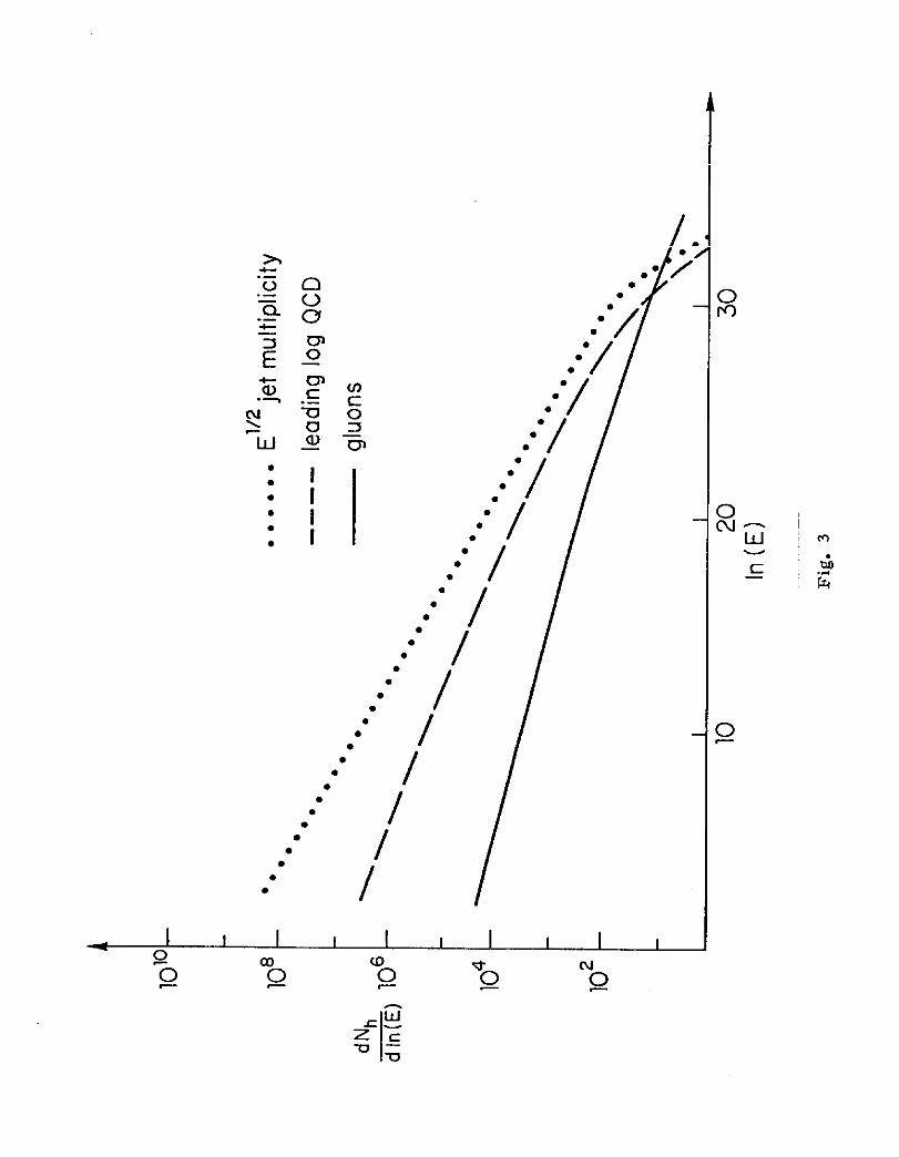
me fragmentation distributions are converted into hadron energy
distributions and are convoluted with the gluon distribution from
eq.(21) to obtain the hadron energy spectrum, e.g. for the leading log
QCD distribution we obtain:
AN\, @? - = ,N(h) AW)
(I- AF;’ (39
E
We choose as the upper limit of this convolution the energy scale
corresponding to the point at which the cores of the monopoles are
overlapping. To this we will add below the contributions from the final
burst, but this will be found to be a small correction to the total
hadron spectrum. me hadrons we count do not include the neutrals that
end up as photons. Here we may again appeal to the Petra data in which
the naive expectation that about 30% of the total distribution oonverts
quickly to photons is born out. me results are plotted in Fig.{31
along with the gluon distribution, for both multiplicity growth

-18- FERMILAB-Pub-82/70-THY
assumptions. me photon distribution can be taken to be 30% of the
hadron spectrum. We see that the hadron spectrum is somewhat softer
than the gluon distribution, as expected, though it tails up to
E~5xlO'~. me hadrons ultimately end up as gammas, electrons, nucleons
and neutrinos, as well as & and muons, at a distance range applicable
to astrophysical detection. We note that at accelerator energies the
baryon yield in jets is anomalously higher than one would have expected
from naive hadronization ideas and constitutes about 10% of the
spectrum. This may continue up to the enrgies under consideration here
and, if so, we may have a novel mechanism for producing cosmic rays by
the decays of relic monopolonium (see Section IV.).
__ me Burst III. --
Reference to Table(I) shows that at a principal quantum number of
n=40 the classical diameter of the monopolonium system has shrunk to
r=10m2' cm : 11 Mx and the cores of the monopoles themselves are now
overlapping. Simultaneously v/c-->1 and our classical approximations
are invalid. At this stage we still have about 75% of the system's
total energy to liberate. Here we expect to produce a burst of
particles of all types contained in the bare unified gauge theory.
A simple approximation to the physics of the burst is to assume
that the system's total energy is uniformly distributed throughout a
local region of diameter 2/MX. Particle multiplicities are then
determined by a universal amplitude and by phase space alone. Similar
statistical models are successful in hadroproduction at high energy (9).
Such a model neglects coherent or thermalization phenomena. Should the
system go into a "fireball" phase at this point we expect a much higher

-1g- FERMILAB-Pub-82/70-THY
yield of lower energy particles and a lower yield of the unified group
gauge bosons, X- and Y-, etc.
me universal amplitude, A, will be seen to have dimensions of area
and is expected to be related to the volume of the system:
A* &I?~ .w 2.6 RT - 5 Y
In what follows we closely parallel the analysis of ref.(lO).
me partial width to produce n identical bosons is:
r” = t; . i ! i [$& (27J4 Sk - ff;) i I
(53)
(34)
We neglect here an overall common normalization which we will not need
to know. It is expedient to consider the quantity:
caEojlM = $ i t2$,, caEi \ I
dt, ;ila-gfll.’ i F 3
= ; p 2Q.x [\i& e+* -a’3 (3d
where Q = (Eo,O,O,O) and use has been made of energy conservation,
Eo=& and the energy-momentum delta function has been replaced by it's
integral representation. In the end the parameter, a, will cancel. We
may perform the integral in the bracket for massless particles, po=Eo:
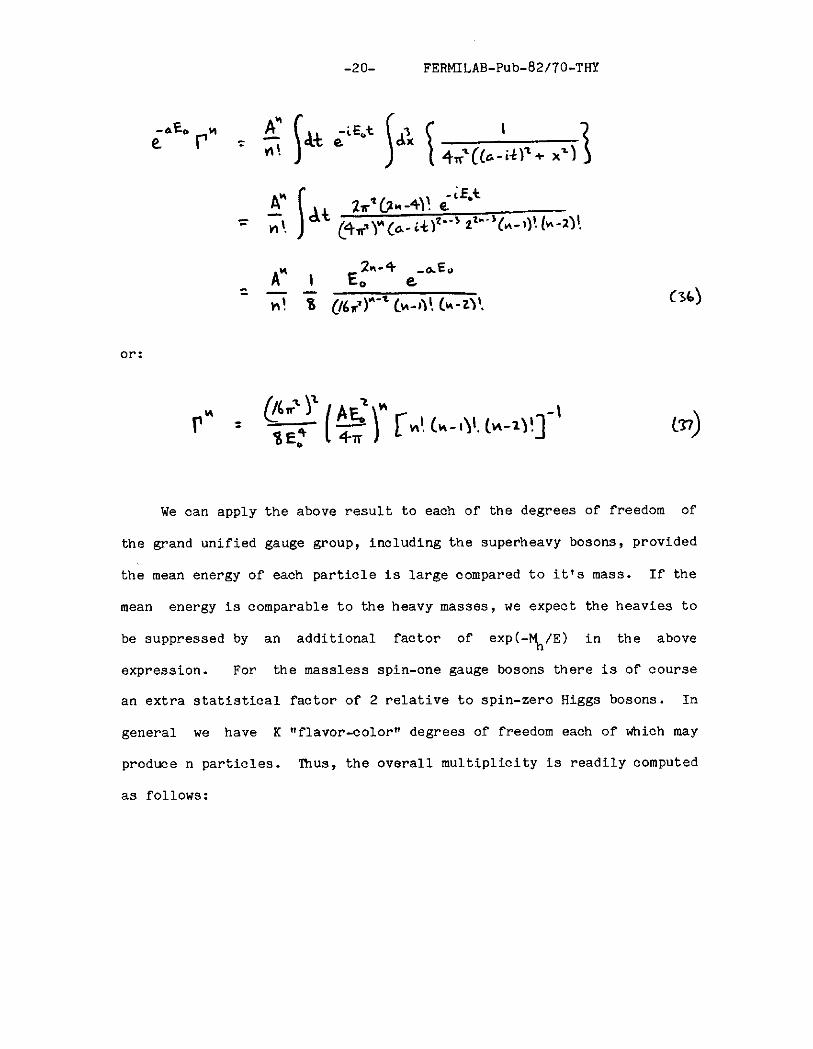
-2o- FERMILAB-Pub-82/70-THY
-oEo e. f5-
2 \A+ eiEot )A% 1 qd((c:it,,+ .%J
-;E.t ?,q(aM-4\? e
= (++j*(& it)+’ P’(H-I)! b-l)!
A~ , E;*-4 /Eu
= n?- 8 (16,)m-a (H-h! (u-a!
or:
p” = (2 [ !$I* Id (H-,)1. (vl-l)!J-’ 0
C36)
We can apply the above result to each of the degrees of freedom of
the grand unified gauge group, including the superheavy bosons, provided
the mean energy of each particle is large compared to it's mass. If the
mean energy is comparable to the heavy masses, we expect the heavies to
be suppressed by an additional factor of exp(-Mb/E) in the above
expression. For the massless spin-one gauge bosons there is of course
an extra statistical factor of 2 relative to spin-zero Higgs bosons. In
general we have K "flavor-color 1' degrees of freedom each of which may
produce n particles. "ihus, the overall multiplicity is readily computed
as follows:
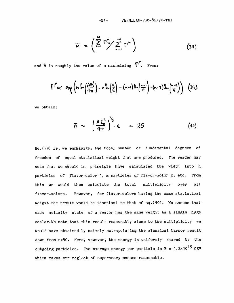
FERMILAB-Pub-82/70-THY
and 'i is rou&ly the value of n maximizing 7". From:
we obtain:
Eq.(39) is, we emphasize, the total number of fundamental degrees of
freedom of equal statistical weight that are produced. lhe reader may
note that we should in principle have calculated the width into n
particles of flavor-color 1, m particles of flavor-color 2, etc. From
this we would then calculate the total multiplicity over all
flavor-colors. However, for flavor-colors having the same statistical
weight the result would be identical to that of eq.(l(O). We assume that
each helicity state of a vector has the same weight as a single Higgs
scalar.We note that this result reasonably close to the multiplicity we
would have obtained by naively extrapolating the classical Larmor result
down from n:40. Here, however, the energy is uniformly shared by the
outgoing particles. The average energy per particle is E : 1.2~10'~ GEV
which makes our neglect of superheavy masses reasonable.

-22- FERMILAB-Pub-82/70-THY
In N(5) we have 24 gauge and 24 Higgs bosons. In counting the
number of X- and Y- bosons we must take a total of 12x2 degrees of
freedom from the gauge bosons and 12x1 (longitudinal) degrees of freedom
from the Higgs. We further have a total of 24x3 degrees of freedom
altogether. Thus the fraction of X- and Y- bosons produced is
12x(2+1)/(24x3)=1/2. mus 25/2 = 12 X- and Y-bosons are expected.
Table(I1) presents the approximate yields and fractions in the burst
phase of the various N(5) gauge and Higgs bosons.
The decays of the superheavy gauge and Higgs bosons as well as the
fragmentation of the gluons will produce very high energy hadron jets as
well has leptons. With an average energy of 0(10'5) GEV the expected
multiplicity par jet is = 10' from the leading log QCD and, though it
somewhat increases the multiplicity at very high energies, it is a
negligible correction to the hadron spectrum of Fig.(3).
The particles produced in the burst will decay into leptons,
quarks, and the lighter gauge and Higgs bosons. Of the 25 degrees of
freedom initially excited, rou&ly 25x2x8/(2x24+24), or ~5 are gluons.
ma remaining 20 objects will typically decay into two body final
states. Ignoring gauge bosons, we expect typically 25% of these will be
leptons and 75% quarks. lhus we get roughly 10 leptons and 30 quark
jets in addition to the 5 original gluon jets. These jets should be
distributed more or less isotropically in space and might be cleanest
along the z-axis of the system where the l-cos2@) Larmor distribution
is zero (of course pT effects and multiple scattering will give a
nonzero background here). me typical jet opening angle at these
energies is("):

-23- FERMILAB-Pub-82/70-THY
k 4 x ,c? Ae$PQS (41)
thus we have very highly collimated jets. We note that even for the
Larmor spin-down the azimuthal distribution of hadrons will not be
entirely uniform. lhe last revolution corresponds to all jets of energy
E > E' where:
*x fir
‘t&-’ = 27r (44
and
thus:
zs ~ 1.2 wJt3 E’- I. 4 x lc? CCL/
E ’
(44)
and the fraction of the full 21razimuthal angle occupied by the hadrons
in jets is:

-24- FERMILAB-Pub-82/'70-THY
$ : :-, @7i’*)&E a .obg rt-1 \
(4-s)
E'
The enormous yield of hadrons would require that to detect the
leading decay fragments of the X-,Y- and superheavy Higgs bosons in a
monopolonium decay event one must be able to cut on all hadrons of
energy less than about 5~10'~ to 1014 GEV and focus upon the very low
multiplicity particles in the 10 14 to 10'6 decades. These objects will
carry the information about the grand unified gauge group. For example,
it may be possible to detect the CP-violation in the decays of
superheavy Higgs (or gauge) bosons by counting a net baryon excess in
the leading particles (expected optimistically at a 10s3 level). mu3
one could test in principle the mechanisms by which the Universe
acquired a net baryon number with q 1000 monopolonium decay events.
Ihis would be extremely difficult at best.
IV. Relic Monopolonium --
The crucial observation of the present section is that, as stated
above, objects of an initial size of order a tenth of an angstrom or
more, have lifetimes equal to or exceeding that of the Universe. mis
suggests the possibility that such monopolonia were formed in the early
Universe and may have survived up to the present. Some fraction of
these will be decaying presently and the high multiplicity of final
fragments may be observable. Alternatively, the larger objects are
presently spinning down and should be producing a diffuse radio
background. From this we can place joint limits on the masses and

-25- FERMILAB-Pub-82/70-THY
closure fractions of arbitrary monopoles as this part of the
annihilation is completely insensitive to the GUT assumption. We will
concentrate presently on the formation of relic monopolonium and leave
many questions of related interest to future discussions (I) .
Our approach will be to give first a very general estimate of the
expected abundance of relic monopolonia from statistical mechanics by
computing the equilibrium fraction of monopolonia at a fixed temperature
in the solution of monopoles and antimonopoles via a
classical-differential version of the Saha equation. mis will
immediately translate into the decay rate in a typical comoving volume.
We will not see in this estimate the specific physical formation
mechanisms, and we shall follow with an estimate based upon a definite
process. Here we will consider the same mechanism by which various
authors have attempted to rid cosmology of an over-abundance of
primordial GUT monopoles. We will look at collisions between "cool"
monopoles and antimonopoles that are hard enou& to capture into loosely
bound states by the emission of classical Larmor radiation. though the
impact of such events upon the background density of free monopoles is
insignificant, nonetheless a substantial abundance of monopolonium is
generated. This specific process will yield a comparable supply to that
suggested by our more general statistical argument.
We see that the binding energy of monopolonia with sizes between
l/IO to 10 Angstrom ranges from q 340 KEV to 3.4 KEV. 'ihus, this is the
relevant temperature scale for the formation and corresponds to the
Universe age of from 10 to 10 4 seconds. We believe we have a reliable
understanding of Cosmology in this epoch since the primordial Helium
abundance can be reliably calculated and agrees with observation. It is
-26- FERMILAB-Pub-82/70-THY
known that for our GUT monopoles, the ratio of the monopole density to
photon density must be less than lo-" during this phase(12), and is
probably at least as small as 10 -24 , since that is the present allowed
fraction given the closure density today and there is no known mechanism
for reliably reducing monopole abundances since that time. Our point of
view is to assume that they must have been in an acceptable abundance
during this epoch and to proceed to obtain essentially a lower limit on
the resulting monopolonium abundance.
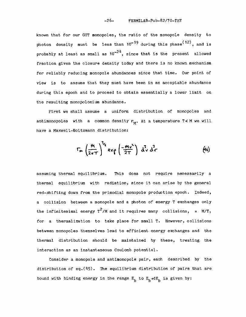
First we shall assume a uniform distribution of monopoles and
antimonopoles with a common density r M. At a temperature T<M we will
have a Maxwell-Boltsmann distribution:
L (&I” exp (-g) .A A?
assuming thermal equilibrium. This does not require necessarily a
thermal equilibrium with radiation, since it can arise by the general
red-shifting down from the primodial monopole production epoch. Indeed,
a collision between a monopole and a photon of energy T exchanges only
the infinitesimal energy T2/M and it requires many collisions, = M/T,
for a thermalization to take place for small T. However, collisions
between monopoles themselves lead to efficient energy exchanges and the
thermal distribution should be maintained by these, treating the
interaction as an instantaneous Coulomb potential.
Consider a monopole and antimonopole pair, each described by the
distribution of eq.(45). lhe equilibrium distribution of pairs that are
bound with binding energy in the range Eb to Eb+dEb is given by:

-27- FERMILAB-Pub-82/70-THY
-; Mv: - &MY,’ + +h - r,l
T
* b(E b - ;iii(“,-f*y:, - y&d) k c,ri 147)
It is convenient to go over to center of mass positions and velocities,
v=(vl+v2)/2, u=(v,-v2), R=(r,+r2)/2, r=(r,-r2):
$VcfRd~d’: exf (-‘&&&$+ &)
. $,(-\E&f%+ $1 hEb cmrc
: 2M ‘5 ( )I 2rrT d3v a7 es{ (-I mv: 4) &&
where the result has been factorized into a Maxwell-Boltzmann
distribution in the boundstate with mass 2M times the density fraction
of the boundstates in the background monopole anti-monopole gas:
& d’r g- \fJ - y+ +, Q -($Y 2))
r, c,- hEb (47)
Performing the d3u integration gives:
ck,g = + - ~k.lj:itJhcarg b:AE, [so)

-28- FERMILAB-Pub-82/'70-THY
'fnus, performing the y integral gives:
dq& = 2 ( g, [+J-& hfb”ym (4
lhis is simply a classical version of the Saha equation, which may be
viewed as formation by multibody monopole collisions in thermal
equilibrium. In a comoving volume we have NM monopoles. We may write:
r, = CL? (rk/rJ cl= q30
Thus the number of boundstates in the comoving volume with binding
energy Eb to Eb+dEb becomes:
ANI, = $y ($) ( &bre’Eb’iT$ NM (E) (s4)
me ratio rM/rx is cosmologically invariant for the low formation rates
discussed here.
-2% FERMILAB-Pub-82/'70-THY
We see that the binding energy enters an exponential and thus the
most probable states by eq.(54) have infinite binding energy. lhis is
the well known disease of the Coulomb gas and it is readily interpreted.
In general, as the members of a pair get very close together the
Boltzmann factor in eq.(47) is diverging. But such a pair is also no
longer in thermal equilibrium and is dominated by the local mutual
Coulomb force. Only when the energy is within an order of magnitude of
the temperature is the process expected to be reliably described as an
equilibrium one. lhus we may only apply eq.(54) for E : 7T, where '2
is a parameter of O(1). Thus we have for the differential number of
objects instantaneously bound with energy E to E+dE:
hNU, = 2 [&$eq $. N- (z) CSS)
where N m is the number of monopoles in a comoving volume.
Strictly speaking, these objects are not bona-fide boundstates, but
only thermal fluctuations of an arbitrary pair into a state of locally
negative total energy. lhey are the equilibrium fraction of the
monopolonia dissolved in the monopole anti-monopole gas. However, as
the system cools we expect that for an appropriate choice of -O(l) this r
abundance of objects will be left behind as boundstates since their
binding energy will exceed the thermal energy available to dissociate
them. Lexus eq.(55) is indeed expected to describe the relic abundance
of monopolonia formed as the Universe cooled through a temperature of
order the binding energy.

-3o- FERMILAB-Pub-82/70-THY
The formula of eq.(55) possesses a pleasant scaling behavior.
Reference to the lifetime formula of eq.(12) shows that we may write:
mus, the decay rate of monopolonia in a comoving volume follows
immediately:
Ma; TG= -: [&k.fQy~) (57)
We see that the decay rate increases as the age of the comoving volume
decreases. Today, a typical cubic light-year would contain roughly
3x10e3' GUT monopoles if we saturate the closure density. From eq.(57)
we obtain-350 decays of monopolonia per year per cubic light-year,
assuming the conservative r /r q -24
M$ 10 , and 3.5~10" saturating the
Helium abundance limit of rM/rV = 10-l'. We may further estimate the
total fraction of monopolonia by converting from lifetime to diameter
through the convenient scaling law:
CSd
Thus, we may integrate from a radius of r : l/10 Angstrom up to an upper
limit, R, for which we expect the formation to terminate:

-31- FERMILAB-Pub-82/70-THY
We thus see that the specific choice of R is irrelevant as we are only
logarithmically sensitive to it. In practice we would expect R to
correspond to a value for which a monopolonium is readily ionized by a
magnetic field or other traumatizing event (we note that at l/10 A it
requires a B-field of order 10" Gauss to ionize). Putting in numbers
yields about 10" (or 10" assuming the larger monopole to photon ratio)
GUT monopolonia per cubic li@at year, or a fraction of 10 -18 monopolonia
to monopoles.
In fact, we expect that eq.(59) with 7'
1 probably underestimates
the abundance of monopolonium since it makes no reference to specific
reactions such as capture by the emission of radiation, scalars or other
particles, and considers only monopole collisions in thermal equilibrium
implicitly via their instantaneous Coulomb potential. We may directly
estimate the formation of monopolonium by radiative capture essentially
making use of the cross-section:
Cdr> = T(+$j$($\
where the quantity in braces is familiar (12) , but we've obtained the
extra overall numerical factor z9.6. E. is the kinetic energy of an
incident monopole at infinity which is of order the temperature (it
would be a straightforward analysis to fold in the complete thermal
distribution here). This follows by demanding a classical collision

-32- FERMILAB-Pub-82/70-THY
between monopole and anti-monopole during which there is sufficient
acceleration to radiate away the energy by the Larmor power formula.. In
fact, we may use more general differential cross-section:
d C& > A%
= 9.6$ L ) (61)
which is the cross-section of capture into boundstates of binding energy
Eb' me rate of
temperature T in a.
formation of monopolonia into these states at
given comoving volume is:
= (33) @) (t)” ( T;,Ebr( $y ““” (62)
We may convert the differential formation rate in time into a rate
in temperature in a comoving volume (thus the Hubble expansion terms do
not appear). 'Ihis may be integrated over all temperatures and we note
that the integral receives most of it's contribution for T : Eb as
expected. lhe result is:

-33- FERMILAB-Rub-82/70-THY
(63)
9 c = i (4 bosor Irdicikt~ + i t, &w;‘., \\c\;r;\isr)
where the integral is:
00
13 I
A* x”l (\ + x )7’S % 2.2
0
lhe final monopolonium abundance is numerically:
N- $1 rv 2o.g c$” wypp
( ~y/,o [EbP (5%) m ,o@ rv
(65)
and we have the decay rate:
mis is remarkably close to our preceding result even though it involves
somewhat different physics. me exponent 9/10 is sufficiently close to
unity that our scaling is approximately valid as well. me rough
agreement between these results encourages us that they are probably
correct thou@ a more detailed analysis of specific mechanisms is
desired. Moreover, perhaps our choice of 7’ 1 in eq.(57) is overly

-34- FERMILAB-Pub-82/70-THY
restrictive. If
256'=
10 the rates and fractions are increased by a large
factor of , and as 1 -
>60 all monopoles become bound into
monopolonia. We can envision a number of additional mechanisms that
might significantly enhance the formation rates and we regard the quoted
results as probable lower limits on the formation.
We will not give here a detailed description of the observability
of relic monopolonium. However we will remark that we can place
nontrivial limits on the monopole masses and closure fractions from the
above considerations and that we believe that the decay products of
these systems mi@t be detectable in a variety of experimental
configurations. A systematic discussion of the observational
implications, constraints, signatures and other general considerations
is in preparation(').
Acknowledgements
I have greatly benefitted from discussions with Prof. J.D.
Bjorken with whom many of these ideas were initially developed. Also,
Prof. D. Sohramm has contributed in developing the cosmological
arguments. I have also benefitted from discussions with Prof. W.A.
Bardeen, Prof. J. Ostriker, Prof. J. Rosner and Dr. R. Orava.
1.
2.
3.
4.
5.
6.
7.
8.
9.
-35- FERMILAB-Pub-82/70-THY
References
C. T. Hill and D. Schramm, in preparation
of related interest is: F. Bais, P. Langacker, Nucl.Pnys. B197, (1982) 520
V. A. Rubakov, Nucl. mys. B203 (1982) 311; C. G. Callan, Princeton University Preprints, "Disappearing Dyons" and "Dyon Fermion Dynamics"
c. P. Dokos, T. N. Tomaras, Pays. Rev. D21 (1980) 2940; M. Daniel, G. Lazarides, Q. Shafi, Nucl. Phys. B170 (1980) 151
S. Coleman, 1981 Int'l School of Subnuclear physics, "Ettore Ma. j oranan
J. D. Jackson, Classical Electrodynamics, J. Wiley & Sons, N. Y., (1963)
A. H. Mueller, pnys. Lett. 104B (1981) 161; A. Bassetto, M. Ciafaloni and G. Marchensini, Nucl. mys. B163 (1982) 477; A. H. Mueller, Columbia University Preprint, Cot. 1982
See e.g., K. H. Mess, B. H. Wiik, Desy 82-011 (1982) for a review
D. Horn, F. Zachariasen, Hadron Physics at Very High Energies, W. A. Benjamin, Reading, Mass., (1973)
10. J. D. Bjorken, S. Brodsky, Whys. Rev. Dl (1970) 1416
11. G. Sterman, S. Weinberg, Whys. Lett., 39 (1977) 1436
12. J. Preskill, Fhys. Rev. Lett. '9, (1979) 1365

FIGURE CAPTIONS
Fig. 1 Normalized probabilities, p y' PzO' pgluon'
Fig. 2 Y,ZO , gluon d(ln(n)ld(ln E)vs. (ln E.)
Fig. 3 Charged Hadron spectrum (a) leading lo!3 QCD,
(b) E1'2 multiplicity, and (c) gluon spectrum.
y-distribution S l/3 hadron distribution.

Table 1. Monopolonium Properties
Classical Lifetime Binding Transition Principal Diameter hemy Energy Quantum
(cm) (see) (GeV) (eV) Number v/c
lo-*
10-g
IO-IO
lo-"
lo-l2
lo-l3
lo-l4
10 -15
10-16
lo-'*
lo-2o
lo-22
lo-24
10-26
lo-28
3.71x10²²
3.71x10'*
3.71x10¹⁵
3.7lxlo12
3.71x10⁹
3.71x10⁶
3.71x10³
3.71
3.71x10⁻³
3.71x10⁻⁹
3.71x10-'5
3.7lxlo-21
3.71xlo-27
3.71x10⁻³³
3.71x10-39
3.35x10⁻⁵
3.35x1o-4
3.35x10⁻³
3.35xlo-2
3.35x10-l
3.35
3.35x10'
3.35x10²
3.35x10³
3.35x10⁵
3.35x10⁷
3.35x10⁹
3.35x10"
3.35x10'3
3.35x10¹⁵
1.61x10-~
5.o9xlo-6
1.61~10 -4
5.o9x1o-3
1.61x10-'
5.09
1.61~10~
5.09 x10³
1.61~10~
1.61x10*
1.61x10"
1.61~10'~
1.61~10 17
1.61~10~~
1.61~10~~
4.17x10"
1.32~10"
4.17xlo'"
l.32xlo'"
4.17x10⁹
1.32~10~
4.17x10*
,.32x10*
4.17x107
4.17x10⁶
4.17x10⁵
4.17x10⁴
4.17x10³
4.17X10²
4.17x10'
4.10x10-"
l.30xlo-'"
4.10xlo-'"
1.30x10⁻⁹
4.10x10-*
1.30x10 -a
4.1ox1o-8
1.30x10 -7
4.10x10⁻⁷
4.10x10⁻⁶
4.10x10-'5
4.10x10 -4
4.10x10⁻³
4.1oxlo-2
4.10x10-'

Table 2. Fractions and Approximate Yields in Burst
Species Fraction Approx. Yield
X,E l/4 6
Y,P l/4 6
w+,w- ZO l/12 2
gluons 219 6
Y l/36 0
color 8
>
l/9 3 Higgs
weak
>
T/24 1 Higgs
5 0 cl-- 2 a” . . . I . . I
. . . . . . . . . . . . . . . . . . . . . . . . .
-3 i I
42
4
oi.2 * -c-u- -
t 2 -
-In

I I I I I I I I I
. . : . . . . . .
/
. . l:: .
!(: SGi ;;i 2- ON i;j X- OC
-ETl
-g.g 6”
-0 Q
f
/f : .
I I J: I’ I
I.’ Se
C u cl .- E:: -7 m E 2 ‘z F” -- .-
c! -0 5 -w - r ::
. . . I . . . I .
l .** , / I l 1
. . / . / I
. . . . / / . . . . . . I I 9 I I I I I I I I I
0
2 25 : “0 3
2 =C -0 u
RGj ~ m
- . c LY -
h
2


![Untitled3 [lss.fnal.gov]lss.fnal.gov/archive/other/sdc/sdc-90-151.pdf · 2009. 8. 12. · SD~-'tO-OO,s-l Or Letter of Intent OT by the SOLENOIDAL DETECTOR COLLABORATION to construct](https://img.dokumen.tips/doc/110x75/5fd2004678236530e445a345/untitled3-lssfnalgovlssfnalgovarchiveothersdcsdc-90-151pdf-2009-8.jpg)