Monopolistic Competition in Electricity Networks with

Resistance Losses∗

Juan F. Escobar†

Stanford University

Alejandro Jofre‡

Universidad de Chile

August 07, 2008

Abstract

We consider a pool type electricity market in which generators bid prices in a sealed bid

form and are dispatched by an independent system operator (ISO). In our model, demand

is inelastic and the ISO allocates production to minimize the system costs while considering

the transmission constraints. In a departure from received literature, the model incorporates

explicit description of the network details. The analysis shows that losses along transmission

lines render the market imperfectly competitive. Indeed, it is shown that competition among

generators is qualitatively similar to the interaction among firms in a monopolistic competition

setting. A lower bound for market prices is derived and it is shown that the costumers’ cost

of oligopolistic pricing is strictly positive. At a methodological level, we generalize standard

oligopoly theory tools.

∗We would like to thank to Soledad Arellano, Sophie Bade, Ross Baldick, Alex Galetovic, Aldo Gonzalez, Rodrigo

Palma, Robert Wilson, and several seminar participants for useful suggestions. We particularly thank two anonymous

referees for their detailed review and suggestions. Anne-Lise Thouroud provided helpful research assistance. This

work was partially supported by ICM Complex Engineering Systems.†Department of Economics, Stanford University. 579 Serra Mall, Landau Economics Building, Stanford, CA

94305. Email: jescobar@stanford.edu.‡Depto de Ingenierıa Matematica and Centro de Modelamiento Matematico, Universidad de Chile. Blanco En-

calada 2120 7o. piso, Casilla 170/3 Santiago de Chile. Email: ajofre@dim.uchile.cl

1

Keywords: electricity networks, transmission losses, spot markets, monopolistic competition,

oligopoly theory, stability analysis.

JEL Classification: C61, D43, L94.

2

1 Introduction

A particularly common design in recently liberalized electricity markets organizes wholesale trading

through an integrated market. In those markets, wholesale generators and costumers participate in

a sequence of auctions. A central authority, hereafter referred to as independent system operator

(ISO), coordinates the market participants with the purpose of optimizing the system operations.

Examples of this organization can be found increasingly in the US, as well as in Colombia, Spain,

and the UK.1

A key aspect differentiates wholesale electricity markets from virtually any other market, namely,

electricity transfers take place on electricity grids, and electricity grids have a complex physics. In-

deed, electricity transfers must respect transmission and generation constraints, Kirchhoff’s laws,

and unexpected network failures. The importance of network constraints on market outcomes has

been recognized by several authors.2 Indeed, network constraints may allow some generator to

exercise market power even in the presence of several potential competitors. However, the analyt-

ical frameworks provided by existing models to understand the consequences of realistic network

constraints on pricing strategies are limited in several aspects (we review the received literature

below).

The present paper models a bid based integrated power market that functions on an arbitrary

electricity network. In our model, generators submit prices in a sealed bid form and prices cannot

be higher than the exogenously set price cap. The ISO uses the bids to represent the system costs

and allocates production among generation units in order to minimize the social cost of serving total

demand. The model includes explicit description of the network details and their consequences on

feasible allocations. We focus on the noncooperative outcome of the game among generators.

It is first shown that the interaction among generators can be understood in terms of standard

economics. In fact, as a consequence of transmission losses along transmission lines, the game

among generators is qualitatively similar to the interaction among firms facing Hicksian demands

in a monopolistic competition setting. So, while the game analyzed becomes a first price auction in

the no network case, the existence of transmission losses makes the game a competition in differ-

entiated products. A simple two-generator example illustrates how the magnitude of transmission

losses determines the intensity of market competition, ranging from homogenous product Bertrand

competition in the no losses case to purely monopolistic pricing when losses are sufficiently large.

1See Wilson (2002) for additional details.2For example, Borenstein et al. (2000) emphasize that “transmission constraints will be at the heart of market

power issues in a restructured electricity market.”

3

While useful, the monopolistic competition analogy does not permit us to immediately derive es-

timates of equilibrium outcomes. To do that, the main difficulty is the intrinsic non-differentiability

of each generator’s maximization problem (whose origin is precisely the presence of network con-

straints); we therefore carry out a quantitative stability analysis of the dispatch program to derive

estimates of demand functions’ slopes. Then, a lower bound for the markup that each generator

sets is derived in terms of the network fundamentals. This bound shows that no matter the fine

details of the network, whenever a generator expects to be dispatched at some positive quantity, it

exercises market power and raises its bid above its marginal cost. As a consequence, consumers’

cost of oligopolistic pricing is strictly positive.

Though the presence of transmission losses is key at driving our results, in practice they may be

quite modest. Notwithstanding, their importance on market prices may be significant and indeed it

may compare to the impact of congestion on prices.3 As a consequence, the introduction of trans-

mission losses not only facilitates the analysis by “smoothing out” the model,4 but understanding

its impact on pricing strategies is an interesting question by itself.

Prices above marginal costs echo the conclusions of previous works. However, our argument

relies on a feature –namely the product differentiation pushed by the physics of power flows– that

has not been formally captured by previous models and applies to a large set of electricity networks.

We explore a few examples to assess the gap between actual equilibrium prices and the lower

bound. These examples show that the bound may bind, may provide a good approximation, or

may be vaguely informative about equilibrium prices.

The methodology employed to analyze the model constitutes an additional contribution of this

work. We borrow some tools from optimization theory, and study different stability concepts for

minimization problems. Our approach contrasts with the standard framework for strategic competi-

tion on networks, which relies on properties for (convex and/or differentiable) variational inequalities

and mixed complementarity problems. We view our methodology as a natural generalization of some

techniques employed in oligopoly theory. New applications may arise in oligopoly models where de-

mand functions are derived from complex optimization problems, as in Hotelling competition in

several dimensions, or consumer problems with constrained decision sets.

Related Literature. This paper pertains to two strands of the economics literature on

electricity markets. The first one analyzes the impact of generators’ strategies in N -firm power

3CAISO’s studies illustrate this point. See, for example, Table 1 in the August 2004 analysis of market-based

price differentials at http://www.caiso.com/17ea/17eacf356fab0.pdf. We thank a referee for bringing this reference

to our attention.4Our lower bound allow us to estimate the impact of virtually any other network constraint on market prices.

4

pools on market outcomes. Green and Newbery (1992), in a pioneer work, model the British

pool adapting the supply function equilibrium model introduced by Klemperer and Meyer (1989).

Generalizations and extensions of Green and Newbery’s model are given by Green (1999), and

Newbery (1998). On the other hand, von der Fehr and Harbord (1993) do not smooth the bids

and model the UK electricity pool as a first-price multi-unit auction. Fabra et al. (2006) analyze

different auction formats for bid based pools. All of these models ignore the complexity of power

transfers and analyze competition among generators not considering the transmission network as a

potential source of market power.

A second set of works explicitly models the effects of network constraints on market outcomes.

Borenstein et al. (2000) show that the competitive impact of small transmission lines may be

important, while Joscow and Tirole (2000) emphasize the role of the structure of transmission rights.

These authors model competition a la Cournot on small two-node networks. While these models

are particularly tractable, the generality of the insights obtained is rather limited. Additionally, in

these works market power is the consequence of binding transmission capacities. In contrast, in our

model market power arises as a result of the intrinsic physics of power transfers.5

Since our model can be seen as a Hotelling-type model of monopolistic competition, this paper

also relates to spatial competition models (e.g. Hotelling (1929), D’Aspremont et al. (1979), Hobbs

(1986), Anderson et al. (1989), Mulligan and Fik (1994)). We contribute to this literature by adding

a network to the analysis and deriving the differentiation among firms from network fundamentals.

The methodology introduced to analyze the (non-differentiable) game among generators could also

be exploited in other Hotelling-type models.

Variational inequalities have proven useful to study power markets. Wei and Smeers (1999),

for example, model the long-term interaction among firms which build capacities and commit their

outputs (Day et al. (2002) and Pang and Hobbs (2004) offer interesting generalizations). Hobbs et

al. (2000) formulate the problem of finding a power market equilibrium as a mathematical program

with equilibrium constraints. Ehrenmann and Neuhoff (2004) study a market design similar to the

one studied in this paper and compare it to an unbundled system. These works address the problem

of computation of equilibrium in pure strategies (which not always exist). More closely related to

the present work, Hu and Ralph (2007) study the problem of pure strategy existence in a model

similar to ours.

5More recently, Cho (2003) provides welfare theorems for a network market. In Cho’s model, the physical

environment in which agents interact is considerable more complex than Borenstein et al.’s. Yet Cho restricts

participants’ sophistication and studies the competitive equilibrium of the market. The present paper not only

permits a more general network structure but also focuses on the more realistic case of strategic interaction.

5

The Rest of the Paper. Section 2 gives a simple illustration of some of our results. Section

3 presents our general model, and introduces definitions, notation, and assumptions. Section 4

presents and exemplifies our results. Section 4 additionally discusses some extensions. Section 5

presents some final remarks. Supporting material and proofs are presented in the Appendix.

2 An Example

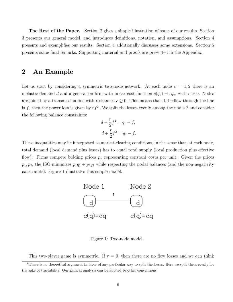
Let us start by considering a symmetric two-node network. At each node v = 1, 2 there is an

inelastic demand d and a generation firm with linear cost function c(qv) = cqv, with c > 0. Nodes

are joined by a transmission line with resistance r ≥ 0. This means that if the flow through the line

is f , then the power loss is given by rf 2. We split the losses evenly among the nodes,6 and consider

the following balance constraints:

d+r

2f 2 = q1 + f,

d+r

2f 2 = q2 − f.

These inequalities may be interpreted as market-clearing conditions, in the sense that, at each node,

total demand (local demand plus losses) has to equal total supply (local production plus effective

flow). Firms compete bidding prices pv representing constant costs per unit. Given the prices

p1, p2, the ISO minimizes p1q1 + p2q2 while respecting the nodal balances (and the non-negativity

constraints). Figure 1 illustrates this simple model.

Figure 1: Two-node model.

This two-player game is symmetric. If r = 0, then there are no flow losses and we can think

6There is no theoretical argument in favor of any particular way to split the losses. Here we split them evenly for

the sake of tractability. Our general analysis can be applied to other conventions.

6

of the network as consisting of a single node. The game is just an homogenous product Bertrand

game and generators bid prices that equal their marginal costs c. No market power is exercised.

Things are different when r > 0. In this case the marginal cost of power from generator 2 at

node 1 is a strictly increasing function (and, of course, so is the marginal cost of power at node

2 from generator 1). Then, if generator 1 increases its bid a little, the quantity at which it is

dispatched is just slightly smaller. Consequently, each generator faces a continuous non increasing

demand function. Indeed, in the Appendix, it is shown that the quantities at which generators are

dispatched are

Q1(p1, p2) = d+1

2r(p2 − p1

p2 + p1

)2 +1

r(p2 − p1

p2 + p1

), Q2(p1, p2) = d+1

2r(p1 − p2

p2 + p1

)2 +1

r(p1 − p2

p2 + p1

).

Consequently, the game can be seen as a Bertrand competition model with differentiated products.

It should not be surprising that generators are able to exercise market power. In fact, it is not

hard to see that∂Q1(p1, p2)

∂p1

= −1

r

4p21

(p1 + p2)3

and therefore the necessary optimality condition for a symmetric equilibrium p = p1 = p2 is (p −c)1r

4p2

4p3= d. The only solution to this equation is p = c/(1 − 2dr) and indeed constitutes an

equilibrium (see Appendix for details). Firms bid strictly above marginal costs, c, and there is no

power flow along the transmission line. The very existence of transmission losses enables generators

to set higher prices.7

In this model, market power has nothing to do with binding constraints. This contrasts with

previous works where the source of network-driven market power is either generation or transmission

constraints (e.g. von der Fehr and Harbord (1993), Borenstein et al. (2000)). In this sense, market

power is structural: regardless of the installed capacity and the details of the transmission network,

prices will be above marginal costs.

3 The General Model

Now we present a general version of the simple two-node model introduced in the previous section.

Consider an oriented connected graph (V,E), where V is the set of vertexes and E is the set of edges.

Each vertex v ∈ V is a network node. Each edge e ∈ E represents a high-voltage transmission line.

7 In fact, in this two-node model transmission losses play a role similar to that of transportation costs in a

Hotelling model.

7

There is only one generator at each node v ∈ G, where G ⊆ V . Each node v ∈ V has an inelastic

demand dv ≥ 0.

Generators bid, in a sealed bid form, prices pv ∈ [0, p∗], where p∗ is an exogenously defined price

cap. After knowing the vector of bids p = (pv)v∈G, the ISO minimizes the overall cost∑

v∈G pvqv

of serving the (inelastic) market demands by determining the quantities q = (qv)v ∈ RG that the

generators produce and managing the flows f = (fe)e ∈ RE over transmission lines.

Not every tuple (f, q) is feasible, however. One of the main innovations of the present work is the

explicit consideration of network constraints. These network constraints, which must be respected

by the dispatch process, are detailed below.

Nodal Balances. At each node, available power must satisfy nodal demand. There are power flow

losses in the transmission lines. A well known way to approximate losses is as a quadratic functions.

Indeed, if the flow over e ∈ E is fe, the loss is given by ref2e , where re ≥ 0 is the line resistance.

Assuming that losses are split between the nodes associated to each line, the nodal power balances

are8 ∑e∈Kv

re2f 2e + dv = qv +

∑e∈Kv

fesgn(e, v), v ∈ G (3.1)

∑e∈Kv

re2f 2e + dv =

∑e∈Kv

fesgn(e, v), v ∈ V \G, (3.2)

where Kv is the set of transmission lines connecting node v and sgn(e, v) is equal to 1 or -1 depending

on the orientation of the graph and whenever e = (v, w), sgn(e, v) = −sgn(e, w). We also denote

K = ∪v∈GKv. The left hand side of (3.1) is half the sum of all the losses related to node v plus

nodal demand dv. The right hand side of (3.1) is the production of generator v plus the sum of

effective flows.

Generation Constraints. Each generator has a nonempty production set

qv ∈ [0, qv], (3.3)

where qv ≥ 0.

Transmission Constraints. Each transmission line e ∈ E has a maximum safe capacity:

fe≤ fe ≤ f e, where f

e≤ 0 ≤ f e. More generally, we consider the constraint

f ∈ F, (3.4)

8Under our working assumption (A2), these equalities could also be written as inequalities that turn out to bind.

This is not always the case; see, for example, Chao and Peck (1996)

8

where F ⊂ RE is a convex compact set. This formulation is general enough as to include Kirchhoff’s

voltage law constraints and other network constraints.9

We denote by Ω the set of pairs (f, q) ∈ RE × RG satisfying (3.1)-(3.2)-(3.3)-(3.4). We assume

that Ω is nonempty.

After knowing the bids p = (pv)v∈G, the ISO runs the following dispatch program

min∑v∈G

pvqv | (f, q) ∈ Ω. (3.5)

In words, the ISO optimizes the system operations as if the auction prices were generators’ marginal

costs. Of course, in practice this needs not be so for generators could game the dispatch process to

maximize their profits.

We define OPT (p) = min∑

v∈G pvqv | (f, q) ∈ Ω and the set

Q(p) = q ∈ RG | ∃f ∈ RE, (f, q) is a solution of (3.5)

of optimally generated quantities q = (qv). This set is nonempty and compact.

Generator v’s payoff depends on the quantity at which it is dispatched and the clearing price at

its node. When bids are p = (pv)v∈G and the dispatch is q ∈ Q(p), the payoff for generator v is

uv(pv, qv) = pvqv − cv(qv), (3.6)

where cv is a real-valued cost function.

We are interested in the noncooperative outcome of this game. To be more precise, an equi-

librium is a tuple of distributions (Fv)v∈G with supports contained in [0, p∗], such that for some

selection q(p) ∈ Q(p), p ∈ [0, p∗]|G|, given the dispatch rule q, no generator can improve its expected

payoff by unilaterally modifying its prescribed distribution Fv.

In the sequel, we consider the following realistic assumption.

A1 (a) Existence of transmission losses: For all e ∈ E, re > 0;

(b) Existence of demand: For some v, dv > 0.

For v ∈ G and a vector of flows fKv ∈ RKv representing flows along transmission lines connecting

node v, consider

Tv(fKv) :=∑e∈Kv

re2f 2e + dv −

∑e∈Kv

fesgn(e, v).

We make the following assumption on the network.

9Kirchhoff’s voltage law: change in voltage over any loop is equal to zero. See Schweppe et al. (1988).

9

A2 For all f ∈ F and all v ∈ G, Tv(fKv) ≥ 0.

This condition restricts the structure of the electricity network; however it should not be deemed

as particularly demanding. For example, it holds if at each node v ∈ G, dv = 0, and v is connected

by only one transmission line to the electricity network.

We also make the following assumption on firms’ costs.

A3 For all v, cv is convex and continuously differentiable and its derivative at 0, c′v(0) = limy→0cv(y)−cv(0)

y,

is strictly positive.

Assumption (A3) implies that each firm is willing to produce a positive quantity only if the per

unit price is strictly positive.

4 Analysis

4.1 Preliminary Results: Product Differentiation and Equilibrium Ex-

istence

We begin by proving the following important and simple lemma.

Lemma 1 If for all v, pv > 0, then Q(p) is a singleton. Moreover Q(·) is continuous on ]0, p∗]|G|.

This lemma formally states that in our model competition is in differentiated products. At first

glance, this property may not seem intuitive. Indeed, if the dispatch process were unconstrained,

the whole market demand would be allocated to the generator bidding the lowest price. In this

case, as usual in homogenous Bertrand games, a discontinuity unambiguously appears when two or

more generators bid the same price. The key assumption allowing us to prove this continuity result

is the existence of transmission losses. The intuition for this result has already been presented in

Section 2.

It is natural to interpret the dispatch program as a minimum expenditure problem and the

tuple (Qv)v∈G : [0, p∗]|G| → R|G|+ as Hicksian demands. Moreover, by employing necessary optimality

conditions, it is not hard to show that the demand system (Qv)v∈G satisfies a law of demand.

Since our game is qualitatively similar to a Bertrand game with differentiated products, the

existence of equilibrium can be analyzed using standard tools. Moreover, the equilibrium can be

taken symmetric if the network and cost functions have a symmetric structure.

10

Proposition 2 There exist distributions (Fv)v∈V that form an equilibrium.

Note that in the standard first price auction, payoff functions are discontinuous and therefore

existence cannot be ensured by employing straightforward fixed point arguments. While our game

becomes a first price auction in the no network case, the existence of network constraints greatly

simplifies the existence proof. Ensuring existence in pure strategies is hard because generators’

payoffs are non-convex; we get back to this point in Section 4.4.

Because there are many complex network constraints, it is not possible to establish the kind of

complementarity exhibited by the functions (Qv)v∈G. Furthermore, the demand functions (Qv) are

not differentiable even in simple networks. We therefore need to introduce new tools to understand

more fully the interaction among generators.

4.2 Main Results: The Exercise and Cost of Market Power

The main purpose of this subsection is to provide a lower bound for the markup set by each generator

in equilibrium and estimate the social cost of oligopolistic pricing. In order to derive those results,

the following result is key; see the Appendix for a proof.

Proposition 3 Take a profile p ∈]0, p∗]|G| and fix a generator w ∈ G. Consider pw ∈]0, p∗] such

that pw − pw is small enough. Then,

|Qw(p)−Qw(pw, p−w)| ≤ |pw − pw|(|Kw|(1 + maxe∈Kw re maxf e, |f e|

)2

σ,

where σ = 12

minv∈Gpv(mine∈Kv re).

Proposition 3 shows that the demand system depends Lipschitz continuously on bids.10 The

result provides an estimate of the slope of the demand function faced by each generator and therefore

it will be useful to study the trade-off each generator solves when bidding. To see intuitively why

differentiability of the demand system cannot obtain, note that in the presence of several constraints,

the solution of an optimization problem will typically be defined by parts. So, the solution exhibits

several kinks and therefore will not be differentiable in general.

10 Milgrom and Segal (2002) study differentiability properties of the value of a parameterized family of optimization

programs. In a departure from those envelope results, we are interested in regularity results for optimization problems

in terms of the set of optimal solutions.

11

So far we have not analyzed whether equilibrium prices will be inefficiently high. We recall

that the standard way to answer that question in Bertrand games with differentiated products is

to derive first order conditions for each player’s maximization problem. This approach cannot be

followed in our general model for demand functions are not differentiable. However, the Lipschitz

property stated above allows us to give an estimation of equilibrium markups.

Proposition 4 Define the payoff that w obtains at equilibrium by playing the pure strategy price

pw as

αw(pw) = Ep−w [uw(pw, Qw(pw, p−w))] =

∫uw(pw, Qw(pw, p−w))dF−w(p−w),

where Ep−w is the expectation with respect to the product distribution∏

v 6=w Fv and uw is defined in

Equation (3.6). Take pw maximizing αw over [0, p∗].11 Then, either pw = p∗ or

Ep−w |pw − c′w(Qw(p))| ≥Ep−w [Qw(pw, p−w)]

ηw(4.1)

where

ηw = 2|Kw|2

(1 + maxre maxf e, |f e| | e ∈ Kw

)2

minv∈Gc′v(0)(mine∈Kv re).

If generator w has a linear cost function, cw(q) = cwq, then

pw − cw ≥Ep−w [Qw(pw, p−w)]

ηw. (4.2)

To prove this result we establish an optimality-like condition for generator w’s maximization

problem. Such optimality-like condition can be derived since Proposition 3 provides an estimate

for the slope of the demand function.

A consequence of the result above is that each generator raises its price above marginal costs

whenever it is dispatched with positive (but eventually small) probability. That can happen, for

example, because the generator is a big producer or because the network isolates it with some

demand (see also Example 6). On the other hand, if the generator bids prices close to its marginal

costs, then it expects to be dispatched at a low quantity. More generally, the impact of any network

constraint on market prices can be estimated by its effect on quantities normalized by a slope term;

see Subsection 4.3.

We can interpret ηw as a measure of the slope of the demand function faced by w. Roughly

speaking, the greater ηw, the more elastic the demand function that the generator faces and the

more aggressive its behavior.

11Note that, in general, the equilibrium may be in mixed strategies. In any mixed strategy equilibrium, generator

w chooses prices that maximize αw(pw) with probability 1.

12

The market outcome may or may not be efficient. For example, in the only equilibrium of the

symmetric generator model analyzed in Section 2, production is efficient. However, the consumers’

cost of market power is strictly positive, as stated in the following result.

Corollary 5 Under the assumptions of Proposition 4, suppose additionally that for all v, cv(qv) =

cvqv. Denote c = (cv)v∈G. Then, for any equilibrium distribution F and any price p in the support

of F there exists κ(p) ≥ 0, such that

OPT (p) ≥ OPT (c) + κ(p).

Moreover, defining ψ(p) = (ψv(pv))v∈G by ψv(pv) =Ep−v [Qv(p)]

ηv,

κ(p) = OPT (ψ(p)),

and it is strictly positive provided all players expect to be dispatched at positive quantities given p.

4.3 Examples

In this subsection we illustrate our results. We start by showing the impact of capacity constraints

on market prices. This reasoning could be used to carry out a variety of comparative statics exercises

(for example, an increase in transmission losses).

Example 6 (Exploiting generation constraints) Any feasible pair (f, q) satisfies∑v∈G

qv ≥∑v∈V

dv +∑e∈E

ref2e ≥

∑v∈V

dv. (4.3)

Therefore, for all w

qw ≥∑v∈V

dv −∑

v∈G,v 6=w

qv.

Assuming costs are linear,

pw − cw ≥∑

v∈V dv −∑

v∈G,v 6=w qv

ηw.

This expression shows how total demand impacts markets’ pricing. In particular, it shows that if

total network demand∑

v∈V dv increases sufficiently, then the distribution of market prices will get

closer and closer to the price cap and the bound will eventually bind.12

12This (formal) result is not obvious. It would be possible that the network isolates some generator and the demand

increase could take place far away from that generator. The generator still will bid close to the price cap because

the network is connected and, at some demand level, the ISO will need its production.

13

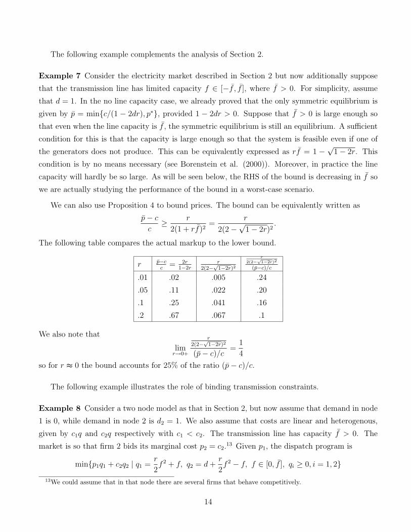
The following example complements the analysis of Section 2.

Example 7 Consider the electricity market described in Section 2 but now additionally suppose

that the transmission line has limited capacity f ∈ [−f , f ], where f > 0. For simplicity, assume

that d = 1. In the no line capacity case, we already proved that the only symmetric equilibrium is

given by p = minc/(1 − 2dr), p∗, provided 1 − 2dr > 0. Suppose that f > 0 is large enough so

that even when the line capacity is f , the symmetric equilibrium is still an equilibrium. A sufficient

condition for this is that the capacity is large enough so that the system is feasible even if one of

the generators does not produce. This can be equivalently expressed as rf = 1 −√

1− 2r. This

condition is by no means necessary (see Borenstein et al. (2000)). Moreover, in practice the line

capacity will hardly be so large. As will be seen below, the RHS of the bound is decreasing in f so

we are actually studying the performance of the bound in a worst-case scenario.

We can also use Proposition 4 to bound prices. The bound can be equivalently written as

p− cc≥ r

2(1 + rf)2=

r

2(2−√

1− 2r)2.

The following table compares the actual markup to the lower bound.

r p−cc

= 2r1−2r

r2(2−

√1−2r)2

r2(2−

√1−2r)2

(p−c)/c

.01 .02 .005 .24

.05 .11 .022 .20

.1 .25 .041 .16

.2 .67 .067 .1

We also note that

limr→0+

r2(2−

√1−2r)2

(p− c)/c=

1

4

so for r ≈ 0 the bound accounts for 25% of the ratio (p− c)/c.

The following example illustrates the role of binding transmission constraints.

Example 8 Consider a two node model as that in Section 2, but now assume that demand in node

1 is 0, while demand in node 2 is d2 = 1. We also assume that costs are linear and heterogenous,

given by c1q and c2q respectively with c1 < c2. The transmission line has capacity f > 0. The

market is so that firm 2 bids its marginal cost p2 = c2.13 Given p1, the dispatch program is

minp1q1 + c2q2 | q1 =r

2f 2 + f, q2 = d+

r

2f 2 − f, f ∈ [0, f ], qi ≥ 0, i = 1, 2

13We could assume that in that node there are several firms that behave competitively.

14

In this game, firm 1 is efficient because c1 < c2; however firm 1 is strategic so aims to maximize

profits. We will analyze the pricing behavior of firm 1 when f is close to 0 so that the line is

congested.

The optimal flow takes the form

f(p1) = minf , 1

r

c2 − p1

c2 + p1

The line will be congested when the price p1 is small enough so that f(p1) = f . Define p1 as the

only solution to 1rc2−p1c2+p1

= f and note that given that f is small enough, p1 = c21−rf1+rf

< c2 is in

fact the optimal equilibrium price. Indeed, as shown in the Appendix, this will indeed be firm 1’s

optimal strategy provided

2c2(rf)3 ≤(c2

1− rf1 + f

− c1

)(1 + rf)2

Therefore, for all such rf ,p1 − c1

c1

=c2/c1 − 1− (c2/c1 + 1)rf

1 + rf.

Let M(rf) be the RHS of this equality.

Proposition 4 offers the following estimate

p1 − c1

c1

≥ rf1 + rf

2

2(1 + rf)2.

Let m(rf) be the RHS of this equality. We set c1 = 1 and compute m(rf)/M(rf) for different

values of rf and c2 > 1.

rf c2 2 3 5

.01 .005 .002 .001

.05 .028 .013 .006

.1 .068 .029 .014

.2 .229 .076 .032

When rf is close to 0 (say, rf = 0.01), firm 1 is facing a demand which is almost inelastic and

therefore the equilibrium is so that firm 1 “undercuts” firm 2 by setting a price slightly below c2.

The bound, on the other hand, uses an estimate of the demand slope which is not precise. The

bound therefore gets worse the more room firm 1 has to undercut firm 2 (the more different c2 and

c1 are).

15

4.4 Extensions

The working paper version of the present work contains a number of extensions worth mention-

ing. First, demand is allowed to be random and the demand probability distribution is common

knowledge. Second, firms are allowed to bid supply functions which must belong to an exogenously

determined set (for example, firms bid convex nondecreasing cost functions). Third, each generator

is paid its bid plus a capacity premium (that is, the nodal prices are the shadow values of electricity).

It can shown that to deal with the existence problem, none of our working assumptions is required.

The key to prove that result is to introduce a topology on the sets of supply functions that ensures

continuity of solutions and Lagrange multipliers for minimization problems. In this paper we have

preferred to simplify the model in order to emphasize the economic and methodological substance

of our contribution. Consult Escobar and Jofre (2008) for the more general results. In our view,

the present framework could be used not only to analyze other phenomena in power markets (for

example, collusion or contracts), but also to study a wider class of network markets.

We have assumed that each electricity plant bids independently of the others. Of course, in

practice each plant is owned by a company that controls several generating units and, in principle,

can manage these units to maximize the sum of profits. After careful inspection of our results, the

monopolistic competition analysis can be extended to that more general context without significant

difficulty.

In some markets, transmission constraints are taken into account only after the spot market is

cleared. In others, firms’ bids include startup costs as well as schedules of marginal costs. Those

extensions are difficult because a key component of our analysis has been to see the dispatch

process as a consumer theory problem; the consumer theory analogy breaks down, for example,

when transmission constraints are considered only after the spot market is cleared. Some of our

qualitative insights may apply; it would be interesting to study how our results would extend to

those more realistic situations.

It would be interesting to explore how robust the results are to alternative market designs. It

is possible, for example, to use alternative pricing rules. Even with alternative pricing rules, our

estimates of demand’s slopes still apply. So, provided those pricing rules are sufficiently “smooth”

as functions of the bids, we conjecture that our method of proof should go through and prices should

be inefficiently high.

For numerical purposes, one would like to find sufficient conditions guaranteeing pure strategy

existence for the game among generators. (We only show that a mixed strategy equilibrium exists.)

However, the optimization problem characterizing the pure strategy best-replies is hardly a concave

16

program. Consequently, techniques based on Kakutani’s theorem (as our approach) do not seem

suitable for approaching the pure strategy equilibrium existence problem. We are also considering

such a broad class of electricity networks that does not seem possible to state a general pure strategy

equilibrium existence theorem. Our game does not possess a supermodular structure either. The

question of pure strategy existence is an interesting and demanding research avenue.14

5 Concluding Remarks

This paper shows that network constraints matter. While the complexity of power transfers has been

fully taken into account in an arbitrarily large network, the economics of competition in electricity

networks is surprising simple. Indeed, it has been argued that the model can be interpreted as a

game among monopolistic competitors facing Hicksian demands. In particular, the physics of power

flows renders the market naturally imperfectly competitive. Moreover, each generator exploits its

monopolistic position by setting prices strictly above marginal costs. The bound for market prices

show that the impact of any other network constraint can be measured by its effect on quantities

adjusted by a slope term.

Our model ignores and simplifies several aspects of actual markets, of course. We, however, hope

that the conceptualizations and insights offered by this work are deemed as useful by economists

who evaluate and design actual markets.

6 Appendix

This Appendix consists of three parts. In the first one, we go over the details of our leading example.

In the second one, we detail the calculations for the equilibrium in Example 8. Finally, we provide

proofs of the main results.

6.1 The Example

The ISO solves the following optimization problem

minp1q1 + p2q2 | q1 + f = d+r

2f 2, q2 − f = d+

r

2f 2, qi ≥ 0, i = 1, 2

14Hu and Ralph (2007) offer some results and examples.

17

Substituting for qi from the balance constraints and relaxing the constraints qi ≥ 0, we obtain

minp1(r

2f 2 − f) + p2(

r

2f 2 + f) | f ∈ R.

The only solution to this problem is given by

f(p1, p2) =1

r

p1 − p2

p1 + p2

.

Therefore, the optimal quantities are given by

Q1(p) = max0, d+r

2f(p)2 − f(p), Q2(p) = max0, d+

r

2f(p)2 + f(p).

Given p2 ≥ c, there exists p1 > p2 such that for all p1 < p1, Q1(p1, p2) > 0. On this set,

∂Q1(p1, p2)

∂p1

=1

r

(p2 − p1

p2 + p1

+ 1) −2p1

(p1 + p2)2= −1

r

4p21

(p1 + p2)3.

Now, define firm 1’s profit function as u1(p1, p2) = (p1 − c)Q1(p1, p2) and note that it is enough

to find firm 1’s best reply on the set [c, p1]. Let us look for a symmetric equilibrium p1 = p2 = p.

The necessary condition for an interior equilibrium p < p∗, ∂u1(p, p)/∂p1 = 0, has as only solution

p = c/(1 − 2rd). If c/(1 − 2dr) > p∗, then no interior equilibrium exists and the only solution to

the (symmetric) optimality conditions is p = p∗. To show that we indeed found an equilibrium, it

is enough to show that u1(p1, p2) is concave in p1 ∈ [c, p1] when p2 = p. But note that

∂2u1(p1, p2)

∂p21

=2∂Q1(p1, p2)

∂p1

+ (p1 − c)∂2Q1(p1, p2)

∂p21

=− 2

r

4p21

(p1 + p2)3+ (p1 − c)

−4

r

2p1p2 − p21

(p1 + p2)4

=− 4

r

( 2p21

(p1 + p2)3+ (p1 − c)

2p1p2 − p21

(p1 + p2)4

)=− 4p1

r

(p21 + 4p1p2 − 2cp2 + cp1

(p1 + p2)4

)

This second derivative is negative provided p21 + 4p1p2 − 2cp2 + cp1 ≥ 0. Given that p1 ≥ c and the

polynomial is increasing when p1 > 0, this condition is equivalent to 2c + 2p2 ≥ 0. The following

result summarizes the discussion.

Proposition 9 Suppose that 1− 2dr > 0. The only symmetric equilibrium for the two-node model

introduced in Section 2 is given by p = min c1−2dr

, p∗.

18

6.2 Example 8

When the line capacity is not binding, the quantity at which 1 is dispatched is given by the expression

Q1(p1) =1

r

c2 − p1

c2 + p1

+1

2r

(c2 − p1

c2 + p1

)2

so that the marginal utility is given by the expression

d

dp1

(p1 − c1)Q1(p1)|p1=p1 = f(1 +rf

2)− (1 + rf)

(c2

1− rf1 + rf

− c1

) 1

rc2

(1 + rf)2

2(rf)2

Bounding the first term on the RHS by f(1 + rf) shows that this derivative is negative under the

condition in the main text. Therefore, at p1 = p1 firm 1 is in the decreasing portion of the profit

function and from concavity (which can be shown as we did in the previous subsection) it follows

that firm will indeed find p1 = p1 optimal.

6.3 Proofs of Subsection 4.1

Proof of Lemma 1. It is straightforward to show that the dispatch problem can be rewritten as

DP (p) minfK∈RK ,q∈RG

∑v∈G

pvqv

Tv(fKv) = qv, v ∈ G

0 ≤ qv ≤ qv, v ∈ G

fK ∈ PΩ,

where PΩ ⊆ RK is the set of vectors fK such that there exists f−K with (fK , f−K) ∈ F (properly

ordered). Consider the following flow problem

minfK∈PPΩ

∑v∈G

pvTv(fKv), (6.1)

where

PPΩ = fK ∈ PΩ | Tv(fKv ≤ qv, )

is a convex set. Since pv > 0, if (fK , q) is a solution of DP , then fK is a solution to 6.1, Tv(fKv) = qv,

v ∈ G, and the optimal values of both problems coincide. But re > 0 and pv > 0, so the flow problem

(6.1) is a strictly convex program . We deduce the existence of a unique fK solving (6.1) which

in turn implies the desired uniqueness result. The continuity of (Qv)v∈G on ]0, p∗]|G| follows as a

consequence of Berge’s maximum theorem.

19

Proof of Proposition 2. Restrict each generator v to bid on the set Av := [c′v(0), p∗], and

consider any selection q(p) ∈ Q(p), p ∈ [0, p∗]|G|. From (A3), (qv)v∈G is a continuous function on∏v∈GAv. Therefore, the existence of equilibrium distributions (Fv)v∈G follows as a consequence of

Glicksberg’s theorem (see Fudenberg and Tirole (1991)).

Proofs of Subsection 4.2.

Consider the following abstract optimization problem

minx∈X

h(x), (6.2)

where X ⊆ RN and h : RN → R ∪ −∞,+∞, and we define A(h) ⊂ X as its set of optimal

solutions. We already argued that A is typically not differentiable. Under the second order growth

condition, however, A is a Lipschitz correspondence. For the sake of simplicity, we assume that A

is a function; see Bonnans and Shapiro (2000) for more general results.

We say that the abstract optimization problem (6.2) satisfies the second order growth condition

if there exists a neighborhood N of A(h) and σ > 0 such that

h(x) ≥ h(A(h)) + σ|x− A(h)|2, ∀x ∈ X ∩ V.

Lemma 10 Suppose that the abstract optimization problem (6.2) satisfies the second order growth

condition and h− h is a Lipschitz function with constant κ on X ∩N . Then

|A(h)− A(h)| ≤ κ

σ.

Proof. As h satisfies the second order growth condition,

σ|A(h)− A(h)|2 ≤ h(A(h))− h(A(h))

≤(h− h

)(A(h))−

(h− h

)(A(h))

≤ κ|A(h)− A(h)|,

where the last inequality follows since h− h is a Lipschitz function.

We now return to the analysis of solutions to the dispatch program. We define f(p) ∈ RK as

the solution to the flow problem (6.1). From the proof of Lemma 1, Qv(p) = Tv(fKv(p)). To prove

Proposition 3, we need the following second order growth condition.

20

Lemma 11 Suppose that pv > 0 for all v ∈ G. Then,∑v∈G

pvTv(f∗Kv

) ≥ OPT (p) + σ|f ∗K − f(p)|2

holds for all f ∗K ∈ PPΩ, where σ = 12

minv∈Gpv(mine∈Kv re).

Proof. Without loss of generality, suppose that OPT (p) = 0. It is not difficult to deduce that

Tv is strongly convex on RKv : For all γ ∈]0, 1[ and fKv , f∗Kv∈ RKv

Tv(γfKv + (1− γ)f ∗Kv) +

∑e∈Kv

re2γ(1− γ)|fe − f ∗e |2 ≤ γTv(fKv) + (1− γ)Tv(f

∗Kv

). (6.3)

Since pv > 0

pv

(Tv(γfKv + (1− γ)f ∗Kv

) +∑e∈Kv

re2γ(1− γ)|fe − f ∗e |2

)≤pv(γTv(fKv) + (1− γ)Tv(f

∗Kv

))

=γpvTv(fKv) + (1− γ)pvTv(f∗Kv

).

Now, pick fK , f∗K ∈ PPΩ and γ ∈]0, 1[. Since σ ≤ re

2pv,

pvTv(γfKv+(1− γ)f ∗Kv) + σ

∑e∈Kv

γ(1− γ)|fe − f ∗e |2 ≤

γpvTv(fKv) + (1− γ)pvTv(f∗Kv

).

By summing over v ∈ G, we deduce that∑v∈G

pvTv(γfKv+(1− γ)f ∗Kv) + σγ(1− γ)|fK − f ∗K |2

≤ γ∑v∈G

pvTv(fKv) + (1− γ)∑v∈G

pvTv(f∗Kv

).

Finally, since OPT (p) = 0,

0 ≤∑v∈G

pvTv(γfKv + (1− γ)f ∗Kv)

and then

σγ(1− γ)|f(p)− f ∗K |2 ≤ (1− γ)∑v∈G

pvTv(f∗Kv

)

for all f ∗K ∈ PPΩ. Since 1−γ > 0, σγ|f(p)−f ∗K |2 ≤∑

v∈G pvTv(f∗Kv

). By taking γ → 1 the claimed

inequality follows.

21

Proof of Proposition 3. For simplicity, suppose that fe ≥ |f e| for all e. Define p = (pw, p−w),

h(fK) =∑

v∈G pv(Tv(fKv)), and h(fK) = pw(Tw(fKw))+∑

v∈G\w pv(Tv(fKv)). As h(fK)− h(fK) =

pwTw(fKw)− pwTw(fKw),

|(h(fK)− h(fK))−(h(f ∗K)− h(f ∗K))|

≤ |pw − pw||Tw(fKw)− Tw(f ∗Kw)|

≤ |pw − pw||Kw|(1 + maxe∈Kw

ref e)|fK − f ∗K |.

By virtue of Lemmas 10 and 11,

|fKw(p)− fKw(p)| ≤ |fK(p)− fK(p)| ≤ |pw − pw||Kw|(1 + maxe∈Kw ref e)

σ

Consequently,

|Qw(p)−Qw(p)| ≤ |pw − pw|(|Kw|(1 + maxe∈Kw ref e)

)2

σ

which proves the result.

Proof of Proposition 4. Let pw < p∗ and let us prove 4.1. For each ∆p > 0 small enough

(such that pw + ∆p < p∗), α(pw) ≥ α(pw + ∆p). Consequently,

pwEp−w [Q(pw, p−w)]− Ep−w [cw(Qw(pw, p−w))] ≥

(pw + ∆p)Ep−w [Qw(pw + ∆p, p−w)]− Ep−w [cw(Qw(pw + ∆p, p−w))].

By reordering,

pwEp−w [Qw(pw, p−w)−Qw(pw + ∆p, p−w)] ≥ ∆pEp−w [Qw(pw + ∆p, p−w)]+

Ep−w [cw(Qw(pw, p−w))− cw(Qw(pw + ∆p, p−w))]. (6.4)

Take now a sequence of positive reals (∆pn)n∈N converging to 0 and a define L∆pn(p−w, d) =

c′w(Qw(pw + ∆pn, p−w)). Then,

L∆pn(p)(Qw(pw, p−w)−Qw(pw + ∆pn, p−w)

)≤ cw(Qw(pw, p−w))− cw(Qw(pw + ∆pn, p−w)).

Together with (6.4) this implies that

Ep−w [(pw − L∆pn(p)

)Qw(pw, p−w)−Qw(pw + ∆pn, p−w)

∆pn] ≥

Ep−w [Qw(pw + ∆pn, p−w)]

22

From Proposition 3

Ep−w [|pw − L∆pn(p)| ηw ] ≥ Ep−w [Qw(pw + ∆pn, p−w))]. (6.5)

Since (L∆pn)n∈N is a sequence of bounded functions, without loss of generality, it pointwise converges

to L. Since c′w is continuous, by taking n → +∞, we deduce that L(p) = c′w(Qw(pw, p−w)). By

virtue of (6.5), (4.1) follows from the Dominated Convergence Theorem.

Proof of Corollary 5. From Proposition 4, with probability 1, pw ≥ cw+ψw(pw). Thus for all q,

p·q ≥ c·q+ψ(p)·q. By taking min on both sides, it follows that OPT (p) ≥ OPT (c)+OPT (ψ(p)) ≥OPT (c) + κ(p). Clearly κ(p) is positive provided ψv(pv) > 0 for all v.

References

[1] Anderson S.., A. de Palma, and J.-F. Thisse (1989): “Spatial Price Policies Reconsidered,” The

Journal of Industrial Economics, 38, 1-18.

[2] Bonnans, J.F., and A. Shapiro (2000): Perturbation Analysis of Optimization Problems. Berlin,

Springer-Verlag.

[3] Borenstein, S., J. Bushnell, and S. Stoft (2000): “The Competitive Effects of Transmission

Capacity in A Deregulated Electricity Industry,” RAND Journal of Economics, 31, 294-325.

[4] Chao, H.-P., and S. Peck (1996): “A Market Mechanism for Electric Power Transmission,”

Journal of Regulatory Economics, 10, 25-59.

[5] Cho, I. (2003):“Competitive Equilibrium in a Radial Network,” Rand Journal of Economics,

34, 438-460.

[6] Day, C., B. Hobbs, and J.-S. Pang (2002): “Oligopolistic Competition in Power Markets: A

Conjectured Supply Function Approach”, IEEE Transactions on Power Systems, 17, 597-607.

[7] D’aspremont, C., J. Jaskold-Gabszewicz, and J.-F. Thisse (1979):“On Hotelling’s Stability in

Competition” Econometrica, 47, 1145-1150.

[8] A. Ehrenmann, and Neuhoff, K. (2004): “A Comparison of Electricity Market Designs in Net-

works,” Cambridge Working Papers in Economics 0341, Faculty of Economics, University of

Cambridge.

23

[9] Escobar, J.F., A. Jofre (2008): “Equilibrium Analysis of Electricity Auctions,” Working paper.

[10] von der Fehr, N.-H., and D. Harbord (1993): “Spot Market Competition in the UK Electricity

Industry,” Economic Journal, 103, 531-546.

[11] Fabra, N., N.-H. von der Fehr, and D. Harbord (2006):“Designing Electricty Auctions,” Rand

Journal of Economics, 37, 23-46.

[12] Fudenberg D., and J. Tirole (1991): Game Theory. Cambridge, MIT Press.

[13] Green, R.J., and D. Newbery (1992): “Competition in the British Electricity Spot Market,”

Journal of Political Economy, 100, 929-953.

[14] Green, R.J. (1999): “The Electricity Contract Market in England and Wales,” Journal of

Industrial Economics, 47, 107-124.

[15] Hobbs, B.F. (1986): “Mill Pricing Versus Spatial Price Discrimination Under Bertrand and

Cournot Spatial Competition,” The Journal of Industrial Economics, 35, 173-191.

[16] Hobbs, B.F., C.B. Metzler, and J.-S. Pang (2000): “Strategic Gaming Analysis for Electric

Power Networks: An MPEC Approach,” IEEE Transactions on Power Systems, 15 , 638-645.

[17] Hotelling, H. (1929): “Stability in Competition”, Economic Journal, 39, 41-57.

[18] Hu, W., and D. Ralph (2007): “Using EPECs To Model Bilevel Games in Restructured Elec-

tricity Markets with Locational Prices,” Operations Research, 55, 809-827.

[19] Joskow, P., and J. Tirole (2000):“Transmission Rights and Market Power on Electric Power

Networks,” Rand Journal of Economics, 31, 450-487.

[20] Klemperer P., and M. Meyer (1989): “Supply Function Equilibria in Oligopoly under Uncer-

tainty,” Econometrica, 57, 1243-1277.

[21] Milgrom P., and I. Segal (2002): “Envelope Theorems for Arbitrary Choice Sets,” Economet-

rica, 70, 583-601.

[22] Mulligan G.F., and T.J. Fik (1994): “Price and Location Conjectures in Medium- and Long-

Run Spatial Competition Models,” Journal of Regional Science, 34, 179 - 198.

[23] Newbery, David (1998): “Competition, Contracts, and Entry in the Electricity Spot Market,”

RAND Journal of Economics, 29, 726-749.

24

[24] Pang, J.-S., and B. Hobbs (2004): “Spatial Oligopolistic Equilibria with Arbitrage, Shared

Resources, and Price Functions Conjetures,” Mathematical Programming, Series B, 101, 57-94.

[25] Schweppe, F., M. Caramanis, R. Tabors, and R. Bohn (1988): Spot Pricing of Electricity.

Boston, Kluwer Academic Publishers.

[26] Vives, X. (1999): Oligopoly Pricing: Old Ideas and New Tools. Cambridge, MIT Press.

[27] Wei, J.-Y., and Y. Smeers (1999): “Spatial Oligopolistic Models with Cournot Firms and

Regulated Transmission Prices,” Operations Research, 47, 102-112.

[28] Wilson, R. (2002): “Architecture of Power Markets,” Econometrica, 70, 1299-1340.

25